Optimising a Tournament for Use with Ranking Algorithms

Clayton D’Souza

March 13, 2010

Abstract

The top division in American college football known as the Football Bowl Sub-

division uses a series of polls and computerised ranking systems to determine the

match-ups for the postseason bowl competition. In this dissertation, an algorithm

known as the Random Walker Ranking system (RWR) is considered. An alterna-

tive formulation in terms of Markov chains is provided and tournament schedules

that return the a priori ranking of the participants under the RWR algorithm are

investigated.

1 Introduction

One of the primary motivations of a sports tournament is to determine the best com-

petitor. In different sports, various formats are used with their own advantages and

disadvantages.

Many sports opt for a round-robin tournament in which every competitor plays

against every other competitor a fixed number of times. Typically, this is once or twice

and is referred to as a single round-robin or double round-robin, respectively. An ex-

ample of a double round-robin is the format used in the top division of the professional

association football league in England known as the Barclays Premier League [11]. Each

team plays each other twice; one match at each team’s home ground. Wins are awarded

three points and draws are awarded one point. At the end of the season, the team with

the most number of points is the winner. One advantage of a round-robin1 tournament is

that each team has a schedule of the same strength. However, it requires a large number

of games, which is usually not feasible. If there are n teams, a robin-robin would require(n2

)games.

1A round-robin tournament henceforth refers to a single round-robin tournament unless stated oth-erwise.

1

Other sports such as tennis [16] and track athletics [14] use knock out or elimination

tournaments. These are structured into rounds in which the stronger competitors, as

determined by the outcome of a match/race proceed to the next round. With each suc-

cessive round, the number of competitors decreases until the final round which consists

of just two players. The winner of this match is declared as the champion. Single elim-

ination tournaments are most common in which only the winner proceeds to the next

round but variants exist where some of losing competitors can also progress. A knock

out tournament is efficient as it determines the winner with fewest games played. How-

ever, a drawback is most teams are eliminated after playing a small number of games

and thus a single poor performance or unlucky result can lead to elimination.

As well as determining the single strongest competitor, a tournament can also be

used to produce seedings for future competitions by providing an aggregate ranking of

the teams/players. This is particularly common in American sports such as professional

baseball, football and basketball as well as college basketball and baseball where the

champion is determined through a post season competition or playoff for the participants.

The prime motivating example is the top division of NCAA American College Foot-

ball known as the Football Bowl Subdivision (FBS). This consists of approximately 120

college teams who are organised into smaller conferences of around ten teams each. Typ-

ically, each team typically plays some teams within its own conference and plays some

teams from other conferences. These games make up the regular season, which is used

to determine the match-ups in the post season competition, known as the bowl season.

The FBS does not have a playoff system to determine its champion. Instead an inde-

pendent body, the Bowl Championship Series (BCS) committee aggregates a series of

expert poll results and computer ranking systems to determine the top ten teams [2].

The two “best” teams are invited to play in the BCS National Championship game, with

the winner declared champion. The eight other teams compete in other prestigious bowl

games but cannot win the championship that year.

The purpose of this dissertation is to investigate the structure of tournaments for use

with a computer ranking system. The BCS selection process includes such ranking algo-

rithms as part of its framework. Although some of the algorithms have been disclosed,

the workings of others remain secret. This, combined with the difficulty of understand-

ing for the lay sports fan has led to distrust in the ranking process whenever faced with

perverse results. Hence, it is desirable that the ranking system used with a tournament

be intuitive yet also provide results that agree with established sports knowledge. Such

a system is discussed in section 2.

In order to optimise a tournament, we will need to establish what is meant by a good

2

tournament. This is done in section 3. We consider a ranking as a permutation of the

teams and develop a metric that allows the comparison of rankings, including ones with

ties.

In section 4, we examine two different tournament structures and investigate their

properties analytically and using two computer heuristics. We find that both tournament

structures are strong in some aspects but deficient in others. A computer algorithm for

generating permutations is also considered.

In section 5, we develop a method to combine the desirable properties of both tour-

naments considered in section 4. The results for tournaments with 20, 40 and 120 teams

are reported.

Finally, in section 6, we review the dissertation and provide a conclusion.

2 Random Walker Ranking System

2.1 Background

We consider the random walker model devised by Callaghan, Mucha and Porter (CMP)

[3]. This ranks the football teams in the NCAA FBS by setting up a graph with the

vertices corresponding to the teams and edges representing matches between teams. A

random walker now traverses this network; when at a vertex, it picks a match played by

the team uniformly at random and moves to the winner with probability p ∈ (0.5, 1).

This interval for p ensures that the walker will favour winning teams but allows for the

possibility that the better team lost.2 The rate at which the walker considers a game is

independent of the total games played by a team. This ensures there is no advantage by

playing more games.

The random walker can be thought of as an idealised voter deciding on the strongest

team. The voter believes the winner is the better team, a fraction p of the time. Hence

the voter uses the intuition most fans use to rank teams,“My team is better than yours

because my team defeated yours”, allowing for the possibility of an unlucky defeat. It

changes its preferred team, by selecting a opponent of its current preference and going

with the winner of the match with probability p. Some occasions, the voter may decide

to stick with its current preference. Given enough time, this voter will consider every

match between every team. However, it will never decide on a strongest team, i.e. a

single random walker will traverse the network forever.

Thus CMP consider a constant population of random walkers. Provided the network

2More detail is given in section

3

is connected, the population of walkers will converge to a unique equilibrium distribution.

By counting the number of random walkers gathered on a vertex, CMP obtain a ranking

for the teams, as better teams will have accumulated more random walkers.

To set up the problem mathematically, suppose there are n teams. Let wi be the

number of wins by team i and let li be the number of losses. Let Sij be the number of

games played between teams i and j and let Aij be the number of times i beat j minus

the number of times j beat i. For example, if team 1 played team 2 three times with team

1 winning one match and team 2 winning two matches, then S12 = S21 = 3, A12 = −1

and A21 = 1. Let v be a vector of length n with each entry containing the expected

population of random walkers at a given vertex, i.e. the expected number of votes for

a team. The total number of votes is constant and without loss of generality can be

normalised to 1 i.e∑vi = T = 1 . The random walk is quantified by the homogeneous

ordinary differential (ODE) equation v′ = Dv.

Equation 2.1. The matrix D is for i, j ∈ {1, ..., n} :

Dii = −pli − (1− p)wi (1)

Dij =Sij2

+2p− 1

2Aij for i 6= j

The limiting distributions are the fixed points of this set of differential equations.

These can be obtained by solving the equation:

Dv = 0. (2)

Hence v is a vector in the kernel of D. Provided the network of teams consists of a single

connected component and p ∈ (0.5, 1), v is unique by the Perron-Frobenius theorem, as

described by [9]. In fact, we always have a single connected component by week 3, due

to the early season games generally being between teams in different divisions [3].

2.2 Formulation with Markov Chains

In this section, we will consider one voter making a decision on its choice of strongest

team. The random walk undertaken by the voter can be expressed in the form of a

Markov chain. There are two alternative formulations depending on if the time taken

for voters to reach equilibrium is discrete or continuous. We start by describing the

continuous time process using definitions from [6].

Let X = {X(t) : t ≥ 0} be a family of random variables taking values in some finite

4

state space R, with time indexed by the half line [0,∞). The process X is a continuous

time Markov chain if satisfies the following condition:

Definition 2.2. The process X satisfies the Markov property if:

P(X(tn) = j|X(ti) = ii, . . . , X(tn−1) = in−1) = P(X(tn) = j|X(tn−1) = in−1) (3)

for all j, i1, . . . , in−1 ∈ R and any sequence t1 < t2 < ... < tn of times.

In this case, X(t) represents the voter’s choice of strongest team at time t and R is

set of all teams that play in the FBS plus a hypothetical team “non FBS Team” that

represents any team outside the FBS. Teams within the FBS occasionally play teams

outside the division and it is convenient to represent all of these teams as one. This

approximation was found to be reasonable as most non FBS teams are much weaker

than FBS teams and so will not affect the rankings of the FBS teams much apart from

penalising those teams which they defeat [3].

In order to explain the evolution of X, we will need some basic definitions [6].

Definition 2.3. The transition probability pij(s, t) is defined to be:

pij(s, t) = P(X(t) = j |X(s) = i) for s ≤ t (4)

Definition 2.4. A Markov chain is called homogeneous if pij(s, t) = pij(0, t− s) for all

i, j, s, t

We assume X is a homogeneous chain, and write Pt for the |R| × |R| matrix with

entries pij(t).

Definition 2.5. The generator matrix Q is defined to be:

Q = limh↓0

1

h(Ph − I) (5)

We express the random walk as a continuous time Markov chain (CTMC) by speci-

fying Q. We use a number of definitions, as made by Young [19]:

5

Definition 2.6.

Let W be a matrix such that Wij is the number of times team i beat team j.

Let L be a matrix such that Lij is the number of times team i lost to team j.

Let S = W + L so Sij = Sji is the number of games played by team i against team j.

Let wi =∑

jWij be the number of wins for team i

Let li =∑

j Lij be the number of losses for team i

The matrix S provides the schedule of the tournament i.e. a description of all the

matches within the tournament.

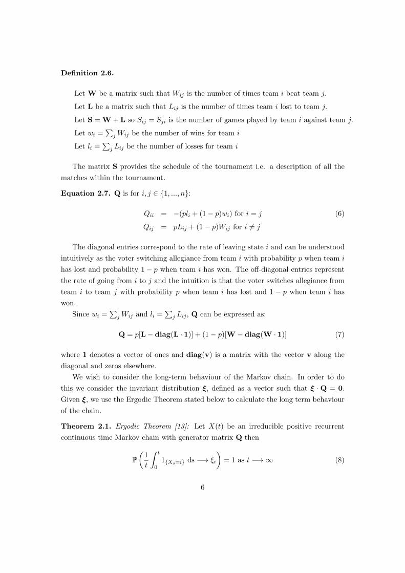
Equation 2.7. Q is for i, j ∈ {1, ..., n}:

Qii = −(pli + (1− p)wi) for i = j (6)

Qij = pLij + (1− p)Wij for i 6= j

The diagonal entries correspond to the rate of leaving state i and can be understood

intuitively as the voter switching allegiance from team i with probability p when team i

has lost and probability 1− p when team i has won. The off-diagonal entries represent

the rate of going from i to j and the intuition is that the voter switches allegiance from

team i to team j with probability p when team i has lost and 1 − p when team i has

won.

Since wi =∑

jWij and li =∑

j Lij , Q can be expressed as:

Q = p[L− diag(L · 1)] + (1− p)[W − diag(W · 1)] (7)

where 1 denotes a vector of ones and diag(v) is a matrix with the vector v along the

diagonal and zeros elsewhere.

We wish to consider the long-term behaviour of the Markov chain. In order to do

this we consider the invariant distribution ξ, defined as a vector such that ξ · Q = 0.

Given ξ, we use the Ergodic Theorem stated below to calculate the long term behaviour

of the chain.

Theorem 2.1. Ergodic Theorem [13]: Let X(t) be an irreducible positive recurrent

continuous time Markov chain with generator matrix Q then

P(

1

t

∫ t

01{Xs=i} ds −→ ξi

)= 1 as t −→∞ (8)

6

Provided p < 1 and the graph contains a single connected component, the assump-

tions of (8) are satisfied. From Norris [13], a state i is positive recurrent if

P(t ≥ 0 : Xt = i is unbounded |X0 = i) = 1. A Markov chain is recurrent if its jump

chain is recurrent, which in this case it is as it is a finite closed class.

This gives another interpretation of the voter. The stationary distribution gives the

long term average the voter spends in each state i.e. what proportion of time the voter

decides that team is the best. Seeing as the voter prefers stronger teams, we obtain a

ranking by taking an ordering of ξ. We compare this ranking to the ranking obtained

from the ODE formulation.

Proposition 2.2. The rankings from the continuous time Markov chain approach and

the ordinary differential equation approach are the same.

Proof. The diagonal entries of the rate matrix D and the generator Q are the same. In

fact, D = QT because for i 6= j:

Dij =Sij2

+2p− 1

2Aij (9)

=1

2(Wij + Lij) +

2p− 1

2(Wij − Lij)

=1 + 2p− 1

2Wij +

1− 2p+ 1

2Lij

= pWij + (1− p)Lij= pLji + (1− p)Wji

= Qji

To find the stationary distribution ξ of the CTMC, one solves ξ · Q = (0, . . . , 0). By

taking transposes, this is equivalent to the equation solved by CMP: D · v = 0 where

v = ξT . Hence the ranking obtained from both approaches is identical.

An alternative way to describe the random walker model is through a discrete time

Markov chain (DTMC). The process X(t) still takes values from R but is now time

is indexed by the non-negative integers. The transition matrix for the DTMC can be

derived from the generator of the CTMC, Q:

7

0 = ξ ·Q (10)

0 = ξ ·Q + ξ − ξ

ξ = ξ ·Q + ξ · I

ξ = ξ · (Q + I)

Thus we see P = Q + I is the transition matrix with ξ as its stationary distribution

as the row sums of P are 1. In the discrete case, the population interpretation considered

in the ODE formulation is preferred. Rather than each walker considering each game

at a given rate, one game is picked at random from the whole schedule, and the walkers

involved undertake the appropriate probabilistic actions. There is no advantage given

to teams that play more games than other teams. We deduce this by observing the

probability of the chain jumping from a state i to itself, Pii = 1 − [pli + (1 − p)wi]

decreases as the number of games played increases. As this Markov chain is completely

determined by Q, we will also obtain the same ranking using this model.

In this section, a one parameter model was outlined. It is natural to ask the question,

“What is an appropriate value of p?” The parameter p gives the probability that the

walker jumps from vertex i to j given that team i beat team j. This implies that p can

be interpreted as the probability that team i is better than team j given i beat j. From

[3], a value of around 0.75 is found to be give good empirical results. The rationale for

this is that values close to 1 over-emphasize unbeaten sequences, neglecting the quality

of opponent whereas values close to 0.5 attach too much weight to the difficulty of a

team’s fixture list. In this sense, 0.75 provides a happy medium.

3 Comparing Rankings

To be able to optimise a tournament, we will need to define the concept of a good

tournament. T. McGarry and R. W. Schutz (MS) [12] suggest the best tournament is

the structure that best ranks the players according to their a priori standings 3. MS

define head-to-head win probabilities for eight teams. Through running simulations with

various tournament structure, MS determine the difference between the observed rank

of the teams and the expected rank. However, in the case of NCAA FBS, there are 120

teams so this approach is impractical. Hence a simplifying assumption is required: To

3Other suggestions include:

8

model the head-to-head win probabilities we use the sure win probability model as used

by [10]. Initially, we provide a definition for a ranking.

Definition 3.1. Let [n] = {1, . . . , n} be a set of teams for n ∈ N. A ranking of the

teams is a permutation of [n]. Team i is given rank ri. We consider the strongest team

to be given rank 1 and the weakest team rank n.

Definition 3.2. Sure Win Probability: Suppose we have team i (resp. j) with ranking

ri (resp. rj). Then

P(Team i defeats team j) =

{1 if ri < rj

0 if ri > rj(11)

Suppose we have a hypothetical tournament schedule S, as in definition 2.6, the sure

win probability allows us to simulate W as in 2.6 and then Q defined in 6. The ranking

arising under S can then be calculated by working out the ordering of the stationary

distribution. This can be done for arbitrary S to give a unique ranking provided the

conditions of theorem 2.1 are satisfied.

We wish to consider how different are two rankings arising from this method. A well

known metric on set of permutations is known as Spearman’s Footrule [4].

Definition 3.3. Let Πn be the set of permutations of length n. Let σ, π ∈ Πn. Spear-

man’s Footrule, D is defined as:

D(π, σ) =n∑i=1

|σ(i)− π(i)| (12)

However, the random walker ranking procedure can produce ties and not give a

proper permutation. We introduce some terminology [5]:

Definition 3.4. A Bucket order is a transitive binary relation ≺ on a domain X for

which there are sets B1, ...,Bt (the buckets) that form a partition of the domain such

that x ≺ y if and only if there exist i, j with i < j such that x ∈ Bi and y ∈ Bj . If

x ≺ y, we say x precedes y. The elements of a bucket are considered to be tied. In a

permutation, every bucket is of size 1

Definition 3.5. The position of a bucket Bj , defined as pos(Bj) = (∑

i<j |Bi|) +1+|Bj |

2

can be thought of as the average location in the bucket.

9

A ranking with ties is known as a partial ranking. We associate a partial ranking σ

to a bucket ordering by letting σ(x) = pos(B) where x ∈ B. Spearman’s footrule now

generalises to partial rankings as required.

4 Properties of Specific Tournaments

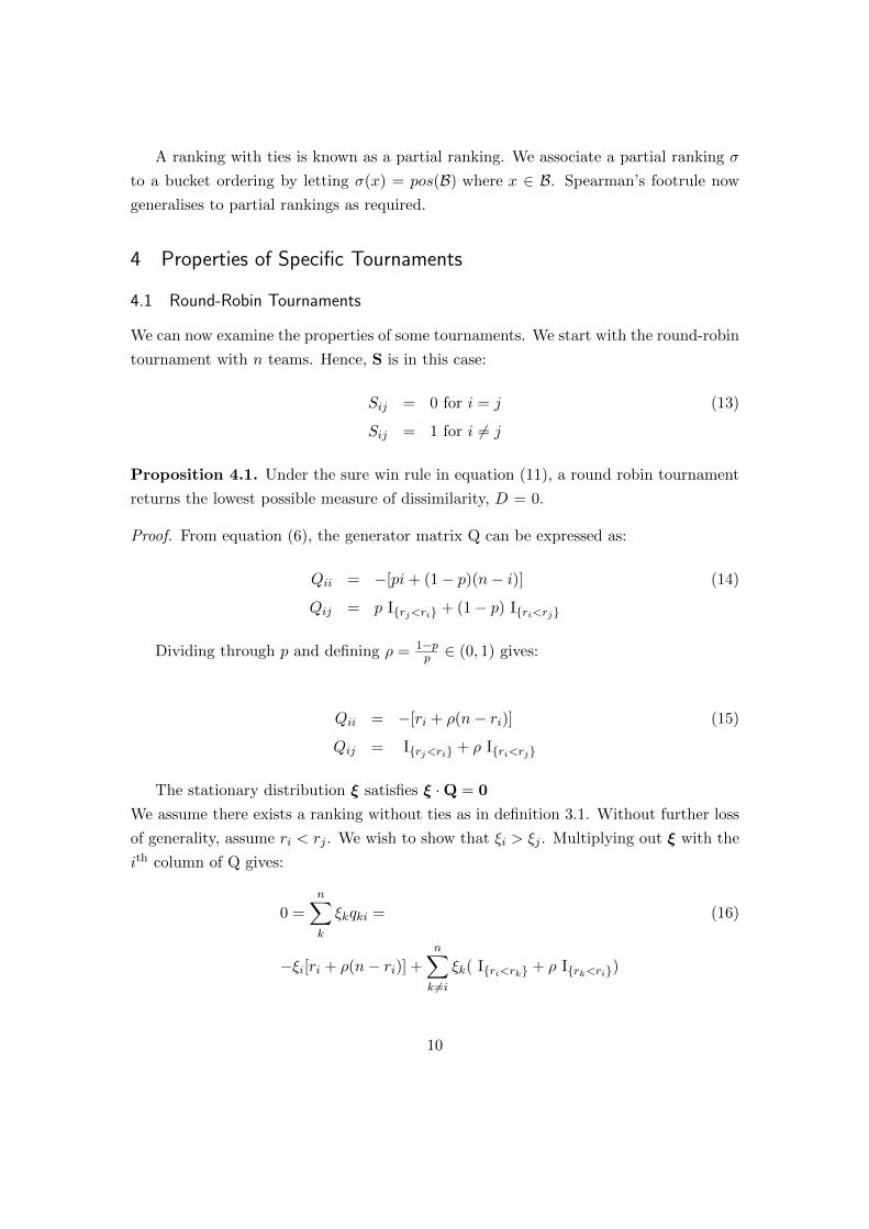
4.1 Round-Robin Tournaments

We can now examine the properties of some tournaments. We start with the round-robin

tournament with n teams. Hence, S is in this case:

Sij = 0 for i = j (13)

Sij = 1 for i 6= j

Proposition 4.1. Under the sure win rule in equation (11), a round robin tournament

returns the lowest possible measure of dissimilarity, D = 0.

Proof. From equation (6), the generator matrix Q can be expressed as:

Qii = −[pi+ (1− p)(n− i)] (14)

Qij = p I{rj<ri} + (1− p) I{ri<rj}

Dividing through p and defining ρ = 1−pp ∈ (0, 1) gives:

Qii = −[ri + ρ(n− ri)] (15)

Qij = I{rj<ri} + ρ I{ri<rj}

The stationary distribution ξ satisfies ξ ·Q = 0

We assume there exists a ranking without ties as in definition 3.1. Without further loss

of generality, assume ri < rj . We wish to show that ξi > ξj . Multiplying out ξ with the

ith column of Q gives:

0 =n∑k

ξkqki = (16)

−ξi[ri + ρ(n− ri)] +n∑k 6=i

ξk( I{ri<rk} + ρ I{rk<ri})

10

Similarly, the jth column of Q gives:

0 =n∑k

ξkqki = (17)

−ξj [rj + ρ(n− rj)] +n∑k 6=j

ξk( I{rj<rk} + ρ I{rk<rj})

Subtracting (17) from (16) gives:

0 = [rjξj − riξi] + ρ[n(ξj − ξi) + riξi − rjξj ] + ξj − ρξi + (18)n∑

k 6=i,jξk[ I{ri<rk} − I{rj<rk}] + ρξk[ I{rk<ri} − I{rk<rj}]

Note that the only contribution from the summation comes from the case when

ri < rk < rj . In all other cases of ri, rk, rj the indicator functions cancel. The possibility

of I{rj<rk} = 1 and I{rk<ri} = 1 cannot occur as it implies rj < rk < ri but by

assumption ri < rj . Hence (18) becomes:

0 = rjξj − riξi + ρ[n(ξj − ξi) + riξi − rjξj ] + ξj − ρξi + (19)n∑

{k: ri<rk<rj}

ξk − ρξk

The term within the summation, (1− ρ)ξk , is positive because ρ ∈ (0, 1). Hence,

0 > rjξj − riξi + ρ[n(ξj − ξi) + riξi − rjξj ] + ξj − ρξi (20)

= rjξj − riξi + ρ(riξi − rjξj) + ρn(ξj − ξi) + ξj − ρξi= (1− ρ)(rjξj − riξi) + ρn(ξj − ξi) + ξj − ρξi= (1− ρ)(rjξj − rjξi + rjξi − riξi) + ρn(ξj − ξi) + ξj − ρξj + ρξj − ρξi= (1− ρ)[rj(ξj − ξi) + ξi(rj − ri)︸ ︷︷ ︸

>0

] + ρn(ξj − ξi) + (1− ρ)ξj︸ ︷︷ ︸>0

+ρ(ξj − ξi)

> (ξj − ξi)[(1− ρ)rj + ρn+ ρ︸ ︷︷ ︸>0

].

Hence ξj−ξi < 0, so team i is ranked above j. Because i and j were arbitrary, the whole

ranking is recovered. The random walker ranking is the same as the original ranking,

thus D = 0 as required.

11

4.2 Permutations

Another advantage of the round robin tournament is that it is unaffected by the permu-

tations of the initial ranking or seeding of the teams. This is because every team has the

same fixtures so there is no advantage by being seeded higher. However, this is not the

case with tournaments without this symmetry. In order to address this, we permute the

initial ranking of the teams and measure how well the random walker ranking recovers

this permutation. Let σ be a random permutation of n teams. This is the initial seeding

of the teams such that ri = σ(i). Using σ and S, we calculate W and consequently

Q. We can then calculate the random walker (partial) ranking, π and work out D as

in equation (12). Ideally, we would like to consider every permutation of the teams.

However the number of permutations for n teams is n!, so it soon becomes too large for

this to be be practical. Hence we use Monte Carlo methods. We generate a fixed number

of random permutations from the n! possibilities, noting the value of D we obtain for

each permutation. We then take the mean value of Ds obtained. This gives an overall

indication of the predictive power of the tournament, mean D (denoted as D). The

accuracy of D increases as the number of permutations considered increases.

We utilise the algorithm to generate permutations known as the Random Permu-

tation Generator [15]. Let Πn be the set of permutations on n objects denoted as

[n] = {1, . . . , n}. The algorithm draws elements π1, π2, . . . , πn from [n] without replace-

ment and combines them sequentially to form π1π2 . . . πn = π ∈ Πn. We specify the

distribution of permutations through the parameter θ ∈ [0, 1]. (This choice of parame-

terisation is explained on page 13).

Definition 4.1. Using θ, we define a a n× 1 control vector z such that.

zi = θ · zi−1, i = 2, . . . , n (21)∑j

zj = 1 (22)

The ith entry of this control vector zi gives the probability that the element i is the

first entry i.e. π1 = i. After the first entry is drawn, we define a new control vector,

where the probability of drawing the element that we have just drawn is set to zero, and

the remaining probabilities are normalised so that they sum to one. The second entry,

π2 is drawn from this distribution. Again, we define a new vector, setting the probability

of all elements that have been drawn to zero and normalising the probability of those

elements that have not been yet drawn so that their sum is one. This continues until all

elements have been drawn, giving a permutation of [n].

12

Formally, suppose R ⊆ [n] represents the elements that have already been drawn.

Definition 4.2. The control vector given R denoted z|R is for all i ∈ [n]

z′i =

0 if i ∈ R

zi∑i/∈R zi

if i /∈ R(23)

Initially, set R = ∅, noting that z|∅ = z. For each step, we draw πi from the

distribution specified by z|R and then add the element πi we have just drawn to R.

This terminates when |R| = n so all elements have been drawn. The string given by

π1 . . . πn gives a permutation.

There are three cases for θ: θ = 0, θ ∈ (0, 1) and θ = 1. If we set θ = 1, according to

definition 4.1 the control vector z becomes [ 1n , . . . ,1n ]T . The first element, π1 is chosen

uniformly from [n]. After |R| elements have been drawn, it is clear that all non-zero

elements of z′ are 1n−|R| , and so are equally likely. This means that all n! permutations

are equally likely so we draw a permutation uniformly from Πn.

We assert the following property of the random permutation generator (see [15] for

proof).

Proposition 4.2. Let i,j ∈ [n]. The probability that i precedes j in any permutation

generated is given by:

P(i precedes j) =zi

zi + zj(24)

Consider θ → 0. The probability, P(i precedes i+ 1) = zizi+zi+1

= zizi+θzi

→ 1. Hence,

as θ → 0, the permutation 12 . . . n will generated almost surely.

Hence, θ provides a convenient index for how uniform the distribution of permuta-

tions returned by the generator is. When θ = 1, it is the uniform over all n! possibilities

whereas if θ = 0, all the probability mass is assigned to one permutation. In the open

interval (0, 1), a higher value of θ implies a more even spread of probability amongst the

n elements. Throughout the rest of this dissertation, we assume θ = 1.

4.3 Tournaments with Minimal Games

Round-robin tournaments have good properties with regards to the lowest D and symme-

try but they have the largest number of games. We now look at tournaments with small

number of games. The random walker algorithm requires a single connected component

of the graph of teams for a unique stationary distribution. The graph of a tournament

which achieves this with the fewest possible games (i.e edges) corresponds to a tree, a

13

graph with no cycles. A tree on n vertices has n − 1 edges [1], so this is the minimum

number of games that can be played.

We now search for the worst possible case in terms of D. It is unknown what the

highest possible D would be for a tournament with n teams and n − 1 games. Hence

we calculate it empirically. There are a number of heuristics that can be used for this

purpose. The solution we obtain from heuristic is not expected to be the optimal solution

but it provides a good solution in reasonable time.

The simplest heuristic is the Greedy Algorithm: Suppose n is fixed. We start with

a connected schedule S with n − 1 games. At each step, we perturb S by deleting

a random game and adding a random game to give S′, ensuring the network is still

connected. This can be guaranteed by noting that because S is a tree, deleting an edge

will always disconnected the graph into two components S1 and S2. We pick any vertex

uniformly in S1 and join it to a random vertex in S2 to create a tree on n vertices, S′ .

We calculate D of S′ through calculating a fixed number of permutations as described

above. If D of S′ is greater than D of S, we set S = S′ for the next step. Otherwise, we

try a new perturbation of S. We do this for a fixed number of trials, in this case 10000.

This algorithm is run for a number of different n values, with the results given in Table

2.

The greedy algorithm is simple to implement but is expected to get stuck at a

suboptimal local maximum as it will never move to a solution S′ with worse D. An

algorithm that attempts to rectify this is simulated annealing [17]. This algorithm

is named after a technique in metalworking, in which a material is heated and then

cooled in a controlled fashion to reduce its internal structure to the lowest energy state.

The heating causes the atoms of the material to move freely with respect to each other,

randomising their distribution; and the subsequent slow cooling gives the atoms a chance

to form a structure with lower energy than the initial state. Analogously, the algorithm

attempts to minimise a objective function E (analogue of energy). Given the current

solution, the algorithm proposes a new “nearby” solution and selects it proportional to

the difference of the energy states of the two solutions and a control variable T (analogue

of temperature). If the current solution has energy E1 and the proposed solution has

E2, the probability that the algorithm adopts E2 as its new current solution is:

pA = min{exp{E1 − E2

T}, 1} (25)

If E2 < E1, pA = 1, so the algorithm always selects a move that reduces E (a downhill

move). However, if the proposed solution has higher E, there is still a chance that it will

14

be accepted and hence the algorithm can escape local minima. The dependency on T

is such that when T is large, the algorithm has a high chance of accepting uphill moves

so explores a large proportion of the solution space but as T decreases the algorithm

increasingly prefers downhill moves. An annealing schedule is required that specifies

when and by how much to decrease T. Trial and error is required to set up the annealing

schedule as if T is reduced too quickly, the algorithm may not explore enough of the

solution space and get caught at a local minima but if T is reduced too slowly, the

computation will be inefficient and run longer than necessary.

In order to set up our problem to use simulated annealing, we provide the following

elements: S gives a description of a possible solution i.e. the adjacency matrix of a tree

on n vertices. The method of perturbing S to give S′ given in the Greedy Algorithm

allows the generation of new “nearby” solutions. Since we are seeking to maximise D,

an appropriate choice of E is −D which we seek to minimise. We generate an annealing

schedule through experimentation: By running a few hundred iterations of the genera-

tor, we can observe the difference in E at each step. Initially, we want pA to be high

so we explore the solution space adequately. Hence , we set T much larger than the

maximum difference, so even uphill moves have a good chance of being accepted (be-

cause E1−E2T will be close to 0, pA will be close to 1) . Rather than prescribing exactly

how and when T is reduced, we set clauses that force T to be reduced. For a given T ,

we generate a maximum of number of candidate solutions, K. We keep track of the

number of accepted solutions, J for a given temperature. The temperature is reduced

by a constant multiplicative factor α either when K solutions have been considered or

we hit a prescribed limit, L of accepted solutions i.e. J > L (meaning we have found a

promising subset of solution space). The algorithm terminates when we have considered

a specified number of temperatures, nmax, or for a given temperature, all K solutions

have been rejected. Following the example given by the simulated annealing algorithm

for the travelling salesman problem given in [17], we set the parameters as follows:

Parameter Value

Starting T 5

α 0.9

K 50n

L 10n

nmax 100

Table 1: Parameter values for simulated annealling

15

The results for the simulated annealing are also given in table 2.

n Greedy Algorithm Simulated Anneal

20 87.349 87.284

40 371.871 374.752

120 3227.843 3243.767

Table 2: D returned by the algorithms

Thus we have a answer for what is the worst D for a tree tournament; one with n−1

games. We have an idea of the magnitude of D because D is a empirical realisation of

D. Moreover, from conducting empirical trials, we believe these values give the worst

possible D for all connected tournaments with n teams. The minimum D is achieved

when the maximum number of games has been played i.e. in the case of a round-robin

tournament.

5 Developing Tournaments

In the previous section, two different tournaments were examined. It was shown that

round-robin tournament was optimal in D but had the largest number of games. Con-

versely, a tree tournament had the minimum number of games but the worst possible

D. Is possible to find a tournament which combines the good properties of these two

tournament types? i.e. A low D and a small number of games.

We require a rule to evaluate the fitness of a tournament.

Definition 5.1. Given a tournament S, the fitness of S is:

F (x, y) = βx− (n− 1)

(n− 1)(n2 − 1)+ γ

y

Dmax, β, γ ∈ R (26)

where x =1

2

∑i,j

Sij and y = D(S)

The number of the games in the tournament is x and y is the measure of dissimilarity.

We set β = γ = 1 so that we equally weight the two factors. Under this choice of

parameters, F = 1 for the round-robin tournament because:

F

((n

2

), 0

)=

n(n−1)2 − (n− 1)

(n− 1)(n2 − 1)= 1 (27)

16

Similarly, a tree tournament also has a fitness rating of one.

F (n− 1, Dmax) =(n− 1)− (n− 1)

(n− 1)(n2 − 1)+Dmax

Dmax= 1 (28)

In order to find a “good” tournament, we attempt to minimise the fitness function.

When evaluating the fitness function, we set Dmax to be the maximum of the D obtained

through simulated annealing and by running the greedy algorithm. As in the case of

finding D for a tree tournament, we use the same heuristics to find a reasonable solution

(namely, the greedy algorithm and simulated annealing). For both algorithms, we use

the same description of the solution space, S.

For the greedy algorithm, the generator for “nearby” solutions for general tourna-

ments (as opposed to just trees) works in the following way: Given a tournament S, we

pick one of three options uniformly at random to form S′:

1. We pick a match at random and delete it.

2. We pick a pair of teams who are not playing each other (i.e. a non-match) at

random and add a match between them

3. Swapping: We pick one match and one non-match. We turn the match into a

non-match and the non-match into a match.

We have to be careful to ensure that S′ is connected. At each stage, we can simply

check this property using the breadth-first search algorithm, and try a new perturbation

if connectivitiy fails to hold. The greedy algorithm proceeds by downhill moves in the

fitness function, terminating after a fixed number of iterations as before set to 10000.

In the case of simulated annealing, the fitness function is the analogue of energy here.

We use the same solution generator as in the greedy algorithm above. The parameters

for the simulated annealing are the same as in Table 1.

5.1 Results

From running the algorithms, the following results are obtained. We investigate the

cases with 20,40 and 120 teams. For each tournament we obtain, we report its fitness

along with the number of games and D.

17

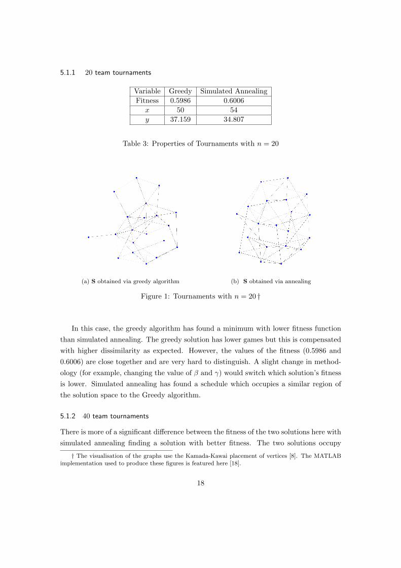
5.1.1 20 team tournaments

Variable Greedy Simulated Annealing

Fitness 0.5986 0.6006

x 50 54

y 37.159 34.807

Table 3: Properties of Tournaments with n = 20

(a) S obtained via greedy algorithm (b) S obtained via annealing

Figure 1: Tournaments with n = 20 †

In this case, the greedy algorithm has found a minimum with lower fitness function

than simulated annealing. The greedy solution has lower games but this is compensated

with higher dissimilarity as expected. However, the values of the fitness (0.5986 and

0.6006) are close together and are very hard to distinguish. A slight change in method-

ology (for example, changing the value of β and γ) would switch which solution’s fitness

is lower. Simulated annealing has found a schedule which occupies a similar region of

the solution space to the Greedy algorithm.

5.1.2 40 team tournaments

There is more of a significant difference between the fitness of the two solutions here with

simulated annealing finding a solution with better fitness. The two solutions occupy

† The visualisation of the graphs use the Kamada-Kawai placement of vertices [8]. The MATLABimplementation used to produce these figures is featured here [18].

18

Variable Greedy Simulated Annealing

Fitness 0.5962 0.5461

x 347 286

y 67.616 80.498

Table 4: Properties of Tournaments with n = 40

(a) S obtained via greedy algorithm (b) S obtained via annealing

Figure 2: Tournaments with n = 40

different areas of solution space with the greedy solution having 61 more games than the

annealed solution as opposed to the 20 team case where both solutions were similar in

fitness, the number of games and D. This implies the parameter values in the annealing

schedule in this case were maybe more appropriate than in the 20 team case.

We calculate the 20 and 40 team cases to explore whether there exists scaling with

respect to n in the properties of a tournament. All the tournaments have similar fitness.

However, comparing the visualisations of graphs, the number of games and D, there

does not appear to be any sign of scaling. The solution space has a lot of local minima

so it is not suprising the algorithms found schedules with different properties but similar

fitness function values.

5.1.3 120 team tournaments

We use data from the NCAA FBS season 2009-2010 [7]. The data includes the date,

the participants and the score of every college football match in 2009. As discussed in

Section 2.2, the FBS contains 120 teams but a hypothetical 121st is added to represent

19

all “non-FBS” teams in the random walker ranking system. However, for the purposes

of creating a FBS schedule, the possibility of FBS teams playing non-FBS teams is

excluded. We also only include the regular season as we seek to produce a ranking to

decide bowl match-ups. Hence, we filter out all matches violating these criteria. To

create the S matrix, we assign integers to each of the teams in FBS. The matrix S is

then created in the usual way: Sij = Sji = 1 if team i played team j and 0 otherwise.

We run the permutation procedure described in section 4.2 on page 12 to the get results

in Table 5.

Variable Greedy Simulated Anneal Actual

Fitness 0.5812 0.56667 0.3974

x 3500 3374 679

y 324.545 336.599 1030.267

Table 5: Properties of Tournaments with n = 120

20

(a) S obtained via greedy algorithm (b) S obtained via annealing

(c) S obtained from NCAA FBS Season 2009

Figure 3: Tournaments with n = 120

The simulated annealing and the greedy solutions have similar properties in terms

of fitness, number of games and dissimilarity. The simulated annealing solution has 126

fewer games but this is offset by an increased D of 12.054. These two solutions occupy a

similar region of the solution space. We observe that the actual schedule has significantly

better fitness than the other two tournaments. It has a much lower number of games

( 679, which is around 5 times lower) but higher D (1030.267, which is around 3 times

more). We believe this solution lies in a completely different area of solution space,

which has not been explored by the greedy algorithm or simulated annealing.

21

6 Conclusion

In this dissertation, we considered the Random Walker Ranking Algorithm, originally

expressed in terms of ordinary differential equations. We re-expressed this algorithm in

terms of Markov chains, in cases where the time for the hypothetical voter to decide on

its choice of the strongest team was continuous and discrete. We showed that the results

obtained from these three approaches are identical. We considered a partial ranking of

n teams as a bucket ordering on the set of n teams. A proper ranking (i.e. without ties)

has every bucket of size 1. We used Spearman’s Footrule, D to measure how dissimilar

two (partial) rankings are. Under the choice of the sure-win rule, we showed a robin-

robin has the lowest possible dissimilarity, D = 0. We searched for the worst possible

case of D, which we believe to occur when the smallest number of games (n − 1) has

been played. Hence, we used the Greedy Algorithm and Simulated Annealing to search

through the set of all trees on n vertices. To get an exact value for D required generating

n! permutations, which is prohibitively large. Thus, we used Monte Carlo methods to

calculate D. We defined a fitness function for a general schedule with n teams. We used

the same algorithms as before to search the set of all connected graphs on n vertices to

find a schedule with low fitness, with n set to 20, 40 and 120. We found no evidence of

scaling in schedules found in the 20 and 40 team case. In 120 team case, we compared

the algorithmic schedules with the 2009 schedule. The 2009 schedule had significantly

lower fitness rating implying it lies in a promising area of solution space, not explored

by either algorithm.

Possible areas for future work include understanding why neither algorithm found a

solution with fitness as good as the 2009 schedule. In the case of simulated annealing,

this could be down to the parameter choice or the “nearby” solution generator. Using

more computational power than was available for this dissertation, a more through

search of the solution space could be carried out (e.g. increasing nmax, the maximum

temperatures considered or K, number of solutions generated for each temperature),

which may yield better results. A solution generator that allowed a more effective

traversing of the solution space (set of all connected graphs on n vertices) would also

be an improvement. Alternatively, other optimisation heuristics may be more effective

at solving this problem. One could try an implementation of the genetic algorithm

approach, where a population of possible solutions are maintained. At each generation,

the solutions with the best fitness in the population pass on their characteristics to the

next generation. Over time, the solutions “evolve” towards the optimum solution.

In conclusion, the current FBS schedule provides a good tourament for use with the

22

Random Walker Ranking system. As we search for better tournaments, our understand-

ing of sports scheduling with respect to ranking algorithms will be improved.

References

[1] B. Bollobas. Modern graph theory. Springer Verlag, 1998.

[2] T. Callaghan, P. Mucha, and M. Porter. The bowl championship series: A mathe-

matical review. Arxiv preprint physics/0403049, 2004.

[3] T. Callaghan, P. Mucha, and M. Porter. Random walker ranking for NCAA division

IA football. American Mathematical Monthly, 114(9):761, 2007.

[4] P. Diaconis and R. Graham. Spearman’s Footrule as a Measure of Disarray. Journal

of the Royal Statistical Society. Series B (Methodological), page 262, 1977.

[5] R. Fagin, R. Kumar, M. Mahdian, D. Sivakumar, and E. Vee. Comparing and

aggregating rankings with ties. In Proceedings of the twenty-third ACM SIGMOD-

SIGACT-SIGART symposium on Principles of database systems, page 47, 2004.

[6] G. Grimmett and D. Stirzaker. Probability and random processes. Oxford University

Press, 2001.

[7] J. Howell. James howell’s college football scores, 2009.

[8] T. Kamada and S. Kawai. An algorithm for drawing general undirected graphs.

Information processing letters, 31(1):7, 1989.

[9] J. Keener. The Perron-Frobenius theorem and the ranking of football teams. SIAM

review, 35(1):80–93, 1993.

[10] K. Kobayashi, H. Kawasaki, and A. Takemura. Parallel matching for ranking all

teams in a tournament. Adv. in Appl. Probab, 38(3):804, 2006.

[11] B. P. League. Premier league rules 09/10, 2009.

[12] T. McGarry and R. Schutz. Efficacy of traditional sport tournament structures.

The Journal of the Operational Research Society, 48(1):65, 1997.

[13] J. Norris. Markov chains. Cambridge University Press, 1998.

[14] I. A. of Athletics Federations. Iaaf competition rules 2010-2011, 2010.

23

[15] B. Oommen and D. Ng. On generating random permutations with arbitrary distri-

butions. The Computer Journal, 33(4):368, 1990.

[16] G. Pollard. A new tennis scoring system. Res Q Exerc Sport, 58:229–233, 1987.

[17] W. Press, S. Teukolsky, W. Vetterling, and B. Flannery. Numerical recipes: the art

of scientific computing. Cambridge Univ Pr, 2007.

[18] A. Traud, C. Frost, P. Mucha, and M. Porter. Visualization of communities in

networks. Chaos: An Interdisciplinary Journal of Nonlinear Science, 19:041104,

2009.

[19] S. Young. Alternative aspects of sports scheduling. Preprint, 2004.

24