Optimising Cuts for HLT

George TalbotSupervisor: Stewart Martin-Haugh

ID HLT Tracking

There are 3 most important aspects to the ID HLT:• The timing – average of 200-250 ms spent in HLT, the ID

requires the most CPU power• Efficiency – it needs to be efficient to avoid losing good

tracks• Robustness – the code must behave correctly under all

conditionsThese become increasingly more difficult to maintain with increased hits in the ID as there become more possible combinations. This effect is non linear with more pileup

• This image gives an idea of the amount of data that is being reconstructed within the allotted time.

• In actuality there are far more tracks to test due to further pileup

Track Seeding and Track Finding

• Before cuts can be made the particle tracks first have to be identified.

• Detector is divided into slices in φ to work with• Also divided into areas known as Regions of Interest

(RoIs)• 3 spacepoints are matched up to create part of a track

known as a triplet. The parameters that define a triplet are pT, z0, d0, φ and η. Each triplet is then put through a monte carlo truth test to see if it matches up to the desired particle. If the triplet matches to truth then it is labelled ‘good’, if it matches to false then it is ‘bad’.

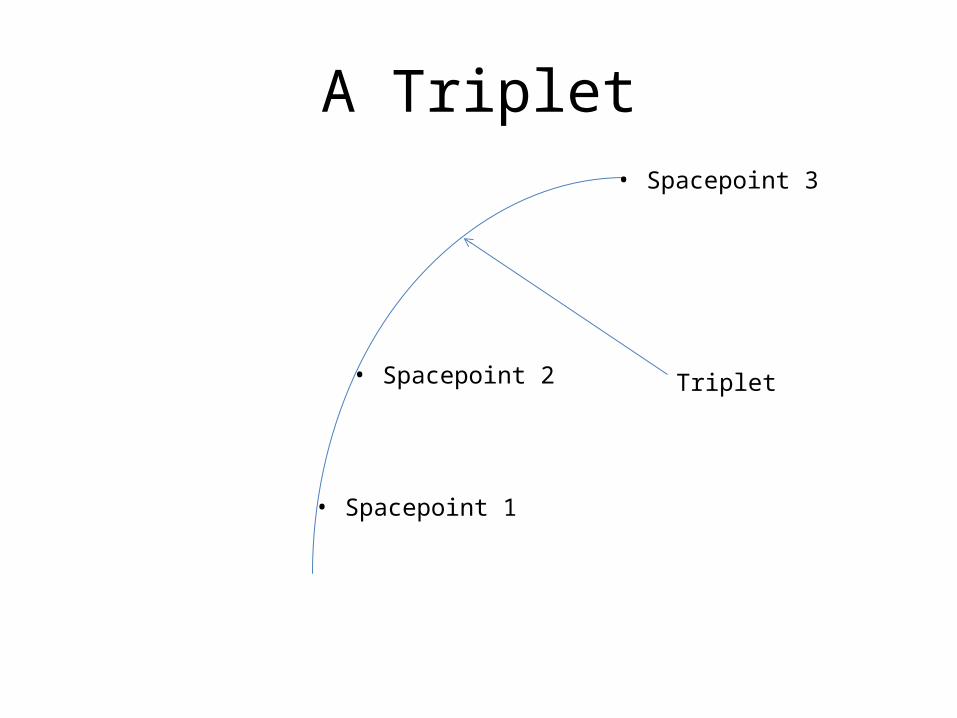
A Triplet

• Spacepoint 1

• Spacepoint 2

• Spacepoint 3

Triplet

The Cuts

• χ2 – a measure of the comparison of the expected errors and the true residuals for z and η

• rz – measure of how ‘straight’ the triplet is – there is no magnetic field in this plane (mm2)

• Δη – difference between η of observed triplet and η of RoI.

Setting Up

• Created an analysis code to book histograms and graphs by reading output from Athena job

• Wrote code to vary the cut values to test for the best compromise between efficiency and rejection

• Created a plot code which takes the booked histograms and graphs and plots them, outputting the results as pngs

Samples Used

• Started working with the single electron sample without pileup

• Later moved onto a sample containing pileup• Currently working on a new seeding method• None of the samples I have worked with have

contained the IBL

Histograms for Good vs Bad TripletsΔη is an example of a cut that was shown to be possibly too loose, resulting in unnecessary time spent in the cutting algorithm

rz is cut differently for Pixel (cut at 1) and SCT (cut at 8) detectors. This is because there are far larger errors in the SCT due to material effects and measurement errors. A cut of 8 for the SCT detectors in the Endcap looks as if it may be too tight, resulting in a loss of good triplets and therefore potentially interesting physics.

χ2 Probability

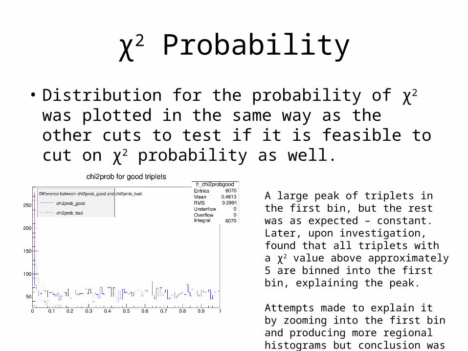
• Distribution for the probability of χ2 was plotted in the same way as the other cuts to test if it is feasible to cut on χ2 probability as well.

A large peak of triplets in the first bin, but the rest was as expected – constant. Later, upon investigation, found that all triplets with a χ2 value above approximately 5 are binned into the first bin, explaining the peak.

Attempts made to explain it by zooming into the first bin and producing more regional histograms but conclusion was that it cannot feasibly be cut on.

Efficiency and Rejection

• Graphs of efficiency vs rejection and efficiency and rejection as a function of cut value are a good way of looking for ways to optimise a cut value.

• All of these plots were put on the same canvas so that the information could be viewed at the same time

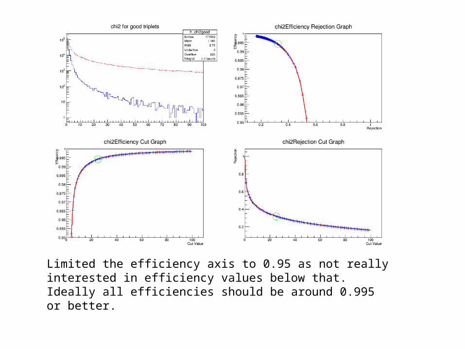
Limited the efficiency axis to 0.95 as not really interested in efficiency values below that. Ideally all efficiencies should be around 0.995 or better.

η Discrimination• Plots for χ2 and rz were split into regions of different η to test for the effects of

multiple Coulomb scattering – where electrons scatter off atoms. This is affected by the amount of material it has to pass through and how fast it is going

• Most material is in the region 1<η<2, and the slowest electrons are typically found at the lowest η.

Ref: The ATLAS Experiment at the CERN Large Hadron Collider, ATLAS Collaboration, 2008, page 107

The equation for multiple Coulomb scattering is:

Where θ0 is the angle scattered through, the units of 13.6 is MeV, p is the momentum, x is the distance travelled, X0 is the radiation length and the log term is usually taken as negligible and therefore ignored.

χ2 cut seemed to be least efficient in the region 1<η<2

The rz cut for the SCT showed as equally as inefficient for η>2

χ2 vs Momentum

• Plotting χ2 as a function of absolute momentum, which can be calculated from η and pT, is another indication of the effects of multiple scattering

• If multiple scattering has not been accounted for then it would be expected to see a larger distribution of χ2 around smaller momentum values

• Plotted χ2 vs momentum for the original code, and then for the code with a section included to account for multiple scattering, to see how well it works.

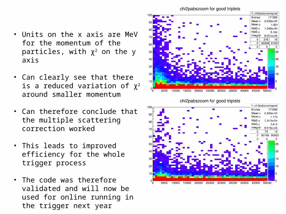
• Units on the x axis are MeV for the momentum of the particles, with χ2 on the y axis

• Can clearly see that there is a reduced variation of χ2 around smaller momentum

• Can therefore conclude that the multiple scattering correction worked

• This leads to improved efficiency for the whole trigger process

• The code was therefore validated and will now be used for online running in the trigger next year

Current Work

• Currently working on producing graphs and histograms for a completely new track seeding created by Dmitry.

• Will hopefully show better results than the old seeding

Any Questions?

Chi2 Discrimination (backup)

• Histograms produced for triplets with a chi2 of above 5 to test for triplets in the first bin

• No real light shed on cut-able distributions

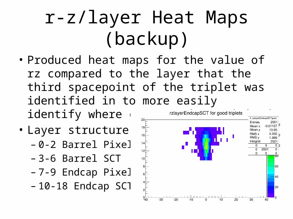
r-z/layer Heat Maps (backup)

• Produced heat maps for the value of rz compared to the layer that the third spacepoint of the triplet was identified in to more easily identify where cuts can be optimised

• Layer structure:– 0-2 Barrel Pixel– 3-6 Barrel SCT– 7-9 Endcap Pixel– 10-18 Endcap SCT

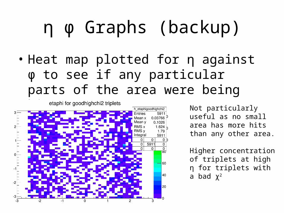
η φ Graphs (backup)

• Heat map plotted for η against φ to see if any particular parts of the area were being hit

Not particularly useful as no small area has more hits than any other area.

Higher concentration of triplets at high η for triplets with a bad χ2