Optimization Algorithms for RealizableSignal-Adapted Filter Banks

Thesis by

Andre Tkacenko

In Partial Fulfillment of the Requirements

for the Degree of

Doctor of Philosophy

California Institute of Technology

Pasadena, California

2004

(Submitted May 12, 2004)

ii

c© 2004

Andre Tkacenko

All Rights Reserved

iii

Acknowledgements

First of all, I would like to thank my advisor, Prof. P. P. Vaidyanathan, for the guidance he has given

me and for supporting me during my stay at Caltech. I first met P. P. when I was an undergrad at

Caltech, when he was assigned to be my advisor. Even though he was rather busy on account of

his Option Representative duties at the time, he was always there when I needed to see him and

attentative when I spoke with him. My respect for him grew when I took his course on digital signal

processing, EE 112. He was always able to take a daunting and difficult to understand concept and

simplify it and make it unintimidating. I was so grateful the day that P. P., after finishing his EE

112 lecture for the day, told me that I had been admitted to his group. As my graduate advisor,

he was always there for me and had my best interests at heart. He always pointed me in the right

direction when I was lost and supported me when I was on the right path. In addition to being my

mentor, he has also been a good friend to me. He has a good sense of humor and often times we

have exchanged jokes. (In addition to our love for digital signal processing and our sense of humor,

P. P. and I also have something else in common: a love for Three’s Company!) I will always be

grateful for the opportunity that he gave me to teach the multirate part of his signal processing

course, EE 112b, in the spring of 2003. Because of him, I aspire to return to academia some day.

I would like to thank the National Science Foundation (NSF) and the Office of Naval Research

(ONR) for financially supporting as a graduate student at Caltech. Also, I would like to thank

the members of my defense and candidacy examining committees: Prof. Robert J. McEliece, Prof.

Babak Hassibi, Prof. Jehoshua Bruck, Dr. Bojan Vrcelj, Dr. Payman Arabshahi, and Prof. Joel N.

Franklin. In particular, I would like to thank Prof. McEliece (The Chief) for being my teacher,

senior thesis advisor as an undergrad, and good friend. He was always willing to lend an ear to my

social travails and offer me good advise on what to do. Though his advise was always sagacious,

I unfortunately rarely followed it on account of my being young and naive. I would like to thank

him for his advise and friendship by taking him out to a certain restaurant again some time! In

addition to the above people, I would like to thank some of my teachers at Wilcox High School

iv

including Al Holland, my calculus teacher, and my gym teacher Jerry Louderback, whose wife was

able to procure a Caltech undergraduate application form for me at the proverbial eleventh hour.

I would like to thank my lab mates Bojan Vrcelj, Sony Akkarakaran, Murat Mese, Byung-Jun

Yoon, Sriram Murali, Mike Larsen, and Borching Su for making my time spent in the lab cheerful

and fun. My senior lab mates, Bojan, Sony, and Murat, were inspirational to me and helped me

mature from the first year graduate student that I once was to the senior leveled one that I am

now. In particular, I would especially like to thank Bojan for being both my friend and an elderly

brother figure for me. I miss our afternoon trips to Starbucks in Old Town Pasadena where we used

to sit, chat, and ogle at all of the pretty girls as they walked by. With any luck, I hope we will be

able to resume our old tradition once again. In addition, I would also like to thank Prof. Shayan

Mookherjea, my old friend from my undergraduate days at Caltech. I want to thank Shayan for

walking with me to all of those restaurants we used to eat at before any of us had cars and also

for introducing me to LATEX. Also, I want to thank Aristotelis Asimakopoulous, and friend of mine

from my undergraduate days who came back to Caltech during my graduate studies. He was my

partner in crime in various nefarious activities which I elect to omit here.

Also, I would like to thank my parents, Dusanka and Nikola Tkacenko, for their endless love

and support. I am indebted to them for the sacrifices that they made to put me through school

as an undergraduate. It is my hope that some day I will be able to be as good of a parent to my

children as my parents have been to me. I want to thank my brothers Nick, Boris, and Aleks for

being the best siblings that I could hope for. In particular, I want to thank my brother Nick for

being my best friend (and for introducing me to Buffy and Angel). I hope that we will be able

to spend more time with each other after he finishes school at UC Santa Cruz. Furthermore, I

would also like to thank my grandparents, Sofija and Nikola Milunovic, for their love and support.

In particular, I want to thank my grandfather Nikola, who is a master woodcarver, for offering to

carve me a throne for completing my doctorate. As with all of his other works, I am sure that it is

the “only one kind on planet [sic]”.

I would like to give a special thanks to my Princessa Victoria Delgadillo. She came into my life

when I least expected it and most needed it. It is because of her that I know what it is to feel alive.

She has been a light in my darkness and has shown me true happiness. I want to thank her for

loving me and supporting me during this tumultuous time in my life. Though I don’t know what

the future may hold for us, I want her to know that I love her and that she will always be a part

of my heart and my soul, now and forever.

v

Last, but certainly not least, I would like to thank God, the Infinite Being, for creating this

beautiful world in which we all live and beautiful mathematics (some of which I will present here in

my thesis). I also want to thank Him for always watching over me and protecting me (even when

I didn’t deserve it). Whenever I put my faith in His will, He always led me on the right path. I

pray that His love and divine presence will be with us all, now and ever, and unto the ages of ages.

Amen.

vi

Abstract

Multirate filter banks are fundamental systems commonly used in digital signal processing (DSP).

Typically, they are used to decompose a discrete-time signal into a set of frequency selective compo-

nents called subband signals. Filter banks have been found to be useful for lossy data compression

schemes such as MP3 and JPEG 2000, denoising, and signal estimation. In the last decade, trans-

multiplexers, the dual structures of multirate filter banks, have been shown to be useful in digital

communications systems such as discrete multitone (DMT) systems for channel equalization and

inter/intra-symbol interference cancellation in the presence of noise.

Recently, a special type of filter bank adapted to its input known as the principal component

filter bank (PCFB) has been shown to be simultaneously optimal for a wide variety of objectives.

Such filter banks are not only optimal for relevant data compression type objectives such as cod-

ing gain and multiresolution, but also for digital communications type objectives such as power

minimization, when the filter bank is implemented in its transmultiplexer form. The only problem

is that PCFBs, which are defined over classes of paraunitary (PU) filter banks, are only known

to exist for certain classes. In particular, PCFBs are in general known to exist only in the ex-

tremal cases where the analysis/synthesis polyphase matrix has zero memory and doubly infinite

memory, respectively. Furthermore, for many practical cases of inputs, the filters corresponding

to the infinite-order PCFB have ideal bandpass response and are as such unrealizable. When the

polyphase matrix has finite memory or a finite impulse response (FIR), it is believed that PCFBs

do not exist, although this has not yet been formally proven in the literature.

The main contribution of this thesis is to bridge the gap between the zero memory PCFB and

the infinite-order one. To that end, a variety of methods for the design of realizable signal-adapted

FIR filter banks is presented. It is shown that a popular conventional method for designing signal-

adapted FIR PU filter banks, which only requires the design of an optimal FIR compaction filter,

is in fact not well suited for designing good filter banks due to the exponential complexity caused

by the nonuniqueness of the FIR compaction filter. To avoid this dilemma, we propose a method

vii

by which all of the filters are obtained together. In particular, the method consists of finding an

FIR PU least-squares approximant to the infinite-order PCFB polyphase matrix. Using an elegant

complete parameterization of FIR PU systems in terms of canonical building blocks, an iterative

greedy algorithm for solving the least-squares problem is presented. Simulation results provided

here show that as the order or memory of the signal-adapted FIR PU filter bank increases, the filter

bank behaves more and more like the infinite-order PCFB in terms of a variety of objectives included

coding gain, multiresolution, and power minimization. This serves to bridge the gap between the

zero memory and infinite memory PCFBs, which previously has not been done in the literature.

In addition to being useful for the design of PCFB-like FIR filter banks, the proposed iterative

algorithm can also be used for a variety of other design problems including the FIR PU interpolation

problem. Unlike the traditional FIR interpolation problem, whose solution is known in closed form,

the FIR PU interpolation problem is far more difficult and is in fact still open. Despite this, the

proposed algorithm can be used to find an approximant to an interpolant and sometimes even find

an interpolant, as we show here through simulations.

In the second part of the thesis, we focus on the design of realizable signal-adapted quantized

filter banks in which the filters are FIR but otherwise unconstrained. The filters are chosen to

minimize the mean-squared error of the output, which is shown to be equivalent to maximizing the

coding gain of the system. By alternately optimizing the analysis and synthesis filters, an iterative

greedy algorithm, different from that mentioned above, is proposed for the design of such filter

banks. Simulation results provided show that the filter banks designed exhibit performance close

to the information theoretic rate-distortion bound.

Finally, we show how some of the techniques used in the above iterative algorithms can be

used for the design of a channel shortening equalizer. Channel shortening equalizers, which arise

in the context of digital communications, have been found to be necessary for DMT systems such

as the digital subscriber loop (DSL) in which the channel impulse response must be shortened to

the length of the cyclic prefix. In particular, we show how the eigenfilter technique which is used

in the above-mentioned FIR PU iterative greedy algorithm, can be used for the design of a noise

optimized channel shortening equalizer. As opposed to other techniques, which require a Cholesky

decomposition of a certain matrix for every delay parameter considered, the proposed method is

lower in complexity in that it only requires a single such decomposition for all delay values. Despite

this significant decrease in complexity, it is shown through simulations that the equalizers designed

using this technique perform nearly optimally in terms of observed bit rate.

viii

Contents

Acknowledgements iii

Abstract vi

1 Introduction 1

1.1 Review of Multirate Systems . . . . . . . . . . . . . . . . . . . . . . . . . . . . . . . 2

1.1.1 Discrete-Time Signal Processing . . . . . . . . . . . . . . . . . . . . . . . . . 2

1.1.2 Fundamental Building Blocks . . . . . . . . . . . . . . . . . . . . . . . . . . . 3

1.1.3 Decimation/Interpolation Filter Systems . . . . . . . . . . . . . . . . . . . . . 7

1.1.3.1 Noble Identities . . . . . . . . . . . . . . . . . . . . . . . . . . . . . 8

1.1.3.2 Polyphase Decompositions . . . . . . . . . . . . . . . . . . . . . . . 8

1.1.4 Filter Banks and Transmultiplexers . . . . . . . . . . . . . . . . . . . . . . . . 11

1.1.4.1 Polyphase Representations of Uniform Systems . . . . . . . . . . . . 13

1.1.4.2 Biorthogonality and Orthonormality . . . . . . . . . . . . . . . . . . 14

1.2 Signal-Adapted Filter Banks . . . . . . . . . . . . . . . . . . . . . . . . . . . . . . . 15

1.2.1 Principal Component Filter Banks . . . . . . . . . . . . . . . . . . . . . . . . 17

1.2.1.1 Classes for Which PCFBs Are Known to Exist . . . . . . . . . . . . 18

1.2.1.2 Difficulties with the Class of FIR PU Systems . . . . . . . . . . . . 18

1.3 The FIR PU Interpolation Problem . . . . . . . . . . . . . . . . . . . . . . . . . . . . 19

1.4 The Channel Shortening Equalizer Problem . . . . . . . . . . . . . . . . . . . . . . . 20

1.5 Outline of the Thesis . . . . . . . . . . . . . . . . . . . . . . . . . . . . . . . . . . . . 21

1.5.1 Eigenfilter Design of Overdecimated Compaction Filter Banks (Chapter 2) . 21

1.5.2 Multiresolution Optimal FIR PU Filter Banks (Chapter 3) . . . . . . . . . . 22

1.5.3 Direct FIR PU Approximation of the PCFB (Chapter 4) . . . . . . . . . . . 23

1.5.4 Coding Gain Optimal FIR Filter Banks (Chapter 5) . . . . . . . . . . . . . . 24

ix

1.5.5 Eigenfilter Channel Shortening Equalizer for DMT Systems (Chapter 6) . . . 24

1.6 Notations . . . . . . . . . . . . . . . . . . . . . . . . . . . . . . . . . . . . . . . . . . 25

2 Eigenfilter Design of Overdecimated Compaction Filter Banks 26

2.1 Outline . . . . . . . . . . . . . . . . . . . . . . . . . . . . . . . . . . . . . . . . . . . 27

2.2 The Compaction Filter Problem . . . . . . . . . . . . . . . . . . . . . . . . . . . . . 27

2.2.1 Solution in the Unconstrained Order Case . . . . . . . . . . . . . . . . . . . . 29

2.2.1.1 Special Case of WSS Input . . . . . . . . . . . . . . . . . . . . . . . 29

2.2.2 Overview of Previous Work on FIR Compaction Filters . . . . . . . . . . . . 30

2.3 Energy Compaction Problem for Overdecimated Filter Banks . . . . . . . . . . . . . 32

2.3.1 Derivation of the Energy Compaction Problem . . . . . . . . . . . . . . . . . 33

2.3.2 Imposing the FIR Constraint on the Matrix F(z) . . . . . . . . . . . . . . . . 34

2.4 Iterative Eigenfilter Method for Solving the FIR Compaction Problem . . . . . . . . 36

2.4.1 Solution to the Iterative Linearized Optimization Problem . . . . . . . . . . . 38

2.5 Simulation Results . . . . . . . . . . . . . . . . . . . . . . . . . . . . . . . . . . . . . 39

2.6 Concluding Remarks . . . . . . . . . . . . . . . . . . . . . . . . . . . . . . . . . . . . 42

Appendix: Least-Squares Signal Model Approximation Problem . . . . . . . . . . . . . . . 43

Blocked Form of LTI Systems and Pseudocirculant Matrices . . . . . . . . . . . . . . 44

Least-Squares Approximation Problem - Deterministic Case . . . . . . . . . . . . . . 46

Least-Squares Approximation Problem - Stochastic Case . . . . . . . . . . . . . . . . 50

3 Multiresolution Optimal FIR PU Filter Banks 54

3.1 Outline . . . . . . . . . . . . . . . . . . . . . . . . . . . . . . . . . . . . . . . . . . . 55

3.2 Complete Parameterization of 1-D Causal FIR PU Systems . . . . . . . . . . . . . . 57

3.3 Least-Squares Design of FIR Magnitude Squared Nyquist Filters . . . . . . . . . . . 58

3.3.1 Solving the Least-Squares Optimization Problem Using the Method of La-

grange Multipliers . . . . . . . . . . . . . . . . . . . . . . . . . . . . . . . . . 59

3.3.1.1 Optimal Choice of u0 . . . . . . . . . . . . . . . . . . . . . . . . . . 59

3.3.1.2 Optimal Choice of vk . . . . . . . . . . . . . . . . . . . . . . . . . . 60

3.3.2 Iterative Gradient Optimization Algorithm . . . . . . . . . . . . . . . . . . . 62

3.3.3 Simulation Results for Designing FIR Compaction Filters . . . . . . . . . . . 63

3.4 Phase Feedback Modification for Improving Compaction Gain . . . . . . . . . . . . . 65

x

3.5 Design of Signal-Adapted FIR PU Filter Banks

Using a Multiresolution Criterion . . . . . . . . . . . . . . . . . . . . . . . . . . . . . 68

3.5.1 Application of the Factorization of FIR PU Systems to the MOC . . . . . . . 69

3.5.2 Algorithm for the Design of FIR PU Multiresolution Optimal

Filter Banks . . . . . . . . . . . . . . . . . . . . . . . . . . . . . . . . . . . . 72

3.6 Simulation Results for MOC Designed FIR PU Filter Banks . . . . . . . . . . . . . . 73

3.6.1 Coding Gain Results . . . . . . . . . . . . . . . . . . . . . . . . . . . . . . . . 73

3.6.2 Multiresolution Optimality Results . . . . . . . . . . . . . . . . . . . . . . . . 76

3.6.3 Noise Reduction Using Zeroth-Order Wiener Filters . . . . . . . . . . . . . . 76

3.6.4 Power Minimization for Nonredundant PU Transmultiplexers . . . . . . . . . 78

3.7 Concluding Remarks . . . . . . . . . . . . . . . . . . . . . . . . . . . . . . . . . . . . 79

4 Direct FIR PU Approximation of the PCFB 80

4.1 Outline . . . . . . . . . . . . . . . . . . . . . . . . . . . . . . . . . . . . . . . . . . . 81

4.2 The FIR PU Approximation Problem . . . . . . . . . . . . . . . . . . . . . . . . . . 82

4.2.1 Optimal Choice of U . . . . . . . . . . . . . . . . . . . . . . . . . . . . . . . . 83

4.2.2 Optimal Choice of vk . . . . . . . . . . . . . . . . . . . . . . . . . . . . . . . 85

4.2.3 Iterative Greedy Algorithm for Solving the Approximation Problem . . . . . 87

4.3 Phase Feedback Modification . . . . . . . . . . . . . . . . . . . . . . . . . . . . . . . 88

4.3.1 Phase-Type Ambiguity . . . . . . . . . . . . . . . . . . . . . . . . . . . . . . . 88

4.3.2 Derivation of the Phase Feedback Modification . . . . . . . . . . . . . . . . . 89

4.3.3 Greediness of the Phase Feedback Modification . . . . . . . . . . . . . . . . . 91

4.4 Simulation Results . . . . . . . . . . . . . . . . . . . . . . . . . . . . . . . . . . . . . 91

4.4.1 Design of PCFB-like FIR PU Filter Banks . . . . . . . . . . . . . . . . . . . . 91

4.4.1.1 Multiresolution Optimality Results . . . . . . . . . . . . . . . . . . . 93

4.4.1.2 Coding Gain Results . . . . . . . . . . . . . . . . . . . . . . . . . . . 97

4.4.1.3 Noise Reduction Using Zeroth-Order Wiener Filters . . . . . . . . . 98

4.4.1.4 Power Minimization for DMT-Type Transmultiplexers . . . . . . . . 98

4.4.2 The FIR PU Interpolation Problem . . . . . . . . . . . . . . . . . . . . . . . 100

4.4.2.1 FIR PU Interpolation - Example 1 . . . . . . . . . . . . . . . . . . . 101

4.4.2.2 FIR PU Interpolation - Example 2 . . . . . . . . . . . . . . . . . . . 102

4.5 Concluding Remarks . . . . . . . . . . . . . . . . . . . . . . . . . . . . . . . . . . . . 103

xi

5 Coding Gain Optimal FIR Filter Banks 104

5.1 Outline . . . . . . . . . . . . . . . . . . . . . . . . . . . . . . . . . . . . . . . . . . . 105

5.2 Uniform Quantized Filter Bank Model . . . . . . . . . . . . . . . . . . . . . . . . . . 106

5.3 Optimizing the Mean-Squared Reconstruction Error . . . . . . . . . . . . . . . . . . 108

5.3.1 Optimal Synthesis Bank F(z) for Fixed Analysis Bank H(z) . . . . . . . . . 110

5.3.2 Optimal Analysis Bank H(z) for Fixed Synthesis Bank F(z) . . . . . . . . . 111

5.3.2.1 Simplifying the Quantization Noise Term . . . . . . . . . . . . . . . 111

5.3.2.2 Imposing the FIR Constraint on H(z) . . . . . . . . . . . . . . . . . 112

5.3.3 Iterative Greedy Analysis/Synthesis Filter Bank Optimization Algorithm . . 115

5.4 Simulation Results . . . . . . . . . . . . . . . . . . . . . . . . . . . . . . . . . . . . . 116

5.4.1 Overdecimated Filter Bank Design . . . . . . . . . . . . . . . . . . . . . . . . 116

5.4.1.1 Single Subband Design Example . . . . . . . . . . . . . . . . . . . . 116

5.4.1.2 Multiple Subband Design Example . . . . . . . . . . . . . . . . . . . 119

5.4.2 Quantized Filter Bank Design . . . . . . . . . . . . . . . . . . . . . . . . . . . 122

5.4.2.1 Single Channel Example - Pre/Postfiltering in Quantization . . . . 124

5.4.2.2 Maximally Decimated Quantized Filter Bank . . . . . . . . . . . . . 129

5.5 Concluding Remarks . . . . . . . . . . . . . . . . . . . . . . . . . . . . . . . . . . . . 133

6 Eigenfilter Channel Shortening Equalizer for DMT Systems 134

6.1 Outline . . . . . . . . . . . . . . . . . . . . . . . . . . . . . . . . . . . . . . . . . . . 134

6.2 The Channel Shortening Equalizer Problem . . . . . . . . . . . . . . . . . . . . . . . 135

6.2.1 Overview of Previous Work on Channel Shortening Equalizers . . . . . . . . 138

6.3 Proposed Eigenfilter Design Method . . . . . . . . . . . . . . . . . . . . . . . . . . . 141

6.3.1 Analysis of the Objective Function J . . . . . . . . . . . . . . . . . . . . . . . 143

6.4 Simulation Results . . . . . . . . . . . . . . . . . . . . . . . . . . . . . . . . . . . . . 145

6.5 Concluding Remarks . . . . . . . . . . . . . . . . . . . . . . . . . . . . . . . . . . . . 148

Appendix: Equivalence between FSEs and the SIMO-MISO Channel/Equalizer Model . . 148

7 Conclusion 151

7.1 Open Problems . . . . . . . . . . . . . . . . . . . . . . . . . . . . . . . . . . . . . . . 152

Bibliography 154

xii

List of Figures

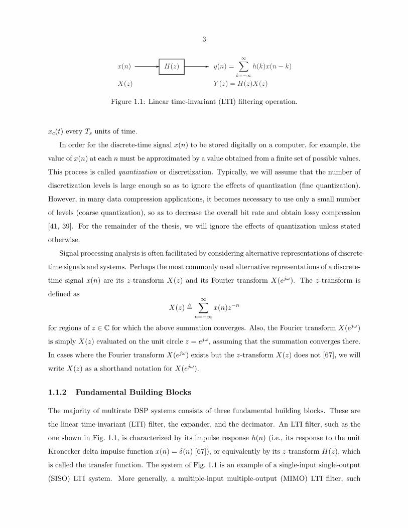
1.1 Linear time-invariant (LTI) filtering operation. . . . . . . . . . . . . . . . . . . . . . . 3

1.2 Multiple-input multiple-output (MIMO) LTI filtering operation. . . . . . . . . . . . . 4

1.3 L-fold expander input/output relationship: (a) Block diagram, (b) Example for L = 2. 4

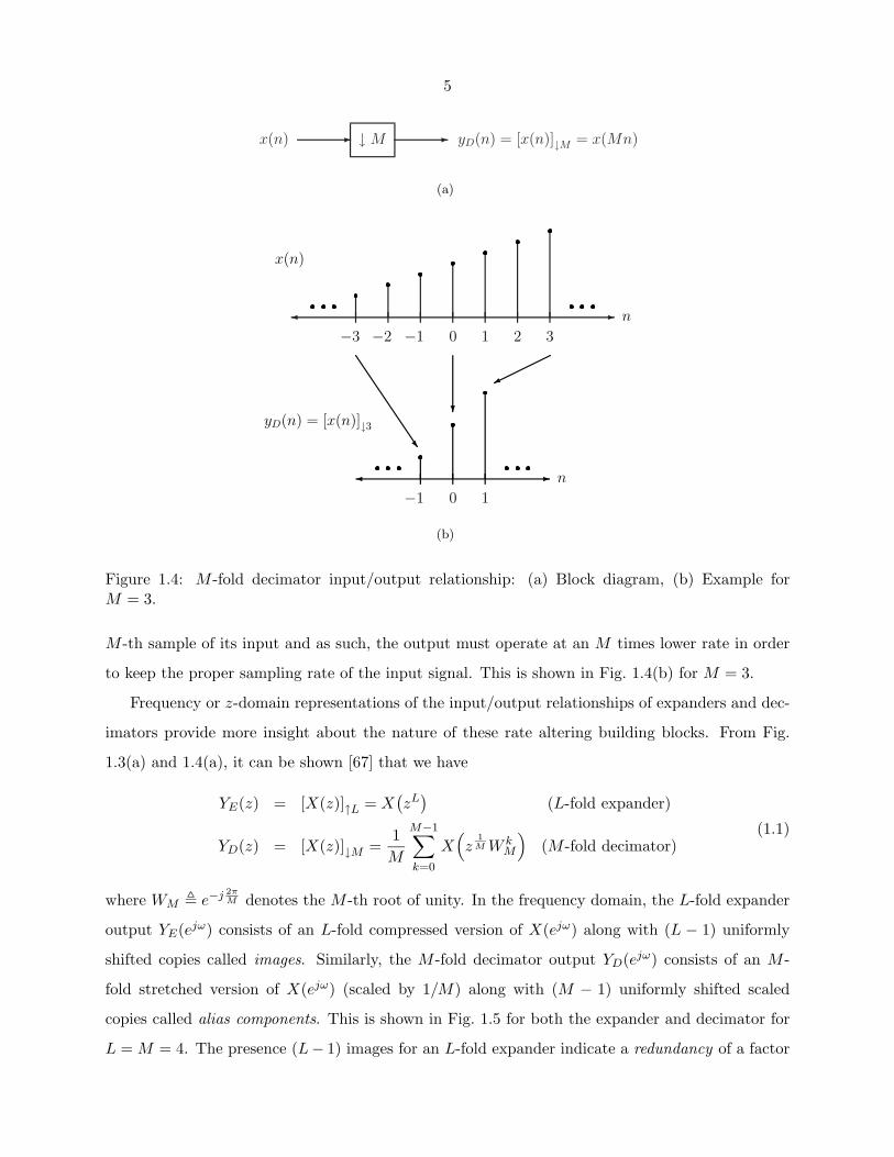
1.4 M -fold decimator input/output relationship: (a) Block diagram, (b) Example for

M = 3. . . . . . . . . . . . . . . . . . . . . . . . . . . . . . . . . . . . . . . . . . . . . 5

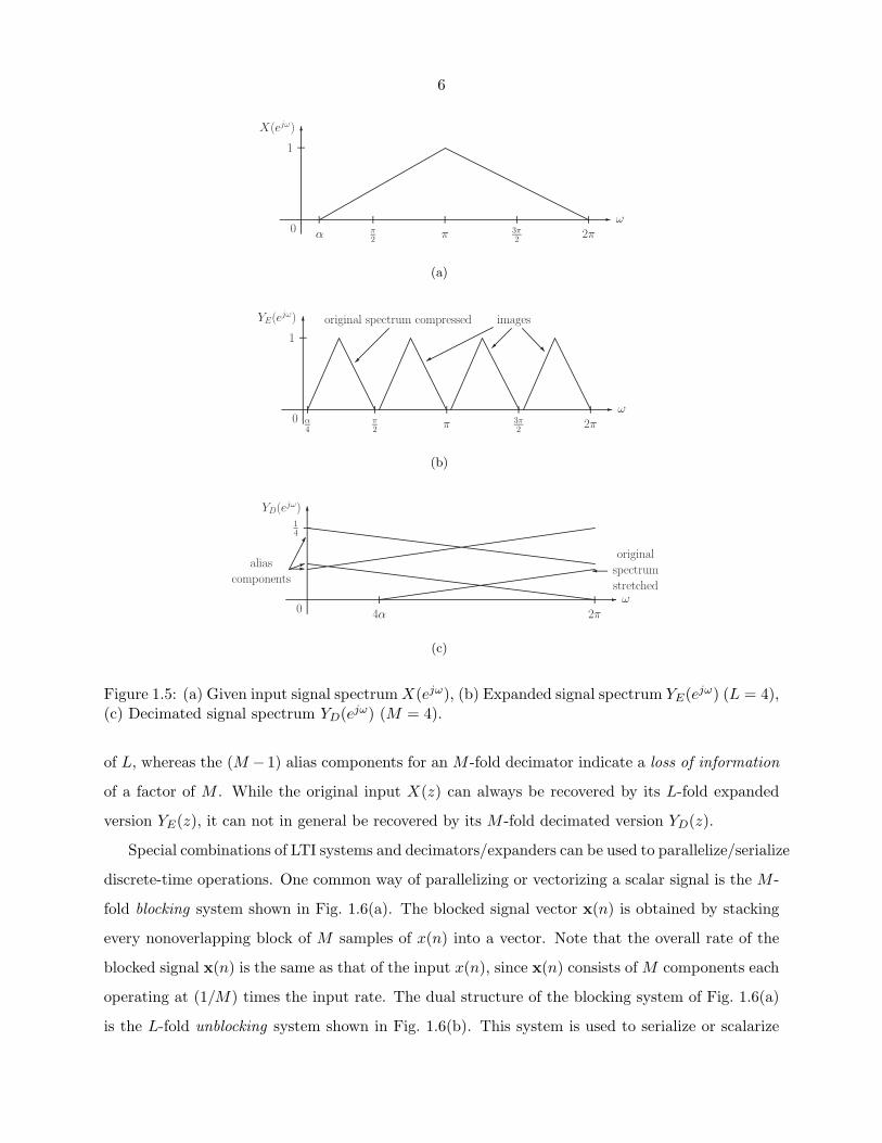
1.5 (a) Given input signal spectrum X(ejω), (b) Expanded signal spectrum YE(ejω) (L =

4), (c) Decimated signal spectrum YD(ejω) (M = 4). . . . . . . . . . . . . . . . . . . . 6

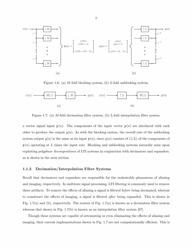
1.6 (a) M -fold blocking system, (b) L-fold unblocking system. . . . . . . . . . . . . . . . . 7

1.7 (a) M -fold decimation filter system, (b) L-fold interpolation filter system. . . . . . . . 7

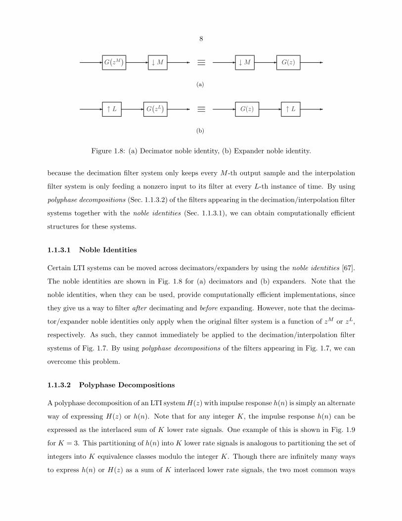
1.8 (a) Decimator noble identity, (b) Expander noble identity. . . . . . . . . . . . . . . . . 8

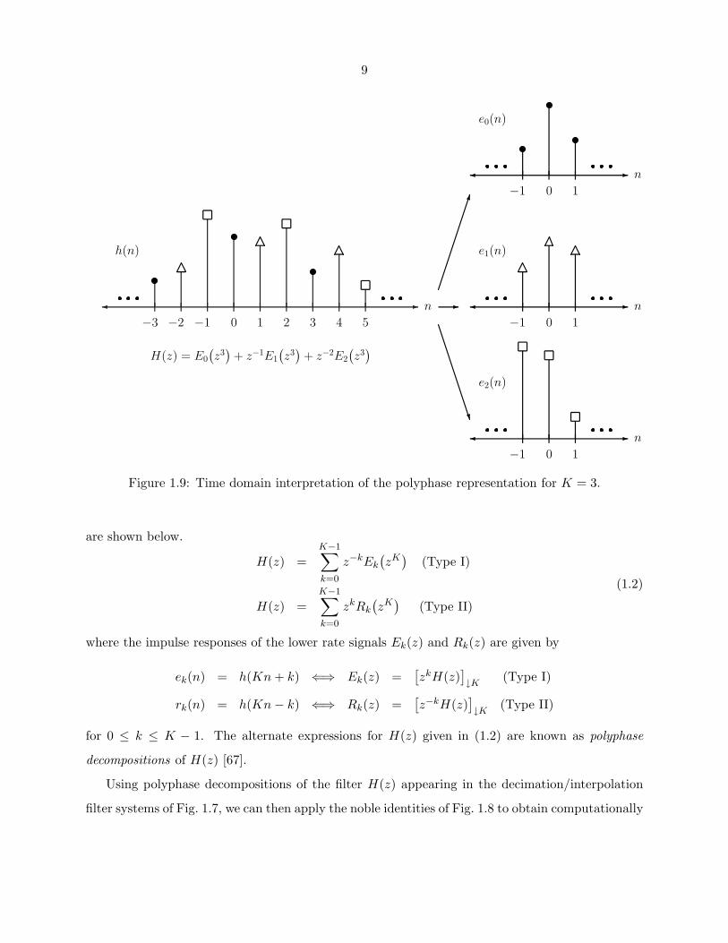
1.9 Time domain interpretation of the polyphase representation for K = 3. . . . . . . . . 9

1.10 Polyphase implementations of (a) decimation filter system (using (1.3)), (b) interpo-

lation filter system (using (1.4)). . . . . . . . . . . . . . . . . . . . . . . . . . . . . . . 10

1.11 (a) General nonuniform multirate filter bank, (b) The dual structured transmultiplexer. 11

1.12 Polyphase representations of (a) uniform filter bank, (b) uniform transmultiplexer. . . 13

1.13 (a) Typical uniform M -channel maximally decimated filter bank system. (b) Polyphase

representation of the filter bank. . . . . . . . . . . . . . . . . . . . . . . . . . . . . . . 16

1.14 Typical discrete multitone (DMT) system. . . . . . . . . . . . . . . . . . . . . . . . . 20

1.15 Channel shortening equalizer model. . . . . . . . . . . . . . . . . . . . . . . . . . . . . 21

2.1 (a) One-channel overdecimated filter bank model. (b) Polyphase implementation. . . . 28

2.2 (a) Uniform overdecimated filter bank (L < M), (b) Polyphase representation. . . . . 32

2.3 Input power spectral density Sxx(ejω). . . . . . . . . . . . . . . . . . . . . . . . . . . . 39

2.4 Orthonormality error ||εk||F vs. the iteration index k (L = 1, M = 7). . . . . . . . 40

xiii

2.5 Magnitude squared responses of the designed FIR synthesis filter F0(z) along with the

first filter of the infinite-order PCFB (L = 1, M = 7). . . . . . . . . . . . . . . . . . . 40

2.6 Compaction gain Gcomp vs. the filter order parameter N . . . . . . . . . . . . . . . . . 41

2.7 Orthonormality error ||εk||F vs. the iteration index k (L = 2, M = 7, N = 10). . . . . 42

2.8 Magnitude squared responses of the designed FIR synthesis filters F0(z) and F1(z)

along with the first two filters of the infinite-order PCFB (L = 2, M = 7, N = 10). . . 42

2.9 Rational nonuniform synthesis bank. . . . . . . . . . . . . . . . . . . . . . . . . . . . . 44

2.10 (a) Decimator/expander cascade identity, (b) Polyphase identity. . . . . . . . . . . . . 45

2.11 M -fold blocked form of an LTI system H(z). . . . . . . . . . . . . . . . . . . . . . . . 45

2.12 (a) The k-th branch of the signal model from Fig. 2.9, (b) With Fk(z) implemented in

an mkN -fold block form, (c) Resulting structure after applying the polyphase identity. 48

2.13 System for obtaining the optimal driving signal C(z). . . . . . . . . . . . . . . . . . . 49

2.14 (a) Equivalent form of Fig. 2.9 with blocking/unblocking elements removed, (b) Method

for obtaining the optimal driving signal. . . . . . . . . . . . . . . . . . . . . . . . . . . 50

3.1 Input psd Sxx(ejω) and ideal compaction filter magnitude squared response∣∣D(ejω)

∣∣2for M = 3. . . . . . . . . . . . . . . . . . . . . . . . . . . . . . . . . . . . . . . . . . . 63

3.2 Mean-squared error ξm vs. the iteration index m. . . . . . . . . . . . . . . . . . . . . . 64

3.3 Magnitude squared responses of the ideal compaction filter D(ejω) and the designed

FIR compaction filter F (ejω). . . . . . . . . . . . . . . . . . . . . . . . . . . . . . . . . 64

3.4 Compaction gain Gcomp vs. the filter order parameter N . . . . . . . . . . . . . . . . . 65

3.5 Compaction gain Gcomp vs. the filter order parameter N using the phase feedback

modification. . . . . . . . . . . . . . . . . . . . . . . . . . . . . . . . . . . . . . . . . . 67

3.6 Compaction filter design using the phase feedback modification. (a) Mean-squared

error vs. iteration. (b) Magnitude squared response. . . . . . . . . . . . . . . . . . . . 67

3.7 Uniform M -channel maximally decimated PU filter bank. . . . . . . . . . . . . . . . . 68

3.8 Implementation of the analysis bank using the factorization of F(z) from (3.25). . . . 70

3.9 Observed coding gain Gcode as a function of the synthesis polyphase order N . . . . . . 73

3.10 Zero locations of the optimal spectral factor for N = 11. . . . . . . . . . . . . . . . . . 74

3.11 Analysis filter magnitude squared responses for the optimal spectral factor for N = 11.

(a) First channel. (b) Second channel. (c) Third channel. . . . . . . . . . . . . . . . . 75

xiv

3.12 Analysis filter magnitude squared responses for the minimum-phase spectral factor

for N = 11. (a) First channel. (b) Second channel. (c) Third channel. . . . . . . . . . 75

3.13 Proportion P (L) of the total variance as a function of the number of subbands kept

L for (a) N = 3 and (b) N = 9. . . . . . . . . . . . . . . . . . . . . . . . . . . . . . . . 76

3.14 Mean-squared error ε from (3.37) as a function of N for (a) η2 = 1 and (b) η2 = 4. . . 77

3.15 Uniform PU nonredundant transmultiplexer. . . . . . . . . . . . . . . . . . . . . . . . 78

3.16 Total required power P from (3.40) as a function of N . . . . . . . . . . . . . . . . . . 79

4.1 Input psd Sxx(ejω) of the AR(4) process x(n). . . . . . . . . . . . . . . . . . . . . . . 92

4.2 Mean-squared error ξm vs. iteration m for both the unmodified and phase feedback

modified iterative algorithms. (a) Plot of KN = 3, 000 iterations, (b) Magnified plot

of the first 20 iterations. . . . . . . . . . . . . . . . . . . . . . . . . . . . . . . . . . . . 93

4.3 Magnitude squared responses of the PCFB and FIR PU synthesis filters using the

unmodified iterative algorithm. (a) F0(z), (b) F1(z), (c) F2(z), (d) F3(z). . . . . . . . 94

4.4 Magnitude squared responses of the PCFB and FIR PU synthesis filters using the

phase feedback modified iterative algorithm. (a) F0(z), (b) F1(z), (c) F2(z), (d) F3(z). 95

4.5 Proportion of the total variance P (L) as a function of the number of subbands kept

L for an M = 4 channel system with (a) N = 3 and (b) N = 10. . . . . . . . . . . . . 96

4.6 Proportion of the total variance P (L) as a function of the number of subbands kept

L for an M = 8 channel system with (a) N = 3 and (b) N = 10. . . . . . . . . . . . . 97

4.7 Observed coding gain Gcode as a function of the FIR PU filter order parameter N . . . 98

4.8 Noise reduction performance (ε from (3.37)) with zeroth-order subband Wiener filters

as a function of the FIR PU filter order parameter N for (a) noise variance (η2) of 1

and (b) noise variance of 4. . . . . . . . . . . . . . . . . . . . . . . . . . . . . . . . . . 99

4.9 Nonredundant DMT-type transmultiplexer total required power P as a function of

the FIR PU filter order parameter N . . . . . . . . . . . . . . . . . . . . . . . . . . . . 100

4.10 FIR PU interpolation problem - Example 1: Mean-squared error ξm vs. iteration m. . 101

4.11 FIR PU interpolation problem - Example 2: Mean-squared error ξm vs. iteration m. . 102

5.1 (a) Uniform filter bank with scalar quantizers in the subbands, (b) Polyphase repre-

sentation of the filter bank. . . . . . . . . . . . . . . . . . . . . . . . . . . . . . . . . . 106

5.2 High bit rate quantizer model. . . . . . . . . . . . . . . . . . . . . . . . . . . . . . . . 107

5.3 Equivalent quantized filter bank model under the high bit rate assumption. . . . . . . 108

xv

5.4 Input psd Sxx(ejω) to the system of Fig. 5.1. . . . . . . . . . . . . . . . . . . . . . . . 116

5.5 Mean-squared reconstruction error ξk as a function of the iteration index k. (Single

subband example) . . . . . . . . . . . . . . . . . . . . . . . . . . . . . . . . . . . . . . 117

5.6 Magnitude squared responses of the analysis and synthesis filters for (a) Nf = Nh = 7

and (b) Nf = Nh = 10. (Single subband example) . . . . . . . . . . . . . . . . . . . . 118

5.7 Deviation from (a) orthonormality δ⊥,k and (b) biorthogonality δBIO,k as a function

of the iteration index k. (Single subband example) . . . . . . . . . . . . . . . . . . . . 119

5.8 Mean-squared reconstruction error ξk as a function of the iteration index k. (Multiple

subband example) . . . . . . . . . . . . . . . . . . . . . . . . . . . . . . . . . . . . . . 120

5.9 Deviation from (a) orthonormality δ⊥,k and (b) biorthogonality δBIO,k as a function

of the iteration index k. (Multiple subband example) . . . . . . . . . . . . . . . . . . 120

5.10 Magnitude squared responses of the analysis filters Hk(z) and synthesis filters Fk(z)

for (a) k = 0, and (b) k = 1. (Multiple subband example) . . . . . . . . . . . . . . . . 121

5.11 Equivalent overdecimated filter bank model in the absence of quantizers. . . . . . . . 122

5.12 Pre/postfiltering quantization system. . . . . . . . . . . . . . . . . . . . . . . . . . . . 124

5.13 Mean-squared reconstruction error ξk as a function of the iteration index k for (a)

N = 10 and (b) N = 20. . . . . . . . . . . . . . . . . . . . . . . . . . . . . . . . . . . . 125

5.14 Deviation from orthonormality δ⊥,k as a function of the iteration index k for (a)

N = 10 and (b) N = 20. . . . . . . . . . . . . . . . . . . . . . . . . . . . . . . . . . . . 126

5.15 Deviation from biorthogonality δBIO,k as a function of the iteration index k for (a)

N = 10 and (b) N = 20. . . . . . . . . . . . . . . . . . . . . . . . . . . . . . . . . . . . 126

5.16 Magnitude squared responses of the analysis filter H0(z) = H(z) and the synthesis

filter F0(z) = F (z) for (a) N = 10 and (b) N = 20. . . . . . . . . . . . . . . . . . . . . 127

5.17 Observed distortion DFB as a function of the average bit rate b plotted with the direct

quantization and rate-distortion bounds. . . . . . . . . . . . . . . . . . . . . . . . . . . 128

5.18 Observed coding gain Gcode as a function of the analysis/synthesis filter order N . . . . 128

5.19 Mean-squared reconstruction error ξk as a function of the iteration index k for (a)

N = 3 and (b) N = 6. . . . . . . . . . . . . . . . . . . . . . . . . . . . . . . . . . . . . 129

5.20 Deviation from orthonormality δ⊥,k as a function of the iteration index k for (a) N = 3

and (b) N = 6. . . . . . . . . . . . . . . . . . . . . . . . . . . . . . . . . . . . . . . . . 130

5.21 Deviation from biorthogonality δBIO,k as a function of the iteration index k for (a)

N = 3 and (b) N = 6. . . . . . . . . . . . . . . . . . . . . . . . . . . . . . . . . . . . . 130

xvi

5.22 Magnitude squared responses of the analysis and synthesis filters for N = 3. (a)

H0(z), F0(z), (b) H1(z), F1(z), (c) H2(z), F2(z). . . . . . . . . . . . . . . . . . . . . . 131

5.23 Magnitude squared responses of the analysis and synthesis filters for N = 6. (a)

H0(z), F0(z), (b) H1(z), F1(z), (c) H2(z), F2(z). . . . . . . . . . . . . . . . . . . . . . 131

5.24 Observed distortion DFB as a function of the average bit rate b plotted with (a) the

direct quantization and rate-distortion bounds, (b) the pre/postfiltering quantization

results. . . . . . . . . . . . . . . . . . . . . . . . . . . . . . . . . . . . . . . . . . . . . 132

5.25 Observed coding gain Gcode as a function of the analysis/synthesis polyphase filter

order N . . . . . . . . . . . . . . . . . . . . . . . . . . . . . . . . . . . . . . . . . . . . 133

6.1 Channel shortening equalizer model. . . . . . . . . . . . . . . . . . . . . . . . . . . . . 135

6.2 Decomposition of the effective channel ceff(n) into a desired channel cdes(n) and resid-

ual channel cres(n). . . . . . . . . . . . . . . . . . . . . . . . . . . . . . . . . . . . . . . 136

6.3 Discrete-time model of a K-fold oversampled FSE. . . . . . . . . . . . . . . . . . . . . 141

6.4 SIMO-MISO channel/equalizer model. . . . . . . . . . . . . . . . . . . . . . . . . . . . 141

6.5 Noise psd Sηη(ejω) corresponding to NEXT noise with eight disturbers [46] plus

AWGN with power density −110 dBm/Hz. . . . . . . . . . . . . . . . . . . . . . . . . 146

6.6 Original and equalized channel impulse responses using the proposed eigenfilter method

for CSA loop #1. . . . . . . . . . . . . . . . . . . . . . . . . . . . . . . . . . . . . . . 146

6.7 Observed bit rate (as a percentage of the MFB bit rate of (6.2)) as a function of the

tradeoff parameter α for CSA loop #1. . . . . . . . . . . . . . . . . . . . . . . . . . . 146

6.8 Equivalent form of Fig. 6.3 upon using the noble identities. . . . . . . . . . . . . . . . 149

6.9 Equivalent form of Fig. 6.8 upon moving the noise process η(n) past the blocking system.149

6.10 Equivalent form of Fig. 6.9 upon removing the unblocking/blocking systems. . . . . . 150

xvii

List of Tables

6.1 Observed bit rates for CSA loops #1-8 using various TEQ design methods. (Bit rates

are expressed as a percentage of the MFB maximum achievable bit rate of (6.2) for

each loop.) . . . . . . . . . . . . . . . . . . . . . . . . . . . . . . . . . . . . . . . . . . 147

1

Chapter 1

Introduction

Filter banks are common systems that arise in the study of multirate digital signal processing [67, 13]

and wavelet theory [32, 47]. Essentially, a multirate filter bank decomposes a given input signal

into a set of lower rate components known as subband signals. Often times, some subband signals

contain more information about the original input than others. In these cases, the subbands can be

easily manipulated to remove some of the redundancy present in the original input signal, resulting

in data compression. Popular lossy data compression schemes such as MP3 (for audio signals)

as well as JPEG and JPEG 2000 (for image signals) use filter banks in this manner to remove

the redundancy present in the original signals [41, 39]. In addition to this, transmultiplexers

[67], which are dual structures of multirate filter banks, have been found to be useful in digital

communications [46, 15, 16]. By adding a minimal amount of redundancy, transmultiplexers have

been found to be able to achieve stable blind channel equalization [14, 42, 43] and the removal of

inter/intra-symbol interference [17, 18] all in the presence of noise. Several well known modern

communications systems such as digital subscriber loop (DSL) and orthogonal frequency division

multiplexing (OFDM), which are examples of discrete multitone (DMT) systems [26], consist of

transmultiplexers with redundancy [46].

Recently, a special filter bank adapted to its input statistics known as the principal components

filter bank (PCFB) [62, 1, 69] has been found to be simultaneously optimal for a wide variety of

objectives. In particular, PCFBs are optimal for data compression type objectives such as coding

gain and multiresolution, as well as for digital communications type objectives such as power

minimization when the filter bank is implemented in its transmultiplexer form [1]. Unfortunately,

PCFBs, which are defined over classes of paraunitary (PU) filter banks, are in general only known to

exist for two special classes [1]. In particular, PCFBs are known to exist only in the extremal cases

where the filter bank analysis/synthesis polyphase matrix has zero memory and doubly infinite

2

memory, respectively. For many practical input signals, this latter class consists of filters that

have ideal bandpass characteristics and are as such unrealizable [68]. Though several methods

for the design of realizable signal-adapted filter banks have been proposed (see [35, 37, 79] for

example), none have established a connection between their filter banks and the unrealizable PCFB.

In particular, though we might expect a realizable filter bank of finite order that is optimized for

a particular objective to behave more and more like the unrealizable PCFB as the order increases,

this has not yet been shown in the literature.

The thesis presents several optimization algorithms for the design of realizable signal-adapted

filter banks in which the filters all have a finite impulse response (FIR). Matlab code for these

algorithms will soon be available at [60]. One of the main contributions is to establish a link between

realizable signal-adapted filter banks and the unrealizable infinite-order PCFB. In particular, it will

be shown that FIR filter banks designed using our methods behave more and more like the infinite-

order PCFB as the filter order increases. This serves to bridge the gap between the zero memory

PCFB and the infinite-order one which previously has not been done in the literature.

The primary purpose of this introductory chapter is to set the stage for the remainder of

the thesis. To that end, every attempt has been made to keep the chapter as self-contained as

possible. In this chapter, a brief overview of multirate systems and identities which will be used

throughout the thesis, as well as commonly used notations and terminology, is given in Sec. 1.1.

We formally introduce PCFBs in this chapter (Sec. 1.2.1) and mention problems related to them.

In addition, we discuss other problems relevant to the thesis including the FIR paraunitary (PU)

interpolation problem in Sec. 1.3 and the channel shortening equalizer problem in Sec. 1.4. The

material presented here is by no means a complete coverage of multirate systems and filter banks.

For a more comprehensive treatment of multirate system theory and its applications, the reader is

referred to [67, 32, 47, 41, 39, 15, 16].

1.1 Review of Multirate Systems

1.1.1 Discrete-Time Signal Processing

All of the signals of interest in DSP are discrete-time sequences of either real or complex numbers.

These sequences are typically obtained by uniformly sampling a continuous-time signal, such as a

voltage signal as a function of time. For example, if xc(t) denotes a continuous-time signal, then the

sequence x(n) � xc(nTs) for n ∈ Z denotes a discrete-time signal obtained by uniformly sampling

3

� H(z) �x(n)

X(z)

y(n) =∞∑

k=−∞h(k)x(n − k)

Y (z) = H(z)X(z)

Figure 1.1: Linear time-invariant (LTI) filtering operation.

xc(t) every Ts units of time.

In order for the discrete-time signal x(n) to be stored digitally on a computer, for example, the

value of x(n) at each n must be approximated by a value obtained from a finite set of possible values.

This process is called quantization or discretization. Typically, we will assume that the number of

discretization levels is large enough so as to ignore the effects of quantization (fine quantization).

However, in many data compression applications, it becomes necessary to use only a small number

of levels (coarse quantization), so as to decrease the overall bit rate and obtain lossy compression

[41, 39]. For the remainder of the thesis, we will ignore the effects of quantization unless stated

otherwise.

Signal processing analysis is often facilitated by considering alternative representations of discrete-

time signals and systems. Perhaps the most commonly used alternative representations of a discrete-

time signal x(n) are its z-transform X(z) and its Fourier transform X(ejω). The z-transform is

defined as

X(z) �∞∑

n=−∞x(n)z−n

for regions of z ∈ C for which the above summation converges. Also, the Fourier transform X(ejω)

is simply X(z) evaluated on the unit circle z = ejω, assuming that the summation converges there.

In cases where the Fourier transform X(ejω) exists but the z-transform X(z) does not [67], we will

write X(z) as a shorthand notation for X(ejω).

1.1.2 Fundamental Building Blocks

The majority of multirate DSP systems consists of three fundamental building blocks. These are

the linear time-invariant (LTI) filter, the expander, and the decimator. An LTI filter, such as the

one shown in Fig. 1.1, is characterized by its impulse response h(n) (i.e., its response to the unit

Kronecker delta impulse function x(n) = δ(n) [67]), or equivalently by its z-transform H(z), which

is called the transfer function. The system of Fig. 1.1 is an example of a single-input single-output

(SISO) LTI system. More generally, a multiple-input multiple-output (MIMO) LTI filter, such

4

H(z)r p

x(n)

X(z)

y(n) =∞∑

k=−∞h(k)x(n − k)

Y(z) = H(z)X(z)

Figure 1.2: Multiple-input multiple-output (MIMO) LTI filtering operation.

� ↑ L �x(n) yE(n) = [x(n)]↑L =

{x(

nL

), n = multiple of L

0 , otherwise

(a)

� � n

−2 −1 0 1 2

x(n)

��

� � �

� � n

−4 −3 −2 −1 0 1 2 3 4

yE(n) = [x(n)]↑2

(b)

Figure 1.3: L-fold expander input/output relationship: (a) Block diagram, (b) Example for L = 2.

as the one shown in Fig. 1.2 operates on a r × 1 vector input x(n) to produce an p × 1 vector

output y(n). Such a filter is characterized by its p × r impulse response matrix sequence h(n) or

equivalently by its p × r transfer function matrix H(z).

While LTI systems are used to filter discrete-time signals, expanders and decimators are used

to alter the rates of such signals. An L-fold expander, such as the one shown in Fig. 1.3(a), is used

to increase the rate by a factor of L. The L-fold expander essentially pads (L − 1) zeros between

each sample of its input and as such, the output must operate at a rate of L times the input rate

in order to maintain the proper sampling rate of the input signal. This is shown in Fig. 1.3(b) for

L = 2. In contrast to the L-fold expander, the M -fold decimator, such as the one shown in Fig.

1.4(a), is used to decrease the rate by a factor of M . The M -fold decimator only preserves every

5

� ↓ M �x(n) yD(n) = [x(n)]↓M = x(Mn)

(a)

� � n

−3 −2 −1 0 1 2 3

x(n)

�

�

� � n

−1 0 1

yD(n) = [x(n)]↓3

(b)

Figure 1.4: M -fold decimator input/output relationship: (a) Block diagram, (b) Example forM = 3.

M -th sample of its input and as such, the output must operate at an M times lower rate in order

to keep the proper sampling rate of the input signal. This is shown in Fig. 1.4(b) for M = 3.

Frequency or z-domain representations of the input/output relationships of expanders and dec-

imators provide more insight about the nature of these rate altering building blocks. From Fig.

1.3(a) and 1.4(a), it can be shown [67] that we have

YE(z) = [X(z)]↑L = X(zL)

(L-fold expander)

YD(z) = [X(z)]↓M =1M

M−1∑k=0

X(z

1M W k

M

)(M -fold decimator)

(1.1)

where WM � e−j 2πM denotes the M -th root of unity. In the frequency domain, the L-fold expander

output YE(ejω) consists of an L-fold compressed version of X(ejω) along with (L − 1) uniformly

shifted copies called images. Similarly, the M -fold decimator output YD(ejω) consists of an M -

fold stretched version of X(ejω) (scaled by 1/M) along with (M − 1) uniformly shifted scaled

copies called alias components. This is shown in Fig. 1.5 for both the expander and decimator for

L = M = 4. The presence (L− 1) images for an L-fold expander indicate a redundancy of a factor

6

�

α π2 π 3π

2 2πω

0

X(ejω)

1

(a)

�

α4

π2 π 3π

2 2πω

0

YE(ejω) original spectrum compressed

�

images

� �1

(b)

�

4α 2πω

0

YD(ejω)14

original

spectrum

stretched

�alias

components��

(c)

Figure 1.5: (a) Given input signal spectrum X(ejω), (b) Expanded signal spectrum YE(ejω) (L = 4),(c) Decimated signal spectrum YD(ejω) (M = 4).

of L, whereas the (M − 1) alias components for an M -fold decimator indicate a loss of information

of a factor of M . While the original input X(z) can always be recovered by its L-fold expanded

version YE(z), it can not in general be recovered by its M -fold decimated version YD(z).

Special combinations of LTI systems and decimators/expanders can be used to parallelize/serialize

discrete-time operations. One common way of parallelizing or vectorizing a scalar signal is the M -

fold blocking system shown in Fig. 1.6(a). The blocked signal vector x(n) is obtained by stacking

every nonoverlapping block of M samples of x(n) into a vector. Note that the overall rate of the

blocked signal x(n) is the same as that of the input x(n), since x(n) consists of M components each

operating at (1/M) times the input rate. The dual structure of the blocking system of Fig. 1.6(a)

is the L-fold unblocking system shown in Fig. 1.6(b). This system is used to serialize or scalarize

7

� �

�

�

�

�

�

↓ M

↓ M

↓ M

�

�

�

x(n)

x(n) =

x(Mn)

x(Mn + 1)...

x(Mn + (M − 1))

z

z

z

(a)

�

�

�

↑ L

↑ L

↑ L

�

�

�

�

z−1

z−1

z−1

y(n)

y(n) =

y(Ln)

y(Ln + 1)...

y(Ln + (L − 1))

(b)

Figure 1.6: (a) M -fold blocking system, (b) L-fold unblocking system.

� H(z) � ↓ M �x(n) y(n)

(a)

� ↑ L � H(z) �x(n) y(n)

(b)

Figure 1.7: (a) M -fold decimation filter system, (b) L-fold interpolation filter system.

a vector signal input y(n). The components of the input vector y(n) are interlaced with each

other to produce the output y(n). As with the blocking system, the overall rate of the unblocking

system output y(n) is the same as its input y(n), since y(n) consists of (1/L) of the components of

y(n) operating at L times the input rate. Blocking and unblocking systems naturally arise upon

exploiting polyphase decompositions of LTI systems in conjunction with decimators and expanders,

as is shown in the next section.

1.1.3 Decimation/Interpolation Filter Systems

Recall that decimators and expanders are responsible for the undesirable phenomena of aliasing

and imaging, respectively. In multirate signal processing, LTI filtering is commonly used to remove

these artifacts. To remove the effects of aliasing a signal is filtered before being decimated, whereas

to counteract the effects of imaging, a signal is filtered after being expanded. This is shown in

Fig. 1.7(a) and (b), respectively. The system of Fig. 1.7(a) is known as a decimation filter system

whereas that shown in Fig. 1.7(b) is known as an interpolation filter system [67].

Though these systems are capable of attenuating or even eliminating the effects of aliasing and

imaging, their current implementations shown in Fig. 1.7 are not computationally efficient. This is

8

� ↓ M � G(z) �≡� G(zM)

� ↓ M �

(a)

� G(z) � ↑ L �≡� ↑ L � G(zL)

�

(b)

Figure 1.8: (a) Decimator noble identity, (b) Expander noble identity.

because the decimation filter system only keeps every M -th output sample and the interpolation

filter system is only feeding a nonzero input to its filter at every L-th instance of time. By using

polyphase decompositions (Sec. 1.1.3.2) of the filters appearing in the decimation/interpolation filter

systems together with the noble identities (Sec. 1.1.3.1), we can obtain computationally efficient

structures for these systems.

1.1.3.1 Noble Identities

Certain LTI systems can be moved across decimators/expanders by using the noble identities [67].

The noble identities are shown in Fig. 1.8 for (a) decimators and (b) expanders. Note that the

noble identities, when they can be used, provide computationally efficient implementations, since

they give us a way to filter after decimating and before expanding. However, note that the decima-

tor/expander noble identities only apply when the original filter system is a function of zM or zL,

respectively. As such, they cannot immediately be applied to the decimation/interpolation filter

systems of Fig. 1.7. By using polyphase decompositions of the filters appearing in Fig. 1.7, we can

overcome this problem.

1.1.3.2 Polyphase Decompositions

A polyphase decomposition of an LTI system H(z) with impulse response h(n) is simply an alternate

way of expressing H(z) or h(n). Note that for any integer K, the impulse response h(n) can be

expressed as the interlaced sum of K lower rate signals. One example of this is shown in Fig. 1.9

for K = 3. This partitioning of h(n) into K lower rate signals is analogous to partitioning the set of

integers into K equivalence classes modulo the integer K. Though there are infinitely many ways

to express h(n) or H(z) as a sum of K interlaced lower rate signals, the two most common ways

9

� � n

−3 −2 −1 0 1 2 3 4 5

h(n)

�

�

�

H(z) = E0(z3)

+ z−1E1(z3)

+ z−2E2(z3)

� �

−1 0 1

n

e0(n)

� �

−1 0 1

n

e1(n)

� �

−1 0 1

n

e2(n)

Figure 1.9: Time domain interpretation of the polyphase representation for K = 3.

are shown below.

H(z) =K−1∑k=0

z−kEk

(zK)

(Type I)

H(z) =K−1∑k=0

zkRk

(zK)

(Type II)

(1.2)

where the impulse responses of the lower rate signals Ek(z) and Rk(z) are given by

ek(n) = h(Kn + k) ⇐⇒ Ek(z) =[zkH(z)

]↓K (Type I)

rk(n) = h(Kn − k) ⇐⇒ Rk(z) =[z−kH(z)

]↓K (Type II)

for 0 ≤ k ≤ K − 1. The alternate expressions for H(z) given in (1.2) are known as polyphase

decompositions of H(z) [67].

Using polyphase decompositions of the filter H(z) appearing in the decimation/interpolation

filter systems of Fig. 1.7, we can then apply the noble identities of Fig. 1.8 to obtain computationally

10

� �

�

�

�

�

�

↓ M

↓ M

↓ M

�

�

�

�

�

R0(z)

R1(z)

RM−1(z)

x(n)x(Mn)

x(Mn + 1)

x(Mn + (M − 1))

z

z

z

�

�

�

� y(n)

x(n)

M -fold blocked

version of x(n)

(a)

� �

�

�

�

�

�

↑ L

↑ L

↑ L

z−1

z−1

z−1

�

�

�

�

�

E0(z)

E1(z)

EL−1(z)

x(n)y(Ln)

y(Ln + 1)

y(Ln + (L − 1))

�

�

�

� y(n)

y(n)

L-fold blocked

version of y(n)

(b)

Figure 1.10: Polyphase implementations of (a) decimation filter system (using (1.3)), (b) interpo-lation filter system (using (1.4)).

efficient structures for these systems. In particular, if we use a Type II decomposition of the form

H(z) =M−1∑k=0

zkRk

(zM

)(1.3)

for the decimation filter system of Fig. 1.7(a) and a Type I decomposition of the form

H(z) =L−1∑k=0

z−kEk

(zL)

(1.4)

for the interpolation filter system of Fig. 1.7(b), then the equivalent computationally efficient struc-

tures that result upon using the noble identities are shown in Fig. 1.10. Note that the decimation

filter system of Fig. 1.10(a) consists of blocking the input signal and then filtering the blocked ver-

sion by a multiple-input single-output (MISO) system. Similarly, the interpolation filter system of

Fig. 1.10(b) consists of filtering the input by a single-input multiple-output (SIMO) system followed

by unblocking the filter output. Since blocking and unblocking operations require no computations,

the systems of Fig. 1.10 are indeed more computationally efficient than those shown in Fig. 1.7.

Polyphase decompositions play a prominent role in the study of multirate filter banks and their

dual structures transmultiplexers, as will be shown in the next section.

11

� � H0(z)

�

� H1(z)

�

�

� HL−1(z)

�

�

�

↓ n0

↓ n1

↓ nL−1

�

�

�

Analysis Bank

x(n)w0(n)

w1(n)

wL−1(n)

↑ n0

↑ n1

↑ nL−1

�

�

�

F0(z)

F1(z)

FL−1(z)

�

�

�

�

�

�

�

Synthesis Bank

x(n)

(a)

� � H0(z)

�

� H1(z)

�

�

� HL−1(z)

�

�

�

↓ n0

↓ n1

↓ nL−1

�

�

�

Analysis Bank

x0(n)

x1(n)

xL−1(n)

w(n)�

�

�

↑ n0

↑ n1

↑ nL−1

�

�

�

F0(z)

F1(z)

FL−1(z)

�

�

�

Synthesis Bank

x0(n)

x1(n)

xL−1(n)

(b)

Figure 1.11: (a) General nonuniform multirate filter bank, (b) The dual structured transmultiplexer.

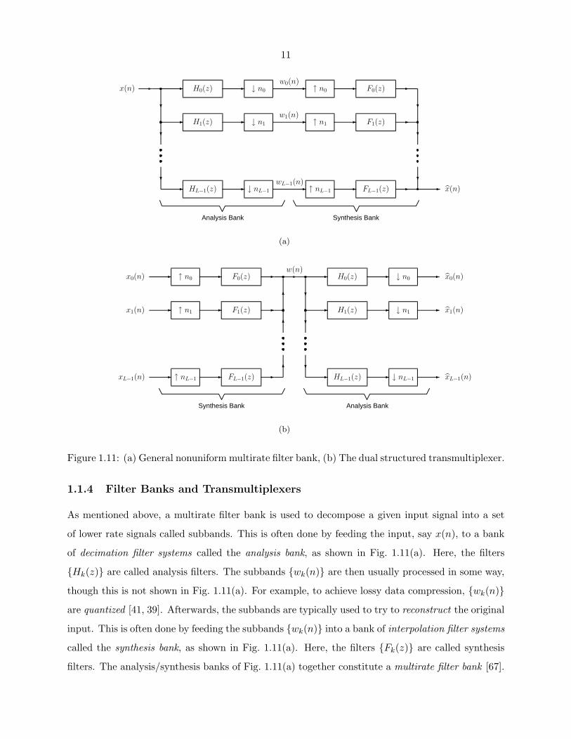
1.1.4 Filter Banks and Transmultiplexers

As mentioned above, a multirate filter bank is used to decompose a given input signal into a set

of lower rate signals called subbands. This is often done by feeding the input, say x(n), to a bank

of decimation filter systems called the analysis bank, as shown in Fig. 1.11(a). Here, the filters

{Hk(z)} are called analysis filters. The subbands {wk(n)} are then usually processed in some way,

though this is not shown in Fig. 1.11(a). For example, to achieve lossy data compression, {wk(n)}are quantized [41, 39]. Afterwards, the subbands are typically used to try to reconstruct the original

input. This is often done by feeding the subbands {wk(n)} into a bank of interpolation filter systems

called the synthesis bank, as shown in Fig. 1.11(a). Here, the filters {Fk(z)} are called synthesis

filters. The analysis/synthesis banks of Fig. 1.11(a) together constitute a multirate filter bank [67].

12

By reversing the roles of the analysis and synthesis banks, we obtain the dual to the multirate

filter bank known as the transmultiplexer [67], as shown in Fig. 1.11(b). Whereas filter banks are

typically used for source coding applications such as data compression, transmultiplexers are often

used for channel coding applications in digital communications. The transmultiplexer model of

Fig. 1.11(b) may represent, for example, a digital communications system in which we have L users

{xk(n)} who wish to transmit data over a common path. After passing through the channel, the

data from each user must be isolated and recovered, yielding the received signals {xk(n)}.The systems of Fig. 1.11 are given special names according to the overall rate of the subband

signals, which depend on the nature of the decimator/expander values {nk} used. Note that the

overall rate of the subband signals is simply

(L−1∑k=0

1nk

)times the input rate. If we have

L−1∑k=0

1nk

= 1

then the filter bank is said to be maximally decimated, whereas the transmultiplexer will be said

to be minimally expanded. In this case, we may have neither a loss of information nor redundancy.

On the other hand, if we haveL−1∑k=0

1nk

< 1

then the filter bank will be said to be overdecimated, whereas the transmultiplexer will be said to

be underexpanded. In this case, the filter bank incurs a loss of information, whereas the transmul-

tiplexer system possesses redundancy. Finally, if we have

L−1∑k=0

1nk

> 1

then the filter bank will be said to be underdecimated, whereas the transmultiplexer will be said to

be overexpanded. In this case, the filter bank system has redundancy, whereas the transmultiplexer

incurs a loss of information.

If x(n) = x(n) for all x(n) for the filter bank system or xk(n) = xk(n) for all k and for all {xk(n)}for the transmultiplexer system, then each system is said to possess the perfect reconstruction (PR)

property1 [67]. If all of the decimator/expander values {nk} are equal, the systems of Fig. 1.11 are

said to be uniform. For arbitrary values of {nk}, these systems are said to be nonuniform.1A more general definition of the PR condition [67] is a distortionless reconstruction in which we have x(n) =

cx(n − D) for the filter bank system or xk(n) = ckxk(n − Dk) for the transmultiplexer system. Here, c and {ck}represent scale factors, whereas D and {Dk} denote delay values. Since scale factors and delays can often easily beabsorbed into the analysis/synthesis filters, for the remainder of the thesis, we will only be concerned with the stricterPR property defined above.

13

� �

�

�

↓ M

↓ M

↓ M

�z

�z

�z

�

�

�

H(z)

�

�

�

x(n)

x(n)

� w0(n)

w1(n)

wL−1(n)

�

�

�

F(z)

�

�

�

z−1

z−1

z−1

�↑ M

↑ M

↑ M

x(n)

x(n)

�

(a)

�

�

�

F(z)

�

�

�

x0(n)

x1(n)

xL−1(n)

�

�

�

H(z)

x0(n)

x1(n)

xL−1(n)

(b)

Figure 1.12: Polyphase representations of (a) uniform filter bank, (b) uniform transmultiplexer.

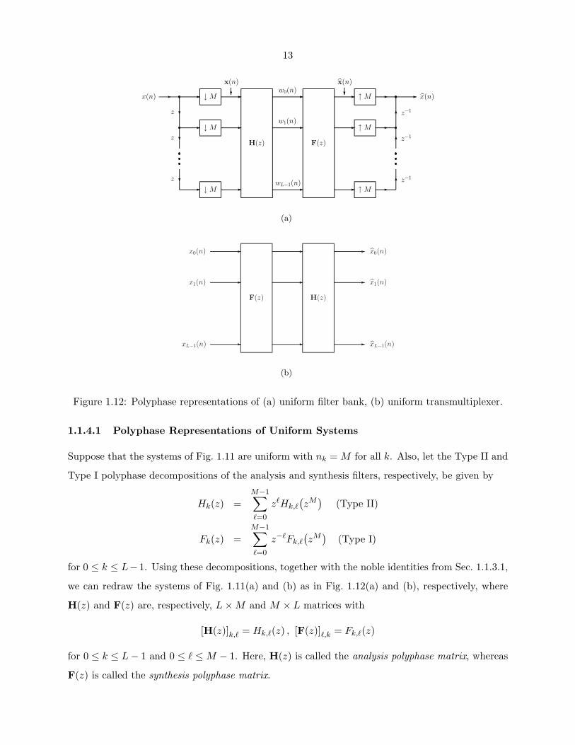
1.1.4.1 Polyphase Representations of Uniform Systems

Suppose that the systems of Fig. 1.11 are uniform with nk = M for all k. Also, let the Type II and

Type I polyphase decompositions of the analysis and synthesis filters, respectively, be given by

Hk(z) =M−1∑�=0

z�Hk,�

(zM

)(Type II)

Fk(z) =M−1∑�=0

z−�Fk,�

(zM

)(Type I)

for 0 ≤ k ≤ L−1. Using these decompositions, together with the noble identities from Sec. 1.1.3.1,

we can redraw the systems of Fig. 1.11(a) and (b) as in Fig. 1.12(a) and (b), respectively, where

H(z) and F(z) are, respectively, L × M and M × L matrices with

[H(z)]k,� = Hk,�(z) , [F(z)]�,k = Fk,�(z)

for 0 ≤ k ≤ L − 1 and 0 ≤ � ≤ M − 1. Here, H(z) is called the analysis polyphase matrix, whereas

F(z) is called the synthesis polyphase matrix.

14

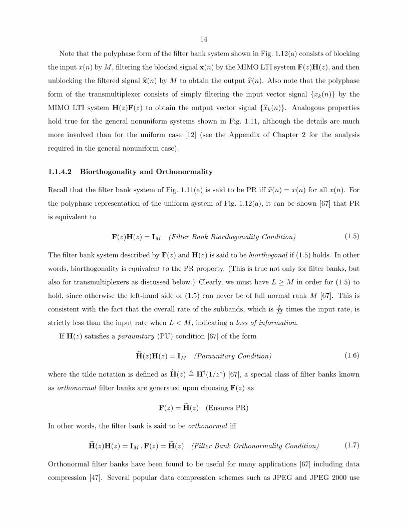
Note that the polyphase form of the filter bank system shown in Fig. 1.12(a) consists of blocking

the input x(n) by M , filtering the blocked signal x(n) by the MIMO LTI system F(z)H(z), and then

unblocking the filtered signal x(n) by M to obtain the output x(n). Also note that the polyphase

form of the transmultiplexer consists of simply filtering the input vector signal {xk(n)} by the

MIMO LTI system H(z)F(z) to obtain the output vector signal {xk(n)}. Analogous properties

hold true for the general nonuniform systems shown in Fig. 1.11, although the details are much

more involved than for the uniform case [12] (see the Appendix of Chapter 2 for the analysis

required in the general nonuniform case).

1.1.4.2 Biorthogonality and Orthonormality

Recall that the filter bank system of Fig. 1.11(a) is said to be PR iff x(n) = x(n) for all x(n). For

the polyphase representation of the uniform system of Fig. 1.12(a), it can be shown [67] that PR

is equivalent to

F(z)H(z) = IM (Filter Bank Biorthogonality Condition) (1.5)

The filter bank system described by F(z) and H(z) is said to be biorthogonal if (1.5) holds. In other

words, biorthogonality is equivalent to the PR property. (This is true not only for filter banks, but

also for transmultiplexers as discussed below.) Clearly, we must have L ≥ M in order for (1.5) to

hold, since otherwise the left-hand side of (1.5) can never be of full normal rank M [67]. This is

consistent with the fact that the overall rate of the subbands, which is LM times the input rate, is

strictly less than the input rate when L < M , indicating a loss of information.

If H(z) satisfies a paraunitary (PU) condition [67] of the form

H(z)H(z) = IM (Paraunitary Condition) (1.6)

where the tilde notation is defined as H(z) � H†(1/z∗) [67], a special class of filter banks known

as orthonormal filter banks are generated upon choosing F(z) as

F(z) = H(z) (Ensures PR)

In other words, the filter bank is said to be orthonormal iff

H(z)H(z) = IM ,F(z) = H(z) (Filter Bank Orthonormality Condition) (1.7)

Orthonormal filter banks have been found to be useful for many applications [67] including data

compression [47]. Several popular data compression schemes such as JPEG and JPEG 2000 use

15

orthonormal filter banks to obtain good lossy data compression [41, 39]. Orthonormal filter banks

have several advantages which make them very attractive to use. For example, orthonormal filter

banks preserve the energy of the input signal in the subbands (i.e., the �2 norm of the subband

signals equals that of the input signal [67]), which may be useful if we wish to avoid overamplifying

or overattenuating the subbands. Also, orthonormal filter banks only require the design of either the

analysis or synthesis polyphase matrix, since the analysis/synthesis polyphase matrices are related

as F(z) = H(z). Finally, if the analysis filters {Hk(z)} or equivalently the analysis polyphase matrix

H(z) of an orthonormal filter bank are FIR, then the corresponding synthesis filters {Fk(z)} and

synthesis polyphase matrix F(z) are also necessarily FIR.

Biorthogonality and orthonormality conditions also exist for the transmultiplexer system of

Fig. 1.11(b). In particular, for the uniform system of Fig. 1.12(b), the biorthogonality condition

becomes

H(z)F(z) = IL (Transmulitplexer Biorthogonality Condition) (1.8)

Clearly, we must have L ≤ M here in order for (1.8) to hold, since otherwise the left-hand side

of (1.8) can never be of full normal rank L [67]. Analogous with the filter bank system, this is

consistent with the fact that when L > M , we have a loss of information. Similar to (1.7), the

orthonormality condition for the transmultiplexer system of Fig. 1.12(b) is given by

F(z)F(z) = IL ,H(z) = F(z) (Transmultiplexer Orthonormality Condition) (1.9)

It should be noted that biorthogonality and orthonormality conditions analogous to those given

in (1.5), (1.8), (1.7), and (1.9) exist for the general nonuniform systems shown in Fig. 1.11. The

interested reader is referred to [67, 45, 12] for more details.

1.2 Signal-Adapted Filter Banks

Any filter bank whose filters somehow depend on any knowledge of the input statistics is called

a signal-adapted filter bank. A typical model for a signal-adapted filter bank that will be used

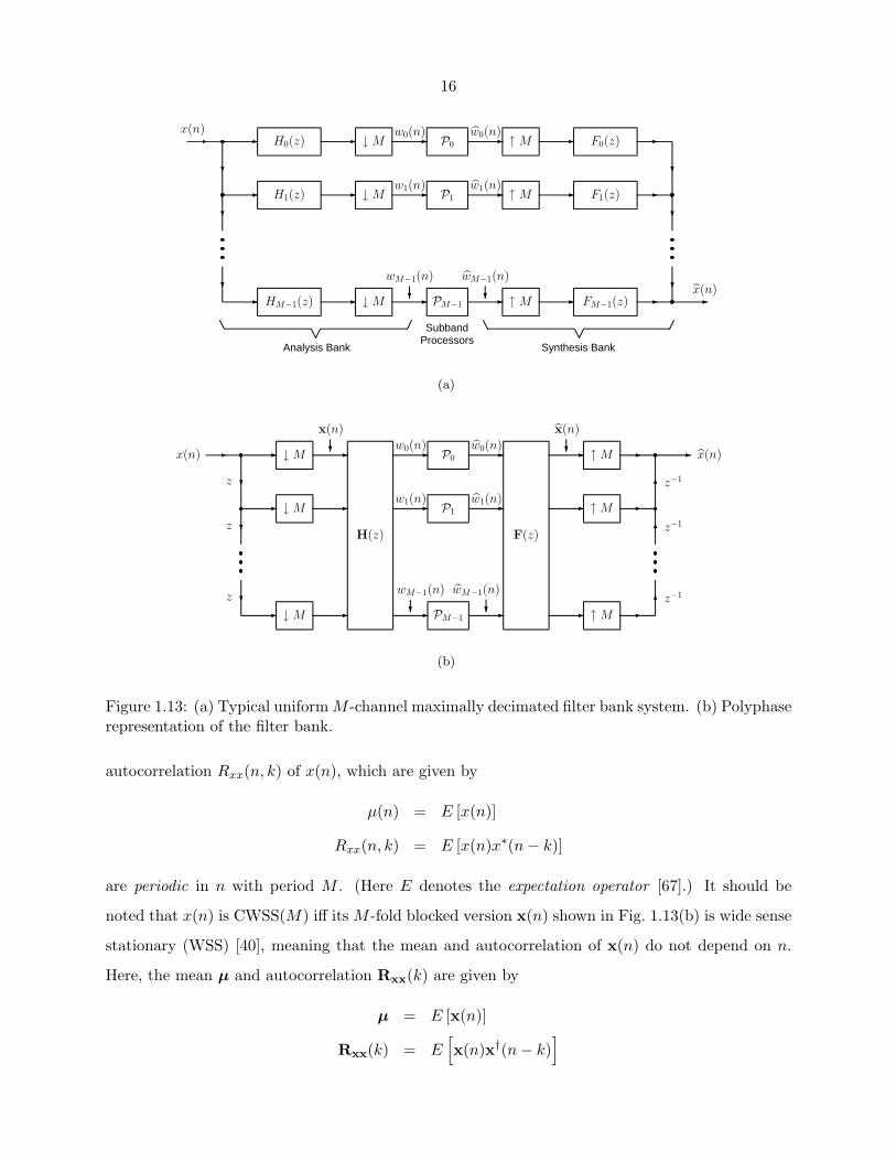
throughout the thesis is the uniform M -channel maximally decimated filter bank shown in Fig.

1.13(a). The M -fold polyphase representation of this filter bank is shown in Fig. 1.13(b). Here,

the subband processors {Pk} may be nonlinear systems such as scalar quantizers or thresholding

devices or linear filters for denoising.

Throughout the thesis, we will assume that the input signal x(n) is a cyclo wide sense station-

ary process with period M (abbreviated CWSS(M)) [40]. This means that the mean µ(n) and

16

� � H0(z)

�

� H1(z)

�

�

� HM−1(z)

�

�

�

↓ M

↓ M

↓ M

�

�

�

Analysis Bank

x(n) w0(n)

w1(n)

wM−1(n)

�

P0

P1

PM−1

�

�

�

↑ M

↑ M

↑ M

�

�

�

F0(z)

F1(z)

FM−1(z)

�

�

�

�

�

�

�

Synthesis Bank

x(n)

w0(n)

w1(n)

wM−1(n)

�

SubbandProcessors

(a)

� �

�

�

↓ M

↓ M

↓ M

�z

�z

�z

�

�

�

H(z)

�

�

�

x(n)w0(n)

w1(n)

wM−1(n)

�

x(n)

� P0

P1

PM−1

�

�

�

F(z)

�

�

�

�

�

�

z−1

z−1

z−1

�↑ M

↑ M

↑ M

x(n)w0(n)

w1(n)

wM−1(n)

�

x(n)

�

(b)

Figure 1.13: (a) Typical uniform M -channel maximally decimated filter bank system. (b) Polyphaserepresentation of the filter bank.

autocorrelation Rxx(n, k) of x(n), which are given by

µ(n) = E [x(n)]

Rxx(n, k) = E [x(n)x∗(n − k)]

are periodic in n with period M . (Here E denotes the expectation operator [67].) It should be

noted that x(n) is CWSS(M) iff its M -fold blocked version x(n) shown in Fig. 1.13(b) is wide sense

stationary (WSS) [40], meaning that the mean and autocorrelation of x(n) do not depend on n.

Here, the mean µ and autocorrelation Rxx(k) are given by

µ = E [x(n)]

Rxx(k) = E[x(n)x†(n − k)

]

17

For the remainder of the thesis, we will assume that x(n) and hence x(n) are zero mean. Also, we

will assume that we only have knowledge of the second order statistics of x(n) (namely, Rxx(k)),

in addition to the given zero mean assumption on x(n). An equivalent representation of the

autocorrelation Rxx(k) that will be commonly used is the power spectral density (psd) Sxx(z),

which is simply the z-transform of Rxx(k).

1.2.1 Principal Component Filter Banks

Focusing on Fig. 1.13(b), often times, for simplicity of design as well as for other reasons, we will

restrict our attention to orthonormal or PU filter banks in which we have2

F(z)F(z) = I , H(z) = F(z) (1.10)

Recently, it has been shown that a special type of PU filter bank matched to the input statistics

Sxx(z) known as the principal component filter bank (PCFB) [62] is simultaneously optimal for

a variety of objective functions [1]. Among these objectives are included several important data

compression objectives such as mean-squared error under the presence of quantization noise [28]

(for any bit allocation) and coding gain [68, 69] (with optimal bit allocation). By definition, a

PCFB for an input psd Sxx(z) and for a class C of filter banks, if it exists, is one whose subband

variance vector

σ �[

σ2w0

σ2w1

· · · σ2wM−1

]T(1.11)

majorizes [22] any other subband variance vector arising from any other filter bank in C. (Recall

that a vector a �[

a0 a1 · · · aP−1

]T

with a0 ≥ a1 ≥ · · · ≥ aP−1 ≥ 0 is said to majorize [22]

a vector b �[

b0 b1 · · · bP−1

]T

with b0 ≥ b1 ≥ · · · ≥ bP−1 ≥ 0 iff we have

p∑k=0

ak ≥p∑

k=0

bk ∀ 0 ≤ p ≤ P − 2 ,P−1∑k=0

ak =P−1∑k=0

bk .)

In addition to being optimal for coding gain and mean-squared error in the presence of quantization

noise, the PCFB has also been shown to be optimal for any concave objective function of σ [1].2It should be noted that (1.10) is equivalent to the orthonormality condition given in (1.7) since the filter bank

is maximally decimated. Here, we have opted for the form given in (1.10), in which we focus on the design of thesynthesis bank, as it will be more natural when we constrain the synthesis filters to be causal FIR. These filters arecausal FIR iff F(z) is as well. This is not however true for the analysis filters and H(z) on account of the advancechain present in the blocking system.

18

1.2.1.1 Classes for Which PCFBs Are Known to Exist

Though PCFBs exhibit many optimal characteristics, they are only known to exist for special

classes of filter banks [1]. One notable exception to this is for the special case where M = 2, in

which case a PCFB always exists for any class of PU filter banks [1]. For general M , however,

PCFBs are known to exist only for two special classes. If C is the class of all transform coders

Ct, in which F(z) is a constant unitary matrix T, then the PCFB exists and is the Karhunen-

Loeve transform (KLT) for the input process x(n) (i.e., T diagonalizes the autocorrelation matrix

Rxx(0)) [23, 1]. Furthermore, if C is the class of all (unconstrained order) PU filter banks Cu, then

the PCFB exists and is the pointwise in frequency KLT for x(n) [68, 1, 69]. By this, we mean

that F(ejω) diagonalizes (i.e., totally decorrelates) Sxx(ejω) for every ω such that the frequency

dependent eigenvalues are always arranged in decreasing order, which is a property called spectral

majorization [68]. For many practical cases of inputs (for example, if the scalar input signal x(n)

is itself WSS), the corresponding analysis and synthesis filters are ideal bandpass filters called

compaction filters [68, 66, 65] (see Chapter 2 for more on compaction filters). As such, they are

unrealizable in practice. However, they serve to compute an upper bound on the performance that

we can expect from a PU filter bank.

1.2.1.2 Difficulties with the Class of FIR PU Systems

The problem with the class of FIR PU filter banks in which F(z) has finite memory (or more

appropriately finite McMillan degree3) is that it is believed that a PCFB doesn’t exist [27, 1, 24],

although this has not yet been formally proven. Instead, for this class, F(z) is typically chosen

to optimize a specific objective for a given input psd, such as coding gain [11, 8, 35, 79], rate-

distortion [36], or a multiresolution energy compaction criterion [37]. All such methods require the

numerical optimization of nonlinear and nonconvex objective functions which offer little insight

into the behavior of the solutions as the filter order (i.e., the memory of F(z)) increases.

Another common approach is to calculate an optimal FIR compaction filter [64, 59] (for the

first filter F0(z)) and then obtain the rest of the filters via an appropriate filter bank completion for

a multiresolution criterion [37, 49]. Though elegant in the sense that the filter bank design problem

is tantamount to calculating an FIR compaction filter followed by an appropriate KLT, it suffers

from the ambiguity caused by the nonuniqueness of the FIR compaction filter. Different compaction3The McMillan degree of a causal MIMO system is defined as the minimum number of delay elements required to

implement the system [67].

19

filter spectral factors lead to different filter banks which in turn yield different performances (as

is shown in Chapter 3). As such, all such spectral factors need to be tested for their performance

[49], which is exponentially computationally complex with respect to the compaction filter order.

Finally, none of the above-mentioned methods for the design of FIR PU signal-adapted filter

banks in the literature have been shown to tend toward the infinite-order PCFB solution as the

FIR degree or order increases. Intuition tells us that as the order increases, any FIR PU filter bank

designed to optimize any one objective for which the PCFB is optimal will tend to behave more

and more like the infinite-order PCFB, though this has not previously been shown in the literature.

One of the major contributions of this thesis is to show this behavior and to bridge the gap between

the zeroth-order KLT and infinite-order PCFB (see Chapters 3 and 4).

1.3 The FIR PU Interpolation Problem

In certain applications, it may be necessary for an FIR PU system, say F(ejω), to take on a

prescribed set of values over a prescribed set of frequencies. For example, suppose that for the

frequencies ω0, ω1, . . . , ωL−1, we require

F(ejωk) = Uk ∀ 0 ≤ k ≤ L − 1 (1.12)

Evidently, the matrices {Uk} must be unitary in light of the PU assumption on F(ejω). The problem

of finding an FIR PU system of a certain McMillan degree which satisfies (1.12) is known as the

FIR PU interpolation problem [71].

In the traditional FIR interpolation problem, in which the only restriction made on the inter-

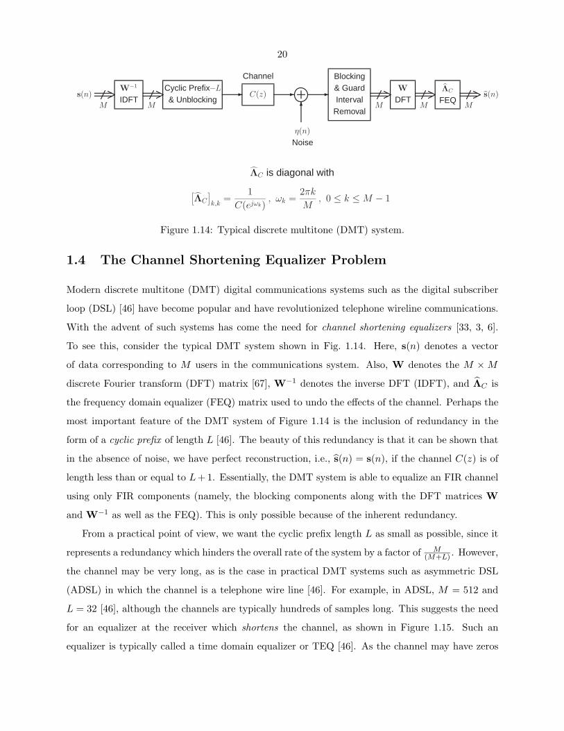
polant is the FIR constraint, we can always find an interpolant of length at most equal to the

number of interpolation conditions by using the Lagrange interpolation formula [22]. However, for

the FIR PU interpolation problem of (1.12), in general, it is not known whether there even exists

an interpolant of finite degree which will satisfy all L conditions from (1.12). For the special case in

which F(ejω) is scalar, it is known that in general, only one condition from (1.12) can be satisfied

(since in this case, F(z) is necessarily a pure delay [71]).

Though there is no known solution to the FIR PU interpolation problem, using the optimization

algorithm presented in Chapter 4, we can find an approximant to an interpolant. For cases where an

interpolant of a certain degree is known to exist, this algorithm can be used to find the interpolant.

One of the contributions of the thesis here is thus a numerical approach to solve a theoretically

intractable problem.

20

M

W−1

IDFTM

Cyclic Prefix−L

& Unblocking� C(z) �

�

Blocking& GuardInterval

RemovalM

W

DFTM

ΛC

FEQM

s(n) s(n)

Channel

η(n)

Noise

ΛC is diagonal with

[ΛC

]k,k

=1

C(ejωk), ωk =

2πk

M, 0 ≤ k ≤ M − 1

Figure 1.14: Typical discrete multitone (DMT) system.

1.4 The Channel Shortening Equalizer Problem

Modern discrete multitone (DMT) digital communications systems such as the digital subscriber

loop (DSL) [46] have become popular and have revolutionized telephone wireline communications.

With the advent of such systems has come the need for channel shortening equalizers [33, 3, 6].

To see this, consider the typical DMT system shown in Fig. 1.14. Here, s(n) denotes a vector

of data corresponding to M users in the communications system. Also, W denotes the M × M

discrete Fourier transform (DFT) matrix [67], W−1 denotes the inverse DFT (IDFT), and ΛC is

the frequency domain equalizer (FEQ) matrix used to undo the effects of the channel. Perhaps the

most important feature of the DMT system of Figure 1.14 is the inclusion of redundancy in the

form of a cyclic prefix of length L [46]. The beauty of this redundancy is that it can be shown that

in the absence of noise, we have perfect reconstruction, i.e., s(n) = s(n), if the channel C(z) is of

length less than or equal to L + 1. Essentially, the DMT system is able to equalize an FIR channel

using only FIR components (namely, the blocking components along with the DFT matrices W

and W−1 as well as the FEQ). This is only possible because of the inherent redundancy.

From a practical point of view, we want the cyclic prefix length L as small as possible, since it

represents a redundancy which hinders the overall rate of the system by a factor of M(M+L) . However,

the channel may be very long, as is the case in practical DMT systems such as asymmetric DSL

(ADSL) in which the channel is a telephone wire line [46]. For example, in ADSL, M = 512 and

L = 32 [46], although the channels are typically hundreds of samples long. This suggests the need

for an equalizer at the receiver which shortens the channel, as shown in Figure 1.15. Such an

equalizer is typically called a time domain equalizer or TEQ [46]. As the channel may have zeros

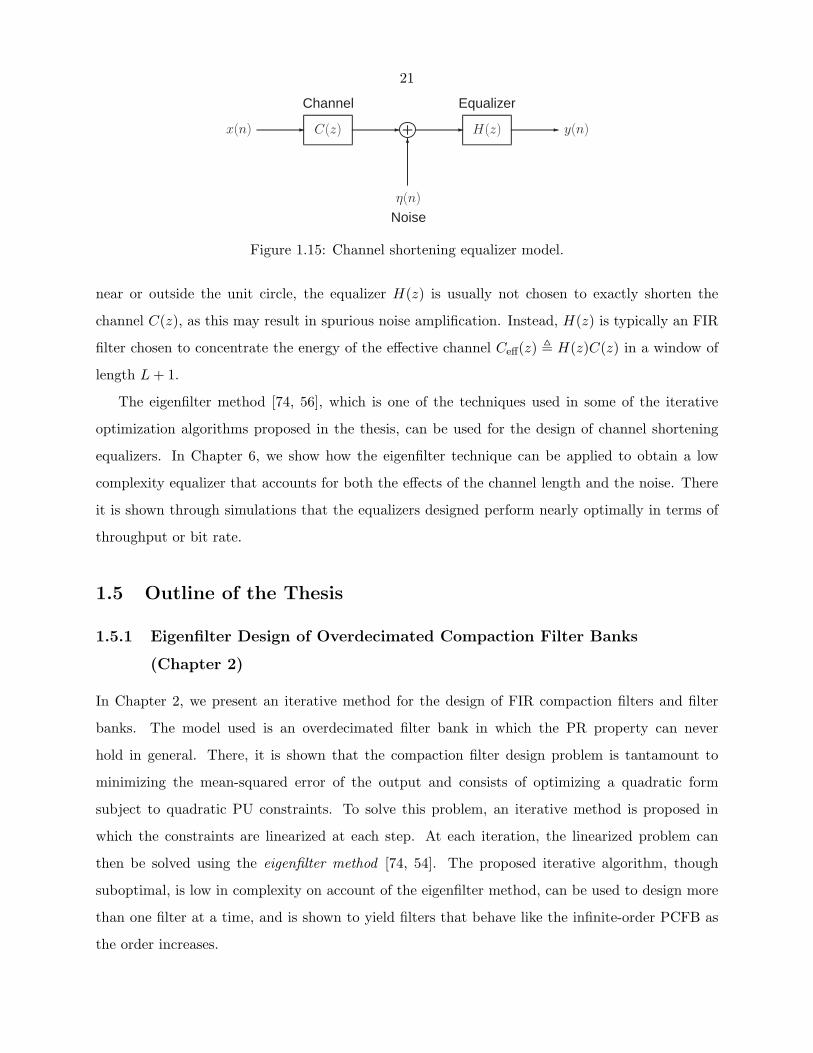
21

� C(z) � � H(z) �

x(n)

Channel Equalizer

y(n)

η(n)

Noise

Figure 1.15: Channel shortening equalizer model.

near or outside the unit circle, the equalizer H(z) is usually not chosen to exactly shorten the

channel C(z), as this may result in spurious noise amplification. Instead, H(z) is typically an FIR

filter chosen to concentrate the energy of the effective channel Ceff(z) � H(z)C(z) in a window of

length L + 1.

The eigenfilter method [74, 56], which is one of the techniques used in some of the iterative

optimization algorithms proposed in the thesis, can be used for the design of channel shortening

equalizers. In Chapter 6, we show how the eigenfilter technique can be applied to obtain a low

complexity equalizer that accounts for both the effects of the channel length and the noise. There

it is shown through simulations that the equalizers designed perform nearly optimally in terms of

throughput or bit rate.

1.5 Outline of the Thesis

1.5.1 Eigenfilter Design of Overdecimated Compaction Filter Banks

(Chapter 2)

In Chapter 2, we present an iterative method for the design of FIR compaction filters and filter

banks. The model used is an overdecimated filter bank in which the PR property can never

hold in general. There, it is shown that the compaction filter design problem is tantamount to

minimizing the mean-squared error of the output and consists of optimizing a quadratic form

subject to quadratic PU constraints. To solve this problem, an iterative method is proposed in

which the constraints are linearized at each step. At each iteration, the linearized problem can

then be solved using the eigenfilter method [74, 54]. The proposed iterative algorithm, though

suboptimal, is low in complexity on account of the eigenfilter method, can be used to design more

than one filter at a time, and is shown to yield filters that behave like the infinite-order PCFB as

the order increases.

22

1.5.2 Multiresolution Optimal FIR PU Filter Banks (Chapter 3)

Though very low in complexity, the iterative eigenfilter method for compaction filter design suffers

from the drawbacks that the quadratic PU constraints may not be satisfied and also that the

performance in terms of compaction gain tends to saturate well below that of the infinite-order

PCFB as the order increases. To alleviate this problem, in Chapter 3, a different iterative algorithm

is proposed for the design of compaction filters. Using a complete parameterization of all FIR

PU systems in terms of degree-one Householder building blocks [75, 67], an iterative algorithm

for designing an FIR compaction filter is presented in which the objective is to approximate the

infinite-order PCFB compaction filter in the least-squares sense. This ensures that the desired

PU constraint is always in effect. At each iteration, one set of parameters in the Householder-like

characterization of the compaction filter is globally optimized assuming all other parameters are

fixed. As such, the algorithm is greedy and the mean-squared error at every iteration is guaranteed

to be monotonic nonincreasing per iteration.

Since the phase of the infinite-order PCFB compaction filter is arbitrary (see Chapters 2 and

4), a modification is proposed in which the phase of the FIR compaction filter is fed back to the

desired infinite-order compaction filter response. In essence, this modification, which we call the

phase feedback modification, allows the algorithm to find an easier phase to approximate with an

FIR solution. With this modification in effect, it is shown that the algorithm not only still remains

greedy, but also results in better FIR compaction filters in terms of compaction gain. Simulation

results show a monotonic increase in compaction gain as a function of filter order that comes very

close to the infinite-order compaction filter bound.

To obtain the rest of the filters of a maximally decimated signal-adapted orthonormal filter

bank, a multiresolution optimality criterion [62, 37] is used. With this criterion, the entire filter

bank is elegantly designed using only an FIR compaction filter followed by a simple KLT. Though

elegant, this criterion is shown to suffer from the inherent nonuniqueness of the FIR compaction

filter in terms of its different spectral factors. Different spectral factors lead to different filter banks

which in turn yield different performances. By choosing the spectral factor which yields the largest

coding gain, it is shown that the FIR filter banks designed perform more and more like the infinite-

order PCFB in terms of several objectives as the FIR order increases. This serves to bridge the gap

between the zeroth-order KLT and infinite-order PCFB.

23

1.5.3 Direct FIR PU Approximation of the PCFB (Chapter 4)

Due to the inherent nonuniqueness of an FIR compaction filter in terms of its spectral factors,

designing signal-adapted filter banks using the multiresolution criterion used in Chapter 3 becomes

computationally intractable as the filter order increases. This is because the number of spectral

factors and hence filter banks whose performance must be tested grows exponentially with order.

To avoid this problem, in Chapter 4, the iterative algorithm of Chapter 3 is generalized to obtain all

of the synthesis filters at the same time. In particular, a method is proposed for solving the general

weighted least-squares approximation problem for the matrix case using an FIR PU approximant.

Using the above-mentioned Householder-like factorization of such systems, an iterative algorithm is

proposed in which a set of parameters is globally optimized at each iteration assuming all others are

fixed. As such, the algorithm is greedy in the same way in which the one from Chapter 3 is as well.

To design an FIR PU signal-adapted filter bank, the proposed algorithm is used to approximate

the synthesis polyphase matrix of an infinite-order PCFB. With this method, all of the filters are

obtained at the same time with only a marginal increase in complexity over the method of Chapter

3. As the infinite-order PCFB synthesis polyphase matrix exhibits a phase-type ambiguity (which

we formally define in Chapter 4), a generalization of the phase feedback modification from Chapter 3

to the matrix case is proposed. With this modification in effect, the algorithm not only still remains

greedy but also yields a better magnitude-type fit for the synthesis filters. As all of the filters are

found together, this eliminates the need to complete the filter bank using an FIR compaction

filter as well as the problems caused by the nonuniqueness of this filter. Simulation results show

that the FIR PU signal-adapted filter banks designed using this method behave more and more

like the infinite-order PCFB in terms of numerous objectives as the order increases. As with the

method proposed in Chapter 3, this serves to bridge the gap between the zeroth-order KLT and the

infinite-order PCFB. However, this method avoids the need to check the performance of different

compaction filter spectral factors, which is exponentially computationally complex with filter order.

In addition to being useful for the design of signal-adapted filter banks, the proposed algorithm

can also be used for the FIR PU interpolation problem through proper choice of the weight function.

Though this problem is still open, the proposed algorithm can always be used to find an approximant

to a desired interpolant. For cases where an interpolant is known to exist, the proposed algorithm

can be used to find this interpolant, as simulations show.

24

1.5.4 Coding Gain Optimal FIR Filter Banks (Chapter 5)

In Chapter 5, we consider the optimal design of a signal-adapted filter bank in which the filters are

FIR but otherwise unconstrained. The model used is a uniform filter bank with a variable number of

channels with scalar quantizers in the subbands and the objective is to minimize the mean-squared

error observed at the filter bank output. This is equivalent to maximizing the coding gain of the

system. Assuming that the analysis (synthesis) bank is fixed, globally optimizing the corresponding

synthesis (analysis) bank is very simple and can be done using the principle of completing the square

[22], as is shown. This leads to an iterative greedy algorithm in which the analysis and synthesis

banks are alternately optimized. Simulation results verify the greediness of the algorithm and

exhibit its usefulness. When we ignore the effects due to quantization, the algorithm can be used

to design overdecimated filter banks for optimal reconstruction. In many cases, the filters designed

compact the energy of the input, much like the compaction filters of an infinite-order PCFB. Upon

accounting for the effects of quantization, it is shown that the quantization systems designed come

close to the information theoretic rate-distortion bound [10, 7] and coding gain bound [25]. As the

filter orders increase, the quantized filter banks designed come closer to these bounds, in line with

intuition. This phenomenon has previously not been shown in the literature.

1.5.5 Eigenfilter Channel Shortening Equalizer for DMT Systems (Chapter 6)

Chapter 6 differs in theme from the previous chapters in the sense that it is concerned with the

design of channel shortening equalizers for DMT systems. There, it is shown that the eigenfilter

method used in Chapter 2 can be used for this problem. In particular, we show how the eigenfilter

method can be used for the design of a fractionally spaced equalizer (FSE) for channel shortening

which jointly accounts for the effects due to the channel length as well as noise. One advantage

of this method is that it is lower in complexity than other commonly used methods. As opposed

to other similar methods which require a different Cholesky decomposition [22] of a certain matrix

for every delay parameter chosen, the proposed method only requires one. Despite a significant

decrease in complexity, it is shown that there is only a minimal loss in the observed bit rate or

throughput. Simulation results for various practical channels encountered in a DSL environment

show that the proposed method performs nearly optimally in terms of bit rate.

25

1.6 Notations

The notation used in the thesis closely parallels that used in [67]. In particular, the subscripts (∗),(T), and

(†) denote, respectively, the conjugate, transpose, and conjugate transpose of a general

matrix quantity. The real and imaginary parts of a complex number c will be denoted by Re[c]

and Im[c], respectively. Typically, boldface letters are used for matrices and vectors. The (k, �)-th

element of a matrix P will be denoted by [P]k,�. The notation diag (a0, a1, . . . , aM−1) is used to

denote an M × M diagonal matrix whose diagonal elements are the values a0, a1, . . . , aM−1 (i.e.,

if Λ = diag (a0, a1, . . . , aM−1), then [Λ]k,k = ak). Here, Tr [A] will be used to denote the trace

of a matrix A, which is the sum of its diagonal elements. Also, we will use ||A||F to denote the

Frobenius norm of any matrix A, which is defined as ||A||F �√

Tr [A†A] [22].

Lowercase letters are commonly used for discrete-time sequences, whereas uppercase letters are

often used for Fourier and z-transforms. Together with Fig. 1.3(a) and 1.4(a), (1.1) establishes

the notation that will be used for expanders and decimators. For any matrix system H(z), its

paraconjugate H†(1/z∗) [67] will be denoted by H(z).

Finally, in line with standard notation used in statistical signal processing [48], E [·] will be

used to denote the expectation operator.

26

Chapter 2

Eigenfilter Design of OverdecimatedCompaction Filter Banks

In this chapter, a method is proposed for the design of a uniform overdecimated FIR PU filter

bank optimized for energy compaction. If no FIR constraint is imposed, then the corresponding

optimal filters are unconstrained order PCFB filters. For many practical cases of inputs, these

filters are ideal bandpass filters called compaction filters, as is shown here. As such, these filters

are necessarily of infinite-order.

When an FIR constraint is imposed on the energy compaction objective, the problem becomes

tantamount to maximizing a quadratic form subject to quadratic (and often singular) constraints,

as we show here. The method proposed to solve this problem consists of iteratively linearizing the

singular quadratic constraints. At each iteration, the eigenfilter approach [74, 56] can be used to

solve this problem, as is shown. Simulations provided show that the filters designed behave like

those of the infinite-order PCFB as the order increases.

Finally, we expand on some of the optimality properties of PU overdecimated filter banks in

general. This is shown not only for the uniform overdecimated filter bank considered here, but also

for a more general rational nonuniform overdecimated synthesis bank signal approximation model.

It turns out that for this model, the optimal driving signals are generated by a corresponding

overdecimated analysis bank as we show here. If the synthesis bank satisfies a PU condition similar

to (1.6), then the corresponding optimal analysis bank is just the paraconjugate of the synthesis

bank, yielding an orthonormal overdecimated system.

The content of this chapter is mainly drawn from [54, 49] and portions of it have been presented

at [57].

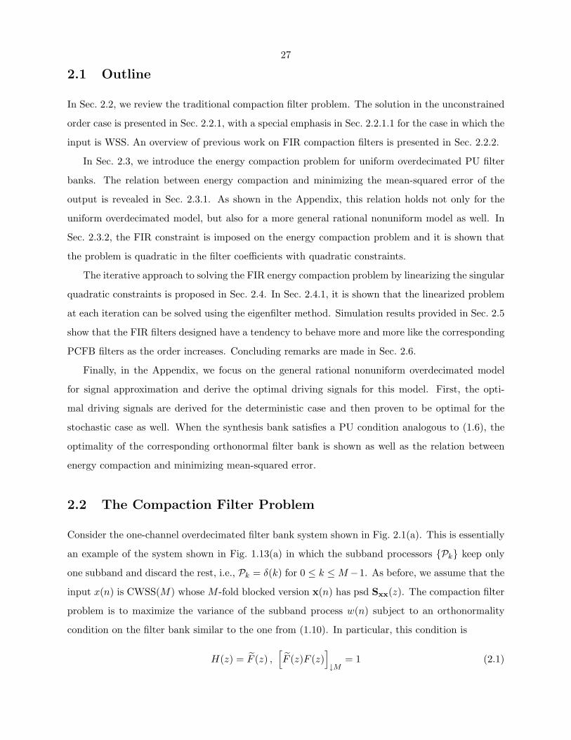
27

2.1 Outline

In Sec. 2.2, we review the traditional compaction filter problem. The solution in the unconstrained

order case is presented in Sec. 2.2.1, with a special emphasis in Sec. 2.2.1.1 for the case in which the

input is WSS. An overview of previous work on FIR compaction filters is presented in Sec. 2.2.2.

In Sec. 2.3, we introduce the energy compaction problem for uniform overdecimated PU filter

banks. The relation between energy compaction and minimizing the mean-squared error of the

output is revealed in Sec. 2.3.1. As shown in the Appendix, this relation holds not only for the

uniform overdecimated model, but also for a more general rational nonuniform model as well. In

Sec. 2.3.2, the FIR constraint is imposed on the energy compaction problem and it is shown that

the problem is quadratic in the filter coefficients with quadratic constraints.

The iterative approach to solving the FIR energy compaction problem by linearizing the singular

quadratic constraints is proposed in Sec. 2.4. In Sec. 2.4.1, it is shown that the linearized problem

at each iteration can be solved using the eigenfilter method. Simulation results provided in Sec. 2.5

show that the FIR filters designed have a tendency to behave more and more like the corresponding

PCFB filters as the order increases. Concluding remarks are made in Sec. 2.6.

Finally, in the Appendix, we focus on the general rational nonuniform overdecimated model

for signal approximation and derive the optimal driving signals for this model. First, the opti-

mal driving signals are derived for the deterministic case and then proven to be optimal for the

stochastic case as well. When the synthesis bank satisfies a PU condition analogous to (1.6), the

optimality of the corresponding orthonormal filter bank is shown as well as the relation between

energy compaction and minimizing mean-squared error.

2.2 The Compaction Filter Problem

Consider the one-channel overdecimated filter bank system shown in Fig. 2.1(a). This is essentially

an example of the system shown in Fig. 1.13(a) in which the subband processors {Pk} keep only

one subband and discard the rest, i.e., Pk = δ(k) for 0 ≤ k ≤ M −1. As before, we assume that the

input x(n) is CWSS(M) whose M -fold blocked version x(n) has psd Sxx(z). The compaction filter

problem is to maximize the variance of the subband process w(n) subject to an orthonormality

condition on the filter bank similar to the one from (1.10). In particular, this condition is

H(z) = F (z) ,[F (z)F (z)

]↓M

= 1 (2.1)

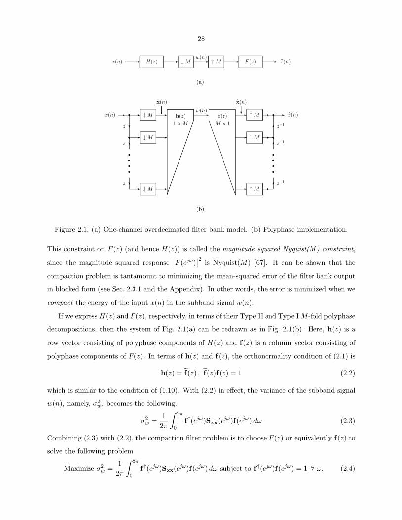
28

� H(z) � ↓ M �x(n) F (z) �↑ M � x(n)w(n)

(a)

� �

�

�

↑ M

↑ M

↑ M

�

�

�

��

�

�

↓ M

↓ M

↓ M

�

�

�

�

�

�

�x(n) x(n)

z

z

z z−1

z−1

z−1

x(n)

�

x(n)

�w(n)f(z)

M × 1

h(z)

1 × M

(b)

Figure 2.1: (a) One-channel overdecimated filter bank model. (b) Polyphase implementation.

This constraint on F (z) (and hence H(z)) is called the magnitude squared Nyquist(M) constraint,

since the magnitude squared response∣∣F (ejω)

∣∣2 is Nyquist(M) [67]. It can be shown that the

compaction problem is tantamount to minimizing the mean-squared error of the filter bank output

in blocked form (see Sec. 2.3.1 and the Appendix). In other words, the error is minimized when we

compact the energy of the input x(n) in the subband signal w(n).

If we express H(z) and F (z), respectively, in terms of their Type II and Type I M -fold polyphase

decompositions, then the system of Fig. 2.1(a) can be redrawn as in Fig. 2.1(b). Here, h(z) is a

row vector consisting of polyphase components of H(z) and f(z) is a column vector consisting of

polyphase components of F (z). In terms of h(z) and f(z), the orthonormality condition of (2.1) is

h(z) = f(z) , f(z)f(z) = 1 (2.2)

which is similar to the condition of (1.10). With (2.2) in effect, the variance of the subband signal

w(n), namely, σ2w, becomes the following.

σ2w =

12π

∫ 2π

0f †(ejω)Sxx(ejω)f(ejω) dω (2.3)

Combining (2.3) with (2.2), the compaction filter problem is to choose F (z) or equivalently f(z) to

solve the following problem.

Maximize σ2w =

12π

∫ 2π

0f †(ejω)Sxx(ejω)f(ejω) dω subject to f †(ejω)f(ejω) = 1 ∀ ω. (2.4)

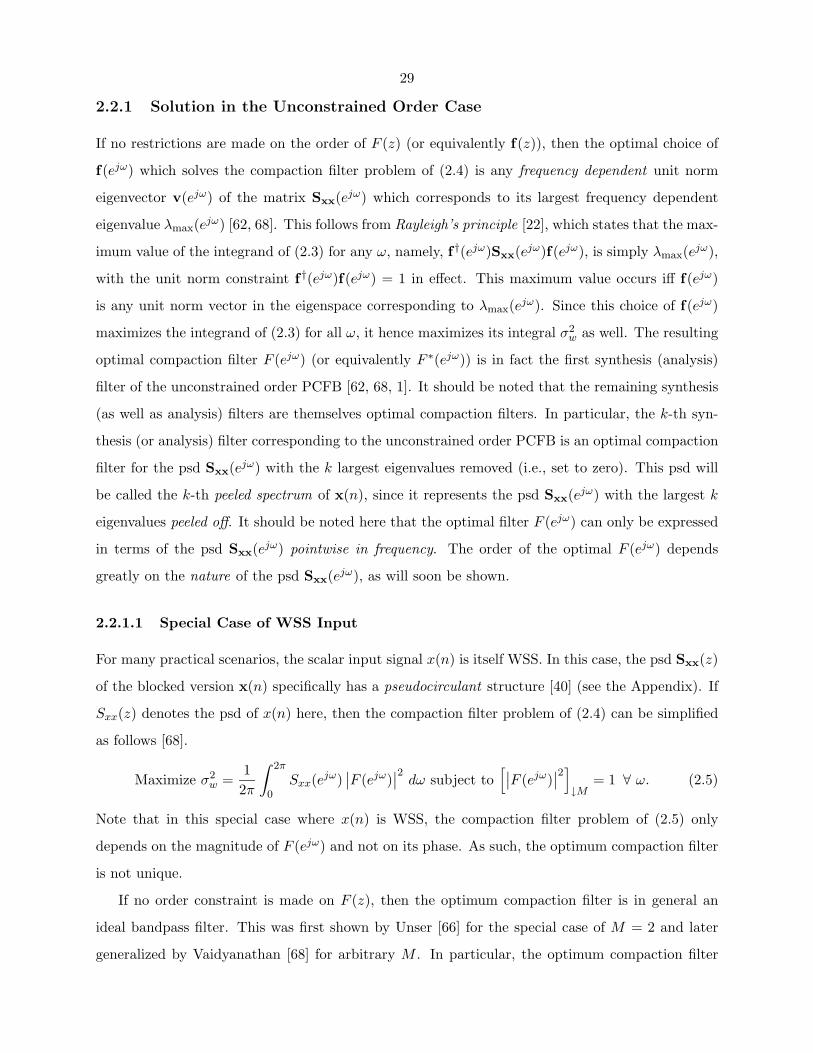
29

2.2.1 Solution in the Unconstrained Order Case

If no restrictions are made on the order of F (z) (or equivalently f(z)), then the optimal choice of

f(ejω) which solves the compaction filter problem of (2.4) is any frequency dependent unit norm

eigenvector v(ejω) of the matrix Sxx(ejω) which corresponds to its largest frequency dependent

eigenvalue λmax(ejω) [62, 68]. This follows from Rayleigh’s principle [22], which states that the max-

imum value of the integrand of (2.3) for any ω, namely, f †(ejω)Sxx(ejω)f(ejω), is simply λmax(ejω),

with the unit norm constraint f †(ejω)f(ejω) = 1 in effect. This maximum value occurs iff f(ejω)

is any unit norm vector in the eigenspace corresponding to λmax(ejω). Since this choice of f(ejω)

maximizes the integrand of (2.3) for all ω, it hence maximizes its integral σ2w as well. The resulting

optimal compaction filter F (ejω) (or equivalently F ∗(ejω)) is in fact the first synthesis (analysis)

filter of the unconstrained order PCFB [62, 68, 1]. It should be noted that the remaining synthesis

(as well as analysis) filters are themselves optimal compaction filters. In particular, the k-th syn-

thesis (or analysis) filter corresponding to the unconstrained order PCFB is an optimal compaction

filter for the psd Sxx(ejω) with the k largest eigenvalues removed (i.e., set to zero). This psd will

be called the k-th peeled spectrum of x(n), since it represents the psd Sxx(ejω) with the largest k

eigenvalues peeled off. It should be noted here that the optimal filter F (ejω) can only be expressed

in terms of the psd Sxx(ejω) pointwise in frequency. The order of the optimal F (ejω) depends

greatly on the nature of the psd Sxx(ejω), as will soon be shown.

2.2.1.1 Special Case of WSS Input

For many practical scenarios, the scalar input signal x(n) is itself WSS. In this case, the psd Sxx(z)

of the blocked version x(n) specifically has a pseudocirculant structure [40] (see the Appendix). If

Sxx(z) denotes the psd of x(n) here, then the compaction filter problem of (2.4) can be simplified

as follows [68].

Maximize σ2w =

12π

∫ 2π

0Sxx(ejω)

∣∣F (ejω)∣∣2 dω subject to

[∣∣F (ejω)∣∣2]

↓M= 1 ∀ ω. (2.5)

Note that in this special case where x(n) is WSS, the compaction filter problem of (2.5) only

depends on the magnitude of F (ejω) and not on its phase. As such, the optimum compaction filter

is not unique.

If no order constraint is made on F (z), then the optimum compaction filter is in general an

ideal bandpass filter. This was first shown by Unser [66] for the special case of M = 2 and later

generalized by Vaidyanathan [68] for arbitrary M . In particular, the optimum compaction filter

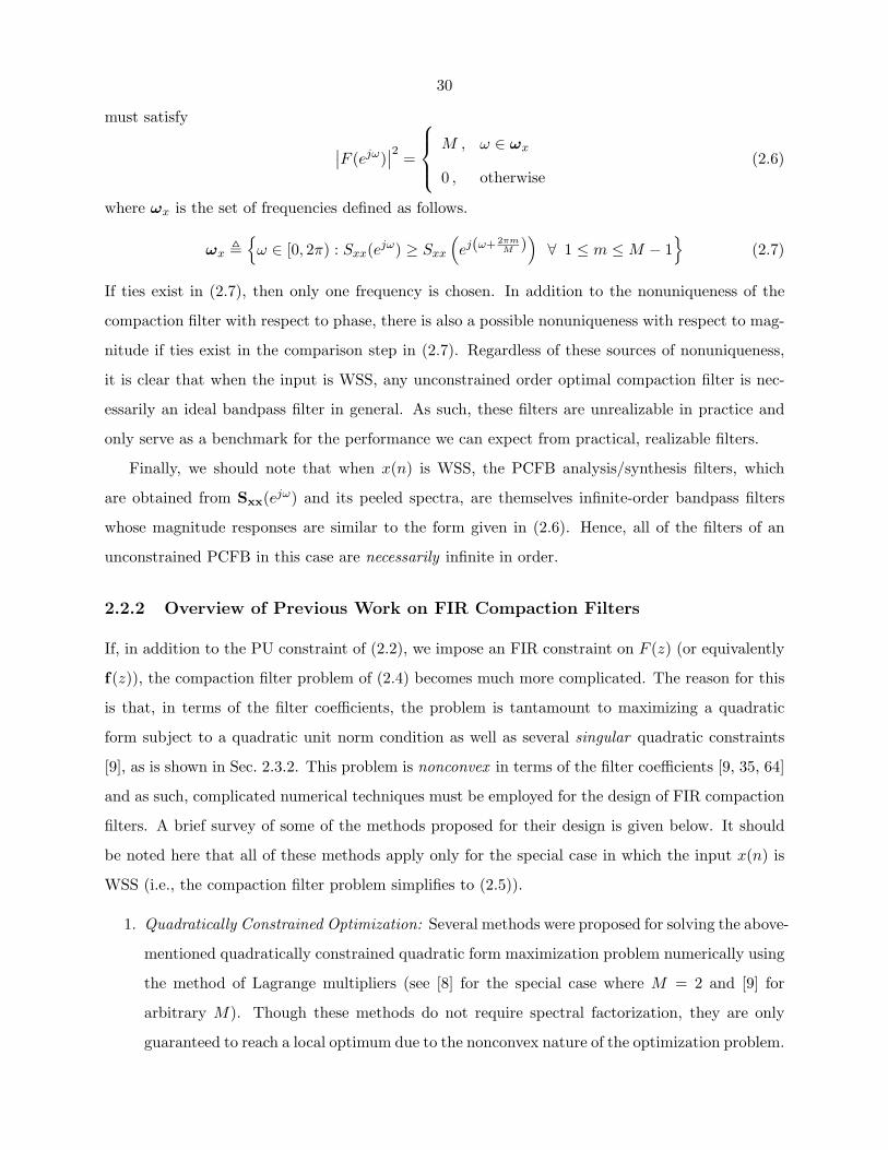
30

must satisfy ∣∣F (ejω)∣∣2 =

M , ω ∈ ωx

0 , otherwise(2.6)

where ωx is the set of frequencies defined as follows.

ωx �{

ω ∈ [0, 2π) : Sxx(ejω) ≥ Sxx

(ej(ω+ 2πm

M ))

∀ 1 ≤ m ≤ M − 1}

(2.7)

If ties exist in (2.7), then only one frequency is chosen. In addition to the nonuniqueness of the

compaction filter with respect to phase, there is also a possible nonuniqueness with respect to mag-

nitude if ties exist in the comparison step in (2.7). Regardless of these sources of nonuniqueness,

it is clear that when the input is WSS, any unconstrained order optimal compaction filter is nec-

essarily an ideal bandpass filter in general. As such, these filters are unrealizable in practice and

only serve as a benchmark for the performance we can expect from practical, realizable filters.

Finally, we should note that when x(n) is WSS, the PCFB analysis/synthesis filters, which

are obtained from Sxx(ejω) and its peeled spectra, are themselves infinite-order bandpass filters

whose magnitude responses are similar to the form given in (2.6). Hence, all of the filters of an

unconstrained PCFB in this case are necessarily infinite in order.

2.2.2 Overview of Previous Work on FIR Compaction Filters

If, in addition to the PU constraint of (2.2), we impose an FIR constraint on F (z) (or equivalently

f(z)), the compaction filter problem of (2.4) becomes much more complicated. The reason for this

is that, in terms of the filter coefficients, the problem is tantamount to maximizing a quadratic

form subject to a quadratic unit norm condition as well as several singular quadratic constraints

[9], as is shown in Sec. 2.3.2. This problem is nonconvex in terms of the filter coefficients [9, 35, 64]

and as such, complicated numerical techniques must be employed for the design of FIR compaction

filters. A brief survey of some of the methods proposed for their design is given below. It should

be noted here that all of these methods apply only for the special case in which the input x(n) is

WSS (i.e., the compaction filter problem simplifies to (2.5)).

1. Quadratically Constrained Optimization: Several methods were proposed for solving the above-

mentioned quadratically constrained quadratic form maximization problem numerically using

the method of Lagrange multipliers (see [8] for the special case where M = 2 and [9] for

arbitrary M). Though these methods do not require spectral factorization, they are only

guaranteed to reach a local optimum due to the nonconvex nature of the optimization problem.

31

2. Optimizing the FIR Lattice Structure: For the special case where M = 2, it is well known

that any real coefficient FIR PU filter bank is completely parameterized by a lattice structure

[67] which is characterized by a finite set of rotation angles. Several methods were proposed

for the optimization of these angles [70, 11]. Though these methods automatically satisfy

the desired PU constraint and do not require spectral factorization, they have the drawback

that they are only guaranteed to reach a local optimum and only work for the special case of

M = 2.

3. Optimizing the Product Filter: As the compaction filter problem of (2.5) is only in terms

of the magnitude squared response∣∣F (ejω)

∣∣2, several methods have been proposed for the

design of the product filter G(z) � F (z)F (z). In this case, the objective function σ2w becomes

linear in terms of the coefficients of G(z), but, in addition to the usual PU constraint of (2.2),

the positivity constraint G(ejω) ≥ 0 must be also be enforced. Hence, the problem is a linear

programming (LP) problem with infinitely many positivity inequality constraints (which is

typically called a semi-infinite programming (SIP) problem [35]). Several approaches were

proposed for finding the optimal product filter, including the window method of [29] and

the frequency discretization method of [35, 37], in which the positivity constraints are only

satisfied on a finite set of frequency points. These methods have been shown to yield good

performance, despite the fact that there is no guarantee of global optimality and a spectral

factorization step is required at the end.

4. State Space Approach: Recently an elegant method for the design of optimum FIR compaction

filters was proposed based on a state space description of the compaction filter [64]. This

method, which is based on a semi-definite programming (SDP) technique, ensures a globally

optimal compaction filter and doesn’t require a spectral factorization step. However, this

method only applies for WSS inputs x(n) and becomes extremely computationally intensive

as the filter order increases.

Using the proposed iterative eigenfilter method for the overdecimated filter bank model of Sec.

2.3, we can design several PCFB-like compaction filters simultaneously. Furthermore, since the

eigenfilter approach is used here, the method is very low in complexity [74, 56] and also can be

used when the input x(n) is CWSS(M).

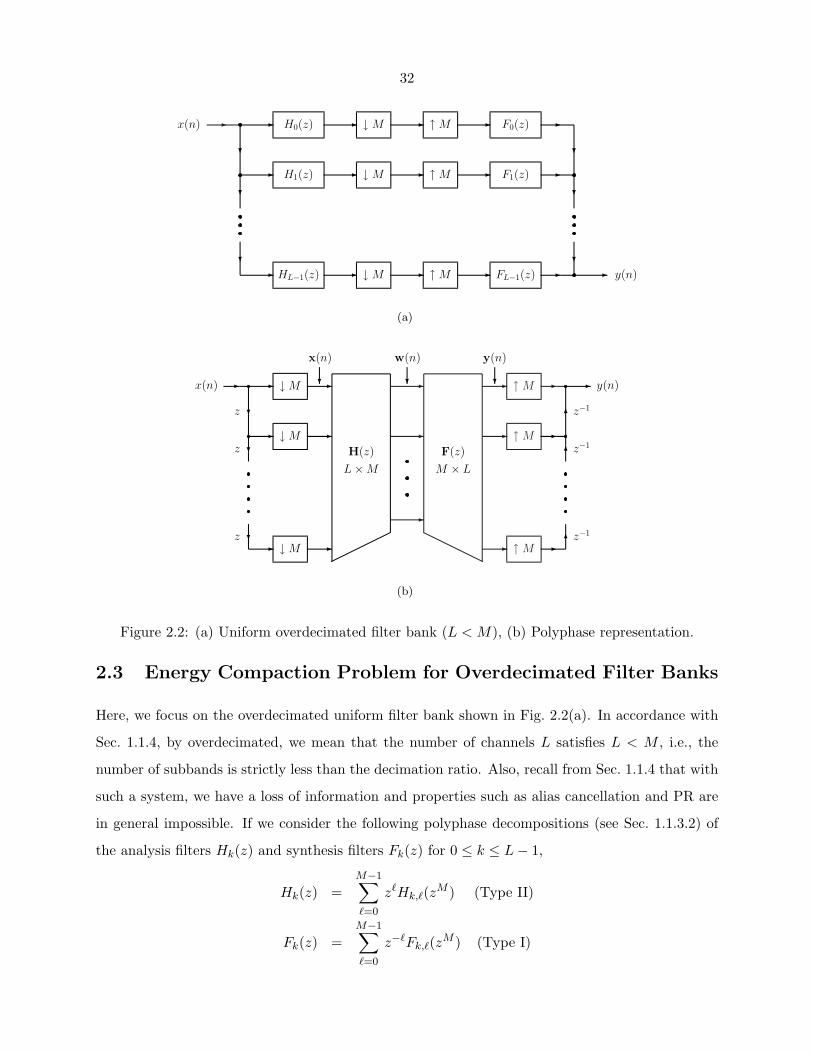
32

� �

�

�

H0(z)

H1(z)

HL−1(z)

�

�

�

�

�

�

↓ M

↓ M

↓ M

�

�

�

x(n) �

�

�

F0(z)

F1(z)

FL−1(z)

�

�

�

�

↑ M

↑ M

↑ M

�

�

� y(n)

(a)

�

�

�

�

�

�

↑ M

↑ M

↑ M

�

�

�

��

�

�

↓ M

↓ M

↓ M

�

�

�

�

�

�

�x(n) y(n)

z

z

z z−1

z−1

z−1

x(n)

�

y(n)

�

w(n)

�

F(z)

M × L

H(z)

L × M

(b)

Figure 2.2: (a) Uniform overdecimated filter bank (L < M), (b) Polyphase representation.

2.3 Energy Compaction Problem for Overdecimated Filter Banks

Here, we focus on the overdecimated uniform filter bank shown in Fig. 2.2(a). In accordance with

Sec. 1.1.4, by overdecimated, we mean that the number of channels L satisfies L < M , i.e., the

number of subbands is strictly less than the decimation ratio. Also, recall from Sec. 1.1.4 that with

such a system, we have a loss of information and properties such as alias cancellation and PR are

in general impossible. If we consider the following polyphase decompositions (see Sec. 1.1.3.2) of

the analysis filters Hk(z) and synthesis filters Fk(z) for 0 ≤ k ≤ L − 1,

Hk(z) =M−1∑�=0

z�Hk,�(zM ) (Type II)

Fk(z) =M−1∑�=0

z−�Fk,�(zM ) (Type I)

33

then the system of Fig. 2.2(a) can be redrawn as in Fig. 2.2(b), where

[H(z)]�,m = H�,m(z) , [F(z)]m,� = F�,m(z)

for 0 ≤ � ≤ L − 1 and 0 ≤ m ≤ M − 1. Note that here, the vector signals x(n) and y(n) denote,

respectively, the M -fold blocked versions [67] of the filter bank input x(n) and output y(n).

2.3.1 Derivation of the Energy Compaction Problem

Let us denote the autocorrelation sequence and psd of x(n) by Rxx(k) and Sxx(z), respectively.

In addition to this stationarity assumption on x(n), we will also assume that the filter bank is

orthonormal. This means that the matrices H(z) and F(z) from Fig. 2.2(b) satisfy [67]

H(z) = F(z) , F(z)F(z) = IL (2.8)

With the above assumptions on the input and filter bank, it can easily be shown that minimizing

the error of the output is equivalent to compacting the energy of the signal w(n).

Suppose that we wish to choose H(z) and F(z) subject to the orthonormality constraint of (2.8)

to minimize the expected mean-squared error between x(n) and y(n), defined as follows.

ξ � E[||x(n) − y(n)||2

](2.9)

If we define the blocked filter error e(n) as e(n) � x(n) − y(n) and denote the psd of e(n) by

See(z), then from (2.9), we have

ξ = Tr[E[e(n)e†(n)

]]=

12π

∫ 2π

0Tr[See(ejω)

]dω (2.10)

From Fig. 2.2(b) and [67], it can be shown that we have

See(z) = Sxx(z) − F(z)H(z)Sxx(z) − Sxx(z)H(z)F(z)

+ F(z)H(z)Sxx(z)H(z)F(z) (2.11)

Imposing the orthonormality constraint of (2.8) in (2.11) yields

Tr [See(z)] = Tr [Sxx(z)] − Tr[F(z)Sxx(z)F(z)

]Substituting this into (2.10) leads to the following.

ξ =12π

∫ 2π

0Tr[Sxx(ejω)

]dω

− 12π

∫ 2π

0Tr[F†(ejω)Sxx(ejω)F(ejω)

]dω︸ ︷︷ ︸

σ2w

(2.12)

= Tr [Rxx(0)] − σ2w (2.13)

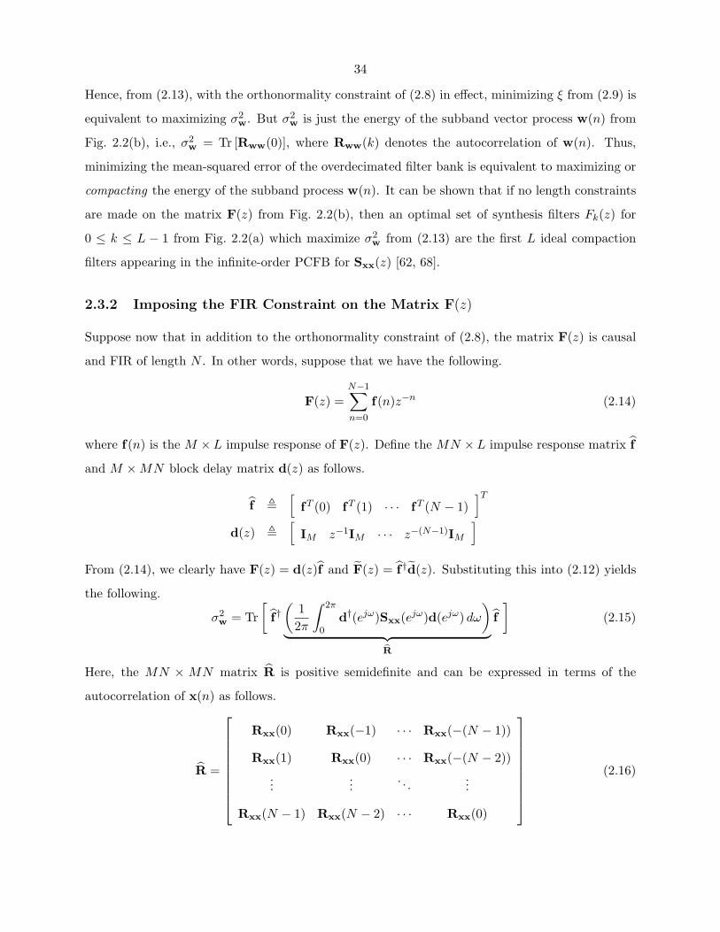
34

Hence, from (2.13), with the orthonormality constraint of (2.8) in effect, minimizing ξ from (2.9) is

equivalent to maximizing σ2w. But σ2

w is just the energy of the subband vector process w(n) from

Fig. 2.2(b), i.e., σ2w = Tr [Rww(0)], where Rww(k) denotes the autocorrelation of w(n). Thus,

minimizing the mean-squared error of the overdecimated filter bank is equivalent to maximizing or

compacting the energy of the subband process w(n). It can be shown that if no length constraints

are made on the matrix F(z) from Fig. 2.2(b), then an optimal set of synthesis filters Fk(z) for

0 ≤ k ≤ L − 1 from Fig. 2.2(a) which maximize σ2w from (2.13) are the first L ideal compaction

filters appearing in the infinite-order PCFB for Sxx(z) [62, 68].

2.3.2 Imposing the FIR Constraint on the Matrix F(z)

Suppose now that in addition to the orthonormality constraint of (2.8), the matrix F(z) is causal

and FIR of length N . In other words, suppose that we have the following.

F(z) =N−1∑n=0

f(n)z−n (2.14)

where f(n) is the M ×L impulse response of F(z). Define the MN ×L impulse response matrix f

and M × MN block delay matrix d(z) as follows.

f �[

fT (0) fT (1) · · · fT (N − 1)]T

d(z) �[

IM z−1IM · · · z−(N−1)IM

]From (2.14), we clearly have F(z) = d(z)f and F(z) = f †d(z). Substituting this into (2.12) yields

the following.

σ2w = Tr

[f †(

12π

∫ 2π

0d†(ejω)Sxx(ejω)d(ejω) dω

)︸ ︷︷ ︸

R

f]

(2.15)

Here, the MN × MN matrix R is positive semidefinite and can be expressed in terms of the

autocorrelation of x(n) as follows.

R =

Rxx(0) Rxx(−1) · · · Rxx(−(N − 1))

Rxx(1) Rxx(0) · · · Rxx(−(N − 2))...

.... . .

...

Rxx(N − 1) Rxx(N − 2) · · · Rxx(0)

(2.16)

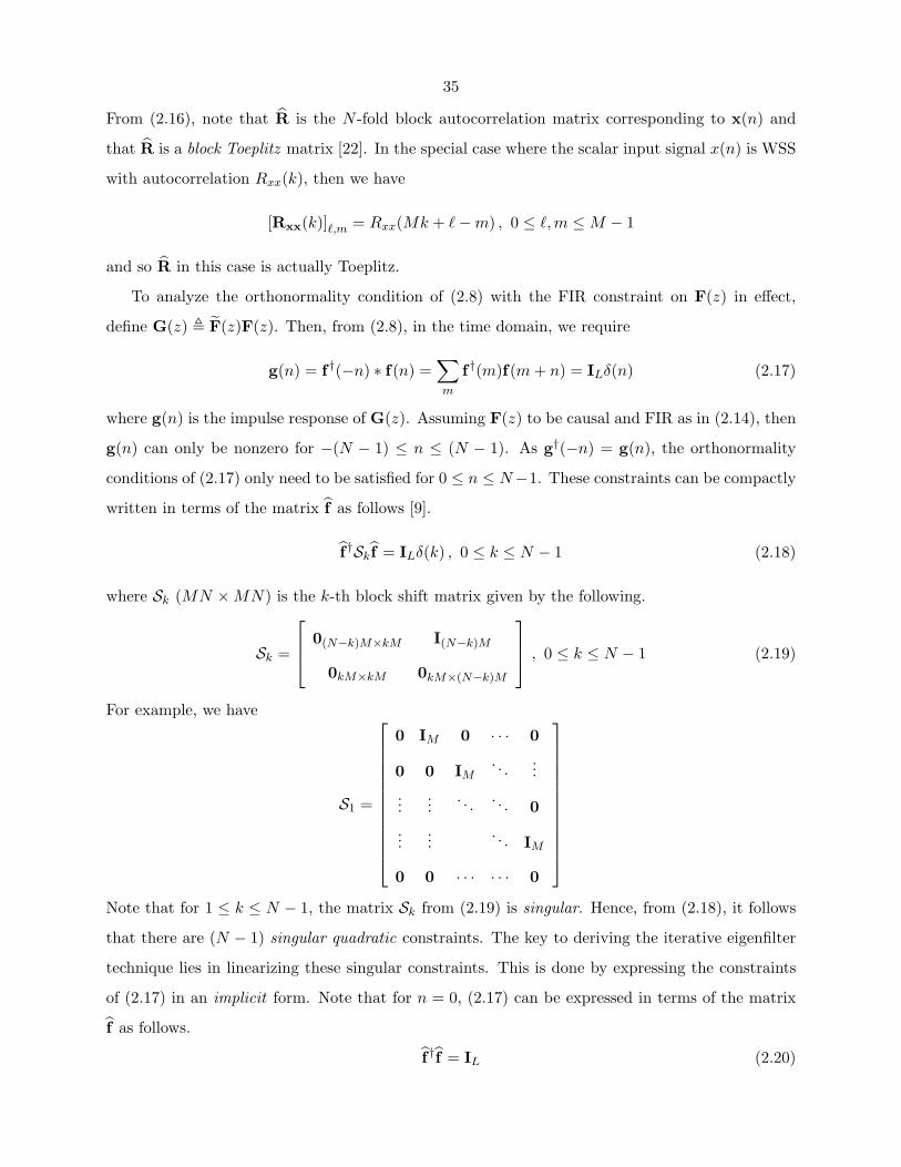
35

From (2.16), note that R is the N -fold block autocorrelation matrix corresponding to x(n) and

that R is a block Toeplitz matrix [22]. In the special case where the scalar input signal x(n) is WSS

with autocorrelation Rxx(k), then we have

[Rxx(k)]�,m = Rxx(Mk + � − m) , 0 ≤ �, m ≤ M − 1

and so R in this case is actually Toeplitz.

To analyze the orthonormality condition of (2.8) with the FIR constraint on F(z) in effect,

define G(z) � F(z)F(z). Then, from (2.8), in the time domain, we require

g(n) = f †(−n) ∗ f(n) =∑m

f †(m)f(m + n) = ILδ(n) (2.17)

where g(n) is the impulse response of G(z). Assuming F(z) to be causal and FIR as in (2.14), then

g(n) can only be nonzero for −(N − 1) ≤ n ≤ (N − 1). As g†(−n) = g(n), the orthonormality

conditions of (2.17) only need to be satisfied for 0 ≤ n ≤ N−1. These constraints can be compactly

written in terms of the matrix f as follows [9].

f †Sk f = ILδ(k) , 0 ≤ k ≤ N − 1 (2.18)

where Sk (MN × MN) is the k-th block shift matrix given by the following.

Sk =

0(N−k)M×kM I(N−k)M

0kM×kM 0kM×(N−k)M

, 0 ≤ k ≤ N − 1 (2.19)

For example, we have

S1 =

0 IM 0 · · · 0

0 0 IM. . .

......

.... . . . . . 0

......

. . . IM

0 0 · · · · · · 0

Note that for 1 ≤ k ≤ N − 1, the matrix Sk from (2.19) is singular. Hence, from (2.18), it follows

that there are (N − 1) singular quadratic constraints. The key to deriving the iterative eigenfilter

technique lies in linearizing these singular constraints. This is done by expressing the constraints

of (2.17) in an implicit form. Note that for n = 0, (2.17) can be expressed in terms of the matrix

f as follows.

f †f = IL (2.20)

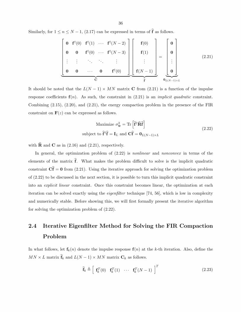
36

Similarly, for 1 ≤ n ≤ N − 1, (2.17) can be expressed in terms of f as follows.

0 f †(0) f †(1) · · · f †(N − 2)

0 0 f †(0) · · · f †(N − 3)...

.... . . . . .

...

0 0 · · · 0 f †(0)

︸ ︷︷ ︸

C

f(0)

f(1)...

f(N − 1)

︸ ︷︷ ︸

f

=

0

0...

0

︸ ︷︷ ︸

0L(N−1)×L

(2.21)

It should be noted that the L(N − 1) × MN matrix C from (2.21) is a function of the impulse

response coefficients f(n). As such, the constraint in (2.21) is an implicit quadratic constraint.

Combining (2.15), (2.20), and (2.21), the energy compaction problem in the presence of the FIR

constraint on F(z) can be expressed as follows.

Maximize σ2w = Tr

[f †Rf

]subject to f †f = IL and Cf = 0L(N−1)×L

(2.22)

with R and C as in (2.16) and (2.21), respectively.

In general, the optimization problem of (2.22) is nonlinear and nonconvex in terms of the

elements of the matrix f . What makes the problem difficult to solve is the implicit quadratic

constraint Cf = 0 from (2.21). Using the iterative approach for solving the optimization problem

of (2.22) to be discussed in the next section, it is possible to turn this implicit quadratic constraint

into an explicit linear constraint. Once this constraint becomes linear, the optimization at each

iteration can be solved exactly using the eigenfilter technique [74, 56], which is low in complexity

and numerically stable. Before showing this, we will first formally present the iterative algorithm

for solving the optimization problem of (2.22).

2.4 Iterative Eigenfilter Method for Solving the FIR Compaction

Problem

In what follows, let fk(n) denote the impulse response f(n) at the k-th iteration. Also, define the

MN × L matrix fk and L(N − 1) × MN matrix Ck as follows.

fk �[

fTk (0) fT

k (1) · · · fTk (N − 1)

]T(2.23)

37

Ck �

0 f †k(0) f †k(1) · · · f †k(N − 2)

0 0 f †k(0) · · · f †k(N − 3)...

.... . . . . .

...

0 0 · · · 0 f †k(0)

(2.24)

Then, the proposed iterative algorithm is as follows.

Initialization:

Choose any f0(n) which satisfies the orthonormality constraints of (2.17). This can be eas-

ily done using the complete characterization of FIR PU systems in terms of degree-one

Householder-like building blocks [75, 67]. Compute f0 from f0(n).

Iteration: For k ≥ 1, do the following.

1. Compute the constraint matrix Ck−1.

2. Solve the linearized optimization problem

Maximize σ2w,k = Tr

[f †kRfk

]subject to f †k fk = IL and Ck−1fk = 0L(N−1)×L

(2.25)

3. To measure the convergence of the iteration to an orthonormal solution, calculate the

orthonormality error matrix at the k-th iteration defined by

εk � Ck fk (2.26)

As we need εk = 0 in theory (from (2.21), (2.23), (2.24), and (2.26)), terminate the

iteration when we have

||εk||F < δT (2.27)

where ||εk||F denotes the Frobenius norm of εk [22] and δT is a some small threshold

value.

Before proceeding, it should be noted that there is no guarantee that the iterative algorithm

will converge to an orthonormal solution, although in simulations it often does so as shown below.

At present, there is no known method as to what should be done if the iteration fails to converge

to an orthonormal solution. Furthermore, even if there is convergence, there is no guarantee that

the resulting solution is globally optimal.

38

Despite this, often times in simulations such as those presented below, the algorithm performs

well in terms of approaching the behavior of the ideal compaction filters of the infinite-order PCFB.

Also, the algorithm can be used for relatively large orders N , as the linearized optimization problem

of (2.25) can be solved using the eigenfilter approach [67]. We now proceed to show how to solve

the linearized optimization problem of (2.25).

2.4.1 Solution to the Iterative Linearized Optimization Problem

Consider the linear constraint Ck−1fk = 0 from (2.25). This constraint holds iff the columns of fk

lie in the null space of Ck−1 [22]. Let Uk−1 denote a unitary matrix whose columns span the null

space of Ck−1. If ρ denotes the dimension of the null space of Ck−1, then Uk−1 is MN × ρ. As

the columns of fk must lie in the null space of Ck−1, fk must be of the form fk = Uk−1a for some

arbitrary ρ × L matrix a. Hence, we have

Ck−1fk = 0 ⇐⇒ fk = Uk−1a (2.28)

Given that Ck−1 is L(N − 1) × MN , we can easily argue that the dimension of its null space ρ

satisfies ρ ≥ L. Hence, the linear constraint Ck−1fk = 0 transforms the problem of finding fk into

that of finding the ρ × L matrix a. The quantity a is arbitrary but must be such that the unitary

constraint f †k fk = IL from (2.25) is satisfied. Clearly, from (2.28), we have

f †k fk = IL ⇐⇒ a†a = IL

upon exploiting the unitarity of Uk−1. As can be seen, the constraints of (2.25) transform the

problem of finding fk into that of finding a where a is allowed to by any ρ × L unitary matrix.

Hence, the optimization problem of (2.25) can be recast as follows.

Maximize σ2w,k = Tr

[a†Rk−1a

]where Rk−1 � U†

k−1RUk−1

subject to the constraint a†a = IL

(2.29)

The solution to this problem follows from a generalization of Rayleigh’s principle [22, p. 191] and

is as follows. Suppose that Rk−1 has the following unitary diagonalization.

Rk−1 = Vk−1Λk−1V†k−1

where Vk−1 is a ρ × ρ matrix of eigenvectors of Rk−1 and Λk−1 is a diagonal matrix consisting of

the eigenvalues of Rk−1. In addition, suppose that Λk−1 = diag (λk−1,0, λk−1,1, . . . , λk−1,ρ−1) and

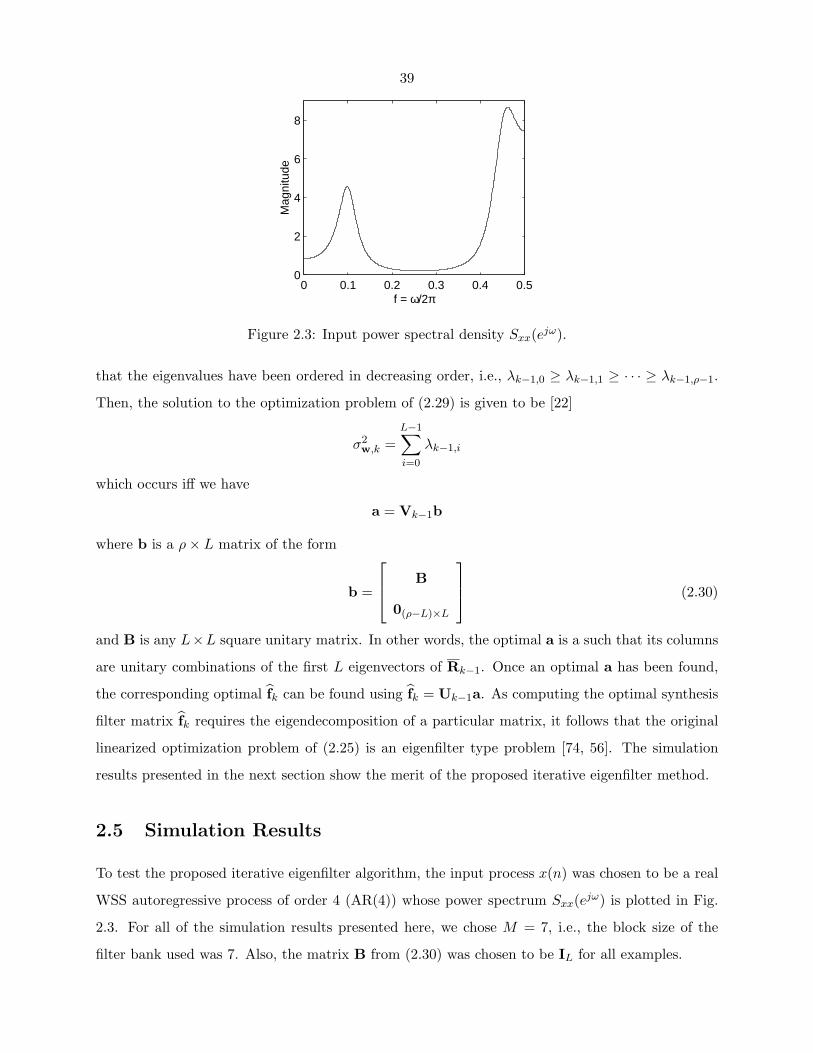
39

0 0.1 0.2 0.3 0.4 0.50

2

4

6

8

f = ω/2πM

agni

tude

Figure 2.3: Input power spectral density Sxx(ejω).

that the eigenvalues have been ordered in decreasing order, i.e., λk−1,0 ≥ λk−1,1 ≥ · · · ≥ λk−1,ρ−1.

Then, the solution to the optimization problem of (2.29) is given to be [22]

σ2w,k =

L−1∑i=0

λk−1,i

which occurs iff we have

a = Vk−1b

where b is a ρ × L matrix of the form

b =

B

0(ρ−L)×L

(2.30)

and B is any L×L square unitary matrix. In other words, the optimal a is a such that its columns

are unitary combinations of the first L eigenvectors of Rk−1. Once an optimal a has been found,

the corresponding optimal fk can be found using fk = Uk−1a. As computing the optimal synthesis

filter matrix fk requires the eigendecomposition of a particular matrix, it follows that the original

linearized optimization problem of (2.25) is an eigenfilter type problem [74, 56]. The simulation

results presented in the next section show the merit of the proposed iterative eigenfilter method.

2.5 Simulation Results

To test the proposed iterative eigenfilter algorithm, the input process x(n) was chosen to be a real

WSS autoregressive process of order 4 (AR(4)) whose power spectrum Sxx(ejω) is plotted in Fig.

2.3. For all of the simulation results presented here, we chose M = 7, i.e., the block size of the

filter bank used was 7. Also, the matrix B from (2.30) was chosen to be IL for all examples.

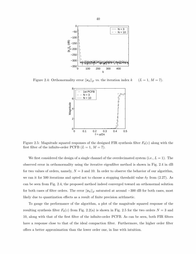
40

0 100 200 300 400−350

−300

−250

−200

−150

−100

−50

0

k||ε

k|| F (

dB)

N = 3N = 10

Figure 2.4: Orthonormality error ||εk||F vs. the iteration index k (L = 1, M = 7).

0 0.1 0.2 0.3 0.4 0.50

2

4

6

8

f = ω/2π

Mag

nitu

de

1st PCFBN = 3N = 10

Figure 2.5: Magnitude squared responses of the designed FIR synthesis filter F0(z) along with thefirst filter of the infinite-order PCFB (L = 1, M = 7).

We first considered the design of a single channel of the overdecimated system (i.e., L = 1). The

observed error in orthonormality using the iterative eigenfilter method is shown in Fig. 2.4 in dB

for two values of orders, namely, N = 3 and 10. In order to observe the behavior of our algorithm,

we ran it for 500 iterations and opted not to choose a stopping threshold value δT from (2.27). As

can be seen from Fig. 2.4, the proposed method indeed converged toward an orthonormal solution

for both cases of filter orders. The error ||εk||F saturated at around −300 dB for both cases, most

likely due to quantization effects as a result of finite precision arithmetic.

To gauge the performance of the algorithm, a plot of the magnitude squared response of the

resulting synthesis filter F0(z) from Fig. 2.2(a) is shown in Fig. 2.5 for the two orders N = 3 and

10, along with that of the first filter of the infinite-order PCFB. As can be seen, both FIR filters

have a response close to that of the ideal compaction filter. Furthermore, the higher order filter

offers a better approximation than the lower order one, in line with intuition.

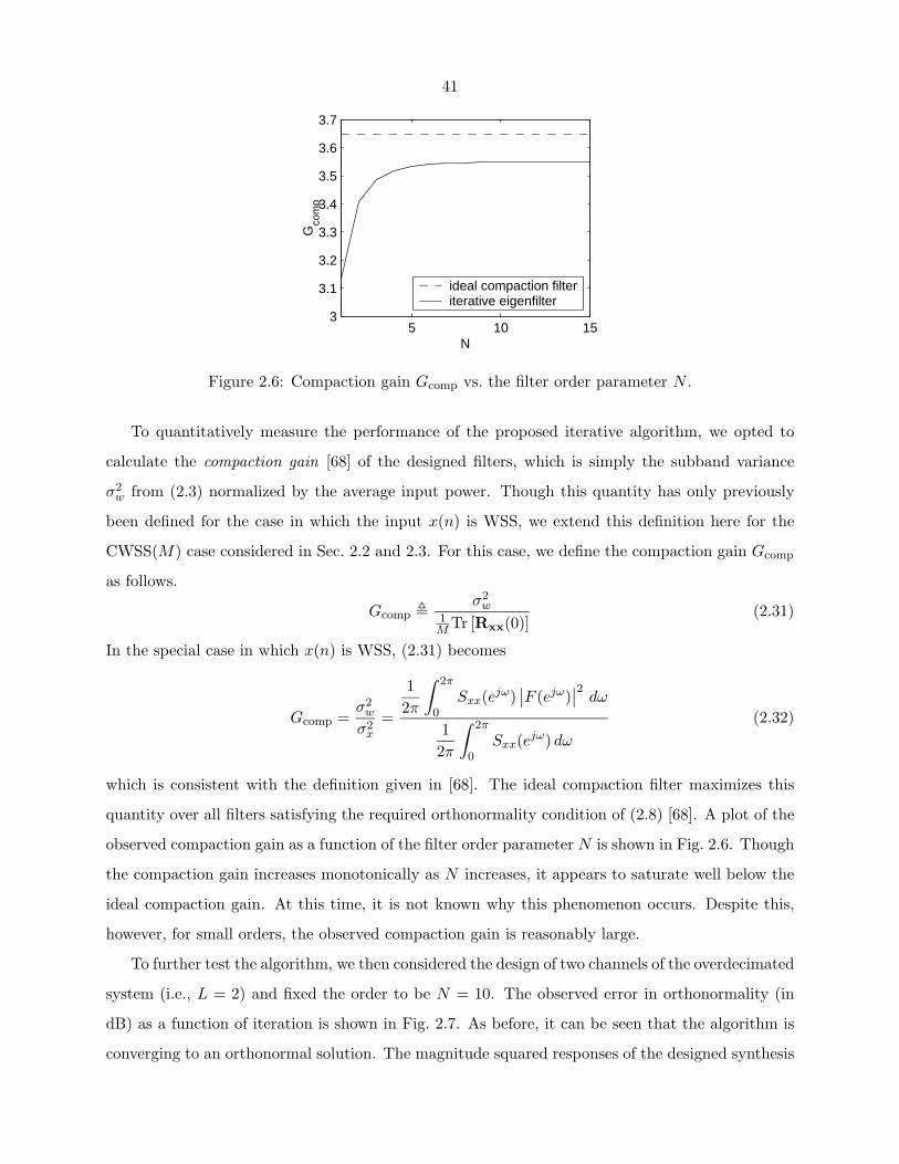
41

5 10 153

3.1

3.2

3.3

3.4

3.5

3.6

3.7

N

Gco

mp

ideal compaction filteriterative eigenfilter

Figure 2.6: Compaction gain Gcomp vs. the filter order parameter N .

To quantitatively measure the performance of the proposed iterative algorithm, we opted to

calculate the compaction gain [68] of the designed filters, which is simply the subband variance

σ2w from (2.3) normalized by the average input power. Though this quantity has only previously

been defined for the case in which the input x(n) is WSS, we extend this definition here for the

CWSS(M) case considered in Sec. 2.2 and 2.3. For this case, we define the compaction gain Gcomp

as follows.

Gcomp � σ2w

1M Tr [Rxx(0)]

(2.31)

In the special case in which x(n) is WSS, (2.31) becomes

Gcomp =σ2

w

σ2x

=

12π

∫ 2π

0Sxx(ejω)

∣∣F (ejω)∣∣2 dω

12π

∫ 2π

0Sxx(ejω) dω

(2.32)

which is consistent with the definition given in [68]. The ideal compaction filter maximizes this

quantity over all filters satisfying the required orthonormality condition of (2.8) [68]. A plot of the

observed compaction gain as a function of the filter order parameter N is shown in Fig. 2.6. Though

the compaction gain increases monotonically as N increases, it appears to saturate well below the

ideal compaction gain. At this time, it is not known why this phenomenon occurs. Despite this,

however, for small orders, the observed compaction gain is reasonably large.

To further test the algorithm, we then considered the design of two channels of the overdecimated

system (i.e., L = 2) and fixed the order to be N = 10. The observed error in orthonormality (in

dB) as a function of iteration is shown in Fig. 2.7. As before, it can be seen that the algorithm is

converging to an orthonormal solution. The magnitude squared responses of the designed synthesis

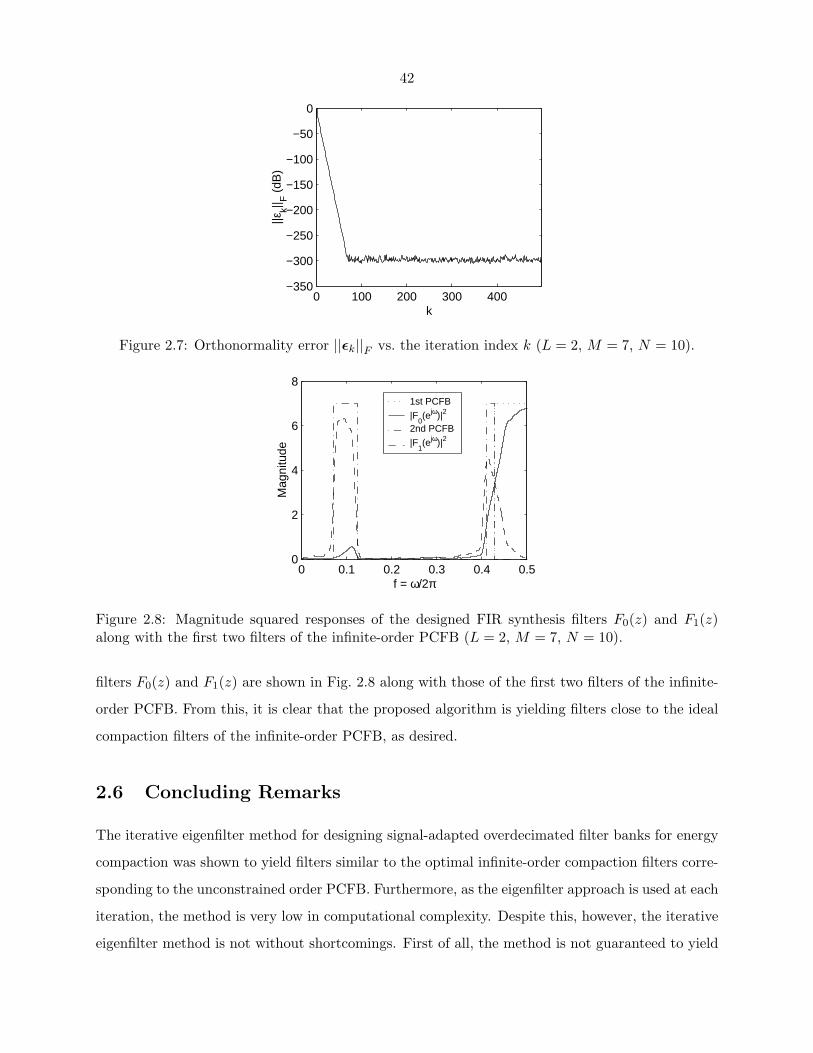
42

0 100 200 300 400−350

−300

−250

−200

−150

−100

−50

0

k

||εk|| F

(dB

)

Figure 2.7: Orthonormality error ||εk||F vs. the iteration index k (L = 2, M = 7, N = 10).

0 0.1 0.2 0.3 0.4 0.50

2

4

6

8

f = ω/2π

Mag

nitu

de

1st PCFB

|F0(ejω)|

2

2nd PCFB

|F1(ejω)|

2

Figure 2.8: Magnitude squared responses of the designed FIR synthesis filters F0(z) and F1(z)along with the first two filters of the infinite-order PCFB (L = 2, M = 7, N = 10).

filters F0(z) and F1(z) are shown in Fig. 2.8 along with those of the first two filters of the infinite-

order PCFB. From this, it is clear that the proposed algorithm is yielding filters close to the ideal

compaction filters of the infinite-order PCFB, as desired.

2.6 Concluding Remarks

The iterative eigenfilter method for designing signal-adapted overdecimated filter banks for energy

compaction was shown to yield filters similar to the optimal infinite-order compaction filters corre-

sponding to the unconstrained order PCFB. Furthermore, as the eigenfilter approach is used at each

iteration, the method is very low in computational complexity. Despite this, however, the iterative

eigenfilter method is not without shortcomings. First of all, the method is not guaranteed to yield

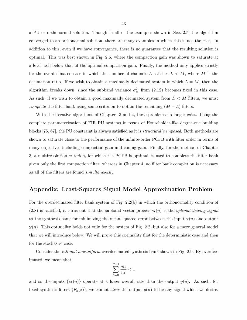
43

a PU or orthonormal solution. Though in all of the examples shown in Sec. 2.5, the algorithm

converged to an orthonormal solution, there are many examples in which this is not the case. In

addition to this, even if we have convergence, there is no guarantee that the resulting solution is

optimal. This was best shown in Fig. 2.6, where the compaction gain was shown to saturate at

a level well below that of the optimal compaction gain. Finally, the method only applies strictly

for the overdecimated case in which the number of channels L satisfies L < M , where M is the

decimation ratio. If we wish to obtain a maximally decimated system in which L = M , then the

algorithm breaks down, since the subband variance σ2w from (2.12) becomes fixed in this case.

As such, if we wish to obtain a good maximally decimated system from L < M filters, we must

complete the filter bank using some criterion to obtain the remaining (M − L) filters.

With the iterative algorithms of Chapters 3 and 4, these problems no longer exist. Using the

complete parameterization of FIR PU systems in terms of Householder-like degree-one building

blocks [75, 67], the PU constraint is always satisfied as it is structurally imposed. Both methods are

shown to saturate close to the performance of the infinite-order PCFB with filter order in terms of

many objectives including compaction gain and coding gain. Finally, for the method of Chapter

3, a multiresolution criterion, for which the PCFB is optimal, is used to complete the filter bank

given only the first compaction filter, whereas in Chapter 4, no filter bank completion is necessary

as all of the filters are found simultaneously.

Appendix: Least-Squares Signal Model Approximation Problem

For the overdecimated filter bank system of Fig. 2.2(b) in which the orthonormality condition of

(2.8) is satisfied, it turns out that the subband vector process w(n) is the optimal driving signal

to the synthesis bank for minimizing the mean-squared error between the input x(n) and output

y(n). This optimality holds not only for the system of Fig. 2.2, but also for a more general model

that we will introduce below. We will prove this optimality first for the deterministic case and then

for the stochastic case.

Consider the rational nonuniform overdecimated synthesis bank shown in Fig. 2.9. By overdec-

imated, we mean thatP−1∑k=0

mk

nk< 1

and so the inputs {ck(n)} operate at a lower overall rate than the output y(n). As such, for

fixed synthesis filters {Fk(z)}, we cannot steer the output y(n) to be any signal which we desire.

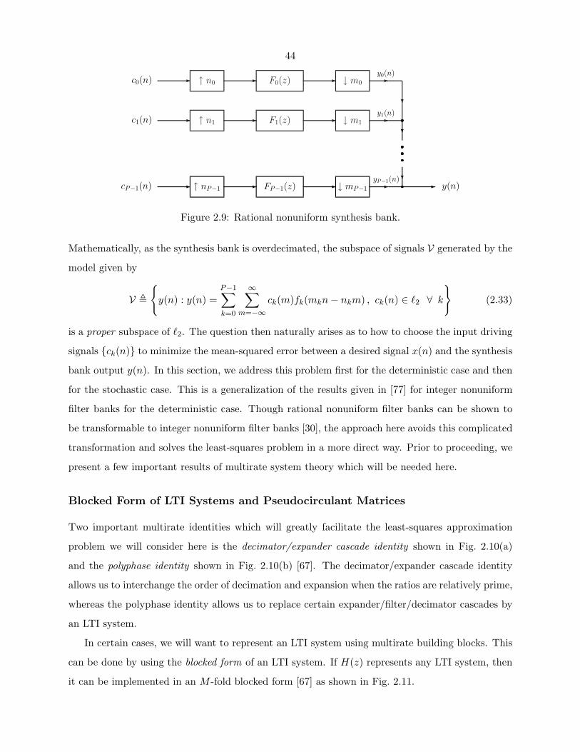
44

� ↑ n0 � F0(z) � ↓ m0 �

�

� ↑ n1 � F1(z) � ↓ m1 �

�

�� ↑ nP−1 � FP−1(z) � ↓ mP−1 � �

c0(n)

c1(n)

cP−1(n)

y0(n)

y1(n)

yP−1(n)y(n)

Figure 2.9: Rational nonuniform synthesis bank.

Mathematically, as the synthesis bank is overdecimated, the subspace of signals V generated by the

model given by

V �{

y(n) : y(n) =P−1∑k=0

∞∑m=−∞

ck(m)fk(mkn − nkm) , ck(n) ∈ �2 ∀ k

}(2.33)

is a proper subspace of �2. The question then naturally arises as to how to choose the input driving

signals {ck(n)} to minimize the mean-squared error between a desired signal x(n) and the synthesis

bank output y(n). In this section, we address this problem first for the deterministic case and then

for the stochastic case. This is a generalization of the results given in [77] for integer nonuniform

filter banks for the deterministic case. Though rational nonuniform filter banks can be shown to

be transformable to integer nonuniform filter banks [30], the approach here avoids this complicated

transformation and solves the least-squares problem in a more direct way. Prior to proceeding, we

present a few important results of multirate system theory which will be needed here.

Blocked Form of LTI Systems and Pseudocirculant Matrices

Two important multirate identities which will greatly facilitate the least-squares approximation

problem we will consider here is the decimator/expander cascade identity shown in Fig. 2.10(a)

and the polyphase identity shown in Fig. 2.10(b) [67]. The decimator/expander cascade identity

allows us to interchange the order of decimation and expansion when the ratios are relatively prime,

whereas the polyphase identity allows us to replace certain expander/filter/decimator cascades by

an LTI system.

In certain cases, we will want to represent an LTI system using multirate building blocks. This

can be done by using the blocked form of an LTI system. If H(z) represents any LTI system, then

it can be implemented in an M -fold blocked form [67] as shown in Fig. 2.11.

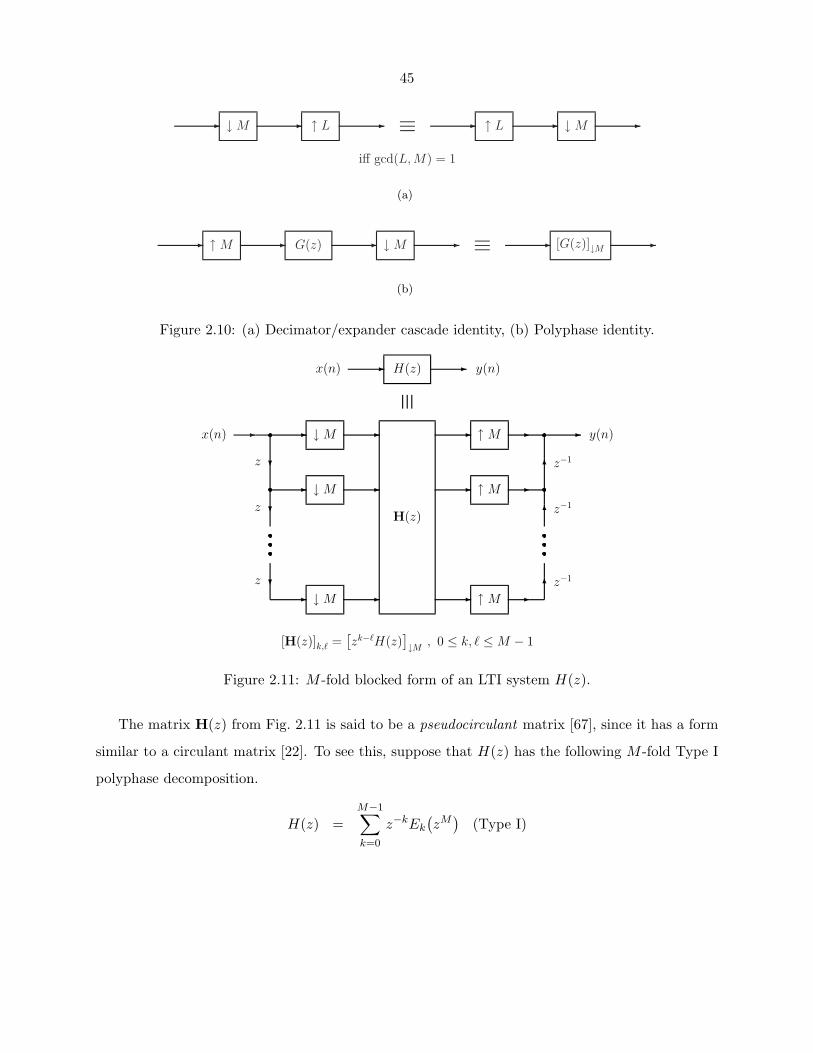
45

� ↓ M � ↑ L � ≡ � ↑ L � ↓ M �

iff gcd(L, M) = 1

(a)

� ↑ M � G(z) � ↓ M � ≡ � [G(z)]↓M �

(b)

Figure 2.10: (a) Decimator/expander cascade identity, (b) Polyphase identity.

� �

�

�

↓ M

↓ M

↓ M

�z

�z

�z

�

�

�

H(z)

�

�

�

x(n)

H(z)� �x(n) y(n)

�

�

�

z−1

z−1

z−1

�↑ M

↑ M

↑ M

y(n)

[H(z)]k,� =[zk−�H(z)

]↓M , 0 ≤ k, � ≤ M − 1

Figure 2.11: M -fold blocked form of an LTI system H(z).

The matrix H(z) from Fig. 2.11 is said to be a pseudocirculant matrix [67], since it has a form

similar to a circulant matrix [22]. To see this, suppose that H(z) has the following M -fold Type I

polyphase decomposition.

H(z) =M−1∑k=0

z−kEk

(zM

)(Type I)

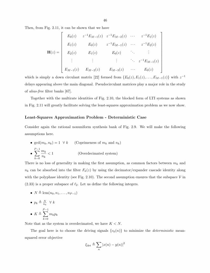
46

Then, from Fig. 2.11, it can be shown that we have

H(z) =

E0(z) z−1EM−1(z) z−1EM−2(z) · · · z−1E1(z)

E1(z) E0(z) z−1EM−1(z) · · · z−1E2(z)

E2(z) E1(z) E0(z). . .

......

......

. . . z−1EM−1(z)

EM−1(z) EM−2(z) EM−3(z) · · · E0(z)

which is simply a down circulant matrix [22] formed from {E0(z), E1(z), . . . , EM−1(z)} with z−1

delays appearing above the main diagonal. Pseudocirculant matrices play a major role in the study

of alias-free filter banks [67].

Together with the multirate identities of Fig. 2.10, the blocked form of LTI systems as shown

in Fig. 2.11 will greatly facilitate solving the least-squares approximation problem as we now show.

Least-Squares Approximation Problem - Deterministic Case

Consider again the rational nonuniform synthesis bank of Fig. 2.9. We will make the following

assumptions here.

• gcd(mk, nk) = 1 ∀ k (Coprimeness of mk and nk)

•P−1∑k=0

mk

nk< 1 (Overdecimated system)

There is no loss of generality in making the first assumption, as common factors between mk and

nk can be absorbed into the filter Fk(z) by using the decimator/expander cascade identity along

with the polyphase identity (see Fig. 2.10). The second assumption ensures that the subspace V in

(2.33) is a proper subspace of �2. Let us define the following integers.

• N � lcm(n0, n1, . . . , nP−1)

• pk � Nnk

∀ k

• K �P−1∑k=0

mkpk

Note that as the system is overdecimated, we have K < N .

The goal here is to choose the driving signals {ck(n)} to minimize the deterministic mean-

squared error objective

ξdet �∑

n

|x(n) − y(n)|2

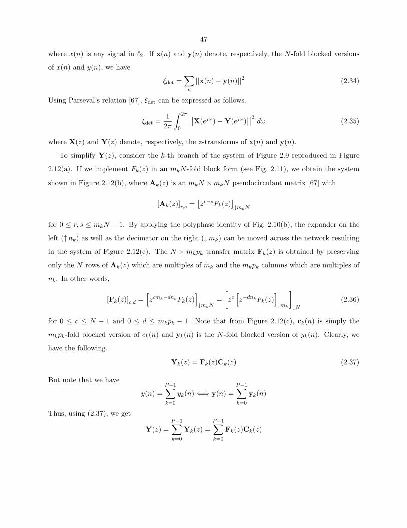
47

where x(n) is any signal in �2. If x(n) and y(n) denote, respectively, the N -fold blocked versions

of x(n) and y(n), we have

ξdet =∑

n

||x(n) − y(n)||2 (2.34)

Using Parseval’s relation [67], ξdet can be expressed as follows.

ξdet =12π

∫ 2π

0

∣∣∣∣X(ejω) − Y(ejω)∣∣∣∣2 dω (2.35)

where X(z) and Y(z) denote, respectively, the z-transforms of x(n) and y(n).

To simplify Y(z), consider the k-th branch of the system of Figure 2.9 reproduced in Figure

2.12(a). If we implement Fk(z) in an mkN -fold block form (see Fig. 2.11), we obtain the system

shown in Figure 2.12(b), where Ak(z) is an mkN × mkN pseudocirculant matrix [67] with

[Ak(z)]r,s =[zr−sFk(z)

]↓mkN

for 0 ≤ r, s ≤ mkN − 1. By applying the polyphase identity of Fig. 2.10(b), the expander on the

left (↑nk) as well as the decimator on the right (↓mk) can be moved across the network resulting

in the system of Figure 2.12(c). The N × mkpk transfer matrix Fk(z) is obtained by preserving

only the N rows of Ak(z) which are multiples of mk and the mkpk columns which are multiples of

nk. In other words,

[Fk(z)]c,d =[zcmk−dnkFk(z)

]↓mkN

=[zc[z−dnkFk(z)

]↓mk

]↓N

(2.36)

for 0 ≤ c ≤ N − 1 and 0 ≤ d ≤ mkpk − 1. Note that from Figure 2.12(c), ck(n) is simply the

mkpk-fold blocked version of ck(n) and yk(n) is the N -fold blocked version of yk(n). Clearly, we

have the following.

Yk(z) = Fk(z)Ck(z) (2.37)

But note that we have

y(n) =P−1∑k=0

yk(n) ⇐⇒ y(n) =P−1∑k=0

yk(n)

Thus, using (2.37), we get

Y(z) =P−1∑k=0

Yk(z) =P−1∑k=0

Fk(z)Ck(z)

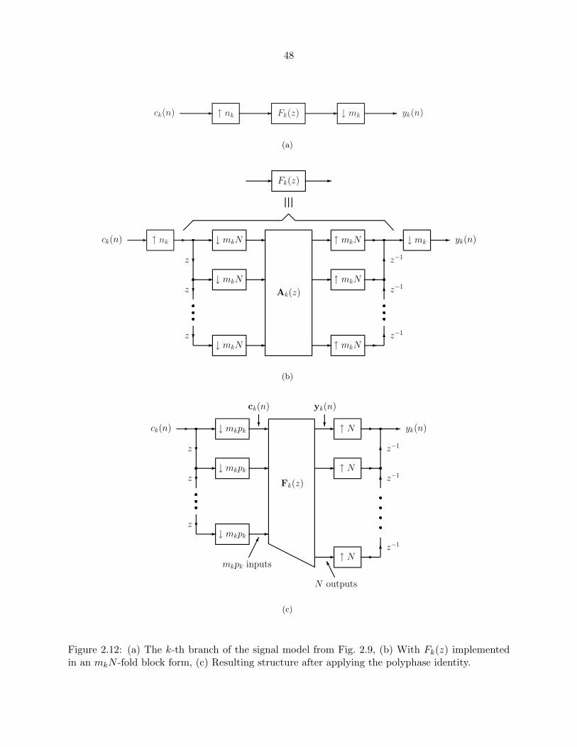
48

� ↑ nk� Fk(z) � ↓ mk

�ck(n) yk(n)

(a)

� ↑ nk� �

�

�

�

��

↓ mkN

↓ mkN

↓ mkN

�

�

�

Ak(z)

�

�

�

↑ mkN

↑ mkN

↑ mkN

�

�

�

� ↓ mk�ck(n) yk(n)

z

z

z z−1

z−1

z−1

Fk(z)� �

(b)

� �

�

�

�

��

↓ mkpk

↓ mkpk

↓ mkpk

�

�

�

�

�

�

↑ N

↑ N

↑ N

�

�

�

�ck(n) yk(n)

z

z

z

z−1

z−1

z−1

ck(n) yk(n)

� �

mkpk inputs

N outputs

�

Fk(z)

(c)

Figure 2.12: (a) The k-th branch of the signal model from Fig. 2.9, (b) With Fk(z) implementedin an mkN -fold block form, (c) Resulting structure after applying the polyphase identity.

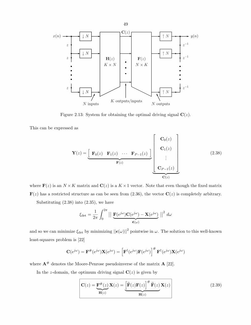
49

�

�

�

�

�

�

↑ N

↑ N

↑ N

�

�

�

��

�

�

↓ N

↓ N

↓ N

�

�

�

�

�

�

�x(n) y(n)

z

z

z z−1

z−1

z−1

C(z)

N inputs

K outputs/inputs

N outputs

�

F(z)

N × K

H(z)

K × N

Figure 2.13: System for obtaining the optimal driving signal C(z).

This can be expressed as

Y(z) =[

F0(z) F1(z) · · · FP−1(z)]

︸ ︷︷ ︸F(z)

C0(z)

C1(z)...

CP−1(z)

︸ ︷︷ ︸

C(z)

(2.38)

where F(z) is an N ×K matrix and C(z) is a K×1 vector. Note that even though the fixed matrix

F(z) has a restricted structure as can be seen from (2.36), the vector C(z) is completely arbitrary.

Substituting (2.38) into (2.35), we have

ξdet =12π

∫ 2π

0

∣∣∣∣ F(ejω)C(ejω) − X(ejω)︸ ︷︷ ︸ε(ω)

∣∣∣∣2 dω

and so we can minimize ξdet by minimizing ||ε(ω)||2 pointwise in ω. The solution to this well-known

least-squares problem is [22]

C(ejω) = F#(ejω)X(ejω) =[F†(ejω)F(ejω)

]#F†(ejω)X(ejω)

where A# denotes the Moore-Penrose pseudoinverse of the matrix A [22].

In the z-domain, the optimum driving signal C(z) is given by

C(z) = F#(z)︸ ︷︷ ︸H(z)

X(z) =[F(z)F(z)

]#F(z)︸ ︷︷ ︸

H(z)

X(z) (2.39)

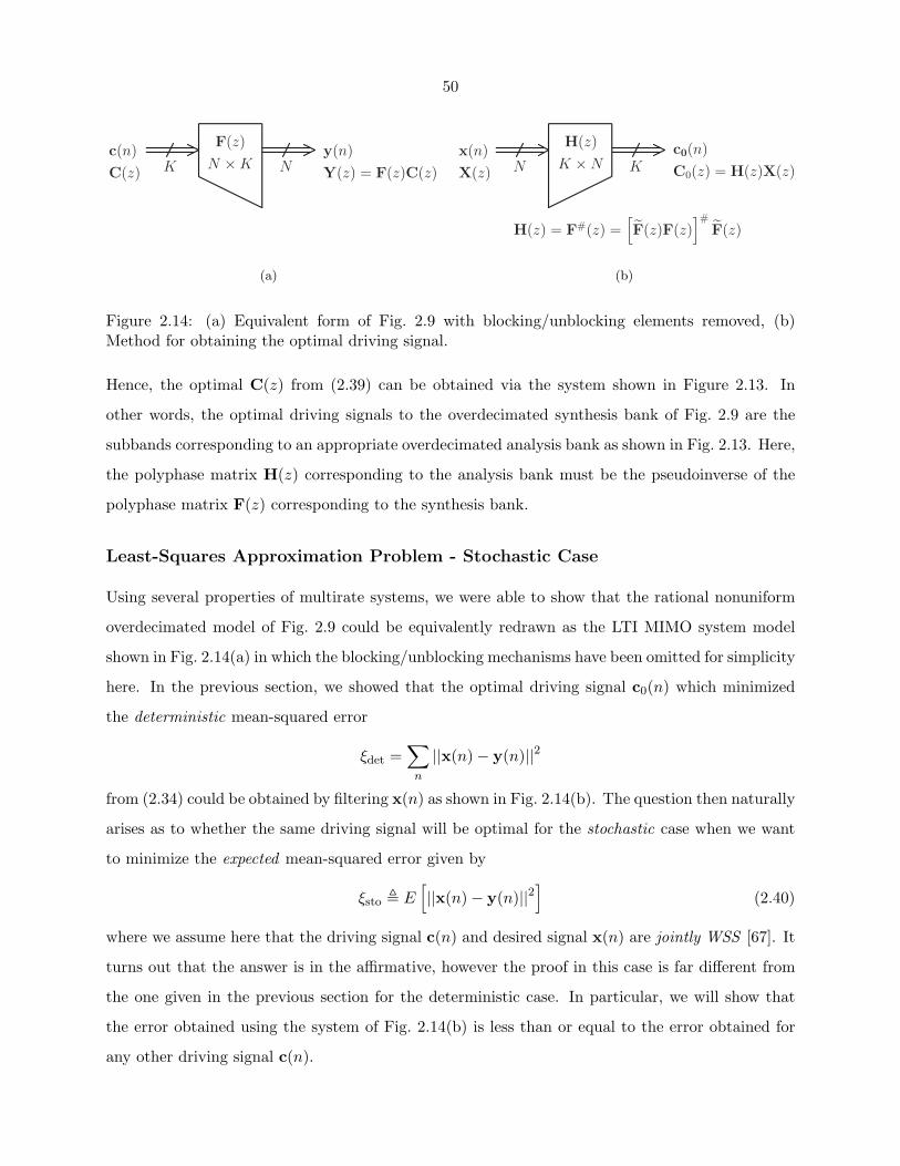
50

F(z)

N × KK Nc(n)

C(z)

y(n)

Y(z) = F(z)C(z)

(a)

H(z)

K × NN Kx(n)

X(z)

c0(n)

C0(z) = H(z)X(z)

H(z) = F#(z) =[F(z)F(z)

]#F(z)

(b)

Figure 2.14: (a) Equivalent form of Fig. 2.9 with blocking/unblocking elements removed, (b)Method for obtaining the optimal driving signal.

Hence, the optimal C(z) from (2.39) can be obtained via the system shown in Figure 2.13. In

other words, the optimal driving signals to the overdecimated synthesis bank of Fig. 2.9 are the

subbands corresponding to an appropriate overdecimated analysis bank as shown in Fig. 2.13. Here,

the polyphase matrix H(z) corresponding to the analysis bank must be the pseudoinverse of the

polyphase matrix F(z) corresponding to the synthesis bank.

Least-Squares Approximation Problem - Stochastic Case

Using several properties of multirate systems, we were able to show that the rational nonuniform

overdecimated model of Fig. 2.9 could be equivalently redrawn as the LTI MIMO system model

shown in Fig. 2.14(a) in which the blocking/unblocking mechanisms have been omitted for simplicity

here. In the previous section, we showed that the optimal driving signal c0(n) which minimized

the deterministic mean-squared error

ξdet =∑

n

||x(n) − y(n)||2

from (2.34) could be obtained by filtering x(n) as shown in Fig. 2.14(b). The question then naturally

arises as to whether the same driving signal will be optimal for the stochastic case when we want

to minimize the expected mean-squared error given by

ξsto � E[||x(n) − y(n)||2

](2.40)

where we assume here that the driving signal c(n) and desired signal x(n) are jointly WSS [67]. It

turns out that the answer is in the affirmative, however the proof in this case is far different from

the one given in the previous section for the deterministic case. In particular, we will show that

the error obtained using the system of Fig. 2.14(b) is less than or equal to the error obtained for

any other driving signal c(n).

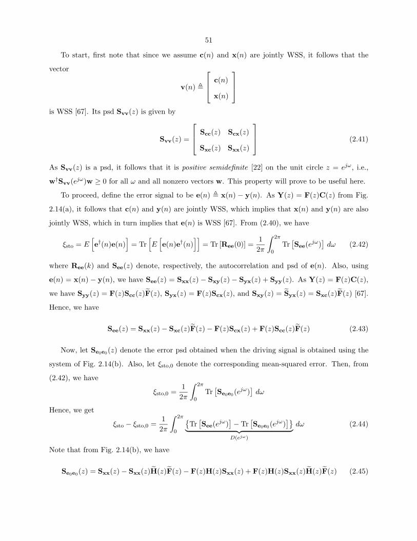
51

To start, first note that since we assume c(n) and x(n) are jointly WSS, it follows that the

vector

v(n) �

c(n)

x(n)

is WSS [67]. Its psd Svv(z) is given by

Svv(z) =

Scc(z) Scx(z)

Sxc(z) Sxx(z)

(2.41)

As Svv(z) is a psd, it follows that it is positive semidefinite [22] on the unit circle z = ejω, i.e.,

w†Svv(ejω)w ≥ 0 for all ω and all nonzero vectors w. This property will prove to be useful here.

To proceed, define the error signal to be e(n) � x(n) − y(n). As Y(z) = F(z)C(z) from Fig.

2.14(a), it follows that c(n) and y(n) are jointly WSS, which implies that x(n) and y(n) are also

jointly WSS, which in turn implies that e(n) is WSS [67]. From (2.40), we have

ξsto = E[e†(n)e(n)

]= Tr

[E[e(n)e†(n)

]]= Tr [Ree(0)] =

12π

∫ 2π

0Tr[See(ejω)

]dω (2.42)

where Ree(k) and See(z) denote, respectively, the autocorrelation and psd of e(n). Also, using

e(n) = x(n) − y(n), we have See(z) = Sxx(z) − Sxy(z) − Syx(z) + Syy(z). As Y(z) = F(z)C(z),

we have Syy(z) = F(z)Scc(z)F(z), Syx(z) = F(z)Scx(z), and Sxy(z) = Syx(z) = Sxc(z)F(z) [67].

Hence, we have

See(z) = Sxx(z) − Sxc(z)F(z) − F(z)Scx(z) + F(z)Scc(z)F(z) (2.43)

Now, let Se0e0(z) denote the error psd obtained when the driving signal is obtained using the

system of Fig. 2.14(b). Also, let ξsto,0 denote the corresponding mean-squared error. Then, from

(2.42), we have

ξsto,0 =12π

∫ 2π

0Tr[Se0e0(e

jω)]

dω

Hence, we get

ξsto − ξsto,0 =12π

∫ 2π

0

{Tr[See(ejω)

]− Tr[Se0e0(e

jω)]}︸ ︷︷ ︸

D(ejω)

dω (2.44)

Note that from Fig. 2.14(b), we have

Se0e0(z) = Sxx(z) − Sxx(z)H(z)F(z) − F(z)H(z)Sxx(z) + F(z)H(z)Sxx(z)H(z)F(z) (2.45)

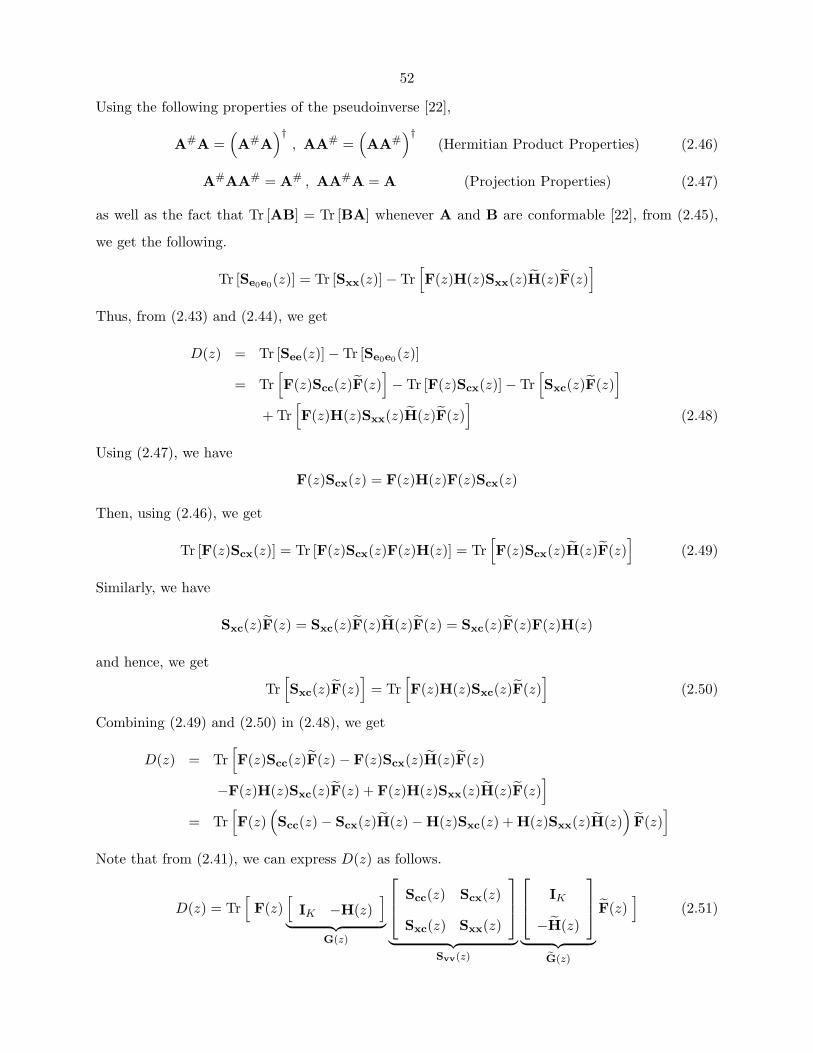
52

Using the following properties of the pseudoinverse [22],

A#A =(A#A

)†, AA# =

(AA#

)†(Hermitian Product Properties) (2.46)

A#AA# = A# , AA#A = A (Projection Properties) (2.47)

as well as the fact that Tr [AB] = Tr [BA] whenever A and B are conformable [22], from (2.45),

we get the following.

Tr [Se0e0(z)] = Tr [Sxx(z)] − Tr[F(z)H(z)Sxx(z)H(z)F(z)

]Thus, from (2.43) and (2.44), we get

D(z) = Tr [See(z)] − Tr [Se0e0(z)]

= Tr[F(z)Scc(z)F(z)

]− Tr [F(z)Scx(z)] − Tr

[Sxc(z)F(z)

]+ Tr

[F(z)H(z)Sxx(z)H(z)F(z)

](2.48)

Using (2.47), we have

F(z)Scx(z) = F(z)H(z)F(z)Scx(z)

Then, using (2.46), we get

Tr [F(z)Scx(z)] = Tr [F(z)Scx(z)F(z)H(z)] = Tr[F(z)Scx(z)H(z)F(z)

](2.49)

Similarly, we have

Sxc(z)F(z) = Sxc(z)F(z)H(z)F(z) = Sxc(z)F(z)F(z)H(z)

and hence, we get

Tr[Sxc(z)F(z)

]= Tr

[F(z)H(z)Sxc(z)F(z)

](2.50)

Combining (2.49) and (2.50) in (2.48), we get

D(z) = Tr[F(z)Scc(z)F(z) − F(z)Scx(z)H(z)F(z)

−F(z)H(z)Sxc(z)F(z) + F(z)H(z)Sxx(z)H(z)F(z)]

= Tr[F(z)

(Scc(z) − Scx(z)H(z) − H(z)Sxc(z) + H(z)Sxx(z)H(z)

)F(z)

]Note that from (2.41), we can express D(z) as follows.

D(z) = Tr[F(z)

[IK −H(z)

]︸ ︷︷ ︸

G(z)

Scc(z) Scx(z)

Sxc(z) Sxx(z)

︸ ︷︷ ︸

Svv(z)

IK

−H(z)

︸ ︷︷ ︸

G(z)

F(z)]

(2.51)

53

But recall that Svv(ejω) is positive semidefinite as it is the psd of v(n). Thus, from (2.51), we have

D(z) = Tr[F(z)G(z)Svv(z)G(z)F(z)︸ ︷︷ ︸positive semidefinite on z = ejω

]As the trace of any positive semidefinite matrix is nonnegative [22], D(ejω) ≥ 0. From (2.44), this

implies

ξsto − ξsto,0 =12π

∫ 2π

0D(ejω) dω ≥ 0 ⇐⇒ ξsto,0 ≤ ξsto

Hence, the error obtained using the system of Fig. 2.14(b) is always less than or equal to the error

obtained with any other driving signal. Thus, the driving signal c0(n) from Fig. 2.14(b) is always

an optimal driving signal and so the optimal driving signal in the deterministic case is also an

optimal driving signal in the stochastic case. In parting, the following comments are in order. If the synthesis polyphase matrix F(z) is PU,

i.e., F(z)F(z) = IK , then the optimal analysis bank H(z) = F#(z) =[F(z)F(z)

]#F(z) is simply

H(z) = F(z), i.e., H(z) is the paraconjugate of F(z). In this case, the resulting filter bank system

is orthonormal. The uniform PU filter bank of Fig. 2.2 is an example of such a filter bank.

In addition to this, with the optimal driving signal c(n), it can easily be shown that if F(z) is

PU, then minimizing the mean-squared error further by choice of F(z) is equivalent to compacting

the energy of c(n). To see this, note that with the optimal C(z) from (2.39), the mean-squared

error in the deterministic and stochastic cases are respectively given by (2.34) and (2.40) to be

ξdet =∑

n

|x(n)|2 − Tr[

12π

∫ 2π

0H(ejω)X(ejω)X†(ejω)F(ejω) dω

]︸ ︷︷ ︸

σ2c,det

ξsto = Tr [Rxx(0)] − Tr[

12π

∫ 2π

0H(ejω)Sxx(ejω)F(ejω) dω

]︸ ︷︷ ︸

σ2c,sto

where H(z) = F#(z). Clearly, minimizing ξdet and ξsto is equivalent to maximizing σ2c,det and σ2

c,sto,

respectively. If F(z) is PU, then H(z) = F(z) or equivalently F(z) = H(z). In this case, we get

σ2c,det = Tr

[12π

∫ 2π

0H(ejω)X(ejω)X†(ejω)H†(ejω) dω

]σ2c,det = Tr

[12π

∫ 2π

0H(ejω)Sxx(ejω)H†(ejω) dω

]which is simply the energy of the optimal driving signal from Fig. 2.14(b) for the deterministic

and stochastic cases, respectively. Hence, with the PU constraint in effect, minimizing the mean-

squared error is equivalent to compacting the energy of the subband vector process, as was shown

for the uniform case in Sec. 2.3.1.

54

Chapter 3

Multiresolution OptimalFIR PU Filter Banks

One major drawback of the iterative eigenfilter method of the previous chapter is that there is no

guarantee of convergence to a PU solution for the synthesis bank. In this chapter, an alternate

method for designing a compaction filter is proposed in which the PU constraint is structurally

imposed. This follows from the complete parameterization of all 1-D causal FIR PU systems in

terms of Householder-like degree-one building blocks [75, 67], which we review here.

Using this characterization, an iterative algorithm is proposed to approximate, in the least-

squares sense, any desired response by an FIR filter whose vector of polyphase components is PU.

At each iteration, one set of parameters in the characterization of the FIR PU system is globally

optimized assuming all other parameters to be fixed. As such, the resulting algorithm is greedy and

so the error is guaranteed to be monotonic nonincreasing with iteration.

When the desired response is the response of an optimal infinite-order compaction filter, the

algorithm can be used for the design of FIR compaction filters. As the desired response in this case

suffers from a phase ambiguity, which we show here, a modification to the algorithm is proposed

in which the phase of the FIR solution is fed back to the desired response. With this modification,

which we call the phase feedback modification, in effect, the iterative algorithm not only still remains

greedy, but also outperforms the unmodified one in terms of compaction gain. In simulations

provided, we show that when this modification is used, the compaction gain monotonically increases

with filter order and comes very close to the performance of the infinite-order compaction filter.

To complete a maximally decimated filter bank given an FIR compaction filter, a multiresolution

criterion [62, 37] for which the PCFB is optimal, is used. Using the above-mentioned characteriza-

tion of FIR PU systems, it can be shown that the entire filter bank can be elegantly designed with

55

only one FIR compaction filter followed by an appropriate KLT, as we review here. Though ele-

gant, this approach suffers from the nonuniqueness of the FIR compaction filter. Different spectral

factors of a given FIR compaction filter lead to different FIR PU filter banks which in turn yield

different performances in terms of certain objective functions. This phenomenon has not previously

been reported in the literature. By choosing the spectral factor which yields the largest coding gain,

in simulations, we show that as the filter order increases, the resulting FIR PU filter bank behaves

more and more like the unconstrained or infinite-order PCFB in terms of numerous objectives.

In particular, this behavior is shown for coding gain, multiresolution, denoising with zeroth-order

Wiener filters in the subbands, and power minimization in nonredundant PU transmultiplexers.

This serves to bridge the gap between the zeroth-order memory KLT and infinite-order PCFB,

which has not previously been reported in the literature.

Since all spectral factors of a given FIR compaction filter must be tested for performance, the

computational complexity grows exponentially with filter order. As such, designing FIR PU filter

banks using the multiresolution criterion of [62, 37] becomes less feasible as the filter order increases.

In essence, what we show here is that due to the inherent nonuniqueness of an FIR compaction

filter, the FIR compaction filter problem, though elegant and well studied, is not well suited for

the design of complete signal-adapted FIR PU filter banks. This previously has not been reported

in the literature.

The content of this chapter is mainly drawn from [49] and portions of it will been presented at

[59].

3.1 Outline

In Sec. 3.2, we review the complete parameterization of 1-D causal FIR PU systems in terms of

Householder-like degree-one building blocks. There, the conditions under which the factorization is

unique are mentioned, which will be pivotal for designing FIR PU filter banks using only the FIR

compaction filter.

With this characterization, in Sec. 3.3, we proceed to the problem of least-squares design of

FIR filters whose vector of polyphase components is PU. Such filters have the property that their

magnitude squared response satisfies a Nyquist condition [67] and hence they are referred to as

magnitude squared Nyquist filters. The optimal parameters of these filters are derived in Sec. 3.3.1

using the method of Lagrange multipliers. In Sec. 3.3.2, the iterative algorithm for solving the

56

least-squares problem is presented and shown to be greedy. Simulation results for the design of FIR

compaction filters are shown in Sec. 3.3.3. There, the problems due to the phase ambiguity of the

desired infinite-order compaction filter are shown.

The phase feedback modification, which we propose to mitigate the effects of phase ambiguity,

is introduced in Sec. 3.4. There, it is shown that the iterative algorithm still remains greedy with

this modification in effect. Simulations using the phase feedback modification are also provided

in Sec. 3.4. It is shown that with the modification in effect, we obtain a monotonic increase in

compaction gain with filter order which comes very close to the performance of the ideal infinite-

order compaction filter, in line with intuition.

In Sec. 3.5, we review the multiresolution optimality criterion (MOC) [62, 37] for completing

a maximally decimated FIR PU filter bank. This criterion is well suited for the design of signal-

adapted filter banks since the PCFB, if it exists, is optimal for this criterion. Using the complete

parameterization of FIR PU systems from Sec. 3.2, in Sec. 3.5.1, we show that with this criterion,

the entire filter bank can be obtained from a single FIR compaction filter using an appropriate

KLT.

In Sec. 3.6, we present simulation results for FIR PU filter banks designed using the MOC. There,

the problems associated with the inherent nonuniqueness of the FIR compaction filter become

apparent. Different spectral factors lead to different filter banks which in turn lead to different

performances. By choosing the spectral factor yielding the largest coding gain, we show that the

FIR PU filter banks designed behave more and more like the infinite-order PCFB as the filter

order increases. This PCFB-like monotonic behavior is shown in terms of several objectives such

as coding gain, multiresolution, denoising with zeroth-order Wiener filters in the subbands, and

power minimization for nonredundant PU transmultiplexers. The work here serves to bridge the

gap between the zeroth-order memory KLT and infinite-order PCFB which previously has not been

shown in the literature.

Finally, concluding remarks are made in Sec. 3.7. There, we discuss the merits and shortcomings

of the iterative algorithm and MOC for designing FIR PU signal-adapted filter banks.

57

3.2 Complete Parameterization of 1-D Causal FIR PU Systems

Suppose that A(z) is a p × r causal FIR transfer function with p ≥ r. Then A(z) is PU with

McMillan degree (N − 1) iff it can be expressed as [75, 67]

A(z) = WN−1(z)WN−2(z) · · ·W1(z)A0 (3.1)

where A0 is a unitary p × r matrix, i.e., A†0A0 = Ir, and Wk(z) is a p × p Householder-like PU

degree-one building block of the form

Wk(z) = Ip − wkw†k + z−1wkw

†k , 1 ≤ k ≤ N − 1 (3.2)

and wk is a p × 1 unit norm vector for all k.

In general, the matrix A0 from (3.1) is unique [67]. When r > 1, the vectors wk from (3.2)

are in general not unique. In contrast to this, when r = 1, i.e., when A(z) is a vector transfer

function, the vectors wk are unique upto a scale factor of unit magnitude and hence the diadic

terms wkw†k appearing in (3.2) are unique. This uniqueness in the vector case, as will be shown

in Sec. 3.5.1, greatly facilitates the design of multiresolution optimal FIR PU filter banks once a

suitable compaction filter has been designed.

It should be noted that the factorization of (3.1) is only complete for the one-dimensional case

where z is a single complex variable. For D-dimensional FIR PU systems of the form A(z), where

z is a D-dimensional vector of complex variables, an analogous parameterization to that given in

(3.1) is in general not complete. The reason for this is that when D > 1, the notion of factoring

polynomials into roots no longer exists.

We will now proceed to use the factorization of (3.1) for the least-squares design of a causal FIR

magnitude squared Nyquist filter [67], for which the vector of polyphase components is a causal FIR

PU system. As the ultimate goal here will be the design of an FIR compaction filter F (z) for the M -

channel maximally decimated filter bank of Fig. 1.13, we will require the orthonormality condition

of (2.1) to be satisfied. In other words, we will consider the design of a causal FIR magnitude

squared Nyquist(M) filter whose vector of M -fold polyphase components is equivalently a causal

FIR PU system.

58

3.3 Least-Squares Design of FIR Magnitude Squared

Nyquist Filters

The design problem we focus on here is as follows. Suppose that D(ejω) is a desired response that

we wish to approximate (in the least-squares sense) with a causal FIR filter F (ejω) of length MN

whose magnitude squared response is Nyquist(M) [67]. For example, D(ejω) may represent the

spectrum of an infinite-order compaction filter. (In the case where the input x(n) to the system of

Fig. 2.1 is WSS, then D(ejω) would represent any spectral factor of the magnitude squared response

given in (2.6).) Then, the problem is to minimize the mean-squared error ξ, defined to be

ξ � 12π

∫ 2π

0

∣∣D(ejω) − F (ejω)∣∣2 dω (3.3)

subject to an FIR constraint on F (ejω) and the magnitude squared Nyquist(M) constraint [67][∣∣F (ejω)∣∣2]

↓M= 1 (3.4)

Expanding ξ from (3.3) yields

ξ =12π

∫ 2π

0

∣∣D(ejω)∣∣2 dω +

12π

∫ 2π

0

∣∣F (ejω)∣∣2 dω − 1

2π

∫ 2π

0

(D∗(ejω)F (ejω) + F ∗(ejω)D(ejω)

)dω

(3.5)

The first term of the right-hand side of (3.5) is just the �2 norm squared of the desired impulse

response d(n), namely, ||d(n)||22. Using (3.4), it can be shown that the second term is simply unity

[67]. Hence, the only quantities in ξ depending on F (z) are the cross product terms from the third

term in (3.5). Thus, the problem is linear in f(n), which greatly simplifies the optimization problem.

In order for F (z) to be a nondegenerate causal FIR filter of length MN which satisfies the

magnitude squared Nyquist(M) constraint of (2.1), the M × 1 vector of Type I M -fold polyphase

components of F (z), namely, f(z) from Section 2.2, must be a causal FIR PU vector system with

McMillan degree (N − 1) [75, 67]. From the results of Sec. 3.2, it follows that we have

F (z) = a(z)f(zM

), where f(z) = V(z)u0 (3.6)

Here a(z) is the M × 1 advance chain vector given by

a(z) =[

1 z · · · zM−1]T

Also, the quantity V(z) is an M ×M lossless matrix consisting of (N − 1) Householder-like parau-

nitary degree-one building blocks of the form

V(z) =1∏

i=N−1

Vi(z) (3.7)

59

Vi(z) = I − viv†i + z−1viv

†i , 1 ≤ i ≤ N − 1 (3.8)

where the M × 1 vectors vi are unit norm vectors. Finally, the quantity u0 is some M × 1 unit

norm vector.

As can be seen, F (z) in this case is completely characterized by the unit norm vectors vi and

u0. Though it is difficult to jointly find the vectors vi and u0 which minimize ξ from (3.3), it will be

shown that given the rest of the vectors, optimizing only one vector at a time is very simple. This

will serve as the basis for our proposed iterative technique. Prior to proceeding, let us define V to

be the set of all vis, i.e., V � {vi : 1 ≤ i ≤ N − 1}, and, in accordance with standard set theoretic

notation, let V \ vk denote the set V with the element vk removed.

3.3.1 Solving the Least-Squares Optimization Problem Using the Method of

Lagrange Multipliers

In order to minimize ξ from (3.5) subject to the unit norm constraints on u0 and the vis, we

construct the Lagrangian objective function [48]

J(u0,V) � ξ(u0,V) + λ0

(1 − u†

0u0

)+

N−1∑i=1

λi

(1 − v†

ivi

)(3.9)

where the λis are Lagrange multipliers chosen to satisfy the unit norm constraints. In what follows,

we consider the problem of optimizing one vector at a time, assuming that the rest of the vectors

are fixed.

3.3.1.1 Optimal Choice of u0

To find the optimal choice of u0, we set the conjugate gradient of J(u0,V) with respect to u0 to

be the zero vector [48]. From (3.9), we have [48]

∇u†

0J = ∇

u†0ξ − λ0u0 = 0 (3.10)

Here, the notation ∇x†f denotes a p × 1 column vector whose k-th component is given by

[∇x†f ]k � ∂f

∂ [[x]∗k]

where x is a p × 1 column vector. Using (3.6) in (3.5) yields

ξ(u0,V) = ||d(n)||22 + 1 − b†(V)u0 − u†0b(V) (3.11)

60

where b(V) is the M × 1 vector

b(V) � 12π

∫ 2π

0V†(ejωM

)a(ejω)D(ejω) dω (3.12)

Differentiating ξ from (3.11) with respect to u†0 yields [48]

∇u†

0ξ = −b(V)

Substituting this into (3.10) yields the optimal choice of u0 given by u0 = − 1λ0

b(V). In order to

satisfy the unit norm constraint u†0u0 = 1, it follows that the optimal u0 is of the form

u0 = ejα

(b(V)

||b(V)||)

(3.13)

where α ∈ [0, 2π) is some phase factor. To find the optimal choice of α here, we substitute (3.13)

into (3.11). This yields

ξ = ||d(n)||22 + 1 − 2 ||b(V)|| cos α

Clearly, to minimize ξ, we must maximize the third term, which occurs when we choose α = 0.

Hence, the optimal choice of u0 and corresponding ξ are given by the following.

u0,opt =b(V)

||b(V)|| , ξopt = ||d(n)||22 + 1 − 2 ||b(V)|| (3.14)

3.3.1.2 Optimal Choice of vk

In order to find the optimal choice of vk assuming that all other vectors are fixed, we must cleverly

extract only those portions of ξ which depend on vk. For simplicity, let us define the following

M × M matrices.

Lk(z) �

k+1∏

i=N−1

Vi(z) , 0 ≤ k ≤ N − 2

I , k = N − 1

(3.15)

Rk(z) �

I , k = 1

1∏i=k−1

Vi(z) , 2 ≤ k ≤ N(3.16)

Note that Lk(z) and Rk(z) are, respectively, the left and right neighbors of the matrix Vk(z) for

1 ≤ k ≤ N − 1 appearing in V(z) from (3.7). In other words, we have

V(z) = Lk(z)Vk(z)Rk(z) , 1 ≤ k ≤ N − 1 (3.17)

61

Also note that by construction, we have L0(z) = RN (z) = V(z). Substituting (3.17) and (3.8) into

(3.6) and (3.5) yields

ξ = ||d(n)||22 + 1 − 2 Re [c(u0,V \ vk)] + v†kT(u0,V \ vk)vk (3.18)

where the 1 × 1 scalar c(u0,V \ vk) and M × M matrix T(u0,V \ vk) are defined as follows.

c(u0,V \ vk) � 12π

∫ 2π

0D∗(ejω)a†(ejω)Lk

(ejωM

)Rk

(ejωM

)u0 dω (3.19)

T(u0,V \ vk) � A(u0,V \ vk) + A†(u0,V \ vk), where we have,

A(u0,V \ vk) � 12π

∫ 2π

0Rk

(ejωM

)u0

(1 − e−jωM

)D∗(ejω)a†(ejω)Lk

(ejωM

)dω (3.20)

It should be emphasized that from (3.19) and (3.20) the quantities c(u0,V \ vk) and T(u0,V \ vk)

do not depend on the vector vk.

As before, to find the optimal choice of vk, we set the conjugate gradient of the Lagrangian

J(u0,V) from (3.9) with respect to vk to be the zero vector. From (3.9), we have [48]

∇v†

kJ = ∇

v†kξ − λkvk = 0 (3.21)

Differentiating ξ from (3.18) with respect to vk yields [48]

∇v†

kξ = T(u0,V \ vk)vk

Substituting this into (3.21) yields

T(u0,V \ vk)vk = λkvk

which is just an eigenvector equation. In order to minimize ξ from (3.18), by Rayleigh’s principle

[48, 67], vk must be a unit norm eigenvector corresponding to the smallest eigenvalue of T(u0,V \vk), which we will denote here by µk,min. If wk,min denotes any unit norm eigenvector corresponding

to µk,min, then the optimal vk and corresponding error ξ are given by the following.

vk,opt = wk,min ,

ξopt = ||d(n)||22 + 1 − 2 Re [c(u0,V \ vk)] + µk,min

(3.22)

To summarize the results of this section, using the complete factorization of causal FIR mag-

nitude squared Nyquist(M) systems in terms of Householder-like building blocks, the optimal pa-

rameter vectors (u0 and the vis) can be easily found one at a time assuming that the rest of the

vectors are fixed. This property forms the basis of the proposed iterative algorithm for solving the

original least-squares problem.

62

3.3.2 Iterative Gradient Optimization Algorithm

Let ξm denote the mean-squared error at the m-th iteration for m ≥ 0. Then, the iterative gradient

optimization algorithm is as follows.

Initialization:

1. Generate N random unit norm vectors u0, vi, 1 ≤ i ≤ N − 1.

2. Compute the matrix RN (z) using (3.16).

Iteration: For m ≥ 0, do the following.

1. If m is a multiple of N :

(a) Calculate the optimal vector u0 and corresponding error ξm using (3.14) and (3.12)

with V(z) = RN (z).

(b) Compute L0(z) = V(z) and R1(z) = I.

Otherwise, if m ≡ k mod N where 1 ≤ k ≤ N − 1:

(a) From (3.15), update the left matrix as Lk(z) = Lk−1(z)Vk(z).

(b) Calculate the optimal vector vk and corresponding error ξm using (3.22), (3.19),

and (3.20).

(c) From (3.16), update the right matrix as Rk+1(z) = Vk(z)Rk(z).

2. Increment m by 1 and return to Step 1.

As the iterations progress, the left matrix is shortened by the old optimal vectors vk whereas the

right matrix is lengthened by the newly computed ones. After all of the vks have been optimized,

the left matrix assumes the value of the right matrix while the right matrix is then refreshed to be

the identity matrix.

Since at each stage in the iteration, we are globally optimizing one vector while fixing the rest,

the above technique is a greedy algorithm. As such, the mean-squared error ξm is guaranteed to be

monotonic nonincreasing as a function of the iteration index m. Furthermore, as ξm has a lower

bound (i.e., we always have ξm ≥ 0), ξm is guaranteed to have a limit as m → ∞ [67]. Simulation

results provided here verify this monotonic and limiting behavior as we now show.

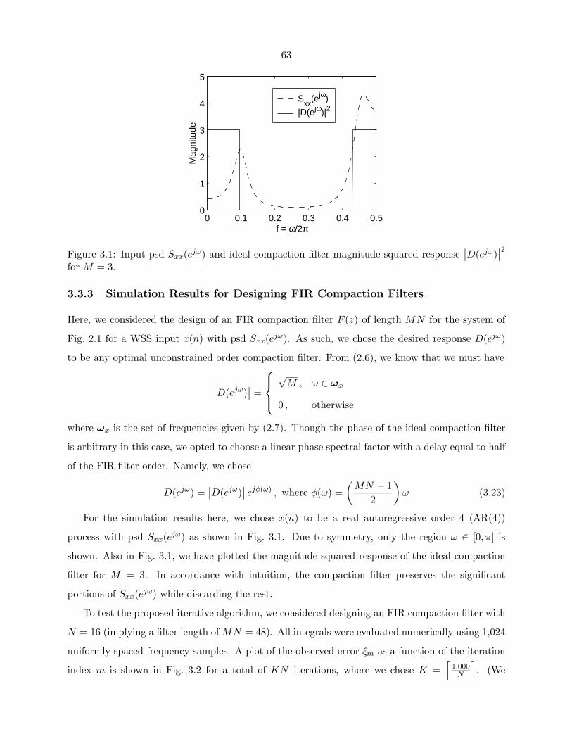
63

0 0.1 0.2 0.3 0.4 0.50

1

2

3

4

5

f = ω/2π

Mag

nitu

de

Sxx

(ejω)

|D(ejω)| 2

Figure 3.1: Input psd Sxx(ejω) and ideal compaction filter magnitude squared response∣∣D(ejω)

∣∣2for M = 3.

3.3.3 Simulation Results for Designing FIR Compaction Filters

Here, we considered the design of an FIR compaction filter F (z) of length MN for the system of

Fig. 2.1 for a WSS input x(n) with psd Sxx(ejω). As such, we chose the desired response D(ejω)

to be any optimal unconstrained order compaction filter. From (2.6), we know that we must have

∣∣D(ejω)∣∣ =

√

M , ω ∈ ωx

0 , otherwise

where ωx is the set of frequencies given by (2.7). Though the phase of the ideal compaction filter

is arbitrary in this case, we opted to choose a linear phase spectral factor with a delay equal to half

of the FIR filter order. Namely, we chose

D(ejω) =∣∣D(ejω)

∣∣ ejφ(ω) , where φ(ω) =(

MN − 12

)ω (3.23)

For the simulation results here, we chose x(n) to be a real autoregressive order 4 (AR(4))

process with psd Sxx(ejω) as shown in Fig. 3.1. Due to symmetry, only the region ω ∈ [0, π] is

shown. Also in Fig. 3.1, we have plotted the magnitude squared response of the ideal compaction

filter for M = 3. In accordance with intuition, the compaction filter preserves the significant

portions of Sxx(ejω) while discarding the rest.

To test the proposed iterative algorithm, we considered designing an FIR compaction filter with

N = 16 (implying a filter length of MN = 48). All integrals were evaluated numerically using 1,024

uniformly spaced frequency samples. A plot of the observed error ξm as a function of the iteration

index m is shown in Fig. 3.2 for a total of KN iterations, where we chose K =⌈

1,000N

⌉. (We

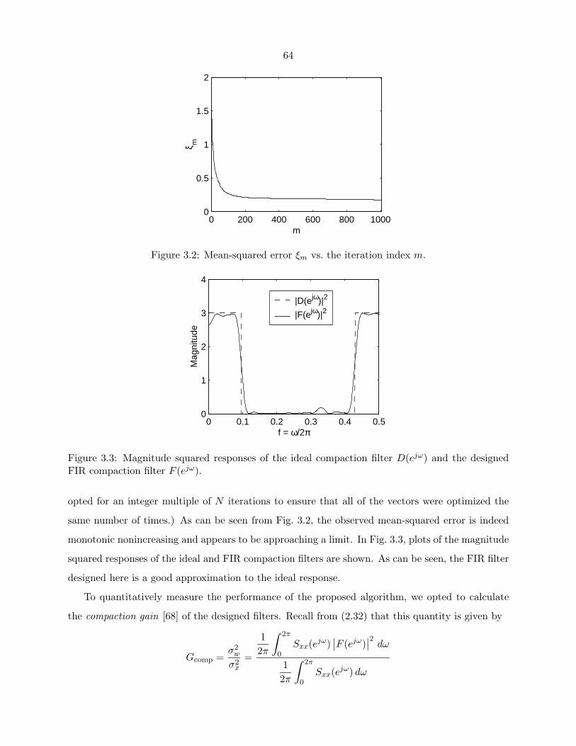
64

0 200 400 600 800 10000

0.5

1

1.5

2

m

ξ m

Figure 3.2: Mean-squared error ξm vs. the iteration index m.

0 0.1 0.2 0.3 0.4 0.50

1

2

3

4

f = ω/2π

Mag

nitu

de

|D(ejω)| 2

|F(ejω)| 2

Figure 3.3: Magnitude squared responses of the ideal compaction filter D(ejω) and the designedFIR compaction filter F (ejω).

opted for an integer multiple of N iterations to ensure that all of the vectors were optimized the

same number of times.) As can be seen from Fig. 3.2, the observed mean-squared error is indeed

monotonic nonincreasing and appears to be approaching a limit. In Fig. 3.3, plots of the magnitude

squared responses of the ideal and FIR compaction filters are shown. As can be seen, the FIR filter

designed here is a good approximation to the ideal response.

To quantitatively measure the performance of the proposed algorithm, we opted to calculate

the compaction gain [68] of the designed filters. Recall from (2.32) that this quantity is given by

Gcomp =σ2

w

σ2x

=

12π

∫ 2π

0Sxx(ejω)

∣∣F (ejω)∣∣2 dω

12π

∫ 2π

0Sxx(ejω) dω

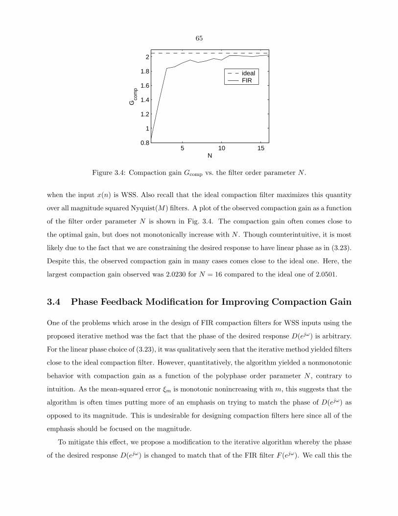
65

5 10 150.8

1

1.2

1.4

1.6

1.8

2

N

Gco

mp

idealFIR

Figure 3.4: Compaction gain Gcomp vs. the filter order parameter N .

when the input x(n) is WSS. Also recall that the ideal compaction filter maximizes this quantity

over all magnitude squared Nyquist(M) filters. A plot of the observed compaction gain as a function

of the filter order parameter N is shown in Fig. 3.4. The compaction gain often comes close to

the optimal gain, but does not monotonically increase with N . Though counterintuitive, it is most

likely due to the fact that we are constraining the desired response to have linear phase as in (3.23).

Despite this, the observed compaction gain in many cases comes close to the ideal one. Here, the

largest compaction gain observed was 2.0230 for N = 16 compared to the ideal one of 2.0501.

3.4 Phase Feedback Modification for Improving Compaction Gain

One of the problems which arose in the design of FIR compaction filters for WSS inputs using the

proposed iterative method was the fact that the phase of the desired response D(ejω) is arbitrary.

For the linear phase choice of (3.23), it was qualitatively seen that the iterative method yielded filters

close to the ideal compaction filter. However, quantitatively, the algorithm yielded a nonmonotonic

behavior with compaction gain as a function of the polyphase order parameter N , contrary to

intuition. As the mean-squared error ξm is monotonic nonincreasing with m, this suggests that the

algorithm is often times putting more of an emphasis on trying to match the phase of D(ejω) as

opposed to its magnitude. This is undesirable for designing compaction filters here since all of the

emphasis should be focused on the magnitude.

To mitigate this effect, we propose a modification to the iterative algorithm whereby the phase

of the desired response D(ejω) is changed to match that of the FIR filter F (ejω). We call this the

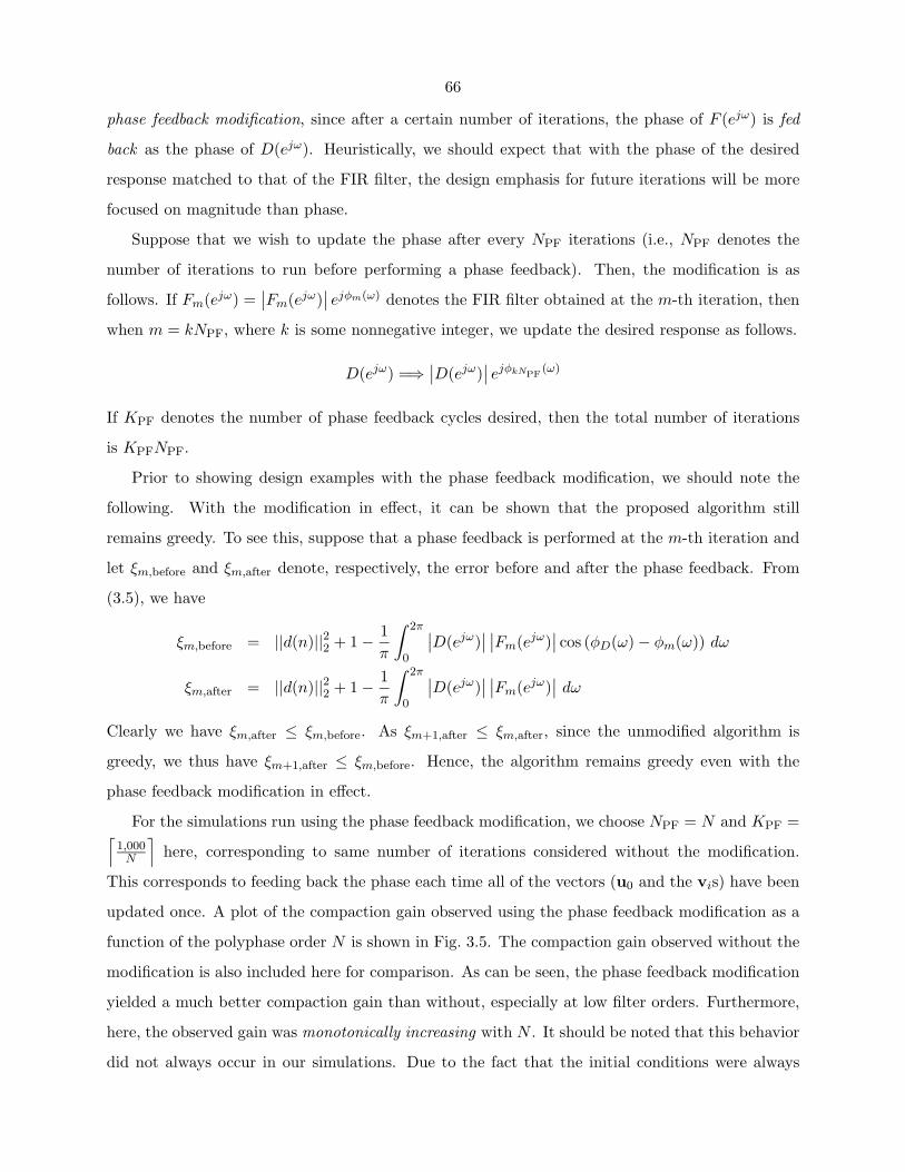
66

phase feedback modification, since after a certain number of iterations, the phase of F (ejω) is fed

back as the phase of D(ejω). Heuristically, we should expect that with the phase of the desired

response matched to that of the FIR filter, the design emphasis for future iterations will be more

focused on magnitude than phase.

Suppose that we wish to update the phase after every NPF iterations (i.e., NPF denotes the

number of iterations to run before performing a phase feedback). Then, the modification is as

follows. If Fm(ejω) =∣∣Fm(ejω)

∣∣ ejφm(ω) denotes the FIR filter obtained at the m-th iteration, then

when m = kNPF, where k is some nonnegative integer, we update the desired response as follows.

D(ejω) =⇒ ∣∣D(ejω)∣∣ ejφkNPF

(ω)

If KPF denotes the number of phase feedback cycles desired, then the total number of iterations

is KPFNPF.

Prior to showing design examples with the phase feedback modification, we should note the

following. With the modification in effect, it can be shown that the proposed algorithm still

remains greedy. To see this, suppose that a phase feedback is performed at the m-th iteration and

let ξm,before and ξm,after denote, respectively, the error before and after the phase feedback. From

(3.5), we have

ξm,before = ||d(n)||22 + 1 − 1π

∫ 2π

0

∣∣D(ejω)∣∣ ∣∣Fm(ejω)

∣∣ cos (φD(ω) − φm(ω)) dω

ξm,after = ||d(n)||22 + 1 − 1π

∫ 2π

0

∣∣D(ejω)∣∣ ∣∣Fm(ejω)

∣∣ dω

Clearly we have ξm,after ≤ ξm,before. As ξm+1,after ≤ ξm,after, since the unmodified algorithm is

greedy, we thus have ξm+1,after ≤ ξm,before. Hence, the algorithm remains greedy even with the

phase feedback modification in effect.

For the simulations run using the phase feedback modification, we choose NPF = N and KPF =⌈1,000

N

⌉here, corresponding to same number of iterations considered without the modification.

This corresponds to feeding back the phase each time all of the vectors (u0 and the vis) have been

updated once. A plot of the compaction gain observed using the phase feedback modification as a

function of the polyphase order N is shown in Fig. 3.5. The compaction gain observed without the

modification is also included here for comparison. As can be seen, the phase feedback modification

yielded a much better compaction gain than without, especially at low filter orders. Furthermore,

here, the observed gain was monotonically increasing with N . It should be noted that this behavior

did not always occur in our simulations. Due to the fact that the initial conditions were always

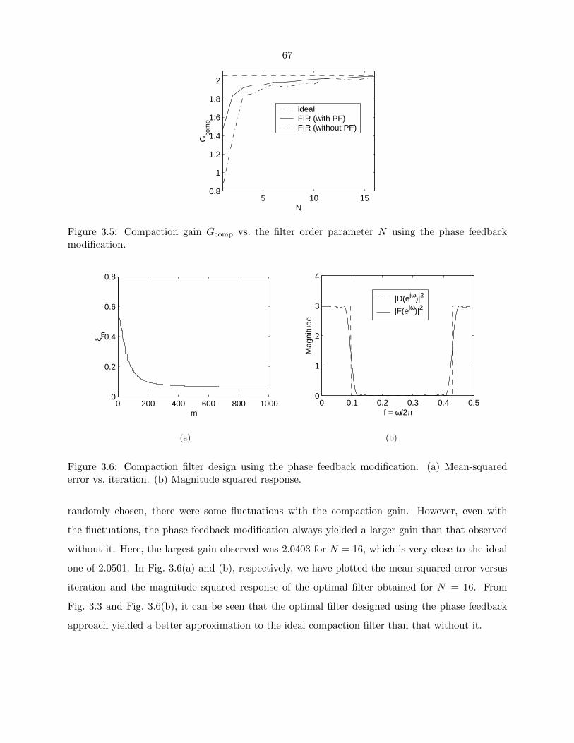
67

5 10 150.8

1

1.2

1.4

1.6

1.8

2

NG

com

p

idealFIR (with PF)FIR (without PF)

Figure 3.5: Compaction gain Gcomp vs. the filter order parameter N using the phase feedbackmodification.

0 200 400 600 800 10000

0.2

0.4

0.6

0.8

m

ξ m

(a)

0 0.1 0.2 0.3 0.4 0.50

1

2

3

4

f = ω/2π

Mag

nitu

de|D(ejω)|

2

|F(ejω)| 2

(b)

Figure 3.6: Compaction filter design using the phase feedback modification. (a) Mean-squarederror vs. iteration. (b) Magnitude squared response.

randomly chosen, there were some fluctuations with the compaction gain. However, even with

the fluctuations, the phase feedback modification always yielded a larger gain than that observed

without it. Here, the largest gain observed was 2.0403 for N = 16, which is very close to the ideal

one of 2.0501. In Fig. 3.6(a) and (b), respectively, we have plotted the mean-squared error versus

iteration and the magnitude squared response of the optimal filter obtained for N = 16. From

Fig. 3.3 and Fig. 3.6(b), it can be seen that the optimal filter designed using the phase feedback

approach yielded a better approximation to the ideal compaction filter than that without it.

68

� �

�

�

↓ M

↓ M

↓ M

�z

�z

�z

�

�

�

F(z)

M × M

�

�

�

x(n)w0(n)

w1(n)

wM−1(n)

x(n)

� �

�

�

F(z)

M × M

�

�

�

z−1

z−1

z−1

�↑ M

↑ M

↑ M

x(n)

x(n)

�

Figure 3.7: Uniform M -channel maximally decimated PU filter bank.

3.5 Design of Signal-Adapted FIR PU Filter Banks

Using a Multiresolution Criterion

In this section, we focus on the PU filter bank shown in Fig. 3.7 in which the M × M synthesis

polyphase matrix F(z) satisfies F(z)F(z) = I and the synthesis filters are given by [67][F0(z) F1(z) · · · FM−1(z)

]= a(z)F

(zM

)(3.24)

Note that this filter bank is just a special case of the system shown in Fig. 1.13. In order to mimic

the behavior of the infinite-order PCFB for the case where F(z) is FIR, we will opt to design F(z)

according to the following multiresolution optimality criterion originally considered by Moulin and

Mıhcak [37].

Multiresolution Optimality Criterion (MOC):

1. Maximize σ2w0

subject to[F0(z)F0(z)

]↓M

= 1 (Compaction Filter Problem)

2. For i = 1, 2, . . . , M − 1, successively maximize σ2wi

subject to[Fi(z)Fi(z)

]↓M

= 1 (Nyquist(M) Criterion)[Fk(z)Fi(z)

]↓M

= 0 ∀ 0 ≤ k ≤ i − 1 (Orthogonality Criterion)

As can be seen, the MOC consists of optimizing the filters one at a time starting with the

design of the compaction filter. At each stage, the next filter is chosen to maximize its subband

variance subject to the remaining degrees of freedom dictated by the PU constraint and the other

filters already designed. A multiresolution optimal filter bank is also said to be optimal in terms of

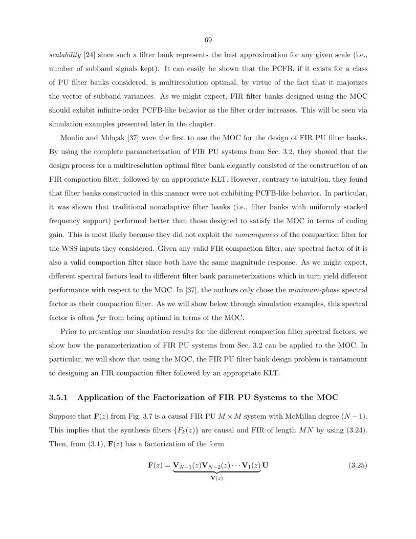
69

scalability [24] since such a filter bank represents the best approximation for any given scale (i.e.,

number of subband signals kept). It can easily be shown that the PCFB, if it exists for a class

of PU filter banks considered, is multiresolution optimal, by virtue of the fact that it majorizes

the vector of subband variances. As we might expect, FIR filter banks designed using the MOC

should exhibit infinite-order PCFB-like behavior as the filter order increases. This will be seen via

simulation examples presented later in the chapter.

Moulin and Mıhcak [37] were the first to use the MOC for the design of FIR PU filter banks.

By using the complete parameterization of FIR PU systems from Sec. 3.2, they showed that the

design process for a multiresolution optimal filter bank elegantly consisted of the construction of an

FIR compaction filter, followed by an appropriate KLT. However, contrary to intuition, they found

that filter banks constructed in this manner were not exhibiting PCFB-like behavior. In particular,

it was shown that traditional nonadaptive filter banks (i.e., filter banks with uniformly stacked

frequency support) performed better than those designed to satisfy the MOC in terms of coding

gain. This is most likely because they did not exploit the nonuniquness of the compaction filter for

the WSS inputs they considered. Given any valid FIR compaction filter, any spectral factor of it is

also a valid compaction filter since both have the same magnitude response. As we might expect,

different spectral factors lead to different filter bank parameterizations which in turn yield different

performance with respect to the MOC. In [37], the authors only chose the minimum-phase spectral

factor as their compaction filter. As we will show below through simulation examples, this spectral

factor is often far from being optimal in terms of the MOC.

Prior to presenting our simulation results for the different compaction filter spectral factors, we

show how the parameterization of FIR PU systems from Sec. 3.2 can be applied to the MOC. In

particular, we will show that using the MOC, the FIR PU filter bank design problem is tantamount

to designing an FIR compaction filter followed by an appropriate KLT.

3.5.1 Application of the Factorization of FIR PU Systems to the MOC

Suppose that F(z) from Fig. 3.7 is a causal FIR PU M ×M system with McMillan degree (N − 1).

This implies that the synthesis filters {Fk(z)} are causal and FIR of length MN by using (3.24).

Then, from (3.1), F(z) has a factorization of the form

F(z) = VN−1(z)VN−2(z) · · ·V1(z)︸ ︷︷ ︸V(z)

U (3.25)

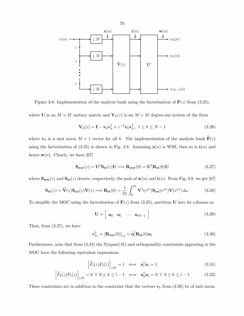
70

� �

�

�

↓ M

↓ M

↓ M

�z

�z

�z

�

�

�

V(z)

�

�

�

U†

�

�

�

x(n) w0(n)

w1(n)

wM−1(n)

x(n)

�

t(n)

�

w(n)

�

Figure 3.8: Implementation of the analysis bank using the factorization of F(z) from (3.25).

where U is an M × M unitary matrix and Vk(z) is an M × M degree-one system of the form

Vk(z) = I − vkv†k + z−1vkv

†k , 1 ≤ k ≤ N − 1 (3.26)

where vk is a unit norm M × 1 vector for all k. The implementation of the analysis bank F(z)

using the factorization of (3.25) is shown in Fig. 3.8. Assuming x(n) is WSS, then so is t(n) and

hence w(n). Clearly, we have [67]

Sww(z) = U†Stt(z)U =⇒ Rww(0) = U†Rtt(0)U (3.27)

where Sww(z) and Stt(z) denote, respectively, the psds of w(n) and t(n). From Fig. 3.8, we get [67]

Stt(z) = V(z)Sxx(z)V(z) =⇒ Rtt(0) =12π

∫ 2π

0V†(ejω)Sxx(ejω)V(ejω) dω (3.28)

To simplify the MOC using the factorization of F(z) from (3.25), partition U into its columns as

U =[

u0 u1 · · · uM−1

](3.29)

Then, from (3.27), we have

σ2wi

= [Rww(0)]i,i = u†iRtt(0)ui (3.30)

Furthermore, note that from (3.24) the Nyquist(M) and orthogonality constraints appearing in the

MOC have the following equivalent expressions.[Fi(z)Fi(z)

]↓M

= 1 ⇐⇒ u†iui = 1 (3.31)[

Fk(z)Fi(z)]↓M

= 0 ∀ 0 ≤ k ≤ i − 1 ⇐⇒ u†kui = 0 ∀ 0 ≤ k ≤ i − 1 (3.32)

These constraints are in addition to the constraint that the vectors vk from (3.26) be of unit norm.

71

Recall that Step 1 of the MOC requires the computation of a compaction filter. Suppose that

a causal FIR compaction filter F0(z) of length MN has already been designed using either the

proposed iterative algorithm or any of the methods described in Section 2.2.2. Substituting (3.25)

and (3.29) in (3.24), it follows that we know the value of

F0(z) = a(z)V(zM

)u0︸ ︷︷ ︸

f0(zM )

(3.33)

where f0(z) = V(z)u0 is an M × 1 causal FIR PU vector system of degree (N − 1) consisting of

Type I polyphase components of F0(z). As f0(z) is a vector system, it follows from Sec. 3.2 that

the diadic forms present in V(z), namely, the quantities vkv†k for 1 ≤ k ≤ N − 1, are unique.

Hence, the matrix V(z) itself is unique. Thus, a given compaction filter F0(z) corresponds to a

unique V(z). It should be noted here that this uniqueness holds iff F0(z) is a nondegenerate causal

FIR filter of length MN , i.e., the length of F0(z) can not be less than MN . In all practical cases,

however, including the FIR compaction filters designed here, this is never a problem since the filters

are always nondegenerate.

To summarize, once a nontrivial FIR compaction filter F0(z) has been designed, we know the

unique value of the matrix V(z) appearing in Fig. 3.8. Hence, the second order statistics of the

process t(n) from Fig. 3.8 are known, namely, the autocorrelation sequence Rtt(k).

It should also be noted that with F0(z) given, we also know the first column u0 of the matrix

U from (3.29). By Rayleigh’s principle [22], it follows that u0 must be a unit norm eigenvector

corresponding to the largest eigenvalue of the matrix Rtt(0) given by (3.27) and (3.28). To see this,

note that with Rtt(0) uniquely determined, using (3.30) and (3.31), Step 1 of the MOC becomes

Maximize σ2w0

= u†0Rtt(0)u0 subject to u†

0u0 = 1.

which is precisely the problem statement in Rayleigh’s principle [22].

To determine the other columns u1,u2, . . . ,uM−1 of the matrix U from (3.29), note that with

Rtt(0) uniquely determined, from (3.30), (3.31), and (3.32), Step 2 of the MOC becomes

Maximize σ2wi

= u†iRtt(0)ui subject to u†

iui = 1 and u†kui = 0 ∀ 0 ≤ k ≤ i − 1.

This is done successively for i = 1, 2, . . . , M − 1. As such, the vectors u1,u2, . . . ,uM−1 are found

sequentially beginning with u1 and ending with uM−1. By an extension of Rayleigh’s principle [22],

it follows that u1 must be a unit norm eigenvector corresponding to the second largest eigenvalue

of Rtt(0). Similarly, by extension of Rayleigh’s principle, ui must be a unit norm eigenvector

72

corresponding to the i-th largest eigenvalue of Rtt(0) for all i. In other words, the optimal matrix

U from (3.29) is the unitary matrix which diagonalizes Rtt(0). Hence, the optimal U is a KLT for

the process t(n) from Fig. 3.8. Furthermore, the subband variances σ2wi

are simply the eigenvalues

of Rtt(0).

In conclusion, designing an FIR PU filter bank using the MOC consists of computing an optimal

FIR compaction filter followed by an appropriate KLT. A summary of this design algorithm is given

below.

3.5.2 Algorithm for the Design of FIR PU Multiresolution Optimal

Filter Banks

1. Design an optimal causal FIR compaction filter F0(z) of length MN . Identify the M×1 causal

PU vector f0(z) of degree (N − 1) from (3.33) via a Type I M -fold polyphase decomposition.

2. Find the unique Vk(z) from (3.26) corresponding to f0(z) as follows. Define the M ×1 vector

system Pk(z) from k = N − 1, N − 2, . . . , 1 as

PN−1(z) � f0(z) , Pk−1(z) � Vk(z)Pk(z) (3.34)

Then, in order for Pk(z) to be a polynomial in z−1 of degree k of the form

Pk(z) =k∑

n=0

pk(n)z−n (3.35)

we must have

vk = ckpk(k)

||pk(k)|| for some ck with |ck| = 1 =⇒ vkv†k =

pk(k)p†k(k)

||pk(k)||2 =pk(k)p†

k(k)

p†k(k)pk(k)

(3.36)

Hence, the diadic terms vkv†k appearing in Vk(z) from (3.26) are found recursively starting

from k = N − 1 and ending at k = 1 using (3.34), (3.35), and (3.36) successively.

3. Compute V(z) = VN−1(z)VN−2(z) · · ·V1(z). Then calculate Rtt(0) using (3.28).

4. Choose U to be the KLT of t(n), i.e., the unitary matrix which diagonalizes Rtt(0).

5. Compute the synthesis polyphase matrix F(z) using F(z) = V(z)U.

73

2 4 6 8 10

1.2

1.3

1.4

1.5

1.6

1.7

N

Cod

ing

Gai

n

PCFBFIR PU (opt)FIR PU (min−φ)KLT

Figure 3.9: Observed coding gain Gcode as a function of the synthesis polyphase order N .

3.6 Simulation Results for MOC Designed FIR PU Filter Banks

3.6.1 Coding Gain Results

Suppose that the input x(n) to the PU filter bank of Fig. 3.7 is the real AR(4) process considered

in Sec. 3.3.3, whose psd Sxx(ejω) is shown in Fig. 3.1. Here, we considered the design of an M = 3

channel system. For each filter bank designed, the filters designed in Sec. 3.4 using the proposed

iterative algorithm with the phase feedback modification were used as the optimum FIR compaction

filter required for multiresolution optimality. The synthesis polyphase matrix order N was varied

from 1 to 11 in order to see the behavior of the filter banks designed. For each N , the filter banks

corresponding to all compaction filter spectral factors were computed and the one judged to be

optimal was the one which yielded the largest coding gain. (See Chapter 5 for more on coding

gain.) Assuming optimal bit allocation, the coding gain is given by [67]

Gcode =

1M

M−1∑i=0

σ2wi(

M−1∏i=0

σ2wi

) 1M

In this case, the coding gain is simply the arithmetic mean/geometric mean (AM/GM) ratio of the

subband variances. Due to the subband variance majorization property of the PCFB, it can be

shown that the PCFB, if it exists for a class of filter banks under consideration, maximizes this

quantity [1]. Hence, the coding gain is lower bounded by unity (because of the AM/GM inequality

[67]) and upper bounded by the gain produced by the PCFB.

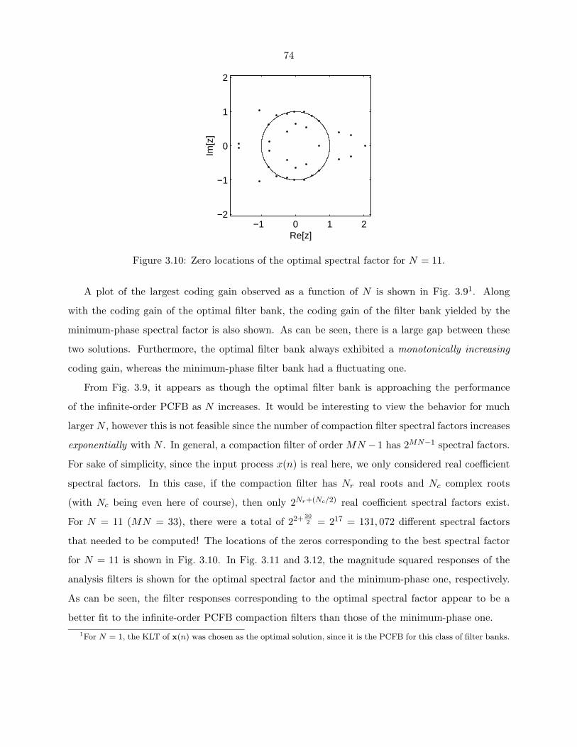
74

−1 0 1 2−2

−1

0

1

2

Re[z]

Im[z

]

Figure 3.10: Zero locations of the optimal spectral factor for N = 11.

A plot of the largest coding gain observed as a function of N is shown in Fig. 3.91. Along

with the coding gain of the optimal filter bank, the coding gain of the filter bank yielded by the

minimum-phase spectral factor is also shown. As can be seen, there is a large gap between these

two solutions. Furthermore, the optimal filter bank always exhibited a monotonically increasing

coding gain, whereas the minimum-phase filter bank had a fluctuating one.

From Fig. 3.9, it appears as though the optimal filter bank is approaching the performance

of the infinite-order PCFB as N increases. It would be interesting to view the behavior for much

larger N , however this is not feasible since the number of compaction filter spectral factors increases

exponentially with N . In general, a compaction filter of order MN − 1 has 2MN−1 spectral factors.

For sake of simplicity, since the input process x(n) is real here, we only considered real coefficient

spectral factors. In this case, if the compaction filter has Nr real roots and Nc complex roots

(with Nc being even here of course), then only 2Nr+(Nc/2) real coefficient spectral factors exist.

For N = 11 (MN = 33), there were a total of 22+ 302 = 217 = 131, 072 different spectral factors

that needed to be computed! The locations of the zeros corresponding to the best spectral factor

for N = 11 is shown in Fig. 3.10. In Fig. 3.11 and 3.12, the magnitude squared responses of the

analysis filters is shown for the optimal spectral factor and the minimum-phase one, respectively.

As can be seen, the filter responses corresponding to the optimal spectral factor appear to be a

better fit to the infinite-order PCFB compaction filters than those of the minimum-phase one.1For N = 1, the KLT of x(n) was chosen as the optimal solution, since it is the PCFB for this class of filter banks.

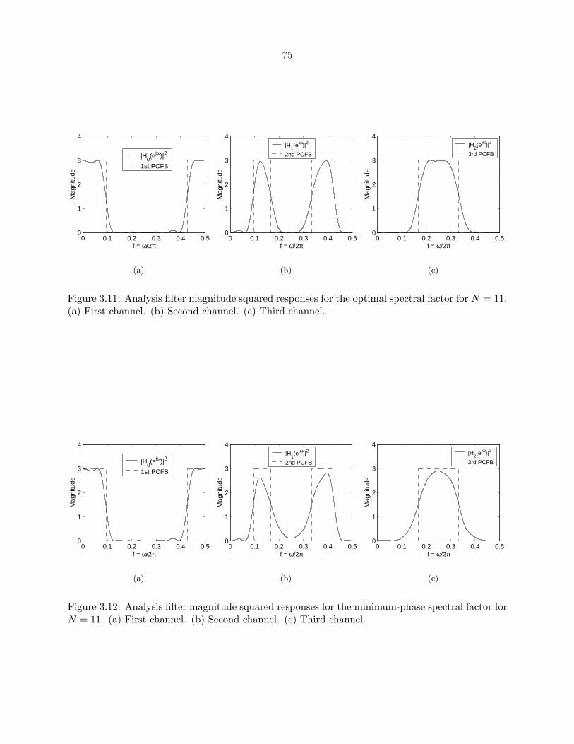
75

0 0.1 0.2 0.3 0.4 0.50

1

2

3

4

f = ω/2π

Mag

nitu

de

|H0(ejω)|2

1st PCFB

(a)

0 0.1 0.2 0.3 0.4 0.50

1

2

3

4

f = ω/2π

Mag

nitu

de

|H1(ejω)|2

2nd PCFB

(b)

0 0.1 0.2 0.3 0.4 0.50

1

2

3

4

f = ω/2π

Mag

nitu

de

|H2(ejω)|2

3rd PCFB

(c)

Figure 3.11: Analysis filter magnitude squared responses for the optimal spectral factor for N = 11.(a) First channel. (b) Second channel. (c) Third channel.

0 0.1 0.2 0.3 0.4 0.50

1

2

3

4

f = ω/2π

Mag

nitu

de

|H0(ejω)|2

1st PCFB

(a)

0 0.1 0.2 0.3 0.4 0.50

1

2

3

4

f = ω/2π

Mag

nitu

de

|H1(ejω)|2

2nd PCFB

(b)

0 0.1 0.2 0.3 0.4 0.50

1

2

3

4

f = ω/2π

Mag

nitu

de

|H2(ejω)|2

3rd PCFB

(c)

Figure 3.12: Analysis filter magnitude squared responses for the minimum-phase spectral factor forN = 11. (a) First channel. (b) Second channel. (c) Third channel.

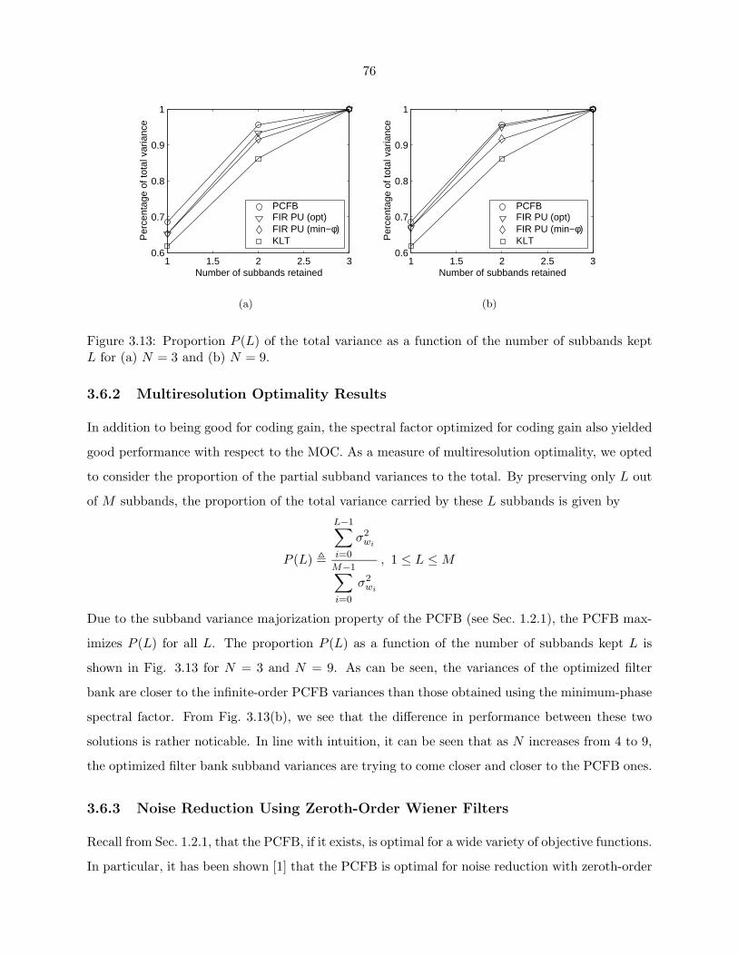
76

1 1.5 2 2.5 30.6

0.7

0.8

0.9

1

Number of subbands retained

Per

cent

age

of to

tal v

aria

nce

PCFBFIR PU (opt)FIR PU (min−φ)KLT

(a)

1 1.5 2 2.5 30.6

0.7

0.8

0.9

1

Number of subbands retained

Per

cent

age

of to

tal v

aria

nce

PCFBFIR PU (opt)FIR PU (min−φ)KLT

(b)

Figure 3.13: Proportion P (L) of the total variance as a function of the number of subbands keptL for (a) N = 3 and (b) N = 9.

3.6.2 Multiresolution Optimality Results

In addition to being good for coding gain, the spectral factor optimized for coding gain also yielded

good performance with respect to the MOC. As a measure of multiresolution optimality, we opted

to consider the proportion of the partial subband variances to the total. By preserving only L out

of M subbands, the proportion of the total variance carried by these L subbands is given by

P (L) �

L−1∑i=0

σ2wi

M−1∑i=0

σ2wi

, 1 ≤ L ≤ M

Due to the subband variance majorization property of the PCFB (see Sec. 1.2.1), the PCFB max-

imizes P (L) for all L. The proportion P (L) as a function of the number of subbands kept L is

shown in Fig. 3.13 for N = 3 and N = 9. As can be seen, the variances of the optimized filter

bank are closer to the infinite-order PCFB variances than those obtained using the minimum-phase

spectral factor. From Fig. 3.13(b), we see that the difference in performance between these two

solutions is rather noticable. In line with intuition, it can be seen that as N increases from 4 to 9,

the optimized filter bank subband variances are trying to come closer and closer to the PCFB ones.

3.6.3 Noise Reduction Using Zeroth-Order Wiener Filters

Recall from Sec. 1.2.1, that the PCFB, if it exists, is optimal for a wide variety of objective functions.

In particular, it has been shown [1] that the PCFB is optimal for noise reduction with zeroth-order

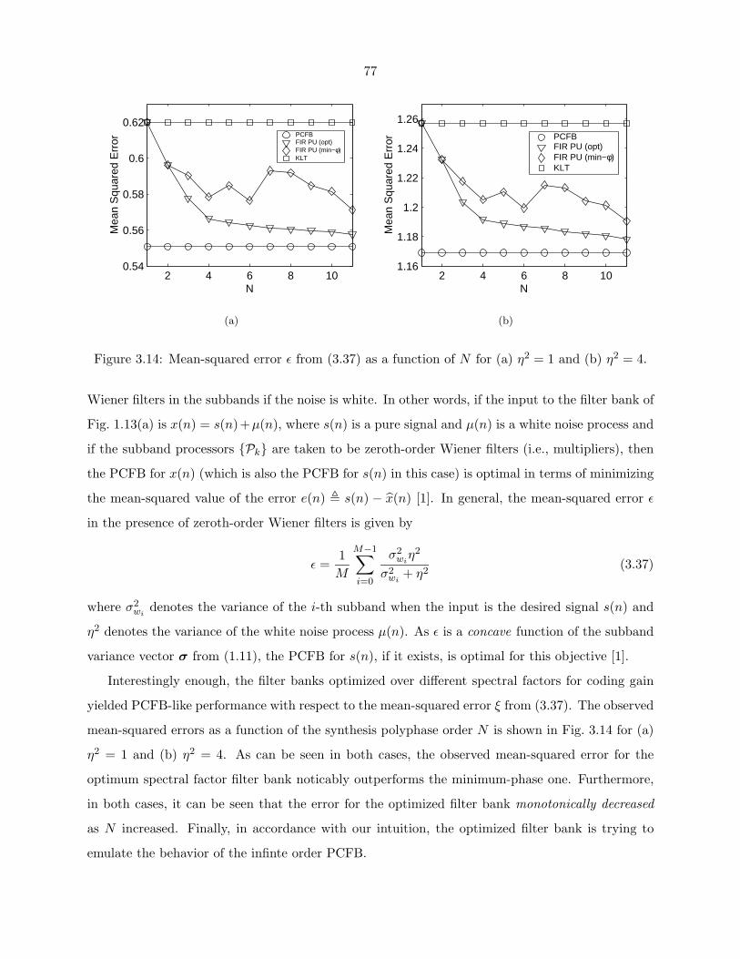
77

2 4 6 8 100.54

0.56

0.58

0.6

0.62

N

Mea

n S

quar

ed E

rror

PCFBFIR PU (opt)FIR PU (min−φ)KLT

(a)

2 4 6 8 101.16

1.18

1.2

1.22

1.24

1.26

N

Mea

n S

quar

ed E

rror PCFB

FIR PU (opt)FIR PU (min−φ)KLT

(b)

Figure 3.14: Mean-squared error ε from (3.37) as a function of N for (a) η2 = 1 and (b) η2 = 4.

Wiener filters in the subbands if the noise is white. In other words, if the input to the filter bank of

Fig. 1.13(a) is x(n) = s(n)+µ(n), where s(n) is a pure signal and µ(n) is a white noise process and

if the subband processors {Pk} are taken to be zeroth-order Wiener filters (i.e., multipliers), then

the PCFB for x(n) (which is also the PCFB for s(n) in this case) is optimal in terms of minimizing

the mean-squared value of the error e(n) � s(n) − x(n) [1]. In general, the mean-squared error ε

in the presence of zeroth-order Wiener filters is given by

ε =1M

M−1∑i=0

σ2wi

η2

σ2wi

+ η2(3.37)

where σ2wi

denotes the variance of the i-th subband when the input is the desired signal s(n) and

η2 denotes the variance of the white noise process µ(n). As ε is a concave function of the subband

variance vector σ from (1.11), the PCFB for s(n), if it exists, is optimal for this objective [1].

Interestingly enough, the filter banks optimized over different spectral factors for coding gain

yielded PCFB-like performance with respect to the mean-squared error ξ from (3.37). The observed

mean-squared errors as a function of the synthesis polyphase order N is shown in Fig. 3.14 for (a)

η2 = 1 and (b) η2 = 4. As can be seen in both cases, the observed mean-squared error for the

optimum spectral factor filter bank noticably outperforms the minimum-phase one. Furthermore,

in both cases, it can be seen that the error for the optimized filter bank monotonically decreased

as N increased. Finally, in accordance with our intuition, the optimized filter bank is trying to

emulate the behavior of the infinte order PCFB.

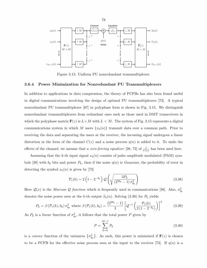
78

� �

�

�

↓ M

↓ M

↓ M

�z

�z

�z

�

�

�

F(z)

M × M

�

�

�

x0(n)

x1(n)

xM−1(n)

�

�

�

�

�

�

F(z)

M × M

�

�

�

z−1

z−1

z−1

�

Channel

C(z) �

η(n)

Noise

�

Equalizer

1C(z)↑ M

↑ M

↑ M

x0(n)

x1(n)

xM−1(n)

Figure 3.15: Uniform PU nonredundant transmultiplexer.

3.6.4 Power Minimization for Nonredundant PU Transmultiplexers

In addition to applications in data compression, the theory of PCFBs has also been found useful

in digital communications involving the design of optimal PU transmultiplexers [73]. A typical

nonredundant PU transmultiplexer [67] in polyphase form is shown in Fig. 3.15. We distinguish

nonredundant transmultiplexers from redundant ones such as those used in DMT transceivers in

which the polyphase matrix F(z) is L×M with L < M . The system of Fig. 3.15 represents a digital

communications system in which M users {xk(n)} transmit data over a common path. Prior to

receiving the data and separating the users at the receiver, the incoming signal undergoes a linear

distortion in the form of the channel C(z) and a noise process η(n) is added to it. To undo the

effects of the channel, we assume that a zero-forcing equalizer [38, 73] of 1C(z) has been used here.

Assuming that the k-th input signal xk(n) consists of pulse amplitude modulated (PAM) sym-

bols [38] with bk bits and power Pk, then if the noise η(n) is Gaussian, the probability of error in

detecting the symbol xk(n) is given by [73]

Pe(k) = 2(1 − 2−bk

)Q(√

3Pk

(22bk − 1) σ2qk

)(3.38)

Here Q(x) is the Marcum Q function which is frequently used in communications [38]. Also, σ2qk

denotes the noise power seen at the k-th output xk(n). Solving (3.38) for Pk yields

Pk = β (Pe(k), bk)σ2qk

where β (Pe(k), bk) =

(22bk − 1

)3

[Q−1

( Pe(k)2 (1 − 2−bk)

)]2

(3.39)

As Pk is a linear function of σ2qk

, it follows that the total power P given by

P =M−1∑k=0

Pk (3.40)

is a convex function of the variances{σ2

qk

}. As such, this power is minimized if F(z) is chosen

to be a PCFB for the effective noise process seen at the input to the receiver [73]. If η(n) is a

79

2 4 6 8 10

2

2.5

3

3.5

4

4.5

5

x 104

N

Tot

al R

equi

red

Pow

er PCFBFIR PU (opt)FIR PU (min−φ)KLT

Figure 3.16: Total required power P from (3.40) as a function of N .

WSS process with psd Sηη(ejω), then the effective noise seen at the receiver input is WSS with psdSηη(ejω)

|C(ejω)|2 . Hence, the total power P from (3.40) is minimized if F(z) is a PCFB for the psd Sηη(ejω)

|C(ejω)|2 .

As an example, suppose that the desired probability of error is Pe(k) = 10−9 for all k. Also,

suppose that b0 = 2, b1 = 4, and b2 = 6. (This is a not an optimal bit allocation [73] and is only

chosen as such for simplicity.) Finally, suppose that the effective noise psd Sηη(ejω)

|C(ejω)|2 is simply the

psd Sxx(ejω) shown in Fig. 3.1. Then, the observed required powers as a function of the synthesis

polyphase order N is shown in Fig. 3.16. As can be seen, the optimal spectral factor not only

outperforms the minimum-phase one, but also monotonically decreases with N . The optimized

filter bank appears to be approaching the performance of the infinite-order, in line with intuition.

3.7 Concluding Remarks

In this chapter, we presented a method for the design of FIR compaction filters based on the

complete parameterization of FIR PU systems shown in Sec. 3.2. Using this same characterization,

we constructed FIR PU signal-adapted filter banks based on the MOC of Sec. 3.5 using only these

filters. Through simulations provided, we showed examples of FIR PU filter banks exhibiting an

increasingly PCFB-like behavior as the filter order increased. This behavior has not previously been

seen in the literature. However, this came at the expense of an exponential increase in complexity on

account of the nonuniqueness of the FIR compaction filter. In the next chapter, we present a direct

method for the design of signal-adapted FIR PU filter banks that avoids the problems caused by

the ambiguity of the compaction filter. Furthermore, with this new method, the above-mentioned

PCFB-like behavior continues to hold true.

80

Chapter 4

Direct FIR PU Approximationof the PCFB

Though the signal-adapted filter bank design algorithm of the previous chapter was shown to yield

FIR PU filter banks that behaved more like the infinite-order PCFB as the filter order increased,

it was shown to suffer from one major drawback. In particular, it was shown that the inherent

nonuniqueness of the FIR compaction filter in terms of its spectral factors added an exponential

increase in computational complexity, since each spectral factor needed to be tested for its perfor-

mance. This suggests that the FIR compaction filter problem is perhaps not well suited for the

design of complete signal-adapted filter banks. To avoid this dilemma, in this chapter, we present

a signal-adapted filter bank design algorithm in which all of the filters are found simultaneously.

In particular, using the complete parameterization of FIR PU systems given in [75, 67], an

iterative algorithm is proposed to approximate, in a weighted least-squares sense, any MIMO desired

response by an FIR PU MIMO approximant. This is both a generalization of and departure from

the FIR compaction filter design method from the previous chapter in the sense that it applies to

general MIMO systems and allows for the incorporation of a weight function. As with the previous

method, at each iteration, one set of parameters in the characterization of the FIR PU system

is globally optimized assuming all other parameters to be fixed. Because of this, as before, the

resulting algorithm is greedy and so the error is guaranteed to be monotonic nonincreasing with

iteration.

When the desired response is the synthesis polyphase matrix of an infinite-order PCFB, the

algorithm can be used for the design of the entire FIR PU synthesis bank. As the desired response in

this case suffers from a phase-type ambiguity, which we define here, a modification to the algorithm

is proposed in which the phase of the FIR approximant is cleverly fed back to the desired response.

81

With this phase feedback modification, which is a generalization of the one proposed in the previous

chapter, the iterative algorithm not only still remains greedy, but also yields a better magnitude-type

fit to the desired response. Simulation results provided here show that, with the phase feedback

modification in effect, the FIR PU filter banks designed exhibit an increasingly PCFB-like behavior

as the filter order increases. In particular, in terms of objectives such as coding gain, denoising

using zeroth-order Wiener filters in the subbands, and power minimization for nonredundant PU

transmultiplexers, the FIR PU filter banks designed monotonically approached the performance

of the infinite-order PCFB as the filter order increased. As with the method presented in the

previous chapter, this serves to bridge the gap between the zeroth-order KLT and infinite-order

PCFB. However, unlike the previous method, there is no additional exponential overhead as we

are no longer plagued by the nonuniqueness of the FIR compaction filter as before. In fact, the

algorithm proposed here is only nominally more computationally complex than the compaction

filter design algorithm of the previous chapter.

As we are able to incorporate a weight function in the design algorithm, in addition to being

useful for the design of signal-adapted filter banks, the algorithm can also be used for the FIR PU

interpolation problem mentioned in Sec. 1.3. Though this problem is still open, the iterative greedy

algorithm proposed here can always be used to approximate a desired interpolant. Furthermore, for

cases in which an interpolant is known to exist, the algorithm can be used to find the interpolant,

as shown through simulations presented. Thus, the main contribution of the proposed algorithm

here is a numerical approach to solve a theoretically intractable problem.

The content of this chapter is drawn from [50].

4.1 Outline

In Sec. 4.2, we analyze the weighted least-squares FIR PU approximation problem. Using the

complete parameterization of FIR PU systems introduced in Sec. 3.2, we show how to obtain the

optimal parameters in Sec. 4.2.1 and 4.2.2. The iterative algorithm for obtaining the FIR PU

approximant is formally introduced in Sec. 4.2.3 and is shown to be greedy there.

In Sec. 4.3, we introduce the phase feedback modification to the iterative algorithm for cases in

which the desired response has a phase-type ambiguity. We begin by formally defining the phase-

type ambiguity in Sec. 4.3.1 and then proceed to derive the phase feedback modification in Sec.

4.3.2. In Sec. 4.3.3, we show that the iterative algorithm continues to be greedy with the phase

82

feedback modification in effect.

Simulation results for the proposed iterative greedy algorithm are presented in Sec. 4.4. In Sec.

4.4.1, we focus on the design of infinite-order PCFB-like FIR PU filter banks. There, the FIR

PU filter banks designed are shown to monotonically behave more and more like the infinite-order

PCFB in terms of several objectives. In Sec. 4.4.2, simulation results are presented for the FIR PU

interpolation problem.

Finally, concluding remarks are made in Sec. 4.5. There, we discuss the bridging of the gap be-

tween the zeroth-order KLT and infinite-order PCFB presented here, which has not been previously

reported in the literature.

4.2 The FIR PU Approximation Problem

Let D(ejω) be any p×r desired response matrix that we wish to approximate with a p×r causal FIR

PU system F(ejω) of McMillan degree (N − 1). Note that we require p ≥ r in order to satisfy the

PU condition F(z)F(z) = Ir. Here, we opt to choose F(ejω) to minimize a weighted mean-squared

Frobenius norm error between D(ejω) and F(ejω) given by

ξ � 12π

∫ 2π

0W (ω)

∣∣∣∣D(ejω) − F(ejω)∣∣∣∣2

Fdω (4.1)

Here, W (ω) is a scalar nonnegative weight function and ||A||F denotes the Frobenius norm of any

matrix A given by ||A||F =√

Tr [A†A] [22]. If we only impose an FIR constraint on F(z), then

the optimal filter coefficients of F(z) can be found in closed form in terms of an appropriate matrix

inverse as shown by Tufts and Francis in 1970 [63]. With the additional PU constraint that we

impose here, however, this problem becomes more complicated as we show.

Expanding (4.1) and using the PU condition F(z)F(z) = Ir on F(z) yields the following.

ξ =12π

∫ 2π

0W (ω)

∣∣∣∣D(ejω)∣∣∣∣2

Fdω +

r

2π

∫ 2π

0W (ω) dω︸ ︷︷ ︸

a

− 12π

∫ 2π

0W (ω) Tr

[D†(ejω)F(ejω) + F†(ejω)D(ejω)

]dω (4.2)

Note that the quantity a in (4.2) is simply a constant and that the only quantity that depends on

the system F(z) is the last term of (4.2). Hence, with the PU constraint in effect, the error ξ is

linear or first-order in F(z). This will greatly simplify the optimization problem as will soon be

shown.

83

To help solve this optimization problem with the PU constraint on F(z), we exploit the complete

parameterization of causal FIR PU systems in terms of Householder-like degree-one building blocks

[75, 67]. In particular, F(z) is a causal FIR PU system of McMillan degree (N − 1) iff it is of the

form

F(z) = V(z)U (4.3)

where V(z) is a p× p PU matrix consisting of (N − 1) degree-one Householder-like building blocks

of the form

V(z) =1∏

i=N−1

Vi(z) , Vi(z) = Ip − viv†i + z−1viv

†i , 1 ≤ i ≤ N − 1 (4.4)

where the vectors vi are unit norm vectors, i.e., v†ivi = 1 for all i. Also, the matrix U is some p× r

unitary matrix, i.e., U†U = Ir.

Though it is difficult to jointly optimize the parameters U and {vk} which minimize ξ from

(4.2), it will be shown that optimizing each parameter separately while holding all other parameters

fixed is very simple. This will lead to the proposed iterative algorithm whereby the parameters are

individually optimized at each iteration.

4.2.1 Optimal Choice of U

Substituting (4.3) into (4.2) yields the following.

ξ = a − 12π

∫ 2π

0W (ω) Tr

[D†(ejω)V(ejω)U + U†V†(ejω)D(ejω)

]dω

= a − Tr[ (

12π

∫ 2π

0W (ω)D†(ejω)V(ejω) dω

)︸ ︷︷ ︸

A†

U]

− Tr[

U†(

12π

∫ 2π

0W (ω)V†(ejω)D(ejω) dω

)︸ ︷︷ ︸

A

](4.5)

= a − 2 Re[Tr[U†A

]]︸ ︷︷ ︸

µ

(4.6)

Note that minimizing ξ from (4.6) is equivalent to maximizing µ. To find the optimal p× r unitary

matrix U which maximizes µ, we must exploit the singular value decomposition (SVD) [22] of A.

Suppose that A has the following SVD.

A = TΣW† (4.7)

84

Here, T and W are, respectively, p × p and r × r unitary matrices. The quantity Σ is a p × r

diagonal matrix of the form

Σ =

Σ0 0ρ×(r−ρ)

0(p−ρ)×ρ 0(p−ρ)×(r−ρ)

(4.8)

where ρ = rank(A) and Σ0 is a diagonal matrix of the singular values of A. In other words, we

have Σ0 = diag (σ0, σ1, . . . , σρ−1) where {σi} are the singular values of A which satisfy σi > 0 for

all 0 ≤ i ≤ ρ − 1. Substituting (4.7) into (4.6) yields the following.

µ = Re[Tr[U†TΣW†

]]= Re

[Tr[ΣW†U†T︸ ︷︷ ︸

G†

] ](4.9)

Note that the p × r matrix G = T†UW is unitary, i.e., G†G = Ir. As such, the components of G

satisfy

Re[[G]k,�

]≤ 1 (4.10)

with equality iff [G]k,q = δ(q−�) and [G]p,� = δ(p−k), since the columns of G form an orthonormal

set of vectors [22]. Using (4.8) in (4.9) yields

µ = Re[Tr[ΣG†

]]= Re

[ρ−1∑i=0

σi [G]∗i,i

]=

ρ−1∑i=0

σi Re[[G]∗i,i

]=

ρ−1∑i=0

σi Re[[G]i,i

](4.11)

In light of (4.10) and the fact that σi > 0 for all i, from (4.11), we have

µ ≤ρ−1∑i=0

σi (4.12)

with equality iff [G]i,q = δ(q − i) and [G]p,i = δ(p − i) for all 0 ≤ i ≤ ρ − 1. Since G is unitary, we

have equality iff

G = Gopt =

Iρ 0ρ×(r−ρ)

0(p−ρ)×ρ G0

(4.13)

where G0 is an arbitrary (p−ρ)× (r−ρ) unitary matrix, i.e., G†0G0 = I(r−ρ). As G = T†UW, we

have U = TGW†, and so the optimum U and corresponding optimal value of ξ is given by (4.12)

and (4.6) to be the following.

Uopt = TGoptW† with Gopt as in (4.13) , ξopt = a − 2

(ρ−1∑i=0

σi

)(4.14)

85

In the special case where ρ = r (i.e., A has full rank), we have

Uopt = T

W†

0(p−r)×r

, ξopt = a − 2

(r−1∑i=0

σi

)

Since the matrices T and W from (4.14) depend on V(z), the choice of U from (4.14) is optimal

for fixed W (ω), D(ejω), and V(z).

4.2.2 Optimal Choice of vk

In order to find the optimal choice of vk assuming that all other parameters are fixed, we must

cleverly extract only those portions of ξ which depend on vk. Similar to what was done for the

iterative method of the previous chapter (see (3.15) and (3.16)), for simplicity, let us define the

following p × p matrices.

Lk(z) �

k+1∏

i=N−1

Vi(z) , 0 ≤ k ≤ N − 2

Ip , k = N − 1

(4.15)

Rk(z) �

Ip , k = 1

1∏i=k−1

Vi(z) , 2 ≤ k ≤ N(4.16)

As before, note that Lk(z) and Rk(z) are, respectively, the left and right neighbors of the matrix

Vk(z) for 1 ≤ k ≤ N −1 appearing in V(z) from (4.4). In other words, the following relation holds

true here.

V(z) = Lk(z)Vk(z)Rk(z) , 1 ≤ k ≤ N − 1 (4.17)

86

Also note that by construction, we have L0(z) = RN (z) = V(z). Substituting (4.17) and (4.4) into

(4.3) and (4.2) yields the following.

ξ = a − 12π

∫ 2π

0W (ω) Tr

[D†(ejω)Lk(ejω)Rk(ejω)U

]dω︸ ︷︷ ︸

c

+12π

∫ 2π

0W (ω) Tr

[D†(ejω)Lk(ejω)

(1 − e−jω

)vkv

†kRk(ejω)U

]dω

− 12π

∫ 2π

0W (ω) Tr

[U†R†

k(ejω)L†

k(ejω)D(ejω)

]dω︸ ︷︷ ︸

c∗

+12π

∫ 2π

0W (ω) Tr

[U†R†

k(ejω)

(1 − ejω

)vkv

†kL†

k(ejω)D(ejω)

]dω (4.18)

= a − 2 Re [c] + v†k

[12π

∫ 2π

0W (ω)

(1 − e−jω

)Rk(ejω)UD†(ejω)Lk(ejω) dω

]︸ ︷︷ ︸

B

vk

+ v†k

[12π

∫ 2π

0W (ω)

(1 − ejω

)L†k(e

jω)D(ejω)U†R†k(e

jω) dω

]︸ ︷︷ ︸

B†

vk (4.19)

= a − 2 Re [c] + v†k

(B + B†

)︸ ︷︷ ︸

Q

vk = a − 2 Re [c] + v†kQvk︸ ︷︷ ︸

ν

(4.20)

Here, the quantity c defined in (4.18) depends on all of the parameters except vk. Hence, to

minimize ξ with respect to vk, we must minimize the quantity ν from (4.20). But note that

ν = v†kQvk is simply a quadratic form corresponding to the Hermitian matrix Q [22]. As vk must

satisfy v†kvk = 1, it follows from Rayleigh’s principle [22] that the optimal vk must be a unit norm

eigenvector corresponding to the smallest eigenvalue of Q. If λmin denotes the smallest eigenvalue

of Q and wmin is any unit norm eigenvector corresponding to λmin, then the optimum choice of vk

and corresponding optimal ξ are given by (4.20) to be the following.

vk,opt = wmin , ξopt = a − 2 Re [c] + λmin (4.21)

Note that since wmin from (4.21) depends on Lk(z), Rk(z), and U, it follows that the choice of vk

from (4.21) is optimal for fixed W (ω), D(ejω), U, and all vi for which i �= k.

In summary, finding the optimal parameters corresponding to the Householder-like factorization

of causal FIR PU systems is simple if the parameters are optimized individually. The process of

updating the individual parameters to their optimal values forms the basis of the proposed iterative

algorithm for solving the FIR PU approximation problem, which we now present.

87

4.2.3 Iterative Greedy Algorithm for Solving the Approximation Problem

Let ξm denote the mean-squared error at the m-th iteration for m ≥ 0. Then, the iterative algorithm

for solving the FIR PU approximation problem is as follows.

Initialization:

1. Generate a random p× r unitary matrix U and (N − 1) p× 1 random unit norm vectors

vi, 1 ≤ i ≤ N − 1.

2. Compute the matrix RN (z) using (4.16).

Iteration: For m ≥ 0, do the following.

1. If m is a multiple of N :

(a) Calculate the optimal U and corresponding ξm using (4.14), (4.7), and (4.5) with

V(z) = RN (z).

(b) Compute L0(z) = V(z) and R1(z) = Ip.

Otherwise, if m ≡ k mod N where 1 ≤ k ≤ N − 1:

(a) From (4.15), update the left matrix as Lk(z) = Lk−1(z)Vk(z).

(b) Calculate the optimal vk and corresponding ξm using (4.21), (4.20), (4.19), and

(4.18).

(c) From (4.16), update the right matrix as Rk+1(z) = Vk(z)Rk(z).

2. Increment m by 1 and return to Step 1.

Note that like the iterative algorithm of the previous chapter (see Sec. 3.3.2), as the iterations

progress, the left matrix is shortened by the old optimal vectors vk whereas the right matrix is

lengthened by the newly computed ones. After all vks have been optimized, the left matrix assumes

the value of the right matrix while the right matrix is then refreshed to be the identity matrix.

Similar to the iterative algorithm of Sec. 3.3.2, at each stage in the iteration, we are optimizing

one parameter while fixing the rest, and so the above technique is a greedy algorithm. As such, the

error ξm is guaranteed to be monotonic nonincreasing as a function of m. Furthermore, as ξm has a

lower bound (i.e., we always have ξm ≥ 0), ξm is guaranteed to have a limit as m → ∞ [67]. Thus,

the algorithm is guaranteed to converge monotonically to a local optimum. Prior to presenting

simulation results for the iterative algorithm, we introduce the phase feedback modification for

cases in which the desired response D(ejω) has a phase-type ambiguity, which we will define shortly.

88

4.3 Phase Feedback Modification

4.3.1 Phase-Type Ambiguity

Referring back to Fig. 1.13(b), suppose that we would like to design an FIR PU synthesis polyphase

matrix approximant to that of the infinite-order PCFB as described in Section 1.2.1. In this case,

the desired response D(ejω) is any system that totally decorrelates and spectrally majorizes the

blocked input signal x(n) (i.e., D(ejω) diagonalizes Sxx(ejω) for every ω in such a way that the

eigenvalues are arranged in descending order [68, 1]). This implies a nonuniqueness for the desired

response D(ejω). To see this, note that D(ejω) must contain the unit norm eigenvectors of Sxx(ejω)

arranged in some order to preserve the spectral majorization property. Partitioning D(ejω) into its

columns as

D(ejω) =[

d0(ejω) d1(ejω) · · · dM−1(ejω)]

(4.22)

it follows that dk(ejω) is a unit norm eigenvector of Sxx(ejω) for all ω. As any unit magnitude

scale factor of a unit norm eigenvector is itself a unit norm eigenvector, it follows that any system

of the form

Da(ejω) =[

d0(ejω)ejφ0(ω) d1(ejω)ejφ1(ω) · · · dM−1(ejω)ejφM−1(ω)]

= D(ejω)Λ(ejω) , where Λ(ejω) = diag(ejφ0(ω), ejφ1(ω), . . . , ejφM−1(ω)

)(4.23)

is a valid desired response for an infinite-order PCFB. If the eigenvalues of Sxx(ejω) are distinct

for all ω, then all valid desired responses are related to each other as in (4.23). On the other hand,

if the eigenvalues are not distinct at some frequency, say ω0, then at that frequency, the columns of

any one desired response corresponding to the nondistinct eigenvalues can be expressed as a unitary

combination of the same columns of any other desired response. As an example, suppose that at

ω0, the largest eigenvalue of Sxx(ejω) has multiplicity 2. Then, given any desired response D(ejω)

89

of the form given in (4.22), we can obtain another desired response Da(ejω) in which we have

Da(ejω0) =[ [

d0(ejω0) d1(ejω0)]Φ(ω0) d2(ejω0)ejφ2(ω0) · · · dM−1(ejω0)ejφM−1(ω0)

]

= D(ejω0)

Φ(ω0) 0 · · · · · · 0

0 ejφ2(ω0) 0 · · · 0... 0

. . . . . ....

......

. . . . . . 0

0 0 · · · 0 ejφM−1(ω0)

︸ ︷︷ ︸

Λ(ejω0 )

where Φ(ω0) is a 2 × 2 unitary matrix. In general, for an eigenvalue with multiplicity µ, the

corresponding eigenvectors of one desired response can be related in terms of any other via a µ×µ

unitary matrix.

Any p × r desired response Da(ejω) which has a nonuniqueness of the form

Da(ejω) = D(ejω)Λ(ejω) (4.24)

where D(ejω) is some p× r given desired response and Λ(ejω) is an r × r block diagonal matrix of

unitary matrices will be said to have a phase-type ambiguity, since the phases of the columns are

arbitrary in this case. (In the PCFB example described here, the number of blocks of Λ(ejω) is

equal to the number of distinct eigenvalues of Sxx(ejω) and the size of each block is equal to the

multiplicity of each of these eigenvalues.) When the desired response has a phase-type ambiguity,

some desired responses may yield a better overall FIR PU approximant than others. The reason for

this is that the causal FIR constraint we assume here imposes severe restrictions on the allowable

phase of the FIR PU approximant. Since we do not know the best desired response to choose a

priori, we propose a phase feedback modification to the iterative greedy algorithm of Section 4.2.3

in order to learn the proper desired response.

4.3.2 Derivation of the Phase Feedback Modification

Suppose that we are given a desired response D(ejω) with a phase-type ambiguity as in (4.24).

In addition, suppose that the matrix Λ(ejω) from (4.24) corresponds only to a simple phase-type

ambiguity of the form

Λ(ejω) = diag(ejφ0(ω), ejφ1(ω), . . . , ejφr−1(ω)

)∀ ω

90

The question then arises as to how to choose the phases {φk(ω)} to minimize the mean-squared

error in (4.1) with the desired response D(ejω) replaced by Da(ejω), which is given to be

ξ =12π

∫ 2π

0W (ω)

∣∣∣∣Da(ejω) − F(ejω)∣∣∣∣2

Fdω (4.25)

To solve this problem, we partition the old given desired response D(ejω) and the FIR PU approx-

imant F(ejω) as follows.

D(ejω) =[

d0(ejω) d1(ejω) · · · dr−1(ejω)]

F(ejω) =[

f0(ejω) f1(ejω) · · · fr−1(ejω)]

Then, from (4.25), it can easily be shown that we have

ξ =12π

∫ 2π

0W (ω)

(r−1∑k=0

∣∣∣∣∣∣dk(ejω)ejφk(ω) − fk(ejω)∣∣∣∣∣∣2

2

)dω (4.26)

Note that we can minimize ξ from (4.26) by minimizing each term of the summation pointwise in

frequency. This can be done here since the phases {φk(ω)} are independent functions of k that

have arbitrary response (in terms of ω). Hence, minimizing ξ is tantamount to minimizing

�k(ω) �∣∣∣∣∣∣dk(ejω)ejφk(ω) − fk(ejω)

∣∣∣∣∣∣22

(4.27)

for each k. Upon expanding �k(ω) in (4.27), we get the following.

�k(ω) =∣∣∣∣dk(ejω)

∣∣∣∣22+∣∣∣∣fk(ejω)

∣∣∣∣22− e−jφk(ω)d†

k(ejω)fk(ejω) − f †k(ejω)dk(ejω)ejφk(ω) (4.28)

Expressing d†k(e

jω)fk(ejω) as

d†k(e

jω)fk(ejω) =∣∣∣d†

k(ejω)fk(ejω)

∣∣∣ ejθk(ω) (4.29)

then we have f †k(ejω)dk(ejω) =∣∣∣d†

k(ejω)fk(ejω)

∣∣∣ e−jθk(ω), and so from (4.28), we get

�k(ω) =∣∣∣∣dk(ejω)

∣∣∣∣22+∣∣∣∣fk(ejω)

∣∣∣∣22− 2

∣∣∣d†k(e

jω)fk(ejω)∣∣∣ cos(θk(ω) − φk(ω)) (4.30)

Hence, to minimize �k(ω), we must choose φk(ω) as follows.

φk,opt(ω) = θk(ω) (4.31)

Thus, from (4.31) and (4.29), it can be seen that the optimal thing to do for each column of the

desired response is to mix its phase with that of the FIR PU approximant. In other words, the

phase of the FIR PU approximant must be fed back to the desired response in order to minimize

the mean-squared error.

91

4.3.3 Greediness of the Phase Feedback Modification

With the phase feedback modification of (4.31) in effect, it can be shown that the iterative algorithm

from Section 4.2.3 still remains greedy. To see this, suppose that a phase feedback is performed

at the m-th iteration and let ξm,before and ξm,after denote, respectively, the error before and after

the phase feedback. Note that ξm,before and ξm,after are given by (4.1) and (4.25), respectively. For

simplicity of notation, let fk;m(ejω) denote the k-th column of F(ejω) at the m-th iteration and

let θk;m(ω) denote the phase of the inner product d†k(e

jω)fk;m(ejω) as in (4.29). Using (4.30) and

(4.27) in (4.26), we get

ξm,before − ξm,after =1π

∫ 2π

0W (ω)

(r−1∑k=0

∣∣∣d†k(e

jω)fk;m(ejω)∣∣∣ (1 − cos (θk;m(ω)))

)dω ≥ 0

since the integrand from above is always nonnegative. Hence, it follows that ξm,after ≤ ξm,before. As

ξm+1,after ≤ ξm,after, since the unmodified algorithm is greedy, we have ξm+1,after ≤ ξm,before. Thus,

the algorithm remains greedy even with the phase feedback modification in effect. As will be shown

in Sec. 4.4.1 regarding the design of PCFB-like FIR PU filter banks, the phase feedback modification

can offer a better magnitude-type fit to the desired response than the unmodified algorithm.

4.4 Simulation Results

4.4.1 Design of PCFB-like FIR PU Filter Banks

Recall that the proposed iterative algorithm can be used to design a PCFB-like FIR PU filter bank

when the desired response D(ejω) is the synthesis polyphase matrix of any infinite-order PCFB for

the psd Sxx(z) of the blocked filter bank input x(n) from Fig. 1.13(b). Suppose that the unblocked

scalar input signal x(n) from Fig. 1.13 is a real WSS autoregressive order 4 (AR(4)) process whose

psd Sxx(ejω) is as shown in Fig. 4.1. From Sec. 2.2.1.1, recall that if x(n) is itself WSS with psd

Sxx(z), then the psd of the blocked process Sxx(z) is a pseudocirculant matrix (see the Appendix

of Chapter 2) formed from Sxx(z). In this case, the synthesis filters {Fk(z)} corresponding to any

infinite-order PCFB are ideal bandpass compaction filters corresponding to Sxx(ejω) and its peeled

spectra [68]. Also recall that because of the assumed orthonormality condition of (1.10), it follows

that the corresponding analysis filters {Hk(z)} are also ideal compaction filters.

Here, we considered the design of an M = 4 channel system. To first test the proposed algorithm,

we opted to see the effects of the phase-type ambiguity of (4.24) on the desired response D(ejω) for a

fixed synthesis polyphase matrix length of N = 10 and fixed weight function W (ω) ≡ 1. This implies

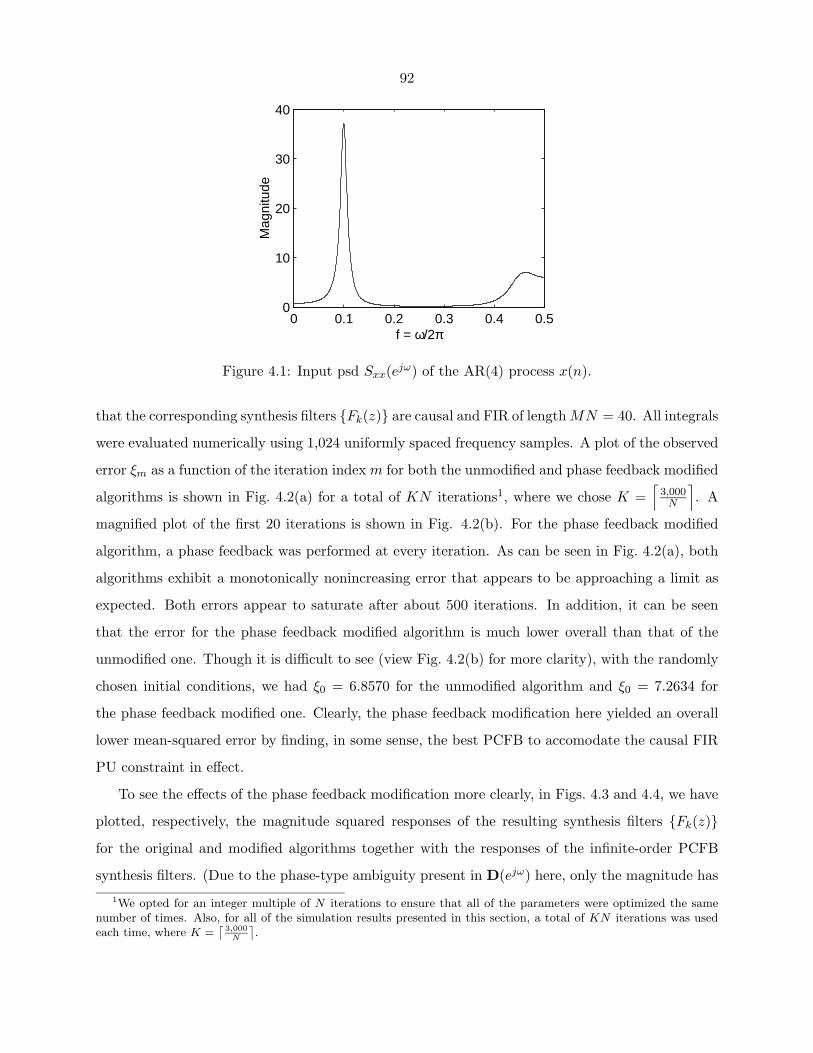
92

0 0.1 0.2 0.3 0.4 0.50

10

20

30

40

f = ω/2π

Mag

nitu

de

Figure 4.1: Input psd Sxx(ejω) of the AR(4) process x(n).

that the corresponding synthesis filters {Fk(z)} are causal and FIR of length MN = 40. All integrals

were evaluated numerically using 1,024 uniformly spaced frequency samples. A plot of the observed

error ξm as a function of the iteration index m for both the unmodified and phase feedback modified

algorithms is shown in Fig. 4.2(a) for a total of KN iterations1, where we chose K =⌈

3,000N

⌉. A

magnified plot of the first 20 iterations is shown in Fig. 4.2(b). For the phase feedback modified

algorithm, a phase feedback was performed at every iteration. As can be seen in Fig. 4.2(a), both

algorithms exhibit a monotonically nonincreasing error that appears to be approaching a limit as

expected. Both errors appear to saturate after about 500 iterations. In addition, it can be seen

that the error for the phase feedback modified algorithm is much lower overall than that of the

unmodified one. Though it is difficult to see (view Fig. 4.2(b) for more clarity), with the randomly

chosen initial conditions, we had ξ0 = 6.8570 for the unmodified algorithm and ξ0 = 7.2634 for

the phase feedback modified one. Clearly, the phase feedback modification here yielded an overall

lower mean-squared error by finding, in some sense, the best PCFB to accomodate the causal FIR

PU constraint in effect.

To see the effects of the phase feedback modification more clearly, in Figs. 4.3 and 4.4, we have

plotted, respectively, the magnitude squared responses of the resulting synthesis filters {Fk(z)}for the original and modified algorithms together with the responses of the infinite-order PCFB

synthesis filters. (Due to the phase-type ambiguity present in D(ejω) here, only the magnitude has1We opted for an integer multiple of N iterations to ensure that all of the parameters were optimized the same

number of times. Also, for all of the simulation results presented in this section, a total of KN iterations was usedeach time, where K =

⌈3,000

N

⌉.

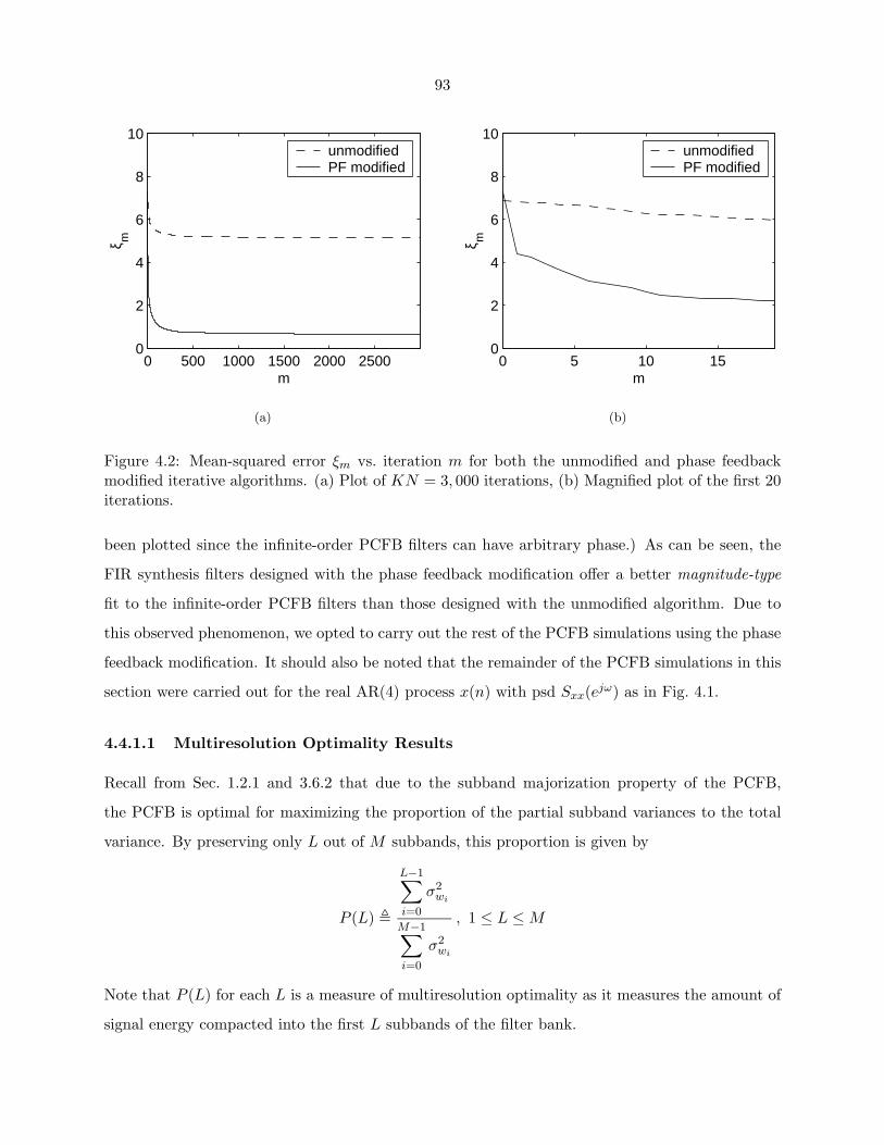
93

0 500 1000 1500 2000 25000

2

4

6

8

10

m

ξ m

unmodifiedPF modified

(a)

0 5 10 150

2

4

6

8

10

m

ξ m

unmodifiedPF modified

(b)

Figure 4.2: Mean-squared error ξm vs. iteration m for both the unmodified and phase feedbackmodified iterative algorithms. (a) Plot of KN = 3, 000 iterations, (b) Magnified plot of the first 20iterations.

been plotted since the infinite-order PCFB filters can have arbitrary phase.) As can be seen, the

FIR synthesis filters designed with the phase feedback modification offer a better magnitude-type

fit to the infinite-order PCFB filters than those designed with the unmodified algorithm. Due to

this observed phenomenon, we opted to carry out the rest of the PCFB simulations using the phase

feedback modification. It should also be noted that the remainder of the PCFB simulations in this

section were carried out for the real AR(4) process x(n) with psd Sxx(ejω) as in Fig. 4.1.

4.4.1.1 Multiresolution Optimality Results

Recall from Sec. 1.2.1 and 3.6.2 that due to the subband majorization property of the PCFB,

the PCFB is optimal for maximizing the proportion of the partial subband variances to the total

variance. By preserving only L out of M subbands, this proportion is given by

P (L) �

L−1∑i=0

σ2wi

M−1∑i=0

σ2wi

, 1 ≤ L ≤ M

Note that P (L) for each L is a measure of multiresolution optimality as it measures the amount of

signal energy compacted into the first L subbands of the filter bank.

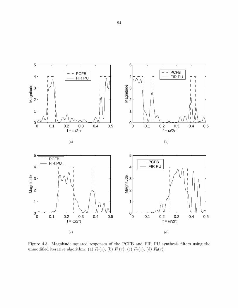
94

0 0.1 0.2 0.3 0.4 0.50

1

2

3

4

5

f = ω/2π

Mag

nitu

de

PCFBFIR PU

(a)

0 0.1 0.2 0.3 0.4 0.50

1

2

3

4

5

f = ω/2πM

agni

tude

PCFBFIR PU

(b)

0 0.1 0.2 0.3 0.4 0.50

1

2

3

4

5

f = ω/2π

Mag

nitu

de

PCFBFIR PU

(c)

0 0.1 0.2 0.3 0.4 0.50

1

2

3

4

5

f = ω/2π

Mag

nitu

de

PCFBFIR PU

(d)

Figure 4.3: Magnitude squared responses of the PCFB and FIR PU synthesis filters using theunmodified iterative algorithm. (a) F0(z), (b) F1(z), (c) F2(z), (d) F3(z).

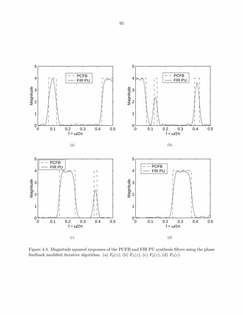
95

0 0.1 0.2 0.3 0.4 0.50

1

2

3

4

5

f = ω/2π

Mag

nitu

de

PCFBFIR PU

(a)

0 0.1 0.2 0.3 0.4 0.50

1

2

3

4

5

f = ω/2πM

agni

tude

PCFBFIR PU

(b)

0 0.1 0.2 0.3 0.4 0.50

1

2

3

4

5

f = ω/2π

Mag

nitu

de

PCFBFIR PU

(c)

0 0.1 0.2 0.3 0.4 0.50

1

2

3

4

5

f = ω/2π

Mag

nitu

de

PCFBFIR PU

(d)

Figure 4.4: Magnitude squared responses of the PCFB and FIR PU synthesis filters using the phasefeedback modified iterative algorithm. (a) F0(z), (b) F1(z), (c) F2(z), (d) F3(z).

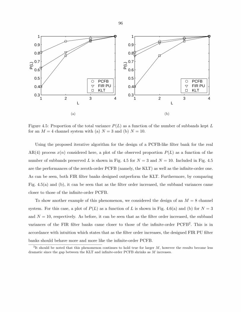
96

1 2 3 40.3

0.4

0.5

0.6

0.7

0.8

0.9

1

L

P(L

)

PCFBFIR PUKLT

(a)

1 2 3 40.3

0.4

0.5

0.6

0.7

0.8

0.9

1

L

P(L

)

PCFBFIR PUKLT

(b)

Figure 4.5: Proportion of the total variance P (L) as a function of the number of subbands kept Lfor an M = 4 channel system with (a) N = 3 and (b) N = 10.

Using the proposed iterative algorithm for the design of a PCFB-like filter bank for the real

AR(4) process x(n) considered here, a plot of the observed proportion P (L) as a function of the

number of subbands preserved L is shown in Fig. 4.5 for N = 3 and N = 10. Included in Fig. 4.5

are the performances of the zeroth-order PCFB (namely, the KLT) as well as the infinite-order one.

As can be seen, both FIR filter banks designed outperform the KLT. Furthermore, by comparing

Fig. 4.5(a) and (b), it can be seen that as the filter order increased, the subband variances came

closer to those of the infinite-order PCFB.

To show another example of this phenomenon, we considered the design of an M = 8 channel

system. For this case, a plot of P (L) as a function of L is shown in Fig. 4.6(a) and (b) for N = 3

and N = 10, respectively. As before, it can be seen that as the filter order increased, the subband

variances of the FIR filter banks came closer to those of the infinite-order PCFB2. This is in

accordance with intuition which states that as the filter order increases, the designed FIR PU filter

banks should behave more and more like the infinite-order PCFB.2It should be noted that this phenomenon continues to hold true for larger M , however the results become less

dramatic since the gap between the KLT and infinite-order PCFB shrinks as M increases.

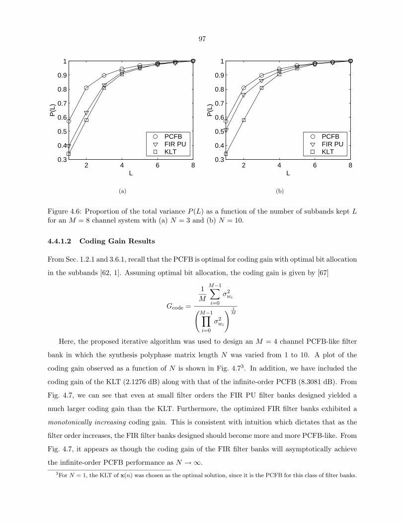
97

2 4 6 80.3

0.4

0.5

0.6

0.7

0.8

0.9

1

L

P(L

)

PCFBFIR PUKLT

(a)

2 4 6 80.3

0.4

0.5

0.6

0.7

0.8

0.9

1

L

P(L

)

PCFBFIR PUKLT

(b)

Figure 4.6: Proportion of the total variance P (L) as a function of the number of subbands kept Lfor an M = 8 channel system with (a) N = 3 and (b) N = 10.

4.4.1.2 Coding Gain Results

From Sec. 1.2.1 and 3.6.1, recall that the PCFB is optimal for coding gain with optimal bit allocation

in the subbands [62, 1]. Assuming optimal bit allocation, the coding gain is given by [67]

Gcode =

1M

M−1∑i=0

σ2wi(

M−1∏i=0

σ2wi

) 1M

Here, the proposed iterative algorithm was used to design an M = 4 channel PCFB-like filter

bank in which the synthesis polyphase matrix length N was varied from 1 to 10. A plot of the

coding gain observed as a function of N is shown in Fig. 4.73. In addition, we have included the

coding gain of the KLT (2.1276 dB) along with that of the infinite-order PCFB (8.3081 dB). From

Fig. 4.7, we can see that even at small filter orders the FIR PU filter banks designed yielded a

much larger coding gain than the KLT. Furthermore, the optimized FIR filter banks exhibited a

monotonically increasing coding gain. This is consistent with intuition which dictates that as the

filter order increases, the FIR filter banks designed should become more and more PCFB-like. From

Fig. 4.7, it appears as though the coding gain of the FIR filter banks will asymptotically achieve

the infinite-order PCFB performance as N → ∞.3For N = 1, the KLT of x(n) was chosen as the optimal solution, since it is the PCFB for this class of filter banks.

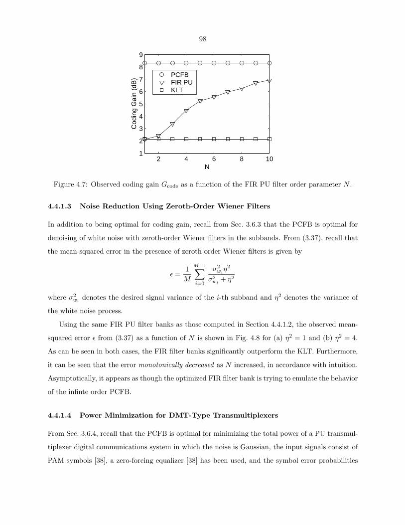
98

2 4 6 8 101

2

3

4

5

6

7

8

9

N

Cod

ing

Gai

n (d

B) PCFB

FIR PUKLT

Figure 4.7: Observed coding gain Gcode as a function of the FIR PU filter order parameter N .

4.4.1.3 Noise Reduction Using Zeroth-Order Wiener Filters

In addition to being optimal for coding gain, recall from Sec. 3.6.3 that the PCFB is optimal for

denoising of white noise with zeroth-order Wiener filters in the subbands. From (3.37), recall that

the mean-squared error in the presence of zeroth-order Wiener filters is given by

ε =1M

M−1∑i=0

σ2wi

η2

σ2wi

+ η2

where σ2wi

denotes the desired signal variance of the i-th subband and η2 denotes the variance of

the white noise process.

Using the same FIR PU filter banks as those computed in Section 4.4.1.2, the observed mean-

squared error ε from (3.37) as a function of N is shown in Fig. 4.8 for (a) η2 = 1 and (b) η2 = 4.

As can be seen in both cases, the FIR filter banks significantly outperform the KLT. Furthermore,

it can be seen that the error monotonically decreased as N increased, in accordance with intuition.

Asymptotically, it appears as though the optimized FIR filter bank is trying to emulate the behavior

of the infinte order PCFB.

4.4.1.4 Power Minimization for DMT-Type Transmultiplexers

From Sec. 3.6.4, recall that the PCFB is optimal for minimizing the total power of a PU transmul-

tiplexer digital communications system in which the noise is Gaussian, the input signals consist of

PAM symbols [38], a zero-forcing equalizer [38] has been used, and the symbol error probabilities

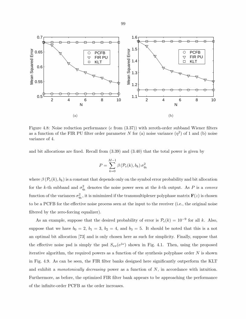
99

2 4 6 8 100.5

0.55

0.6

0.65

0.7

N

Mea

n S

quar

ed E

rror PCFB

FIR PUKLT

(a)

2 4 6 8 101.1

1.2

1.3

1.4

1.5

1.6

N

Mea

n S

quar

ed E

rror PCFB

FIR PUKLT

(b)

Figure 4.8: Noise reduction performance (ε from (3.37)) with zeroth-order subband Wiener filtersas a function of the FIR PU filter order parameter N for (a) noise variance (η2) of 1 and (b) noisevariance of 4.

and bit allocations are fixed. Recall from (3.39) and (3.40) that the total power is given by

P =M−1∑k=0

β (Pe(k), bk)σ2qk

where β (Pe(k), bk) is a constant that depends only on the symbol error probability and bit allocation

for the k-th subband and σ2qk

denotes the noise power seen at the k-th output. As P is a convex

function of the variances σ2qk

, it is minimized if the transmultiplexer polyphase matrix F(z) is chosen

to be a PCFB for the effective noise process seen at the input to the receiver (i.e., the original noise

filtered by the zero-forcing equalizer).

As an example, suppose that the desired probability of error is Pe(k) = 10−9 for all k. Also,

suppose that we have b0 = 2, b1 = 3, b2 = 4, and b3 = 5. It should be noted that this is a not

an optimal bit allocation [73] and is only chosen here as such for simplicity. Finally, suppose that

the effective noise psd is simply the psd Sxx(ejω) shown in Fig. 4.1. Then, using the proposed

iterative algorithm, the required powers as a function of the synthesis polyphase order N is shown

in Fig. 4.9. As can be seen, the FIR filter banks designed here significantly outperform the KLT

and exhibit a monotonically decreasing power as a function of N , in accordance with intuition.

Furthermore, as before, the optimized FIR filter bank appears to be approaching the performance

of the infinite-order PCFB as the order increases.

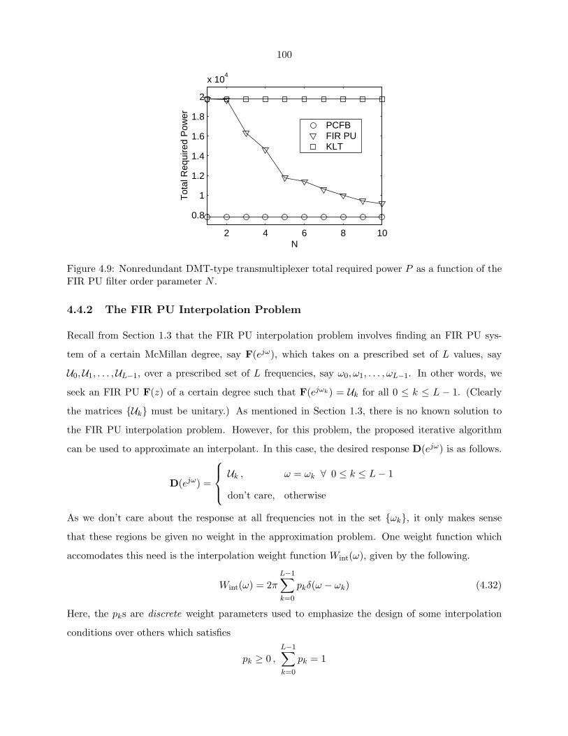
100

2 4 6 8 10

0.8

1

1.2

1.4

1.6

1.8

2

x 104

N

Tot

al R

equi

red

Pow

er

PCFBFIR PUKLT

Figure 4.9: Nonredundant DMT-type transmultiplexer total required power P as a function of theFIR PU filter order parameter N .

4.4.2 The FIR PU Interpolation Problem

Recall from Section 1.3 that the FIR PU interpolation problem involves finding an FIR PU sys-

tem of a certain McMillan degree, say F(ejω), which takes on a prescribed set of L values, say

U0,U1, . . . ,UL−1, over a prescribed set of L frequencies, say ω0, ω1, . . . , ωL−1. In other words, we

seek an FIR PU F(z) of a certain degree such that F(ejωk) = Uk for all 0 ≤ k ≤ L − 1. (Clearly

the matrices {Uk} must be unitary.) As mentioned in Section 1.3, there is no known solution to

the FIR PU interpolation problem. However, for this problem, the proposed iterative algorithm

can be used to approximate an interpolant. In this case, the desired response D(ejω) is as follows.

D(ejω) =

Uk , ω = ωk ∀ 0 ≤ k ≤ L − 1

don’t care, otherwise

As we don’t care about the response at all frequencies not in the set {ωk}, it only makes sense

that these regions be given no weight in the approximation problem. One weight function which

accomodates this need is the interpolation weight function Wint(ω), given by the following.

Wint(ω) = 2π

L−1∑k=0

pkδ(ω − ωk) (4.32)

Here, the pks are discrete weight parameters used to emphasize the design of some interpolation

conditions over others which satisfies

pk ≥ 0 ,L−1∑k=0

pk = 1

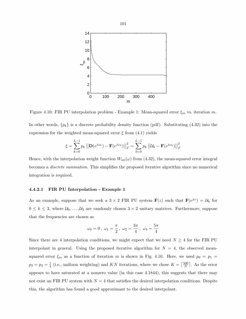
101

0 100 200 300 4000

2

4

6

8

10

12

14

m

ξ m

Figure 4.10: FIR PU interpolation problem - Example 1: Mean-squared error ξm vs. iteration m.

In other words, {pk} is a discrete probability density function (pdf). Substituting (4.32) into the

expression for the weighted mean-squared error ξ from (4.1) yields

ξ =L−1∑k=0

pk

∣∣∣∣D(ejωk) − F(ejωk)∣∣∣∣2

F=

L−1∑k=0

pk

∣∣∣∣Uk − F(ejωk)∣∣∣∣2

F

Hence, with the interpolation weight function Wint(ω) from (4.32), the mean-squared error integral

becomes a discrete summation. This simplifies the proposed iterative algorithm since no numerical

integration is required.

4.4.2.1 FIR PU Interpolation - Example 1

As an example, suppose that we seek a 3 × 2 FIR PU system F(z) such that F(ejω) = Uk for

0 ≤ k ≤ 3, where U0, . . . ,U3 are randomly chosen 3 × 2 unitary matrices. Furthermore, suppose

that the frequencies are chosen as

ω0 = 0 , ω1 =π

2, ω2 =

3π

4, ω3 =

5π

4

Since there are 4 interpolation conditions, we might expect that we need N ≥ 4 for the FIR PU

interpolant in general. Using the proposed iterative algorithm for N = 4, the observed mean-

squared error ξm as a function of iteration m is shown in Fig. 4.10. Here, we used p0 = p1 =

p2 = p3 = 14 (i.e., uniform weighting) and KN iterations, where we chose K =

⌈500N

⌉. As the error

appears to have saturated at a nonzero value (in this case 4.1844), this suggests that there may

not exist an FIR PU system with N = 4 that satisfies the desired interpolation conditions. Despite

this, the algorithm has found a good approximant to the desired interpolant.

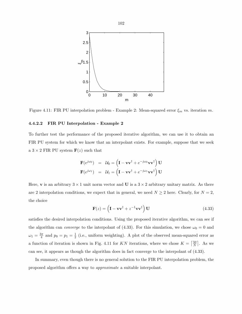
102

0 10 20 30 400

0.5

1

1.5

2

2.5

3

m

ξ m

Figure 4.11: FIR PU interpolation problem - Example 2: Mean-squared error ξm vs. iteration m.

4.4.2.2 FIR PU Interpolation - Example 2

To further test the performance of the proposed iterative algorithm, we can use it to obtain an

FIR PU system for which we know that an interpolant exists. For example, suppose that we seek

a 3 × 2 FIR PU system F(z) such that

F(ejω0) = U0 =(I − vv† + e−jω0vv†

)U

F(ejω1) = U1 =(I − vv† + e−jω1vv†

)U

Here, v is an arbitrary 3× 1 unit norm vector and U is a 3× 2 arbitrary unitary matrix. As there

are 2 interpolation conditions, we expect that in general, we need N ≥ 2 here. Clearly, for N = 2,

the choice

F(z) =(I − vv† + z−1vv†

)U (4.33)

satisfies the desired interpolation conditions. Using the proposed iterative algorithm, we can see if

the algorithm can converge to the interpolant of (4.33). For this simulation, we chose ω0 = 0 and

ω1 = 3π4 and p0 = p1 = 1

2 (i.e., uniform weighting). A plot of the observed mean-squared error as

a function of iteration is shown in Fig. 4.11 for KN iterations, where we chose K =⌈

50N

⌉. As we

can see, it appears as though the algorithm does in fact converge to the interpolant of (4.33).

In summary, even though there is no general solution to the FIR PU interpolation problem, the

proposed algorithm offers a way to approximate a suitable interpolant.

103

4.5 Concluding Remarks

Using the complete characterization of FIR PU systems in terms of Householder-like degree-one

building blocks, in this chapter we proposed an iterative greedy algorithm for solving a general

matrix version of the weighted least-squares approximation problem for an FIR PU approximant.

For cases in which the desired response matrix exhibited a phase-type ambiguity, which we formally

defined here, a phase feedback modification was proposed in which the phase of the FIR PU

approximant was fed back to the desired response. With this modification in effect, the resulting

algorithm was shown to still remain greedy and provide a better magnitude-type fit of the desired

response.

As opposed to most traditional signal-adapted filter bank design methods which optimize a

specific objective for which the PCFB is optimal, the method used here was to approximate the

infinite-order PCFB itself using a realizable FIR PU filter bank. In contrast to popular criteria for

signal-adapted design, such as the MOC of Chapter 3, which require a filter bank completion step

after a suitable FIR compaction filter has been computed, the method used here avoids this entirely

as all of the filters are found simultaneously. The advantage of this is that we avoid the problems

due to the nonuniqueness of the compaction filter, which plagued the method presented in Chapter

3 with an exponential increase in complexity. Through simulations presented here, it was shown

that the FIR PU filter banks designed monotonically behaved more and more like the infinite-order

PCFB as the filter order increased in terms of numerous objectives. This serves to bridge the gap

between the zeroth-order KLT and infinite-order PCFB. Together with the results of the design

method of Chapter 3, this phenomenon has not previously been reported in the literature.

In addition to being useful for the design of signal-adapted filter banks, we showed that the

iterative algorithm could also be used for the FIR PU interpolation problem. Though this problem

is still open, the algorithm always offers a way to approximate a desired interpolant, which may or

may not even exist. With simulations provided here, we showed that the algorithm could converge

to an interpolant, when one was known to exist. In essence, the algorithm provides us with a

numerical approach to solve a theoretically open problem.

104

Chapter 5

Coding Gain OptimalFIR Filter Banks

This chapter differs somewhat in theme from the rest of the chapters in that we focus on the design

of FIR signal-adapted filter banks in which no PU constraint is enforced. As opposed to traditional

filter bank design algorithms which enforce a PU or biorthogonality condition to be satisfied, we

make no such constraints here. The only constraint that we adhere to is that the analysis/synthesis

filters be FIR and hence realizable.

Here, the model we focus on is a uniform filter bank with scalar quantizers in the subbands.

Such a model is commonly used to achieve good lossy data compression in methods such as JPEG

and MP3 [41, 39]. The goal here is to choose the best analysis/synthesis filters, subject to an FIR

constraint, to minimize the filter bank mean-squared reconstruction error for a fixed bit allocation

among the quantizers. This is shown to be equivalent to maximizing the coding gain of the system.

Under the high bit rate assumption [25], we show how to derive the optimal analysis/synthesis

bank assuming that the corresponding synthesis/analysis bank is fixed. This will lead to an iterative

greedy algorithm for designing the filter bank where the analysis and synthesis banks are alternately

optimized.

Simulation results presented here show the versatility and merit of the proposed greedy algo-

rithm. By neglecting the effects of the quantizers, we show how the method can be used to design

an overdecimated filter bank which minimizes the mean-squared error of its output. Though the

PU constraint is not enforced here, we show that many similarities exist between these FIR filter

banks designed and optimal PU filter banks or PCFBs. In particular, we show that the FIR filters

designed appear to compact the energy of the input process, a property which is also shared with

the PCFB.

105

When we account for the effects of the quantizers, we show how the algorithm can be used to

design optimal FIR pre/postfilters for quantization. The performance in this case is measured in

terms of coding gain and distortion or mean-squared error. We compare the distortion observed

to the rate-distortion bound given by information theory [25, 10, 7]. It is shown that the method

comes close to this bound and comes closer when we increase the filter orders, as expected.

Finally, we consider the design of a maximally decimated system with quantizers in the sub-

bands. As before, the performance is measured in terms of coding gain and distortion. When

compared to the rate-distortion bound, it is shown that the method comes closer to the bound as

we increase the filter orders, in line with intuition. Furthermore, we show that the quantized filter

bank system outperforms the scalar pre/postfiltering quantization system, as expected.

The content of portions of this chapter will be presented at [58].

5.1 Outline

In Sec. 5.2, we present the quantized filter bank model which we will focus on here. There, we

review the high bit rate assumption for scalar quantizers, which greatly simplifies the mathematical

analysis required for the objective under consideration.

In Sec. 5.3, we derive the optimal analysis/synthesis banks for minimizing the reconstruction

error at the output. The optimal synthesis bank for a fixed analysis bank is derived in Sec. 5.3.1,

whereas the optimal analysis bank for a fixed synthesis bank is derived in Sec. 5.3.2. In Sec. 5.3.3,

we formally present an iterative greedy algorithm for obtaining the optimal FIR filter bank for

minimizing the reconstruction error.

Simulation results are presented in Sec. 5.4. In Sec. 5.4.1, we neglect the effects due to quanti-

zation and show how the algorithm can be used to design an overdecimated filter bank. There, in

Sec. 5.4.1.1 and Sec. 5.4.1.2, the similarities and differences between the FIR filter banks designed

and the PCFB are shown. The effects of quantization are discussed in Sec. 5.4.2 along with several

important measures of optimality. In Sec. 5.4.2.1, we use the iterative algorithm to design optimal

FIR pre/postfilters for quantization. The method is shown there to exhibit distortion behavior close

to the rate-distortion bound. In Sec. 5.4.2.2, we consider the design of a maximally decimated filter

bank with quantizers in the subbands. There, it is shown that such filter banks yield performance

close to the rate-distortion bound and outperform the scalar pre/postfiltering quantization system.

Finally, concluding remarks are made in Sec. 5.5.

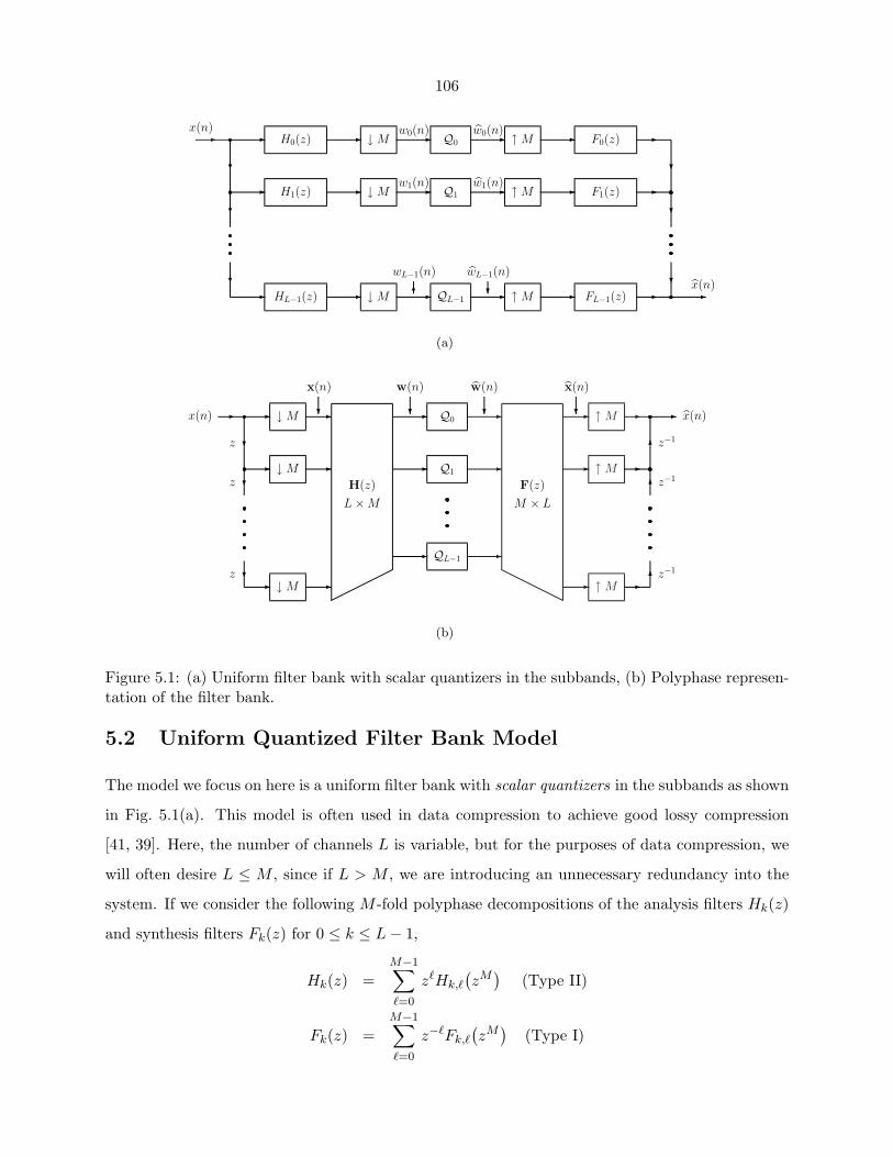
106

� � H0(z)

�

� H1(z)

�

�

� HL−1(z)

�

�

�

↓ M

↓ M

↓ M

�

�

�

x(n) w0(n)

w1(n)

wL−1(n)

�

Q0

Q1

QL−1

�

�

�

↑ M

↑ M

↑ M

�

�

�

F0(z)

F1(z)

FL−1(z)

�

�

�

�

�

�

�x(n)

w0(n)

w1(n)

wL−1(n)

�

(a)

�

�

�

�

�

�

↑ M

↑ M

↑ M

�

�

�

�

z−1

z−1

z−1

x(n)

x(n)

�

F(z)

M × L

w(n)

��

�

�

↓ M

↓ M

↓ M

�

�

�

�

�

�

� �

�

�

Q0

Q1

QL−1

w(n)

�x(n)

z

z

z

x(n)

�

H(z)

L × M

(b)

Figure 5.1: (a) Uniform filter bank with scalar quantizers in the subbands, (b) Polyphase represen-tation of the filter bank.

5.2 Uniform Quantized Filter Bank Model

The model we focus on here is a uniform filter bank with scalar quantizers in the subbands as shown

in Fig. 5.1(a). This model is often used in data compression to achieve good lossy compression

[41, 39]. Here, the number of channels L is variable, but for the purposes of data compression, we

will often desire L ≤ M , since if L > M , we are introducing an unnecessary redundancy into the

system. If we consider the following M -fold polyphase decompositions of the analysis filters Hk(z)

and synthesis filters Fk(z) for 0 ≤ k ≤ L − 1,

Hk(z) =M−1∑�=0

z�Hk,�

(zM

)(Type II)

Fk(z) =M−1∑�=0

z−�Fk,�

(zM

)(Type I)

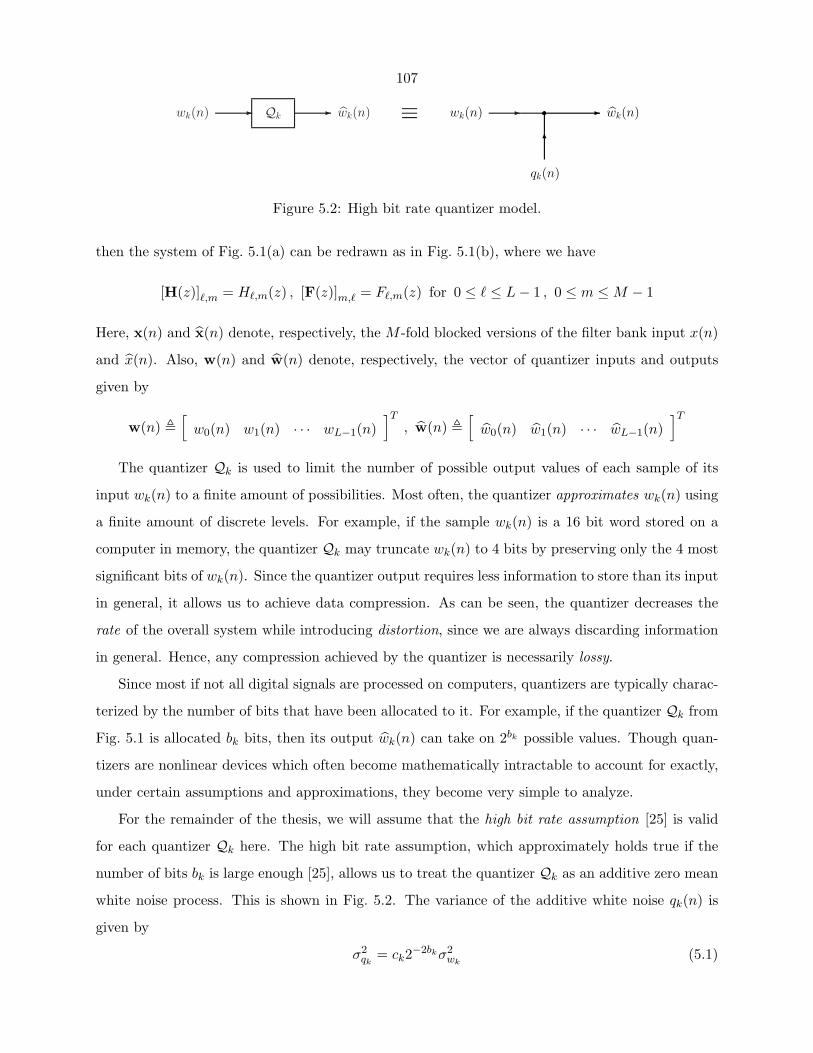
107

� Qk�wk(n) wk(n) � �

wk(n) wk(n)

qk(n)

≡

Figure 5.2: High bit rate quantizer model.

then the system of Fig. 5.1(a) can be redrawn as in Fig. 5.1(b), where we have

[H(z)]�,m = H�,m(z) , [F(z)]m,� = F�,m(z) for 0 ≤ � ≤ L − 1 , 0 ≤ m ≤ M − 1

Here, x(n) and x(n) denote, respectively, the M -fold blocked versions of the filter bank input x(n)

and x(n). Also, w(n) and w(n) denote, respectively, the vector of quantizer inputs and outputs

given by

w(n) �[

w0(n) w1(n) · · · wL−1(n)]T

, w(n) �[

w0(n) w1(n) · · · wL−1(n)]T

The quantizer Qk is used to limit the number of possible output values of each sample of its

input wk(n) to a finite amount of possibilities. Most often, the quantizer approximates wk(n) using

a finite amount of discrete levels. For example, if the sample wk(n) is a 16 bit word stored on a

computer in memory, the quantizer Qk may truncate wk(n) to 4 bits by preserving only the 4 most

significant bits of wk(n). Since the quantizer output requires less information to store than its input

in general, it allows us to achieve data compression. As can be seen, the quantizer decreases the

rate of the overall system while introducing distortion, since we are always discarding information

in general. Hence, any compression achieved by the quantizer is necessarily lossy.

Since most if not all digital signals are processed on computers, quantizers are typically charac-

terized by the number of bits that have been allocated to it. For example, if the quantizer Qk from

Fig. 5.1 is allocated bk bits, then its output wk(n) can take on 2bk possible values. Though quan-

tizers are nonlinear devices which often become mathematically intractable to account for exactly,

under certain assumptions and approximations, they become very simple to analyze.

For the remainder of the thesis, we will assume that the high bit rate assumption [25] is valid

for each quantizer Qk here. The high bit rate assumption, which approximately holds true if the

number of bits bk is large enough [25], allows us to treat the quantizer Qk as an additive zero mean

white noise process. This is shown in Fig. 5.2. The variance of the additive white noise qk(n) is

given by

σ2qk

= ck2−2bkσ2wk

(5.1)

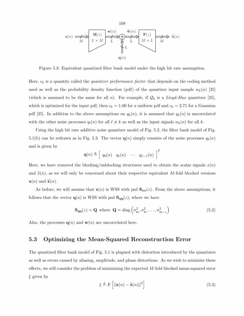
108

H(z)

L × MM L

w(n)

L

q(n)

L

w(n)F(z)

M × L Mx(n)x(n)

Figure 5.3: Equivalent quantized filter bank model under the high bit rate assumption.

Here, ck is a quantity called the quantizer performance factor that depends on the coding method

used as well as the probability density function (pdf) of the quantizer input sample wk(n) [25]

(which is assumed to be the same for all n). For example, if Qk is a Lloyd-Max quantizer [25],

which is optimized for the input pdf, then ck = 1.00 for a uniform pdf and ck = 2.71 for a Gaussian

pdf [25]. In addition to the above assumptions on qk(n), it is assumed that qk(n) is uncorrelated

with the other noise processes q�(n) for all � �= k as well as the input signals wk(n) for all k.

Using the high bit rate additive noise quantizer model of Fig. 5.2, the filter bank model of Fig.

5.1(b) can be redrawn as in Fig. 5.3. The vector q(n) simply consists of the noise processes qk(n)

and is given by

q(n) �[

q0(n) q1(n) · · · qL−1(n)]T

Here, we have removed the blocking/unblocking structures used to obtain the scalar signals x(n)

and x(n), as we will only be concerned about their respective equivalent M -fold blocked versions

x(n) and x(n).

As before, we will assume that x(n) is WSS with psd Sxx(z). From the above assumptions, it

follows that the vector q(n) is WSS with psd Sqq(z), where we have

Sqq(z) = Q where Q = diag(σ2

q0, σ2

q1, . . . , σ2

qL−1

)(5.2)

Also, the processes q(n) and w(n) are uncorrelated here.

5.3 Optimizing the Mean-Squared Reconstruction Error

The quantized filter bank model of Fig. 5.1 is plagued with distortion introduced by the quantizers

as well as errors caused by aliasing, amplitude, and phase distortions. As we wish to minimize these

effects, we will consider the problem of minimizing the expected M -fold blocked mean-squared error

ξ given by

ξ � E[||x(n) − x(n)||2

](5.3)

109

for a fixed bit allocation {bk}. Using the high bit rate model of the quantized filter bank shown

in Fig. 5.3, it follows that x(n) and x(n) are jointly WSS. Hence, the error e(n) � x(n) − x(n) is

WSS. We have

ξ = E[e†(n)e(n)

]= Tr

[E[e(n)e†(n)

]]= Tr [Ree(0)] = Tr

[12π

∫ 2π

0See(ejω) dω

](5.4)

where Ree(k) and See(z) denote, respectively, the autocorrelation and psd of e(n). As e(n) =

x(n) − x(n), we have

See(z) = Sxx(z) − Sxx(z) − Sxx(z) + Sxx(z) (5.5)

where Sxx(z) and Sxx(z) denote the cross psds of x(n) and x(n) [48], and Sxx(z) denotes the psd

of x(n). Note that from Fig. 5.3, we have

X(z) = F(z)H(z)X(z) + F(z)Q(z)

Thus, assuming x(n) and q(n) are uncorrelated, we have [67]

Sxx(z) = Sxx(z)H(z)F(z) (5.6)

Sxx(z) = Sxx(z) = F(z)H(z)Sxx(z) (5.7)

Sxx(z) = F(z)H(z)Sxx(z)H(z)F(z) + F(z)Sqq(z)F(z)

= F(z)H(z)Sxx(z)H(z)F(z) + F(z)QF(z) (5.8)

Here, we used (5.2) in (5.8). Substituting (5.6), (5.7), and (5.8) in (5.5), we get

See(z) = Sxx(z) − Sxx(z)H(z)F(z) − F(z)H(z)Sxx(z)

+ F(z)H(z)Sxx(z)H(z)F(z) + F(z)QF(z)(5.9)

Though it is difficult to jointly choose H(z) and F(z) subject to FIR constraints to optimize ξ

(see [20, 19, 21] for a Lagrange multiplier technique for a fixed quantization term Q), doing so one

at a time is simple and can be done globally. This will lead to an iterative algorithm whereby the

analysis and synthesis banks are alternately optimized. Before proceeding, note that the matrix Q

from (5.9) depends on the analysis bank H(z). To see this, note that from (5.2) and (5.1), we have

Q = diag(c02−2b0σ2

w0, c12−2b1σ2

w1, . . . , cL−12−2bL−1σ2

wL−1

)(5.10)

where we have, from Fig. 5.3,

σ2wk

=12π

∫ 2π

0

[H(ejω)Sxx(ejω)H†(ejω)

]k,k

dω (5.11)

Hence, optimizing the analysis bank H(z) for a fixed synthesis bank F(z) is more mathematically

challenging than optimizing F(z) for a fixed H(z). As such, we first consider optimizing F(z) for

a fixed H(z) and then move on to the more challenging task of optimizing H(z) for a fixed F(z).

110

5.3.1 Optimal Synthesis Bank F(z) for Fixed Analysis Bank H(z)

Suppose that the analysis bank H(z) is fixed and that the synthesis bank F(z) is FIR of length Nf

and of the form

F(z) = zPFc(z)

where P is an advance parameter and Fc(z) is a causal FIR system of the form

Fc(z) =Nf−1∑n=0

fc(n)z−n

Note that the impulse response fc(n) is an M × L sequence. If we define the M × LNf matrix f c

and LNf × L delay matrix d(z) as

f c �[

fc(0) fc(1) · · · fc(Nf − 1)]

d(z) �[

zP IL zP−1IL · · · zP−(Nf−1)IL

]T

then clearly we have F(z) = f cd(z) and all of the degrees of freedom in choosing F(z) with the FIR

constraint lie in the choice of the constant matrix f c. From (5.9), we have

See(z) = Sxx(z) − Sxx(z)H(z)d(z)f †c − f cd(z)H(z)Sxx(z)

+ f cd(z)[H(z)Sxx(z)H(z) + Q

]d(z)f †c

(5.12)

Substituting (5.12) into (5.4) yields

ξ = Tr[Rxx(0) − B†f †c − f cB + f cAf

†c

](5.13)

where Rxx(k) denotes the autocorrelation of x(n) and the LNf × LNf matrix A and LNf × M

matrix B are defined as follows.

A � 12π

∫ 2π

0d(ejω)

[H(ejω)Sxx(ejω)H†(ejω) + Q

]d†(ejω) dω (5.14)

B � 12π

∫ 2π

0d(ejω)H(ejω)Sxx(ejω) dω (5.15)

Note that A is simply the Nf -fold block autocorrelation matrix of the process w(n) from Fig. 5.3

[48]. In other words, if Rww(k) denotes the autocorrelation of w(n), then we have

A =

Rww(0) Rww(1) · · · Rww(Nf − 1)

Rww(−1) Rww(0) · · · Rww(Nf − 2)...

.... . .

...

Rww(−(Nf − 1)) Rww(−(Nf − 2)) · · · Rww(0)

111

As such, the matrix A is strictly positive definite and hence invertible [48]. Since A is invertible,

using the trick of completing the square [22, 34], we can express ξ in (5.13) as follows

ξ = Tr[ (

f c − B†A−1)A(f c − B†A−1

)†︸ ︷︷ ︸

positive semidefinite

+Rxx(0) − B†A−1B]

As we wish to minimize ξ, this can only be done by setting the first term on the right-hand side

of the above equation equal to the zero matrix. This yields the following optimal choice of f c and

corresponding optimal ξ.

f c,opt = B†A−1 , ξopt = Tr[Rxx(0) − B†A−1B

](5.16)

Here, A and B are as in (5.14) and (5.15), respectively. The choice of f c given in (5.16) is optimal

for a fixed Sxx(z), H(z), and Q.

5.3.2 Optimal Analysis Bank H(z) for Fixed Synthesis Bank F(z)

5.3.2.1 Simplifying the Quantization Noise Term

Prior to optimizing the mean-squared error ξ with respect to the analysis bank H(z), it will help to

simplify the quantization noise term that appears in the expression for See(z) given in (5.9). Note

that from (5.4), we have

ξ =12π

∫ 2π

0Tr[See(ejω)

]dω (5.17)

Also, from (5.9), we have

Tr [See(z)] = Tr [Sxx(z)] − Tr[Sxx(z)H(z)F(z)

]− Tr [F(z)H(z)Sxx(z)]

+ Tr[F(z)H(z)Sxx(z)H(z)F(z)

]+ Tr

[F(z)QF(z)

]︸ ︷︷ ︸

G(z)

(5.18)

Before simplifying Tr [See(z)] further, we will simplify the term G(z), which is due to the

quantization noise q(n) filtered by the synthesis bank F(z) as can be seen in Fig. 5.3. The reason

for this is that the matrix Q appearing in G(z) depends on the analysis bank H(z) as can be seen

from (5.10) and (5.11). Using the fact that Tr [AB] = Tr [BA] whenever A and B are conformable

[22], we have

G(z) = Tr[QF(z)F(z)

]Upon using (5.10), we get

G(z) =L−1∑k=0

ck2−2bkσ2yk

[F(z)F(z)

]k,k

=L−1∑k=0

ck2−2bk

[F(z)F(z)

]k,k

σ2yk

112

As σ2yk

is given by (5.11), we have

G(z) =L−1∑k=0

ck2−2bk

[F(z)F(z)

]k,k

(12π

∫ 2π

0

[H(ejλ)Sxx(ejλ)H†(ejλ)

]k,k

dλ

)

=12π

∫ 2π

0

(L−1∑k=0

ck2−2bk

[F(z)F(z)

]k,k

[H(ejλ)Sxx(ejλ)H†(ejλ)

]k,k

)dλ (5.19)

Define the L × L matrix Λ(z) as follows.

Λ(z) � diag(

c02−2b0[F(z)F(z)

]0,0

, c12−2b1[F(z)F(z)

]1,1

, . . . , cL−12−2bL−1

[F(z)F(z)

]L−1,L−1

)(5.20)

Note that Λ(z) does not depend on H(z). Using Λ(z) in (5.19), we can express G(z) as

G(z) =12π

∫ 2π

0Tr[Λ(z)H(ejλ)Sxx(ejλ)H†(ejλ)

]dλ (5.21)

With the simplification of the noise term G(z) given in (5.21), we are now ready to optimize ξ

with respect to H(z) with an FIR constraint in effect.

5.3.2.2 Imposing the FIR Constraint on H(z)

Suppose now that the synthesis bank F(z) is fixed and that the analysis bank H(z) is FIR of length

Nh and of the form

H(z) = zQHc(z)

where Q is an advance parameter and Hc(z) is a causal FIR system of the form

Hc(z) =Nh−1∑n=0

hc(n)z−n

Note that the impulse response hc(n) is an L × M sequence and that there are Nh such matrix

coefficients. Hence, H(z) is characterized by a total of LMNh degrees of freedom with the FIR

constraint in effect. In order to minimize ξ from (5.17) in this case, we need to group all of these

degrees of freedom together, which can be done through the use of the vec operator [34].

Recall that if A is any M × N matrix, then vec(A) is an MN × 1 column vector with [34]

[vec(A)]k � [A]k mod M,� kM � , 0 ≤ k ≤ MN − 1

In other words, the vec operator stacks the columns of any matrix on top of each other creating

a large column vector. Through clever use of the vec operator, we can express ξ from (5.17) as a

quadratic function in terms of the filter coefficients of H(z).

113

For simplicity, define the LM × 1 column vectors hn as follows.

hn � vec (hc(n)) , 0 ≤ n ≤ Nh − 1

Furthermore, define the LMNh×1 vector h, the LM ×1 vector v(z) and the LMNh×LM advance

matrix a(z) as follows.

h �[

hT0 h

T1 · · · h

TNh−1

]T

v(z) � vec(F(z)Sxx(z)

)a(z) �

[z−QILM z1−QILM · · · zNh−1−QILM

]T

Note that h contains all of the degrees of freedom of H(z) here. Also note that due to the linearity

property of the vec operator [34], we have

vec (H(z)) =Nh−1∑n=0

zQ−n vec (hc(n))︸ ︷︷ ︸hn

=[

zQILM zQ−1ILM · · · zQ−(Nh−1)ILM

]︸ ︷︷ ︸

a(z)

h0

h1

...

hNh−1

︸ ︷︷ ︸

h

(5.22)

By exploiting the following properties of the trace and vec operators [34],

Tr[A†B

]= (vec(A))† vec(B) (5.23)

vec(AXB) =(BT ⊗ A

)vec(X) (5.24)

where ⊗ denotes the Kronecker product operator [34], we can express the error ξ as a quadratic

function of the vector h, which can then be minimized by completing the square as was done in

Sec. 5.3.1. Note that for any M ×N matrix A and P ×Q matrix B, the Kronecker product A⊗B

is a MP × NQ matrix defined as follows [34].

A ⊗ B �

[A]0,0 B [A]0,1 B · · · [A]0,N−1 B

[A]1,0 B [A]1,1 B · · · [A]1,N−1 B...

.... . .

...

[A]M−1,0 B [A]M−1,1 B · · · [A]M−1,N−1 B

114

Substituting (5.21) into (5.18) and exploiting (5.23), (5.24), and (5.22), we have the following.

Tr [See(z)] = Tr [Sxx(z)] − Tr[H(z)F(z)Sxx(z)

]− Tr [Sxx(z)F(z)H(z)]

+ Tr[H(z)F(z)F(z)H(z)Sxx(z)

]+

12π

∫ 2π

0Tr[H†(ejλ)Λ(z)H(ejλ)Sxx(ejλ)

]dλ

= Tr [Sxx(z)] − h†a(z)v(z) − v(z)a(z)h

+ h†a(z) vec

(F(z)F(z)H(z)Sxx(z)

)+

12π

∫ 2π

0h†a(ejλ) vec

(Λ(z)H(ejλ)Sxx(ejλ)

)dλ

= Tr [Sxx(z)] − h†a(z)v(z) − v(z)a(z)h

+ h†a(z)

(ST

xx(z) ⊗ F(z)F(z))a(z)h

+ h†(

12π

∫ 2π

0a(ejλ)

(ST

xx(ejλ) ⊗ Λ(z))a†(ejλ) dλ

)h (5.25)

Upon substituting (5.25) into (5.17), we get the following.

ξ = Tr [Rxx(0)] − h†g − g†h + h

†Ch (5.26)

where the LMNh × 1 vector g and LMNh × LMNh matrix C are defined as

g � 12π

∫ 2π

0a(ejω)v(ejω) dω (5.27)

C � 12π

∫ 2π

0a(ejω)

(ST

xx(ejω) ⊗(F†(ejω)F(ejω) + D

))a†(ejω) dω (5.28)

and the L × L matrix D is defined to be

D � 12π

∫ 2π

0Λ(ejω) dω

where Λ(z) is as in (5.20).

As can be seen from (5.26), the mean-squared error ξ is a quadratic function of the coefficients

of H(z) which are contained in the vector h. To minimize ξ from (5.26), we can complete the

square as was done in Sec. 5.3.1. In order to do so, first note that the matrix C from (5.28) is

invertible. To see this, note that from (5.8), h†Ch represents the energy of x(n) from Fig. 5.3, i.e.,

h†Ch = Tr [Rxx(0)] > 0 for all h �= 0, since we assume that the energy of x(n) is nonzero here.

Hence, by completing the square [22], the optimal h and corresponding optimal ξ are given by

hopt = C−1g , ξopt = Tr [Rxx(0)] − g†C−1g (5.29)

Here, g and C are given by (5.27) and (5.28), respectively. The choice of h given in (5.29) is optimal

for a fixed Sxx(z), F(z), {ck}, and {bk}.

115

5.3.3 Iterative Greedy Analysis/Synthesis Filter Bank Optimization Algorithm

By alternately optimizing the analysis and synthesis banks, we obtain an iterative greedy algorithm

for designing an FIR filter bank adapted to the psd Sxx(z) and the bit allocation {bk}. In what

follows, let Fk(z), Hk(z), and ξk denote, respectively, the synthesis bank, analysis bank, and

reconstruction error at the k-th iteration for k ≥ 0. Then, the iterative filter bank optimization

algorithm is as follows.

Initialization:

1. Select a set of values for the desired filter bank parameters L, M , P , Nf , Q, and Nh.

2. Select a desired bit allocation {bk} along the subbands and choose appropriate quantizer

performance factors {ck} for the subband pdfs.

3. Choose an initial synthesis bank F0(z).

4. Compute the corresponding optimal analysis bank H0(z) and reconstruction error ξ0

using (5.29).

Iteration: For k ≥ 1, do the following.

1. With a fixed analysis bank Hk−1(z), compute the optimal synthesis bank Fk(z) using

(5.16).

2. With a fixed synthesis bank Fk(z), compute the optimal analysis bank Hk(z) and cor-

responding reconstruction error ξk using (5.29).

3. Increment k by 1 and return to Step 1.

Since this algorithm is greedy, the error ξk is guaranteed to be a monotonic nonincreasing

function of the iteration index k. As the error is always lower bounded by zero (i.e., ξk ≥ 0), ξk

is also guaranteed to have a limit as k → ∞ [67]. Simulation results provided here verify this

monotonic and limiting behavior. In particular, it will be seen that the error appears to quickly

converge to its limit after only a few iterations.

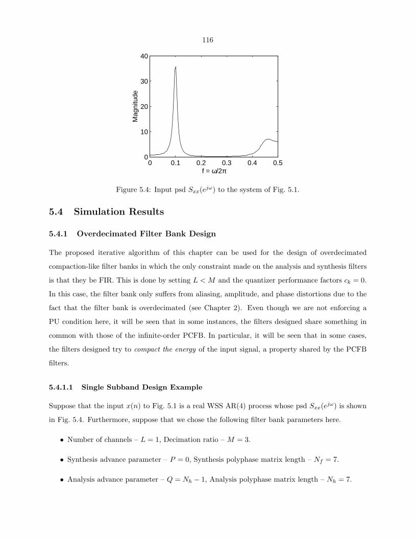
116

0 0.1 0.2 0.3 0.4 0.50

10

20

30

40

f = ω/2π

Mag

nitu

de

Figure 5.4: Input psd Sxx(ejω) to the system of Fig. 5.1.

5.4 Simulation Results

5.4.1 Overdecimated Filter Bank Design

The proposed iterative algorithm of this chapter can be used for the design of overdecimated

compaction-like filter banks in which the only constraint made on the analysis and synthesis filters

is that they be FIR. This is done by setting L < M and the quantizer performance factors ck = 0.

In this case, the filter bank only suffers from aliasing, amplitude, and phase distortions due to the

fact that the filter bank is overdecimated (see Chapter 2). Even though we are not enforcing a

PU condition here, it will be seen that in some instances, the filters designed share something in

common with those of the infinite-order PCFB. In particular, it will be seen that in some cases,

the filters designed try to compact the energy of the input signal, a property shared by the PCFB

filters.

5.4.1.1 Single Subband Design Example

Suppose that the input x(n) to Fig. 5.1 is a real WSS AR(4) process whose psd Sxx(ejω) is shown

in Fig. 5.4. Furthermore, suppose that we chose the following filter bank parameters here.

• Number of channels – L = 1, Decimation ratio – M = 3.

• Synthesis advance parameter – P = 0, Synthesis polyphase matrix length – Nf = 7.

• Analysis advance parameter – Q = Nh − 1, Analysis polyphase matrix length – Nh = 7.

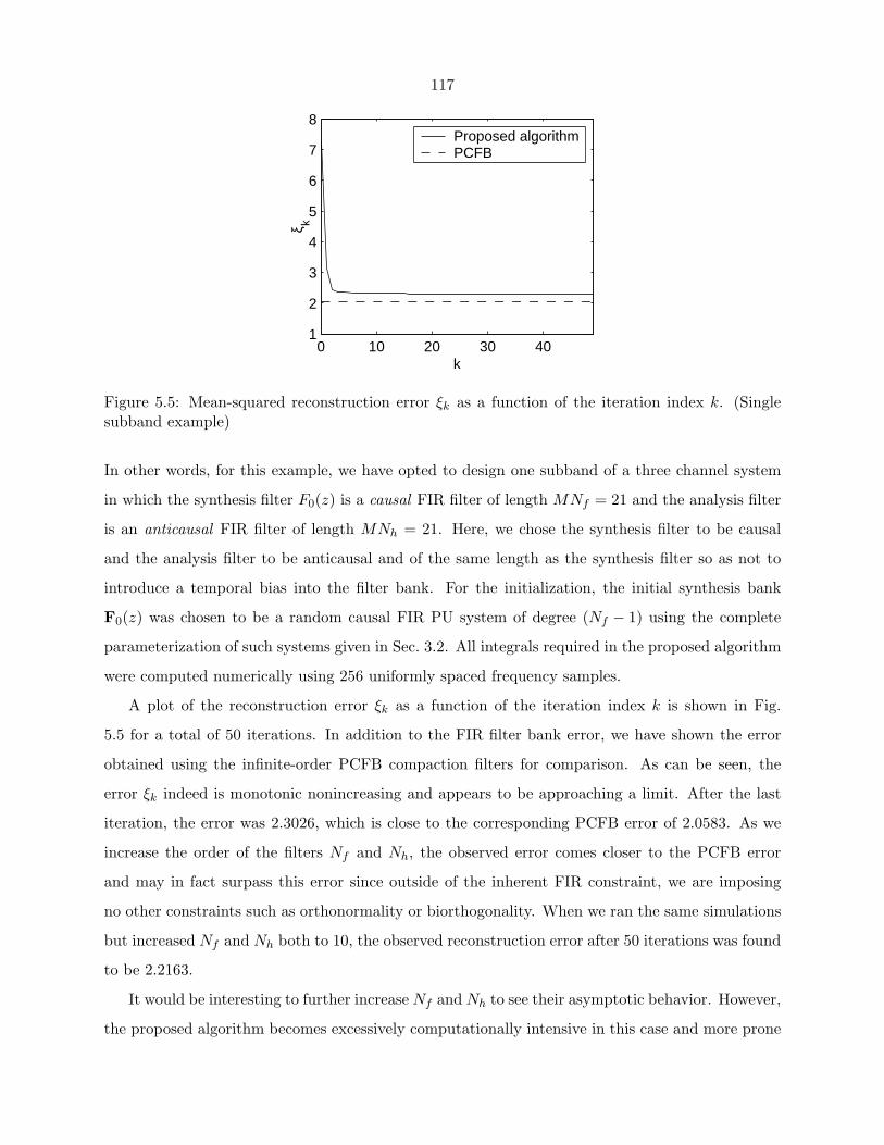
117

0 10 20 30 401

2

3

4

5

6

7

8

k

ξ k

Proposed algorithmPCFB

Figure 5.5: Mean-squared reconstruction error ξk as a function of the iteration index k. (Singlesubband example)

In other words, for this example, we have opted to design one subband of a three channel system

in which the synthesis filter F0(z) is a causal FIR filter of length MNf = 21 and the analysis filter

is an anticausal FIR filter of length MNh = 21. Here, we chose the synthesis filter to be causal

and the analysis filter to be anticausal and of the same length as the synthesis filter so as not to

introduce a temporal bias into the filter bank. For the initialization, the initial synthesis bank

F0(z) was chosen to be a random causal FIR PU system of degree (Nf − 1) using the complete

parameterization of such systems given in Sec. 3.2. All integrals required in the proposed algorithm

were computed numerically using 256 uniformly spaced frequency samples.

A plot of the reconstruction error ξk as a function of the iteration index k is shown in Fig.

5.5 for a total of 50 iterations. In addition to the FIR filter bank error, we have shown the error

obtained using the infinite-order PCFB compaction filters for comparison. As can be seen, the

error ξk indeed is monotonic nonincreasing and appears to be approaching a limit. After the last

iteration, the error was 2.3026, which is close to the corresponding PCFB error of 2.0583. As we

increase the order of the filters Nf and Nh, the observed error comes closer to the PCFB error

and may in fact surpass this error since outside of the inherent FIR constraint, we are imposing

no other constraints such as orthonormality or biorthogonality. When we ran the same simulations

but increased Nf and Nh both to 10, the observed reconstruction error after 50 iterations was found

to be 2.2163.

It would be interesting to further increase Nf and Nh to see their asymptotic behavior. However,

the proposed algorithm becomes excessively computationally intensive in this case and more prone

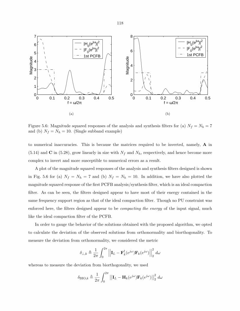
118

0 0.1 0.2 0.3 0.4 0.50

1

2

3

4

5

6

7

f = ω/2π

Mag

nitu

de

|H0(ejω)|2

|F0(ejω)|2

1st PCFB

(a)

0 0.1 0.2 0.3 0.4 0.50

2

4

6

8

f = ω/2π

Mag

nitu

de

|H0(ejω)|2

|F0(ejω)|2

1st PCFB

(b)

Figure 5.6: Magnitude squared responses of the analysis and synthesis filters for (a) Nf = Nh = 7and (b) Nf = Nh = 10. (Single subband example)

to numerical inaccuracies. This is because the matrices required to be inverted, namely, A in

(5.14) and C in (5.28), grow linearly in size with Nf and Nh, respectively, and hence become more

complex to invert and more susceptible to numerical errors as a result.

A plot of the magnitude squared responses of the analysis and synthesis filters designed is shown

in Fig. 5.6 for (a) Nf = Nh = 7 and (b) Nf = Nh = 10. In addition, we have also plotted the

magnitude squared response of the first PCFB analysis/synthesis filter, which is an ideal compaction

filter. As can be seen, the filters designed appear to have most of their energy contained in the

same frequency support region as that of the ideal compaction filter. Though no PU constraint was

enforced here, the filters designed appear to be compacting the energy of the input signal, much

like the ideal compaction filter of the PCFB.

In order to gauge the behavior of the solutions obtained with the proposed algorithm, we opted

to calculate the deviation of the observed solutions from orthonormality and biorthogonality. To

measure the deviation from orthonormality, we considered the metric

δ⊥,k � 12π

∫ 2π

0

∣∣∣∣∣∣IL − F†k(e

jω)Fk(ejω)∣∣∣∣∣∣2

2dω

whereas to measure the deviation from biorthogonality, we used

δBIO,k � 12π

∫ 2π

0

∣∣∣∣IL − Hk(ejω)Fk(ejω)∣∣∣∣2

2dω

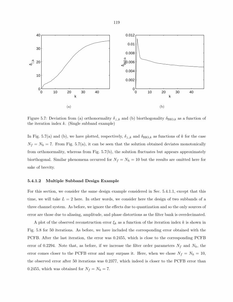
119

0 10 20 30 400

10

20

30

40

k

δ ⊥,k

(a)

0 10 20 30 400

0.002

0.004

0.006

0.008

0.01

0.012

k

δ BIO

,k

(b)

Figure 5.7: Deviation from (a) orthonormality δ⊥,k and (b) biorthogonality δBIO,k as a function ofthe iteration index k. (Single subband example)

In Fig. 5.7(a) and (b), we have plotted, respectively, δ⊥,k and δBIO,k as functions of k for the case

Nf = Nh = 7. From Fig. 5.7(a), it can be seen that the solution obtained deviates monotonically

from orthonormality, whereas from Fig. 5.7(b), the solution fluctuates but appears approximately

biorthogonal. Similar phenomena occurred for Nf = Nh = 10 but the results are omitted here for

sake of brevity.

5.4.1.2 Multiple Subband Design Example

For this section, we consider the same design example considered in Sec. 5.4.1.1, except that this

time, we will take L = 2 here. In other words, we consider here the design of two subbands of a

three channel system. As before, we ignore the effects due to quantization and so the only sources of

error are those due to aliasing, amplitude, and phase distortions as the filter bank is overdecimated.

A plot of the observed reconstruction error ξk as a function of the iteration index k is shown in

Fig. 5.8 for 50 iterations. As before, we have included the corresponding error obtained with the

PCFB. After the last iteration, the error was 0.2455, which is close to the corresponding PCFB

error of 0.2294. Note that, as before, if we increase the filter order parameters Nf and Nh, the

error comes closer to the PCFB error and may surpass it. Here, when we chose Nf = Nh = 10,

the observed error after 50 iterations was 0.2377, which indeed is closer to the PCFB error than

0.2455, which was obtained for Nf = Nh = 7.

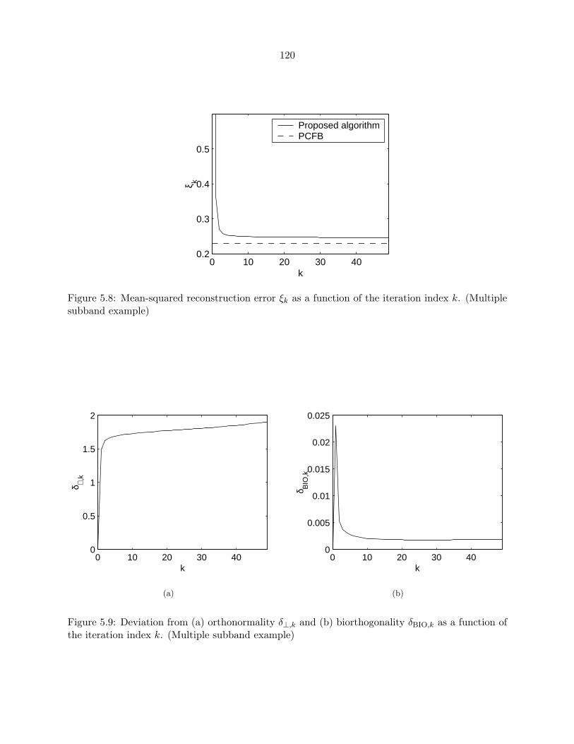
120

0 10 20 30 400.2

0.3

0.4

0.5

k

ξ k

Proposed algorithmPCFB

Figure 5.8: Mean-squared reconstruction error ξk as a function of the iteration index k. (Multiplesubband example)

0 10 20 30 400

0.5

1

1.5

2

k

δ ⊥,k

(a)

0 10 20 30 400

0.005

0.01

0.015

0.02

0.025

k

δ BIO

,k

(b)

Figure 5.9: Deviation from (a) orthonormality δ⊥,k and (b) biorthogonality δBIO,k as a function ofthe iteration index k. (Multiple subband example)

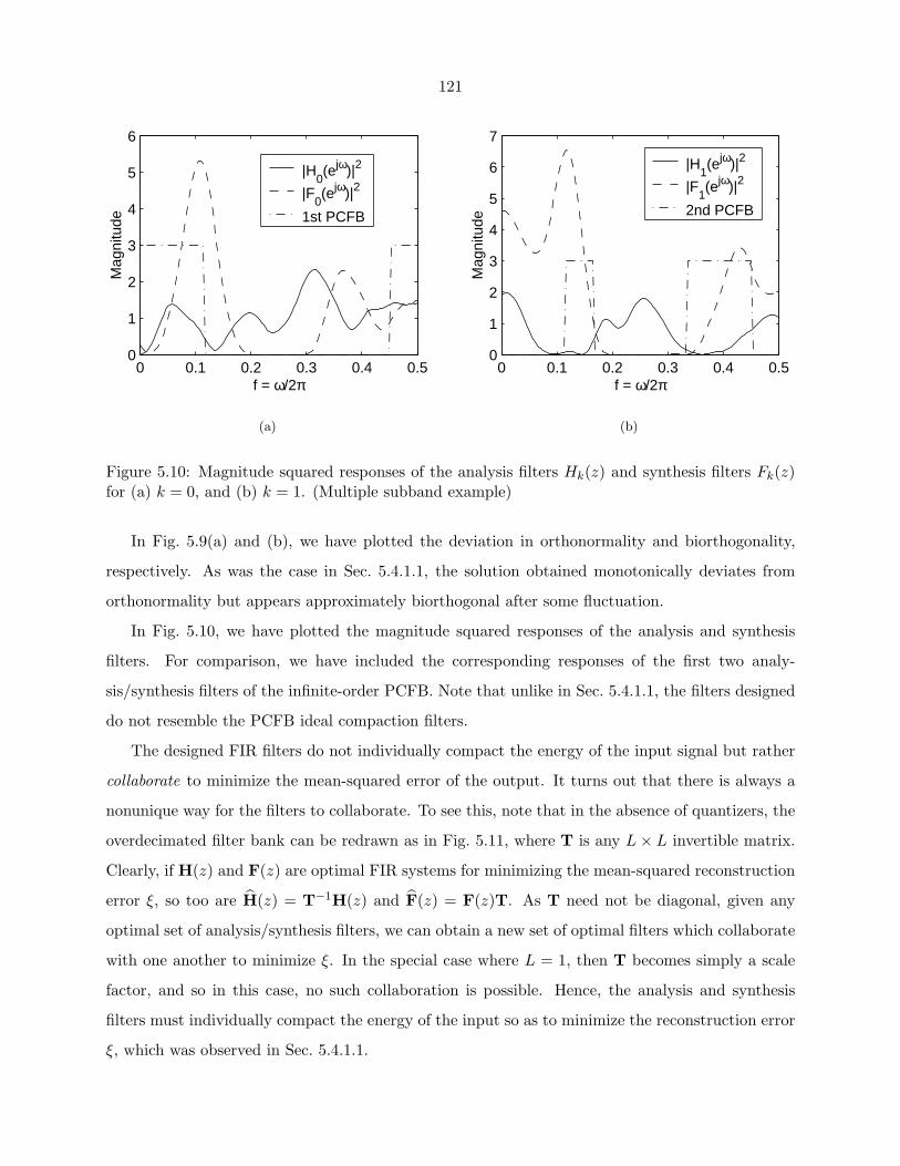
121

0 0.1 0.2 0.3 0.4 0.50

1

2

3

4

5

6

f = ω/2π

Mag

nitu

de

|H0(ejω)|2

|F0(ejω)|2

1st PCFB

(a)

0 0.1 0.2 0.3 0.4 0.50

1

2

3

4

5

6

7

f = ω/2π

Mag

nitu

de

|H1(ejω)|2

|F1(ejω)|2

2nd PCFB

(b)

Figure 5.10: Magnitude squared responses of the analysis filters Hk(z) and synthesis filters Fk(z)for (a) k = 0, and (b) k = 1. (Multiple subband example)

In Fig. 5.9(a) and (b), we have plotted the deviation in orthonormality and biorthogonality,

respectively. As was the case in Sec. 5.4.1.1, the solution obtained monotonically deviates from

orthonormality but appears approximately biorthogonal after some fluctuation.

In Fig. 5.10, we have plotted the magnitude squared responses of the analysis and synthesis

filters. For comparison, we have included the corresponding responses of the first two analy-

sis/synthesis filters of the infinite-order PCFB. Note that unlike in Sec. 5.4.1.1, the filters designed

do not resemble the PCFB ideal compaction filters.

The designed FIR filters do not individually compact the energy of the input signal but rather

collaborate to minimize the mean-squared error of the output. It turns out that there is always a

nonunique way for the filters to collaborate. To see this, note that in the absence of quantizers, the

overdecimated filter bank can be redrawn as in Fig. 5.11, where T is any L × L invertible matrix.

Clearly, if H(z) and F(z) are optimal FIR systems for minimizing the mean-squared reconstruction

error ξ, so too are H(z) = T−1H(z) and F(z) = F(z)T. As T need not be diagonal, given any

optimal set of analysis/synthesis filters, we can obtain a new set of optimal filters which collaborate

with one another to minimize ξ. In the special case where L = 1, then T becomes simply a scale

factor, and so in this case, no such collaboration is possible. Hence, the analysis and synthesis

filters must individually compact the energy of the input so as to minimize the reconstruction error

ξ, which was observed in Sec. 5.4.1.1.

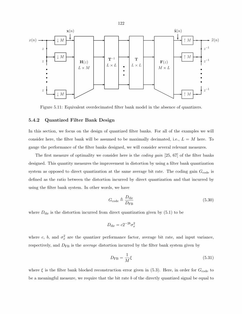
122

T

L × L

�

�

�

�

�

�

↑ M

↑ M

↑ M

�

�

�

�

z−1

z−1

z−1

x(n)

x(n)

�

F(z)

M × L

T−1

L × L

�

�

�

�

�

�

↓ M

↓ M

↓ M

�

�

�

�

�

�

� �

�

�

x(n)

z

z

z

x(n)

�

H(z)

L × M

Figure 5.11: Equivalent overdecimated filter bank model in the absence of quantizers.

5.4.2 Quantized Filter Bank Design

In this section, we focus on the design of quantized filter banks. For all of the examples we will

consider here, the filter bank will be assumed to be maximally decimated, i.e., L = M here. To

gauge the performance of the filter banks designed, we will consider several relevant measures.

The first measure of optimality we consider here is the coding gain [25, 67] of the filter banks

designed. This quantity measures the improvement in distortion by using a filter bank quantization

system as opposed to direct quantization at the same average bit rate. The coding gain Gcode is

defined as the ratio between the distortion incurred by direct quantization and that incurred by

using the filter bank system. In other words, we have

Gcode � Ddir

DFB(5.30)

where Ddir is the distortion incurred from direct quantization given by (5.1) to be

Ddir = c2−2bσ2x

where c, b, and σ2x are the quantizer performance factor, average bit rate, and input variance,

respectively, and DFB is the average distortion incurred by the filter bank system given by

DFB =1M

ξ (5.31)

where ξ is the filter bank blocked reconstruction error given in (5.3). Here, in order for Gcode to

be a meaningful measure, we require that the bit rate b of the directly quantized signal be equal to

123

the average bit rate of the filter bank quantization system, i.e., we have

b =1M

M−1∑k=0

bk (5.32)

Hence, the coding gain is a measure of the improvement in terms of distortion offered by using

a sophisticated filter bank quantization scheme as opposed to an unsophisticated single quantizer

system at the same bit rate.

In certain special cases, the coding gain can be simplified greatly. For example, if the quantized

filter bank system of Fig. 5.1 is a maximally decimated orthonormal or PU filter bank, the coding

gain becomes [25, 72]

Gcode =c2−2bσ2

x

1M

M−1∑k=0

σ2qk

=c2−2bσ2

x

1M

M−1∑k=0

ck2−2bkσ2wk

Assuming that all of the subband quantizer performance factors ck are all equal to c, which occurs

if the input pdfs are all the same, then we have

Gcode =2−2bσ2

x

1M

M−1∑k=0

2−2bkσ2wk

It turns out [25, 67] that for any fixed PU filter bank, there is an optimal way to allocate the

subband bit rates {bk} subject to the average bit rate constraint of (5.32) to maximize Gcode. This

occurs as a result of using the arithmetic mean/geometric mean (AM/GM) inequality [22, 67].

With optimal bit allocation, the coding gain becomes

Gcode =σ2

x(M−1∏k=0

σ2wk

) 1M

=

1M

M−1∑k=0

σ2wk(

M−1∏k=0

σ2wk

) 1M

which is itself the AM/GM ratio of the subband variances. By the AM/GM inequality, we always

have Gcode ≥ 1 and so for any PU filter bank, there is always an improvement in terms of distortion

if the bits have been optimally allocated. With optimal bit allocation, among all PU filter banks

of a certain class, the PCFB, if it exists, exhibits the largest coding gain [1, 68].

Using the proposed iterative greedy algorithm of this chapter, it can be seen from (5.30) and

(5.31) that we obtain a filter bank system whose coding gain is monotonic nondecreasing with

iteration for a fixed bit allocation {bk}. This is more practical than optimizing the bit allocation

for a fixed filter bank, which will often times yield unrealizable noninteger bit allocations [25, 67].

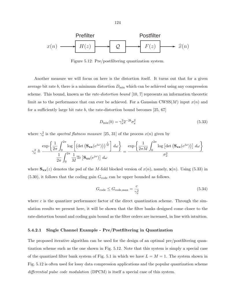
124

� H(z) � Q � F (z) �x(n)

Prefilter Postfilter

x(n)

Figure 5.12: Pre/postfiltering quantization system.

Another measure we will focus on here is the distortion itself. It turns out that for a given

average bit rate b, there is a minimum distortion Dmin which can be achieved using any compression

scheme. This bound, known as the rate-distortion bound [10, 7] represents an information theoretic

limit as to the performance that can ever be achieved. For a Gaussian CWSS(M) input x(n) and

for a sufficiently large bit rate b, the rate-distortion bound becomes [25, 67]

Dmin(b) = γ2x2−2bσ2

x (5.33)

where γ2x is the spectral flatness measure [25, 31] of the process x(n) given by

γ2x �

exp{

12π

∫ 2π

0log

[(det

(Sxx(ejω)

)) 1M

]dω

}12π

∫ 2π

0

1M

Tr[Sxx(ejω)

]dω

=exp

{1

2πM

∫ 2π

0log

[det

(Sxx(ejω)

)]dω

}σ2

x

where Sxx(z) denotes the psd of the M -fold blocked version of x(n), namely, x(n). Using (5.33) in

(5.30), it follows that the coding gain Gcode can be upper bounded as follows.

Gcode ≤ Gcode,max =c

γ2x

(5.34)

where c is the quantizer performance factor of the direct quantization scheme. Through the sim-

ulation results we present here, it will be shown that the filter banks designed come closer to the

rate-distortion bound and coding gain bound as the filter orders are increased, in line with intuition.

5.4.2.1 Single Channel Example - Pre/Postfiltering in Quantization

The proposed iterative algorithm can be used for the design of an optimal pre/postfiltering quan-

tization scheme such as the one shown in Fig. 5.12. Note that this system is simply a special case

of the quantized filter bank system of Fig. 5.1 in which we have L = M = 1. The system shown in

Fig. 5.12 is often used for lossy data compression applications and the popular quantization scheme

differential pulse code modulation (DPCM) is itself a special case of this system.

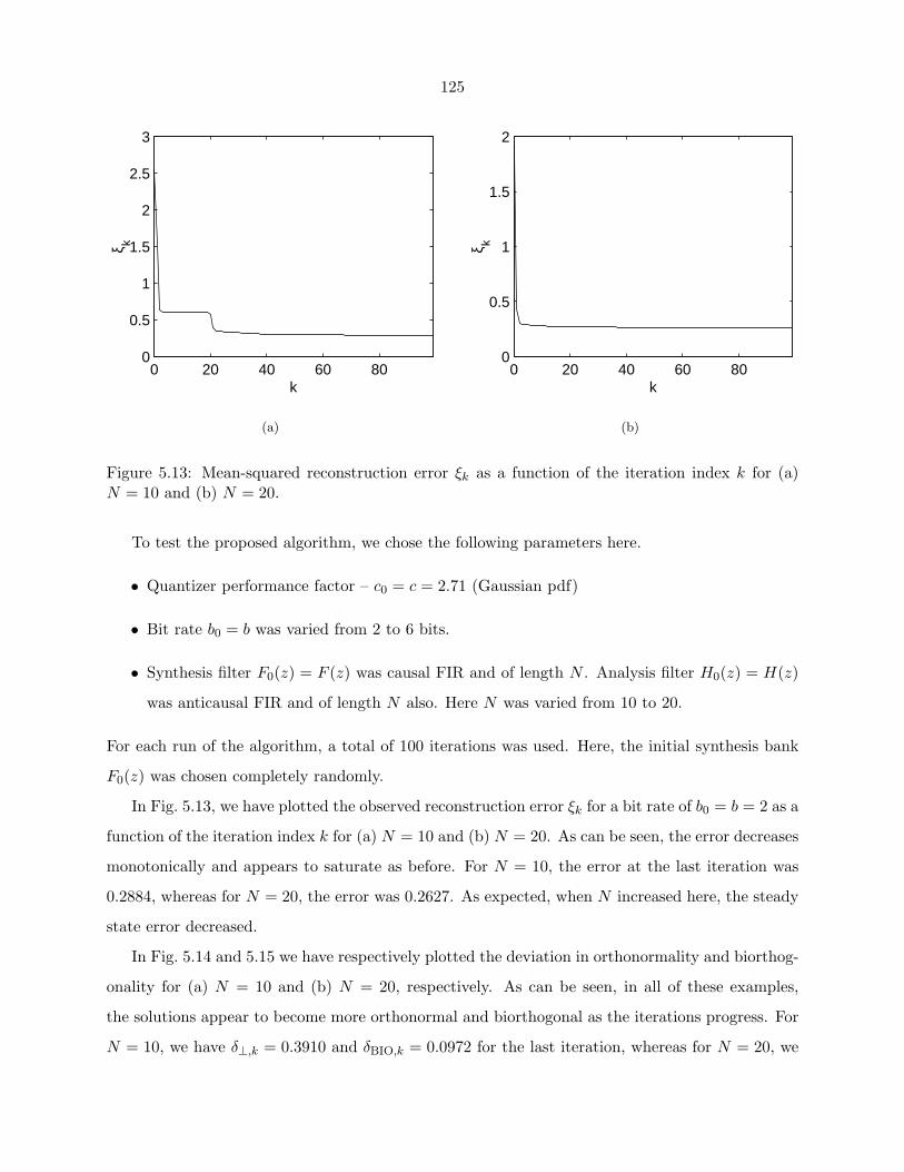
125

0 20 40 60 800

0.5

1

1.5

2

2.5

3

k

ξ k

(a)

0 20 40 60 800

0.5

1

1.5

2

k

ξ k

(b)

Figure 5.13: Mean-squared reconstruction error ξk as a function of the iteration index k for (a)N = 10 and (b) N = 20.

To test the proposed algorithm, we chose the following parameters here.

• Quantizer performance factor – c0 = c = 2.71 (Gaussian pdf)

• Bit rate b0 = b was varied from 2 to 6 bits.

• Synthesis filter F0(z) = F (z) was causal FIR and of length N . Analysis filter H0(z) = H(z)

was anticausal FIR and of length N also. Here N was varied from 10 to 20.

For each run of the algorithm, a total of 100 iterations was used. Here, the initial synthesis bank

F0(z) was chosen completely randomly.

In Fig. 5.13, we have plotted the observed reconstruction error ξk for a bit rate of b0 = b = 2 as a

function of the iteration index k for (a) N = 10 and (b) N = 20. As can be seen, the error decreases

monotonically and appears to saturate as before. For N = 10, the error at the last iteration was

0.2884, whereas for N = 20, the error was 0.2627. As expected, when N increased here, the steady

state error decreased.

In Fig. 5.14 and 5.15 we have respectively plotted the deviation in orthonormality and biorthog-

onality for (a) N = 10 and (b) N = 20, respectively. As can be seen, in all of these examples,

the solutions appear to become more orthonormal and biorthogonal as the iterations progress. For

N = 10, we have δ⊥,k = 0.3910 and δBIO,k = 0.0972 for the last iteration, whereas for N = 20, we

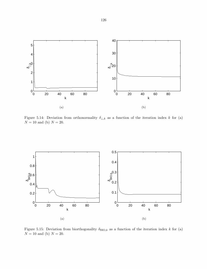
126

0 20 40 60 800

1

2

3

4

5

k

δ ⊥,k

(a)

0 20 40 60 800

10

20

30

40

k

δ ⊥,k

(b)

Figure 5.14: Deviation from orthonormality δ⊥,k as a function of the iteration index k for (a)N = 10 and (b) N = 20.

0 20 40 60 800

0.2

0.4

0.6

0.8

1

k

δ BIO

,k

(a)

0 20 40 60 800

0.1

0.2

0.3

0.4

0.5

k

δ BIO

,k

(b)

Figure 5.15: Deviation from biorthogonality δBIO,k as a function of the iteration index k for (a)N = 10 and (b) N = 20.

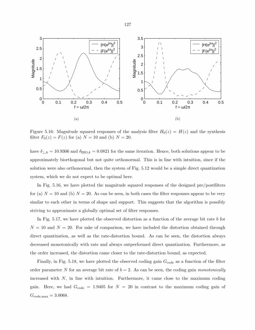
127

0 0.1 0.2 0.3 0.4 0.50

0.5

1

1.5

2

2.5

3

f = ω/2π

Mag

nitu

de

|H(ejω)|2

|F(ejω)|2

(a)

0 0.1 0.2 0.3 0.4 0.50

0.5

1

1.5

2

2.5

3

3.5

f = ω/2π

Mag

nitu

de

|H(ejω)|2

|F(ejω)|2

(b)

Figure 5.16: Magnitude squared responses of the analysis filter H0(z) = H(z) and the synthesisfilter F0(z) = F (z) for (a) N = 10 and (b) N = 20.

have δ⊥,k = 10.9306 and δBIO,k = 0.0821 for the same iteration. Hence, both solutions appear to be

approximately biorthogonal but not quite orthonormal. This is in line with intuition, since if the

solution were also orthonormal, then the system of Fig. 5.12 would be a simple direct quantization

system, which we do not expect to be optimal here.

In Fig. 5.16, we have plotted the magnitude squared responses of the designed pre/postfilters

for (a) N = 10 and (b) N = 20. As can be seen, in both cases the filter responses appear to be very

similar to each other in terms of shape and support. This suggests that the algorithm is possibly

striving to approximate a globally optimal set of filter responses.

In Fig. 5.17, we have plotted the observed distortion as a function of the average bit rate b for

N = 10 and N = 20. For sake of comparison, we have included the distortion obtained through

direct quantization, as well as the rate-distortion bound. As can be seen, the distortion always

decreased monotonically with rate and always outperformed direct quantization. Furthermore, as

the order increased, the distortion came closer to the rate-distortion bound, as expected.

Finally, in Fig. 5.18, we have plotted the observed coding gain Gcode as a function of the filter

order parameter N for an average bit rate of b = 2. As can be seen, the coding gain monotonically

increased with N , in line with intuition. Furthermore, it came close to the maximum coding

gain. Here, we had Gcode = 1.9405 for N = 20 in contrast to the maximum coding gain of

Gcode,max = 3.0068.

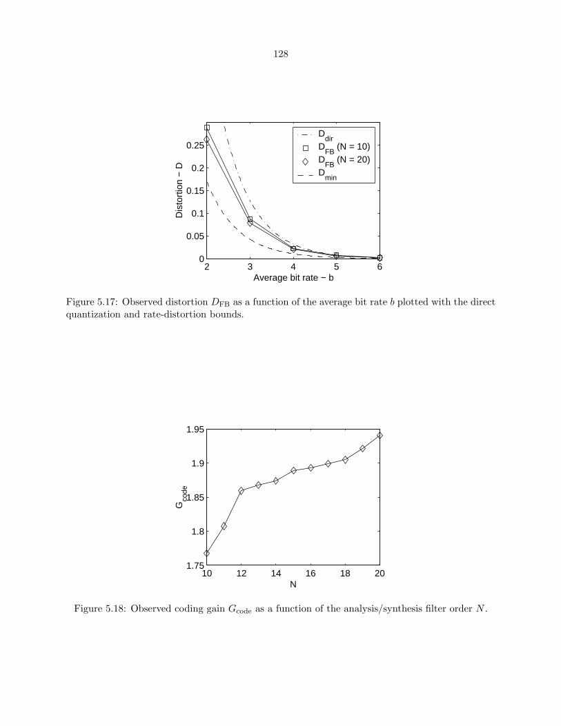
128

2 3 4 5 60

0.05

0.1

0.15

0.2

0.25

Average bit rate − b

Dis

tort

ion

− D

Ddir

DFB

(N = 10)D

FB (N = 20)

Dmin

Figure 5.17: Observed distortion DFB as a function of the average bit rate b plotted with the directquantization and rate-distortion bounds.

10 12 14 16 18 201.75

1.8

1.85

1.9

1.95

N

Gco

de

Figure 5.18: Observed coding gain Gcode as a function of the analysis/synthesis filter order N .

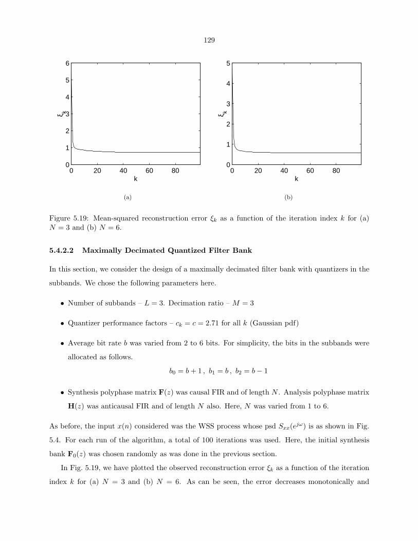
129

0 20 40 60 800

1

2

3

4

5

6

k

ξ k

(a)

0 20 40 60 800

1

2

3

4

5

k

ξ k

(b)

Figure 5.19: Mean-squared reconstruction error ξk as a function of the iteration index k for (a)N = 3 and (b) N = 6.

5.4.2.2 Maximally Decimated Quantized Filter Bank

In this section, we consider the design of a maximally decimated filter bank with quantizers in the

subbands. We chose the following parameters here.

• Number of subbands – L = 3. Decimation ratio – M = 3

• Quantizer performance factors – ck = c = 2.71 for all k (Gaussian pdf)

• Average bit rate b was varied from 2 to 6 bits. For simplicity, the bits in the subbands were

allocated as follows.

b0 = b + 1 , b1 = b , b2 = b − 1

• Synthesis polyphase matrix F(z) was causal FIR and of length N . Analysis polyphase matrix

H(z) was anticausal FIR and of length N also. Here, N was varied from 1 to 6.

As before, the input x(n) considered was the WSS process whose psd Sxx(ejω) is as shown in Fig.

5.4. For each run of the algorithm, a total of 100 iterations was used. Here, the initial synthesis

bank F0(z) was chosen randomly as was done in the previous section.

In Fig. 5.19, we have plotted the observed reconstruction error ξk as a function of the iteration

index k for (a) N = 3 and (b) N = 6. As can be seen, the error decreases monotonically and

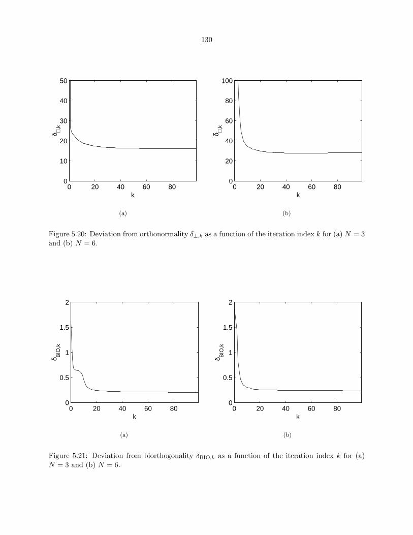
130

0 20 40 60 800

10

20

30

40

50

k

δ ⊥,k

(a)

0 20 40 60 800

20

40

60

80

100

k

δ ⊥,k

(b)

Figure 5.20: Deviation from orthonormality δ⊥,k as a function of the iteration index k for (a) N = 3and (b) N = 6.

0 20 40 60 800

0.5

1

1.5

2

k

δ BIO

,k

(a)

0 20 40 60 800

0.5

1

1.5

2

k

δ BIO

,k

(b)

Figure 5.21: Deviation from biorthogonality δBIO,k as a function of the iteration index k for (a)N = 3 and (b) N = 6.

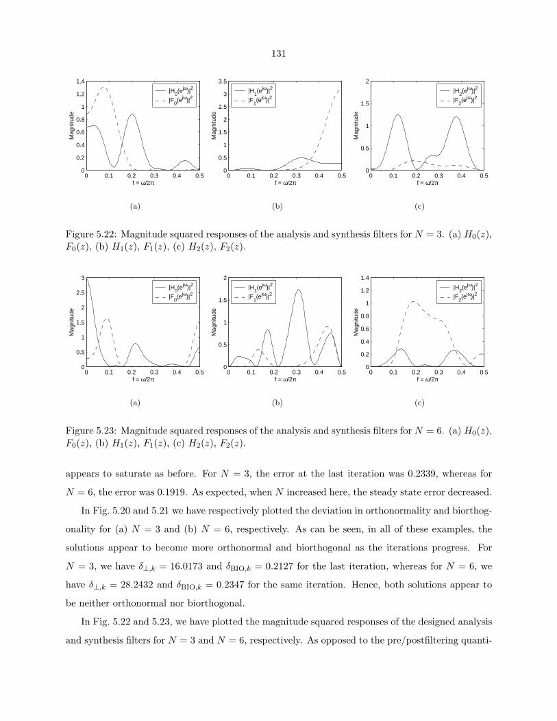
131

0 0.1 0.2 0.3 0.4 0.50

0.2

0.4

0.6

0.8

1

1.2

1.4

f = ω/2π

Mag

nitu

de

|H0(ejω)|2

|F0(ejω)|2

(a)

0 0.1 0.2 0.3 0.4 0.50

0.5

1

1.5

2

2.5

3

3.5

f = ω/2π

Mag

nitu

de

|H1(ejω)|2

|F1(ejω)|2

(b)

0 0.1 0.2 0.3 0.4 0.50

0.5

1

1.5

2

f = ω/2π

Mag

nitu

de

|H2(ejω)|2

|F2(ejω)|2

(c)

Figure 5.22: Magnitude squared responses of the analysis and synthesis filters for N = 3. (a) H0(z),F0(z), (b) H1(z), F1(z), (c) H2(z), F2(z).

0 0.1 0.2 0.3 0.4 0.50

0.5

1

1.5

2

2.5

3

f = ω/2π

Mag

nitu

de

|H0(ejω)|2

|F0(ejω)|2

(a)

0 0.1 0.2 0.3 0.4 0.50

0.5

1

1.5

2

f = ω/2π

Mag

nitu

de

|H1(ejω)|2

|F1(ejω)|2

(b)

0 0.1 0.2 0.3 0.4 0.50

0.2

0.4

0.6

0.8

1

1.2

1.4

f = ω/2π

Mag

nitu

de

|H2(ejω)|2

|F2(ejω)|2

(c)

Figure 5.23: Magnitude squared responses of the analysis and synthesis filters for N = 6. (a) H0(z),F0(z), (b) H1(z), F1(z), (c) H2(z), F2(z).

appears to saturate as before. For N = 3, the error at the last iteration was 0.2339, whereas for

N = 6, the error was 0.1919. As expected, when N increased here, the steady state error decreased.

In Fig. 5.20 and 5.21 we have respectively plotted the deviation in orthonormality and biorthog-

onality for (a) N = 3 and (b) N = 6, respectively. As can be seen, in all of these examples, the

solutions appear to become more orthonormal and biorthogonal as the iterations progress. For

N = 3, we have δ⊥,k = 16.0173 and δBIO,k = 0.2127 for the last iteration, whereas for N = 6, we

have δ⊥,k = 28.2432 and δBIO,k = 0.2347 for the same iteration. Hence, both solutions appear to

be neither orthonormal nor biorthogonal.

In Fig. 5.22 and 5.23, we have plotted the magnitude squared responses of the designed analysis

and synthesis filters for N = 3 and N = 6, respectively. As opposed to the pre/postfiltering quanti-

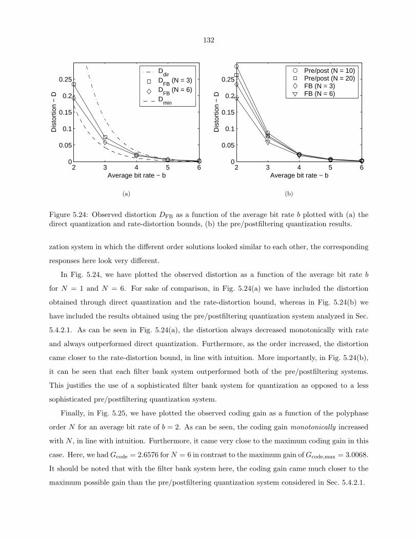
132

2 3 4 5 60

0.05

0.1

0.15

0.2

0.25

Average bit rate − b

Dis

tort

ion

− D

Ddir

DFB

(N = 3)D

FB (N = 6)

Dmin

(a)

2 3 4 5 60

0.05

0.1

0.15

0.2

0.25

Average bit rate − b

Dis

tort

ion

− D

Pre/post (N = 10)Pre/post (N = 20)FB (N = 3)FB (N = 6)

(b)

Figure 5.24: Observed distortion DFB as a function of the average bit rate b plotted with (a) thedirect quantization and rate-distortion bounds, (b) the pre/postfiltering quantization results.

zation system in which the different order solutions looked similar to each other, the corresponding

responses here look very different.

In Fig. 5.24, we have plotted the observed distortion as a function of the average bit rate b

for N = 1 and N = 6. For sake of comparison, in Fig. 5.24(a) we have included the distortion

obtained through direct quantization and the rate-distortion bound, whereas in Fig. 5.24(b) we

have included the results obtained using the pre/postfiltering quantization system analyzed in Sec.

5.4.2.1. As can be seen in Fig. 5.24(a), the distortion always decreased monotonically with rate

and always outperformed direct quantization. Furthermore, as the order increased, the distortion

came closer to the rate-distortion bound, in line with intuition. More importantly, in Fig. 5.24(b),

it can be seen that each filter bank system outperformed both of the pre/postfiltering systems.

This justifies the use of a sophisticated filter bank system for quantization as opposed to a less

sophisticated pre/postfiltering quantization system.

Finally, in Fig. 5.25, we have plotted the observed coding gain as a function of the polyphase

order N for an average bit rate of b = 2. As can be seen, the coding gain monotonically increased

with N , in line with intuition. Furthermore, it came very close to the maximum coding gain in this

case. Here, we had Gcode = 2.6576 for N = 6 in contrast to the maximum gain of Gcode,max = 3.0068.

It should be noted that with the filter bank system here, the coding gain came much closer to the

maximum possible gain than the pre/postfiltering quantization system considered in Sec. 5.4.2.1.

133

1 2 3 4 5 61

1.5

2

2.5

3

N

Gco

de

Figure 5.25: Observed coding gain Gcode as a function of the analysis/synthesis polyphase filterorder N .

5.5 Concluding Remarks

In this chapter, we presented a method for the design of purely FIR filter banks for optimal

reconstruction with the presence of scalar quantizers in the subbands. Under the high bit rate

assumption for the quantizers [25], we showed that the mean-squared error objective was quadratic

in terms of either the analysis or synthesis filter coefficients and hence could be minimized using

the trick of completing the square [22]. By alternately optimizing the analysis and synthesis banks,

we proposed an iterative greedy algorithm for the design of such FIR filter banks.

Simulation results presented here brought to light the merit of the proposed iterative algorithm.

We showed how the algorithm could be used to obtain minimum mean-squared error overdecimated

filter banks. In addition, we showed that sometimes the filter banks designed exhibited behavior

similar to the ideal compaction filters of the PCFB.

Afterwards, we focused on the effects of quantization and used the algorithm to design pre/post-

filtering quantization schemes as well as general filter bank quantization systems. It was shown

that in terms of coding gain and distortion, the systems designed came close to the theoretical

bounds established by information theory. In line with intuition, we showed that as the filter order

increased, the quantization systems monotonically came closer to these bounds. Furthermore,

we showed the advantages of using a sophisticated filter bank quantization system over a simple

pre/postfiltering quantization scheme. In particular, it was observed that the filter bank system

could come much closer to the optimal information theoretic bounds than the pre/postfiltering

system. These phenomena have not previously been formally presented in the literature.

134

Chapter 6

Eigenfilter Channel ShorteningEqualizer for DMT Systems

In this chapter, we show how the eigenfilter technique [74, 56], which was widely used in the

optimization algorithms presented for designing signal-adapted filter banks, can be applied to the

design of good channel shortening equalizers for discrete multitone (DMT) systems. This chapter

differs in theme from the others in that the optimization algorithm is not iterative as the equalizer

is designed in one step. The design objective we focus on here takes into account both the effects

due to the channel length as well as the noise. We show how our method can be used for the design

of fractionally spaced equalizers (FSEs). In contrast to other methods which require a Cholesky

decomposition of a certain matrix for every delay parameter chosen, the method presented here

only requires one such decomposition, as we show here. As such, this method is lower in complexity

than those mentioned above. Despite this decrease in complexity, we show that the method yields

nearly optimal performance in terms of bit rate or throughput.

The content of this chapter is mainly drawn from [55] and portions of it have been presented

at [53, 51, 52].

6.1 Outline

In Sec. 6.2, we briefly review the channel shortening equalizer design problem and how it relates

to DMT systems. A survey of some of the previous work related to the design of such equalizers is

given in Sec. 6.2.1.

135

� C(z) � � H(z) �

x(n)

Channel Equalizer

y(n)

η(n)

Noise

Figure 6.1: Channel shortening equalizer model.

In Sec. 6.3, we introduce the design objective that we will focus on here. The objective consid-

ered jointly accounts for the channel shortening objective, as well as the effects due to noise. In

Sec. 6.3.1, we analyze the objective function and show how it can be solved using the eigenfilter

approach. There, the low complexity advantage of the proposed method is revealed.

In Sec. 6.4, we present simulation results for the proposed channel shortening equalizer design

method, along with those of several other methods. There, it is shown that the method outperforms

most methods and performs nearly optimally in terms of observed bit rate.

Concluding remarks are made in Sec. 6.5. In the Appendix, we show the equivalence between

FSEs and the SIMO-MISO channel/equalizer model we focus on in Sec. 6.3.

6.2 The Channel Shortening Equalizer Problem

Suppose that we have a causal FIR system or channel C(z) of length Lc that we would like to

shorten to a length Ld < Lc. A typical model for the system used to shorten the channel is shown

in Fig. 6.1. The goal of the equalizer H(z) is to shorten the effective channel Ceff(z) � H(z)C(z) to

a length of Ld. Though this can be done exactly by choosing H(z) = A(z)C(z) , where A(z) is some FIR

system of length Ld, there are often problems with this approach. As C(z) may have zeros on or

outside the unit circle, the choice of H(z) = A(z)C(z) , which we assume must be causal here, can never

be stable. This in turn will result in the undesired phenomenon of spurious noise amplification.

Instead, what is typically done is to choose H(z) to be a causal FIR filter used to concentrate

the energy of the effective channel Ceff(z) into a window of length Ld. If H(z) is of length Le,

then Ceff(z) = H(z)C(z) is a causal FIR system of length Leff � (Lc + Le − 1). In this case, we

can decompose the effective channel impulse response ceff(n) as a sum of two responses, namely, a

desired response cdes(n) which is exactly of length Ld, and a residual response cres(n) which consists

of whatever remains of ceff(n) after removing cdes(n). This is illustrated in Fig. 6.2. Here, ∆ is

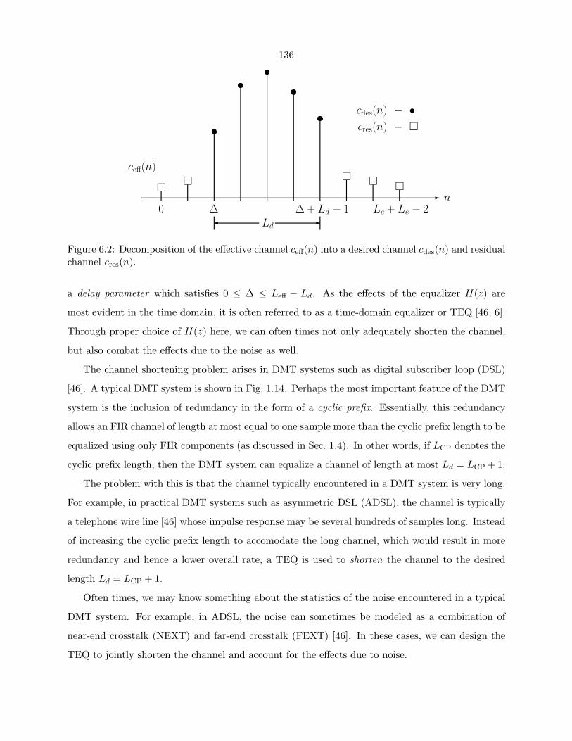
136

�� � � � �

ceff(n)

0 ∆ ∆ + Ld − 1� �Ld

Lc + Le − 2n

cdes(n) − •cres(n) − �

Figure 6.2: Decomposition of the effective channel ceff(n) into a desired channel cdes(n) and residualchannel cres(n).

a delay parameter which satisfies 0 ≤ ∆ ≤ Leff − Ld. As the effects of the equalizer H(z) are

most evident in the time domain, it is often referred to as a time-domain equalizer or TEQ [46, 6].

Through proper choice of H(z) here, we can often times not only adequately shorten the channel,

but also combat the effects due to the noise as well.

The channel shortening problem arises in DMT systems such as digital subscriber loop (DSL)

[46]. A typical DMT system is shown in Fig. 1.14. Perhaps the most important feature of the DMT

system is the inclusion of redundancy in the form of a cyclic prefix. Essentially, this redundancy

allows an FIR channel of length at most equal to one sample more than the cyclic prefix length to be

equalized using only FIR components (as discussed in Sec. 1.4). In other words, if LCP denotes the

cyclic prefix length, then the DMT system can equalize a channel of length at most Ld = LCP + 1.

The problem with this is that the channel typically encountered in a DMT system is very long.

For example, in practical DMT systems such as asymmetric DSL (ADSL), the channel is typically

a telephone wire line [46] whose impulse response may be several hundreds of samples long. Instead

of increasing the cyclic prefix length to accomodate the long channel, which would result in more

redundancy and hence a lower overall rate, a TEQ is used to shorten the channel to the desired

length Ld = LCP + 1.

Often times, we may know something about the statistics of the noise encountered in a typical

DMT system. For example, in ADSL, the noise can sometimes be modeled as a combination of

near-end crosstalk (NEXT) and far-end crosstalk (FEXT) [46]. In these cases, we can design the

TEQ to jointly shorten the channel and account for the effects due to noise.

137

For a DMT system, the primary measure of optimality of a TEQ is the overall bit rate or

throughput of the system. This measure accounts for both the effects due to the channel length as

well as the noise. If fs denotes the analog sampling frequency and NDFT denotes the size of the

DFT matrix used in the DMT system (see Fig. 1.14), then the observed bit rate is given by [6]

Rb =fs

NDFT + LCP

∑k∈S

bk (6.1)

where bk denotes the number of bits to allocate for the k-th real subcarrier and S is a subset of the

set of real subcarriers{

0, 1, . . . , NDFT2 − 1

}that are used. Here, S is chosen according to the famous

“water filling” principle [10, 7], as the subcarriers are modeled as parallel independent Gaussian

channels [46]. As such, the number of bits to allocate for the k-th subcarrier is [6]

bk = log2

(1 +

SNRk

Γ

)where SNRk is the signal-to-noise (SNR) ratio for the k-th subcarrier which takes into account the

effects due to both the channel length and the noise given by

SNRk =Sxx(ejωk)

∣∣Cdes(ejωk)∣∣2

Sxx(ejωk) |Cres(ejωk)|2 + Sηη(ejωk) |H(ejωk)|2 , where ωk =2πk

NDFT

and Γ is an SNR gap [46] for achieving the Shannon capacity limit [10, 7] that is assumed to be the

same for all subcarriers. Also, Sxx(ejω) and Sηη(ejω) denote, respectively, the psds of the input to

the channel and noise (see Fig. 6.1), which we have assumed are WSS here. The quantity Γ depends

on the modulation format used as well as the desired probability of error [46, 6]. For uncoded

quadrature amplitude modulation (QAM) [38] with a probability of error of 10−7, Γ = 9.8 dB [46].

The maximum achievable bit rate is given by the matched-filter bound (MFB) [6], which is

RMFB =fs

NDFT + LCP

∑k∈S

bk (6.2)

where bk is the number of bits allocated to the k-th subcarrier given by

bk = log2

(1 +

SNRMFB,k

Γ

)and SNRMFB,k is the MFB SNR given by

SNRMFB,k =Sxx(ejωk)

∣∣C(ejωk)∣∣2

Sηη(ejωk), ωk =

2πk

NDFT

Note that the MFB SNR is only a function of the statistics of the input and noise, as well as the

channel response. These are the only invariants of the communications system and as such, dictate

the maximum possible performance alone.

Prior to presenting our method for TEQ design, we briefly review previous work on the matter.

138

6.2.1 Overview of Previous Work on Channel Shortening Equalizers

1. Minimum Mean-Squared Error (MMSE) Methods: Among the first approaches for the design

of channel shortening equalizers were the minimum mean-squared error (MMSE) methods

proposed by Al-Dhahir and Cioffi [3, 4]. With these methods, the TEQ h(n) is chosen to be

an FIR Wiener filter [48] for the response b(n) ∗ x(n), where b(n) is a target impulse response

(TIR), which is some FIR system of length Ld. In other words, referring to Fig. 6.1, the

equalizer h(n) is chosen to minimize

ξ � E[|y(n) − b(n) ∗ x(n)|2

]For a fixed TIR b(n), the TEQ coefficients of h(n) can be found using the orthogonality

principle [48].

Early methods for the design of the TIR b(n) consisted of choosing it such that b(n) satisfied

a unit energy or unit tap constraint as shown below [3].∑n

|b(n)|2 = 1 (Unit Energy Constraint (UEC))

b(n0) = 1 for some n0 (Unit Tap Constraint (UTC))

Though these choices of b(n) are easy to obtain and compute, they often perform poorly with

respect to overall observed bit rate. Furthermore, once b(n) has been appropriately computed,

the equalizer coefficients of h(n) must still be found using the orthogonality principle.

Another method for the design of the TIR b(n) perhaps better suited for DMT systems is the

geometric SNR (GSNR) method of [4]. In it, the authors obtained an approximate expression

for the bit rate and found that increasing the product of∣∣B(ejω)

∣∣2 at the DFT frequencies

ωk = 2πkNDFT

would increase the bit rate. Formally, the GSNR method consists of maximizing

this product, which is equivalent to maximizing the geometric mean of∣∣B(ejω)

∣∣2 at the DFT

frequencies, subject to a mean-squared error constraint ξ ≤ ξmax for some error threshold

value ξmax.

Unfortunately, the GSNR method suffers from several shortcomings. First of all, in their

expression for the bit rate, the authors of [4] did not take into account the effects due to

intersymbol interference (ISI) (i.e., the effects due to the channel length). Furthermore, they

treated the target response B(ejω) and equalizer H(ejω) as independent quantities, when in

fact h(n) is related to b(n) via the orthogonality principle. Finally, finding the TIR b(n)

139

involves solving a constrained nonlinear optimization problem, and as such, is very high in

computational complexity. Though the GSNR method often outperforms the UEC and UTC

methods of [3], other methods developed later not only surpass it, but also do so with less

computational complexity. Despite this, the GSNR method represented the first attempt to

design a TEQ by maximizing the bit rate of a DMT system.

2. Minimum Shortening SNR (MSSNR) Method: In [33], Melsa, Younce, and Rohrs developed

a method for designing a channel shortening equalizer that delt directly with the TEQ coef-

ficients of h(n). The objective was to maximize the shortening SNR (SSNR) given by

SSNR � Edes

Eres

where Edes and Eres denote, respectively, the energy of the effective desired response cdes(n)

and residual response cres(n) (see Fig. 6.2), given by

Edes =∑

n

|cdes(n)|2 , Eres =∑

n

|cres(n)|2

To maximize the SSNR, the authors of [33] solved the constrained optimization problem

Minimize Eres, subject to Edes = 1.

They showed that this optimization problem could be solved using the eigenfilter technique

[74, 56], after computing an appropriate Cholesky decomposition [22] of a particular matrix.

Though this method performs relatively well with relatively low complexity, on account of

the fact that the design problem is an eigenfilter-type problem, it suffers from several short-

comings. First, the method does not account for any effects due to noise present in the

system. Furthermore, the Cholesky factor obtained from the above-mentioned Cholesky de-

composition depends on the delay parameter ∆. If we wish to vary ∆ over a certain region to

see which value performs the best, which is typically done in practice, then a new Cholesky

factor must be computed for each ∆. This results in an extra computational load for each

∆ considered. Despite these shortcomings, the MSSNR method of [33] represented the first

attempt to pose the channel shortening problem as an eigenfilter-type problem.

3. Maximum Bit Rate (MBR) and Minimum ISI (Min-ISI) Methods: Arslan, Evans, and Kiaei

[6] were the first to design a TEQ to directly maximize the bit rate given in (6.1). This

method, called the maximum bit rate (MBR) method, was shown to perform very well and

140

often came very close to the MFB maximum achievable bit rate given in (6.2). However, as

the bit rate given in (6.1) is a nonlinear, nonconvex function of the TEQ coefficients of h(n),

computationally intensive nonlinear optimization techniques had to be employed to maximize

the bit rate. Furthermore, these techniques were found to converge slowly to a desired local

extrema.

In order to mitigate the effects of this complexity, the authors of [6] proposed a suboptimal

method called the minimum ISI (min-ISI) method in which the objective was to minimize

a combination of the effects due to ISI as well as those due to noise. As with the MSSNR

method of [33], it was shown that the objective could be optimized using the eigenfilter

approach after an appropriate Cholesky factor was computed. This method, as it accounted

for both ISI and noise, was shown to perform nearly as well as the MBR method with much

lower computational complexity. However, as with the MSSNR method of [33], the Cholesky

factor needed in the min-ISI method of [6] depends on the delay parameter ∆.

4. Delay Spread Minimization Method: Schur and Speidel proposed a unique method for the

design of channel shortening equalizers in [44]. In it, the objective was to minimize the delay

spread of the effective channel ceff(n), defined as follows.

Jdelay �

∑n

(n − ∆)2 |ceff(n)|2∑n

|ceff(n)|2

As with the MSSNR method of [33] and the min-ISI method of [6], it was shown that this

problem could be solved using the eigenfilter approach after an appropriate Cholesky factor

was computed. However, unlike these methods, the Cholesky factor required for the delay

spread minimization method does not depend on the delay parameter ∆. Hence, the method

is very low in complexity as only one Cholesky factor must be computed for all ∆.

Despite this significant decrease in complexity, the method suffers from several shortcomings.

Though the method was shown to be less prone to synchronization errors than others, it

does not account for the desired channel length Ld = LCP + 1 or any knowledge of the noise

statistics. Here, we generalize the delay spread minimization method of [44] to account for

both of these things. Furthermore, we apply it to a more general model than that shown in

Fig. 6.1 which can be used for the design of FSEs for channel shortening.

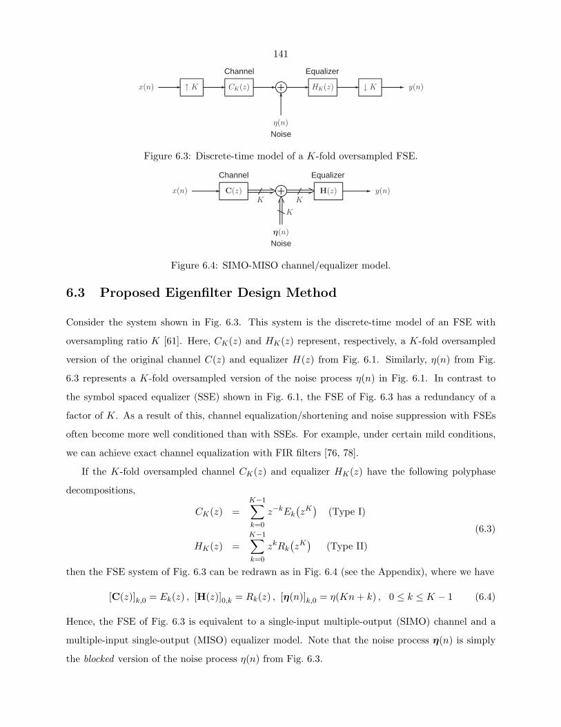
141

� ↑ K � CK(z) � � HK(z) � ↓ K �

x(n)

Channel Equalizer

y(n)

η(n)

Noise

Figure 6.3: Discrete-time model of a K-fold oversampled FSE.

� C(z)K

K

KH(z) �x(n)

Channel Equalizer

y(n)

η(n)

Noise

Figure 6.4: SIMO-MISO channel/equalizer model.

6.3 Proposed Eigenfilter Design Method

Consider the system shown in Fig. 6.3. This system is the discrete-time model of an FSE with

oversampling ratio K [61]. Here, CK(z) and HK(z) represent, respectively, a K-fold oversampled

version of the original channel C(z) and equalizer H(z) from Fig. 6.1. Similarly, η(n) from Fig.

6.3 represents a K-fold oversampled version of the noise process η(n) in Fig. 6.1. In contrast to

the symbol spaced equalizer (SSE) shown in Fig. 6.1, the FSE of Fig. 6.3 has a redundancy of a

factor of K. As a result of this, channel equalization/shortening and noise suppression with FSEs

often become more well conditioned than with SSEs. For example, under certain mild conditions,

we can achieve exact channel equalization with FIR filters [76, 78].

If the K-fold oversampled channel CK(z) and equalizer HK(z) have the following polyphase

decompositions,

CK(z) =K−1∑k=0

z−kEk

(zK)

(Type I)

HK(z) =K−1∑k=0

zkRk

(zK)

(Type II)

(6.3)

then the FSE system of Fig. 6.3 can be redrawn as in Fig. 6.4 (see the Appendix), where we have

[C(z)]k,0 = Ek(z) , [H(z)]0,k = Rk(z) , [η(n)]k,0 = η(Kn + k) , 0 ≤ k ≤ K − 1 (6.4)

Hence, the FSE of Fig. 6.3 is equivalent to a single-input multiple-output (SIMO) channel and a

multiple-input single-output (MISO) equalizer model. Note that the noise process η(n) is simply

the blocked version of the noise process η(n) from Fig. 6.3.

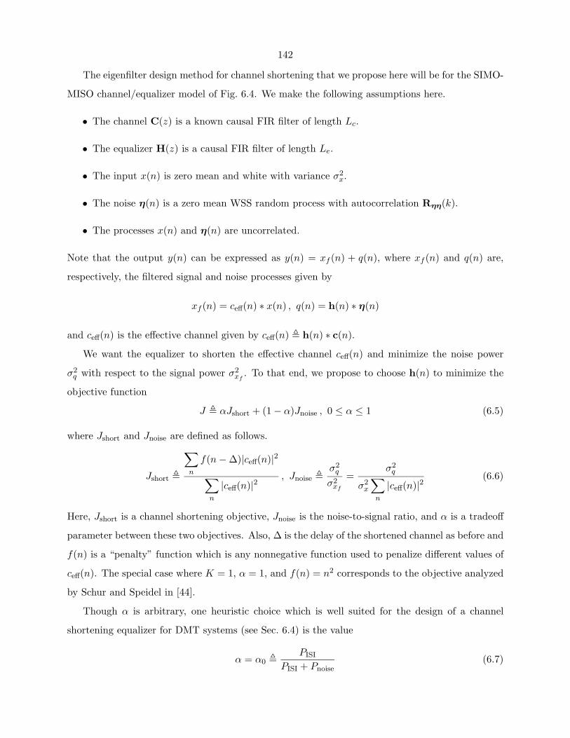
142

The eigenfilter design method for channel shortening that we propose here will be for the SIMO-

MISO channel/equalizer model of Fig. 6.4. We make the following assumptions here.

• The channel C(z) is a known causal FIR filter of length Lc.

• The equalizer H(z) is a causal FIR filter of length Le.

• The input x(n) is zero mean and white with variance σ2x.

• The noise η(n) is a zero mean WSS random process with autocorrelation Rηη(k).

• The processes x(n) and η(n) are uncorrelated.

Note that the output y(n) can be expressed as y(n) = xf (n) + q(n), where xf (n) and q(n) are,

respectively, the filtered signal and noise processes given by

xf (n) = ceff(n) ∗ x(n) , q(n) = h(n) ∗ η(n)

and ceff(n) is the effective channel given by ceff(n) � h(n) ∗ c(n).

We want the equalizer to shorten the effective channel ceff(n) and minimize the noise power

σ2q with respect to the signal power σ2

xf. To that end, we propose to choose h(n) to minimize the

objective function

J � αJshort + (1 − α)Jnoise , 0 ≤ α ≤ 1 (6.5)

where Jshort and Jnoise are defined as follows.

Jshort �

∑n

f(n − ∆)|ceff(n)|2∑n

|ceff(n)|2, Jnoise �

σ2q

σ2xf

=σ2

q

σ2x

∑n

|ceff(n)|2(6.6)

Here, Jshort is a channel shortening objective, Jnoise is the noise-to-signal ratio, and α is a tradeoff

parameter between these two objectives. Also, ∆ is the delay of the shortened channel as before and

f(n) is a “penalty” function which is any nonnegative function used to penalize different values of

ceff(n). The special case where K = 1, α = 1, and f(n) = n2 corresponds to the objective analyzed

by Schur and Speidel in [44].

Though α is arbitrary, one heuristic choice which is well suited for the design of a channel

shortening equalizer for DMT systems (see Sec. 6.4) is the value

α = α0 � PISI

PISI + Pnoise(6.7)

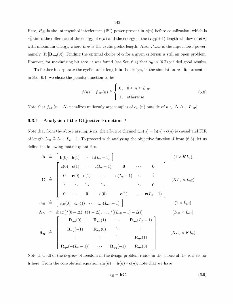
143

Here, PISI is the intersymbol interference (ISI) power present in c(n) before equalization, which is

σ2x times the difference of the energy of c(n) and the energy of the (LCP +1) length window of c(n)

with maximum energy, where LCP is the cyclic prefix length. Also, Pnoise is the input noise power,

namely, Tr [Rηη(0)]. Finding the optimal choice of α for a given criterion is still an open problem.

However, for maximizing bit rate, it was found (see Sec. 6.4) that α0 in (6.7) yielded good results.

To further incorporate the cyclic prefix length in the design, in the simulation results presented

in Sec. 6.4, we chose the penalty function to be

f(n) = fCP(n) �

0 , 0 ≤ n ≤ LCP

1 , otherwise(6.8)

Note that fCP(n − ∆) penalizes uniformly any samples of ceff(n) outside of n ∈ [∆, ∆ + LCP].

6.3.1 Analysis of the Objective Function J

Note that from the above assumptions, the effective channel ceff(n) = h(n)∗c(n) is causal and FIR

of length Leff � Lc + Le − 1. To proceed with analyzing the objective function J from (6.5), let us

define the following matrix quantities.

h �[

h(0) h(1) · · · h(Le − 1)]

(1 × KLe)

C �

c(0) c(1) · · · c(Lc − 1) 0 · · · 0

0 c(0) c(1) · · · c(Lc − 1). . .

......

. . . . . . . . . . . . 0

0 · · · 0 c(0) c(1) · · · c(Lc − 1)

(KLe × Leff)

ceff �[

ceff(0) ceff(1) · · · ceff(Leff − 1)]

(1 × Leff)

Λ∆ � diag (f(0 − ∆), f(1 − ∆), . . . , f((Leff − 1) − ∆)) (Leff × Leff)

Rη �

Rηη(0) Rηη(1) · · · Rηη(Le − 1)

Rηη(−1) Rηη(0). . .

......

. . . . . . Rηη(1)

Rηη(−(Le − 1)) · · · Rηη(−1) Rηη(0)

(KLe × KLe)

Note that all of the degrees of freedom in the design problem reside in the choice of the row vector

h here. From the convolution equation ceff(n) = h(n) ∗ c(n), note that we have

ceff = hC (6.9)

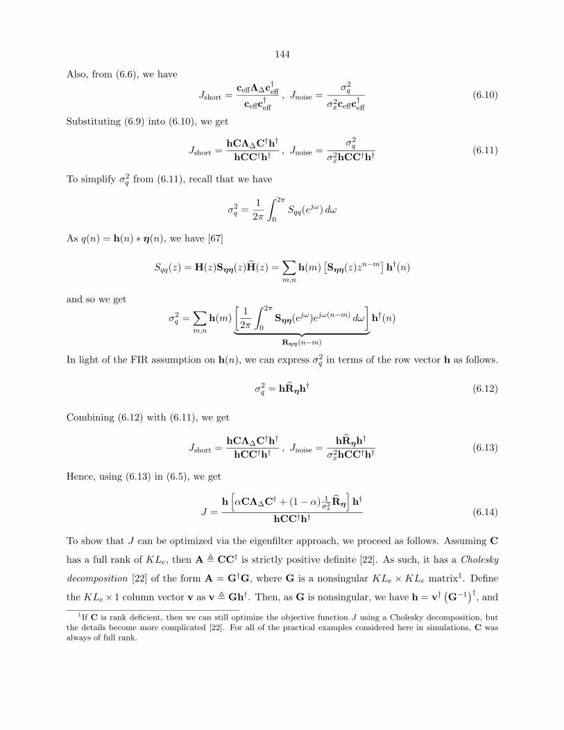
144

Also, from (6.6), we have

Jshort =ceffΛ∆c†effceffc

†eff

, Jnoise =σ2

q

σ2xceffc

†eff

(6.10)

Substituting (6.9) into (6.10), we get

Jshort =hCΛ∆C†h†

hCC†h† , Jnoise =σ2

q

σ2xhCC†h† (6.11)

To simplify σ2q from (6.11), recall that we have

σ2q =

12π

∫ 2π

0Sqq(ejω) dω

As q(n) = h(n) ∗ η(n), we have [67]

Sqq(z) = H(z)Sηη(z)H(z) =∑m,n

h(m)[Sηη(z)zn−m

]h†(n)

and so we get

σ2q =

∑m,n

h(m)[

12π

∫ 2π

0Sηη(ejω)ejω(n−m) dω

]︸ ︷︷ ︸

Rηη (n−m)

h†(n)

In light of the FIR assumption on h(n), we can express σ2q in terms of the row vector h as follows.

σ2q = hRηh† (6.12)

Combining (6.12) with (6.11), we get

Jshort =hCΛ∆C†h†

hCC†h† , Jnoise =hRηh†

σ2xhCC†h† (6.13)

Hence, using (6.13) in (6.5), we get

J =h[αCΛ∆C† + (1 − α) 1

σ2xRη

]h†

hCC†h† (6.14)

To show that J can be optimized via the eigenfilter approach, we proceed as follows. Assuming C

has a full rank of KLe, then A � CC† is strictly positive definite [22]. As such, it has a Cholesky

decomposition [22] of the form A = G†G, where G is a nonsingular KLe × KLe matrix1. Define

the KLe × 1 column vector v as v � Gh†. Then, as G is nonsingular, we have h = v† (G−1)†, and

1If C is rank deficient, then we can still optimize the objective function J using a Cholesky decomposition, butthe details become more complicated [22]. For all of the practical examples considered here in simulations, C wasalways of full rank.

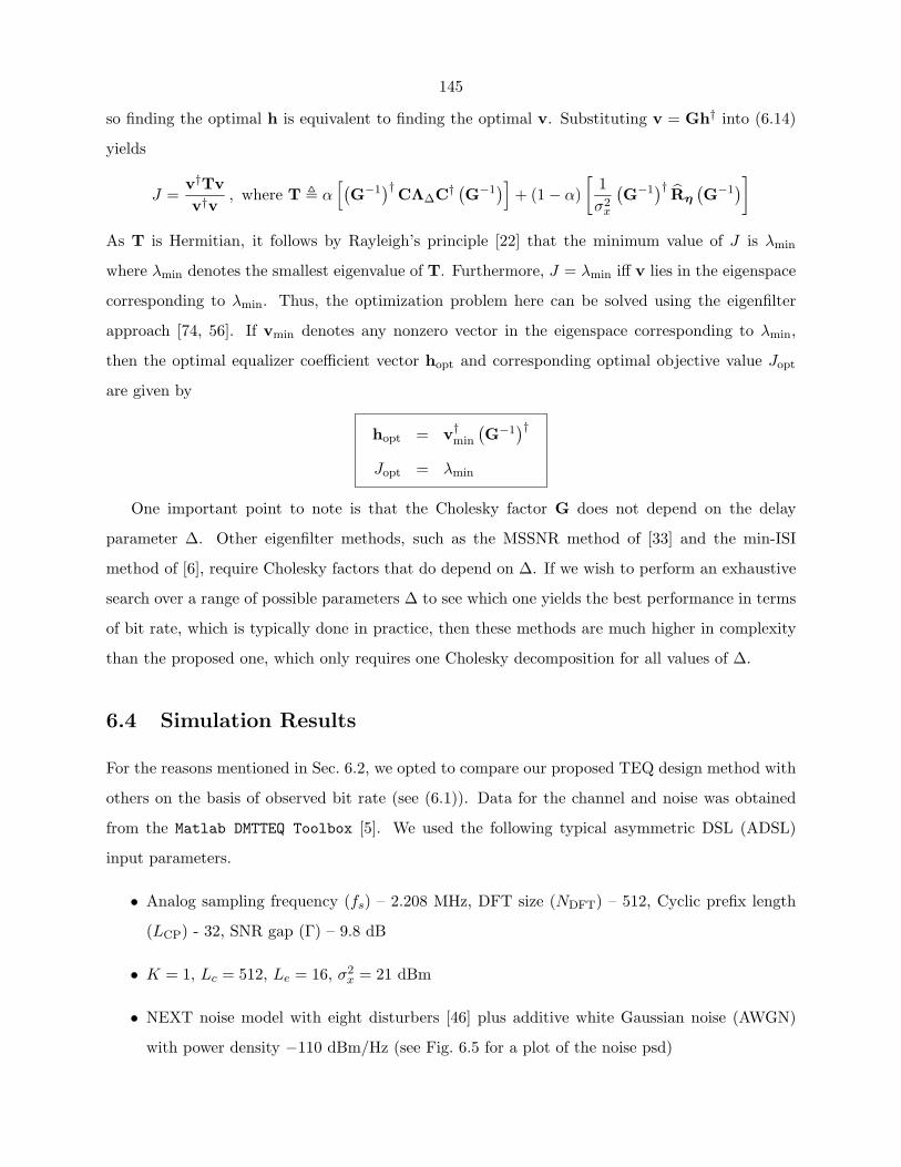
145

so finding the optimal h is equivalent to finding the optimal v. Substituting v = Gh† into (6.14)

yields

J =v†Tvv†v

, where T � α[(

G−1)† CΛ∆C† (G−1

)]+ (1 − α)

[1σ2

x

(G−1

)† Rη

(G−1

)]As T is Hermitian, it follows by Rayleigh’s principle [22] that the minimum value of J is λmin

where λmin denotes the smallest eigenvalue of T. Furthermore, J = λmin iff v lies in the eigenspace

corresponding to λmin. Thus, the optimization problem here can be solved using the eigenfilter

approach [74, 56]. If vmin denotes any nonzero vector in the eigenspace corresponding to λmin,

then the optimal equalizer coefficient vector hopt and corresponding optimal objective value Jopt

are given by

hopt = v†min

(G−1

)†Jopt = λmin

One important point to note is that the Cholesky factor G does not depend on the delay

parameter ∆. Other eigenfilter methods, such as the MSSNR method of [33] and the min-ISI

method of [6], require Cholesky factors that do depend on ∆. If we wish to perform an exhaustive

search over a range of possible parameters ∆ to see which one yields the best performance in terms

of bit rate, which is typically done in practice, then these methods are much higher in complexity

than the proposed one, which only requires one Cholesky decomposition for all values of ∆.

6.4 Simulation Results

For the reasons mentioned in Sec. 6.2, we opted to compare our proposed TEQ design method with

others on the basis of observed bit rate (see (6.1)). Data for the channel and noise was obtained

from the Matlab DMTTEQ Toolbox [5]. We used the following typical asymmetric DSL (ADSL)

input parameters.

• Analog sampling frequency (fs) – 2.208 MHz, DFT size (NDFT) – 512, Cyclic prefix length

(LCP) - 32, SNR gap (Γ) – 9.8 dB

• K = 1, Lc = 512, Le = 16, σ2x = 21 dBm

• NEXT noise model with eight disturbers [46] plus additive white Gaussian noise (AWGN)

with power density −110 dBm/Hz (see Fig. 6.5 for a plot of the noise psd)

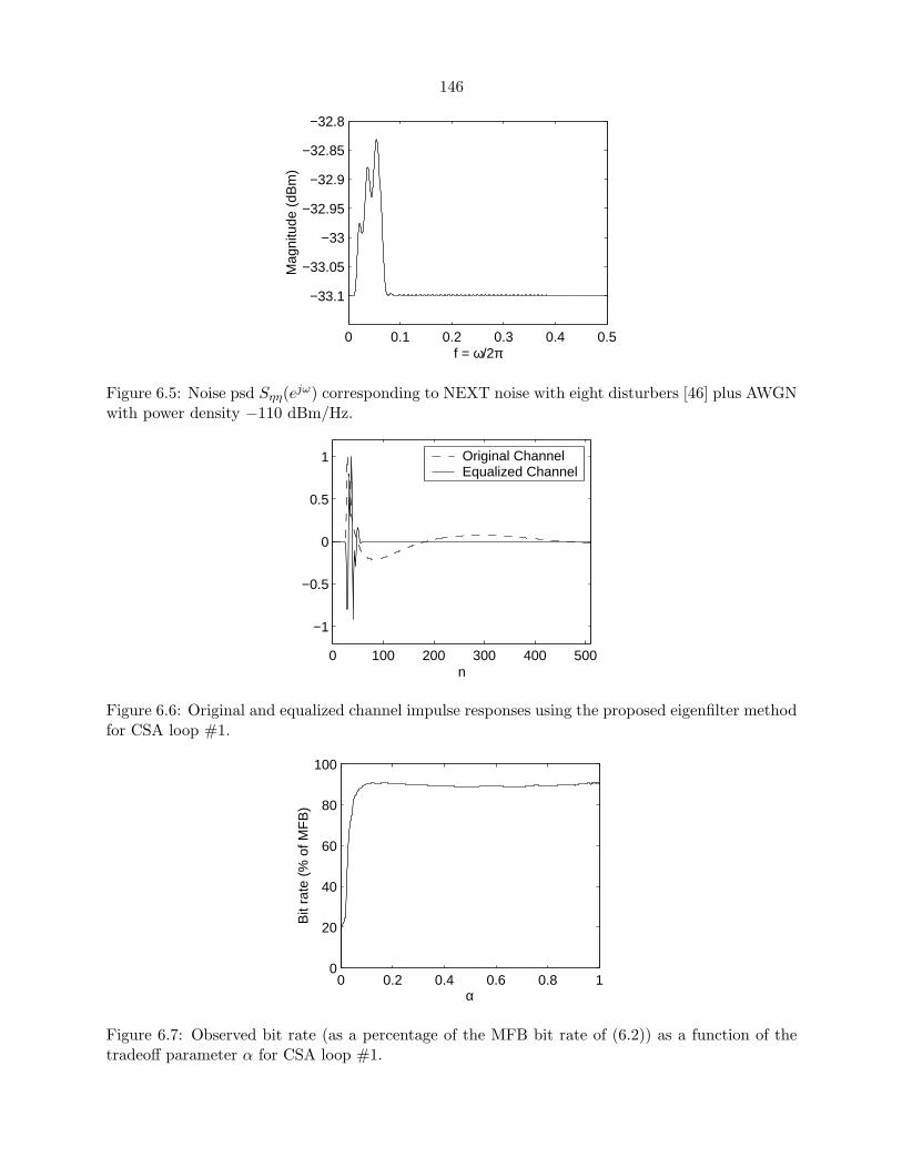
146

0 0.1 0.2 0.3 0.4 0.5

−33.1

−33.05

−33

−32.95

−32.9

−32.85

−32.8

f = ω/2π

Mag

nitu

de (

dBm

)

Figure 6.5: Noise psd Sηη(ejω) corresponding to NEXT noise with eight disturbers [46] plus AWGNwith power density −110 dBm/Hz.

0 100 200 300 400 500

−1

−0.5

0

0.5

1

n

Original ChannelEqualized Channel

Figure 6.6: Original and equalized channel impulse responses using the proposed eigenfilter methodfor CSA loop #1.

0 0.2 0.4 0.6 0.8 10

20

40

60

80

100

α

Bit

rate

(%

of M

FB

)

Figure 6.7: Observed bit rate (as a percentage of the MFB bit rate of (6.2)) as a function of thetradeoff parameter α for CSA loop #1.

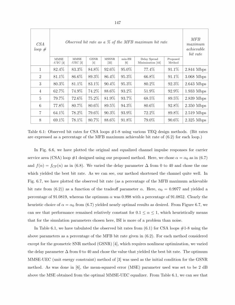
147

CSAloop #

Observed bit rate as a % of the MFB maximum bit rateMFB

maximumachievablebit rate

MMSE-UTC [3]

MMSE-UEC [3]

GSNR[4]

MSSNR[33]

min-ISI[6]

Delay SpreadMinimization [44]

ProposedMethod

1 82.4% 83.3% 84.8% 92.6% 95.0% 77.4% 91.1% 2.844 Mbps

2 81.1% 86.6% 89.3% 86.4% 95.3% 66.8% 91.1% 3.068 Mbps

3 80.3% 81.1% 83.1% 90.4% 95.3% 80.2% 92.3% 2.643 Mbps

4 62.7% 74.9% 74.2% 88.6% 93.2% 51.9% 92.9% 1.933 Mbps

5 79.7% 72.6% 75.2% 81.9% 93.7% 68.5% 89.5% 2.839 Mbps

6 77.8% 80.7% 80.6% 89.5% 94.3% 80.6% 92.8% 2.350 Mbps

7 64.1% 78.2% 79.6% 90.3% 93.9% 72.2% 89.8% 2.519 Mbps

8 69.1% 78.1% 80.7% 88.6% 91.8% 79.0% 90.6% 2.325 Mbps

Table 6.1: Observed bit rates for CSA loops #1-8 using various TEQ design methods. (Bit ratesare expressed as a percentage of the MFB maximum achievable bit rate of (6.2) for each loop.)

In Fig. 6.6, we have plotted the original and equalized channel impulse responses for carrier

service area (CSA) loop #1 designed using our proposed method. Here, we chose α = α0 as in (6.7)

and f(n) = fCP(n) as in (6.8). We varied the delay parameter ∆ from 0 to 40 and chose the one

which yielded the best bit rate. As we can see, our method shortened the channel quite well. In

Fig. 6.7, we have plotted the observed bit rate (as a percentage of the MFB maximum achievable

bit rate from (6.2)) as a function of the tradeoff parameter α. Here, α0 = 0.9977 and yielded a

percentage of 91.0819, whereas the optimum α was 0.998 with a percentage of 91.0852. Clearly the

heuristic choice of α = α0 from (6.7) yielded nearly optimal results as desired. From Figure 6.7, we

can see that performance remained relatively constant for 0.1 ≤ α ≤ 1, which heuristically means

that for the simulation parameters chosen here, ISI is more of a problem than noise.

In Table 6.1, we have tabulated the observed bit rates from (6.1) for CSA loops #1-8 using the

above parameters as a percentage of the MFB bit rate given in (6.2). For each method considered

except for the geometric SNR method (GSNR) [4], which requires nonlinear optimization, we varied

the delay parameter ∆ from 0 to 40 and chose the value that yielded the best bit rate. The optimum

MMSE-UEC (unit energy constraint) method of [3] was used as the initial condition for the GSNR

method. As was done in [6], the mean-squared error (MSE) parameter used was set to be 2 dB

above the MSE obtained from the optimal MMSE-UEC equalizer. From Table 6.1, we can see that

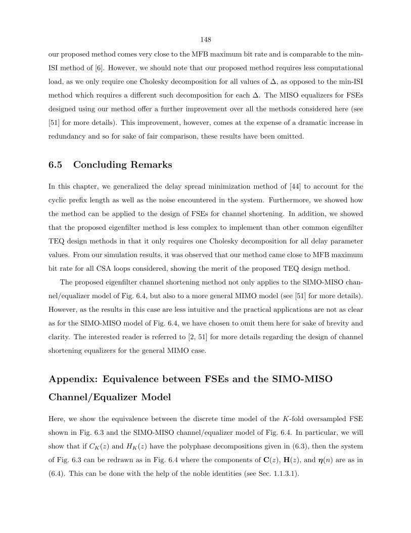
148

our proposed method comes very close to the MFB maximum bit rate and is comparable to the min-

ISI method of [6]. However, we should note that our proposed method requires less computational

load, as we only require one Cholesky decomposition for all values of ∆, as opposed to the min-ISI

method which requires a different such decomposition for each ∆. The MISO equalizers for FSEs

designed using our method offer a further improvement over all the methods considered here (see

[51] for more details). This improvement, however, comes at the expense of a dramatic increase in

redundancy and so for sake of fair comparison, these results have been omitted.

6.5 Concluding Remarks

In this chapter, we generalized the delay spread minimization method of [44] to account for the

cyclic prefix length as well as the noise encountered in the system. Furthermore, we showed how

the method can be applied to the design of FSEs for channel shortening. In addition, we showed

that the proposed eigenfilter method is less complex to implement than other common eigenfilter

TEQ design methods in that it only requires one Cholesky decomposition for all delay parameter

values. From our simulation results, it was observed that our method came close to MFB maximum

bit rate for all CSA loops considered, showing the merit of the proposed TEQ design method.

The proposed eigenfilter channel shortening method not only applies to the SIMO-MISO chan-

nel/equalizer model of Fig. 6.4, but also to a more general MIMO model (see [51] for more details).

However, as the results in this case are less intuitive and the practical applications are not as clear

as for the SIMO-MISO model of Fig. 6.4, we have chosen to omit them here for sake of brevity and

clarity. The interested reader is referred to [2, 51] for more details regarding the design of channel

shortening equalizers for the general MIMO case.

Appendix: Equivalence between FSEs and the SIMO-MISO

Channel/Equalizer Model

Here, we show the equivalence between the discrete time model of the K-fold oversampled FSE

shown in Fig. 6.3 and the SIMO-MISO channel/equalizer model of Fig. 6.4. In particular, we will

show that if CK(z) and HK(z) have the polyphase decompositions given in (6.3), then the system

of Fig. 6.3 can be redrawn as in Fig. 6.4 where the components of C(z), H(z), and η(n) are as in

(6.4). This can be done with the help of the noble identities (see Sec. 1.1.3.1).

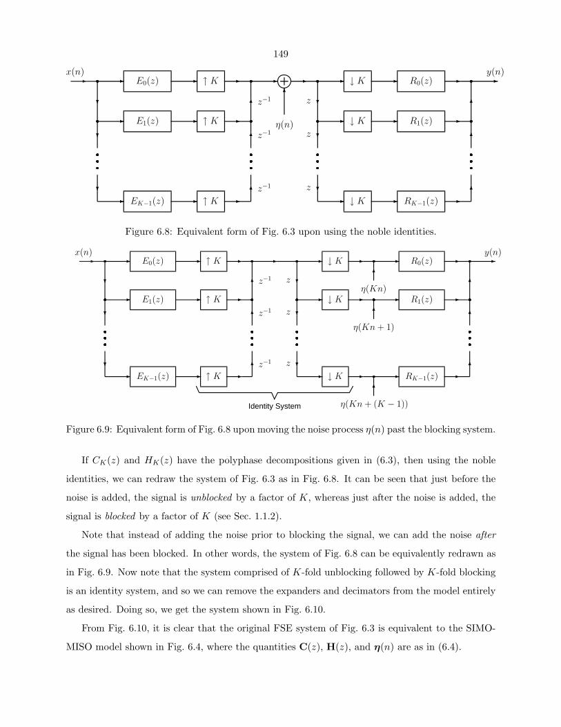
149

� � E0(z)

�

� E1(z)

�

�

� EK−1(z)

�

�

�

↑ K

↑ K

↑ K

z−1

z−1

z−1

�

�

�

�

η(n)

�

�z

�z

�z

x(n)�

�

�

↓ K

↓ K

↓ K

�

�

�

R0(z)

R1(z)

RK−1(z)

�

�

�

�y(n)

Figure 6.8: Equivalent form of Fig. 6.3 upon using the noble identities.

� � E0(z)

�

� E1(z)

�

�

� EK−1(z)

�

�

�

↑ K

↑ K

↑ K

z−1

z−1

z−1

�

�

�

�

�z

�z

�z

x(n)�

�

�

↓ K

↓ K

↓ K

�

�

�

�

�

�

R0(z)

R1(z)

RK−1(z)

�

�

�

�y(n)

η(Kn)

η(Kn + 1)

η(Kn + (K − 1))Identity System

Figure 6.9: Equivalent form of Fig. 6.8 upon moving the noise process η(n) past the blocking system.

If CK(z) and HK(z) have the polyphase decompositions given in (6.3), then using the noble

identities, we can redraw the system of Fig. 6.3 as in Fig. 6.8. It can be seen that just before the

noise is added, the signal is unblocked by a factor of K, whereas just after the noise is added, the

signal is blocked by a factor of K (see Sec. 1.1.2).

Note that instead of adding the noise prior to blocking the signal, we can add the noise after

the signal has been blocked. In other words, the system of Fig. 6.8 can be equivalently redrawn as

in Fig. 6.9. Now note that the system comprised of K-fold unblocking followed by K-fold blocking

is an identity system, and so we can remove the expanders and decimators from the model entirely

as desired. Doing so, we get the system shown in Fig. 6.10.

From Fig. 6.10, it is clear that the original FSE system of Fig. 6.3 is equivalent to the SIMO-

MISO model shown in Fig. 6.4, where the quantities C(z), H(z), and η(n) are as in (6.4).

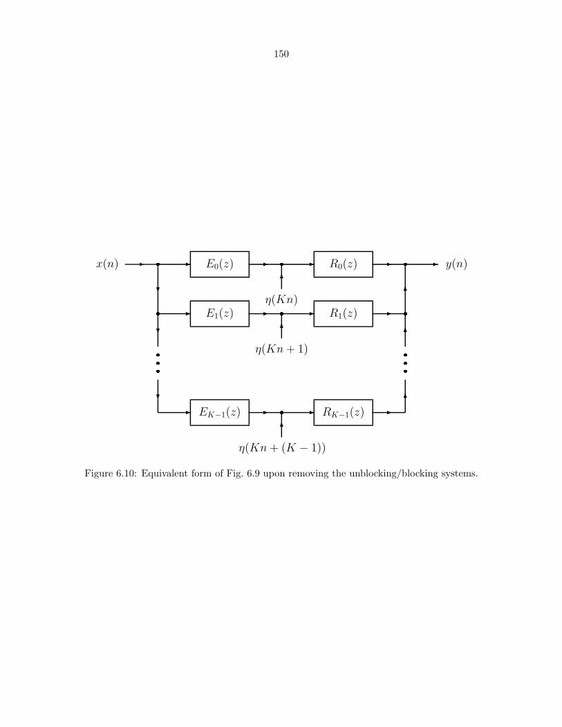
150

� � E0(z)

�

� E1(z)

�

�

� EK−1(z)

x(n) �

�

�

�

�

�

R0(z)

R1(z)

RK−1(z)

�

�

�

� y(n)

η(Kn)

η(Kn + 1)

η(Kn + (K − 1))

Figure 6.10: Equivalent form of Fig. 6.9 upon removing the unblocking/blocking systems.

151

Chapter 7

Conclusion

In this thesis we presented a wide variety of optimization algorithms for the design of realizable

signal-adapted filter banks. Our focus in the first part of the thesis was specifically on the design

of FIR PU signal-adapted filter banks. One of the major contributions was to bridge the gap

between two theoretically optimal PU filter banks, namely, the zeroth-order PCFB (KLT) and the

unconstrained or infinite-order PCFB. This link has previously not been shown in the literature.

As opposed to traditional FIR PU signal-adapted filter bank design methods, in which the filter

bank is chosen to optimize a specific objective for which the PCFB is optimal, the design goals of

the methods presented here were quite different and novel. In particular, in one of the methods

proposed, the design objective was to approximate the infinite-order PCFB itself in the least-

squares sense with a realizable FIR PU filter bank. Using an important complete characterization

of FIR PU systems in terms of degree-one Householder-like building blocks, we showed how to

optimize each parameter seperately, which in turn led to an iterative greedy algorithm for solving

the original least-squares problem. Simulation results for this and other methods presented here

showed that the FIR PU filter banks designed exhibited PCFB-like behavior. The FIR filter banks

designed were shown to monotonically behave more and more like the infinite-order PCFB as the

FIR order increased. This monotonic behavior was shown in terms of numerous objectives for

which the PCFB is optimal. These results served to bridge the gap between the zeroth-order KLT

and infinite-order PCFB which previously had not been reported in the literature.

In the second part of the thesis, we focused on the design of a signal-adapted filter bank in which

the analysis and synthesis filters were FIR but otherwise unconstrained. The model considered was

a uniform filter bank with scalar quantizers in the subbands. Under the high bit rate assumption, we

showed how to obtain either the optimal analysis or synthesis bank using the trick of completing the

square. This in turn led to another iterative greedy algorithm in which the analysis and synthesis

152

banks were alternately optimized. The main contribution of the algorithm here was shown through

simulations presented here. In particular, the FIR filter banks designed exhibited a monotonic

tendency toward information theoretic bounds on distortion and coding gain as the FIR filter

orders increased. Though this result is intuitive, it has not formally been shown in the literature

until now.

In the third part of the thesis, we showed how some of the optimization techniques used for

the design of signal-adapted filter banks could be used for designing channel shortening equalizers.

Here, we showed how the eigenfilter method could be used for the design of good TEQs for DMT

systems. As opposed to other eigenfilter TEQ design methods which require a different Cholesky

factor for every delay parameter considered, the proposed method only required one such factor for

all delays. In addition to being low in computational complexity, the proposed method was shown

to perform nearly optimally in terms of observed bit rate in simulations presented here.

Matlab code for several of the algorithms presented in this thesis will soon be available at [60].

7.1 Open Problems

Despite the contributions related to the design of realizable signal-adapted filter banks presented

here, a number of problems still remain open. First of all, note that all of the algorithms proposed

here apply only to uniform filter banks. In several wavelet-based lossy data compression schemes,

a nonuniform filter bank is commonly used to achieve compression [41, 39]. At this time, it is not

known how to generalize the proposed optimization algorithms to nonuniform filter banks. It should

be noted that any nonuniform filter bank can be equivalently redrawn as a uniform filter bank with

restrictions on the polyphase matrices [67]. Hence, in order to use the algorithms proposed here,

we would have to account for these restrictions along with inherent FIR assumption and any other

constraints such as the PU condition.

Another problem that also remains open is generalizing the FIR PU design algorithms to the

multidimensional case. This may be useful, for example, in image or video processing if we seek an

optimal nonseparable filter bank for compression. The problem in the general multidimensional case

is that there is no known complete parameterization of FIR PU systems in terms of Householder-like

degree-one building blocks as in the one-dimensional case. Though FIR PU factorizations similar

to those given in Sec. 3.2 exist for the multidimensional case, they do not cover all such systems

and are as such incomplete.

153

On a practical note, one issue which remains unresolved is how the iterative greedy algorithms

will perform when the input signal statistics rapidly fluctuate and must be adaptively updated.

This phenomenon commonly occurs in audio signal processing where the assumed stationarity is

only valid for short periods of time.

Another issue which remains unanswered at this point in time is whether the algorithms pro-

posed here can be used in applications outside of source coding and data compresson. In particular,

it is not known if the design methods proposed here can be used for channel coding applications

in digital communications. Typically, in digital communications, a redundant transmultiplexer is

used and the design objectives are quite different in nature than those considered for data compres-

sion. Nevertheless, it would be interesting to see whether the proposed design algorithms could be

used for this application. For the FIR PU design algorithms proposed here, this widely depends on

whether the theory of PCFBs can be applied to redundant transmultiplexers. The theory of PCFBs,

which has been found useful for nonredundant transmultiplexers, has not yet been extended for the

redundant case.

154

Bibliography

[1] S. Akkarakaran and P. P. Vaidyanathan, “Filterbank optimization with convex objectives and

the optimality of principal component forms,” IEEE Trans. Signal Processing, vol. 49, no. 1,

pp. 100–114, Jan. 2001.

[2] N. Al-Dhahir, “FIR channel-shortening equalizers for MIMO ISI channels,” IEEE Trans. Com-

mun., vol. 49, no. 2, pp. 213–218, Feb. 2001.

[3] N. Al-Dhahir and J. M. Cioffi, “Efficiently computed reduced-parameter input-aided MMSE

equalizers for ML detection: a unified approach,” IEEE Trans. Inform. Theory, vol. 42, no. 3,

pp. 903–915, May 1996.

[4] ——, “A bandwidth-optimized reduced-complexity equalized multicarrier transceiver,” IEEE

Trans. Commun., vol. 45, no. 8, pp. 948–956, Aug. 1997.

[5] G. Arslan, M. Ding, B. Lu, M. Milosevic, Z. Shen, and B. L. Evans. (2003)

Matlab DMTTEQ Toolbox. [Online]. Available: http://www.ece.utexas.edu/ be-

vans/projects/adsl/dmtteq/dmtteq.html

[6] G. Arslan, B. L. Evans, and S. Kiaei, “Equalization for discrete multitone transceivers to

maximize bit rate,” IEEE Trans. Signal Processing, vol. 49, no. 12, pp. 3123–3135, Dec. 2001.

[7] R. E. Blahut, Principles and Practice of Information Theory. Reading, MA: Addison-Wesley,

1987.

[8] H. Caglar, Y. Liu, and A. N. Akansu, “Statistically optimized PR-QMF design,” in Proc. SPIE

1605, Wavelet Appl. Signal Image Process., San Diego, CA, 1991, pp. 86–94.

[9] P. R. Chevillat and G. Ungerboeck, “Optimum FIR transmitter and receiver filters for data

transmission over band-limited channels,” IEEE Trans. Commun., vol. COM-30, no. 8, pp.

1909–1915, Aug. 1982.

155

[10] T. M. Cover and J. A. Thomas, Elements of Information Theory. New York, NY: John Wiley

& Sons, 1991.

[11] P. Delsarte, B. Macq, and D. T. M. Slock, “Signal-adapted multiresolution transform for image

coding,” IEEE Trans. Inform. Theory, vol. 38, no. 2, pp. 897–904, Mar. 1992.

[12] I. Djokovic and P. P. Vaidyanathan, “Results on biorthogonal filter banks,” Journal of Applied

and Computational Harmonic Analysis, vol. 1, pp. 329–343, 1994.

[13] N. J. Fliege, Multirate Digital Signal Processing: Multirate Systems - Filter Banks - Wavelets.

Chichester, England: John Wiley & Sons, 1994.

[14] G. B. Giannakis, “Filterbanks for blind channel identification and equalization,” IEEE Signal

Processing Lett., vol. 4, no. 6, pp. 184–187, June 1997.

[15] G. B. Giannakis, Y. Hua, P. Stoica, and L. Tong, Signal Processing Advances in Wireless and

Mobile Communications, Volume 1: Trends in Channel Estimation and Equalization. Upper

Saddle River, NJ: Prentice-Hall, 2000.

[16] ——, Signal Processing Advances in Wireless and Mobile Communications, Volume 2: Trends

in Single- and Multi-User Systems. Upper Saddle River, NJ: Prentice-Hall, 2000.

[17] G. B. Giannakis, Z. Wang, A. Scaglione, and S. Barbarossa, “AMOUR-generalized multicarrier

CDMA irrespective of multipath,” in Proc. Global Telecommunications Conference, vol. 1B,

Rio de Janeireo, Brazil, Dec. 1999, pp. 965–969.

[18] ——, “AMOUR-generalized multicarrier transceivers for blind CDMA regardless of multi-

path,” IEEE Trans. Commun., vol. 48, no. 12, pp. 2064–2076, Dec. 2000.

[19] A. Hjørungnes, H. Coward, and T. A. Ramstad, “Minimum mean square error FIR filter banks

with arbitrary filter lengths,” in Proc. Int. on Image Processing, vol. 1, Kobe, Japan, Oct. 1999,

pp. 619–623.

[20] A. Hjørungnes and T. A. Ramstad, “Algorithm for jointly optimized analysis and synthesis

FIR filter banks,” in Proc. IEEE Int. Conf. on Electron., Circuits, and Systems, vol. 1, Pafos,

Cyprus, Sept. 1999, pp. 369–372.

156

[21] A. Hjørungnes and T. Saramaki, “Minimum mean square error nonuniform FIR filter banks,”

in Proc. IEEE Int. Conf. on Acoust., Speech, and Signal Processing, vol. 6, Salt Lake City,

UT, May 2001, pp. 3609–3612.

[22] R. A. Horn and C. R. Johnson, Matrix Analysis. Cambridge, U.K.: Cambridge University

Press, 1985.

[23] Y. Huang and P. M. Schultheiss, “Block quantization of correlated Gaussian random variables,”

IEEE Trans. Commun. Syst., vol. C-10, pp. 289–296, Sept. 1963.

[24] O. S. Jahromi, B. A. Francis, and R. H. Kwong, “Algebraic theory of optimal filterbanks,”

IEEE Trans. Signal Processing, vol. 51, no. 2, pp. 442–457, Feb. 2003.

[25] N. S. Jayant and P. Noll, Digital Coding of Waveforms: Principles and Applications to Speech

and Video. Englewood Cliffs, NJ: Prentice-Hall, 1984.

[26] I. Kalet, “The multitone channel,”IEEE Trans. Commun., vol.37, no.2, pp. 119–124, Feb.1989.

[27] A. Kırac and P. P. Vaidyanathan, “On existence of FIR principal component filter banks,” in

Proc. IEEE Int. Conf. on Acoust., Speech, and Signal Processing, vol. 3, Seattle, WA, May

1998, pp. 1329–1332.

[28] ——, “Optimality of orthonormal transforms for subband coding,” in Proc. IEEE DSP Work-

shop, Bryce Canyon, UT, Aug. 1998.

[29] ——, “Theory and design of optimum FIR compaction filters,” IEEE Trans. Signal Processing,

vol. 46, no. 4, pp. 903–919, Apr. 1998.

[30] J. Kovacevic and M. Vetterli, “Perfect reconstruction filter banks with rational sampling fac-

tors,” IEEE Trans. Signal Processing, vol. 41, no. 6, pp. 2047–2066, June 1993.

[31] B. Maison and L. Vandendorpe, “About the asymptotic performance of multiple-

input/multiple-output linear prediction of subband signals,” IEEE Signal Processing Lett.,

vol. 5, no. 12, pp. 315–317, Dec. 1998.

[32] S. Mallat, AWavelet Tour of Signal Processing, 2nd ed. San Diego, CA: Academic Press, 1999.

[33] P. J. W. Melsa, R. C. Younce, and C. E. Rohrs, “Impulse response shortening for discrete

multitone transceivers,” IEEE Trans. Commun., vol. 44, no. 12, pp. 1662–1672, Dec. 1996.

157

[34] T. K. Moon and W. C. Stirling, Mathematical Methods and Algorithms for Signal Processing.

Upper Saddle River, NJ: Prentice-Hall, 2000.

[35] P. Moulin, M. Anitescu, K. O. Kortanek, and F. A. Potra, “The role of linear semi-infinite

programming in signal-adapted QMF bank design,” IEEE Trans. Signal Processing, vol. 45,

no. 9, pp. 2160–2174, Sept. 1997.

[36] P. Moulin, M. Anitescu, and K. Ramchandran, “Theory of rate-distortion-optimal, constrained

filterbanks–application to IIR and FIR biorthogonal designs,” IEEE Trans. Signal Processing,

vol. 48, no. 4, pp. 1120–1132, Apr. 2000.

[37] P. Moulin and M. K. Mıhcak, “Theory and design of signal-adapted FIR paraunitary filter

banks,” IEEE Trans. Signal Processing, vol. 46, no. 4, pp. 920–929, Apr. 1998.

[38] J. G. Proakis, Digital Communications, 4th ed. New York, NY: McGraw-Hill, 2000.

[39] D. Salomon, A Guide to Data Compression Methods. New York, NY: Springer-Verlag, 2002.

[40] V. P. Sathe and P. P. Vaidyanathan, “Effects of multirate systems on the statistical properties

of random signals,” IEEE Trans. Signal Processing, vol. 41, no. 1, pp. 131–146, Jan. 1993.

[41] K. Sayood, Introduction to Data Compression, 2nd ed. San Diego, CA: Academic Press, 2000.

[42] A. Scaglione, G. B. Giannakis, and S. Barbarossa, “Redundant filterbank precoders and equal-

izers: Part I: unification and optimal designs,” IEEE Trans. Signal Processing, vol. 47, no. 7,

pp. 1988–2006, July 1999.

[43] ——, “Redundant filterbank precoders and equalizers: Part II: blind channel estimation, syn-

chronization, and direct equalization,” IEEE Trans. Signal Processing, vol. 47, no. 7, pp.

2007–2022, July 1999.

[44] R. Schur and J. Speidel, “An efficient equalization method to minimize delay spread in

OFDM/DMT systems,” in Proc. IEEE Int. Conf. on Communications, vol. 5, Helsinki, Fin-

land, June 2001, pp. 1481–1485.

[45] A. K. Soman and P. P. Vaidyanathan, “On orthonormal wavelets and paraunitary filter banks,”

IEEE Trans. Signal Processing, vol. 41, no. 3, pp. 1170–1183, Mar. 1993.

158

[46] T. Starr, J. M. Cioffi, and P. J. Silverman, Understanding Digital Subscriber Line Technology.

Upper Saddle River, NJ: Prentice-Hall, 1999.

[47] G. Strang and T. Nguyen, Wavelets and Filter Banks. Wellesley, MA: Wellesley-Cambridge

Press, 1996.

[48] C. W. Therrien, Discrete Random Signals and Statistical Signal Processing. Upper Saddle

River, NJ: Prentice-Hall, 1992.

[49] A. Tkacenko and P. P. Vaidyanathan, “Iterative gradient based greedy algorithm for the design

of optimal FIR compaction filters and signal-adapted paraunitary filter banks,” submitted to

IEEE Trans. Signal Processing.

[50] ——, “Iterative greedy algorithm for solving the FIR paraunitary approximation problem,”

submitted to IEEE Trans. Signal Processing.

[51] ——, “Eigenfilter design of MIMO equalizers for channel shortening,” in Proc. IEEE Int. Conf.

on Acoust., Speech, and Signal Processing, vol. 3, Orlando, FL, May 2002, pp. 2361–2364.

[52] ——, “A new eigenfilter based method for optimal design of channel shortening equalizers,”

in Proc. IEEE Int. Symp. on Circuits and Systems, vol. 2, Scottsdale, AZ, May 2002, pp.

504–507.

[53] ——, “Noise optimized eigenfilter design of time-domain equalizers for DMT systems,” in Proc.

IEEE Int. Conf. on Communications, vol. 1, New York, NY, Apr./May 2002, pp. 54–58.

[54] ——, “Iterative eigenfilter method for designing optimum overdecimated orthonormal FIR

compaction filter banks,” in Proc. 37th Asilomar Conference on Signals, Systems and Com-

puters, Pacific Grove, CA, Nov. 2003.

[55] ——, “A low-complexity eigenfilter design method for channel shortening equalizers for DMT

systems,” IEEE Trans. Commun., vol. 51, no. 7, pp. 1069–1072, July 2003.

[56] ——, “On the eigenfilter design method and its applications: a tutorial,” IEEE Trans. Circuits

Syst. II, vol. 50, no. 9, pp. 497–517, Sept. 2003.

[57] ——, “On the least squares signal approximation model for overdecimated rational nonuni-

form filter banks and applications,” in Proc. IEEE Int. Conf. on Acoust., Speech, and Signal

Processing, vol. 6, Hong Kong, China, Apr. 2003, pp. 481–484.

159

[58] ——, “Iterative algorithm for the design of optimal FIR analysis/synthesis filters for overdec-

imated filter banks,” accepted to IEEE Int. Symp. on Circuits and Systems, May 2004.

[59] ——, “Iterative gradient technique for the design of least squares optimal FIR magnitude

squared nyquist filters,” accepted to IEEE Int. Conf. on Acoust., Speech, and Signal Processing,

May 2004.

[60] A. Tkacenko. (2004) Matlab Signal-Adapted Filter Bank Optimization Algorithms. [Online].

Available: http://www.systems.caltech.edu/dsp/students/andre/index.html

[61] J. R. Treichler, I. Fijalkow, and J. C. R. Johnson, “Fractionally spaced equalizers: How long

should they really be?” IEEE Signal Processing Mag., vol. 13, no. 3, pp. 65–81, May 1996.

[62] M. K. Tsatsanis and G. B. Giannakis, “Principal component filter banks for optimal multires-

olution analysis,” IEEE Trans. Signal Processing, vol. 43, no. 8, pp. 1766–1777, Aug. 1995.

[63] D. W. Tufts and J. T. Francis, “Designing digital lowpass filters: comparison of some methods

and criteria,” IEEE Trans. Audio Electroacoust., vol. AU-18, pp. 487–494, Dec. 1970.

[64] J. Tuqan and P. P. Vaidyanathan, “A state space approach to the design of globally optimal

FIR energy compaction filters,” IEEE Trans. Signal Processing, vol. 48, no. 10, pp. 2822–2838,

Oct. 2000.

[65] M. Unser, “An extension of the KLT for wavelets and perfect reconstruction filter banks,” in

Proc. SPIE 2034, Wavelet Appl. Signal Image Process., San Diego, CA, 1993, pp. 45–56.

[66] ——, “On the optimality of ideal filters for pyramid and wavelet signal approximation,” IEEE

Trans. Signal Processing, vol. 41, no. 12, pp. 3591–3596, Dec. 1993.

[67] P. P. Vaidyanathan, Multirate Systems and Filter Banks. Englewood Cliffs, NJ: Prentice-Hall,

1993.

[68] ——, “Theory of optimal orthonormal subband coders,” IEEE Trans. Signal Processing,

vol. 46, no. 6, pp. 1528–1543, June 1998.

[69] P. P. Vaidyanathan and S. Akkarakaran, “A review of the theory and applications of optimal

subband and transform coders,” Journal of Applied and Computational Harmonic Analysis,

vol. 10, pp. 254–289, 2001.

160

[70] P. P. Vaidyanathan and P. Q. Hoang, “Lattice structures for optimal design and robust imple-

mentation of two-channel perfect-reconstruction QMF banks,” IEEE Trans. Acoust., Speech,

Signal Processing, vol. 36, no. 1, pp. 81–94, Jan. 1988.

[71] P. P. Vaidyanathan and A. Kırac, “Cyclic LTI systems and the paraunitary interpolation

problem,” in Proc. IEEE Int. Conf. on Acoust., Speech, and Signal Processing, vol. 3, Seattle,

WA, May 1998, pp. 1445–1448.

[72] ——, “Results on optimal biorthogonal filter banks,” IEEE Trans. Circuits Syst. II, vol. 45,

no. 8, pp. 932–947, Aug. 1998.

[73] P. P. Vaidyanathan, Y.-P. Lin, S. Akkarakaran, and S.-M. Phoong, “Discrete multitone mod-

ulation with principal component filter banks,” IEEE Trans. Circuits Syst. I, vol. 49, no. 10,

pp. 1397–1412, Oct. 2002.

[74] P. P. Vaidyanathan and T. Q. Nguyen, “Eigenfilters: a new approach to least-squares FIR filter

design and applications including Nyquist filters,” IEEE Trans. Circuits Syst., vol. CAS-34,

no. 1, pp. 11–23, Jan. 1987.

[75] P. P. Vaidyanathan, T. Q. Nguyen, Z. Doganata, and T. Saramaki, “Improved technique for

design of perfect reconstruction FIR QMF banks with lossless polyphase matrices,” IEEE

Trans. Acoust., Speech, Signal Processing, vol. 37, no. 7, pp. 1042–1056, July 1989.

[76] P. P. Vaidyanathan and B. Vrcelj, “Biorthogonal partners and applications,” IEEE Trans.

Signal Processing, vol. 49, no. 5, pp. 1013–1027, May 2001.

[77] B. Vrcelj and P. P. Vaidyanathan, “Least squares signal approximation using multirate systems:

multichannel nonuniform case,” in Proc. 35th Asilomar Conference on Signals, Systems and

Computers, vol. 1, Pacific Grove, CA, Nov. 2001, pp. 553–557.

[78] ——, “MIMO biorthogonal partners and applications,” IEEE Trans. Signal Processing, vol. 50,

no. 3, pp. 528–542, Mar. 2002.

[79] B. Xuan and R. H. Bamberger, “FIR principal component filter banks,” IEEE Trans. Signal

Processing, vol. 46, no. 4, pp. 930–940, Apr. 1998.