optimization and openmp parallelization of …€¦ · optimization and openmp parallelization of a...

OPTIMIZATION AND OPENMP PARALLELIZATION

OF A DISCRETE ELEMENT CODE FOR CONVEX

POLYHEDRA ON MULTI-CORE MACHINES

JIAN CHEN

Advanced Institute for Computational Science (AICS)RIKEN, 7-1-26, Minatojima-minami-machi

Chuo-Ku, Kobe, Hyogo 650-0047, Japan

[email protected]

HANS-GEORG MATUTTIS

Department of Mechanical Engineering and Intelligent Systems

The University of Electro-Communications1-5-1 Chofugaoka, Chofu, Tokyo 182-8585, Japan

[email protected]

Received 23 October 2012

Accepted 29 October 2012

Published 14 December 2012

We report our experiences with the optimization and parallelization of a discrete element code

for convex polyhedra on multi-core machines and introduce a novel variant of the sort-and-

sweep neighborhood algorithm. While in theory the whole code in itself parallelizes ideally, in

practice the results on di®erent architectures with di®erent compilers and performance mea-surement tools depend very much on the particle number and optimization of the code. After

di±culties with the interpretation of the data for speedup and e±ciency are overcome, re-

spectable parallelization speedups could be obtained.

Keywords: OpenMP; DEM; polyhedra; INTEL; AMD.

PACS Nos.: 11.25.Hf, 123.1K.

1. Introduction

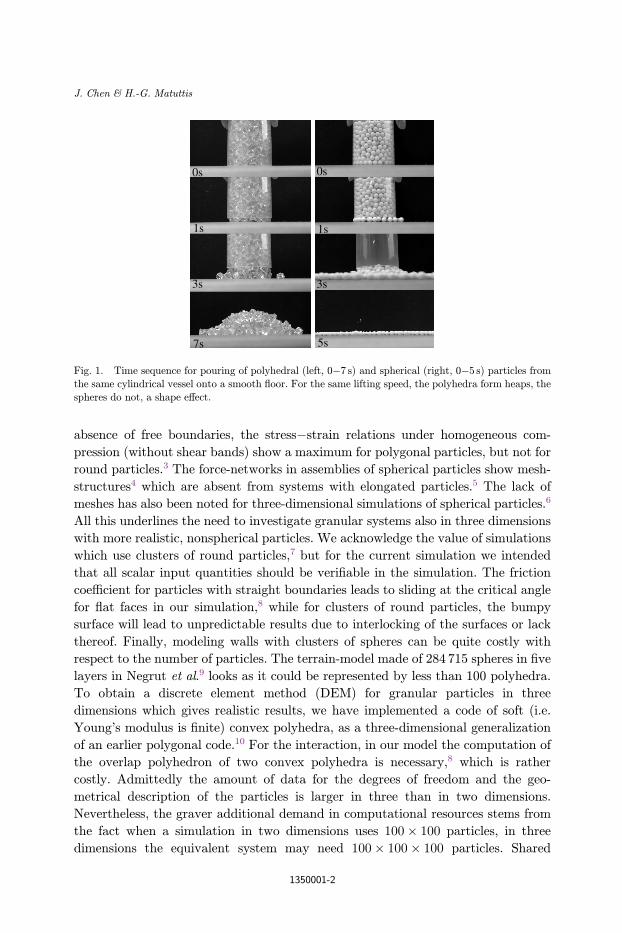
For granular materials near surfaces, shape e®ects are quite obvious: On °at surfaces,

polyhedral particles form heaps easily, while round particles roll away and no heap

can be built, as in Fig. 1. The system size or particle number does not help matters:

though the round particles are smaller and the particle number is higher, heap

formation fails to manifest. Also other properties are largely di®erent between sys-

tems with spherical and nonspherical particles. Apart from the angle of repose and

coordination number, heaps of nonspherical particles show history e®ects.1,2 In the

International Journal of Modern Physics C

Vol. 24, No. 2 (2013) 1350001 (24 pages)

#.c World Scienti¯c Publishing CompanyDOI: 10.1142/S0129183113500010

1350001-1

http://dx.doi.org/10.1142/S0129183113500010

absence of free boundaries, the stress�strain relations under homogeneous com-

pression (without shear bands) show a maximum for polygonal particles, but not for

round particles.3 The force-networks in assemblies of spherical particles show mesh-

structures4 which are absent from systems with elongated particles.5 The lack of

meshes has also been noted for three-dimensional simulations of spherical particles.6

All this underlines the need to investigate granular systems also in three dimensions

with more realistic, nonspherical particles. We acknowledge the value of simulations

which use clusters of round particles,7 but for the current simulation we intended

that all scalar input quantities should be veri¯able in the simulation. The friction

coe±cient for particles with straight boundaries leads to sliding at the critical angle

for °at faces in our simulation,8 while for clusters of round particles, the bumpy

surface will lead to unpredictable results due to interlocking of the surfaces or lack

thereof. Finally, modeling walls with clusters of spheres can be quite costly with

respect to the number of particles. The terrain-model made of 284 715 spheres in ¯ve

layers in Negrut et al.9 looks as it could be represented by less than 100 polyhedra.

To obtain a discrete element method (DEM) for granular particles in three

dimensions which gives realistic results, we have implemented a code of soft (i.e.

Young's modulus is ¯nite) convex polyhedra, as a three-dimensional generalization

of an earlier polygonal code.10 For the interaction, in our model the computation of

the overlap polyhedron of two convex polyhedra is necessary,8 which is rather

costly. Admittedly the amount of data for the degrees of freedom and the geo-

metrical description of the particles is larger in three than in two dimensions.

Nevertheless, the graver additional demand in computational resources stems from

the fact when a simulation in two dimensions uses 100� 100 particles, in three

dimensions the equivalent system may need 100� 100� 100 particles. Shared

1s

7s 5s

3s

0s

3s

0s

1s

Fig. 1. Time sequence for pouring of polyhedral (left, 0�7 s) and spherical (right, 0�5 s) particles from

the same cylindrical vessel onto a smooth °oor. For the same lifting speed, the polyhedra form heaps, the

spheres do not, a shape e®ect.

J. Chen & H.-G. Matuttis

1350001-2

memory parallelization via OpenMP o®ers itself as appropriate remedy for the

computational needs, as high parallel e±ciencies can be expected for DEM, as there

are practically no dependencies. We refrained from message-passing parallelization,

as the e®ort required in our experience is equal to that for writing the original code.

Speeding up the simulation with general purpose graphic processing units

(GPGPUs) did not look promising after some initial attempts: GPGPUs are to all

intents and purposes single instruction multiple data (SIMD) processors which are

ill-suited to our overlap computation which is littered with conditional executions.

Depending on the di®erent relative position of the polyhedra and their features

(faces, edges and vertices) the program °ow will change considerably, which is

extremely ill-suited for SIMD-architectures. A short overview over other polyhedral

codes and their performance is given in Sec. 4.2.

2. Program Characteristics

In the following, we give a rough overview over the simulation code8 whose details

have been published elsewhere.2,11 The whole production code is written in FOR-

TRAN90, to avoid the pointer-aliasing problem of C and its derivatives:12 In prin-

ciple, standard-C does not forbid that pointers in the calls of C-functions may point

to overlapping memory locations. The resulting ambiguity of the assignment of the

values to the actual memory location at runtime can make the use of the cache

impossible, so that all data have to be fetched from and written to the main memory,

at tremendous performance losses. In FORTRAN, calling a subroutine with the same

multiple argument is forbidden, and call subroutine(a,a) in any FORTRAN

source code should trigger an error message from the compiler. Therefore, compila-

tion under FORTRAN can optimize the memory access under the assumption that

all memory addresses in a subroutine are unique and make use of the full cache

hierarchy without restrictions. This means that even if FORTRAN-code is converted

into C, as is the case with the GFORTRAN-suite, the backend-C-compiler can

perform more e±cient optimizations than for a C-code with inscrutable pointer

usage.

For the time integration of the equations of motion, we use backward-di®erence-

formulae13 of orders 5 (\6-value Gear predictor and corrector.")14,15 The angular

degrees of freedom and the Euler equations of motion are implemented via unit

quaternions and their time derivatives,15 to avoid the usual singularities for the

equations of motion for the Euler angles.

2.1. Boundary conditions

While up to now we have simulated mainly heap geometries on °at surfaces,2,11 for

parallelization timings a rotating drum ¯lled with particles is more appropriate, so

that the number of particles and therefore the computational e®ort per time-step is

approximately constant throughout the simulation. The particles are dropped from

Optimization and Parallelization of a Discrete Element Code for Convex Polyhedra

1350001-3

their initial positions without any overlap with neighboring particles, and then form

a bed on the °oor of the drum. The rotation of the drum takes care for perpetually

changing neighborhoods, which, together with the realistically evolving packing, is

representative for a dynamic granular system at relative high packing densities. To

evaluate the performance, a time-step size of 2 � 10�5 s was used for two real-second

simulations. For such a simulation setting, the equilibrium (i.e. for performance

evaluation, the long-term average of number of neighbors) is reached within about

10 000 time-steps, so for the remaining 90% of the time-steps, the system is dense and

evolves dynamics. For nonelongated particles in our three-dimensional simulation

the coordination number is about 5. In two dimensions, the coordination number will

be lower, which should not be forgotten when updates per second are compared with

simulations for two dimensions. The drum with inner diameter 140mm and the outer

diameter 200mm, is made from 34 wall particles and rotates with �=6 rad/s. Two

quadratic plates form the lids, 32 trapezoidal prisms with eight vertices and 12 faces

form the drum walls, see Fig. 2. 648 granular particles (polyhedra with 12 vertices

and 20 faces) were initialized with their vertices on the surface of an ellipsoid with

half-axes a; b and c as 8, 8 and 7.5mm, respectively. We add a small randomization

of about 1% in the angles which are used to tessellate the ellipsoid to avoid that the

edges of two contacting polyhedra can coincide. This would lead to degeneracies in

the overlap computation which would be very costly to deal with.

2.2. Neighborhood algorithm

In computational design, robotics and solid modeling, where the \particles" are not

necessarily convex, there is a vast literature on the problem of \neighborhood

algorithms" and \collision detection" (see Ref. 16 and references therein). Usually, it

is convenient to employ a hierarchy of di®erent algorithms, where the fastest ones

give the least precise information and the computationally most expensive ones give

Fig. 2. Drum made from polyhedral wall particles with back plate, front plate not shown.


1350001-4

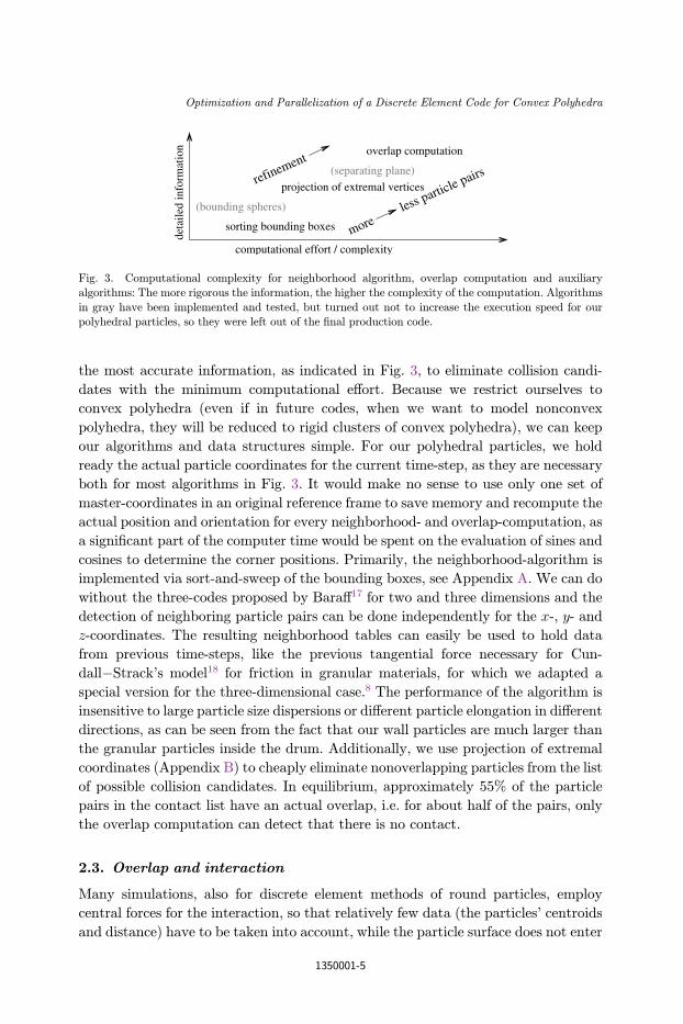
the most accurate information, as indicated in Fig. 3, to eliminate collision candi-

dates with the minimum computational e®ort. Because we restrict ourselves to

convex polyhedra (even if in future codes, when we want to model nonconvex

polyhedra, they will be reduced to rigid clusters of convex polyhedra), we can keep

our algorithms and data structures simple. For our polyhedral particles, we hold

ready the actual particle coordinates for the current time-step, as they are necessary

both for most algorithms in Fig. 3. It would make no sense to use only one set of

master-coordinates in an original reference frame to save memory and recompute the

actual position and orientation for every neighborhood- and overlap-computation, as

a signi¯cant part of the computer time would be spent on the evaluation of sines and

cosines to determine the corner positions. Primarily, the neighborhood-algorithm is

implemented via sort-and-sweep of the bounding boxes, see Appendix A. We can do

without the three-codes proposed by Bara®17 for two and three dimensions and the

detection of neighboring particle pairs can be done independently for the x-, y- and

z-coordinates. The resulting neighborhood tables can easily be used to hold data

from previous time-steps, like the previous tangential force necessary for Cun-

dall�Strack's model18 for friction in granular materials, for which we adapted a

special version for the three-dimensional case.8 The performance of the algorithm is

insensitive to large particle size dispersions or di®erent particle elongation in di®erent

directions, as can be seen from the fact that our wall particles are much larger than

the granular particles inside the drum. Additionally, we use projection of extremal

coordinates (Appendix B) to cheaply eliminate nonoverlapping particles from the list

of possible collision candidates. In equilibrium, approximately 55% of the particle

pairs in the contact list have an actual overlap, i.e. for about half of the pairs, only

the overlap computation can detect that there is no contact.

2.3. Overlap and interaction

Many simulations, also for discrete element methods of round particles, employ

central forces for the interaction, so that relatively few data (the particles' centroids

and distance) have to be taken into account, while the particle surface does not enter

deta

iled

info

rmat

ion

more le

ss particle pairs refinement

computational effort / complexity

(bounding spheres)

sorting bounding boxes

projection of extremal vertices

(separating plane)

overlap computation

Fig. 3. Computational complexity for neighborhood algorithm, overlap computation and auxiliary

algorithms: The more rigorous the information, the higher the complexity of the computation. Algorithms

in gray have been implemented and tested, but turned out not to increase the execution speed for ourpolyhedral particles, so they were left out of the ¯nal production code.


1350001-5

the calculation at all. In that case, computing power is a more serious problem than

memory. In contrast, our algorithm needs a relatively large amount of input data.

Additional to the mere positions, there are connectivity tables, i.e. corner-face table,

which contains the information about the faces intersecting at a speci¯c corner, and

corner-face table, with the information of corners forming a particular face. Together

with the relatively complex overlap computation, this leads to a considerably higher

demand on the memory bandwidth than for round particles, and the program exe-

cution will be delayed more by cache-misses than by the pure computational e®ort.

For the interaction, the overlap polyhedron, its centroid and the contact-line (the

intersection of the two overlapping polyhedral surfaces) have to be computed, the

computation of the forces, torques and their direction is then relatively inexpensive.

To obtain the overlap polyhedron, the penetration points of the edges through

neighboring triangular faces of the polyhedra are computed in every time-step using

the point-normal form of the the edges and faces. This is followed by clipping,

depending on whether the penetration point is inside or outside the triangle. Finally,

from the corners of the overlap polyhedron we can determine the centroid, the

volume and the contact line, which are used to model the interactive force. Details

can be found in Refs. 2, 8 and 11.

3. First Approach: Parallelization of the Overlap Routine Only

3.1. Compilers and hardware

We used Linux-workstations with AMD-processors and a MacBook Pro (MAC OS

10.7 with an INTEL Core i7 processor). The specs of the machines are listed in

Table 1. Compilation on Linux machines was done with the PGI compiler (version

10.2). On the MAC, GFORTRAN-FSF-4.6 from the GCC4.6-suite was used. For

performance analysis, pro¯ling tools of PGI (PGPROF and PGCOLLECT) were

used for the Linux machines and the \Time Pro¯ler" tool from MAC OS 10.7 was

used for the MacBook Pro. OpenMP was used for parallelization. For OpenMP, the

underlying concept of parallelization is thread-parallelization, i.e. threads (data and

the operations acting on it) are executed synchronously on several cores instead of

sequentially on a single core, as long as there are no data dependencies. Before

Table 1. Speci¯cation for the processors we had available.

Abbreviation AMD4 AMD8 AMD2/4 i7

Proc. type Phenom II Opteron Opteron Intel Core

X4 940 6136 2360 SE i7 2720QMClock [GHz] 3.0 2.4 2.5 2.2

Number of Proc./Cores 1/4 1/8 2/4 1/4

Number of Transistor/Proc. [�109] 0.45 1.2 0.46 1.2

Max. number of threads 4 8 8 8

Memory DDR2 DDR3 DDR2 DDR3


1350001-6

comparing di®erent processor architectures (Table 1) from di®erent makers, some

considerations are necessary as to the nature of threads and cores. Intel-processors

\allow" two threads per core, AMD-processors only one thread. The question is

which processors are comparable, those with the same number of cores or with the

same maximum number of threads. When looking at the number of transistors per

processor in Table 1, it is clear that the same e®ort for the hardware is necessary for

the same number of threads, not for the number of cores. We will therefore mainly

compare AMD-processors with eight and 2� 4 cores (AMD8 and AMD2/4), which

can deal with eight threads each, with the i7 processor (with four cores) which also

can deal with eight threads. The performance for AMD4 is also listed as reference.

Intel calls its two-threads per core technology \hyperthreading." In principle, the

approach means that during the time one thread in one core waits for data, the other

thread is executed. Nevertheless, as the transistor count shows that the amount of

additional circuits which is necessary is of the order of a whole AMD-core.

3.2. The scalar code

The most costly part of the whole program is the overlap computation, where the

(convex) overlap polyhedron of two overlapping (convex) polyhedral particles must

be determined. For the computation of one overlap polyhedron 2� 3 kByte in data

must be dealt with. For the beginning, we start with a system of about 700 particles.

Accordingly, the amount of data which must be dealt with in a single time-step is

approximately

2|{z}

overlappingparticles

� 3 kB|ffl{zffl}

data for oneparticle

� 4:5|{z}

# ofpairs

� 700|{z}

# ofparticles

� 20MB:

Additionally, there are the instructions and additional unneeded data which are

loaded due to the cache block size. That means that the typical 9MByte cache of an

INTEL-processor (the AMD's cache is even smaller) will not be able to hold all the

data needed in a single time-step so that cache misses will occur. We have used

extensively (with respect to the number of function calls) standard FORTRAN90

functions which have no equivalent in standard-C, e.g. the computation of

matrix�matrix products or the computation of maximal values of vectors. In the

AMD-code these intrinsic functions took about 10% (according to \PGPROF") of

the runtime. When the code was ported on the MAC, it spent 40% (according to

\Time Pro¯ler") in the intrinsic FORTRAN-routines. Replacing the calls to

GFORTRAN's matmul (Matrix�Matrix-multiplication) with the MAC's native

BLAS-routines19 reduced the CPU-consumption to about the same amount as on

the AMD's Linux-implementation. Conversely, replacing the call to matmul

with BLAS on Linux had no e®ect on the performance. Further, on the MAC,

allocation of workspace for the BLAS-routines lead to a performance downgrade.

On the MAC, for compilation with OpenMP, additionally to -fopenmp we used


1350001-7

-Wl,-stack size, 0x10000000 to guarantee a large enough stack size (256MB in

this case). Compilation with OpenMP increases the time consumption on a single

core by more than 2%, probably due to the di®erent way the variables are allocated

(more use of the stack, less on the heap and in the data region).

3.3. Parallelization

As most of the runtime is spent on the overlap computation, for the beginning we

thought it would be su±cient to parallelize only the loop over the reduced contact list

(see Appendix B) over all possibly contacting pairs, where either the overlap poly-

hedron is computed or the information is output that there is no overlap. We then

had to decide the data attributes, the most technically di±cult problem in OpenMP.

The wrong choice of the data attributes will inhibit parallelization or lead to wrong

computation results. Data may be input-data only (firstprivate) or output-data

only (lastprivate). We used private data, which are only accessible to each

thread, and shared data, which are accessed by all functions (see Fig. 4). For the

actual parallelization, the data of all the polyhedral particles are shared data, while

the indices of the particles in the contact list are private to a speci¯c thread. The

computed overlap polyhedra are stored in a shared array which is accessed by

indices private to the threads. All other variables are declared by default as shared.

The pseudocode for the overlap computation is shown in Fig. 4. The performance of

the parallelized code is summarized in Table 2, with the speed given in updates per

second (u/s). The speedup (ratio between parallel time consumption tn and scalar

time consumption ts) has been computed so that the execution time for the scalar

code (ts) was measured without OpenMP. The parallelization e±ciency, ts=ðn � tnÞ,can be computed by dividing the speedup by the number of threads n. On the AMD8,

the compilation with the OpenMP option modi¯es the memory usage so that an

e±ciency of 103% is reached. On the MAC with i7 (four cores), there was still a

Fig. 4. Pseudocode of the ¯rst parallelization attempt: schedule(dynamic) allows the dynamic alloca-

tion of threads for the parallelized overlap computation compute overlap. The particle indices p1, p2 andthe pair id are private. The number of particle pairs and the contact list are shared variables, as well as

over poly all, which is used to store the overlap geometry for all particles pairs. The computation of the

forces takes place in a separate loop afterwards.


1350001-8

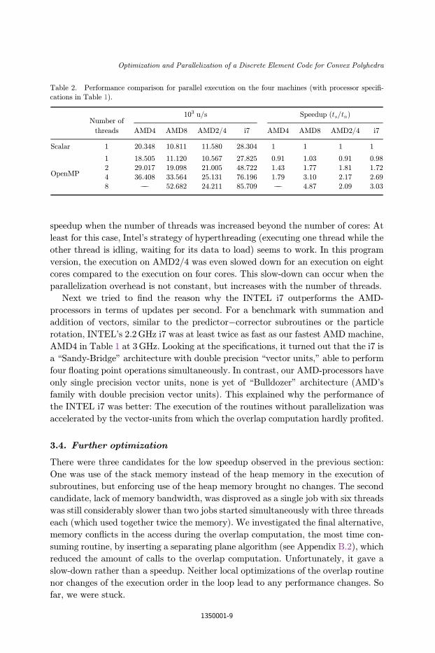
speedup when the number of threads was increased beyond the number of cores: At

least for this case, Intel's strategy of hyperthreading (executing one thread while the

other thread is idling, waiting for its data to load) seems to work. In this program

version, the execution on AMD2/4 was even slowed down for an execution on eight

cores compared to the execution on four cores. This slow-down can occur when the

parallelization overhead is not constant, but increases with the number of threads.

Next we tried to ¯nd the reason why the INTEL i7 outperforms the AMD-

processors in terms of updates per second. For a benchmark with summation and

addition of vectors, similar to the predictor�corrector subroutines or the particle

rotation, INTEL's 2.2GHz i7 was at least twice as fast as our fastest AMD machine,

AMD4 in Table 1 at 3GHz. Looking at the speci¯cations, it turned out that the i7 is

a \Sandy-Bridge" architecture with double precision \vector units," able to perform

four °oating point operations simultaneously. In contrast, our AMD-processors have

only single precision vector units, none is yet of \Bulldozer" architecture (AMD's

family with double precision vector units). This explained why the performance of

the INTEL i7 was better: The execution of the routines without parallelization was

accelerated by the vector-units from which the overlap computation hardly pro¯ted.

3.4. Further optimization

There were three candidates for the low speedup observed in the previous section:

One was use of the stack memory instead of the heap memory in the execution of

subroutines, but enforcing use of the heap memory brought no changes. The second

candidate, lack of memory bandwidth, was disproved as a single job with six threads

was still considerably slower than two jobs started simultaneously with three threads

each (which used together twice the memory). We investigated the ¯nal alternative,

memory con°icts in the access during the overlap computation, the most time con-

suming routine, by inserting a separating plane algorithm (see Appendix B.2), which

reduced the amount of calls to the overlap computation. Unfortunately, it gave a

slow-down rather than a speedup. Neither local optimizations of the overlap routine

nor changes of the execution order in the loop lead to any performance changes. So

far, we were stuck.

Table 2. Performance comparison for parallel execution on the four machines (with processor speci¯-

cations in Table 1).

Number of103 u/s Speedup (ts=tn)

threads AMD4 AMD8 AMD2/4 i7 AMD4 AMD8 AMD2/4 i7

Scalar 1 20.348 10.811 11.580 28.304 1 1 1 1

OpenMP

1 18.505 11.120 10.567 27.825 0.91 1.03 0.91 0.98

2 29.017 19.098 21.005 48.722 1.43 1.77 1.81 1.72

4 36.408 33.564 25.131 76.196 1.79 3.10 2.17 2.698 �� 52.682 24.211 85.709 �� 4.87 2.09 3.03


1350001-9

A problem for the performance analysis was that the compiler substituted library

functions for the original FORTRAN source code. What turned up in the time

pro¯les were the undocumented names of the library functions, which were di±cult

to associate with the part of the source code they represented. For the AMD-pro-

cessors in Table 1, the PGPROF-tool indicated 20% of the total CPU-time as barrier

time (for synchronizing parallel threads). This is close to the percentage for which

unparallelized routines would give the e±ciencies in Table 2 according to Amdahls

law. We concluded that the PGPROF-tool misreported unparallelized routines as

barrier time, and indeed, the barrier time was reduced when we inserted the OMP-

pragmas into up to now not parallelized routines, which will be discussed in the next

sections.

4. Second Approach: Parallelization of Everything Else

4.1. New parallel version

Due to the lack of detailed pro¯ling information, we decided to parallelize all

subroutines. First we parallelized the updates of the particle geometries and the

inertia tensors. Fusing the force and torque computation subroutine compute

all force torque with the loop for the overlap computation in Fig. 5, instead of

running an independent loop (Fig. 4) allowed to transfer the data with a linear

instead of a two-dimensional array. The connectivity-tables for the features were

rewritten from full matrices to sparse matrix form to reduce the memory throughput

per particle. While originally, we had used the same (too large) dummy size for the

maximum numbers of corners and faces for the overlap polyhedron as well as for the

particles for the previous program version, we replaced the dimension with the exact

number of corners and faces to reduce memory throughput.

Fig. 5. Pseudocode of the parallelization of the overlap and force computation of the previous program:The overlap and the forces and torques are computed in the same loop, the overlap geometry is trans-

ferred private local data, in contrast to the old version in Fig. 4, where the data were transferred via a

shared array between two separate loops. \&" stands for continuation line.


1350001-10

We also modi¯ed the force summation from a scalar (Fig. 6) to a parallel version

(see Fig. 7). To use the cache more e±ciently, both in the scalar and parallelized

codes, we sorted the contact list according to the ¯rst particle index, so that the data

for the same particle can be reused for di®erent interaction pairs within a single load

Fig. 6. Pseudocode for scalar force summation in a single loop as used in Sec. 3: The indirect addressing ofthe particle indices p1, p2 allows no parallel execution due to possible dependencies.

Fig. 7. Pseudocode for the parallelizable force summation using two loops: In the ¯rst loop, each thread

sums the forces acting on the particles into its private data array independently. This is followed by a loop

which sums the forces and torques from the independent private tables into a single data array.


1350001-11

operation. To avoid data racing (where reading and writing operations occur on the

same data, so that it is not clear what is read, the old or the modi¯ed values) each

thread has its own temporary variable for the total force (Fig. 7).

Our neighborhood algorithm in Appendix A does not need the tree-structures

which are mentioned in Bara®17 for sort-and-sweep algorithms. The conditions that

particle pairs are entered into the contact list in x-, y- and z-direction are di®erent

and independent. Therefore, the corresponding three subroutines can be called in-

dependently on di®erent threads. Such a coarse-grained parallelism which can assign

di®erent threads to di®erent subroutines is supported in OpenMP via the parallel

sections-construct.20

The results for the newly optimized algorithm can be seen in Table 3: Overall

performance in terms of updates/s is increased by a factor of 1.5 or more, though the

speedup for the i7 has become smaller. For two threads on two processors, the

AMD2/4 exhibits a freak speedup larger than 100%, which can happen on cache-

based machines when the performance on a single core is impaired by cache misses.

The e®ect was signi¯cantly larger than the usual °uctuations in the pro¯les, timings

inside the program and from the operating system were consistent. The other AMD-

machines with multiple cores on a single processor did not show similar e±ciencies.

Though beyond four threads the e±ciency drops, there is still a gain in updates per

second. The reason why no higher speedups are obtained is the neighborhood routine,

which is parallelized via the parallel sections-construct for up to three threads,

irrespective of the available number of threads: As this makes it the only routine with

a computational e®ort O(# of particles) for which not all threads are used, the

overhead is considerable. A more ¯ne-granular parallelization is in preparation.

4.2. Comparison with other codes

Hardly any codes have been completed for discrete element methods for elastic

polyhedral particles. For the \contact dynamics" algorithm for polyhedral particles21

there are no overlaps to compute, only contacts. Moreover, it simulates rigid parti-

cles, which means physically the limit of vanishing strain or external forces. As whole

classes of problems (i.e. sound propagation, which is in¯nity for rigid packings)

Table 3. Performance comparison for the four machines after parallelization of most subroutines with O(number of particles) for 682 particles.

Number of103 u/s Speedup (ts=tn)

threads AMD4 AMD8 AMD2/4 i7 AMD4 AMD8 AMD2/4 i7

Scalar 1 29.847 22.189 17.206 43.837 1 1 1 1

OpenMP

1 28.163 21.701 15.865 41.688 0.94 0.98 0.92 0.952 48.746 37.277 36.556 65.489 1.63 1.68 2.12 1.49

4 83.207 69.761 60.810 85.400 2.79 3.14 3.53 1.95

8 �� 117.419 88.669 73.923 �� 5.29 5.15 1.69


1350001-12

cannot be simulated with contact mechanics, a comparison with our code is not

meaningful. About the code by Muth22 we could not obtain enough information for a

meaningful comparison. To our knowledge, the only other polyhedral DEM, about

which details have been published,23�25 computes the contact force via the distances

of the contact points from the separating plane, and uses a spring constant (units

[N/m]) instead of the Young's modulus which would be a more appropriate pa-

rameter for the elasticity in three dimensions. The performance analysis of the code23

was fragmentary, with reported speedups on an IBM pSeries 690 of 5.2 with eight

threads and on a SGI Altix of 3.4 with 16 threads for merely a thousand time-steps.

The maximal updates per second of simulations of 17 176 particles are about

58.5 � 103 u/s for parallel execution, but details on the architectures and the number

of threads used are missing.

For comparison, we prepared a large system with 17 942 particles, as shown in

Fig. 8. The drum is again formed by 34 particles, with inner diameter 500mm, outer

diameter 560mm and rotates with �=6 rad/s. The grain particles are of ellipsoidal

shape, as the small system. In reference runs with particles of di®erent shape dis-

persion, the update per second rates did not change. With the platforms in Table 1,

the performance results are summarized in Table 4. As is seen, better performance

can be obtained on our platforms and the highest amount of updates per second is

achieved on the i7 machine with eight threads. Considering that the particles we used

Fig. 8. A large drum (upper half not drawn, in decimeter scale) with 17 908 ellipsoidal particles during

simulation and inset with enlargement of the particles. The quadrilateral faces of the prisms forming the

walls are decomposed into triangles.


1350001-13

have almost twice the number of corners and three times of the number of faces as

those used in Ref. 23, we may conclude that our code is more e±cient.

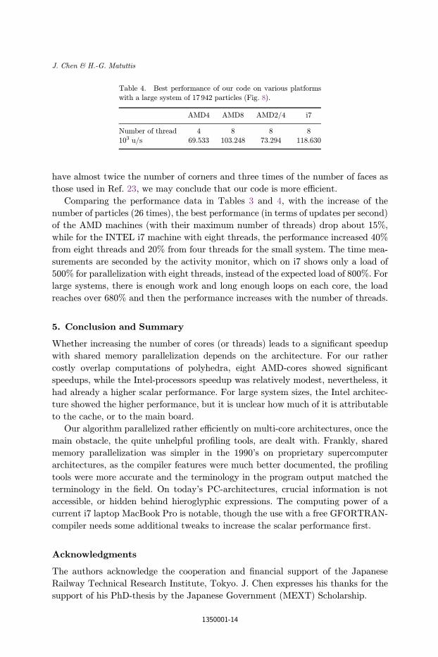
Comparing the performance data in Tables 3 and 4, with the increase of the

number of particles (26 times), the best performance (in terms of updates per second)

of the AMD machines (with their maximum number of threads) drop about 15%,

while for the INTEL i7 machine with eight threads, the performance increased 40%

from eight threads and 20% from four threads for the small system. The time mea-

surements are seconded by the activity monitor, which on i7 shows only a load of

500% for parallelization with eight threads, instead of the expected load of 800%. For

large systems, there is enough work and long enough loops on each core, the load

reaches over 680% and then the performance increases with the number of threads.

5. Conclusion and Summary

Whether increasing the number of cores (or threads) leads to a signi¯cant speedup

with shared memory parallelization depends on the architecture. For our rather

costly overlap computations of polyhedra, eight AMD-cores showed signi¯cant

speedups, while the Intel-processors speedup was relatively modest, nevertheless, it

had already a higher scalar performance. For large system sizes, the Intel architec-

ture showed the higher performance, but it is unclear how much of it is attributable

to the cache, or to the main board.

Our algorithm parallelized rather e±ciently on multi-core architectures, once the

main obstacle, the quite unhelpful pro¯ling tools, are dealt with. Frankly, shared

memory parallelization was simpler in the 1990's on proprietary supercomputer

architectures, as the compiler features were much better documented, the pro¯ling

tools were more accurate and the terminology in the program output matched the

terminology in the ¯eld. On today's PC-architectures, crucial information is not

accessible, or hidden behind hieroglyphic expressions. The computing power of a

current i7 laptop MacBook Pro is notable, though the use with a free GFORTRAN-

compiler needs some additional tweaks to increase the scalar performance ¯rst.

Acknowledgments

The authors acknowledge the cooperation and ¯nancial support of the Japanese

Railway Technical Research Institute, Tokyo. J. Chen expresses his thanks for the

support of his PhD-thesis by the Japanese Government (MEXT) Scholarship.

Table 4. Best performance of our code on various platforms

with a large system of 17 942 particles (Fig. 8).

AMD4 AMD8 AMD2/4 i7

Number of thread 4 8 8 8

103 u/s 69.533 103.248 73.294 118.630


1350001-14

Appendix A. Neighborhood Algorithm via Sort-and-Sweep

Common neighborhood algorithms in molecular dynamics are Verlet-tables and

neighborhood-tables,15 where at certain intervals the whole neighborhood relation

for all particles has to be recomputed from scratch, even if the particles only vibrate

around an equilibrium position, i.e. do not move at all. It is more economic if the

computational e®ort is limited to those particles which change their relative posi-

tion. Both for Verlet- and neighborhood-tables the shape of the cells is independent

of the shape of the particles, so that these algorithm are also very ine±cient for

large size dispersions or elongated particles with arbitrary orientation. Moreover, for

the Cundall�Strack friction model18 and our variant,2 it is necessary to increment

data from a previous time-step for a pair of particles in contact. This is very

inconvenient if we have to search in the list of previous and new pairs whether the

contact existed already in the previous time-step, and which value was registered for

the tangential force. We have therefore implemented the \sort-and-sweep" algo-

rithm,17 which monitors the change of relative positions of extremal coordinates

(\bounding boxes") which we used earlier to simulate systems of very di®erent

particle size in two dimensions.26 A neighborhood list is held for the particle pairs,

into which also additional information (overlap from the previous time-step etc.)

can be included. Changes to this list are only made when sorting of the bounding

box coordinates makes changes necessary due to the relative motion of the particles.

Computer science enjoys discussing sorting algorithms in detail and at length,

generally under the assumption that the lists are not ordered, and the bounds given

are usually worst case bounds. Nevertheless, in our simulation, from one time-step

to the next, our bounding boxes are already partially sorted. On top of that, the

possible changes in the list are rather limited, as particles under elastic interaction

laws cannot move too far, usually only small fractions of their extension in a single

time-step. Therefore, we chose sorting with exchange of neighboring list members

(\Bubble-sort"), as we have to decide the possible interaction anyway on a parti-

cle�particle base, and we have to register the information of possibly contacting

particles into a separate neighborhood list. We do not need more sophisticated

sorting schemes, except for the initialization, where the worst case for Bubble-sort,

an e®ort of Oðn2Þ with n particles would be necessary for an unfavorable chosen

initial con¯guration. As this would lead to an unnecessary delay in reaching the

main loop, we used \Quicksort" for the initial sorting. Additionally, to allow for a

simpler formulation of the if-conditions which compare previous and following

elements in the list, we added a \sentinel" to mark both ends of the list, using the

FORTRAN90 intrinsic function maxval for the maximal double precision value, so

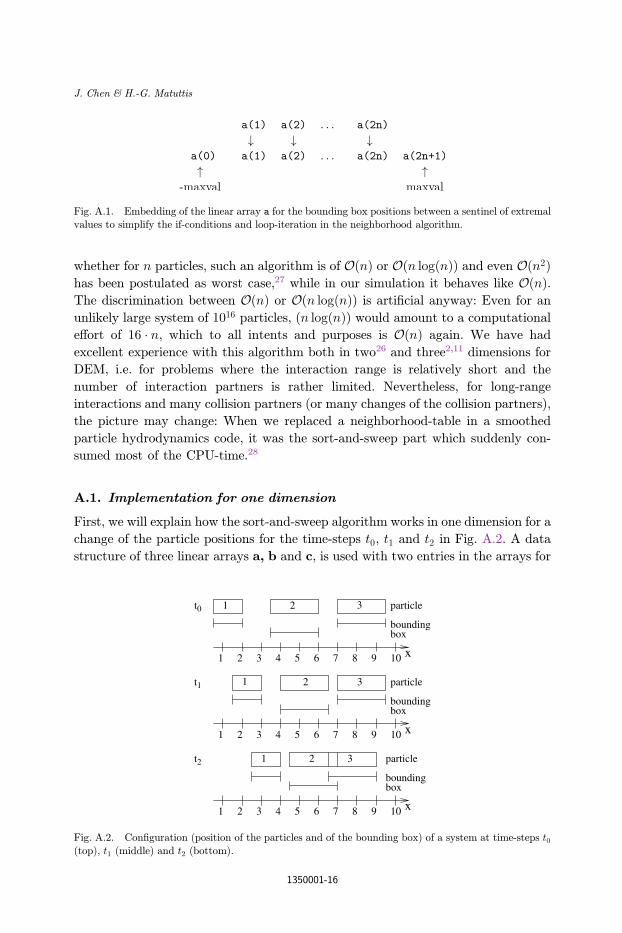
that we have -maxval at the beginning and +maxval at the end. The linear array a

contains then 2nþ 2 elements, 2n of them contain the extremal coordinates of the

particles for each dimensions, which lie between -maxval and +maxval. This sim-

pli¯es the programming, as no additional if-conditions are necessary to prevent

going beyond the list end, see Fig. A.1. There is some discussion in the literature


1350001-15

whether for n particles, such an algorithm is of OðnÞ or O(n logðnÞ) and even Oðn2Þhas been postulated as worst case,27 while in our simulation it behaves like OðnÞ.The discrimination between OðnÞ or O(n logðnÞ) is arti¯cial anyway: Even for an

unlikely large system of 1016 particles, (n logðnÞ) would amount to a computational

e®ort of 16 � n, which to all intents and purposes is OðnÞ again. We have had

excellent experience with this algorithm both in two26 and three2,11 dimensions for

DEM, i.e. for problems where the interaction range is relatively short and the

number of interaction partners is rather limited. Nevertheless, for long-range

interactions and many collision partners (or many changes of the collision partners),

the picture may change: When we replaced a neighborhood-table in a smoothed

particle hydrodynamics code, it was the sort-and-sweep part which suddenly con-

sumed most of the CPU-time.28

A.1. Implementation for one dimension

First, we will explain how the sort-and-sweep algorithm works in one dimension for a

change of the particle positions for the time-steps t0, t1 and t2 in Fig. A.2. A data

structure of three linear arrays a, b and c, is used with two entries in the arrays for

Fig. A.1. Embedding of the linear array a for the bounding box positions between a sentinel of extremalvalues to simplify the if-conditions and loop-iteration in the neighborhood algorithm.

x1 2 3 4 5 6 7 8 9 10

particle

boundingbox

x

1 2

2

1 2 3 4 5 6 7 8 9 10

particle

boundingbox

x

1 2 3

1 2 3 4 5 6 7 8 9 10

particle

boundingbox

t0

t1

t2

3

1 3

Fig. A.2. Con¯guration (position of the particles and of the bounding box) of a system at time-steps t0(top), t1 (middle) and t2 (bottom).


1350001-16

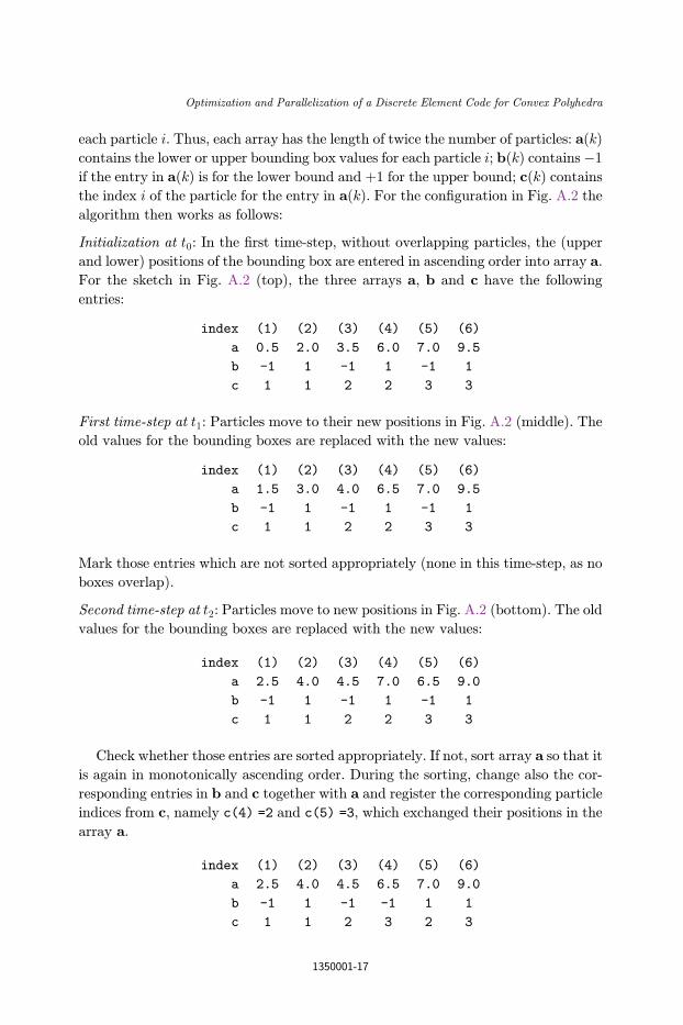
each particle i. Thus, each array has the length of twice the number of particles: a(k)

contains the lower or upper bounding box values for each particle i; b(k) contains �1

if the entry in a(k) is for the lower bound and þ1 for the upper bound; c(k) contains

the index i of the particle for the entry in a(k). For the con¯guration in Fig. A.2 the

algorithm then works as follows:

Initialization at t0: In the ¯rst time-step, without overlapping particles, the (upper

and lower) positions of the bounding box are entered in ascending order into array a.

For the sketch in Fig. A.2 (top), the three arrays a, b and c have the following

entries:

index (1) (2) (3) (4) (5) (6)

a 0.5 2.0 3.5 6.0 7.0 9.5

b -1 1 -1 1 -1 1

c 1 1 2 2 3 3

First time-step at t1: Particles move to their new positions in Fig. A.2 (middle). The

old values for the bounding boxes are replaced with the new values:

index (1) (2) (3) (4) (5) (6)

a 1.5 3.0 4.0 6.5 7.0 9.5

b -1 1 -1 1 -1 1

c 1 1 2 2 3 3

Mark those entries which are not sorted appropriately (none in this time-step, as no

boxes overlap).

Second time-step at t2: Particles move to new positions in Fig. A.2 (bottom). The old

values for the bounding boxes are replaced with the new values:

index (1) (2) (3) (4) (5) (6)

a 2.5 4.0 4.5 7.0 6.5 9.0

b -1 1 -1 1 -1 1

c 1 1 2 2 3 3

Check whether those entries are sorted appropriately. If not, sort array a so that it

is again in monotonically ascending order. During the sorting, change also the cor-

responding entries in b and c together with a and register the corresponding particle

indices from c, namely c(4) =2 and c(5) =3, which exchanged their positions in the

array a.

index (1) (2) (3) (4) (5) (6)

a 2.5 4.0 4.5 6.5 7.0 9.0

b -1 1 -1 -1 1 1

c 1 1 2 3 2 3


1350001-17

Only if a lower bound has moved below an upper bound (this is the case, b(4) =

-1, b(5) = 1), there is a possible overlap between the two particles, so the particle

pair (2, 3) is registered as a new entry in the contact list as candidate for an inter-

action, as in Fig. A.3(a). If a lower bound would move above an upper bound, as in

Fig. A.3(b), nothing would be done. The opening in a contact will be better dealt in a

separate loop over the old contact list, so that pairs of particles which become too far

separated are removed. For the other cases in Fig. A.3, if two lower bounds, in

Figs. A.3(c) and A.3(d), or two upper bounds, like in Figs. A.3(e) and A.3(f) ex-

change positions, the bounding boxes of the two particles remain overlapping as the

previous time-step, and nothing has to be done. As long as bounding boxes overlap,

as in Figs. A.3(c)�A.3(f), we keep a record of the old pairs and update the record by

eliminating those entries which have lost their overlap in a separate loop. Periodic

boundary conditions26 can also be realized: Bounding boxes from the left side of the

system are incremented by the system sizes and copied to the right of the list as

\shadow bounding boxes," and vice versa.

A.2. Implementation for two dimensions

When Bara®17 introduced the neighborhood algorithm via sorting axis aligned

bounding boxes (sort-and-sweep) in one dimension, he did not explicitly say what to

do in higher dimensions and only mentioned tree structures. In principle, in two

dimensions the algorithm works in the same way as in one dimension, except for one

problem shown in Fig. A.4: While the new particle pair (i; j) would enter only once in

the neighborhood list for the x-coordinate in Fig. A.4(a), and in Fig. A.4(b) only once

for the y-coordinate, as in the one-dimensional case, in Fig. A.4(c) it would be

registered twice in the list of possible contacting pairs, both for the x- and the

y-coordinate. Searching for double entries and purging them from the list is incon-

venient. Instead, it is better to use the information about the old bounding boxes in

ticle moves below upper bounding

For all other position changes of the bounding boxes in the list, the neighborhood relation does not change:

ticle moves over upper bounding box of left particle: intersection

Lower bounding−box of right par−

box of left particle: no intersection

Lower bounding−box of right par−

Fig. A.3. Con¯gurations and relative movement of particles (the thinner arrow for the particle in whiteand the thicker arrow for the gray one), those which lead to a possible overlap (a), and those which

separate overlapping particles (b) or which do not change the overlapping situation (c)�(f ).


1350001-18

the previous time-step26 as in the following piece of pseudocode:

(1) If there is a new overlap in the x-direction for the pair (i; j), register it in the

contact list if there is simultaneously an overlap in the y-direction.

(2) If there is a new overlap in the y-direction for the pair (i; j), only register it in the

contact list if there is an overlap of the bounding boxes in the x-direction already

in the previous time-step.

With this scheme, the case in Fig. A.4(a) will be registered in the loop over the

x-coordinates and the case in Fig. A.4(b) will be registered for the position changes of

the bounding boxes along the y-direction, since their bounding boxes along the

x-direction overlapped at the previous time-step. The case in Fig. A.4(c) will be

registered in the loop over the x-direction, not for the y-direction, as there was no

overlap of the two bounding boxes along the x-direction at the previous time-step.

With this scheme, the problem of double entries is dealt with in two dimensions

without additional computational complexity, tree structures or otherwise.

A.3. Implementation for three dimensions

For three dimensions, the situation is analogous to two dimensions, only there are

more cases which may lead to multiple entries in the contact list. The algorithm

works again as in one dimension, except for the following cases: While in Figs. A.5(a)�A.5(c), the new particle pair (i; j) would enter only once in the neighborhood list for

the x-coordinate, and in Figs. A.5(d)�A.5(f) it would enter twice, in Fig. A.5(g) it

would enter even three times. Searching the lists for double or triple entries is even

more inconvenient than in two dimensions. Again we can use the information about

the old bounding boxes in the previous time-step as in the following piece of pseu-

docode:

(1) In the loop for sorting the x-direction, if there is a new overlap in the x-direction

for the pair (i; j), immediately register it in the contact list if there is simulta-

neously an overlap in the y- and z-direction.

(2) In the loop for sorting the y-direction, if there is a new overlap in the y-direction

for the pair (i; j) and simultaneously an overlap in the x- and z-direction, only

register it in the contact list if there was an overlap in the bounding boxes in the

x-direction already in the previous time-step.

i

j

(a)

i

j

(b)

i

j

(c)

Fig. A.4. Relative movement of bounding-boxes in two dimensions: New overlap in x-direction (a), new

overlap in y-direction (b), and new overlap both in x- and y-directions (c).


1350001-19

(3) In the loop for sorting the z-direction, if there is a new overlap found in

the z-direction for the pair (i; j) and simultaneously an overlap in the x- and

y-direction, only register it in the contact list if there was an overlap in the

bounding boxes in the x- and y-direction already in the previous time-step.

Applying this scheme to Fig. A.5, we ¯rst check the new overlaps along the

x-direction, Figs. A.5(a), A.5(e)�A.5(g), and record all of the pairs immediately in

the loop for the x-direction. We then check the new overlaps along the y-direction for

Figs. A.5(b), A.5(d), A.5(e) and A.5(g): In the loop for the y-direction, Figs. A.5(b)

and A.5(d) are registered since they have overlaps of the bounding boxes in

x-direction at the previous time-step while Figs. A.5(e) and A.5(g) are excluded

for not having overlaps. Lastly, we check the new overlaps along z-direction for

Figs. A.5(c)�A.5(g): only Fig. A.5(c) is registered for having overlaps both in x- and

y-directions at the previous time-step; Figs. A.5(d) and A.5(e) are not registered, as

they had no overlap in either x- or y-direction and (g) did not have an overlap in both

x- and y-directions at the previous time-step. It is clear that with this scheme, no

double (or triple) entry of pairs would occur in three dimensions. In principle, the

subroutines for the computation of the contact list for the x-, y- and z-direction via

sorting can be computed independently and in parallel. From the point of load-

balancing it should be noted that the loop for the y-component has to execute more

comparisons than the loop for the x-component, and the loop for the z-component

has to execute more comparisons than the loop for the y-component. The number of

(a) (b) (c) (d)

(e) (f) (g)

Fig. A.5. Relative movement of bounding boxes in three dimensions where the overlap candidate pairs

would only be entered once (a�c), twice (d�f) and three times (g) if no precautions are taken.


1350001-20

data which has to be dealt with (bounding boxes from the previous time-step) also

increases for the loops in y- and z-direction.

Appendix B. Re¯nement of the Contact List

For polyhedra, overlapping bounding boxes are just a \rough" estimate for a pos-

sible overlap, they are \exact" only for cuboids with sides oriented parallel to the

axes. To reduce the calls for the full computation of the overlap polyhedron, the

elimination of pairs of particles which certainly are not in contact is desirable to

reduce the computational e®ort. In two dimensions,10 using circles around the

center-of-mass was quite useful to eliminate pairs of nonintersecting particles. Un-

fortunately, in three dimensions, with ellipsoidal outlines in our simulation, this

approach is totally ine®ective, as for most particles the bounding spheres intersect

together with the bounding boxes. Generalizing the bounding spheres to bounding

ellipsoid makes no sense, for computing the possible intersection of general ellipsoids

needs the solution of a generalized eigenvalue problem for 4� 4 matrices, which

would be at least as numerically unstable as its two-dimensional equivalent29

for ellipses. In the sort-and-sweep algorithm, only the coordinate-aligned bound-

ing boxes are used, while for faces with normals � 45� inclination towards the axes,

particles will often not overlap when their bounding boxes do. Therefore, we re¯ne

the contact list by using the projections of the corners of the connecting line be-

tween the centers of mass of the particles to obtain additional information which is

independent of the orientation of the coordinate axes. In the following, we use

¯gures of polygons in two dimensions to explain the algorithms for the corre-

sponding polyhedra in three dimensions. While the original contact list obtained

from the bounding boxes must be retained as it is, as the sort-and-sweep algorithm

takes into account only changes of neighborhoods, a list of less pairs will be passed

for the computation of the overlap polyhedron, which will be referred to as \reduced

contact list."

B.1. Re¯nement via projection of the extremal vertices

With the projection, the protrusions of the vertices of the two particles along the line

connecting their centers-of-mass are compared, see Fig. B.1 for the two-dimensional

analogue. For two polyhedra, P1 and P2, with the centers-of-mass as c1 and c2, the

algorithm is:

(1) Compute the unit base vector from c1 to c2: (c2-c1)/jjc2-c1jj.(2) Compute the projections of the vertices of P1 and of P2 onto the unit base vector.

(3) Find the maximal projection of P1 (max projection P1); Find the minimal

projection of P2 (min projection P2).

(4) If max projection P1> min projection P2, keep the particle pair in the

contact list; otherwise remove the pair from the list.


1350001-21

While the computation of the projections for the vertices (vector inner product for

each vertex) needs more computational e®ort than comparing the bounding spheres

(scalar comparison of the radii only once), it can also deal with particles with very

elongated shape, seen Fig. B.1(b).

B.2. Separating planes

When the projection algorithm from the previous section fails to indicate that the

particles are without overlap, the full overlap computation must be performed, but

only in about half the cases, an actual overlap of the polyhedra exists. We therefore

tried to devise an additional algorithm, more costly than the projection re¯nement,

but cheaper than the full overlap computation, to eliminate at least a part of the

overlap-calls. While the algorithm by Zhao and Nezami23,24 needs the separating

plane for each force computation of interacting particles in every case, to reduce our

contact list, we can make do with a \quick and dirty" approach which at least

eliminates some of the pairs, as long as time is saved compared to a full overlap

computation. Our algorithm for two polyhedra of P1 and of P2 with centers c1 and

c2, is the following:

(1) Compute the ¯rst plane, with the normal parallel to the connection of the centers

of mass c1 and c2:

(2) Compute the distance of the vertices of the polyhedra P1 and of P2 from the

normal plane.

(3) If there cannot be an overlap due to the relative distance of the vertices of P1 and

of P2 to the plane, the plane is the separating plane; Exit.

projectionof P2

minimal

projectionof P1

maximal

c

c

1

2

(a)

projectionof P1

maximal

projectionof P2

minimalc2

c1

(b)

Fig. B.1. Re¯nement of the contact detection results via projection in two dimensions: (a) Overlap of theminimal projection of polygon P1 and the maximal projection of polygon P2, this pair is kept in the contact

particle pair list; (b) No overlap of the minimal projection of polygon P1 and the maximal projection of

polygon P2, this pair is removed from the reduced contact list which is passed to the computation of the

overlap polyhedron.


1350001-22

(4) Choose those vertices v1;v2 of P1 and P2 which protrude furthest beyond the

current plane towards the other polyhedron.

(5) Choose the new separation plane with the normal Ni in the middle between v1

and v2.

(6) Goto 4.

Additionally, one has to limit the number of iterations to avoid an in¯nite loop

when the polyhedra actually overlap. As test case, we used convex hulls, which are

much more irregular than the ellipsoid-tessellations in our simulations, as a worst

case scenario. For pairs of convex hulls over 16 unit random numbers, shifted by

(0;�0:4; 0), the bounding boxes always overlapped in at least one coordinate. In that

case, about 50% of the separating planes are found with the initial plane, 18% are

found after one iteration, about 3% after two and about 1.25% after three and four

iterations, so in 72% of the cases, a separating plane is detected. As 76% of the pairs

have no overlap at all, our algorithm was able to detect 95% of those cases, the

bounding box algorithm indicates a possible interaction but there is no particle

overlap.

References

1. H.-G. Matuttis, S. Luding and H. Herrmann, Powder Technol. 109, 278 (2000).2. J. Chen and H.-G. Matuttis, NCTAM Japan, J. Phys. Soc. Jpn 60, 225 (2011).3. S. A. E. Shourbagy, S. Morita and H. G. Matuttis, J. Phys. Soc. Jpn. 75, 104602 (2006).4. D. E. Wolf, Modeling and computer simulation of granular media, in Computational

Physics: Selected Methods, Simple Exercises, Serious Applications, eds. K. H. Ho®mannand M. Schreiber (Springer, 1996), pp. 64�95.

5. T.-T. Ng, Numerical simulations of granular soil using elliptical particles, in Micro-structural Characterization in Constitutive Modeling of Metals and Granular Media:Presented at the ASME Summer Mechanics and Materials Conferences, ASME, Rot-terdam/Brook¯eld, April 28�May 1, 1992.

6. C. Thornton, Kona Powder and Particle Journal 15, 81 (1997).7. J. Katagiri, T. Matsushima and Y. Yamada, Dense granular °ow simulation for irregu-

larly-shaped grains by image-based DEM, in Proc. of the 57th National Congress ofTheoretical and Applied Mechanics (2008), pp. 511�512.

8. J. Chen, Discrete element method for 3D simulations of mechanical systems of non-spherical granular materials, PhD thesis, The University of Electro-Communications(2012).

9. D. Negrut, A. Tasora, H. Mazhar, T. Heyn and P. Hahn, Multibodynam. Syst. Dynam.27, 95 (2012).

10. H. G. Matuttis, Granular Matter 1, 83 (1998).11. J. Chen, A. Schinner and H.-G. Matuttis, NCTAM Japan, J. Phys. Soc. Jpn 59, 335

(2010).12. D. Gove, Multicore Application Programming: For Windows, Linux, and Oracle Solaris

(Addison-Wesley, 2010).13. E. Hairer and G. Wanner, Solving Ordinary Di®erential Equations II Sti® and Di®er-

ential-Algebraic Problems, 2nd revised edn. (Springer, 1996).


1350001-23

14. C. W. Gear, Numerical Initial Value Problems in Ordinary Di®erential Equations(Prentice-Hall, 1971).

15. M. P. Allen and D. J. Tildesley, Computer Simulation of Liquids (Clarendon Press,Oxford, 1987).

16. P. Jim�enez, F. Thomas and C. Torras, Comput. Graphics 25, 269 (2001).17. D. Bara®, An introduction to physically based modeling: Rigid body simulation II ��

nonpenetration constraints, in Siggraph Course Notes (1997), pp. D31�D68, http://www.cs.cmu.edu/�bara®/sigcourse/.

18. P. A. Cundall and O. D. L. Strack, Geotechnique 29, 47 (1979).19. C. L. Lawson, R. J. Hanson, D. Kincaid and F. T. Krogh, ACM Trans. Math. Softw. 5,

308 (1979).20. B. Chapman, G. Jost and R. van der Pas, Using OpenMP: Portable Shared Memory

Parallel Programming (MIT Press, 2007).21. E. Az�ema, F. Radjai, R. Peyroux, V. Richefeu and G. Saussine, Eur. Phys. J. E 26, 327

(2008).22. B. Muth, G. Of, P. Eberhard and O. Steinbach, Arch. Appl. Mech. 77, 503 (2007).23. D. Zhao, Three-dimensional discrete element simulation for granular materials, PhD

thesis, University of Illinois at Urbana-Champaign (2006).24. E. G. Nezami, Three-dimensional discrete element simulation of granular materials using

polyhedral particles, PhD thesis, University of Illinois at Urbana-Champaign (2007).25. E. G. Nezami, Y. M. Hashash, D. Zhao and J. Ghaboussi, Int. J. Numer. Anal. Methods

Geomech. 31, 1147 (2007).26. N. K. Mitani, H.-G. Matuttis and T. Kadono, Geophys. Res. Lett. 31, L15606 (2004).27. B. C. Vemuri, L. Chen, L. Vu-Quoc, X. Zhang and O. Walton, Graph. Models Image

Process. 60, 403�422 (1998).28. K. Takiguchi, Flow simulation with the smoothed particle method, Master's thesis, The

University of Electro-Communications (2010) (in Japanese).29. H.-G. Matuttis, N. Itô, H. Watanabe and K. M. Aoki, Vectorizable overlap computation

for ellipse-based discrete element method, in Powders and Grains, ed. Y. Kishino(Balkema, Rotterdam, 2001), pp. 173�176.


1350001-24

optimization and openmp parallelization of …€¦ · optimization and openmp parallelization of a...

Documents