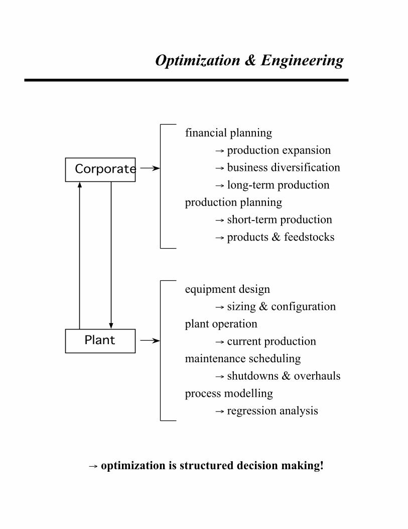
Optimization & Engineering

→ optimization is structured decision making!

Corporate

Plant

financial planning→ production expansion→ business diversification→ long-term production

production planning→ short-term production→ products & feedstocks

equipment design→ sizing & configuration

plant operation→ current production

maintenance scheduling→ shutdowns & overhauls

process modelling→ regression analysis

Introductory Example

Problem:

Schedule your activities for next week-end, given youonly have $100 to spend.

Question:

How can we go about solving this problem in a coherent fashion?

Introductory Example

A systematic approach might be:

Step 1:Choose a scheduling objective.

Step 2:List all possible activities and pertinent informationregarding each activity,

activity fun units / hrFi

CostCi

time limitsLi

Introductory Example

Step 3:Specify other limitations.

tavailable =$available =

Step 4:Decide what the decision variables are.

Step 5:Write down any relationships you know of among thevariables.

Introductory Example

Step 6:Write down all restrictions on the variables.

Step 7:Write down the mathematical expression for the objective.

Introductory Example

Step 8:Write the problem out in a standard form.

There is a more compact way to write this problem down.⇒ matrix-vector form.

General Form of an Optimization Problem

ul

ul

),(

= ),(

:subject to

,

), P(optimize

uuu

xxx

0uxg

0uxf

ux

ux

!!

!!

!

x u decision variables model

variables.independent dependentexternal internaldegrees of freedom tearnonbasic basic

inequality constraintsoperating constraints

boundslimits

objective functionperformance functionprofit (cost) function

equality constraintsprocess model

Development Stages of Optimization Problems

1) Problem Definition:→ objectives,

• goal of optimization.• performance measurement.

→ process models,• assumptions & constants.• equations to represent relationships,

- material / energy balances,- thermodynamics,- kinetics, etc.

• constraints and bounds to represent limitations,- operating restrictions,- bounds / limits.

2) Problem Formulation:→ standard form,→ degrees of freedom analysis,

• over-, under- or exactly specified?• decision variables (independent vs. dependent).

→ scaling of variables,• units of measure.• scaling factors.

Development Stages for Optimization Problems

3) Problem Solution:→ technique selection,

• matched to problem type,• exploit problem structure,• knowledge of algorithms strengths & weaknesses.

→ starting points,• usually several and compare.

→ algorithm tuning,• termination criteria,• convergence tolerances.• step length.

4) Results Analysis→ solution uniqueness,→ perturbation of optimization problem,

• effects of assumptions,• variation (uncertainty) in problem parameters,• variation in prices / costs.

Development Stages for Optimization Problems

4) Results Analysis 3) Solution

1) Definition 2) Formulation

Solving an optimization problem isiterative!

Solution of an optimization problem requires all of the steps:• a full understanding is developed by following the complete cycle,• good decisions require a full understanding of the problem,• shortcuts lead to bad decisions.

Modelling Example

Consider the binary distillation column at steady-stateoperation:

Question:How can we model this process unit?

F,XF

D,XDR

L,XL

QC

QR

p

(5 ideal stages)

Modelling Example

1) What is the modelling goal?→ predict over-head product flow and composition as

accurately as possible.

2) What physical phenomena are occuring in the process?→ vapour-liquid equilibrium.→ heat transfer.

3) What physical laws must be obeyed by the process?→ conservation of mass.→ conservation of energy.→ conservation of component species (no reaction).

4) What assumptions can we make?→ only two species present (XA + XB = 1).→ complete condensation in condenser.→ heat losses are negligible.→ equimolal over-flow (ΔHvap the same for both species).→ feed is all liquid at temperature of feed tray.→ constant relative volatility.

Modelling Example

Our model equations consist of:

1) material balances,

F = L+DXFF = XLL+XDD

qvapour = R+D

2) energy balances,

QR = QC

QR = ΔHvap qvapour

QC = ΔHvap qvapour

mass balance

component balance

internal vapour flow

energy balance

creation and condensation of internal vapour flow

Modelling Example

How will we represent the vapour-liquid equilibria withinthe column?

Some possibilities:

• Fenske-Eduljee• Smoker’s• McCabe-Thiele

- tray-by-tray material balances.• Ponchon-Savarit

- tray-by-tray material and energy balances.

Since we want an accurate model, but do not have thenecessary detailed thermodynamic information for each oftrays, let’s try McCabe-Thiele.

Then for each ideal tray we will need:

1) component balance.2) a vapour-liquid equilibrium expression.

Modelling Example

3) tray balances (numbering from the column top),

R (XD - X1) = qvapour (XD -Y2)R (X1 - X2) = qvapour (Y2 - Y3)

F XF + R X2 - (F+R) X3 = qvapour (Y3 - Y4)

(F+R) (X3 - X4) = qvapour (Y4 - Y5)

(F+R) X4 - LXL = qvapour Y5

4) vapour-liquid equilibria,

(1 + (α - 1) * X1) * XD = α * X1

(1 + (α - 1) * X2) * Y2 = α * X2

(1 + (α - 1) * X3) * Y3 = α * X3

(1 + α - 1) * X4) * Y4 = α * X4

(1 + α - 1) * XL) * Y5 = α * XL

stripping section

enriching section

feed tray

reboiler

Modelling Example

Thus, our model is:

F - L - D = 0 XFF - XLL - XDD = 0

qvapour - R - D = 0

QR - QC = 0 QR - ΔHvap qvapour = 0 QC - Δ Hvap qvapour = 0

R (XD - X1) - qvapour (XD -Y2) = 0 R (X1 - X2) - qvapour (Y2 - Y3) = 0F XF + R X2 - (F+R) X3 - qvapour (Y3 - Y4) = 0 (F+R) (X3 - X4) - qvapour (Y4 - Y5) = 0 (F+R) X4 - LXL - qvapour Y5 = 0

(1 + (α - 1) * X1) * XD - α * X1 = 0 (1 + (α - 1) * X2) * Y2 - α * X2 = 0 (1 + (α - 1) * X3) * Y3 - α * X3 = 0 (1 + (α - 1) * X4) * Y4 - α * X4 = 0 (1 + (α - 1) * XL) * Y5 - α * XL = 0

Then for our steady-state binary distillation column:

Goal:Increase distillate flowrate while maintaining purity.

Questions:What process variables can we independently changeto improve operation?

An Engineering Example

F,XF

D,XDR

L,XL

QC

QR

p

To determine the degrees of freedom (the number of variableswhose values may be independently specified) in our modelwe could simply count the number of independent variables(the number of variables which remain on the right- hand side)in our modified equations.

This suggests a possible definition:

degrees of freedom = # variables - # equations

Definition:

The degrees of freedom for a given problem are thenumber of independent problem variables which mustbe specified to uniquely determine a solution.

In our distillation example, there are:16 equations16 variables (recall that F and XF are fixed by

upstream processes).

This seems to indicate that there are no degrees of freedom.

Degrees of Freedom

Degrees of Freedom

Consider the three equations relating QC, QR, and qvapour:

QR - QC = 0 QR - ΔHvap qvapour = 0 QC - ΔHvap qvapour = 0

Notice that if we subtract the last from the second equation:

QR - ΔHvap qvapour = 0 - QC - ΔHvap qvapour = 0

QR - QC = 0

the result is the first equation.

It seems that we have three different equations, which containno more information than two of the equations. In fact any ofthe equations is a linear combination of the other twoequations.

We require a clearer, more precise definition for degrees offreedom.

Degrees of Freedom

A More Formal Approach:

Suppose we have a set of "m" equations:

h(v) = 0

in the set of variables v ("n+m" elements). We would like todetermine whether the set of equations can be used to solve forsome of the variables in terms of the others.

In this case we have a system of "m" equations in "n+m"unknown variables. The Implicit Function Theorem states thatif the "m" equations are linearly independent, then we candivide our set of variables v into "m" dependent variables uand "n" independent variables x:

The Implicit Function Theorem goes on to give conditionsunder which the dependent variables u may be expressed interms of the independent variables x or:

u = g(x)

Degrees of Freedom

Usually we don't need to find the set of equations u = g(x), weonly need to know if it is possible. Again the Implicit FunctionTheorem can help us out:

if rank [∇vh ] = m , all of the model equations arelinearly independent and it is possible (at least in theory)to use the set of equations h(v) = 0 to determine valuesfor all of the "m" dependent variables u given values forthe "n" independent variables x.

Alternatively we could say that the number of degrees offreedom in this case are the number of independent variables.(Recall that there are "n" variables in x).

We know that: rank [∇vh ] ≤ m.

What does it mean if:rank [∇vh ] < m?

degrees of freedom = number of variables - number of linearly independent equations

Degrees of Freedom

In summary, determination of the degrees of freedom for aspecific steady-state set of equations requires:

1) determination of rank [∇vh].

2) if rank [∇vh] =number of equations (m), then all ofthe equations are linearly independent and:

d.o.f. = # variables - # equations.

3) if rank [∇vh] <number of equations (m), then all ofthe equations are not linearly independent and:

d.o.f. = # variables - rank [∇vh].

Remember:For sets of linear equations, the analysis has to be performedonly once. Generally, for nonlinear equation sets, the analysisis only valid at the variable values used in the analysis.

Degrees of Freedom

Degrees of freedom analysis tells us the maximum number ofvariables which can be independently specified to uniquelydetermine a feasible solution to a given problem.

We need to consider degrees of freedom when solving manydifferent types of problems. These include:

i) plant design,ii) plant flowsheeting,iii) model fitting,

and, of course, optimization problems.

Modelling Problem

The file “distill.m” contains the distillation column modeldiscussed in this section of the course. Using Matlab’s“fsolve” command to investigate:

a) The effect of changes in column feed-rate on overheadcomposition and draw-rate,

b) The effect of column feed composition on overheadcomposition and draw-rate,

c) The effect of changes in relative volatility on overheadcomposition and draw-rate,

Classifying Optimization Problems

nonlinear

problem

Mixed-Integer LinearProgramming (MILP)

LinearProgramming (LP)

Non-LinearProgramming (NLP)

Mixed-Integer Non-Linear Programming (MINLP)

StochasticProgramming (SP)

stochastic

continuity

deterministic

discrete

linear

linear

nonlinear

nonlinear

linearconstraints?

linearobjective?

linear

linear

nonlinear

continuous

linearobjective?

linearconstraints?

objective

constraints Semi-DefiniteProgramming (SDP)

Multi-GoalProgramming (MGP)

vector scalar

vector matrix

Classifying Optimization Problems

This workshop will focus on:

→ objective functions which are continuouslydifferentiable in the variables,

→ constraint equations which are continuouslydifferentiable in the variables.

Optimization problems with scalar objective functions andvector constraints can be classified:

objective function

constraints problemtype

linear

nonlinear

linear

nonlinear

linear

linear

nonlinear

nonlinear

LP

NLP

NLP

NLPmostdifficult

LP - linear programmingNLP - nonlinear programming