Optimization Models for Shale Gas Water Management

Linlin Yang†, Jeremy Manno‡ and Ignacio E. Grossmann†∗

†Department of Chemical Engineering, Carnegie Mellon University, Pittsburgh, PA

‡Carrizo Oil & Gas, Houston, TX

May, 2014

Abstract

There are four key aspects for water use in hydraulic fracturing, including source water acquisition, wastewater

production, reuse and recycle, and subsequent transportation, storage, and disposal. This work optimizes water use

life cycle for wellpads through a discrete-time two-stage stochastic mixed-integer linear programming model under

uncertain availability of water. The objective is to minimize expected transportation, treatment, storage, and disposal

cost while accounting for the revenue from gas production. Assuming freshwater sources, river withdrawal data,

location of wellpads and treatment facilities as given, the goal is to determine an optimal fracturing schedule in

coordination with water transportation, and its treatment and reuse. The proposed models consider a long time

horizon and multiple scenarios from historical data. Two examples representative of the Marcellus Shale play are

presented to illustrate the effectiveness of the formulation, and to identify optimization opportunities that can improve

both the environmental impact and economical use of water.

Introduction

With the advancement in directional drilling and hydraulic fracturing, shale gas is predicted to provide 46% of the

United States natural gas supply by 20351. The number of wells drilled in the Marcellus shale play has increased from

112 in 2007 to 1365 in the year 20122. Multiple wells can be drilled from a single wellpad, and this configuration

limits environmental footprint and impact on the surface in comparison to having individual vertical wells with one

well per pad. Development a wellpad involves site preparation, drilling, completion, and production. The timeline is

shown in Figure 1.

Water use is associated with each step of the drilling and production process. Specifically, 90% of water used in

shale gas production is for hydraulic fracturing, while the remaining is necessary during the drilling process. Each

well is injected under high-pressure using a fluid consisting of water, sand, and chemicals to fracture the gas-holding

1

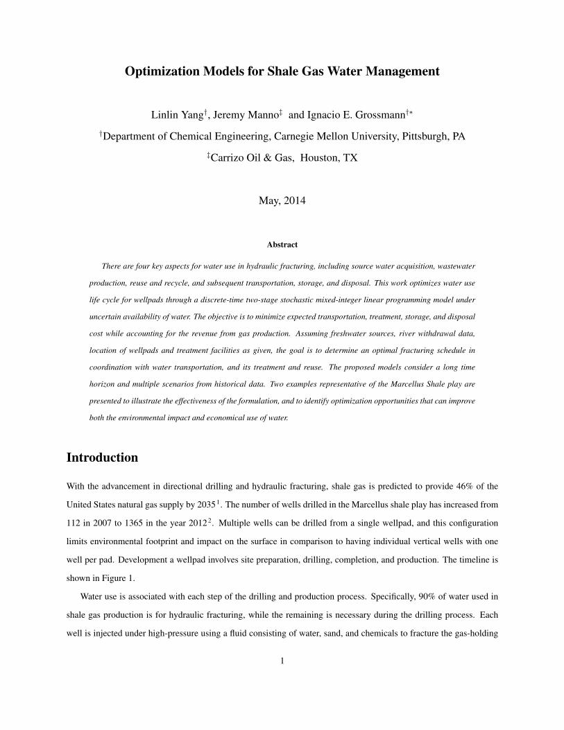
subsurface rock formation. The horizontal portion of the well is fractured, or stimulated, in a number of stages as

shown in Figure 2. Each stage requires a fixed volume of water. Stage 1, which is located near the end of the well, is

stimulated first, then the stage is temporarily plugged to prevent flowback from stage 1. This is followed by stage 2,

and the process is repeated along the full length of the horizontal portion of the well until the last stage is completed.

Typically, each crew can frac at the rate of up to four stages per day. Once all the stages are completed, the well plugs

are drilled through and gas production begins.

The challenge with water use is that a large volume of it is required in a short-period of time. On average, about

19,000-26,000 m3 of water is used to complete each well. A wastewater production forecast for the Marcellus play

suggests that Pennsylvania wells will generate over 15 million m3 per year by 20253. Furthermore, the injected water

that remains underground accounts for 0.3% of all water consumption in the US. Despite the large requirement for

water, the water use per unit energy generated is lower compared to other conventional and unconventional energy

sources as shown in Figure 34. Furthermore, if shale gas is used to generate electricity in a combined-cycle power

plant, the quantity of water consumed per unit of energy generated could be 80% less than that required by a con-

ventional pulverized coal power plant. Even though the Marcellus shale play overlies a water-rich region, regulatory

restrictions pose considerable logistics challenges that demand sophisticated management and logistical strategies.

The steps for water use in shale gas development involves: freshwater acquisition, transportation, injection, treat-

ment, storage, and disposal (the cycle is shown in Figure 4). During the completion phase, freshwater is acquired and

stored in freshwater impoundments. Then sand (8.96%) and chemical additives (0.44%) are added to the water to form

the frac fluid5. Once the plugs are drilled through, there is an initial period when water returns to the surface, which

is called flowback. This is followed by the well’s production period of 20 to 40 years, during which time there is a

small amount of produced water that returns to the surface along with the gas produced. By regulations, wastewater

cannot be stored in freshwater impoundments. Instead, wastewater is stored in frac tanks or specially constructed

impoundments. The flowback and produced water contain various contaminants that need to be treated in order to

partially remove them for recycling and reuse it at the next well.

Shale play logistics such as the sources for freshwater acquisition, storage of water, the volume of water required

to fracture each stage, and the composition and volume of the wastewater vary greatly across geographic sites and

the operational life of a well. Furthermore, since the operation is under state regulations, the permitting processes are

subject to different criteria. For multi-wellpad operations, determining long-term water use logistics is a challenging

problem that can be formulated as a scheduling problem.

In this paper we develop a model that optimizes water-use life cycle for wellpads through a mixed-integer linear

programming (MILP) discrete-time representation. The objective is to minimize the cost of transportation, treatment,

2

storage, and disposal while also accounting for the revenue of gas production within the specified time horizon. This

time horizon must be at least one year to capture the seasonal availability of water. Assuming that freshwater sources,

river withdrawal data, location of wellpads and treatment facilities are given, the goal is to determine an optimal

fracturing schedule and recycling ratio. Since this is a difficult problem to model and solve, we intend to consider as a

first step freshwater acquisition.

The paper is organized as follows. The freshwater handling section accounts for the trade-off between water avail-

ability and freshwater transportation cost, as well as environmental implications of transportation. We next address in

the wastewater handling section the problem that considers the entire economic optimization, including water treat-

ment, storage, disposal, and income from gas production. In each section, relevant background is introduced first,

followed by a general problem statement, its optimization formulation, and an example to illustrate the application of

the optimization model. We focus on applications in the Marcellus Shale play although the proposed models can be

used in other shale gas formations.

Freshwater handling

Background

The conventional sources for water used in hydraulic fracturing includes surface water, ground water, treated wastew-

ater, and cooling water. The most common one is surface water such as lakes or rivers, which typically costs about

$1.76-3.52/m3 in the state of Pennsylvania. On the other hand, some operators are exploring the possibility of using

acid mine drainage (AMD) which is present in large volume in the Marcellus region. In addition, natural gas liquid

(NGL) is also being used by some as frac fluid. The issues commonly faced by water acquisition include seasonal vari-

ation in water availability, permitting complexity, and access near the drilling site. In Pennsylvania, the Susquehanna

River Basin Commission (SRBC) has incorporated minimum ”stream pass-by flows” into water withdrawal permits.

This rule is meant to ensure that enough water remains flowing downstream.

Freshwater is transported to the wellpad by truck or by pipeline (Figure 5). Transportation costs are often the

primary economic driver influencing water management decisions. Approximately 4,000-6,500 one-way truck trips

are required for the completion of a typical wellpad. While trucks allow for a more flexible operation, it causes burden

to the local community in terms of noise and road damage. The operators are responsible for maintaining both paved

and unpaved roads through ”bonding”. In addition, all operators that share a portion of the road are responsible for

damage caused by the heavy trucking traffic. Thus, the combination of expensive trucking cost and the costs associated

with road deterioration encourages operators to use pipelines that are more economical by drawing water from nearby

3

sources. However, many are temporary pipe networks given the relatively short duration of the fracturing process of

the wells.

Once water is transported to the wellpad, frac fluid is prepared. Note that chemical additives make up approxi-

mately 0.5% of this fluid3. Frac fluid quality is the key driver for water requirement because contaminants can interfere

with its performance. For example, sulfates cause scaling and the presence of TSS can decrease biocide effectiveness

and plug wells. In addition, water compatibility with the different types of frac fluid designs governs treatment re-

quirements. The different fluid designs include slickwater, linear gel, and crosslink gel. As a result, operators need to

exercise proper caution when preparing the frac fluid. Yet the exact criterion for fluid composition is not well-defined.

Many operators use a ”copy-and-paste” approach to determine the treatment requirement for the frac fluid. This lack

of exact criteria is partially due to the unclear correlation between frac fluid composition and operational issues.

Problem I

Motivated by the logistics of water distribution shown in Figure 4, the first specific problem that we address is as

follows. We assume we are given a number of freshwater sources, freshwater withdrawal data, location of wellpads,

and location of treatment facilities for removing suspended solids. Also, given is the total number of frac stages

for each wellpad, date restrictions for hydraulic fracturing, and the number of frac crews available. The goal is to

determine the fracturing schedule of the wellpads, the rate that each wellpad is stimulated, as well as the starting date

for the frac holiday. The frac holiday is a flexible period of time when the frac crew take time off, usually due to

low water availability. The objective is to minimize the expected trucking and pumping cost of the water required to

complete all the wellpads. The scenarios considered for the uncertain availability of water are the years of historical

stream data for which equal probability is assigned to each of them.

The main opportunity for optimization is the trade-off between the cost of trucks and pipelines for freshwater

transportation, while accounting for water availability in the water sources. There are two types of freshwater sources

under consideration. The first one, an ”uninterruptible” source, is a large body of water (e.g. large river or lake) that

provides water year-round. However, the source is usually located remotely so that trucking is required for transport-

ing freshwater from the source to the wellpads. Alternatively, there are interruptible water sources (e.g. small river or

creek) that can be piped to the wellpads, but with an uncertain water supply throughout the year. Typically, the inter-

ruptible water source is dry in the summer to early fall, and its withdrawal is only allowed when a minimum flowrate

requirement has been met. Historical flowrate data (shown in Figure 66) can be used to estimate water availability and

guide decision-making for the fracturing schedules. Specifically, if the water source flowrate is above the withdrawal

criterion, then the operators are allowed to pump water from the source to their impoundment; otherwise, pumping is

4

not allowed. There are two options on how to use these historical data to account for uncertainty in the water supply.

The first option is to determine for each day of the year the mean value of the water flowrate over the number of

years, R. Alternatively, we can treat data from each calendar year as a scenario, each with equal probability, 1/R,

and formulate the problem as a two-stage stochastic programming problem7. The first stage decisions determine the

dates to fracture each wellpad and number of stages to stimualte per day, and the second stage decisions determine the

amount of water for pumping and trucking from the water sources to their respective impoundments on each day. In

this paper, we consider the second approach.

The scheduling problem can be formulated through a discrete-time model using as a basis the state-task network

(STN) representation for batch scheduling8. The STN representation consists of three major elements: states, tasks,

and equipment. Similar to STN-based batch processing models, the processing tasks in the context of this work

correspond to the fracturing of the wells on each wellpad. These tasks require the assignment of frac crews and then

drilling equipment to the wellpads as shown in the superstructure in Figure 7. The states correspond to the water

sources and impoundments that feed into the wellpads. The flowback water is not shown in Figure 7 since we do not

consider water treatment and reuse as will be done later in problem II.

The assumptions made in the formulation of the model are as follows:

1. Each of the interruptible sources is connected through piping to an impoundment that serves as a buffer tank for

the storage of freshwater. The combination of an interruptible source and its impoundment is defined by t.

2. Each wellpad is connected to exactly one of the impoundments through piping.

3. The pumps can only operate from the impoundment at the maximum rate, or they do not pump at all.

4. The wells in each wellpad are aggregated (i.e. each well has a fixed number of stages, and the wellpad is

characterized by the total number of stages of the wells on the pad). All wells on the same wellpad are completed

before the frac crew is transferred to another wellpad.

5. A fixed percentage of freshwater is supplied for frac fluid from the uninterruptible and interruptible sources.

6. Only existing water pipelines are considered.

7. Since the distance between the uninterruptible source and the wellpads is significantly further than the distance

among wellpads, trucking cost is assumed to be volume-dependent only.

8. A fixed time horizon consisting of days d as time intervals is considered.

5

Optimization model I

Problem I can be formulated as a two-stage multi-period MILP model under uncertain availability of interruptible

water that includes the following elements: allocation constraints, material balances, date restrictions, and an objective

function. The main decision variables are as follows. ydjsc is a stage-one binary variable that indicates the starting date

d for stimulating wellpad s with frac crew j. P drt is a stage-two continuous variable indicating volume pumped from

the interruptible source to the corresponding impoundment on day d use as scenario historical water flowrate value in

year r. Ddrt, the water requirement deficit, is the volume supplied by truck hauling instead of pumping.

Allocation constraints. Constraint (1) specifies that each wellpad s has to be fractured exactly once at a given date

d, for a number of stages to frac per day c, and by crew j.

∑c

∑d

∑j

ydjsc = 1 ∀s (1)

Constraint (2) represents a backward aggregation constraint from the STN model9 that ensures there is no overlap

between different wellpad operations for each frac crew j,

∑s

∑c

d∑d′=d−fDsc−CT s′

s +1

yd′j

sc ≤ 1 ∀d,∀j (2)

where Dsc represents the duration of the hydraulic fracturing, CT s′

s represents the transition time required to move

the frac crew from wellpad s to wellpad s′.

Material balances. The freshwater use is modeled with the following mass balances. The volume of water used

for each stage, dyfwsc , is fixed. However, the fracturing rate for each wellpad, indicated by the index c, is determined

by the optimization problem. This rate is limited between 2 to 4 stages per day. Constraint (3) determines the daily

freshwater use for each wellpad. All but the last day require the same volume of water dyfwsc since the rate is fixed.

The volume of water required on the last day dsfwsc , is determined by the stages left for completion as shown in Figure

8.

dafw,ds =

∑c

∑j

(

d∑d′=d−fDsc+2

dyfwsc yd′j

sc +∑

d′=d−fDsc+1

dsfwsc yd′j

sc ) ∀d,∀s (3)

Constraint (4) describes the total daily freshwater use from each impoundment tofw,dt , given the piping connections

6

TPst between the impoundments t and the wellpads s.

tofw,dt =

∑s∈TPst

dafw,ds ∀d,∀t (4)

The daily impoundment level V drt for a given scenario year r is tracked by the following mass balance (5).

V drt = V d−1

rt + P drt − tofw,d

t +Ddrt ∀d,∀r, ∀t (5)

where the volume on a given day, V drt, is determined by: i) the volume in the previous day, ii) plus water pumped

from the interruptible source, iii) minus total freshwater used from the impoundment, iv) and plus water transported

by trucks.

Date restrictions. The dates for fracturing each wellpad are limited by several factors. For example, stimulation

cannot start until two weeks after drilling is completed due to the time needed to remove the rig and to prepare the well

for completions. Since temporary water pipelines have to be connected between the impoundments and the wellpads,

stimulation cannot begin until the pipelines are secured. In addition, gas pipelines have to be installed before the frac is

completed. These can be enforced by setting the binary variable ydjsc to zero for the durations of restricted time period.

In addition, constraint (6) ensures that a target number of stages T is completed by a given date E within the time

horizon, and where fDsc is the time it take to fracture a wellpad s with c stages. The total number of stages for a

given wellpad s is denoted by sgTs.

∑s

sgTs

∑c

∑j

E−fDsc∑d=1

ydjsc ≥ T (6)

A frac holiday of length hD can be incorporated in the model by constraints (7) and (8). (7) is a big-M constraint

that disallows operation during the holiday period. Constraint (8) indicates that only one frac holiday is allowed.

∑c

∑j

∑s

d+hD∑d′=d

yd′j

sc ≤ |s|(1− zd) ∀d (7)

|d|−hD∑d

zd = 1 (8)

where zd indicates the starting date for the frac holiday.

In addition, each wellpad s has to be completed before the end of the time horizon. In constraint (9), we ensure

7

that a wellpad cannot start stimulating after fDsc days prior to the last day of the time horizon.

∑c

∑j

∑d>|d|−fDsc

ydjsc = 0 ∀s (9)

Objective. Finally, the objective function (10) minimizes the expected transportation cost from trucking and pump-

ing, which is defined for the scenarios given by the R years of historical data.

Expected cost =∑s

OCtruck,fws

∑d

∑r

∑t∈TPst

Ddrt

R+∑s

OCpump,fws

∑d

∑r

∑t∈TPst

P drt

R(10)

The MILP model given by Eqs. (3) – (10), defines then the formulation for the freshwater acquisition problem I.

It is a two-stage programming problem where the stage-one decisions correspond to the variables ydjsc, zd, dafw,ds , and

tofw,dt , while the stage-two decisions for each scenario r correspond to P d

rt, Vdrt and Dd

rt.

Example 1

We consider an example with 14 wellpads, 540 days discretized at one day per time period, one uninterruptible

freshwater source, two interruptible sources connected to impoundments, and one frac crew. The data are given in

Tables 1 and 2. Historical data for the two interruptible sources are given over a total of 30 years. They are not shown

here for space limitations but they can be found in USGS Water-Quality Daily Data6.

The two-stage MILP model, which consists of 540 time periods and is defined over 30 scenarios, has 19,552 binary

variables, 151,201 continuous variables, and 42,149 constraints. The model is solved using GAMS 24.010/Cplex 12.5

on an Intel 2.93 GHz Core i7 CPU machine with 4GB of memory. The model was solved to a 2.8% optimality gap in

351 CPUs.

The result is compared against a heuristic schedule shown in Table 3. The heuristic schedule considers all 30

years of historical water withdrawal data on a daily basis. The total expected cost is reduced by $2.4 million (from

$15,791,963 to $13,360,915). Note that the total amount water consumed in both schedules is the same, 1.1 million m3.

However, the trucking cost is reduced from $5.9 million to $569,000, which is one order of magnitude improvement.

This is an important result since it means that instead of requiring approximately 14,010 one-way truck trips, the 14

wellpads can be fractured using only 1,350 truck trips, representing only 2.4% of the overall water requirement. This

also means that the CO2 emissions from trucking are reduced from 630 metric tons down to 60 metric tons. Thus, both

cost and environmental benefits can be achieved through more efficient use of the water available in the interruptible

sources.

8

The reason behind the improvement can be explained through a comparison between the optimized schedule

against the heuristic schedule of the 14 wellpads as shown in Figures 9 and 10. As can be seen in Figure 9, the

schedules are quite different as they involve different sequences and number of stages. For example, wellpad H

requires 2 stages per day in the heuristic schedule, while the optimal MILP schedule involves 4 stages per day, and

therefore it is completed in half the time. In Figure 10, the average daily impoundment storage levels between the

heuristic schedule and the optimized schedule are compared. Note that the curve representing the optimized schedule

generally lies on top of the heuristic curve, which indicates that the optimized schedule manages to obtain higher

water availability from the interruptible sources. As a result, less trucking is required, the infrastructure investments

are better utilized, and savings in transportation cost can be achieved.

In addition, the choice of transportation affects the rate at which the wellpads are stimulated. Figure 11 shows the

daily truck use for the two schedules. Clearly the heuristic schedule requires significantly more trucking. Wellpad

H is fractured in early fall when there is less water available in the impoundment since a large volume is required to

be trucked to H at the beginning of the period. Due to the higher cost of trucking, the heuristic schedule chooses to

fracture H at the slowest rate possible (2 stages per day). In contrast, the optimized schedule fractures H at 4 stages

per day since it can be stimulated at a later date when there is more water in the impoundment, so fewer truck trips are

required for this specific wellpad.

It is interesting to note that if we solve the MILP model governed by Eqs. (3) – (10) as a deterministic model using

the mean values for the historical flowrate data, this yields a smaller MILP problem with 9,776 binary variables, 57,241

continuous variables, and 10,829 constraints. The problem was solved to optimality in only 18.5 CPUs. However,

when we fix the stage-one decisions of deterministic solution, and solve the stochastic programming model over

the 30 scenarios, we obtain an expected cost of $15,796,516, which in fact is worse than the heuristic solution and

significantly higher than the expected cost of $13,360,915. Therefore, the value of the stochastic solution7 in this

example is $2,435,601.

Wastewater handling

Background

In the next section of the paper we extend the MILP model for Problem I so as to account for treatment and reuse of

the water. Once the frac fluid is injected into the wellbore, approximately 60-90% of the water used in fracturing does

not return to the surface since it is trapped within the formation11. In the first few weeks there is flowback water, which

is characterized by high volumetric flowrate and relatively low total dissolved solids (TDS) concentration as shown in

9

Figure 12. Flowback water includes contaminants such as TDS, total suspended solids (TSS), organics, and metals3.

The longer the frac fluid remains below ground, the more pollutants the fluid absorbs. For example, Marcellus is a

highly desiccated formation due to high capillary binding. As a result, only 10 – 15% of the injected fluid will return

as flowback water within the first two weeks. Water that returns to the surface after the initial stage is produced water,

which consists of a combination of injected frac fluid as well as the water that exists in the formation. Produced water

is removed from the gas at the wellpad before the gas is delivered into the gas pipeline. In general, produced water has

high salinity (>120,000 ppm) and low flowrate. Whereas the Marcellus and Utica formations produce less than 0.1 L

per m3 of produced water, the Barnett Shale Play produces 0.3 - 0.8 L per m3. In addition, there is also high variability

among the wellpads in terms of the composition of the flowback water. The contaminant levels that are generally of

interest are TDS, TSS, calcium, and sulfate.

Following hydraulic fracturing, treated wastewater can be mixed with freshwater for the next operation. The

contaminants are removed through a combination of mechanical, chemical, and thermal treatment processes. Typically

filtration or electric coagulation is performed to remove TSS, bacteria, and heavy metal present in the flowback water.

These recycling options are cheap at around less than $25/m3. In comparison, it is more costly to reduce the TDS level,

which can be accomplished through reverse osmosis, distillation, evaporation, and crystallization, all of which incur

high cost that lies in the $80-120/m3 range. One way to increase the energy efficiency of TDS removal is through

a Mechanical Vapor Recompression (MVR) unit12. High purity of water is, however, not required for hydraulic

fracturing. As a result, salt removal is uncommon among shale gas operations. In order to perform the treatments,

there are mobile units and recycling facilities. A mobile treatment unit can be located on a wellpad, whereas a recycling

facility is typically further away but has a higher capacity. The mobile treatment unit is highly desirable and takes only

2-3 days to set up. However, the time that is required to obtain the permit for the unit could be very long.

Another major step in water use for shale play involves storage of both freshwater and wastewater. Freshwater

is typically stored in open impoundments, while wastewater is heavily regulated and typically stored in frac tanks13.

Each barrel of flowback and produced water is tracked. Even after extensive treatment, the flowback water is prohibited

from being discharged without extensive permitting. Figure 13 shows a wellpad with both an impoundment and frac

tanks. When a well is ready to be stimulated, streams from both storage containers and impoundment are mixed

together and pumped down the wellbore. Freshwater impoundment costs approximately $3.86/m3 for the lifetime of

the impoundment. In comparison, frac tanks cost $0.59-1.00/m3/day.

Finally, if needed, disposal of wastewater can be performed using Type II disposal wells. The US Environmental

Protection Agency (EPA) implements the Underground Injection Control (UIC) and sets the standards for Class II

wells. Most of the underground injection wells in the Marcellus are located in eastern Ohio, and there are only eight

10

permitted disposal wells in Pennsylvania in 200814. The reasons for the difference are: a) Pennsylvania does not have

state level control for permitting Class II wells; and b) the geology in Pennsylvania is not conducive to constructing

injection wells. Since Pennsylvania’s disposal wells have limited capacity, most Marcellus wastewater is disposed via

trucking to West Virginia or Ohio. This is a very expensive option, especially for operations in north-eastern PA that

require both wastewater disposal ($100/m3) and transportation to Ohio. A high wastewater recycle rate is achieved

in the Marcellus, partially due to the cost-prohibitive nature of disposal. However, when the natural gas price drops,

most gas operators have no choice but to stop stimulating wells, and transport the flowback water to disposal wells.

Problem statement II

In problem statement I only freshwater consumption was considered. However, strategies for reuse, recycle, storage,

and disposal options can offer opportunities for reducing overall water management cost. In order to address both

water quality and quantity issues, we develop a more comprehensive model by considering the handling of flowback

wastewater, as well as the revenue from gas production, which was not considered in problem I.

In addition to the information given for Problem I, we assume that wellpad decline curves (Figure 14) are given by

Arps decline curve15, which indicate the production profile of the wellpad over time.

The decline curve is described by the following equation,

P (t) =P0

(1 + bDt)1/b(11)

where P0 is the initial production level, b and D are adjustable parameters.

There are also a number of frac tanks on the wellpad. The location and capacity of treatment facilities is also

given, as well as their capability of removing the contaminants. As in problem I, we assume that the availability of

interruptible sources of water is uncertain, and modeled with R scenarios from historical data. Finally, we assume

that the price of natural gas is given as a function of time (see Figure 15). The goal is then to determine the fracturing

schedule as well as the logistics for water acquisition, flowback reuse and treatment. The objective is to maximize

the profit given by the income of gas production, minus the expected cost of transportation, treatment, storage, and

disposal. We have seen in Problem I that the optimized schedule spans a similar time horizon as the heuristic schedule.

However, for Problem II the sooner the wellpads are completed, the sooner they can start producing gas, thereby

potentially increasing the income, and hence the profit.

In order to model this problem, we rely on the superstructure representation shown in Figure16 to account for the

alternatives of interest. In addition to the freshwater acquisition structure from Problem I, we have additional treatment

11

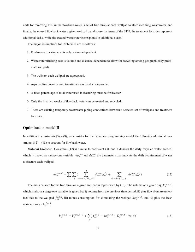
units for removing TSS in the flowback water, a set of frac tanks at each wellpad to store incoming wastewater, and

finally, the unused flowback water a given wellpad can dispose. In terms of the STN, the treatment facilities represent

additional tasks, while the treated wastewater corresponds to additional states.

The major assumptions for Problem II are as follows:

1. Freshwater trucking cost is only volume-dependent.

2. Wastewater trucking cost is volume and distance-dependent to allow for recycling among geographically proxi-

mate wellpads.

3. The wells on each wellpad are aggregated.

4. Arps decline curve is used to estimate gas production profile.

5. A fixed percentage of total water used in fracturing must be freshwater.

6. Only the first two weeks of flowback water can be treated and recycled.

7. There are existing temporary wastewater piping connections between a selected set of wellpads and treatment

facilities.

Optimization model II

In addition to constraints (3) – (9), we consider for the two-stage programming model the following additional con-

straints (12) – (18) to account for flowback water.

Material balances. Constraint (12) is similar to constraint (3), and it denotes the daily recycled water needed,

which is treated as a stage-one variable. dywwsc and dsww

sc are parameters that indicate the daily requirement of water

to fracture each wellpad.

daww,ds =

∑c

∑j

(

d∑d′=d−fDsc+2

dywwsc yd

′jsc +

∑d′=d−fDsc+1

dswwsc yd

′jsc ) (12)

The mass balance for the frac tanks on a given wellpad is represented by (13). The volume on a given day, V ww,ds ,

which is also a a stage-one variable, is given by: i) volume from the previous time period, ii) plus flow from treatment

facilities to the wellpad fwt,dsq , iii) minus consumption for stimulating the wellpad daww,d

s , and iv) plus the fresh

make-up water Dfw,ds .

V ww,ds = V ww,d−1

s +∑q

fwt,dsq − daww,d

s +Dfw,ds ∀s,∀d (13)

12

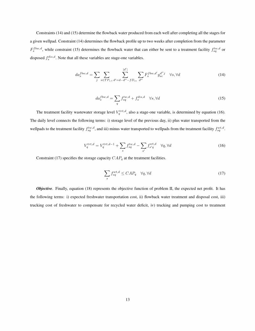
Constraints (14) and (15) determine the flowback water produced from each well after completing all the stages for

a given wellpad. Constraint (14) determines the flowback profile up to two weeks after completion from the parameter

F fbw,ds , while constraint (15) determines the flowback water that can either be sent to a treatment facility f tw,d

sq or

disposed fdis,ds . Note that all these variables are stage-one variables.

dafbw,ds =

∑j

∑s∈TPs,t

|d′|∑d′=d−d′′−fDsc

∑d′′

F fbw,d′

s yd′′j

sc ∀s,∀d (14)

dafbw,ds =

∑q

f tw,dsq + fdis,d

s ∀s,∀d (15)

The treatment facility wastewater storage level V trt,dq , also a stage-one variable, is determined by equation (16).

The daily level connects the following terms: i) storage level of the previous day, ii) plus water transported from the

wellpads to the treatment facility f tw,dsq , and iii) minus water transported to wellpads from the treatment facility fwt,d

sq .

V trt,dq = V trt,d−1

q +∑s

f tw,dsq −

∑s′

fwt,ds′q ∀q,∀d (16)

Constraint (17) specifies the storage capacity CAPq at the treatment facilities.

∑s

fwt,dsq ≤ CAPq ∀q,∀d (17)

Objective. Finally, equation (18) represents the objective function of problem II, the expected net profit. It has

the following terms: i) expected freshwater transportation cost, ii) flowback water treatment and disposal cost, iii)

trucking cost of freshwater to compensate for recycled water deficit, iv) trucking and pumping cost to treatment

13

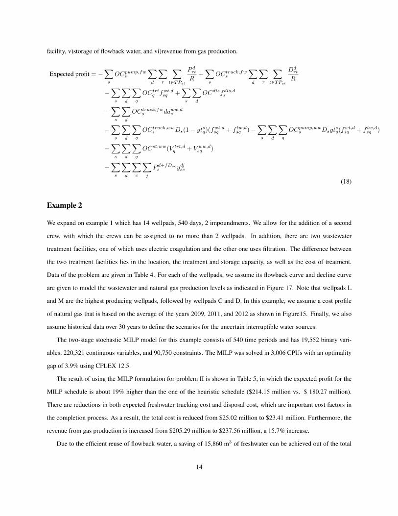
facility, v)storage of flowback water, and vi)revenue from gas production.

Expected profit = −∑s

OCpump,fws

∑d

∑r

∑t∈TPst

P drt

R+

∑s

OCtruck,fws

∑d

∑r

∑t∈TPst

Ddrt

R

−∑s

∑d

∑q

OCtrtq fwt,d

sq +∑s

∑d

OCdisfdis,ds

−∑s

∑d

OCtruck,fws daww,d

s

−∑s

∑d

∑q

OCtruck,wws Ds(1− ytsq)(f

wt,dsq + f tw,d

sq )−∑s

∑d

∑q

OCpump,wws Dsyt

sq(f

wt,dsq + f tw,d

sq )

−∑s

∑d

∑q

OCst,ww(V trt,dq + V ww,d

sq )

+∑s

∑d

∑c

∑j

P d+fDscs ydjsc

(18)

Example 2

We expand on example 1 which has 14 wellpads, 540 days, 2 impoundments. We allow for the addition of a second

crew, with which the crews can be assigned to no more than 2 wellpads. In addition, there are two wastewater

treatment facilities, one of which uses electric coagulation and the other one uses filtration. The difference between

the two treatment facilities lies in the location, the treatment and storage capacity, as well as the cost of treatment.

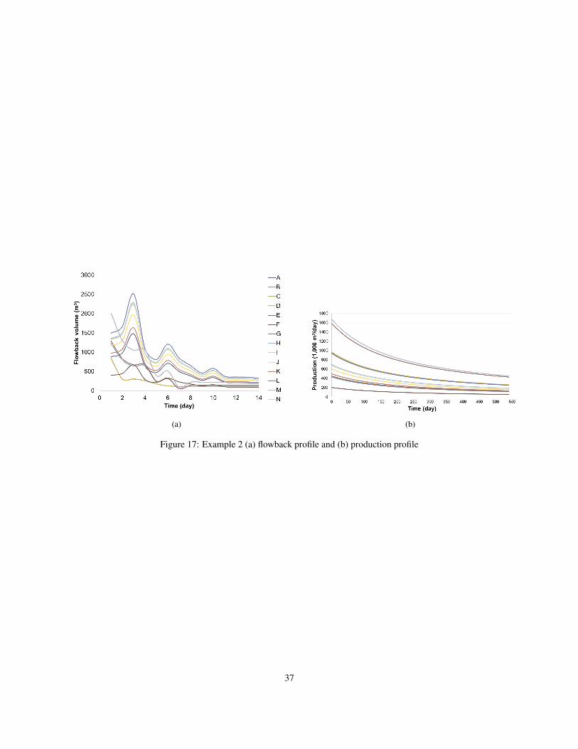
Data of the problem are given in Table 4. For each of the wellpads, we assume its flowback curve and decline curve

are given to model the wastewater and natural gas production levels as indicated in Figure 17. Note that wellpads L

and M are the highest producing wellpads, followed by wellpads C and D. In this example, we assume a cost profile

of natural gas that is based on the average of the years 2009, 2011, and 2012 as shown in Figure15. Finally, we also

assume historical data over 30 years to define the scenarios for the uncertain interruptible water sources.

The two-stage stochastic MILP model for this example consists of 540 time periods and has 19,552 binary vari-

ables, 220,321 continuous variables, and 90,750 constraints. The MILP was solved in 3,006 CPUs with an optimality

gap of 3.9% using CPLEX 12.5.

The result of using the MILP formulation for problem II is shown in Table 5, in which the expected profit for the

MILP schedule is about 19% higher than the one of the heuristic schedule ($214.15 million vs. $ 180.27 million).

There are reductions in both expected freshwater trucking cost and disposal cost, which are important cost factors in

the completion process. As a result, the total cost is reduced from $25.02 million to $23.41 million. Furthermore, the

revenue from gas production is increased from $205.29 million to $237.56 million, a 15.7% increase.

Due to the efficient reuse of flowback water, a saving of 15,860 m3 of freshwater can be achieved out of the total

14

volume required for all 14 wellpads (1.29 million m3). The saving comes from the reduction of freshwater used to

make up for the deficit in recycled water. Since the use of recycled water is assumed to be capped at 15% of the

total volume required to frac the well, the freshwater saving achievable is relatively small. Nonetheless, the saving in

freshwater also implies that less disposal of flowback water is required.

The schedule comparison for fracturing the wellpads is shown in Figure 18. There are three observations worth

noting from the resulting schedule. First, unlike the heuristic schedule, there is no break between the first group of

wellpads, namely, C,D,G,E,N,A,B, and F. This tightness in schedule improves the recycling efficiency of the flowback

water. The second note is that wellpads L and M are stimulated in parallel in the winter when the gas price is

high, leading to higher revenue. Finally, most of the wellpads are completed sooner in the optimized schedule, and

this front-loading scheme allows for a higher overall production level to be achieved within the time horizon under

consideration.

Conclusion

In this work, two-stage programming MILP scheduling formulations have been proposed for shale plays water man-

agement. The goal in Problem I is to balance the trade-off between water acquisition from uninterruptible sources that

are available throughout the year but require more expensive truck transportation, versus acquisition from interruptible

sources that can be transported with pipelines at lower costs but are not available throughout the year. An effective

STN-based model has been developed for this problem. This model has been extended to handle a combination of

disposal options with alternatives for recycling and reuse of flowback water, while accounting for the income from the

sales of natural gas. Using two test cases from operations in the Marcellus Shale development, we have shown the

these models yield cost reduction, revenue enhancement, reduced freshwater consumption, as well as reduced CO2

emissions from transportation. Finally, it should be noted that the models proposed in this work can be coupled with

investment models for shale gas supply chain such as the MINLP model proposed by Cafaro and Grossmann16.

Nomenclature

Indices and sets

c Stages per day fractured scenarios

d, d′, d′′ Time interval

15

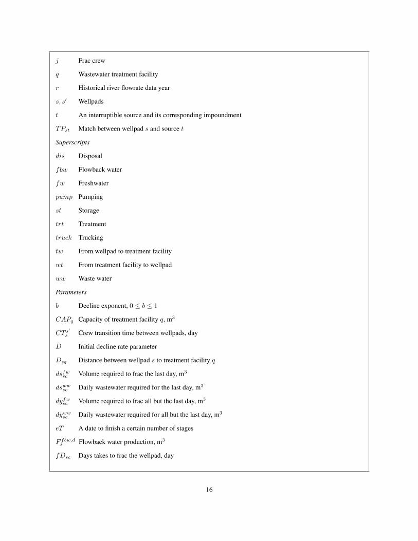
j Frac crew

q Wastewater treatment facility

r Historical river flowrate data year

s, s′ Wellpads

t An interruptible source and its corresponding impoundment

TPst Match between wellpad s and source t

Superscripts

dis Disposal

fbw Flowback water

fw Freshwater

pump Pumping

st Storage

trt Treatment

truck Trucking

tw From wellpad to treatment facility

wt From treatment facility to wellpad

ww Waste water

Parameters

b Decline exponent, 0 ≤ b ≤ 1

CAPq Capacity of treatment facility q, m3

CT s′

s Crew transition time between wellpads, day

D Initial decline rate parameter

Dsq Distance between wellpad s to treatment facility q

dsfwsc Volume required to frac the last day, m3

dswwsc Daily wastewater required for the last day, m3

dyfwsc Volume required to frac all but the last day, m3

dywwsc Daily wastewater required for all but the last day, m3

eT A date to finish a certain number of stages

F fbw,ds Flowback water production, m3

fDsc Days takes to frac the wellpad, day

16

hD Length of frac holiday, day

OCdis Disposal cost, $/m3

OCpump,fws Freshwater pumping cost, $/m3

OCpump,wws Wastewater pumping cost, $/m3/km

OCst,ww Storage cost, $/m3

OCtrtq Treatment facility cost, $/m3

OCtruck,fws Freshwater trucking cost, $/m3

OCtruck,wws Wastewater trucking cost, $/m3/km

P ds Production, $

P0 Initial production, m3

sgTs Total number of stages at each wellpad

T Target number of stages to be completed

ytsq Wastewater piping connection between wellpad s and treatment facility q

Binary variables

ydjsc Defines the beginning of stimulating each wellpad

zd Defines the beginning of a a frac holiday

Continuous variables

Ddrt Deficit in impoundment, m3

dafbw,ds Daily flowback water produced, m3

dafw,ds Freshwater decifit at a wellpad, m3

daww,ds Daily wastewater required, m3

fdis,ds Disposal flowrate, m3

f tw,dsq Flowrate from wellpad s to a treatment facility q, m3

fwt,dsq Flowrate from a treatment facility q to a wellpad s, m3

P drt Pumping rate, m3

tofw,dt Total freshwater required to frac from an impoundment, m3

V drt Volume of the impoundment, m3

V trt,dq Volume of the wastewater in treatment facility, m3

V ww,dsq Volume of the wastewater in frac tank, m3

17

Author Information

Corresponding Author

∗E-mail:grossmann@cmu.edu

Acknowledgments

The authors would like to thank the National Energy Technology Laboratory (NETL) for financial support.

References

1. Stevens P. The ’Shale Gas Revolution’: Developments and Changes tech. rep.Chatham House 2012.

2. Permits Issued and Wells Drilled Maps tech. rep.Pennsylvania Department of Environmental Protection 2013.

3. Marcus O. Gay N. M, Gross S. Water Management in Shale Gas Plays tech. rep.IHS Water White Paper 2012.

4. Mielke E, Anadon L. D, Narayanamurti V. Water Consumption of Energy Resource Extraction, Processing, and

Conversion tech. rep.Energy Technology Innovation Policy research group, Belfer Center for Science and Inter-

national Affairs, Harvard Kennedy School 2010.

5. Holditch S. A. Getting the Gas Out of the Ground Chemical Engineering Progress. 2012.

6. National Water Information System tech. rep.USGS 2013.

7. Birge J. R, Louveaux F. Introduction to Stochastic Programming. Springer 2011.

8. Kondili E, Pantelides C, Sargent R. A general algorithm for short-term scheduling of batch operations –I. MILP

formulation Computers & Chemical Engineering. 1993;17:211 - 227.

9. Shah N, Pantelides C, Sargent R. A general algorithm for short-term scheduling of batch operations – II. Compu-

tational issues Computers & Chemical Engineering. 1993;17:229 - 244.

10. Brooke A, Kendrick D, Meeraus A, Raman R. GAMS: A Users Guide. GAMS Development Corporation 2012.

11. Abdalla C, Drohan J, Rahm B, et al. Waters Journey Through the Shale Gas Drilling and Production Processes in

the Mid-Atlantic Region Penn State Extension. 2011.

18

12. Horner P, Halldorson B, Slutz J. Shale Gas Water Treatment Value Chain - A Review of Technologies, including

Case Studies SPE Annual Technical Conference and Exhibition. 2011.

13. Slutz J, Anderson J, Broderick R, Horner P. Key Shale Gas Water Management Strategies: An Economic Assess-

ment Tool SPE/APPEA International Conference on Health, Safety, and Environment in Oil and Gas Exploration

and Production. 2012.

14. Gaudlip A, Paugh L, Hayes T. Key Shale Gas Water Management Strategies: An Economic Assessment Tool SPE

Shale Gas Production Conference. 2008.

15. Arps J. Analysis of Decline Curves Trans. AIME. 1945.

16. Cafaro D. C, Grossmann I. E. Strategic planning, design, and development of the shale gas supply chain network

AIChE Journal. 2014.

19

List of Figures

1 Wellpad development timeline . . . . . . . . . . . . . . . . . . . . . . . . . . . . . . . . . . . . . . 21

2 Horizontal well hydraulic fracturing stages . . . . . . . . . . . . . . . . . . . . . . . . . . . . . . . . 22

3 Water consumption per unit of energy generation comparison . . . . . . . . . . . . . . . . . . . . . . 23

4 Overall picture of water use in shale gas11 . . . . . . . . . . . . . . . . . . . . . . . . . . . . . . . . 24

5 Water transportation through temporary piping . . . . . . . . . . . . . . . . . . . . . . . . . . . . . . 25

6 River discharge statistics . . . . . . . . . . . . . . . . . . . . . . . . . . . . . . . . . . . . . . . . . 26

7 Problem I superstructure . . . . . . . . . . . . . . . . . . . . . . . . . . . . . . . . . . . . . . . . . 27

8 Daily freshwater requirement for a given wellpad . . . . . . . . . . . . . . . . . . . . . . . . . . . . 28

9 Example 1 fracturing schedule from (a) heuristic method (b) MILP model . . . . . . . . . . . . . . . 29

10 Daily impoundment volume comparison . . . . . . . . . . . . . . . . . . . . . . . . . . . . . . . . . 30

11 Daily truck use comparison . . . . . . . . . . . . . . . . . . . . . . . . . . . . . . . . . . . . . . . . 31

12 Example flowback volume vs. TDS profile13 . . . . . . . . . . . . . . . . . . . . . . . . . . . . . . 32

13 Wellpad impoundment and frac tank aerial view . . . . . . . . . . . . . . . . . . . . . . . . . . . . . 33

14 Well production decline curve . . . . . . . . . . . . . . . . . . . . . . . . . . . . . . . . . . . . . . 34

15 Natural gas price profile averaged over the years 2009, 2010, and 2012 . . . . . . . . . . . . . . . . . 35

16 Problem 2 Superstructure . . . . . . . . . . . . . . . . . . . . . . . . . . . . . . . . . . . . . . . . . 36

17 Example 2 (a) flowback profile and (b) production profile . . . . . . . . . . . . . . . . . . . . . . . . 37

18 Example 2 fracturing schedule from (a) heuristic method (b) MILP model . . . . . . . . . . . . . . . 38

List of Tables

1 Example 1 wellpad data . . . . . . . . . . . . . . . . . . . . . . . . . . . . . . . . . . . . . . . . . . 39

2 Example 1 parameters and cost coefficients . . . . . . . . . . . . . . . . . . . . . . . . . . . . . . . 40

3 Example 1 solution comparison . . . . . . . . . . . . . . . . . . . . . . . . . . . . . . . . . . . . . . 41

4 Example 2 parameters and cost coefficients . . . . . . . . . . . . . . . . . . . . . . . . . . . . . . . 42

5 Example 2 solution comparison . . . . . . . . . . . . . . . . . . . . . . . . . . . . . . . . . . . . . . 43

20

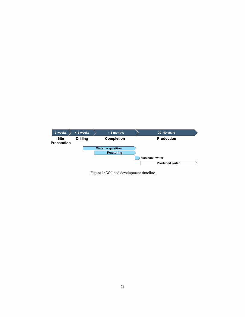
Figure 1: Wellpad development timeline

21

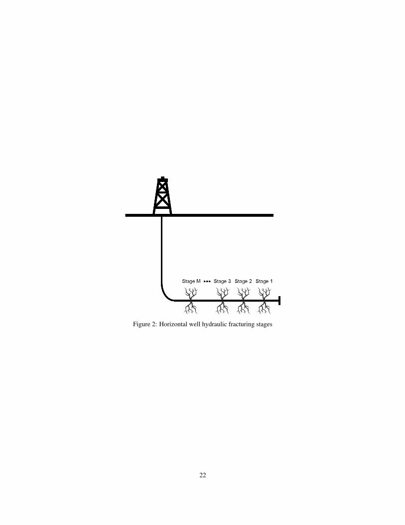
Figure 2: Horizontal well hydraulic fracturing stages

22

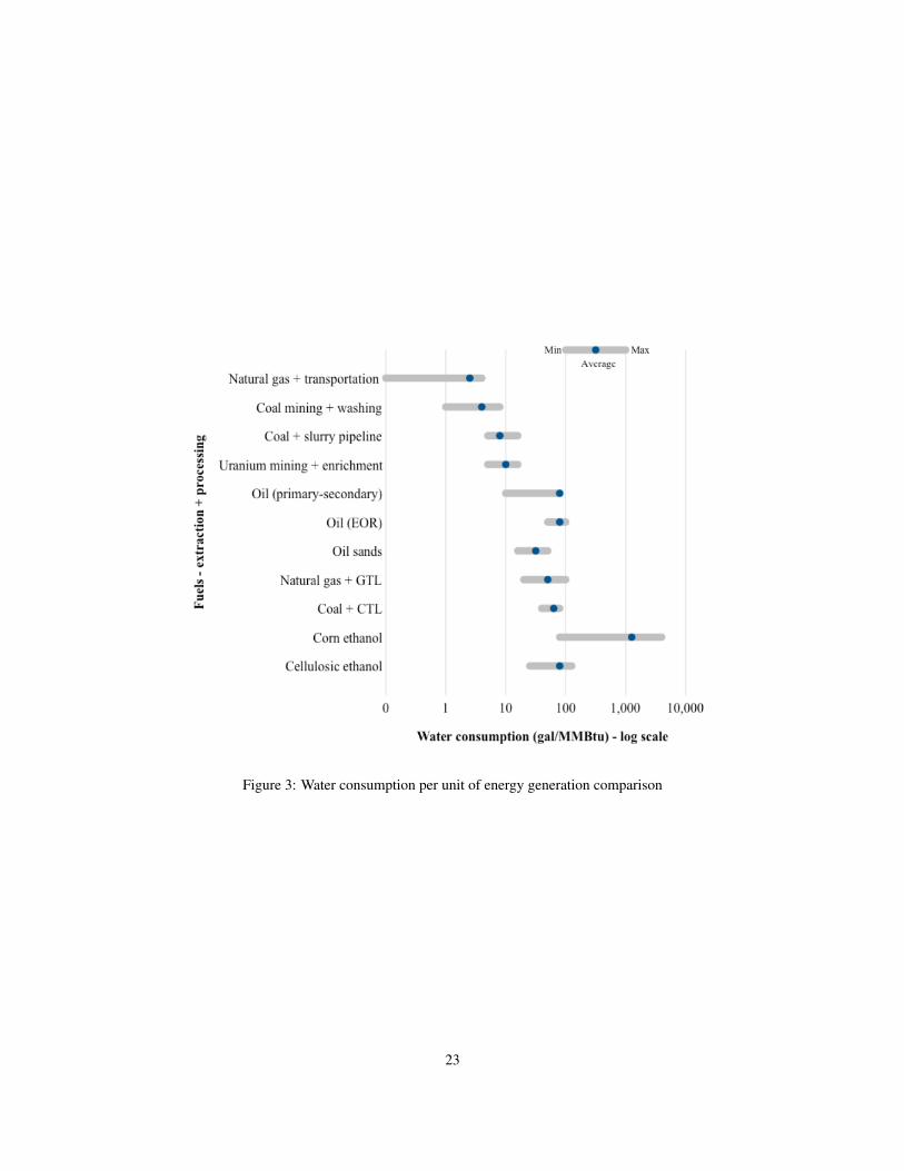
Figure 3: Water consumption per unit of energy generation comparison

23

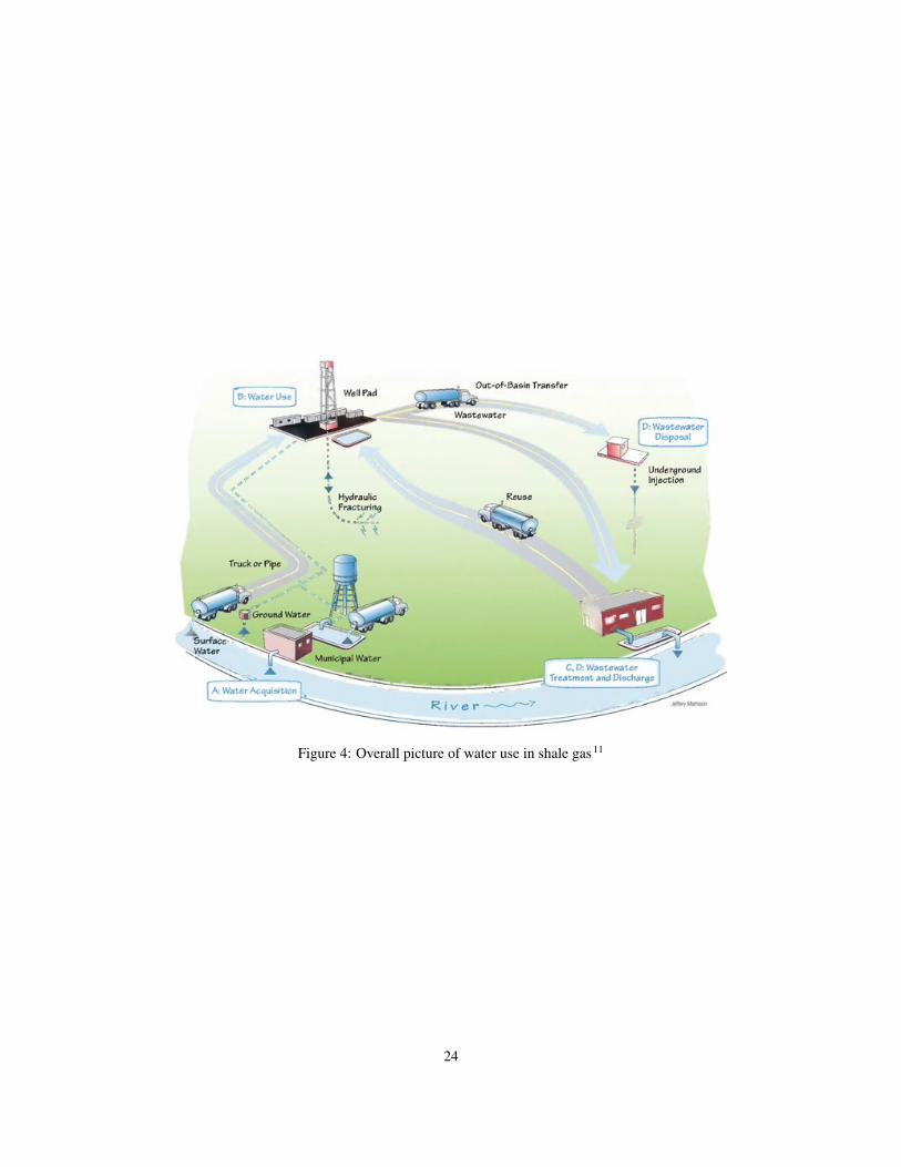
Figure 4: Overall picture of water use in shale gas11

24

Figure 5: Water transportation through temporary piping

25

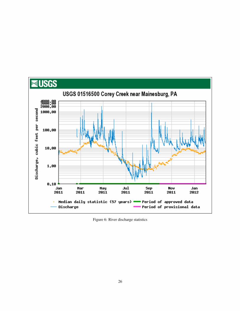
Figure 6: River discharge statistics

26

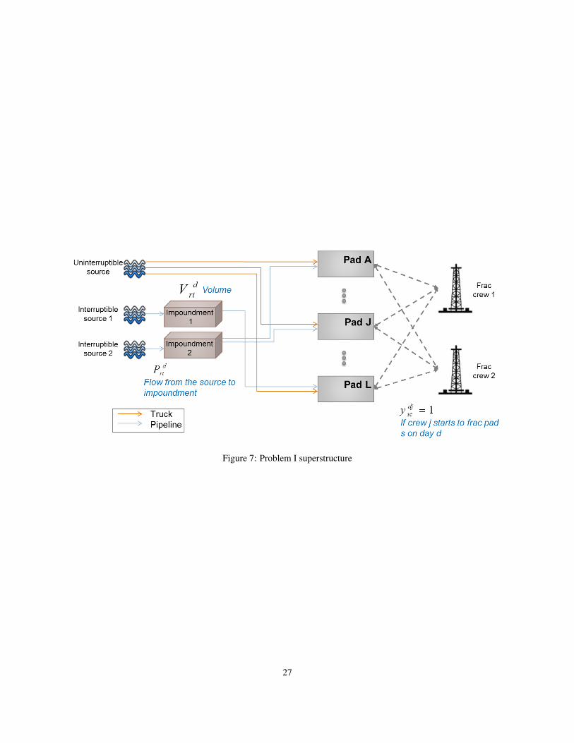
Figure 7: Problem I superstructure

27

Figure 8: Daily freshwater requirement for a given wellpad

28

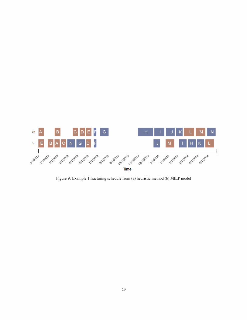
Figure 9: Example 1 fracturing schedule from (a) heuristic method (b) MILP model

29

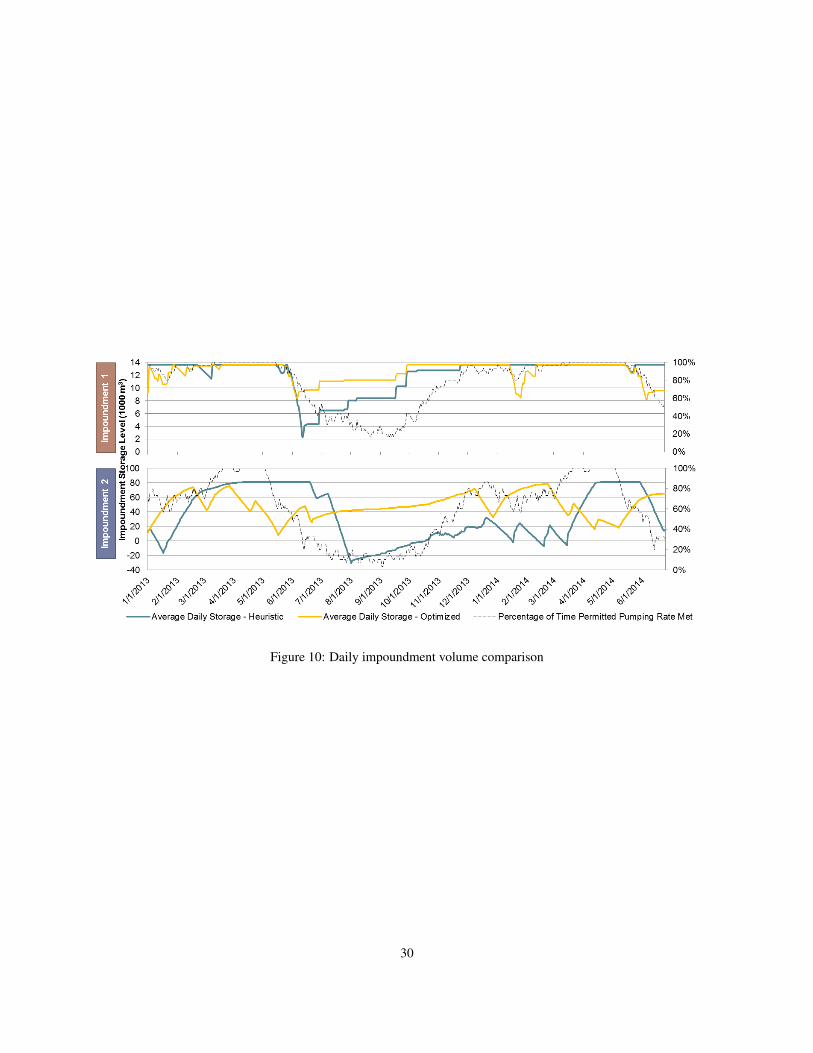
Figure 10: Daily impoundment volume comparison

30

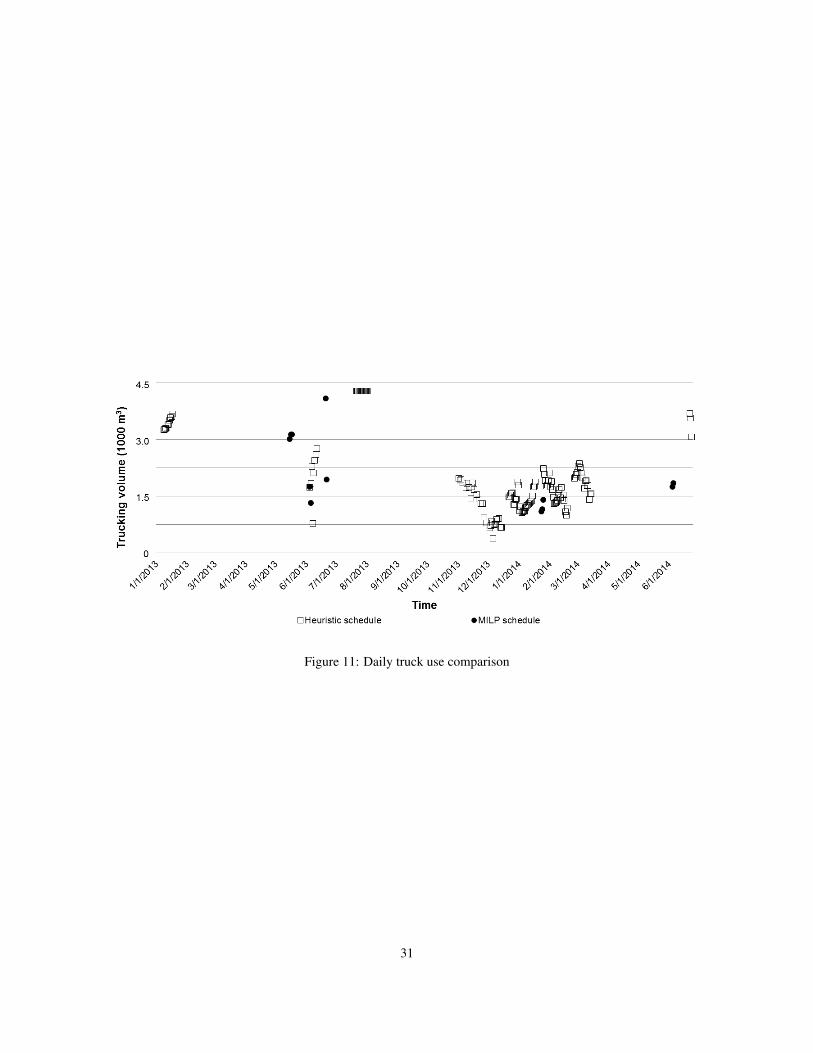
Figure 11: Daily truck use comparison

31

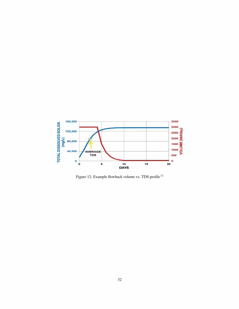
Figure 12: Example flowback volume vs. TDS profile13

32

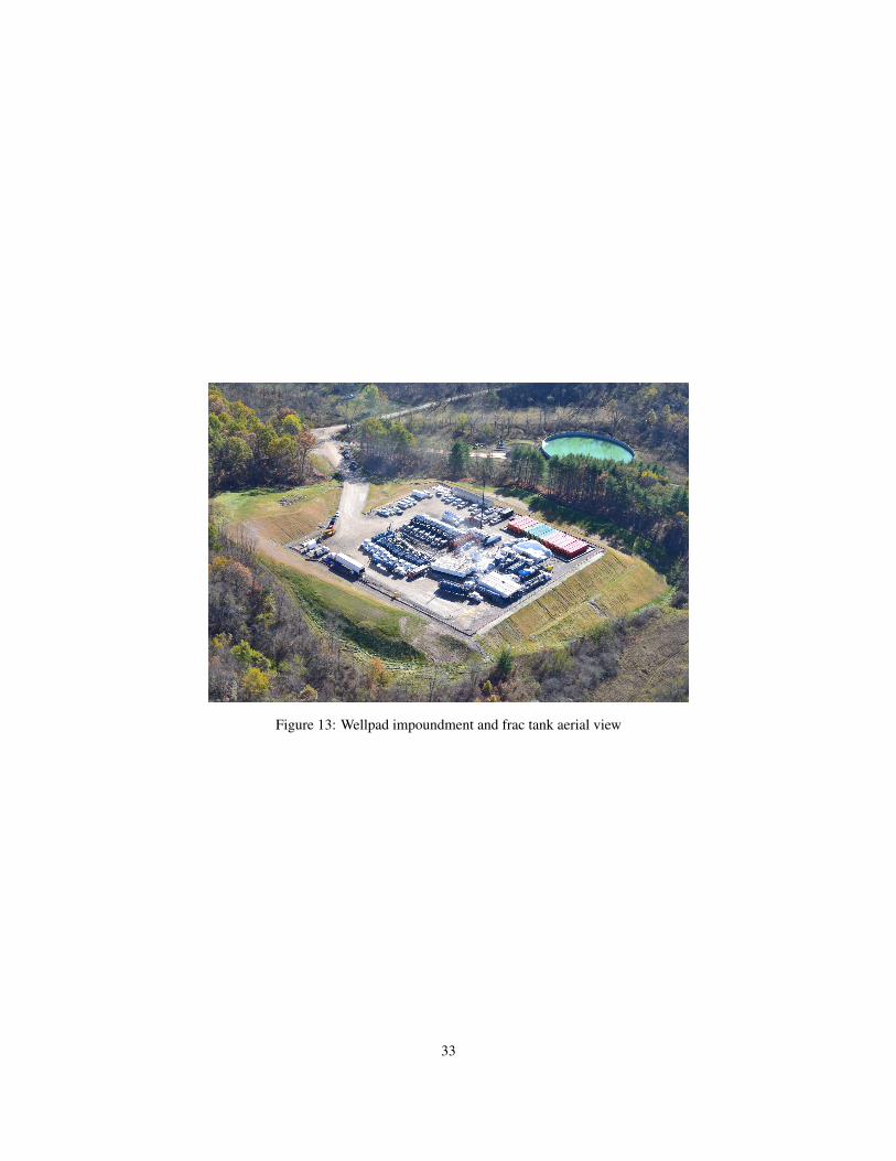
Figure 13: Wellpad impoundment and frac tank aerial view

33

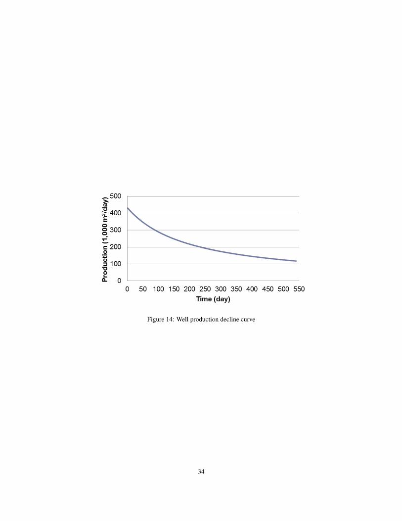
Figure 14: Well production decline curve

34

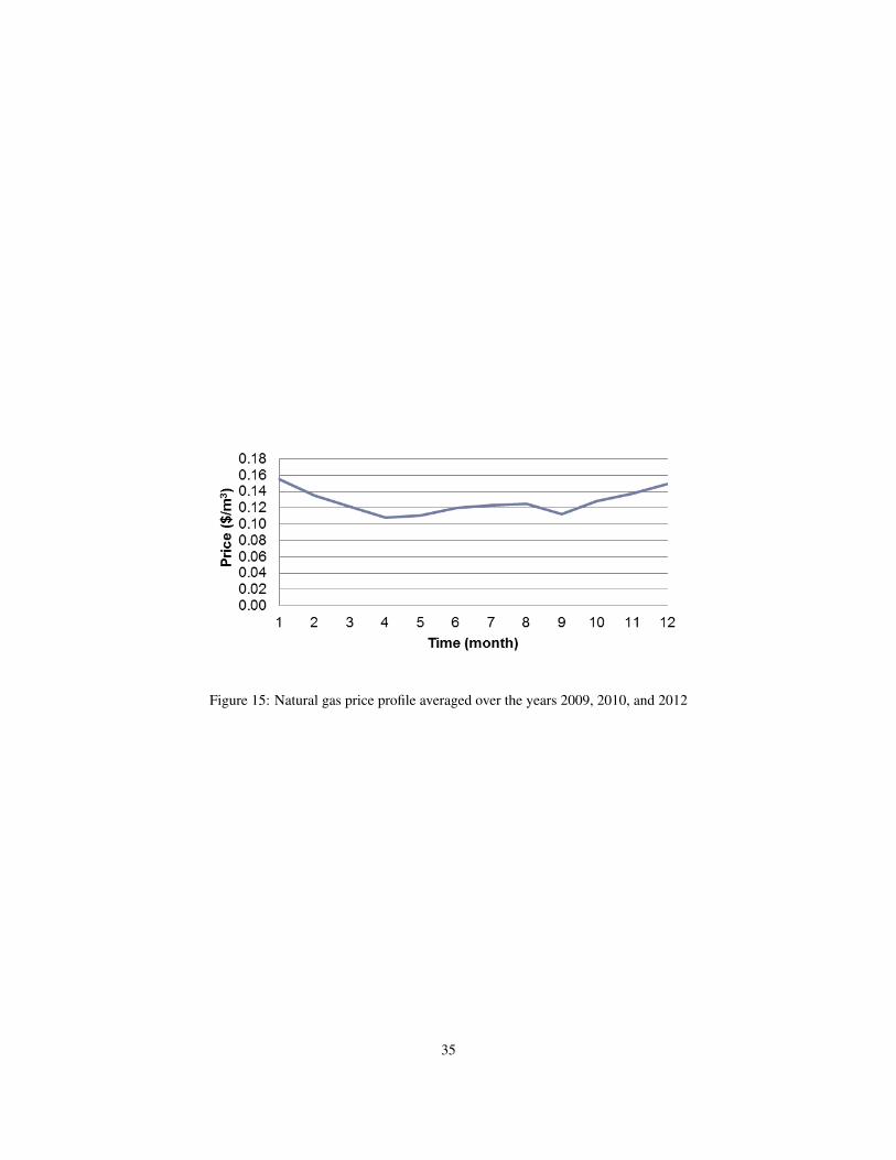
Figure 15: Natural gas price profile averaged over the years 2009, 2010, and 2012

35

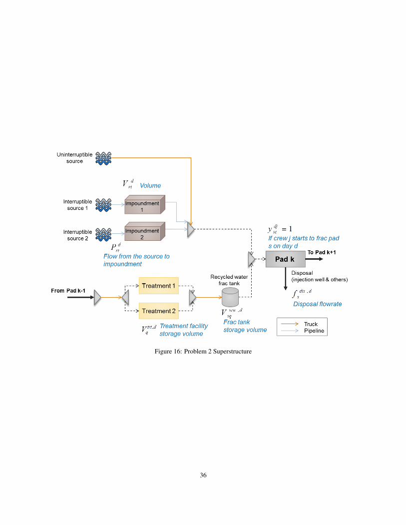
Figure 16: Problem 2 Superstructure

36

(a) (b)

Figure 17: Example 2 (a) flowback profile and (b) production profile

37

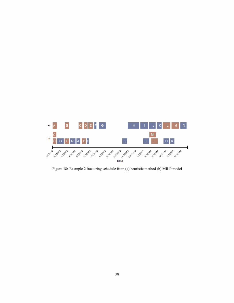
Figure 18: Example 2 fracturing schedule from (a) heuristic method (b) MILP model

38

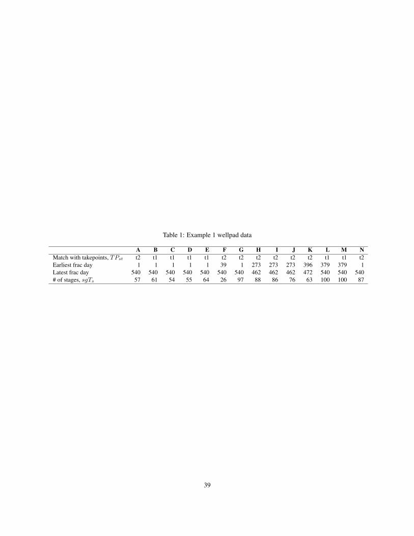
Table 1: Example 1 wellpad data

A B C D E F G H I J K L M NMatch with takepoints, TPst t2 t1 t1 t1 t1 t2 t2 t2 t2 t2 t2 t1 t1 t2Earliest frac day 1 1 1 1 1 39 1 273 273 273 396 379 379 1Latest frac day 540 540 540 540 540 540 540 462 462 462 472 540 540 540# of stages, sgTs 57 61 54 55 64 26 97 88 86 76 63 100 100 87

39

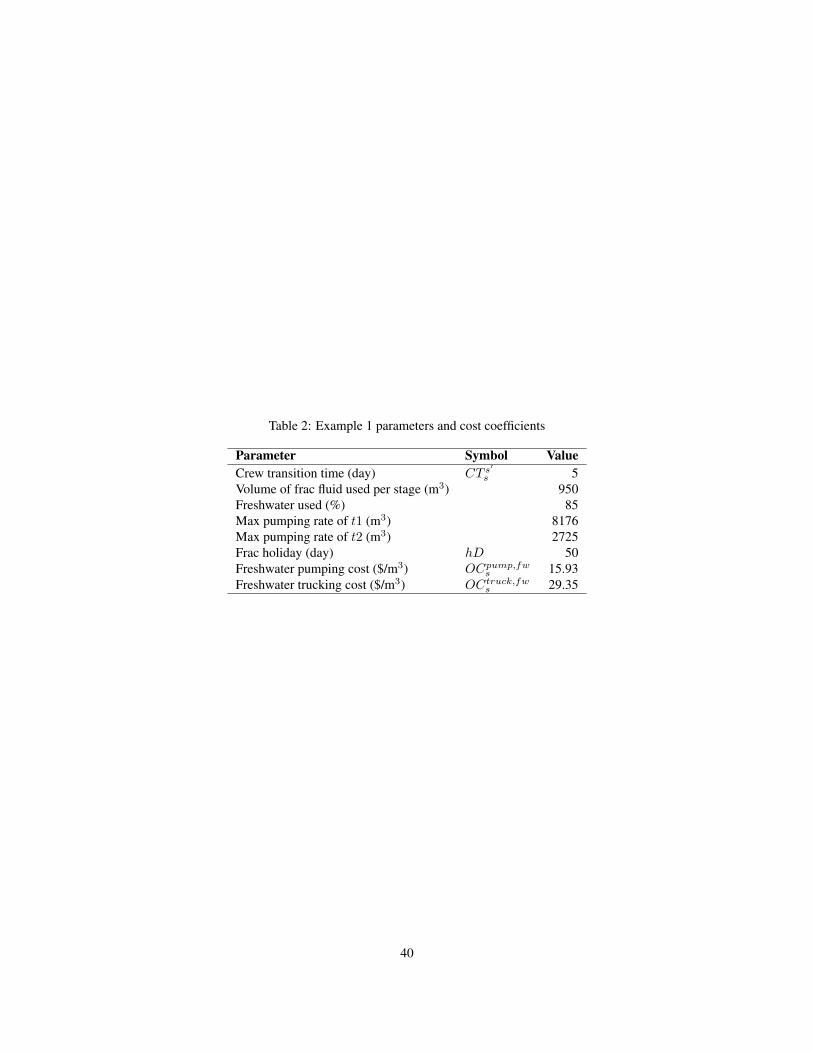
Table 2: Example 1 parameters and cost coefficients

Parameter Symbol ValueCrew transition time (day) CT s′

s 5Volume of frac fluid used per stage (m3) 950Freshwater used (%) 85Max pumping rate of t1 (m3) 8176Max pumping rate of t2 (m3) 2725Frac holiday (day) hD 50Freshwater pumping cost ($/m3) OCpump,fw

s 15.93Freshwater trucking cost ($/m3) OCtruck,fw

s 29.35

40

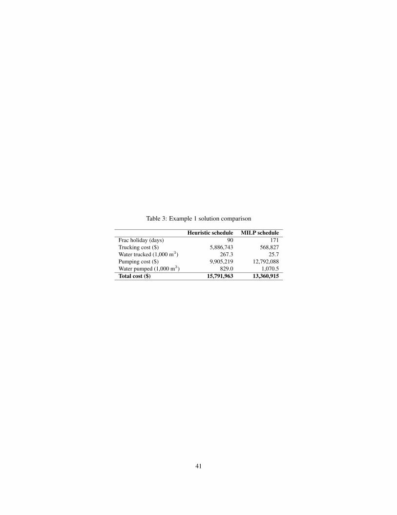
Table 3: Example 1 solution comparison

Heuristic schedule MILP scheduleFrac holiday (days) 90 171Trucking cost ($) 5,886,743 568,827Water trucked (1,000 m3) 267.3 25.7Pumping cost ($) 9,905,219 12,792,088Water pumped (1,000 m3) 829.0 1,070.5Total cost ($) 15,791,963 13,360,915

41

Table 4: Example 2 parameters and cost coefficients

Parameter Symbol ValueCapacity of treatment facility (m3) CAPq q1 = 480 q2 = 1,200Treatment cost ($/m3) OCtrt

q q1 = 25.16 q2 = 12.58Disposal cost ($/m3) OCdis 134.18Storage cost ($/m3/day) OCst,ww 0.59Wastewater pumping cost ($/km/m3) OCpump,ww

s 0.28Wastewater trucking cost ($/km/m3) OCtruck,ww

s 0.15

42

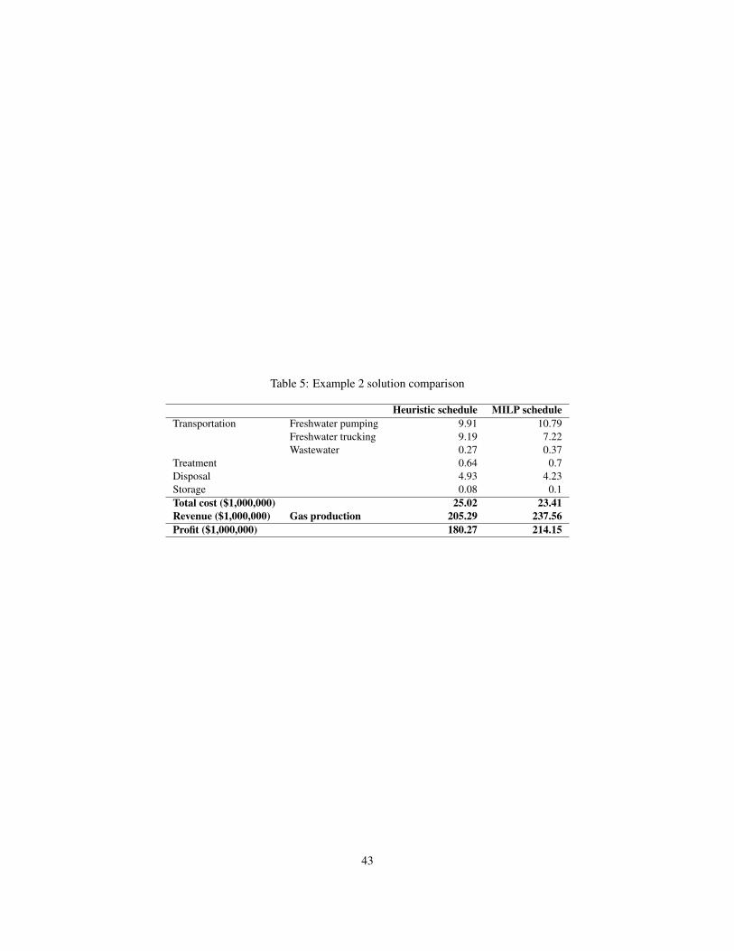
Table 5: Example 2 solution comparison

Heuristic schedule MILP scheduleTransportation Freshwater pumping 9.91 10.79

Freshwater trucking 9.19 7.22Wastewater 0.27 0.37

Treatment 0.64 0.7Disposal 4.93 4.23Storage 0.08 0.1Total cost ($1,000,000) 25.02 23.41Revenue ($1,000,000) Gas production 205.29 237.56Profit ($1,000,000) 180.27 214.15

43