Texas A&M University – Chemical engineering

Optimization of a DL-Methionine Process

Prepared for: Mahmoud M. El-Halwagi, Professors of Sustainable Design Through Process Integration

Prepared by: Team JV Engineering Alejandra EuropaCory AndersonRam SharmaShiv VenkatasettyBharat BaniyaSantiago Nguema

April 30, 2013

Table of ContentsProject Summary.........................................................................................................................................2

Production of DL-Methionine......................................................................................................................4

Pathway...................................................................................................................................................4

Process Description.................................................................................................................................4

Initial Analysis..............................................................................................................................................5

Heat Integration Analysis............................................................................................................................5

Minimum Utility Targeting.......................................................................................................................6

Exchangable Heat Loads..........................................................................................................................7

Network Synthesis.......................................................................................................................................9

Stream Matching.....................................................................................................................................9

Heat Exchanger Sizing............................................................................................................................10

Retrofitting............................................................................................................................................10

Network Summary.................................................................................................................................10

Economic Analysis.....................................................................................................................................11

Utilities Savings......................................................................................................................................11

Heating Utility....................................................................................................................................11

Cooling Utility....................................................................................................................................11

Operating Costs.................................................................................................................................11

Project Cost...........................................................................................................................................11

Return on Investment............................................................................................................................12

10 Year Analysis.....................................................................................................................................12

Conclusions & Recommendations.............................................................................................................15

Additional Recommendations................................................................................................................15

Appendix A: Process Data..........................................................................................................................16

Flowsheet of Process.............................................................................................................................16

Equipment Summary.............................................................................................................................17

Stream Summary...................................................................................................................................18

Appendix B: Gantt Chart............................................................................................................................20

Project SummaryThe JV Engineering Team examined a DL-Methionine production process to identify opportunities for economic improvement through process integration. We recommend that heat integration be pursued; Table 1 summarizes the key changes. A heat exchange network has been synthesized, and will provide savings of $1.04 MM/year. This network contains six heat exchangers and reduces the overall utility usage by 25MMBtu/hr. Three of the exchangers are retrofitted from existing equipment. The total capital investment of the project is $2.316MM. An economic analysis was also performed to determine the profitability of the project. The discounted payback period is 4.2 years at a 15% discounted rate. The return on investment is 33.8% per yer.

Table 1. Results Summary

Summary of ResultsBefore Integration After Integration

Heating Utility 25.8 MMBTU/hr $1.07 MM/yr 0.77 MMBTU/hr $32,000.00/yrCooling Utility 37.93 MMBTU/hr Negligible 12.47 MMBTU/hr Negligible HX Used 5 - 6 $ 2,316,000Total Savings $ 1.04 MM/yr

Problems & Opportunities

The process reviewed for problems and opportunities for process improvement. It was noticed that the process already had significant recycle implemented. Therefore, it was decided that mass integration of the process will not result in significant savings. However, the process uses 4,234 gpm of cooling water

and 60,000 lbhr of steam. After doing some calculations, it was determined that the heating utility is

approximately 49MMBTUhr . It was concluded the operating cost of the process is mainly influenced by

the heating utility, assuming that the cost of cooling water is negligible. It was also decided that the heat

exchangers with less than 1MMBTUhr would be left alone. Therefore, only five heat exchangers were

used for heat integration: two heaters and three coolers. Heat integration was used to minimize the heating and cooling utilities of these exchangers. .These heat exchangers require a heating utility of 25.5 MMBTU/hr and a cooling utility of 37.5 MMBTU/hr.

Heat Integration – Optimization

Heat integration was performed using two methods: using a thermal pinch diagram and an algebraic cascade diagram. Both methods were used to present a visual and an analytical analysis of the process. According to both, the thermal pinch diagram and the cascade diagram, the minimum heating and

cooling utilities are 0.77 MMBTUhr and 12.47

MMBTUhr respectively.

Network Synthesis

The temperature interval diagram was used to synthesize a network of heat exchangers that meets the targets mentioned above. Since the load of H2 exceeds the total sink capacity of the three coolers, H2 was only used to for heat exchange. C2 is the only cooler that needs heating utility. The cooling utility is used to cool H1 and also the residual heat from H2. The proposed network uses a total 6 heat exchangers.

Economic Analysis

The current system of heat exchangers used in the non-integrated process consumes 25.8 MMBtu/hr at a total cost of $1,071,000. After completion of the heat integration project, the new energy usage will be 0.77 MMBtu/hr, for a total cost of $32,000 per year. Using ICARUS, the cost of the integrated heat project is estimated to be about $2,310,150, with an annual operating cost of about $875,000. The ROI of the project, without considering the time-value of money, is 7.35%. When NPV analysis was conducted, a discount factor of 10% and 15% was used to account for the interest and inflation rates during the project period. NPV analysis for a ten-year period showed final cumulative cash flows of $1.61 MM and $2.50 MM at a discount rate of 15% and 10% respectively. This analysis also yielded discounted payback periods of 4.2 years and 3.7 years respectively. At this time, the cumulative cash flow is equal to the original project investment. Although the minimum profitability criteria may vary from corporation to corporation, most profitability factors show this heat integration project to be a sound investment.

Conclusions & Recommendations

Please feel free to contact any members of the team if you have any questions or concerns.

Contact Information

Alejandra Europa: aleuropa92@tamu.edu or 713-373-2131 Cory Anderson: Ram Sharva: Shiv Venkatasetty: Bharat Baniya: Santiago Nguema:

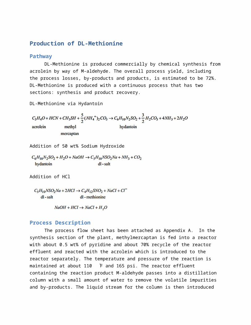
Production of DL-Methionine

PathwayDL-Methionine is produced commercially by chemical synthesis from acrolein by way of M-

aldehyde. The overall process yield, including the process losses, by-products and products, is estimated to be 72%. DL-Methionine is produced with a continuous process that has two sections: synthesis and product recovery.

DL-Methionine via Hydantoin

Addition of 50 wt% Sodium Hydroxide

Addition of HCl

Process DescriptionThe process flow sheet has been attached as Appendix A. In the synthesis section of the plant,

methylmercaptan is fed into a reactor with about 0.5 wt% of pyridine and about 70% recycle of the reactor effluent and reacted with the acrolein which is introduced to the reactor separately. The temperature and pressure of the reaction is maintained at about 110 ͦF and 165 psi. The reactor effluent containing the reaction product M-aldehyde passes into a distillation column with a small amount of water to remove the volatile impurities and by-products. The liquid stream for the column is then introduced to the reactor where the aldehyde is converted to M-hydantoin at 175 ͦF.

After absorption, the hydantoin is hydrolyzed to the DL-salt at in a reactor at 355°F, 150 psi with caustic soda. A vapor stream is pulled from the reactor and cooled. The liquid is then concentrated by evaporating excess water. This water is also cooled and recycled into the process after absorption. The concentrated product is neutralized to DL-methionine and leaves as a slurry to the product recovery section.

In the product recovery section of the plant, the liquid product effluent from the reactor is first distilled to remove an aqueous solution of hydrogen cyanide which is recycled, then concentrated and fed to a crystallizer where crude DL-methionine is precipitated. The crude crystals are collected from the crystallizer slurry effluent in a centrifuge and washed with the mother liquor from the downstream centrifuge.

The crude DL-Methionine crystals are dissolved in water at 195 ͦF, the solution is decolorized, filtered, and fed to a crystallizer. The methionine crystals are collected in a centrifuge, dried, screened and convey to product surge bins for packaging.

Initial AnalysisThe goal of this project is to optimize a plant through process integration. Two types of

implementation were considered: mass targeting and heat integration. First, the overall process was examined to find potential problems and opportunities for process improvement. The process has a well-integrated closed loop water recycle operating in synthesis units. However that recycle loop has a high thermal load that duty that requires preheating and condensation.

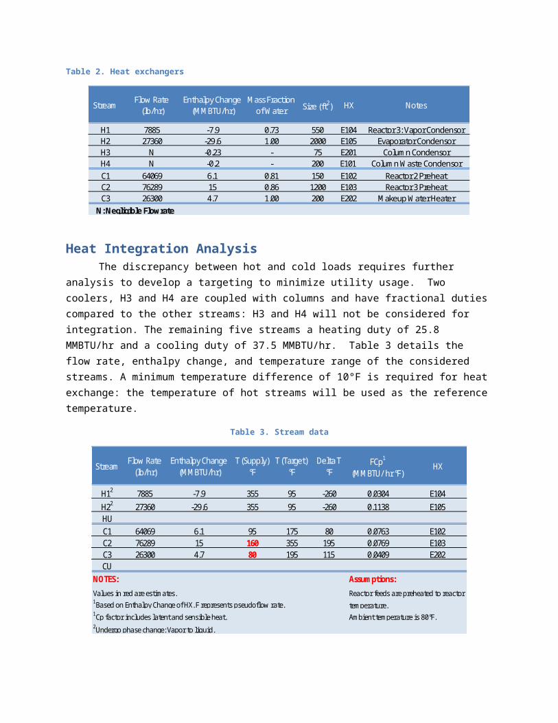
The entire process uses seven heat exchangers: three for heating and four for cooling, Table 2. The streams of these exchangers labeled for easy reference H indicating heat sources, C cold sinks. As built, the process uses external utility to meet these demands. The overall process has an excess of heating of about 12MMBTU/hr.

Table 2. Heat exchangers

StreamFlow Rate

(lb/hr)Enthalpy Change

(MMBTU/hr)Mass Fraction

of Water Size (ft2) HX Notes

H1 7885 -7.9 0.73 550 E104 Reactor 3: Vapor CondensorH2 27360 -29.6 1.00 2000 E105 Evaporator CondensorH3 N -0.23 - 75 E201 Column CondensorH4 N -0.2 - 200 E101 Column Waste CondensorC1 64069 6.1 0.81 150 E102 Reactor 2 PreheatC2 76289 15 0.86 1200 E103 Reactor 3 PreheatC3 26300 4.7 1.00 200 E202 Makeup Water Heater

N: Negligible Flowrate

Heat Integration AnalysisThe discrepancy between hot and cold loads requires further analysis to develop a targeting to

minimize utility usage. Two coolers, H3 and H4 are coupled with columns and have fractional duties compared to the other streams: H3 and H4 will not be considered for integration. The remaining five streams a heating duty of 25.8 MMBTU/hr and a cooling duty of 37.5 MMBTU/hr. Table 3 details the flow rate, enthalpy change, and temperature range of the considered streams. A minimum temperature

difference of 10°F is required for heat exchange: the temperature of hot streams will be used as the reference temperature.

Table 3. Stream data

StreamFlow Rate

(lb/hr)Enthalpy Change

(MMBTU/hr)T (Supply)

°FT (Target)

°FDelta T

°FFCp1

(MMBTU/ hr °F)HX

H12 7885 -7.9 355 95 -260 0.0304 E104H22 27360 -29.6 355 95 -260 0.1138 E105HUC1 64069 6.1 95 175 80 0.0763 E102C2 76289 15 160 355 195 0.0769 E103C3 26300 4.7 80 195 115 0.0409 E202CU

Assumptions:

Reactor feeds are preheated to reactor 1Based on Enthalpy Change of HX. F represents pseudoflow rate. temperature. 1Cp factor includes latent and sensible heat. Ambient temperature is 80°F.

NOTES:

Values in red are estimates.

2Undergo phase change: Vapor to l iquid.

Minimum Utility Targeting From the Table 3, hot and cold composite streams were created corresponding to the overall

heating and cooling loads. When enthalpy of the composite stream is plotted against its temperature, the thermal pinch diagram, Figure 1, estimates the minimum utility usage. The thermal pinch is at 355°F: minimum cooling utility target is 12.42 MMBTU/hr, heating target 0.77 MMBTU/hr.

Figure 1. Thermal pinch diagram

Exchangable Heat LoadsThe overlap in temperature difference with 10° minimum is illustrated in Figure 2. The pinch

point is manifested at 355°F, (345°F for cold). Every overlap in this diagram offers opportunity for heat exchange.

Figure 2. Temperature interval diagram

Using this temperature interval diagram, the tables of exchangeable heat load (TEHLs) for the process hot and cold streams were developed, Tables 4 and 5.

Table 4. TEHL, Hot

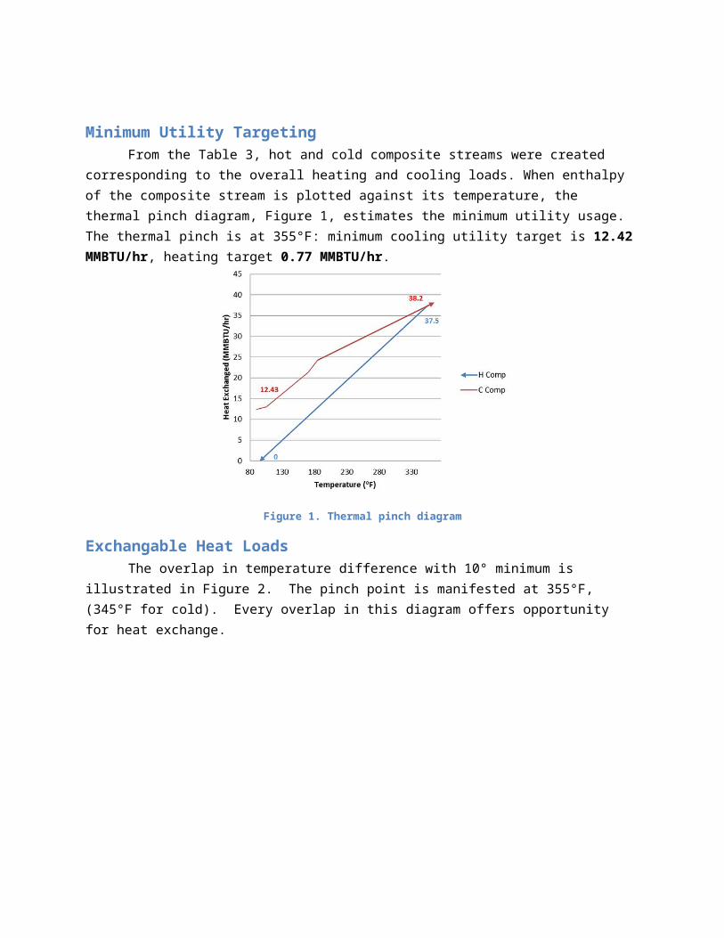
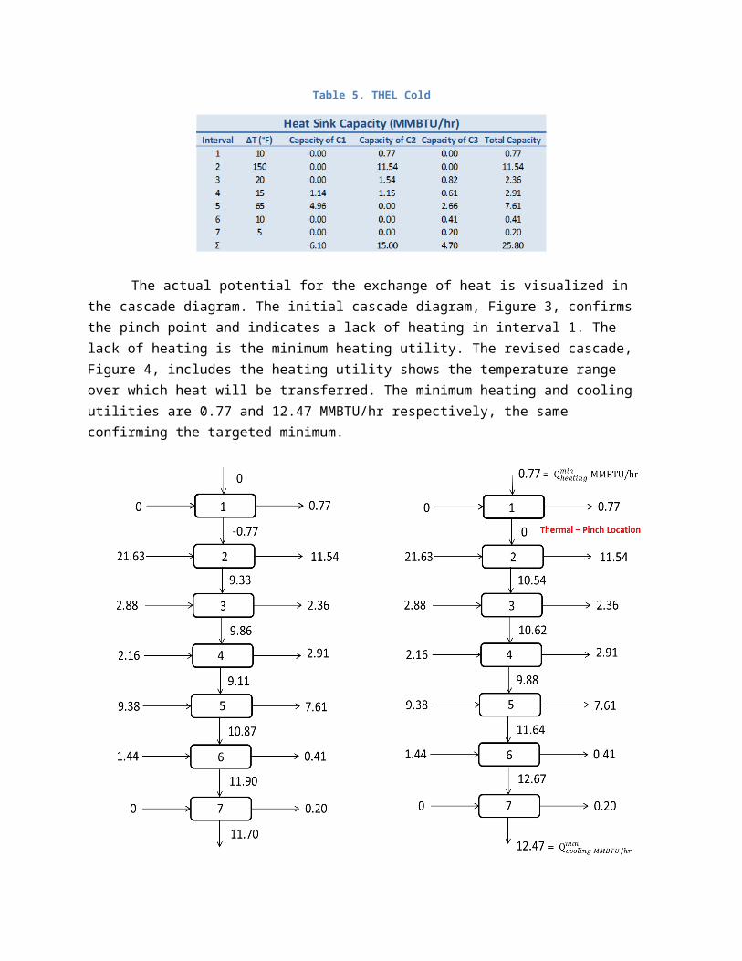
Table 5. THEL Cold

The actual potential for the exchange of heat is visualized in the cascade diagram. The initial cascade diagram, Figure 3, confirms the pinch point and indicates a lack of heating in interval 1. The lack of heating is the minimum heating utility. The revised cascade, Figure 4, includes the heating utility shows the temperature range over which heat will be transferred. The minimum heating and cooling utilities are 0.77 and 12.47 MMBTU/hr respectively, the same confirming the targeted minimum.

Figure 3. Initial Cascade Diagram Figure 4. Revised Cascade Diagram

Network SynthesisThis network will require a total of six heat exchangers. Using the targeted minimums, the

temperature interval diagram was used to synthesize a network of heat exchangers.

Stream Matching

As seen by Figure 2, cooler C2 is the only cold stream with a fraction that cannot be matched

with a hot stream. Therefore, C2 will use the 0.77 MMBTUhr of heating utility calculated in the previous

section. When comparing the heat sources, H2 has a heat load that exceeds the total heat sink capacity of all the cold streams. This allows all the targeted heating demand to be met by a single source.

Figure 7, shows H2 split into three streams of varying flow rates and pairing with the three cold streams. H2 starts as saturated steam at 355 °F (143 psia) and is condensed at 65 psia (298 °F) as saturated liquid for H2C1 and H2C2. H2C3 exits as slightly wet steam. H1 and the residual heat of the H2

fractions, totaling 12.47 MMBTUhr

,are cooled by cooling water.

Figure 5. Stream matching for DL-Methionine. Note: HU and CU refer to heating and cooling utilities.

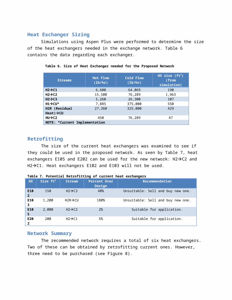
Heat Exchanger SizingSimulations using Aspen Plus were performed to determine the size of the heat exchangers

needed in the exchange network. Table 6 contains the data regarding each exchanger.

Table 6. Size of Heat Exchanger needed for the Proposed Network

Streams Hot Flow (lb/hr) Cold Flow (lb/hr) HX size (ft2)(from simulation)

H2C1 6,600 64,069 190H2C2 15,500 76,289 1,963H2C3 5,260 26,300 107H1CU* 7,885 375,000 550H2R (Residual Heat)CU 27,360 325,000 429HUC2 450 76,289 47NOTE: *Current Implementation

RetrofittingThe size of the current heat exchangers was examined to see if they could be used in the

proposed network. As seen by Table 7, heat exchangers E105 and E202 can be used for the new network: H2C2 and H2C1. Heat exchangers E102 and E103 will not be used.

Table 7. Potential Retrofitting of current heat exchangers HX Size ft2 Stream Percent Over Design Recommendation

E102 150 H2C3 40% Unsuitable: Sell and buy new one.E103 1,200 H2RCU 180% Unsuitable: Sell and buy new one.E105 2,000 H2C2 2% Suitable for application. E202 200 H2C1 5% Suitable for application.

Network SummaryThe recommended network requires a total of six heat exchangers. Two of these can be

obtained by retrofitting current ones. However, three need to be purchased (see Figure 8).

Economic Analysis

Utilities SavingsThe process as specified produces Methionine 90% of the year. The heating utility is provided

by natural gas fired boilers that produce steam at 250 psi. The boilers are 87% efficient. The cooling utility source is assumed to be from an environmental body of water.

Heating UtilityIn order to calculate the cost of heating utility, it was assumed that water was heated using

natural gas. According to the Energy Information Administration (EIA) of the U.S. Department of Energy, the cost of natural gas is $4.58 per MMBTU as of April 24th, 2013. The cost to meet the non-integrated

load, 25.8MMBTUhr , is $1.07MM per year. This proposed network requires $32,000 per year to get

0.77MMBTUhr (see calculations below). The resulting net savings from the heating side is $1.04MM per

year.

Calculations

Heating Utility Before Integration

¿25.8MMBTUhr

× $ 4.581MMBTu

× 24 hr1day

× 365days1 yr

×0.9 stream factor×1.15boiler efficiency=$1,071,000yr

Heating Utility After Integration

¿0.77 MMBTUhr

× $4.581MMBTu

× 24hr1day

× 365days1 yr

×0.9 stream factor ×1.15boiler efficiency=$32,000yr

Figure 6. Heat exchangers required for the recommended network.

Cooling UtilityEnvironmental concerns limit the discharge temperature of the utility back into the reservoir

20°F above the suction temperature. The cooling water reduction is estimated to be near a million pounds per hour. The cooling utility savings are fractional, in the order of 0.01 to 0.001, when compared with the heating.

Operating CostsBy only adding one exchanger, the operating costs of the implementation will not significantly

differ from the operating costs of the current exchangers. No new pumps or additional equipment is added. The largest economic factor comes from the net savings of the heating utilities: $1.04MM.

Project CostAs mentioned earlier, three new heat exchangers are needed. Aspen Process Economic Analyzer

determined the cost of installation of this new network including control and instrument systems. The implementation of these three heat exchangers will require an investment of $2.3MM.

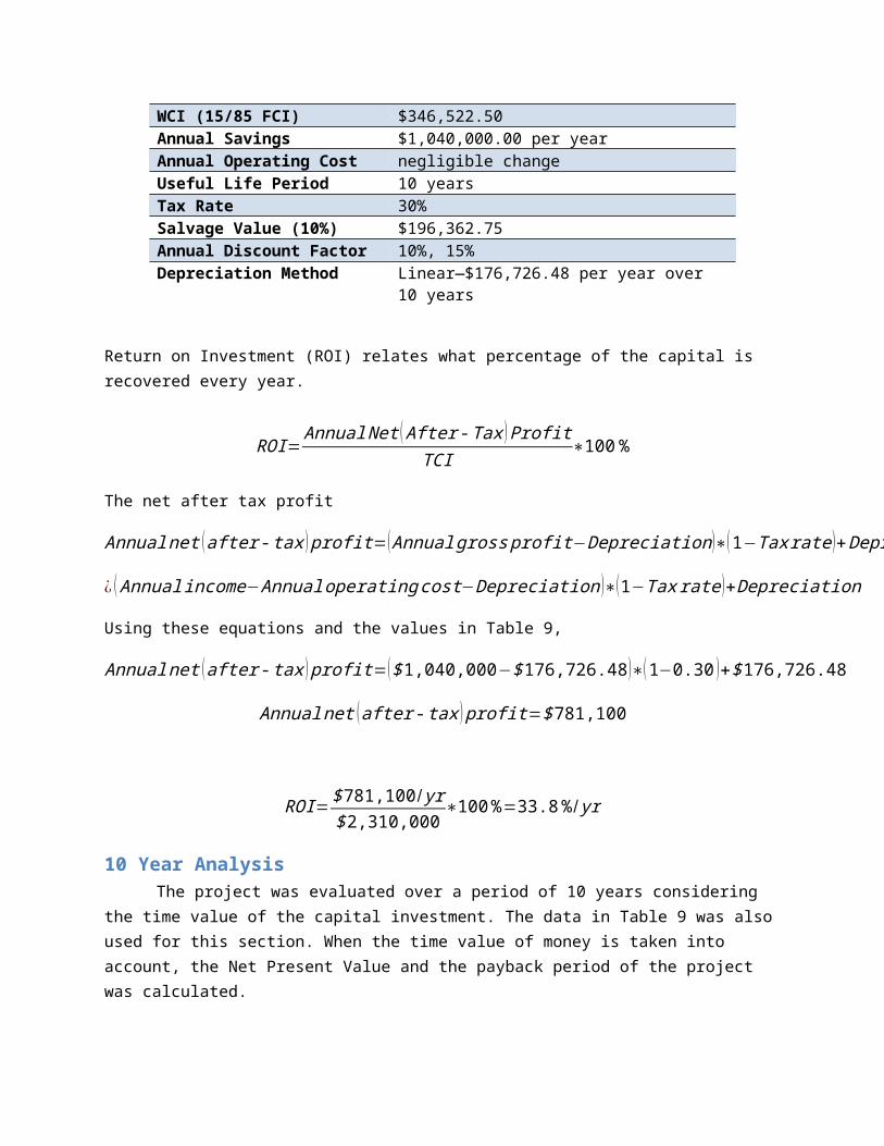
Return on InvestmentTable 8 shows the economic parameters of the recommended network based on the data

discussed above. In order to determine the profitability of the process the return on investment of the process was calculated.

Table 8. Economic Parameters of the Recommended Network

TCI $2,310,150.00WCI (15/85 FCI) $346,522.50Annual Savings $1,040,000.00 per yearAnnual Operating Cost negligible changeUseful Life Period 10 yearsTax Rate 30%Salvage Value (10%) $196,362.75Annual Discount Factor 10%, 15%Depreciation Method Linear—$176,726.48 per year over 10 years

Return on Investment (ROI) relates what percentage of the capital is recovered every year.

ROI= Annual Net (After -Tax )ProfitTCI

∗100%

The net after tax profit

Annualnet (after - tax ) profit=(Annual gross profit−Depreciation )∗(1−Tax rate )+Depreciation

¿ ( Annual income−Annual operatingcost−Depreciation )∗(1−Tax rate )+Depreciation

Using these equations and the values in Table 9,

Annualnet (after - tax ) profit=($1,040,000−$176,726.48 )∗(1−0.30 )+$176,726.48

Annualnet (after - tax ) profit=$781,100

ROI=$ 781,100/ yr$2,310,000

∗100%=33.8% / yr

10 Year AnalysisThe project was evaluated over a period of 10 years considering the time value of the capital

investment. The data in Table 9 was also used for this section. When the time value of money is taken into account, the Net Present Value and the payback period of the project was calculated.

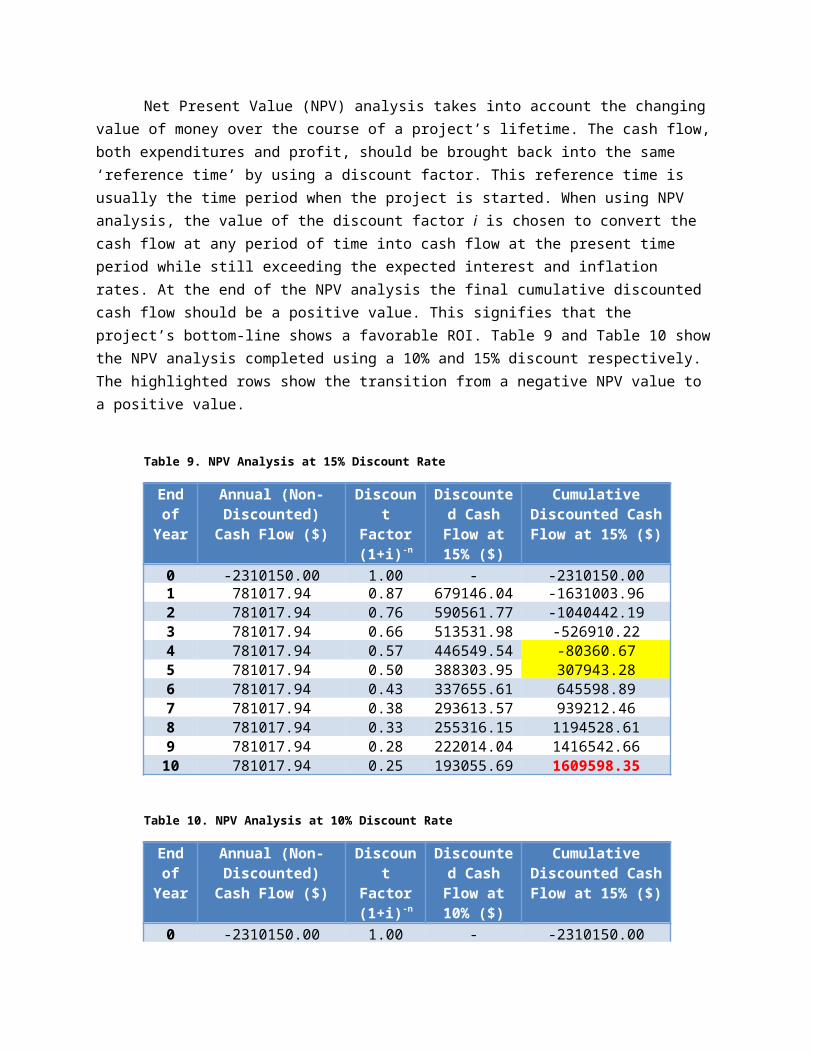
Net Present Value (NPV) analysis takes into account the changing value of money over the course of a project’s lifetime. The cash flow, both expenditures and profit, should be brought back into the same ‘reference time’ by using a discount factor. This reference time is usually the time period when the project is started. When using NPV analysis, the value of the discount factor i is chosen to convert the cash flow at any period of time into cash flow at the present time period while still exceeding the expected interest and inflation rates. At the end of the NPV analysis the final cumulative discounted cash flow should be a positive value. This signifies that the project’s bottom-line shows a favorable ROI. Table 9 and Table 10 show the NPV analysis completed using a 10% and 15% discount respectively. The highlighted rows show the transition from a negative NPV value to a positive value.

Table 9. NPV Analysis at 15% Discount Rate

End of Year

Annual (Non-Discounted) Cash

Flow ($)

Discount Factor (1+i)-n

Discounted Cash Flow at

15% ($)

Cumulative Discounted Cash Flow

at 15% ($)0 -2310150.00 1.00 -2310150.00 -2310150.001 781017.94 0.87 679146.04 -1631003.962 781017.94 0.76 590561.77 -1040442.193 781017.94 0.66 513531.98 -526910.224 781017.94 0.57 446549.54 -80360.675 781017.94 0.50 388303.95 307943.286 781017.94 0.43 337655.61 645598.897 781017.94 0.38 293613.57 939212.468 781017.94 0.33 255316.15 1194528.619 781017.94 0.28 222014.04 1416542.66

10 781017.94 0.25 193055.69 1609598.35

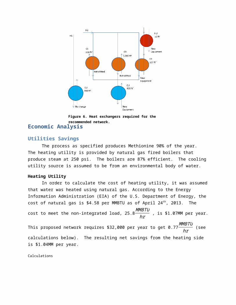
Table 10. NPV Analysis at 10% Discount Rate

End of Year

Annual (Non-Discounted) Cash

Flow ($)

Discount Factor (1+i)-n

Discounted Cash Flow at

10% ($)

Cumulative Discounted Cash Flow

at 15% ($)0 -2310150.00 1.00 -2310150.00 -2310150.001 781017.94 0.91 710016.31 -1600133.692 781017.94 0.83 645469.37 -954664.313 781017.94 0.75 586790.34 -367873.974 781017.94 0.68 533445.76 165571.795 781017.94 0.62 484950.69 650522.486 781017.94 0.56 440864.27 1091386.757 781017.94 0.51 400785.70 1492172.458 781017.94 0.47 364350.63 1856523.089 781017.94 0.42 331227.85 2187750.93

10 781017.94 0.39 301116.23 2488867.16

NPV at the end of ten years with 15% Discount Rate = $1.60MM

NPV at the end of ten years with 10% Discount Rate = $2.50MM

In Figure 8, the cumulative discounted cash flow is shown versus time. At the intersection of each line with the x-axis, the Discounted Payback Period (DPBP) is seen. This is the time at which the discounted project cash flow is equal to the original project investment. It can be seen in Figure 8 that the DPBP is 4.2 years with a 15% rate and 3.7 years with a 10% rate.

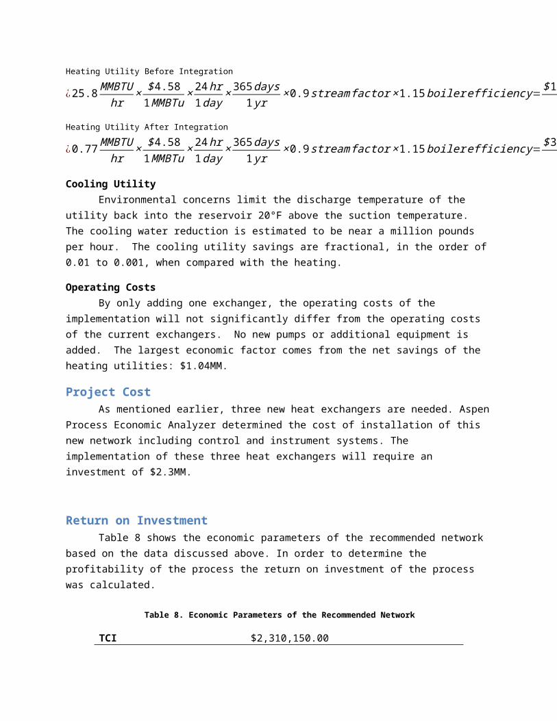
Figure 8. Cumulative Discounted Cash Flow at 10% and 15%

Conclusions & Recommendations

After integrating the heat exchanger network, it was determined that the heating and cooling utilities of the process could be reduced significantly. Originally, the process required 25.8 MMBTU/hr of heating utility, which corresponds to $1.07 MM per year. Through process integration, the heating utility was brought down to 0.77 MMBTU/hr, which corresponds to $32,000.00 per year. This means that by implementing the suggested network, the company will save $1.04 MM in utility cost per year. Throughout the entire analysis, the impact of cooling utility on the overall utility cost was assumed to be negligible. However, it is important to point out that minimizing cooling utility reduces discharge of thermal pollution.

The suggested heat exchange network requires a total of six heat exchangers: three utilizing integrated heat exchange, two cooling utility, and one heating utility. To implement this network, three of the current heat exchangers can be used and three need to be bought. The acquisition of these heat exchangers corresponds to a one time investment of $2.32 MM.

The profitability of the suggested network was analyzed using two models: without and with the time value of money. The return of investment (ROI) of the overall project, without the time value of money, is approximately 7.35% per year. Considering the time value of money, the net present value of the project after ten years will be $ 1.60 MM for a 15% rate and $ 2.50 for a 10% rate. The payback period for the project is 4.2 years for a 15% rate and 3.7 years for a 10% rate. Overall this seems to a profitable project that it is in the interest of the company to implement.

Additional Recommendations

Assuming that the plant will only be running for the estimated 10 years, the company could recover a fraction of the money invested in equipment. With a 10% salvage value, the three heat exchangers bought could be sold for $231,600.00.

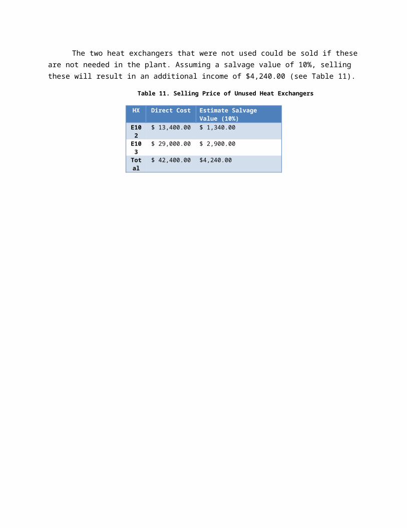
The two heat exchangers that were not used could be sold if these are not needed in the plant. Assuming a salvage value of 10%, selling these will result in an additional income of $4,240.00 (see Table 11).

Table 11. Selling Price of Unused Heat Exchangers

HX Direct Cost Estimate Salvage Value (10%)E102 $ 13,400.00 $ 1,340.00E103 $ 29,000.00 $ 2,900.00Tota

l$ 42,400.00 $4,240.00

Appendix A: Process Data

Flowsheet of Process

Equipment Summary

Stream Summary

Appendix B: Gantt ChartThis Gantt chart summarizes the time management of the group and the progress of the project. The ◊ represents important milestones, while the other symbols indicate tasks. Overall, the tasks were divided among the team. In some occasions, the tasks were performed in small teams. The red and green milestones indicate the start and end of the project. The blue represents the tasks involved with the first facility chosen (Formic Acid). The purple is related to the tasks related to the new/current facility (DL-Methionine).