optimization of an external fuel tank of a...

OPTIMIZATION OF AN EXTERNAL FUEL TANK OF A

SPACE SHUTTLE By

Raghunath Sai Katragadda, Mechanical Graduate Student

Padmaja, Mechanical Graduate Student

Sophia Guntupalli, Aerospace Graduate Student

ME 555-09-01

Winter 2009 Final Report

[email protected]

UNIVERSITY OF MICHIGAN, ANN ARBOR, MICHIGAN

mailto:[email protected]

ABSTRACT

In this project, the design of an external fuel tank of a space shuttle is optimized for minimum

weight and first natural frequency. In this optimization project, the objective is to be attained

while ensuring structural and thermal integrity, aerodynamic drag and volume of the fuel carried.

The optimum design of external fuel tank is an iterative process involving several conflicting

objectives and constraints. Every subsystem has an optimum design satisfying the individual

requirements and the designs are ultimately integrated to determine the overall optimum design.

Within the limitations of the model, the problem is shown to exhibit a modest coupling.

Optimization is viewed not only as a method to determine the best design, but, equally

importantly, as a process through which understanding the system under investigation and

unveiling its intrinsic trade-offs. This study explored the multidisciplinary system design

optimization of the External Fuel Tank of the Space-Transportation-System.

TABLE OF CONTENTS

1. INTRODUCTION

2. LIQUID OXYGEN TANK---Raghunath Sai Katragadda

2.1 Design problem statement

2.2 Nomenclature

2.3 Mathematical model

2.4 Model analysis

2.5 Optimization study

2.6 Parametric study

2.7 Results

3. INTER TANK---Padmaja


3.2 Nomenclature


3.4 Model analysis


3.6 Results

4. LIQUID HYDROGEN TANK---Sophia Guntupalli


4.2 Nomenclature


4.4 Model analysis


4.6 Parametric study

4.7 Results

5. SYSTEM INTEGRATION


5.2 Nomenclature



5.5 Results and Conclusion

6. REFERENCES

7. APPENDIX

1. INTRODUCTION

The Space Shuttle External Fuel Tank (SSEFT) is the largest single element and the only major

non-reusable component of the Shuttle system. The SSEFT is 46.88 meters long, 7.8 meters in

diameter and its empty weight is 29,937 kg. It carries more than 2 million liters of cryogenic

propellants that are fed to the orbiter's three main engines during powered flight.

A design optimization study of the Space Shuttle External Fuel Tank (SSEFT) is performed with

a model which although simplified captures some of the important attributes of the system’s

behavior. The goal of this project is to minimize the weight and the first natural frequency of the

SSEFT by varying its geometric characteristics, while keeping in mind the constraints imposed

on it by the materials chosen and the launching conditions. Gradient based method is applied on

the model to reach optimum points. The endeavor of spaceflight in the United Stated is becoming

increasingly scrutinized in terms of both safety and cost effectiveness. The space agency is

aiming towards maximizing the payload by reducing the system weight. Usage of less material

reduces the cost associated with it. The structural integrity of the system is equally important in

spacecraft voyage. The frequency of vibrations of the system should be as low as possible to

avoid amplitude factors and resonance.

The model is divided into three sub systems, namely,

1. The Liquid Oxygen tank

2. The Intertank

3. The Liquid Hydrogen tank

The rationale behind choosing these subsystems is the fact that the SSFET is composed primarily

of these three components which are welded together. Analyzing individual components,

keeping in mind the influence of one on the other is a good way to proceed, since it will help for

smooth system integration.

The study addresses the following issues:

(1) The simplified model of the external tank,

(2) Single objective optimization using gradient based method of subsystems,

(3) Multi objective optimization using gradient based method of the complete system

The system comprises of seven design variables, all of which are geometric in nature. One of the

variables namely the radius of the cylinder is taken to be the same for all the three subsystems

during system integration. This is considered to be a tradeoff owing to the complexities

associated with structuring the model in ANSYS. The integrated system is governed by six

constraints which are multidisciplinary in nature. The constraints include internal and external

stress constraint, buckling stress constraint, thermal stress constraint, coefficient of aerodynamic

drag constraint, volume of liquid oxygen fuel carried and volume of liquid hydrogen fuel carried.

The material of the system, generally Aluminum Lithium alloy 2090, is taken to be the

parameter. Material properties such as elasticity modulus, Poisson ratio, and thermal

conductivity are implicit parameters as they are included in the Ansys Parametric Design

Language (APDL). The entire system and the subsystems were modeled and analyzed using

ANSYS. The optimization exercise was performed using the optimization tool, ISight, using the

NLPQL algorithm.

Figure 1: Exploded view of SSEFT

2. THE LIQUID OXYGEN Tank

2.1 Design Problem Statement

The liquid oxygen tank is also referred to as the “nose cone” of the system. The nose cone forms

the tip of the external fuel tank. This component is structurally as well as aerodynamically very

crucial to the fuel tank. The liquid oxygen fuel in the tank exerts pressure on the internal walls of

the tank. The external walls of the tank are subjected to aerodynamic pressure which is because

of the aerodynamic force that opposes the movement of the system. The shape of the nose cone

should be aerodynamically very efficient since the drag experienced by the tank is primarily

dependent on the shape of the nose cone. The main objective is to minimize the volume of the

nose cone structure (as the aluminum lithium alloy family has the same density, the objective is

to minimize the volume of material used), accommodating internal stress constraint due to fuel

pressure, external stress due to wind pressure, thermal stress constraint due to difference in the

internal and external temperatures, coefficient of aerodynamic drag constraint and the constraint

involving the volume of liquid oxygen fuel carried. The material used for modeling the structure

is Aluminum Li alloy 2090. The volume of the nose cone is related to the geometry of the

structure. Therefore, the design variables in the problem statement are the geometric dimensions

of the structure.

Design Variables:

The design variables comprise of the geometric dimensions of the nose cone. They are the height

of the cone (H), Radius of the cone (Rcone), Height of the Rim (D) and the thickness of the cone

(tcone).

Parameters:

The explicit parameter is the material of the structure. This parameter actually includes sub-

parameters such as elasticity modulus, Poisson ratio, thermal conductivity, yield strength, etc.

2.2 NOMENCLATURE

H: Height of cone in centimeters

D: Height of the Rim in centimeters

: Radius of the cone in centimeters

: Skin thickness of the cone in centimeters

Fstructallowed : Allowable Structural Stress,190e6

Fthermalallowed : Allowable Thermal Stress, 190e6

: Coefficient of Aerodynamic Drag

: Volume of Liquid Oxygen Fuel, 550

Figure 2: Liquid Oxygen Tank

2.3 MATHEMATICAL MODEL

The objective function of the subsystem is to minimize the volume of the cone which depends on

the geometric design variables of the cone.

x = [H, D, , ]

In order to minimize Volume(x)

As the density is constant the objective modifies to Minimization of Volume of material used.

The volume of material, in terms of design variables is given as

Volume =

The objective function is subjected to the following constraints

Structural Stress Constraint:

The structure need to sustain certain stress levels. The structure is subjected to external wind

pressures and internal fuel pressure. The geometry of the structure should be such that, for a

given material, it used should be able to bear the stress levels. The stresses that are developed in

the structure because of these pressures should not exceed the yield strength of the material

employed in the structure. Therefore a stress constraint is included such that the stresses

developed in the structure should always be less than or equal to the yield strength of the

material.

The stresses developed because of the pressure on the walls are determined using simulation

software ANSYS. The stresses at each node of the mesh should be less than or equal to yield

strength of the material used.

g1: Stresses attained from Simulation - Fstructallowed ≤ 0

Here, the factor of safety has not been considered. Maximum allowable stress can be taken as

the limit which provides some leeway during the optimization process.

Thermal Stress Constraint:

The structure gets exposed to harsh temperatures. The external walls and the internal walls of the

structure experience extreme temperatures. The external walls are exposed to the atmospheric

temperatures and the internal walls are exposed to the fuel temperatures. The difference in the

temperatures builds thermal stresses in the structure. The thermal stresses developed within the

structure should be within the yield strength of the material.

The stresses developed because of the temperature on the walls are determined using ANSYS.

The stresses at each node of the mesh should be less than or equal to the allowable stress of the

material used.

g2: Stresses attained from Simulation - Fthermalallowed ≤ 0

Here, the factor of safety has not been considered. Maximum allowable stress can be taken as

the limit which provides some leeway during the optimization process.

Aerodynamic Constraint

The aerodynamic constraint involves the drag coefficient of the areas concerned with the cone.

The aerodynamic drag coefficient for a regular cone is around 0.5. The relation to express the

coefficient of aerodynamic drag is simplified by substituting the standard density of air, take off

velocity and frictional force of air. The values of these factors are taken from NASA website.

The coefficient of drag is mathematically expressed as follows:

The drag coefficient of the nose cone should be less than or equal to the drag coefficient of a

regular cone to reduce aerodynamic frictional forces.

g3:

Fuel Volume Constraint: The volume of Liquid Oxygen carried in the Nose cone should not be

affected by optimization process of the structure. The internal volume available to store the fuel

should be more than or equal to the volume of the fuel carried.

g4: ≤ 0

The geometric design variables are chosen to be within the limitations recommended by NASA

300≤D≤500

1150≤H ≤1350

350≤ ≤550

0.9≤ ≤3

All the units are in terms of centimeters

Figure 3: Internal and External stresses

Summary

Min Volume =

Subjected to

g1: Stresses attained from Simulation - Fstructallowed ≤ 0


g3:

g4: ≤ 0

300≤D≤500

1150≤H ≤1350

350≤ ≤550

0.9≤ ≤3

2.4 MODEL ANALYSIS

Finite element analysis

The structure is modeled and analyzed in ANSYS. Owing to the huge structure of the nose cone,

axisymmetric model is constructed. This reduces the computation time and cost. Aluminum-Lithium

alloy 2090 is used as the material of the structure. The material properties include elasticity modulus

which is 75 Giga Pascal, Poisson’s ratio of 0.34, thermal conductivity of 88 w/m-k, density of

2.59g/cubic cm. For the structural stress analysis, opposing force due to wind is 29929 Newtons and

the internal fuel pressure is 240875 N/ sq.m. The external temperature of the nose cone is provided as

283 K whereas the internal fuel temperature is around 50 K. An initial starting point is considered

within the constraint region of the geometric variables.

Figure 4: Axisymmetric Model of the Nose Cone

Monotonicity Analysis

The constraints g1 and g2 cannot be studied using monotonicity analysis because of the

nonexistence of the mathematical models for these constraints. The objective function and

constraints g3, g4 involve mathematical relationship.

D H f + + + +

g3 - g4 - - - -

Table 1:Monotoncity analysis with two constraints

The monotonocity analysis involving the objective function and two constraints yield that g3 is

active with respect to . The constraint activity can be precisely estimated because of the

non existence of comprehensive mathematical models.

2.5 OPTIMIZATION STUDY

The subsystem is modeled in ANSYS using APDL. The input files for structural stress analysis

and thermal stress analysis are developed using APDL. The nose come subsystem optimization is

carried out using optimization software (ISight FD3.1) linked with ANSYS. The optimization

model was executed based on a model by Christopher Michael Lawson of MIT. In this approach,

the optimization process requires ANSYS to act as a server for generating input and output files

while ISight runs the variable optimization process. The starting points of the design variables

are randomly chosen within the geometric constraints. The initial runs were performed on

Optimus. But due to the incapability of ANSYS to generate simulations within a desirable time

span, ISight is was used. The gradient-based algorithms i.e. Nonlinear Programming Quadratic

Line Search (NLPQL) is used to obtain results. The Simcode palette and the calculator are used

in the optimization process. The arrangement of the system is as follows:

Figure 5: Optimization model in ISight

Two simcode palettes and two calculators are arranged in parallel for the optimization procedure.

The ANSYS input files and output files are incorporated in the simcode. The calculator includes

mathematical relations of the fuel volume and drag coefficient. The optimization run failed when

performing the experiment for the first few times because of improper mapping of the variables.

Different initial starting points within the constraints have been employed over various runs. At

every instance, the solution was converging to the same values. There existed only one active

constraint with positive lagrangian multiplier of value 0.18D3. The solution is being converged

to the same points for different starting points within the constraints, so it can be concluded as

global optimum. The aerodynamic coefficient of drag constraint is the active constraint. A result

could not be attained when the system was scaled. The runs yielded only infeasible solutions. For

the unscaled model, the KKT conditions are satisfied such that the lagrangian multipliers are

zero for inactive constraints and positive for an active constraint. This constraint activity is

consistent with the monotonic analysis. The volume attained from ANSYS is minimized.

Figure 6: Inputs and Constraints employed in ISight

2.6 PARAMETRIC STUDY

The material of the subsystem incorporates many parameters. During the construction of the

model in ANSYS, material properties such as Young’s Modulus, Poisson Ratio, Thermal

Conductivity, Coefficient of Thermal of Expansion, Density, Thermal Stress, and Yield Stress

are used. The material used during optimization study is Aluminum Lithium alloy 2090. A

change in the material brings about change in all the above mentioned parameters. These

parameters are changed in the APDL code of ANSYS. Different compositions of Aluminum

Lithium alloy material are used for the parametric study. The results attained with materials from

the Aluminum Lithium alloy family yielded similar results with a variation of +/- 10 cubic

centimeters. Substantial difference in the results can be visualized when materials way too

different in characteristics are used.

2.7 RESULTS

In optimizing the subsystem for weight reduction, certain tradeoffs were taken into account.

There is a tradeoff between the volume and stress constraints. As the volume of the material

reduces, the structural and thermal stability of the structure varies. An approximation of the true

geometry of the subsystem is considered. Incorporating the true geometric details led to complex

meshing causing ANSYS to crash. So a simplified version of the structure within the true

dimensional range has been considered. The subsystem is designed in ANSYS using ANSYS

Parametric Design Language (APDL). Geometrical tradeoffs are inevitable because APDL is

highly sensitive towards mesh generation. The main objective in optimizing the subsystem was,

to minimize the volume of a given material used in the structure, at the same time withstanding

structural and thermal stresses, vibrations and providing sufficient volume to carry the requisite

amount of liquid Oxygen. The NLPQL algorithm was used because the problem is a

continuously differentiable optimization problem. It works with both feasible and infeasible

initial design points and has a superior rate of convergence. A total of 21 feasible designs are

identified after undergoing 26 design evaluations. The g3 constraint is the active constraint. A

volume percentage reduction of 69% was attained after running the optimization process.

Realistic analysis can be done by accommodating the complexity of the geometry. The radius of

the cone is the design variable which is in common with the other two sub systems.

Optimization Results

Optimization Technique: NLPQL

Failed Run Objective Value = 1.0E30

Failed Run Penalty Value = 1.0E30

Max Failed Runs = 5

Max Iterations = 10

Min Abs Step Size = 1.0E-4

Rel Step Size = 0.01

Save Technique Log = false

Termination Accuracy = 1.0E-6

Use Central Differences = false

Starting design point:

d = 400 [300.0 < x < 500.0]

h = 1260 [1150.0 < x < 1350.0]

r = 420 [350.0 < x < 550.0]

t = 2 [1.0 < x < 3.0]

Total design evaluations: 26

Number of feasible designs: 21

NLPQL termination reason: LINE SEARCH REQUIRED TOO MANY FUNCTION EVALUATIONS

Optimum design point:

Run # = 7

Objective = 1834050.0

Penalty = 0.0

ObjectiveAndPenalty = 1834050.0

d = 406.0

h = 1326.0

r = 460.0

t = 1.0

cd = 6.04E-5

stress = 2642.6

ther = 738740.0

vf = 5.5824E8

vol = 1834050.0

Calculated constraint values at the optimum:

cd (Upper Bound Constraint) = -0.4999395085066163 (satisfied)

ther (Upper Bound Constraint) = -1161260.0 (satisfied)

stress (Upper Bound Constraint) = -1897357.4 (satisfied)

vf (Lower Bound Constraint) = -8241445.700000048 (satisfied)

3. THE INTERTANK


The Intertank acts as a link between the LH2 and the LO2 tanks of the Space Shuttle. It is

basically a thin walled right circular cylinder and acts as a main load bearing element of the

SSEFT. It transmits the weight of the fuel, the External Tank structural weight and the Orbiter

weight to the Solid Rocket Boosters and Thrust loads from the Solid Rocket Boosters to the

Orbiter. It is also subjected to very high temperature gradients due to the fuel tanks on either

side. First, a simplified geometry is considered to represent the Intertank structure. The

simplicity of the geometry enables us to represent the model with pre defined mathematical

equations to conduct initial studies. The intertank was approximated to a right circular cylinder

of Diameter, D, Length, L and thickness, t. D, L and t are the variables in the optimization

problem. The objective is to minimize the volume of the cylinder by changing these variables.

Since the material we use is constant, we are actually optimizing for minimum weight.

Figure 7: Parts of the Intertank

3.2 NOMENCLATURE

E, Youngs modulus of Aluminum Lithium alloy 2090, Pa

L, Length of the intertank, cm

D, Diameter of intertank, cm

P, Internal Pressure in the intertank, MPa

F, Buckling forces on the Intertank, N

t, Skin thickness of intertank, cm

I, Moment of inertia of a cylinder,

σ, Internal stress, Pa

σy, Max allowable stress of Al-Li alloy

fnat, natural frequency of Aluminum-Li alloy, Hertz

f, Frequency of due to applied loading, hertz

3.3 MATHEMATICAL MODEL:

OBJECTIVE:

minimize f=π(D2-(D-t)2)L

SUBJECT TO:

• g1: An Internal Pressure

Since the geometry is approximated to a cylinder, the hoop stress, σ caused due to the internal

pressure, P is given by the mathematical formula, σ=PD/2t.

This stress must be less than the yield strength of Aluminum7075, σy=96.5MPa

g1: PD/2t < σy

• g2: Buckling stress due to launch forces

Since the geometry is approximated to a cylinder, the buckling stresses, σb caused by the launch

forces, F are given by the the formula, σb=My/I

.

Moment of Inertia, I= [3]

This stress must be less than the yield strength of Aluminum7075, σy=96.5MPa

g2: < σy

• g3: Vibrations at Launch conditions

Since the geometry is approximated to a cylinder, the natural frequency is given by

f= [3]

Moment of inertia, I= [3]

Young’s modulus Aluminum 7075, E=71.7GPa

This frequency must be less than the first natural frequency of aluminum7075, fnat=806Hz

g3: < fnat

• Constraint g1: An internal pressure

Interface forces F are caused at the weld-land between the intertank and the two fuel

tanks.

The average pressure, P caused due to these forces was found to be 833.52e5N per unit

area. This pressure causes hoop stresses inside the intertank. These stresses must be less

than the yield strength of material of Intertank

Figure 8: Internal Pressure

• Constraint g2: Buckling due to the launch forces

The average launch forces acting on the Intertank were found to be F=6200.791e2 N per

unit area from the top and a self equilibrated force from the bottom [2]. Due to these

forces, there can be buckling of the thin walled Intertank. Buckling stresses thus

produced must be less than the yield strength of material of Intertank. Aluminum7075,

σy=96.5MPa

Figure 9: Buckling Forces

• Constraint g3: Vibrations at launch conditions

The natural frequency of the structure depends on the geometry. Since we are changing

the dimensions of the system, it must be kept in mind that the frequency of the system

does not exceed the first natural frequency of Aluminum7075, fnat=806Hz. This avoids

failure due to resonance.

Summary

Minimize f= π(D2-(D-t)2)L

Subject to

g1: PD/2t < σy

g2: < σy

g3: < fnat

Further, due to the manufacturing limitations and space constraints of the launch site, the geometric dimensions were given upper and lower bounds

Geometric Constraints

g4: 400<L<800

g5: 600<D<1000

g6: 0.8<t<1

g7: 0.5< (L/D) <3

3.4 MODEL ANALYSIS

MONOTONICITY ANALYSIS:

Monotonicity analysis was conducted on the above model to determine active and inactive

constraints. The following Monotonicity Table summarizes the analysis.

D T L f + + +

g1 - g2 - g3 -

Table 2: Monotonicity Table

From the monotonicity table, the objective function, f is monotonically increasing in all the

variables. The variables need an upper bound in order to obtain a feasible solution space. On

conducting monotonicity analysis, by MPI, all the constraints are active.

g1 is the stress constraint which is active with respect to the variable, t. It is understood that,

as the thickness decreases, the greater is the stresses produced on the walls of the intertank

g2 is the buckling constraint which is active with respect to the variable, L. The smaller the

length of the intertank, lesser the chances of reaching critical buckling stress.

g3 is the frequency constraint which is active with respect to the variable, D.


The summary model was solved using Excel Solver to obtain initial feasible points. The design

space was sampled at 4 different starting points. All minimized the objective function to

863751.3mm3

S.No f* mm3

Starting Point Optimum Point R=D/2 (mm)

L (mm)

t (mm)

R*=D*/2 (mm)

L* (mm)

t* (mm)

1(random point)

863751.3 2 2 2 357.6304 476.9605 0.806329

2(lower bound)

863751.3 600 400 1 355.729 471.9228 0.819292

3(middle) 863751.3 800 600 1 358.5706 479.444 0.8 Table 3: Optimization Points

The optimum points lie around the same value no matter where we approach it from. A Feasible region can thus be established for the Geometric Constraints.

The lower and upper bounds on the variables were narrowed down using the Excel Solver results

as

300<L<400

800<D<1000

0.7<t<0.9

These bounds also ensure a good L/D ratio.

Now that a rough idea is obtained on the feasible regions, we can model the problem on its actual

geometry. This model has a more complicated geometry since it simulates the existing intertank.

Due to this complication, no mathematical formulae exist to determine stresses and frequencies

produced in the model.

In order to overcome this problem, a Finite Element Model of the intertank was generated in

ANSYS using the ANSYS Parametric Design Language (APDL) in order to run it in Batch

mode. The FEA model was constructed in terms of the variables in the geometry. The model is

then analysed using Finite Elements to obtain the stresses which cannot be otherwise calculated

using simple mathematical equations. The results are written in output files.

The intertank was modeled as a cylinder of length L, thickness, t and radius D. Further, five

stiffener panels of radius H were added at equal distances along the length of the intertank. The

stiffeners suppress Lateral Torsion Deflection of the intertank. Two flanges at the top and bottom

edges also make the intertank more stable.

Figure 10: Actual Geometry of the Intertank

The geometry was then divided into 156 areas and 12 volumes. These volumes were meshed

using the SOLID92 element. The volume mesh generated 23481 nodes. The model’s external

surface was completely constrained so that its outer geometry does not change and influence the

Orbiter’s aerodynamics. The model was then simulated for stress conditions in the Internal

Pressure (g1) and Buckling stress ( g2) constraints.

Figure 11: Meshed Model

Figure 12: Initial Stress and Buckling Analysis

iSIGHT –FD-3.1 optimization software was used to link the FEA analysis using its SIMCODE

palette. The objective function and the modal analysis (g3 constraint) were inputted using the

calculator palette.

Figure 13: Design Gateway Setup

A Gradient Based Algorithm analysis was done, using NLPQL.

A starting point was chosen as, which is close to the Excel Solver’s optimum values.

L=400cm

D=320cm

H=300cm

t=0.7cm

The Results of the Optimization are attached.

3.6 RESULTS AND DISCUSSIONS

• The Optimum Dimensions were found to be

L=434cm

D=370cm

H=336cm

t=0.78cm

• Two constraints were found to be active, namely, the Stress due to Internal Pressure(g1)

and the Buckling Stress(g2). Both of them had Positive Lagrange Multipliers

• The Volume of the Intertank was reduced by 5.4%


Started on Mon Apr 13 17:37:43 EDT 2009




Max Failed Runs = 5

Max Iterations = 10

Min Abs Step Size = 1.0E‐4

Rel Step Size = 0.1


Termination Accuracy = 1.0E‐6



D = 320.0 [300.0 < x < 400.0]

H = 300.0 [300.0 < x < 400.0]

L = 400.0 [400.0 < x < 500.0]

t = 0.7 [0.7 < x < 0.9]

Completed on Mon Apr 13 20:39:08 EDT 2009



NLPQL termination reason: MAXIMUM NUMBER OF ITERATIONS REACHED


Run # = 66

Objective = 835016.590120464

Penalty = 0.0


D = 370.08399746107386

H = 336.3079643620858

L = 434.76903526584186

t = 0.7817971312272031

f = 835016.590120464

freq = 0.36965429106139847

strbuc = 88.197

stress = 95.731

Calculated constraint values at the optimum: (constraint value is a difference between the bound or target and the output parameter value, scaled and weighted)

stress (Lower Bound Constraint) = ‐192.231 (satisfied)

stress (Upper Bound Constraint) = ‐0.7690000000000055 (satisfied)

freq (Lower Bound Constraint) = ‐0.36965429106139847 (satisfied)

freq (Upper Bound Constraint) = ‐607.6303457089386 (satisfied)

strbuc (Lower Bound Constraint) = ‐184.697 (satisfied)

strbuc (Upper Bound Constraint) = ‐8.302999999999997 (satisfied)

4.LIQUID HYDROGEN TANK


The LH2 tank is the bottom portion of the ET. The tank is constructed of four cylindrical barrel

sections, a forward dome, and an aft dome. The barrel sections are joined together by five major

ring frames. These ring frames receive and distribute loads. The forward dome-to-barrel frame

distributes the loads applied through the intertank structure and is also the flange for attaching

the LH2 tank to the intertank. The aft major ring receives orbiter-induced loads from the aft

orbiter support struts and SRB-induced loads from the aft SRB support struts. The remaining

three ring frames distribute orbiter thrust loads and LOX feedline support loads. Loads from the

frames are then distributed through the barrel skin panels. The LH2 tank has a volume of 53,488

cubic feet (1,514.6 m³) at 29.3 psig (3.02 bar absolute) and −423 °F (20.3 K, cryogenic).

The forward and aft domes have the same modified ellipsoidal shape. For the forward dome,

mounting provisions are incorporated for the LH2 vent valve, the LH2 pressurization line fitting,

and the electrical feed-through fitting. The aft dome has a manhole fitting for access to the LH2

feedline screen and a support fitting for the LH2 feedline.

In our project we simplify the structure of the LH2 tank. We consider a cylindrical tank with

hemi spherical domes on both ends. We analyze this modified structure for the same loads which

are present in the actual tank. The main aim is to obtain an optimum design for the given loading

conditions i.e the internal pressure and temperature. We consider stress analysis and vibration

analysis. The optimization is done using ISIGHT which in turn uses ANSYS for the simulation.

The objective is to increase the payload of the tank without compromising on the stability and

strength. We do this by optimizing the weight of the tank. The external fuel tank is not reusable,

so care should be taken such that the material used for the tank is inexpensive and the machining

time is less.

4.2 NOMENCLATURE

M: Mass

R: Radius of the cylinder

H: Height of the cylinder

T: Thickness of the cylinder

σH: Hoop Stress

σc: Critical load

E: Young’s Modulus

I: Moment of Inertia


Objective Function

The objective of the project is to maximize the payload carried by the tank for the same amount

of fuel. This is done by minimizing the weight of the structure. The model is optimized based on

the maximum stress criteria. The design of the structure is changed and the weight is reduced by

keeping the material properties as constant.

For a cylinder with hemispherical ends:

where:

• R is the radius

• L is the middle cylinder length only, and the overall length is L + 2R

• M is mass

• P is the pressure difference from ambient, i.e. the gauge pressure

• ρ is the density of the pressure vessel material

• σ is the maximum working stress that material can tolerate.

Constraints

The constraints can be classified into two types

Physical constraints: These are constraints which define natural laws and engineering

specifications. In this problem the physical constraints are:

Stress analysis: The structural and thermal loads are applied on the model to obtain the

maximum and minimum stress.

Figure 14: Internal Pressure

Figure 14 shows a hollow cylinder, which is subjected to a uniformly distributed internal pressure P.

The figure details an element of material at some radius r, contained within an elemental cylinder.

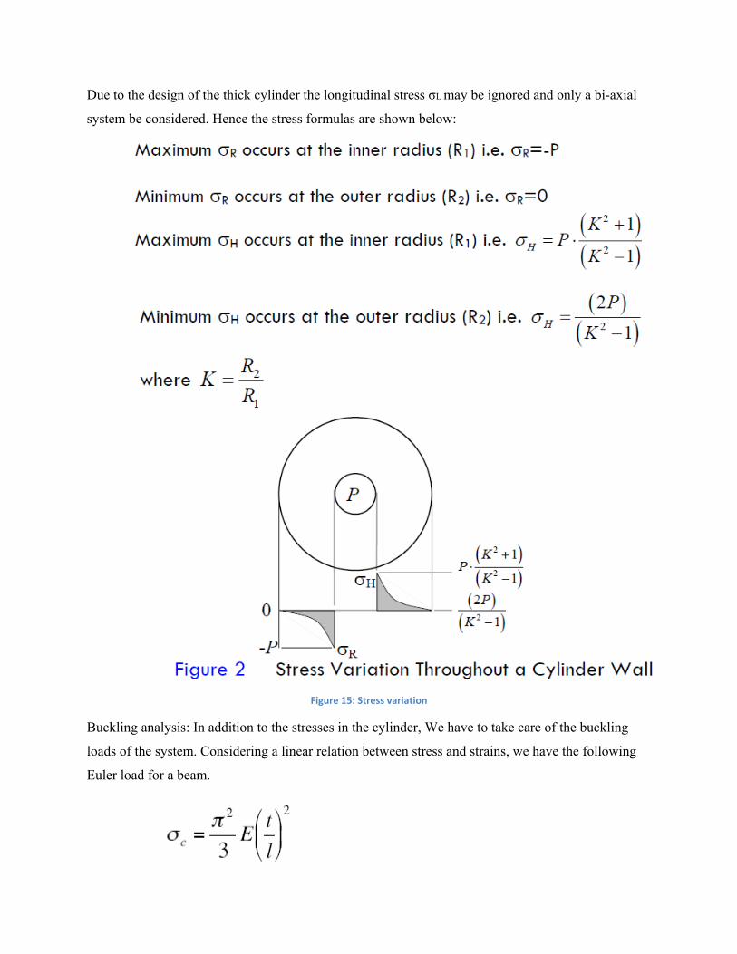
Due to the design of the thick cylinder the longitudinal stress σL may be ignored and only a bi-axial

system be considered. Hence the stress formulas are shown below:

Figure 15: Stress variation

Buckling analysis: In addition to the stresses in the cylinder, We have to take care of the buckling

loads of the system. Considering a linear relation between stress and strains, we have the following

Euler load for a beam.

The buckling load in the cylinder should be less than this critical load.

Modal analysis: Since the cylinder has some vibration will it is under motion, there might be a

possibility of resonance occurring in the cylinder if the frequency of vibration of the cylinder

exceeds its natural frequency. A Free-Free modal analysis is carried out to make sure that the

given model does not exceed the natural vibration of the material.

Freq(cylinder) ≤Freq(material)

Freq(cylinder), f=

Practical constraints: These constraints provide bounds to the variables used. This includes that

all variables are positive and non zero. For a light weight model we arbitrarily assign bounds on

the variables to find the optimized result.:

Diameter: The diameter of the tank can vary between 5 to 10 meters (actual diameter = 8.4m).

Length: The length of the tank can vary between 10 to 40 meters (actual length = 29.5 m)

Thickness: The thickness of the tank should be positive and non zero.

Design variables and Parameters

Design variables are quantities that specify different states of a system by assuming different

values. Parameters are quantities that are given a specific value in any particular model

statement. They are fixed by the application of the model, rather than by the underlying

phenomenon.

The variables for this problem are:

• Radius of the cylinder

• Length of the cylinder

• Thickness of the cylinder

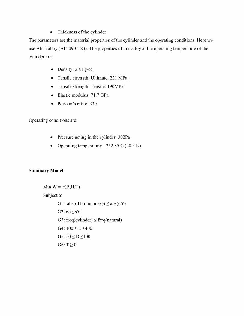
The parameters are the material properties of the cylinder and the operating conditions. Here we

use Al/Ti alloy (Al 2090-T83). The properties of this alloy at the operating temperature of the

cylinder are:

• Density: 2.81 g/cc

• Tensile strength, Ultimate: 221 MPa.

• Tensile strength, Tensile: 190MPa.

• Elastic modulus: 71.7 GPa

• Poisson’s ratio: .330

Operating conditions are:

• Pressure acting in the cylinder: 302Pa

• Operating temperature: -252.85 C (20.3 K)

Summary Model

Min W = f(R,H,T)

Subject to

G1: abs(σH (min, max)) ≤ abs(σY)

G2: σc ≤σY

G3: freq(cylinder) ≤ freq(natural)

G4: 100 ≤ L ≤400

G5: 50 ≤ D ≤100

G6: T ≥ 0

4.4 MODEL ANALYSIS

Using Monotonicity rules we try to understand the boundness and behavior of the function.

D H T

f + + +

g1 + -

g2 - +

g3 - -

Table 4: Monotonicity Table

The monotonicity analysis concludes that the constraint g1 is active with respect to T, g2 is active with

respect to D and g3 is active with respect to H. This is an approximation of the true model as the stresses

are calculated using ANSYS rather than the approximated mathematical relations.


Using the above problem formulation an optimization study is carried out. One constraint is active and it

has a positive lagrangian multiplier. The result is given below.





Max Failed Runs = 30

Max Iterations = 80

Min Abs Step Size = 1.0E-4

Rel Step Size = 0.0010


Termination Accuracy = 1.0E-6



h1 = 147.0 [140.0 < x < 155.0]

h2 = 144.0 [140.0 < x < 155.0]

h3 = 143.0 [140.0 < x < 155.0]

r1 = 40.0 [30.0 < x < 50.0]

r2 = 39.0 [30.0 < x < 50.0]

r3 = 20.0 [0.0 < x < 50.0]



NLPQL termination reason: LINE SEARCH REQUIRED TOO MANY FUNCTION

EVALUATIONS


Run # = 54

Objective = 1229.62101

Penalty = 0.0


h1 = 147.3390518942312

h2 = 144.02302300752893

h3 = 143.04498455423982

r1 = 39.39530717495598

r2 = 38.80942412484222

r3 = 20.27829688424548

mass = 1229.62101

max_stress = 21509.7183

min_stress = 12053.4611

ux_max = 0.107045183

uy_max = -0.0810246568

uz_max = 0.107045183

Calculated constraint values at the optimum:

(constraint value is a difference between the bound or target

and the output parameter value, scaled and weighted)

max_stress (Lower Bound Constraint) = -43609.7183 (satisfied)

max_stress (Upper Bound Constraint) = -590.2816999999995 (satisfied)

min_stress (Lower Bound Constraint) = -34153.4611 (satisfied)

min_stress (Upper Bound Constraint) = -10046.5389 (satisfied)

ux_max (Lower Bound Constraint) = -5.107045183 (satisfied)

ux_max (Upper Bound Constraint) = -4.892954817 (satisfied)

uy_max (Lower Bound Constraint) = -4.9189753432 (satisfied)

uy_max (Upper Bound Constraint) = -5.0810246568 (satisfied)

uz_max (Lower Bound Constraint) = -5.107045183 (satisfied)

uz_max (Upper Bound Constraint) = -4.892954817 (satisfied)

4.6. PARAMETRIC STUDY

Parametric study is done by varying the parameter value and studying the sensitivity of the

model. Here the only parameter used is the material properties.

We consider the following materials for our parametric studies:

• Al 7075

o Modulus of Elasticity : 71.5 Gpa

o Poisson’s ratio : 0.33

o Tensile strength : 96.5 Mpa

o Density : 2.81 g/cc

• Al 7175-T66

o Modulus of Elasticity : 72 Gpa


o Tensile strength : 520 Mpa


• Al 7475 – T61

o Modulus of Elasticity : 70.3 Gpa


o Tensile strength : 490 Mpa


There are no design modifications obtained by slight changes in the material properties.

4.7. Discussion of Results

The optimum values are given by:

h1 = 147.33

h2 = 144.02

h3 = 143.04

r1 = 39.395

r2 = 38.809

r3 = 20.278

mass = 1229.62

All dimensions in centimeters.

5. SYSTEM INTEGRATION


The integration of the three subsystems was modeled in ANSYS. The common variable which is

the radius of the nose cone/radius of the intertank/radius of the liquid hydrogen tank is taken to

be the same for all the three subsytems. Equating all the three radii is important because the

geometry of the structure demands the need to have the same radii for all the sub systems. This

variable is the linking variable between the systems. The entire system is optimized to minimize

the weight of the structure and the first natural frequency. The material of the structure is taken

as Aluminum Lithium alloy which is a parameter. Considering the usage of this material, the

objective function is modified to minimize the volume of the system. The optimization model of

the system is as follows:

Figure 16: System Model

There are three sim code palettes accommodating structural stress constraints, thermal stress

constraints and modal analysis to attain the first natural frequency. The three calculators include

aerodynamic coefficient of drag and the constraints in regard to the volume of fuel carried in the

liquid oxygen tank and the liquid hydrogen tank. The system involves seven design variables and

six constraints.

5.2 NOMENCLATURE

- Coefficient of aerodynamic drag

- Internal volume of liquid oxygen tank, cubic centimeter

- Internal volume of liquid hydrogen tank, cubic centimeter

Cyr- Radius of the cylinder in centimeters

Cyh- Height of the cylinder in centimeters

Cyt- thickness of the cylinder in centimeters

It- intertank thickness in centimeters

Coh- height of the rim in centimeters

Col- length of the cone in centimeters

Cot- thickness of the cone in centimeters


The problem is a multi objective optimization problem where the volume of the system and the

first natural frequency of the system are minimized. These two objectives are calculated within

the ANSYS software. The objectives are subjected to following constraints:

g1: Internal Stresses attained from Simulation - Fstructallowed ≤ 0

g2: External Stresses attained from Simulation - Fstructallowed ≤ 0


g4:

g5: Volume of liquid oxygen carried - ≤ 0

g6: Volume of liquid hydrogen carried - ≤ 0

Coh = 300 [300.0 < x < 500.0] col = 1150 [1150.0 < x < 1350.0] cot = 1 [0.9 < x < 3.0]

cyh = 2800 [2800.0 < x < 3100.0] cyr = 350 [350.0 < x < 550.0] cyt = 1 [0.9 < x < 3.0] it = 1 [0.9 < x < 3.0]


The system is modeled in ANSYS using axisymmetric elements to reduce computation time and

cost. The system is analyzed for structural stresses, thermal stresses and the modal frequency.

The results attained for system integration are different from the results attained from each

subsystem. Individual subsystems were optimized for a single objective. The integrated system is

optimized for multiple objectives. The second objective which is the minimization of the first

natural frequency has a substantial influence over the first objective. It more or less behaves like

an additional constraint. Also the structural and thermal stress constraints where checked over

the entire subsystem. On the system level, the maximum stresses of the entire system are selected

for optimizing rather than the maximum stresses of every sub system. The input files are

included in the appendix. The model of the system in ANSYS using axisymmetric elements is as

follows:

Figure 17: ANSYS Model

Two constraints are shown to be active for the system optimization. The lagrangian multipliers

are positive (0.23D1 and 0.11D1) and satisfy the KKT conditions. The NLPQL algorithm is used

to optimize the model. The optimization runs failed when the model was scaled because of

continuous generation of infeasible points which violated the constraints. The same solution was

reached irrespective of the starting point. Hence, it is a global solution.

5.5 RESULTS and CONCLUSION

Some of the results from system optimization were consistent with those of the sub system

optimization. The variation among other variables is because of the stricter constraint imposed

by the second objective of system optimization. Also the geometry of the sub systems is not

similar to the geometry incorporated in the system. The fasteners in the intertank are removed

and the curved edges of the liquid hydrogen tank are replaced by sharp edges. One design

variable is taken to be common for all the three subsystem and to eliminate complexities some

variables such as the height of the inter tank are taken as constants. All these approximations and

the inclusion of second objective function vary the system results from those of the subsystems.

The model underwent 27 design evaluations and had two feasible designs. The volume of the

material of the system was reduced by 7.2% and the first natural frequency was reduced to 82726

hertz. As a subsystem, the nose cone had a major impact but when included in to the system its

effect is restricted. The project showcased the difficulties in integrating ANSYS with ISight.

Multi Disciplinary optimization problems include more complexity. Multi objective optimization

problems may have the cases where one objective function behaves as a constraint over the other

objective function.


Optimization Technique: NLPQL Failed Run Objective Value = 1.0E30Failed Run Penalty Value = 1.0E30Max Failed Runs = 5 Max Iterations = 10 Min Abs Step Size = 1.0E-4Rel Step Size = 0.0010Save Technique Log = false

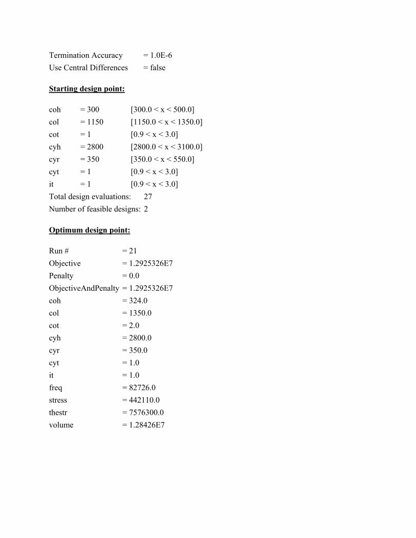
Termination Accuracy = 1.0E-6Use Central Differences = false


coh = 300 [300.0 < x < 500.0] col = 1150 [1150.0 < x < 1350.0] cot = 1 [0.9 < x < 3.0] cyh = 2800 [2800.0 < x < 3100.0] cyr = 350 [350.0 < x < 550.0] cyt = 1 [0.9 < x < 3.0] it = 1 [0.9 < x < 3.0] Total design evaluations: 27 Number of feasible designs: 2


Run # = 21 Objective = 1.2925326E7Penalty = 0.0 ObjectiveAndPenalty = 1.2925326E7coh = 324.0 col = 1350.0 cot = 2.0 cyh = 2800.0 cyr = 350.0 cyt = 1.0 it = 1.0 freq = 82726.0 stress = 442110.0 thestr = 7576300.0 volume = 1.28426E7

6. REFERENCES

1. Heppenheimer, T. A., 2002, Development of the Space Shuttle, 1972-1981, Smithsonian Institution Press, Washington, D.C.

2. Jenkins, Dennis R., 2001, Space Shuttle: The History of the National Space

Transportation System: The First 100 Missions, Specialty Pr Pub & Wholesalers.

3. http://science.ksc.nasa.gov/shuttle/technology/sts-newsref/et.html#et

4. http://www.engineous.com/index.htm

5. Warren C. Young , Richard Budynas “Roark's Formulas for Stress and Strain” McGraw Hill.

6. http://www.uni-bayreuth.de/departments/math/~kschittkowski/nlpql.htm

7. Panos Y. Papalambros and Douglass J. Wilde, “Principles of Optimal Design – Modeling and Computation”, 2nd edition, ISBN 0 521 62727 3, (paperback), Cambridge University Press, 2000

8. R. D. Young, M. P. Nemeth, T. J. Collins, and J. H. Starnes, Jr., NASA Langley Research Center - Hampton, Virginia “Nonlinear Analysis of the Space Shuttle Superlightweight External Fuel Tank”, NASA Technical Paper 3616, December 1996

9. SPACE SHUTTLE EXTERNAL FUEL TANK DESIGN OPTIMIZATION, Massimo

Usan, MIT

10. Multidisciplinary Design Optimization of the Space Shuttle External Tank, Mo-Han Hsieh and Christopher Michael Lawson, MIT

11. insideracingtechnology.com/tech102drag.html

12. Strength of Materials, G.H.Ryder

13. ieeexplore.ieee.org/iel1/20/12212/00560140.pdf?arnumber=560140

14. ANSYS APDLanguage

7. APPENDIX

Input file of System for structural stress and volume

/prep7 cyr=420 cyh= 2950 cyt=2 it=2 coh=400 col= 1260 cot=2 k,1,0,0 k,2,cyr,0 k,3,cyr,cyh k,4,0,cyh k,5,0,cyh-cyt k,6,cyr-cyt,cyh-cyt k,7,cyr-cyt,cyt k,8,0,cyt k,9,cyr,cyh-360 k,10,cyr+it,cyh-360 k,11,cyr+it,cyh+330 k,12,cyr,cyh+330 k,13,0,cyh+80 k,14,cyr,cyh+80 k,15,cyr,cyh+80+coh k,16,0,cyh+80+coh+col k,17,0,cyh+80+coh+col-cot k,18,cyr-cot,cyh+80+coh k,19,cyr-cot,cyh+80+cot k,20,0,cyh+80+cot l,1,2 l,2,3 l,3,4 l,4,5 l,5,6 l,6,7 l,7,8 l,8,1 l,9,10 l,10,11 l,11,12 l,12,9 l,13,14 l,14,15 l,15,16 l,16,17 l,17,18 l,18,19 l,19,20 l,20,13

a,1,2,3,4,5,6,7,8 a,9,10,11,12 a,13,14,15,16,17,18,19,20 et,1,plane42,0,,1 mp,ex,1,75e7 mp,prxy,1,0.34 aesize,2 type,1 mat,1 amesh,all finish /solu antype,0 dl,1,1,all,0 dl,2,1,all,0 dl,3,1,all,0 dl,4,1,all,0 dl,8,1,all,0 dl,9,2,all,0 dl,10,2,all,0 dl,13,3,all,0 dl,14,3,all,0 dl,16,3,all,0 dl,20,3,all,0 sfl,5,pres,2272.63 sfl,6,pres,2272.63 sfl,7,pres,2272.63 sfl,7,pres,(104135780)/(3.14*cyr*cyr) sfl,11,pres,(165354400)/(3.14*it*(2*cyr+it)) sfl,12,pres,416.76e7/(6.28*cyr*cyh) sfl,17,pres,2408.75 sfl,18,pres,2408.75 sfl,19,pres,2408.75 sfl,15,pres,2992900/(9.93*cyr*cyr) solve finish /post1 /OUTPUT,modelstress,dat,, etable,evolume,volu ssum prnsol,s,prin

Input file of System for thermal stress /prep7 cyr=420 cyh= 2950 cyt=2 it=2 coh=400 col= 1260 cot=2 k,1,0,0 k,2,cyr,0 k,3,cyr,cyh k,4,0,cyh k,5,0,cyh-cyt k,6,cyr-cyt,cyh-cyt k,7,cyr-cyt,cyt k,8,0,cyt k,9,cyr,cyh-360 k,10,cyr+it,cyh-360 k,11,cyr+it,cyh+330 k,12,cyr,cyh+330 k,13,0,cyh+80 k,14,cyr,cyh+80 k,15,cyr,cyh+80+coh k,16,0,cyh+80+coh+col k,17,0,cyh+80+coh+col-cot k,18,cyr-cot,cyh+80+coh k,19,cyr-cot,cyh+80+cot k,20,0,cyh+80+cot l,1,2 l,2,3 l,3,4 l,4,5 l,5,6 l,6,7 l,7,8 l,8,1 l,9,10 l,10,11 l,11,12 l,12,9 l,13,14 l,14,15 l,15,16 l,16,17 l,17,18 l,18,19 l,19,20 l,20,13 a,1,2,3,4,5,6,7,8

a,9,10,11,12 a,13,14,15,16,17,18,19,20 et,1,plane77,,,1 mp,kxx,1,8800 aesize,2 type,1 mat,1 amesh,all physics,write,thermal physics,clear etchg,tts mp,ex,1,75e7 mp,prxy,1,0.34 mp,alpx,1,23.6e-7 physics,write,struct physics,clear finish /solu antype,0 physics,read,thermal dl,1,1,temp,283 dl,2,1,temp,283 dl,3,1,temp,270 dl,5,1,temp,20 dl,6,1,temp,20 dl,7,1,temp,20 dl,13,3,temp,270 dl,14,3,temp,283 dl,15,3,temp,283 dl,17,3,temp,50 dl,18,3,temp,50 dl,19,3,temp,50 dl,9,2,temp,283 dl,10,2,temp,283 dl,11,2,temp,283 dl,12,2,temp,270 solve finish /solu physics,read,struct ldread,temp,,,,,,rth dl,all,1,all,0 dl,all,2,all,0 dl,all,3,all,0 solve finish /post1 /OUTPUT,modelthermalstress,dat,,

prnsol,s,prin Input file of system for Modal Analysis /prep7 cyr=420 cyh= 2950 cyt=2 it=2 coh=400 col= 1260 cot=2 k,1,0,0 k,2,cyr,0 k,3,cyr,cyh k,4,0,cyh k,5,0,cyh-cyt k,6,cyr-cyt,cyh-cyt k,7,cyr-cyt,cyt k,8,0,cyt k,9,cyr,cyh-360 k,10,cyr+it,cyh-360 k,11,cyr+it,cyh+330 k,12,cyr,cyh+330 k,13,0,cyh+80 k,14,cyr,cyh+80 k,15,cyr,cyh+80+coh k,16,0,cyh+80+coh+col k,17,0,cyh+80+coh+col-cot k,18,cyr-cot,cyh+80+coh k,19,cyr-cot,cyh+80+cot k,20,0,cyh+80+cot l,1,2 l,2,3 l,3,4 l,4,5 l,5,6 l,6,7 l,7,8 l,8,1 l,9,10 l,10,11 l,11,12 l,12,9 l,13,14 l,14,15 l,15,16 l,16,17 l,17,18 l,18,19 l,19,20 l,20,13

a,1,2,3,4,5,6,7,8 a,9,10,11,12 a,13,14,15,16,17,18,19,20 et,1,plane183,0,,1 mp,ex,1,75e7 mp,prxy,1,0.34 mp,dens,1,2590e-6 aesize,2 type,1 mat,1 amesh,all finish /solu antype,modal modopt,subsp,5 dl,all,1,all,0 dl,all,2,all,0 dl,all,3,all,0 MXPAND,5 solve FINISH /POST1 /OUTPUT,modelfrequency,dat,, set,list set,first pldisp

optimization of an external fuel tank of a...

Documents