Optimization of Automated Float Glass Lines

Byungsoo Na, Shabbir Ahmed∗, George Nemhauser and Joel Sokol

H. Milton Stewart School of Industrial and Systems Engineering,

Georgia Institute of Technology,

765 Ferst Drive, Atlanta, GA 30332

{byungsoo.na, sahmed, gnemhaus, jsokol}@isye.gatech.edu

Statement of Scope and Purpose

Flat glass is approximately a $20 billion/year industry worldwide, with almost all flat glass products being

manufactured on float glass lines. New technologies are allowing float glass manufacturers to increase the level

of automation in their plants, but the question of how to effectively use the automation has given rise to a new

and difficult class of optimization problems not yet studied in the literature. These optimization problems

combine aspects of traditional cutting problems and traditional scheduling and sequencing problems, the

hybrid of which has not previously been modeled, let alone studied or solved. In this paper, we define and

model the problem, and provide heuristic solution methods that produce manufacturing yields greater than

99%. These high-yield solutions can save millions of dollars, so our methods are currently being implemented

at a major float glass manufacturer.

Abstract

In automated float glass manufacturing, a continuous ribbon of glass is cut according to customer orders

and then offloaded using robots. We consider the problem of laying out and sequencing the orders on the

ribbon so as to minimize waste. The problem combines characteristics of cutting, packing, and sequencing

problems. Given the size and the complexity of the problem, we propose a two-phase heuristic approach

where the layout and sequencing aspects of the problem are addressed independently. On a set of real-world

and random instances, our approach achieves schedules with over 99% yield (ratio of glass input and output).

This is a significant improvement for the manufacturer where this work has been implemented.

Key words: Float Line, Glass, Automation, Cutting, Scheduling, Heuristics

∗Corresponding author: Shabbir Ahmed (Fax)1-404-894-2301, sahmed@isye.gatech.edu

1

1 Introduction

Flat glass manufacturing is a continuous process whereby a ribbon of molten glass is produced in a furnace

and then cooled on a bath of molten tin to ensure flatness. The continuous glass ribbon is then carried

on rollers through an annealing lehr, machine-cut according to customer size requirements, and offloaded

for distribution. The equipment in this process, beginning with the furnace and ending with the offloading

equipment, constitutes a float line (see Figure 1).

Assuming that any glass cut could easily be offloaded, the problem of fitting all of the customers’ orders into

the smallest-possible piece of ribbon is very similar to traditional 2-dimensional cutting problems. In this

case, the only way glass is wasted (other than breakage) is in the process of laying out orders on the ribbon.

This wasted glass, or scrap, is known as layout scrap.

This paper considers a float line in a glass plant that has recently fully automated their previously-manual

offloading process. There are clear safety and cost advantages to performing offloading with robots rather

than humans, but the automation is more restricted in the amount of glass it can offload per unit time. As

a result, some additional glass might be wasted if it is cut but cannot be picked up before it gets to the end

of the conveyor. This additional scrap is known as cycle time scrap because it is caused by the cycle time

(minimum time between pickups) of the picking robots. Of course, cycle time scrap could be eliminated by

purchasing more automated equipment, but each robot costs millions of dollars. It is preferable to optimize

the sequence and layout of the glass being cut so that the total amount lost to cycle time scrap and layout

scrap is small.

Although the literature addresses individual aspects of the float glass problem mentioned above, we are

unaware of any model in the literature that deals with the full complexity of the problem. The float glass

problem resembles a guillotine version of the two-dimensional cutting-stock problem (2D CSP) studied by

Gilmore and Gomory [2, 3]. However, the 2D CSP addresses only layout scrap. The float glass problem has

the added complexity of cycle time scrap caused by the relation between the cutting and offloading operations.

Another related problem is two-stage hybrid flow shop (HFS) scheduling with no intermediate storage and

identical parallel machines in the second stage. See Linn and Zhang [6] for general HFS scheduling, and

see Gupta and Tunc [4] for the HFS with parallel machines at the second stage. Also, see Pinedo [8] for

the flow shop with limited intermediate storage. The cutting and offloading operations in the float glass

problem make up the two stages of a flow shop, and minimizing cycle time scrap is equivalent to scheduling

to minimize processing time. However HFS scheduling does not address layout scrap. Dash et al. [1] studied

2

the problem of producing rectangular plates for a steel company to minimize scrap, but do not consider the

sequencing issue. Thus, none of these earlier works adequately captures the full complexity of the float glass

problem.

In [7], we show that the float glass problem is NP-hard in general, and study special cases that can be solved

in polynomial time. We also introduce a mixed-integer programming (MIP) formulation for it. However,

because of the MIP’s size and difficulty, a state-of-the art commercial solver such as CPLEX 11 is unable to

find good solutions within a reasonable amount of time. Therefore, we present a heuristic solution approach

to solving the float glass problem. We will empirically show that the proposed heuristic solution approach

produces nearly-optimal solutions for a collection of randomly generated and real-world test problems.

In Section 2, we introduce the relevant characteristics of a float line, and describe the sequencing and layout

optimization problem. In Section 3, we present heuristic algorithms to solve the problem. Computational

results are provided in Section 4.

2 Problem Description

2.1 Basic Terminology

Our problem concerns processing a given set of customer orders (usually about 60) over a 24 hour working

shift. Each customer order consists of a specified number of identical pieces of glass (plates) of specified

dimension (length × width × thickness). For example, a customer might order 200 plates with dimensions

20 inches by 40 inches by 1 inch. Because it is difficult and costly to change the thickness of the ribbon,

each production shift is typically composed of orders of the same thickness.

Plates are created by a two-step cutting process in which the ribbon of glass is first scored (etched where

plates will be divided), and then snapped along the scores. The x-cuts stretch across the width of the ribbon

perpendicular to its direction of flow, and the y-cuts are at right angles to the x-cuts and stretch between

two consecutive x-cuts.

The glass between two consecutive x-cuts is referred to a snap, and the snap time is the time between the

two x-cuts. (Because glass of a given thickness and width is produced at a constant rate, snap time is

proportional to the length of glass between the two x-cuts.) Between two consecutive x-cuts, the y-cuts

divide a snap into two or more plates. Figure 2 illustrates the terminology of a float glass line. Layout scrap

and cycle time scrap are also shown in the figure. Recall that layout scrap is caused by not using the ribbon

3

width optimally when laying out the plates, and cycle time scrap is caused by improper sequencing of snaps

on the ribbon.

After being cut, the plates are offloaded into storage containers by offloading machines. There are several

types of offloading machines. This paper deals with two common types: high-speed-stacker (HSS) and pick-

on-the-fly (POF) machines. HSS machines simultaneously pick up all the plates from one snap of the ribbon.

The requirement for using an HSS machine is that all plates in the snap have the same size and that each

plate’s size must not be too large. On the other hand, each POF machine can pick up large plates, but can

pick up only one plate at a time, so a snap with m plates requires m POF machines to be simultaneously

available for picking. Figure 3 shows photos of HSS and POF machines.

2.2 Constraints, Objective, and Decisions

Because of the limitations of the glass-making process and the equipment involved, there are a number of

operational restrictions imposed by the manufacturer.

The first set of restrictions deals with the width and usage of the ribbon.

Continuous Production Production of glass on the float line is continuous. Therefore, even if no offloading

machine is available to pick glass, the glass will still be produced (and therefore wasted as scrap).

Thickness Grouping Because the thickness of the ribbon is the most difficult attribute to change, many

orders of the same thickness are run in one shift before the thickness is changed. These shifts often take

multiple days to complete, and the focus of this paper is on scheduling within these shifts.

Monotone Ribbon Width Every change in ribbon width incurs scrap while the line is being re-adjusted.

Therefore, the manufacturer has specified that the ribbon width may only be varied in a monotone way

(either non-increasing or non-decreasing) during a shift of a fixed thickness.

Single-Order Snaps Although in related cutting-stock problems a snap sometimes contains different-sized

objects in order to make best use of the ribbon, in glass manufacturing all of the plates in a snap must come

from the same order. Thus, a solution may not contain snaps that contain plates from multiple orders.

There are also some restrictions related to the offloading machines.

Machine Dedication A float line has a limited number of offloading machines, and each offloading machine

can deal with only one container of glass at a time. Since each container stores only one order’s glass, an

offloading machine cannot pick any glass from the next order before all snaps of the previous order are

4

completed.

Machine Cycle Time Each offloading machine has a required cycle time (the time it takes to pick a plate,

put it into the container, and return to the ready position). The cycle time of offloading machines can vary

slightly by machine type and according to the size of plates being picked up. However, the difference is

negligible in practice.

Within a shift, a set of customer orders is given, with each order specifying the size of plates and the number

of plates to be produced. The measure of a schedule is the amount of glass required to produce all of the

given set of orders. We quantify this measure by defining the yield ratio :

yield ratio = 1− (cycle time scrap) + (layout scrap)(total glass required for the shift)

.

The objective of the float glass problem is to maximize the yield ratio subject to the restrictions already

mentioned. To produce a schedule that maximizes yield, we need to determine:

(1) the construction of snaps by laying out the plates in the given orders,

(2) the sequence in which the snaps are processed (cut and offloaded),

(3) the assignment of plates and/or snaps to offloading machines.

Given the size of real-world instances of the float glass problem, our approach is to decompose the solution

procedure into two phases. In phase one, we determine the construction of snaps (or layout of plates), and

in phase two we make the remaining decisions, sequencing and assignment, together to create a production

and offloading schedule.

2.3 Schedule Structure

Two of the float glass line’s operational restrictions, continuous production and machine dedication, provide

additional structure to the set of feasible solutions. In this section, we explain how this structure can be

used to represent the solution space in a way that motivates our sequencing and assignment algorithm.

First, we note that the cutting of snaps requires much less time than the offloading machines’ cycle times.

(Most snaps are cut in 2.5-5 seconds, compared to machine cycle time of about 13 seconds.) Because glass

flows through the system continuously, a schedule that cuts one snap of an order after another without any

intervening snaps will incur significant cycle time scrap. For example, if machine cycle times are 10 seconds

and a snap requires 3 seconds of glass, then cutting this order’s snaps consecutively would require 7 seconds

5

of wasted glass between snaps, i.e. the sequence on the ribbon would be: snap (3 seconds), scrap (7 seconds,

until offloading machine is ready), snap (3 seconds), scrap (7 seconds), etc. (see Figure 4 (a)). Therefore,

good schedules will require snaps of other orders between two snaps of the same order, to either decrease or

eliminate cycle time scrap (see Figures 4 (b) and (c)).

Because offloading machines must finish loading the container(s) of one order before starting the next, an

order may not be preempted. Therefore, since snaps from different orders are interspersed with each other,

rotating through the orders’ snaps until one of the orders finishes (as shown in Figures 4 (b) and (c)) is

necessary to minimize cycle time scrap. We refer to such a set of orders being simultaneously processed in

rotation as a covey.

A schedule can be defined to be a sequence of coveys where between two consecutive coveys, either one or

more orders have finished and/or one or more orders have started. The optimization problem thus consists

of determining a sequence of coveys that produce all orders such that the yield ratio is maximized.

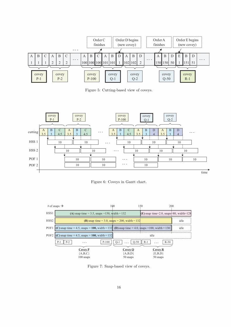
Table 1 introduces an example set of five orders. For this example, we assume that two HSS machines and

two POF machines are available and that their cycle time is 10 seconds. In this example, we define three

coveys. The first covey (Covey P ) consists of Orders A, B, and C. (This set of orders uses all four offloading

machines, since Order C has two plates per snap and thus requires both POF machines.) After 100 snaps of

this covey, Order C is completed and is replaced by Order D. Thus, Orders A, B, and D define the second

covey (Covey Q). After 50 snaps of Covey Q, Order A is completed (a total of 150 snaps) and is replaced by

Order E. Orders E, B, and D thus define the third covey (Covey R). The sequence of snaps produced by

the cutter and its relation to the coveys are described in Figure 5. The Gantt chart in Figure 6 illustrates

this schedule for each machine. The top row in the figure shows the schedule for the cutters, and the other

four rows show the schedule for each offloading machine.

Another useful representation of coveys is a snap-based view illustrated in Figure 7. This view specifies the

sequence of orders, their assignment to offloading machines, and the number of snaps to be produced of each

order and of each covey. In the example, Figure 7 shows that machine HSS1 first offloads 150 snaps of Order

A and then offloads 80 snaps of Order E, HSS2 offloads 200 snaps of Order B and then remains idle, POF1

offloads 100 snaps of Order C and 100 snaps of Order D (and is then idle), POF2 offloads 100 snaps of Order

C and is then idle for the rest of the time. In this view, it is easy to see the change of coveys; Covey P runs

for 100 snaps, followed by 50 snaps of Covey Q and 50 snaps of Covey R (and then 30 snaps of a fourth

covey consisting only of Order E).

For each covey, it is easy to calculate the required ribbon width. For ribbons with non-decreasing (non-

6

increasing) width, the ribbon width for a covey is the maximum width of a snap in that covey or any

preceding (subsequent) covey.

The volume of glass sent through the system per unit time is constant, as is the length and thickness of

a snap. Therefore, for a snap of given length and thickness, the time required to cut a snap is a function

of ribbon width. Consider a snap whose dimensions (length l, width w, and thickness t) is being cut on a

line that produces V volume of glass per second. Such a snap requires d = lwtV seconds of glass on a ribbon

of width w. However, if the snap is run on a wider ribbon of width w′ > w, the snap time increases to

d′ = lw′tV = dw′

w . (Note that although this means wider ribbon widths might help reduce cycle time scrap,

they simultaneously increase layout scrap, since l(w − w′)t volume of glass is wasted.)

Figure 8 gives a ribbon-based view of one cycle through each of the coveys P, Q, and R. It shows the amount

of scrap incurred in each covey. In Covey P , all three orders require the same snap width as the ribbon

width (132), so this covey has no layout scrap. In addition, the sum of snap times is 3.5 + 3.0 + 4.5 = 11

seconds, which exceeds the cycle time of the offloading machines. Therefore, Covey P does not have any

cycle time scrap. In Covey Q, the snap width of Order D is 130, but the ribbon width must remain 132

because Orders A and B require a ribbon width of at least. Thus, Covey Q incurs layout scrap corresponding

to the area of difference between 132 and 130, multiplied by the ribbon’s thickness. The sum of snap times

is 3.5 + 3.0 + 4.0 = 10.5 > 10 seconds, so this covey does not have any cycle time scrap. In Covey R, the

snap width of Order E is 128 and that of Order D is 130, but the ribbon width is 132. Therefore, Covey

R has layout scrap corresponding to these two areas times the ribbon’s thickness. The sum of snap times

is 2.0 + 3.0 + 4.0 = 9.0 seconds, which is less than the offloading machines’ cycle time of 10 seconds. Thus,

Covey R has cycle time scrap corresponding to the volume of glass produced in one second of idle time.

3 Solution Approach

Our heuristic approach to the float glass problem is in two phases:

1. Define the standard snap for each order by selecting the number and orientation of plates in the order’s

snaps.

2. Construct a schedule for cutting and offloading the correct number of each order’s standard snap in a

way that satisfies the operational restrictions and machine cycle time limitations.

7

3.1 Snap Construction

The first step in our algorithm is to create a standard snap for each order, so that each order is filled by

repeatedly cutting its standard snap. As mentioned earlier, all plates in a snap come from the same order.

Thus, for each order we only need to determine the orientation and the number of the plates in each snap.

Snap width is determined by these two factors.

There are only a few choices for each order. For example, to produce plates of size of 35 × 40 on a ribbon

with minimum and maximum width 100 and 140, the manufacturer can produce three plates or four plates

of dimensions 35× 40, or three plates of dimensions 40× 35 (see Figure 9).

The preference in snap construction is to have smaller variance in snap widths in order to reduce layout

scrap. Thus, we simply choose the rotation of a plate and the number of plates in a snap so that snap width

is closest to the average of the maximum and minimum ribbon widths in the shift. Since the snap width of

the last alternative is closest to 100+1402 , we would select it to be the order’s standard snap.

3.2 Constructing Cutting and Offloading Schedules

The scheduling phase of our approach has three main steps: preprocessing, construction, and local improve-

ments. The preprocessing steps help to balance the workload among machines. The construction step uses

a greedy scheme to construct an initial schedule. Finally, we use a number of local improvement schemes to

reduce scrap.

3.2.1 Preprocessing

We have two preprocessing steps.

(i) Splitting Long Orders:

At the end of a schedule, we found that because no other orders remain, a covey often consists of only one

or two long orders. Thus, the sum of the snap times of orders in the last coveys is less than the cycle time of

the offloading machines, which causes the schedule to have cycle time scrap. We refer to this phenomenon

as the end effect. The amount of cycle time scrap caused by the end effect often comprises a large portion

of a schedule’s total scrap.

As a pre-processing step, in order to reduce the size of large orders and hence reduce end effect, we split

8

orders with a large number of snaps into several sub-orders with fewer snaps. We can only apply this splitting

rule as long as the order is large enough to require multiple containers so as not to violate the packaging

constraint. For example, if an order of 2,000 snaps requires five containers, we can split it into one order

of 1,200 snaps (three containers) and one order of 800 snaps (two containers). Figure 10 illustrates how

splitting long orders contributes to decreasing the end effect.

(ii) Balancing between HSS and POF machines

If the assignment of orders to offloading machines is not balanced between the HSS and POF machines,

one machine type may be busy while the other type is idle, thus increasing the chance of incurring cycle

time scrap. Although some orders’ characteristics require them to be picked by a certain type of machine,

orders which satisfy the size requirements of both HSS and POF machines can be offloaded by either type.

For these orders, we decide the assignment of offloading machine type in order to minimize the difference

between the total number of snaps offloaded by HSS machines and the total number of snaps offloaded by

POF machines.

3.2.2 Construction

We use greedy construction algorithms to obtain initial schedules. Orders are prioritized according to some

characteristics (discussed below). By priority, they are then assigned to offloading machines in the following

way. If the sum of snap times in the current covey is less than the machine cycle time (which would result in

this covey having cycle time scrap), then it is myopically beneficial to add another order to the covey. Thus,

the next order in the priority list is assigned to that covey if a machine is available to offload it. Otherwise,

if the covey already has no cycle time scrap or if no machine is available, this covey is considered “full” and

the algorithm advances to the next covey. The process iterates until all orders are assigned.

Assume that the ribbon width is monotonically non-increasing. Then, wider orders should be produced

earlier; otherwise, narrow orders will incur layout scrap. Therefore, we first sort the orders in non-increasing

order of width.

It is not uncommon to have many orders of the same width. We have two different ways of breaking ties

between such orders, leading to two slightly-different construction heuristics. Both tie-breaking methods are

designed to help reduce the end effect.

One tie-breaking method is to produce orders with shorter snap times first, to save longer-snap-time orders

for coveys that might be subject to the end effect; in such a case, the cycle time scrap of the end effect

9

would be smaller. We refer to the heuristic using this tie-breaking method as the Width-Then-Time (WTT )

method.

A second tie-breaking method is to begin orders with more snaps first, so that these orders are less likely

to have long end effects. We refer to the heuristic using this tie-breaking method as the Width-Then-Snaps

(WTS ) method.

3.2.3 Local Improvement Algorithms

Once an initial schedule has been constructed, we use three local improvement methods, push-back, relocation,

and exchange. We first apply push-back to the initial schedule, followed by repeated application of relocation

and exchange until there is no more improvement in the yield ratio. Since the push-back algorithm can be

applied to improve any schedule, we apply it not only to the initial schedule, but also to all potential

relocation and exchange schedules before evaluating their yield ratio.

(i) Push-back of Orders:

The purpose of the push-back step is to eliminate as much of the end effect as possible. We try to push

backward (earlier in time) the orders located in the later coveys in order to combine them with orders of the

earlier coveys. This can reduce the number of snaps with few orders (and consequently shorter total snap

times) and decrease the total cycle time scrap at the end of a shift.

At each iteration, the algorithm pushes backward the orders in the last covey by the number of snaps in

that last covey. The push-back algorithm is repeatedly applied to the last covey of a schedule as long as the

covey currently incurs cycle time scrap and push-back is feasible.

Figure 11 shows an example of the push-back algorithm. In Figure 11 (a), the last covey of the current

schedule consists only of Order 8, and the number of snaps in this covey is δ1. So, the push-back algorithm

moves Order 8 leftward by δ1 snaps. As a consequence, Order 4 also gets pushed back δ1 snaps to make

room, creating the schedule in Figure 11 (b).

Assume now that sum of snap times of Order 7 and Order 8 is less than the machine cycle time. Then, the

schedule in Figure 11 (b) still has an end effect. Thus, we want to push back Orders 7 and 8 by δ2 snaps.

Orders 6 and 4 are also pushed backward to make room, resulting in the schedule shown in Figure 11 (c).

Figure 11 (c) shows that no end effect now exists, since the sum of snap times of Orders 5, 7, and 8 is greater

than the machine cycle time. However, even if there still was an end effect, no push-back could be done,

10

since there is no room to push Orders 8 and 4 backward on the first POF machine.

(ii) Relocation of Orders

The relocation algorithm iteratively selects an order and evaluates the benefit of changing its position in the

schedule. It tries to relocate the order to the starting point of each covey on each machine of the same type

as the order is currently on. For each possible relocation, we run the push-back algorithm (if necessary)

and then compute the yield ratio of the updated schedule. If the new yield ratio is higher than the yield

ratio before the relocation, then the new schedule is retained; otherwise, we return to the schedule before

the relocation. The algorithm cycles through all orders, attempting to relocate each one in turn, until a

complete cycle is made with no changes.

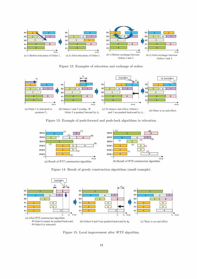
Figures 12 (a-1) and (a-2) illustrate one step of the relocation algorithm.

It might happen that when an order is relocated, it has enough snaps that its end overlaps the scheduled

start of the next order on the same machine. In such a case, we first apply a push-forward operation.

This operation might produce an increased end effect. Therefore, we apply the push-back algorithm after

each relocation of orders in order to remove as much of this end effect as possible. The push-forward and

subsequent push-back steps are illustrated in Figure 13.

(iii) Exchange of Orders

The exchange algorithm iteratively selects two orders and evaluates the benefit of exchanging their positions

in the schedule. Similar to relocation, orders are only exchanged between the same type of machine, and the

push-back algorithm is run after each potential exchange before calculating its yield ratio and comparing

with the yield ratio of the current schedule.

Figures 12 (b-1) and (b-2) illustrate one step of the exchange algorithm.

3.3 An Illustrative Example

In this section we illustrate our solution approach on an example problem instance. In this small example, we

assume that three HSS machines and three POF machines are available, all with cycle times of 10 seconds,

and that the minimum and maximum ribbon widths are 120 and 140 inches. Table 2 gives the dimensions

and number of plates in each order. For most orders, several snap constructions are possible. The selected

standard snap configuration for each order (the one whose width is closest to the average of the maximum

and minimum ribbon widths in the shift = 130) is denoted by an asterisk in the “selected snap” column in

11

Table 2 and listed in Table 3.

First, we assign orders to machine types. Because the number of plates per snap for Orders 1, 5, and 9 is

no more than three, we can assign those orders to POF machines. The other orders are assigned to HSS

machines.

Next, we create a priority list for each construction algorithm. For WTT, the list is (O4, O2, O3, O1, O6, O5,

O7, O8, O9), and for WTS the list is (O3, O4, O1, O2, O6, O5, O9, O8, O7). We then apply the construc-

tion algorithms to each list of orders. Figure 14 illustrates the schedules after applying the construction

algorithms.

The schedules generated by WTT and WTS have end effects that incur significant cycle time scrap. In

Figure 15, we would like to apply push-back to the schedule generated by WTS, but there is not enough

empty space to push Order 8 backward. However, during the relocation phase of local improvement, Order

8 gets relocated to the third HSS machine and then gets pushed back with Order 9.

Figure 16 shows a similar situation with the schedule generated by WTT. In Figure 16, Order 8 cannot be

pushed backward because there is not enough space, i.e. δ2 > δ3. However, when Order 8 and Order 7 are

exchanged, iterative push-back can be successfully applied to remove the end effect.

4 Computational Results

We tested our algorithms on actual shift data from the float glass plant we studied, and compared the yield

ratio from our solutions to the yield ratio from theirs. We also tested our algorithms on 250 additional

instances randomly generated from actual data. For the tests, our algorithms were implemented in C++

and executed on a Linux machine with two 2.4 GHz Processors and 2GB RAM.

We chose parameters to be close to the environment of the float glass plant: we assumed that four HSS

and four POF machines are available, that the cycle time of both POF and HSS offloading machines is 13

seconds, and that the ribbon width varies between 120 and 144 inches. The customer order data was exactly

the same as the company’s, but cannot be shown here due to confidentiality.

Table 4 shows the quality of the solutions for three actual instances of company order data. The three data

sets have 36, 40, and 49 orders. After splitting long orders (as described earlier), the number of orders

increases to 55, 46, and 57. In all three instances, the heuristics achieve more than 99.2%-99.6% yield in

less than 80 seconds, while the yield ratio of the actual shift schedule previously run by the company was

12

94.8%-97.4%.

For further validation, we conducted an experiment on randomly generated instances, with each order taken

from the pool of actual order data to make them realistic. We generated 250 instances, 50 each with 40, 50,

60, 70, and 80 orders. Tables 5 and 6 report heuristic yield ratios broken down by which pieces of the overall

solution approach are employed.

As the results shown in Tables 5 and 6 demonstrate, splitting long orders and using improvement heuristics

both have significant positive impact on the overall solution quality. Although balancing has only a small

effect on average, its improvement seems to be concentrated on instances where the overall solution quality

without balancing is worst. For example, in the instance where our heuristics perform worst, balancing

improves the yield ratio by over 3%. Thus, it is also an effective part of our overall solution approach.

Although the two construction algorithms WTT and WTS give very similar average solution quality, their

results on individual instances can sometimes vary in yield ratio. Therefore, since the algorithms run quickly

relative to the required solution time, we recommended to the manufacturer that when possible, they use

both algorithms and select whichever of the two schedules has a higher yield ratio. Table 7 shows the results

of using this strategy, which improves performance by 0.1%. This strategy has been implemented in the

manufacturing facility.

ACKNOWLEDGMENT The authors would like to thank the anonymous glass manufacturer for their

support of this collaborative work.

References

[1] Dash S, Kalagnanam J, Reddy C, Song SH. Production Design for Plate Products in the Steel Industry.

IBM Journal of Research and Development 2007;51: 345–362.

[2] Gilmore P, Gomory R. A Linear Programming Approach to the Cutting Stock Problem. Operations

Research 1961;9: 849–859.

[3] Gilmore P, Gomory R. A Linear Programming Approach to the Cutting Stock Problem–Part II. Oper-

ations Resesearch 1963;11: 863–888.

[4] Gupta JND, Tunc EA. Schedules for a Two Stage Hybrid Flowshop with Parallel Machines at the

Second Stage. Int. J. Prod. Res. 1991;29: 1489–1502.

13

[5] Grenzebach Maschinenbau GmbH. “Glass Technology: Robot.” Retrieved from

http://www.grenzebach.com/index.php/eng/produkthauptordner/glas technologie/roboter

[6] Linn R, Zhang W. Hybrid Flow Shop Scheduling: A Survey. Computers and Industrial Engineering,

1999;37: 57–61.

[7] Na B, Ahmed S, Nemhauser GL, Sokol J. Two-Stage Hybrid Flow Shop Scheduling with Covering

Constraints ISyE working paper, in preparation.

[8] Pinedo ML. Scheduling: Theory, Algorithms, and Systems. 3rd Edition: Springer, 2008.

[9] Tangram Technology Ltd. “Float glass production.” Retrieved from http://www.tangram.co.uk/TI-

Glazing-Float%20Glass.html

Figure 1: Basic float glass manufacturing process [9].

layout

scrap

ribbon width

snap width

cycle time

scrap

a plate

a snapx-cuts

y-cuts

Figure 2: Terminology of a float line.

14

(a) High-speed-stacker (HSS) machine (b) Pick-on-the-fly (POF) machine

Figure 3: Types of offloading machines [5].

cutting

offloading 1

time

(b) Interspersing snaps of another order can decrease cycle time scrap.

10 10

3

10 10 10

offloading 2

6 63

10

10

cutting

offloading 1

time

(c) If interspersed snaps create a cycle at least as long as machines require, there is no cycle time scrap.

8

10 10 10

3

10 10

offloading 2

3 8 83

10

cycle time scrap = 1a cycle

no scrapa cycle

cutting

offloading 1

time

(a) Cutting snaps of a single order consecutively normally incurs significant cycle time scrap.

3

10 10 10

3 3 3

10

cycle time scrap = 7a cycle

6

10

3

36 3

8

10

Figure 4: Gantt chart showing how cycle time scrap is incurred.

15

A

1- - -

B

1

C

1

A

2

B

2

C

2

A

100

B

100

C

100

A

101

B

101

D

1

A

102

B

102

D

2

covey

P-1

covey

P-2

covey

P-100

covey

Q-1

covey

Q-2

- - -A

150

B

150

D

50

covey

Q-50

E

1

B

151

D

51

covey

R-1

- - -

- - -

Order C

finishes

Order D begins

(new covey)

Order A

finishes

Order E begins

(new covey)

Figure 5: Cutting-based view of coveys.

cutting

HSS 1

time

HSS 2

A

3.5

B

3

A

3.5

C

4.5

10

10

10

10

10

10

A

3.5

B

3

10

10

A

3.5

C

4.5

10 10

10

POF 1

covey

P-1

covey

P-2

covey

P-100

covey

Q-1

covey

Q-2

- - -

- - -

- - -

- - -

- - -C

4.5

B

3

POF 2

B

3

D

4

A

3.5

B

3

D

4

10

10 10 10

10 10 10- - -

Figure 6: Coveys in Gantt chart.

100# of snaps à

Covey P

{A,B,C}

100 snaps

Covey Q

{A,B,D}

50 snaps

150

P-1 P-100

Covey R

{E,B,D}

50 snaps

200

(A) snap time = 3.5, snaps =150, width = 132

(B) snap time = 3.0, snaps = 200, width = 132

(C) snap time = 4.5, snaps = 100, width = 132 (D) snap time = 4.0, snaps =100, width = 130

(E) snap time=2.0, snaps=80, width=128HSS1

HSS2

POF1

POF2

P-2 Q-1 Q-50. . . . . . R-1 R-50. . .

(C) snap time = 4.5, snaps = 100, width = 132 idle

idle

idle

Figure 7: Snap-based view of coveys.

16

(C) snap time=4.5, width=132

(A) snap time=3.5, width=132

(B) snap time=3.0, width=132

(D) snap time = 4.0,

width = 130(D) snap time = 4.0,

width=130

(E) time=2.0, width=128

layout

scrap

layout

scrap

cycle time

scrapribbon width = 132 ribbon width = 132 ribbon width = 132

Covey P Covey Q Covey R

(a) no cycle time scrap

and no layout scrap

(b) no cycle time scrap but

layout scrap

(c) both cycle time scrap

and layout scrap

sum of snap

times = 11.0

sum of snap

times = 10.5sum of snap

times = 9

(A) snap time=3.5, width=132

(B) snap time=3.0, width=132

(B) snap time=3.0, width=132

Figure 8: Scrap according to different covey construction.

snap width = 120

40

35

40 4035 35 35 35

40

snap width = 140(c) three plates of (40 x 35)

after rotation(b) four plates of (35 x 40)

35 35 35

40

snap width = 105

(a) three plates of (35 x 40)

Figure 9: Snap construction alternatives.

1

2

4

3

5 6H1

H2

H3

P1

P2

End Effect

(a) Order 2 has a large number of snaps.

à Large end effect.

snap

4

7

1

4

3

5 6

H1

H2

H3

P1

P2

End Effect

snap

4

7

2-A

2-B

(b) Order 2 splits into Order 2-A and Order 2-B.

à Small end effect.

Figure 10: Splitting long orders.

1

2

4

3

5

6 7

H1

H2

H3

P1

P2

End Effect

δ1

End Effect

δ2

No End Effect

(a) Order 8 is pushed backward by δ1.

à Orders 4 and 8 move together(b) Orders 7 and 8 are pushed backward by δ2. (c) Push-back removes end effect.

snap

4

8

1

2

3

5

6 7

H1

H2

H3

P1

P2

snap

4

8

1

2

4

3

5

6 7

H1

H2

H3

P1

P2

snap

4

84

Figure 11: Iterative Push-back algorithm.

17

(a-1) Before relocation of Order 1. (a-2) After relocation of Order 1. (b-1) Before exchange between

Orders 1 and 5.(b-2) After exchange between

Orders 1 and 5.

1

2

4

3

5

6 7

H1

H2

H3

P1

P2

snap

4

8

1

2

4

3

5

6 7

H1

H2

H3

P1

P2

snap

4

8

1

2

4

3

5

6 7

H1

H2

H3

P1

P2

snap

4

8

1

2

4

3

5

6 7

H1

H2

H3

P1

P2

snap

4

8

Figure 12: Examples of relocation and exchange of orders.

(a) Order 1 is relocated to

position P1.

δ3

δ4

(b) Orders 1 and 5 overlap. à

Order 5 is pushed forward by δ3.

End Effect

(c) To remove end effect, Orders 1

and 5 are pushed backward by δ4 .

No End Effect

(d) There is no end effect.

P1

1

2

4

3

5

6 7

snap

4

8

1

2

4

3

5

6 7

H1

H2

H3

P1

P2

snap

4

8

1

2

4

3

5

6 7

snap

4

8

1

2

4

3

5

6 7

snap

4

8

H1

H2

H3

P1

P2

H1

H2

H3

P1

P2

Figure 13: Example of push-forward and push-back algorithms in relocation.

3

1

1

1

2

4 6

5

5

9

8

7

HSS1

HSS2

HSS3

POF1

POF2

POF3

2

3

1

1

1

4

6

5

5

7

8

9

(1)

(2)

(3)

(4)

(7)

(5)

(6)

(8)

(9)

(1)

(2)

(3)

(4)

(5)

(6)

(7)

(8)

(9)

(a) Result of WTT construction algorithm. (b) Result of WTS construction algorithm.snap snap

HSS1

HSS2

HSS3

POF1

POF2

POF3

Figure 14: Result of greedy construction algorithms (small example).

End Effect

δ6

snap

3H1

H2

H3

P1

P2

P3

1

1

1

2

4 6

5

5

9

8

7

δ7

snap

3H1

H2

H3

P1

P2

P3

1

1

1

2

4 6

5

5

9

8

7

snap

3H1

H2

H3

P1

P2

P3

1

1

1

2

4 6

5

5

9

8

7

s2s1 s2s1 s1

(a) After WTS construction algorithm

à Order 8 cannot be pushed backward.

à Order 8 is relocated.(b) Orders 8 and 9 are pushed backward by δ6. (c) There is no end effect.

δ6

Figure 15: Local improvement after WTS algorithm.

18

H1

H2

H3

P1

P2

P3

2

3

1

1

1

4

6

5

5

7

8

9

End Effect

δ1

s2s1snaps3

H1

H2

H3

P1

P2

P3

2

3

1

1

1

4

6

5

5

7

8

9

s2s1snap

δ2δ3

H1

H2

H3

P1

P2

P3

2

3

1

1

1

4

6

5

5

7

8

9

s2s6snap

δ4

H1

H2

H3

P1

P2

P3

2

3

1

1

1

4

6

5

5

7

8

9

s5 s6snap

δ5

s5

s4

s4

H1

H2

H3

P1

P2

P3

2

3

1

1

1

4

6

5

5

7

8

9

s5 snap

(a) After WTT construction algorithm

à Order 9 is pushed backward by δ1.

(b) Order 8 cannot be pushed backward by δ2

because δ2 > δ3. à Orders 7 and 8 are exchanged.

(d) Orders 8 and 9 are pushed backward by δ5.

à Orders 1, 5, and 9 move together.(e) There is no end effect.

(c) Order 9 is pushed backward by δ4.

Figure 16: Local improvement after WTT algorithm.

Table 1: Five orders are to be produced.

index snap time # of snaps snap width plates per snap offloading machine

A 3.5 150 132 3 HSS 1B 3.0 200 132 5 HSS 2C 4.5 100 132 2 POF 1 & 2D 4.0 100 130 1 POF 1E 2.0 80 128 7 HSS 1

19

Table 2: Alternatives for snap construction (small example).

Given customer orders Alternatives for snap construction

index dimension total plates width × height plates snap width selected snap

1 44 × 50 600 44 × 50 3 132 *

2 30 × 33 600 30 × 33 4 12033 × 30 4 132 *

3 22 × 45 2,400 22 × 45 6 132 *45 × 22 3 135

4 16.5 × 25 2,000 16.5 × 25 8 132 *25 × 16.5 5 125

5 60 × 65 200 60 × 65 2 12065 × 60 2 130 *

6 32.5 × 35 800 32.5 × 35 4 130 *35 × 32.5 4 140

7 16 × 20 800 16 × 20 8 128 *16 × 20 9 14420 × 16 6 12020 × 16 7 140

8 30 × 32 800 30 × 32 4 12032 × 30 4 128 *

9 55 × 128 250 128 × 55 1 128 *

Table 3: Result of snap construction (small example).

index total plates snap width width × height plates # of snaps snap time

1 600 132 44 × 50 3 200 5.02 600 132 33 × 30 4 150 3.03 2,400 132 22 × 45 6 400 4.54 2,000 132 16.5 × 25 8 250 2.55 200 130 65 × 60 2 100 6.06 800 130 32.5 × 35 4 200 3.57 800 128 16 × 20 8 100 2.08 800 128 32 × 30 4 200 3.09 250 128 128 × 55 1 250 5.5

Table 4: Computational results on actual data

Actual shift schedule Balancing + WTT + local search Balancing + WTS + local search

Instance Yield ratio(%) Yield ratio (%) Time (sec) Yield ratio(%) Time (sec)

Data Set 1 95.3 99.6 70 99.2 79Data Set 2 97.4 99.2 26 99.4 23Data Set 3 94.8 99.3 63 99.5 51

20

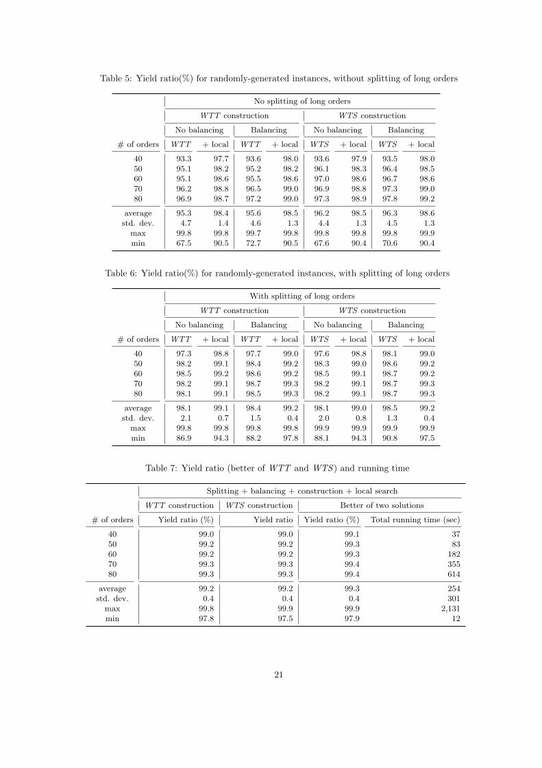
Table 5: Yield ratio(%) for randomly-generated instances, without splitting of long orders

No splitting of long orders

WTT construction WTS construction

No balancing Balancing No balancing Balancing

# of orders WTT + local WTT + local WTS + local WTS + local

40 93.3 97.7 93.6 98.0 93.6 97.9 93.5 98.050 95.1 98.2 95.2 98.2 96.1 98.3 96.4 98.560 95.1 98.6 95.5 98.6 97.0 98.6 96.7 98.670 96.2 98.8 96.5 99.0 96.9 98.8 97.3 99.080 96.9 98.7 97.2 99.0 97.3 98.9 97.8 99.2

average 95.3 98.4 95.6 98.5 96.2 98.5 96.3 98.6std. dev. 4.7 1.4 4.6 1.3 4.4 1.3 4.5 1.3

max 99.8 99.8 99.7 99.8 99.8 99.8 99.8 99.9min 67.5 90.5 72.7 90.5 67.6 90.4 70.6 90.4

Table 6: Yield ratio(%) for randomly-generated instances, with splitting of long orders

With splitting of long orders

WTT construction WTS construction

No balancing Balancing No balancing Balancing

# of orders WTT + local WTT + local WTS + local WTS + local

40 97.3 98.8 97.7 99.0 97.6 98.8 98.1 99.050 98.2 99.1 98.4 99.2 98.3 99.0 98.6 99.260 98.5 99.2 98.6 99.2 98.5 99.1 98.7 99.270 98.2 99.1 98.7 99.3 98.2 99.1 98.7 99.380 98.1 99.1 98.5 99.3 98.2 99.1 98.7 99.3

average 98.1 99.1 98.4 99.2 98.1 99.0 98.5 99.2std. dev. 2.1 0.7 1.5 0.4 2.0 0.8 1.3 0.4

max 99.8 99.8 99.8 99.8 99.9 99.9 99.9 99.9min 86.9 94.3 88.2 97.8 88.1 94.3 90.8 97.5

Table 7: Yield ratio (better of WTT and WTS ) and running time

Splitting + balancing + construction + local search

WTT construction WTS construction Better of two solutions

# of orders Yield ratio (%) Yield ratio Yield ratio (%) Total running time (sec)

40 99.0 99.0 99.1 3750 99.2 99.2 99.3 8360 99.2 99.2 99.3 18270 99.3 99.3 99.4 35580 99.3 99.3 99.4 614

average 99.2 99.2 99.3 254std. dev. 0.4 0.4 0.4 301

max 99.8 99.9 99.9 2,131min 97.8 97.5 97.9 12

21