Moshood Abdulwahab

OPTIMIZATION OF CO2 REMOVAL IN AN ABSORP-

TION-DESORPTION UNIT

Thesis

CENTRAL OSTROBOTHNIA UNIVERSITY OF APPLIED

SCIENCES

Degree Programme in Chemistry and Technology

September 2010

ABSTRACT

CENTRAL OSTROBOTHNIA UNI-

VERSITY OF APPLIED SCIENCES

Date

September 2010

Author

Moshood Abdulwahab

Degree programme

Chemistry and Technology

Name of thesis

Optimization of CO2 removal in an absorption-desorption unit

Instructor

Staffan Borg

Pages

[61 + 5 APPENDICES]

Supervisor

Staffan Borg

This review presents the optimization of monoethanolamine(MEA) regeneration in a pilot

scale CO2-MEA absorption-desorption unit. The goals of the thesis were to identify the

variables affecting the stripping process and determine their optimum combination, and

to give suggestions necessary for the improvement of the stripper’s capacity.

A thorough perusal of the literature on the phenomena and the equipment was carried

out to adequately understand the variables in action. Experiment trials were also con-

ducted, in line with the Taguchi’s method dictates, to determine the optimum combina-

tion of the tunable variables in the system.

The literature survey revealed a number of factors, four of which were further investi-

gated to determine the optimum. The optimum condition for the washing liquid regenera-

tion was determined. Also, two retrofitting recommendations were given to improve the

capacity of the equipment.

Key words

Absorption, analysis of variance (ANOVA), design of experiment, desorption, monoetha-

nolamine (MEA), orthogonal array, packed column, Taguchi’s method.

TABLE OF CONTENTS

1 INTRODUCTION ........................................................................................................... 1

2 THEORETICAL BACKGROUND ................................................................................ 4

2.1 Gas absorption ........................................................................................................... 4

2.2 Washing liquid ........................................................................................................... 5

2.3 Gas desorption ........................................................................................................... 8

2.4 The packed column ................................................................................................... 9

2.4.1 Packed column internals .................................................................................. 11

2.4.2 Absorption-desorption in the packed column ............................................. 14

2.4.3 Packed column design ..................................................................................... 16

3 DESIGN OF EXPERIMENT ......................................................................................... 31

3.1 The Taguchi approach to quality improvement ................................................. 32

3.2 Designing experiment the Taguchi way .............................................................. 34

3.2.1 Brainstorming .................................................................................................... 35

3.2.2 Designing and executing ................................................................................. 36

3.2.3 Analysis of results ............................................................................................. 38

3.2.4 Confirmatory test .............................................................................................. 43

4 EXPERIMENTATION .................................................................................................. 45

4.1 Equipment description ........................................................................................... 45

4.2 Experimental procedure ......................................................................................... 47

5 DATA AND CALCULATIONS .................................................................................. 51

6 DISCUSSION ................................................................................................................. 57

REFERENCES

APPENDICES

1

1 INTRODUCTION

In the past few decades, environmental consciousness has encouraged a new creed

in sciences and engineering dubbed with appellations formed from their parental

disciplines prefixed with green, for example, Green Chemistry and Green Engi-

neering. This creed promotes the maintenance of greenness in the practice of

sciences and engineering, that is, the integration of environmental and economical

aspects of the practices. This belief is born out of the realization of the environ-

mental impacts of the anthropogenic pollutions—pollutions resulting from human

actions, chiefly from the industrial, in the past.

Global warming—a phenomenon which has been the subject of discourse in the

media for years—is one of the undesired consequences attributed to anthropogen-

ic actions. Global warming is simply the increase in the overall atmospheric tem-

perature of the earth, leading to changes in climatic conditions. Alarms have been

raised about the consequences of the earth’s temperature increment; among the

recent ones is the melting of the glacial ices, especially in the northern regions of

the globe whose inhabitants loved dearly the winter season. By the way of ex-

plaining this warming phenomenon, hindrance to the emission of certain electro-

magnetic radiations caused by the concentration of the atmosphere with the so

called greenhouse gases has been proposed. The inhibiting process itself is termed

greenhouse effect. The greenhouse gases include carbon dioxide, CO2, methane,

ozone, chlorofluorocarbons, and water vapour. CO2 has been regarded as a major

contributor because of its large flaring from power plants and the chemical indus-

try. In order to combat this, governments have introduced strict measures on the

allowed emissions. Hence, the need for CO2 capturing technologies has increased.

2

The CO2 capturing technologies include gas absorption with solvents, gas adsorp-

tion using solids, membranes sieving, and cryogenic methods. Based on practical

applications, gas absorption is far more cost effective compared to any other cap-

turing or sequestering technology. Thus its installation dwarfs any other. Gas ab-

sorption is a famous unit operation in the chemical industry, second to only distil-

lation, in which a liquid solvent is utilized to absorb one or more components of a

gas mixture. The streams are countercurrently contacted in a packed column—a

cylindrical tower equipped with solids materials in it. This unit is usually operated

in a closed loop with a second tower in which the loaded solvent is regenerated

and returned to the first one.

In a pilot scale CO2-MEA absorption-desorption unit built in the Central Ostro-

bothnia University of Applied Sciences laboratory, the desorbing column is ob-

served to flood frequently, a phenomenon which is known to grow the pressure

drop and to reduce the desorption rate. This brings about a CO2 build up in the

whole system, significantly reducing the amount of CO2 absorbed in the absorber.

As the efficiency of the whole unit is tied to the effective liquid regeneration in the

stripping tower, it is important to optimize the desorption process.

The goal of this thesis is to study the variables affecting the regeneration of the

washing liquid, MEA, in the desorber of the pilot scale equipment mentioned

above and then propose recommendations to help improve the capacity of the

stripper; and also to determine the optimum condition of the stripping process at

hand through experimentation. For the scope of this research, attention would be

focused on the system at hand, that is, the study will leave out the different types

of ways in which absorption can be carried out and concentrate on the way it is

been done in the laboratory under study-the use of packed column. To start with,

this review will begin with the discussion on the gas absorption phenomenon and

3

the equipment used in this study, the packed column, and then delving into the

principles upholding experimental design; specifically the Taguchi’s as this ap-

proach will be utilize in the study. Information on the execution, results and calcu-

lations involving the experiments will follow, and lastly, discussion and recom-

mendations regarding the unit in question.

As regards the purpose of this work, the research questions listed below are for-

mulated in order to further buttress the aim of the work.

1. What are the variables affecting MEA regeneration in the de-

sorber

2. How can MEA regenerating capacity of the stripper be im-

proved

3. What is the optimum MEA regenerating condition of the ab-

sorption-desorption unit

4

2 THEORETICAL BACKGROUND

Under this heading, the presentation and discussion of facts about the phenome-

non of gas absorption and the use of the packed column to achieving the feat will

be discussed.

2.1 Gas absorption

In chemical engineering, gas absorption (also called gas washing or scrubbing)

refers to the unit operation utilized for sequestering one or more components of

interest in a gas mixture. The separation is achieved by the introduction of a liquid

phase, usually called washing liquid or solvent, with strong affinity for the desired

component in contact with the gas mixture inside an equipment that allow for

adequate interaction between the phases. Hence, the introduced liquid phase be-

comes loaded with the desired component(s) while the gas phase mainly contains

the inert component(s). (Green & Perry 2008, 14-6; McCabe, Smith & Harriott 2005,

565; Seader & Henley 2006, 193.)

This concept has considerable applications in the chemical industry, for instance,

treatment of emissions from power plants that uses fossil fuel, CO2 and H2S re-

moval in natural gas processing, petroleum refinery, and coal gasification so as to

avoid corrosion in the pipes and souring of the oil. CO2 absorption makes a sig-

nificant percentage of the gas absorption phenomenon because of the increase re-

strictions on its emission and the need for maximum usage of materials to mini-

mize costs.

5

Central to the functionality of this process is adequate mass transfer, which in turn

depends on proper interaction between the phases involved. With the latest de-

velopment on ground, this interaction is achieved in five different ways with five

different devices namely packed column, tray or plate column, bubble tower, cen-

trifugal contactor, and the spray tower (Seader & Henley 2006, 196-200). However,

it is worthy of mentioning that researchers are working on novel state of the art

equipment, the fibre hollow contactor, which is supposed to be advantageous over

the conventional ones though not yet commercialized (Li & Chen 2005;

Koonaphapdeelert, Wu & Li 2009). The packed tower and plate column are usu-

ally the contending options to choose from when the necessary design calculations

and economical considerations are critically examined side by side with installa-

tion requirements. The spray column usually finds usage when the required gas

absorption process is very easy to achieve, while the bubble column is employed

when a considerable residence time is required for the interaction due to either

slow chemical reaction or very low solubility of the gas in the solvent. The cen-

trifugal contactor is used when the required height of the equipment is not avail-

able or when a fast result is needed. (Seader & Henley 2006, 196-200; Zenz 1980,

289-307.)

2.2 Washing liquid

The liquid phase employed in the gas absorption process is commonly referred to

as the washing liquid or solvent. In choosing the washing liquid, ‘‘preference is

given to solvents with high solubilities for the target solute and high selectiv-

ity....low volatility, low cost, low corrosive tendencies, high stability, low viscosity,

low tendency to foam, and low flammability.’’(Green & Perry 2008, 14-7.)

6

Liquid interaction with the gas phase can either be physical or chemical. Weak

bonding forces between the fluids molecules are responsible for withholding the

gases in physically absorbing solvent, whereas in the chemical absorption either a

reversible or an irreversible reaction consumes the gases for the formation of a

chemical complex. In either case, a change in the conditions of state can result in

the release of the absorbed gas by the washing liquid. Chemically absorbing sol-

vents are known to have higher solubilities compared to their counterpart as a re-

sult of the reaction taking place when the phases adequately contact each other. As

the solutes disappear in the liquid phase, a chance is created for more solutes to be

dissolved. ( McCabe et. al. 2005, 591-604; Strelzoff 1980, 309-310.)

7

A comparative study of the physical and chemical absorption using the solubility

data of CO2-propylene carbonate (PC) and CO2-monoethanolamine (MEA) under

the condition of two different temperatures yields the graph below.

GRAPH 1. Linear scale plot of solubility of CO2 in 30 weight% monoethanolamine

(MEA) and propylene carbonate (PC) (adapted from Green & Perry 2008, 14-8)

Graph 1 shows a plot of the percentage by weight of CO2 in the liquid phase (solu-

bility) on the ordinate against the partial pressure of the CO2 in the gas phase on

the abscissa. Bearing in mind that pressure and mole have a direct relation, the

plot on the x-axis is an indication of the amount of CO2 to be absorbed. Hence, it

can be concluded from the graph that physically absorbing solvents are more ef-

fective when dealing with gas mixture with high amount or partial pressure of

CO2, the reverse is true for chemical absorption. These conclusions are drawn as a

0

5

10

15

20

25

30

0 2 4 6 8 10 12 14

we

igh

t %

CO

2 in

Liq

uid

PCO2(kPa)

PC,100oC PC, 40oC MEA, 40oC MEA, 100oC

8

linear relationship is observed between the plots (CO2-PC) for physical absorption,

indicating a continuous increase in solubility as gas phase concentration rises.

Meanwhile, the chemically absorbing plots (CO2-MEA) exhibit higher solubility at

low concentration but the solubility remains circa constant as the x-axis plot

grows. (Green & Perry 2008, 14-7—14-8; Strelzoff 1980, 308-313.)

Furthermore, temperature increase is observed to decrease the solubility as seen

from the isotherms in both cases. Thus, a consideration of the conditions of a gas

mixture, most importantly the solute’s partial pressure or amount and tempera-

ture, in addition to the good solvent qualities aforementioned, are paramount to

the choice of solvent to be employed in the gas absorption unit. In addition, pres-

sure reduction can be utilized to strip a physically absorbing washing solvent as it

absorbs at a high pressure. This pressure swing application is by far cheaper than

that of the temperature swing. The importance of the choice of solvent cannot be

overemphasized as it is primary to the cost and greenness of the process. (Green &

Perry 2008, 14-7—14-8; Strelzoff 1980, 308-313.)

2.3 Gas desorption

Desorption, also known as stripping, is the direct opposite of gas absorption. Here,

the loaded washing liquid from the absorption column is regenerated, that is,

stripped off the absorbed solute. Similarly as in the absorption process, a new

phase, usually gaseous, that acts as the stripping agent has to be introduced. De-

pending on the nature in which the absorbed solute(s) is (are) needed; either pris-

tine or impure, the choice of stripping agent is made to suit the desire. When the

solute is to be captured, probably due to the environmental restrictions on its

emission or its usefulness, steam is usually employed as the gas phase. This is

9

rather expensive but the choice strongly relies on the weight of the benefits or

regulations on ground. On the other hand, when it is not necessary to recover the

solute in a pure state, either to be flared or captured as well, a cheaper gas flow is

made use of as the stripping agent. Air is commonly used because of its availabil-

ity. (McCabe et. al. 2005, 590-591.)

Desorption is run in a continuous closed loop, hand in hand with the gas absorp-

tion process. The regenerated or lean solvent from the desorber is repumped into

the absorber as a fresh solvent. This fact underlines the importance of effective

regeneration in the desorber as its core to the overall efficiency of the unit as a

whole. The packed column as well is commonly in use for the process of desorp-

tion. (Seader & Henley 2006, 193.)

2.4 The packed column

The packed column/tower is a device employed in the chemical industry for a

number of mass transfer operations. Common operations carried out with the

packed column include distillation, gas absorption and desorption, and leaching.

From an external view, the packed column is no more than a cylindrical tower

equipped with two openings at the top and bottom to allow for liquid and gas

streams entry and exit. These streams are arranged countercurrently with the liq-

uid flow’s inlet and outlet situated at the top and bottom respectively. The con-

verse is true for the gas flow. An internal reconnoiter from top to down reveals

some additional internal features such as liquid distributor, section(s) of packings

supported above and below with a support plate, liquid collectors, and liquid re-

distributors. Graph 2 shows a packed column with its internals visible. (Green &

Perry 2008, 14-53; McCabe et. al. 2005, 565-566; Seader & Henley 2006, 198.)

10

GRAPH 2. An internal view of the packed column (from Sulzer Chemtech’s inter-

nals for packed column)

Liquid Inlet

Distributor

Structured Packing

Packings Support

Redistributor

Bed Limiter

Random Packing

Packings Support

Gas Inlet

Gas Outlet

11

2.4.1 Packed column internals

The column internals are discussed in this heading. The distributor is put in place

to distribute the inlet liquid flow evenly across the packing’s surface. The liquid

inlet feed is usually directed to the distributor, which then effects the distribution.

The distributor plays a vital role in the overall efficiency of the column, especially

in columns with a large diameter, as its presence is necessary to provide adequate

contact of the phases. (Green & Perry 2008, 14-73; McCabe et. al. 2005, 565; Saint-

Gobain Norpro 2001; Seader & Henley 2006, 198.)

Packings are solid objects gathered in sections inside the packed column. They are

available in different materials and shapes from which they are usually named, for

example, ceramic Raschig ring. Packings are shaped with the goal of increasing

the interfacial surface area and reducing the pressure drop as fluids flow through

them. The material with which packings are made of determines their wettability,

corrosion resistance, strength and price. All of these are significant factors that are

considered when making choice of packing. The oldest packings used are the Ra-

schig rings and the Berl saddles. These have been largely replaced by varieties of

design, in terms of structural improvement, to handle better flow capacity, to pro-

duce lower pressure drop, and to exhibit much more surface area for fluid interac-

tion. Some of the existing packings types are shown in Graph 3 below. (Green &

Perry 2008, 14-53—14-54; McCabe et. al. 2005, 565-567; Seader & Henley 2006, 198-

199.)

12

GRAPH 3. Various packing types( Seader & Henley 2006, 199)

An inverse proportional relationship exists between packing size and pressure

drop in the column, also with the mass transfer performance. However, a high

mass transfer rate and low pressure drop are the required conditions in view of

the performance of the column and the cost of pumping respectively. The mass

transfer advantage rendered by smaller packing is said to be minimal; conse-

quently, larger packings are favoured because of their lower pressure drop edge.

The general rule of thumb in choosing packing size is that packing size should be

about one-eighth of the column’s diameter (McCabe et. al. 2005, 568-9; Seader &

Henley 2006, 198-199). Adherence to this rule is said to eliminate channelling, the

maldistribution of liquid throughput, which is a major problem in towers with a

large diameter. Additionally, as liquid distribution is vital to the efficiency of mass

transfer in packed columns, sections of packings allotted with distributors or re-

13

distributors are used especially in tall columns also to ensure even distribution.

According to Saint-Gobain Norpro’s packed tower internals guide (Saint-Gobain

Norpro 2001), sections of packings should not be more than fifteen times the col-

umn diameter and contain less than twenty theoretical stages, while Zenz (1980)

proposes the smaller one of either five times the column’s diameter or ten feet

packings height. (McCabe et. al. 2005, 568-9; Seader & Henley 2006, 198-199; Zenz

1980, 289-307.)

Packings can be either dumped or arranged into the columns. The former is re-

ferred to as random packing while the latter can either be stacked or structured

packing. Stacked packings are arranged in the column by hand, whereas struc-

tured packings are made pre-arranged by the manufacturer. Structured packings

usually give less pressure drop compared to random packings, but random pack-

ing gives higher mass transfer. This statement is consistent with the results of the

experiments conducted by Longo and Gasparella (2009) on desiccant regeneration

performed with both random and structured packings. Under their experimental

conditions, structured packings gave a 65-75% lower pressure drop while random

packing had 20-25% higher regeneration performance. Apparently, due to these

facts, structured packing can handle bigger streams, but it is expensive as com-

pared to its counterpart. This is why random packing is found to be more cost ef-

fective in the smaller towers. When dealing with very high flows, structural pack-

ings are essential for the sole reason of extending the flooding capacity and to

minimize the energy spent on pumping. (Green & Perry 2008, 14-53—14-54;

McCabe et. al. 2005, 568-604; Seader & Henley 2006, 198-199; Longo & Gasparella

2009.)

The packing support is the seat on which the packings gain their stance. Packing

supports commonly possess a netlike surface to allow for the passage of the gas

14

phase upward the column. Similar in structure is the bed limiter which is placed

on top of the packings to keep them orderly when gas flow is increased close to or

above the fluidization value. Every section of packings has a packing support on

which to stand and a limiter to maintain order above it. (Saint-Gobain Norpro

2001; Seader & Henley 2006, 198.)

In order to avoid channelling, the idea of using sections of packings was intro-

duced. A recommendation as to the height of packings to be utilized at a section

has been mentioned earlier. The collector serves to gather the downward coming

liquid phase from the upper packing section and leads it to the redistributor which

wets the next packing section. (Green & Perry 2008, 14-53—14-54; McCabe et. al.

2005, 568-604; Saint-Gobain Norpro 2001; Seader & Henley 2006, 198-199.)

2.4.2 Absorption-desorption in the packed column

Having explained the absorption and the desorption phenomena in the early part

of this chapter, and described the equipment, packed column, which can be em-

ployed for both processes, it is imperative to talk about how the duo phenomena

are united in the twin towers working together as a continuous process to forming

the unit operation dubbed gas absorption. The gas absorption unit normally con-

sists of two towers; one for absorbing the target gas, the absorber or scrubber, and

the other for regenerating the used solvent, the stripper or desorber.

The absorber is a packed column with all the ancillaries aforementioned. On the

introduction of the solvent from the top of the column, the distributor spreads it as

evenly as it can over the cross sectional area of the packings directly below it. As

the solvent is pulled down by gravity through the sections of packing, the

15

throughput is broken into droplets and spreads around the interfacial area of the

packing; simultaneously, the inlet gas mixture to be purified would make its way

up from the bottom of the column also through the packings (Zenz 1980, 289-307).

When the fluids meet at the surface area provided by the packings, they interact

and mass transfer of the target gas will take place at that instant. This happens

continuously as the solvent moves through the packings. Consequently, the liquid

phase increases in the amount of the absorbed gas down the column whereas the

gas phase reduces in its concentration of the solute up the column. Hence, the out-

going gas is purified, or at least contains less of the target gas; on the other hand,

the outgoing liquid phase is loaded with the absorbed gas. The need to regenerate

and reuse the spent washing liquid usually invokes the use of a second tower,

known as the desorber. (CO2CRC 2010; McCabe et. al. 2005, 565-569; Seader &

Henley 2006, 198; Zenz 1980, 289-307.)

The desorber as well is merely a packed tower except that it is equipped with a

reboiler for the production of steam as the gas phase when the target gas is to be

captured purely. When the target gas is not needed pure and there exist no restric-

tion on its emission, a cheaper gas can be utilized. Just like in the absorber the liq-

uid inlet, the loaded solvent in this case, is from the top the column while the gas

phase, the stripping agent is from the bottom. In the same manner, they meet on

the packings and the absorbed gas is released into the gas phase. Here, the de-

sorbed gas is collected on its way out of the column while the fresh solvent is sent

back to the absorber, making a cyclic process. (CO2CRC 2010; McCabe et. al. 2005,

565-569; Seader & Henley 2006, 198; Zenz 1980, 289-307.)

Generally, a state of high pressure and low temperature favours the absorption

process. However, high temperature and low pressure suits the desorption phe-

nomenon. A heat exchanger is usually installed between the towers with the pur-

16

pose of heating up and cooling down the respective circulated solvent. Shown in

Graph 4 below, is a gas absorption unit where CO2 is absorbed from its mixture

with nitrogen. A number of details were left out concentrating only on the flows

and the material exchange.

GRAPH 4. An absorption–desorption unit (adapted from CO2CRC 2010)

2.4.3 Packed column design

In this subtopic, light will be shed on major issues pertaining to the decision of

sizing the packed column. Sizing of the equipment refers to how wide and high

the diameter and height of the column would be respectively. Prior to the deter-

17

mination of these two important sizing-parameters, series of decisions would be

made. Some of these are backed by sound theories whereas others can be regarded

as an act which can only be acquired with years of experience.

Customarily, when the need arise to employ the packed column, say for the ab-

sorption of a contaminant from a flue gas, the following parameters are specified;

the gas mixture’s composition, flow rate, temperature and the exit gas composi-

tion required. The problem posed to the designer is threefold as stated below:

1. Choice of solvent to utilize

2. Determination of column’s diameter

3. The required height of packings

The tedious process involved in deciphering the problems stated above would be

treated in turns.

The choice of washing liquid is the starting point for the designer. In section 2.2,

an extensive discussion was made on washing liquids. This includes the proper-

ties expected of a prospective solvent and the conditions favourable for physically

and chemically absorbing solvents. Knowing fully these facts, what the designer

needs to do is check his database of washing solvents in literature and look up the

appropriate solvent to suit the conditions at hand.

Having made the choice of solvent, the designer ought to check the feasibility of

the task before proceeding further. In order to affirm this, a reliable source has to

be consulted to get the equilibrium information of the fluids at the operation tem-

perature, pressure and concentration. Equilibrium data abound in various forms

in literature. On a carefully graphed equilibrium data, the prospective composi-

tion at the top of the column is located and the gas inlet mole fraction is depicted

18

with a horizontal line as illustrated in Graph 5. Any line joining the located point

and touching the horizontal line is referred to as the operating line.

GRAPH 5. Equilibrium and operating line diagram (adapted from Seader &

Henley 2006, 202)

For the proposed absorption to be possible, the operating line must be above the

equilibrium curve. For the stripping process, the operating line must be below the

equilibrium curve and the solvent will lose the solutes until there is no more driv-

ing force- the vertical distance between the curves. Hence, the fluids will exchange

material until the equilibrium condition is achieved, ideally. (Green & Perry 2008,

14-10; McCabe et. al. 2005, 576-578; Seader & Henley 2006, 201-203.)

0

0,1

0,2

0,3

0,4

0,5

0,6

0,7

0,8

0,9

1

0 0,1 0,2 0,3 0,4 0,5 0,6 0,7 0,8 0,9 1

y

x

Column's top composition

Gas inlet composition

Equilibrium curve

Minimum liquid flowOperating line

Typical Operating line

19

If a green light is gotten from the feasibility test, then the next thing is to decide

the forthcoming quantity of liquid throughput to pass through the column. It is

necessary to mention at this point that the slope of the operating line is the ratio of

the molar flow rate of the liquid phase to gas phase; more detail will be given lat-

ter about the derivation of this fact. Bearing this in mind, it is evident that a reduc-

tion in the value of liquid flow rate, when other variables are kept constant, will

lean the operating line towards the equilibrium line. As far as absorption is con-

cerned, the operation line must remain above the equilibrium line. Therefore, the

lowest liquid flow attainable is achieved when the operation line just meets with

the equilibrium curve as seen in Graph 5. The liquid flow at this point is called the

minimum liquid rate. Likewise, a minimum value exists for the stripping agent

utilized in the desorber which can be located in a similar manner but on the oppo-

site side. At the minimum rate, an infinite number of stages are required to ac-

complish the necessary absorption. This throughput might not be enough for ade-

quate wetting of the packings. The minimum rate notwithstanding, the actual flow

has to be chosen to actualize good distribution in the column. The general rule of

thumb is to make the actual flow a multiple of the minimum, ranging from 1.1 to

2. Multiples of 1.2 to 1.5 are said to be more cost effective, however. (Green &

Perry 2008, 14-9; McCabe et. al. 2005, 578; Seader & Henley 2006, 202-203.)

A number of parameters have to be fixed before the diameter of the column can be

calculated. These include fluid molar flows and physical properties as well as the

packing factor of packing in the tower. Nevertheless, it is important to discuss the

pressure drop in the packed tower as the diameter calculation is intertwined with

it. (Green & Perry 2008, 14-9; McCabe et. al. 2005, 576.)

Experiments conducted by Billet, and also Stichlmair, Bravo and Fair to investigate

the variation of pressure drop and liquid holdup in the column at different super-

20

ficial gas velocity, the velocity of gas phase in an empty column, yield the useful

graphs presented. (Seader & Henley 2006, 228.)

GRAPH 6. Pressure drop characteristics of packed columns (McCabe et. al. 2005,

570)

GRAPH 7. Specific liquid holdup chart of packed columns (Seader & Henley 2006,

228)

21

From Graph 6 it can be observed that a linear relationship exists between the pres-

sure drop and superficial gas velocity. More accurately, the pressure drop is pro-

portional to the velocity to the power of 1.86 when liquid flow is not present. On

the introduction of the liquid flow, the pressure drop increase is higher compared

to the dry case. This increase is attributed to liquid holdup in the column which

reduces the void space available for the gas throughput by its magnitude. The liq-

uid holdup as seen from Graph 7 is constant over a certain range. The pressure

drop in this range maintains the linearity proposed earlier. This range of constant

liquid holdup in the column is termed the preloading region, and here, the gas

phase is the continuous phase. A set of equations presented by Billet and Schultes

involving two dimensionless parameters, Reynolds and Froude number, can be

used to estimate the liquid holdup in the preloading region. (Green & Perry 2008,

14-56—14-57; McCabe et. al. 2005, 569-571; Seader & Henley 2006, 228-229; Zenz

1980, 289-307.)

Above the preloading region, the pressure drop and liquid holdup cease to be

constant because of liquid accumulation in the column. This continues until the

liquid phase becomes the continuous phase, usually at about 2.0 in. water per ft.

packing in most packing. The incipient of liquid accumulation in the unit is

termed the loading point, whereas when the liquid phase just dominates is termed

the flooding point. Flooding in the column is recognized by a sharp increase in

pressure drop, liquid holdup, appearance of liquid on top of the bed, and a drop

in mass transfer efficiency. At this very stage and above, the liquid phase domina-

tion hinders the movement of the gas phase up the tower. The region between the

loading point and when the column starts to flood is referred to as the loading re-

gion. The most efficient condition is reached in between the loading region; thus,

design calculations are made to fall within it. Similar graphical representations as

22

in Graphs 6 and 7 can be arrived at with different packings and fluids. (Green &

Perry 2008, 14-56—14-57; McCabe et. al. 2005, 569-571; Seader & Henley 2006, 228-

229; Zenz 1980, 289-307.)

The perceived dependency of flooding conditions on the fluids being handled and

the packings characteristics prompted an attempt to develop a general correlation

graph for the flooding data; particularly superficial gas velocity and pressure

drop. Sherwood, Shipley and Holloway who are the pioneers in this attempt came

up with the first generalized flooding-data correlation in 1938 (Seader & Henley

2006, 233-236; Zenz 1980, 289-307). Later, Leva improved this chart and added

some constant pressure drop lines which are the origin of the name generalized

pressure-drop correlation (GPDC) (McCabe et. al. 2005, 569-575; Seader & Henley

2006, 233-236). In Eckert’s version, a flooding line located above 1.5in. water per

feet packing was removed due to its inconsistency his experimental studies; still

further adjustment was made by Stringle to both axes to make better the correla-

tion. Even with the tenths of improvements, Kister and Gill noted that structured

packings yield steeper curves, so they developed a special one for them (Green &

Perry 2008, 14-55—14-62; McCabe et. al. 2005, 569-575). The accuracy of the pre-

dicted pressure drop with the GPDCs is still questionable especially above 50% of

flooding velocity. Thus, Kister & Gill and Stigle suggest the use of the equation

below in recognition of the influence of packing factor on the pressure drop at

flooding point

∆𝑃𝑓𝑙𝑜𝑜𝑑 = 0.115𝐹𝑝0.7

where ∆𝑃𝑓𝑙𝑜𝑜𝑑 is the pressure drop at flooding in inches of water per feet of pack-

ing, and Fp is a dimensionless parameter called the packing factor. A number of

other researchers have constantly tried to improve the correlation data. Notable

versions of GPDC and/or empirical equations exist that are accredited to the fol-

lowing researchers: Robbins; Mackowiak; Eiden & Bechtel and Lockett & Billing-

23

ham. Furthermore, in 1992 Leva published a modern version of his GPDC chart

with a new y-axis that includes a correlation factor for the viscosity and density of

the liquid in use. Graphs 8, 9 and 10 represent Leva’s latest GPDC chart alongside

the viscosity and density correlation graphs. (Green & Perry 2008, 14-55—14-62;

McCabe et. al. 2005, 569-575; Seader & Henley 2006, 233-236; Zenz 1980, 289-307.)

GRAPH 8. Leva’s generalized pressure-drop correlation (Seader & Henley 2006,

233)

24

GRAPH 9. Liquid density correction chart (Seader & Henley 2006, 233)

GRAPH 10. Liquid viscosity correction chart ( Seader & Henley 2006, 233)

With the necessary fluids parameters and packing factor available, the ordinate

parameter of the GPDC chart can be calculated. Using the calculated value and the

flooding curve, the corresponding abscissa magnitude can be detected. Utilizing

25

this value hand in hand with Graphs 9 and 10, the superficial gas velocity at flood-

ing can be determined and then the column diameter at the required percent of

flooding can be calculated with the equation below

𝐷𝑇 = 4𝑉𝑀𝑉

𝑓𝑢𝑉,𝑓𝜋𝜌𝑉

0.5

Theoretical approaches to packed column analysis by Stichlmair, Bravo & Fair

(particle model); and Rocha, Bravo & Fair; Mackowiak; and Billet & Schultes

(channel model) all came up with well acceptable equations (Green & Perry 2008,

14-55—14-62; Seader & Henley 2006, 228-237). In 1999 Billet & Schultes presented

another model, semi theoretical this time but probably more accurate, with which

superficial velocity, pressure drop, and column diameter can be calculated both at

the loading and flooding point. With the following set of equations, the aforemen-

tioned parameters at flooding can be determined (Seader & Henley 2006, 228-237)

∆𝑃𝑜𝑙𝑇

= 𝜓𝑜𝑎

𝜖3

𝑢𝑉2𝜌𝑉2

1

𝐾𝑊

where ∆𝑃𝑜 is the pressure drop at zero liquid flow, 𝑙𝑇 is the height of packing, KW

is the wall factor, 𝜓𝑜 is an empirical constant, uV denotes the superficial gas veloc-

ity, whereas 𝜌𝑉 means the gas density, a, and 𝜖 represents the interfacial area and

the porosity of the packings respectively

1

𝐾𝑊= 1 +

2

3

1

1 − 𝜖 𝐷𝑃𝐷𝑇

where 𝐷𝑃 and 𝐷𝑇 are the effective packing diameter and the tower’s diameter se-

quentially

𝐷𝑃 = 6 1 − 𝜖

𝑎

The empirical constant and the Reynolds number, 𝑁𝑅𝑒𝑉 , can be evaluated with the

equations below

𝜓𝑜 = 𝐶𝑃 64

𝑁𝑅𝑒𝑉+

1.8

𝑁𝑅𝑒𝑉0.08 𝑎𝑛𝑑 𝑁𝑅𝑒𝑉 =

𝑢𝑉𝐷𝑃𝜌𝑉 1 − 𝜖 𝜇𝑉

𝐾𝑊

26

Lastly, the pressure drop at flooding, ∆𝑃, is given by this

∆𝑃

∆𝑃𝑜=

𝜖

𝜖 − 𝑕𝐿

32

𝑒𝑥𝑝 13300

𝑎3

2 𝑁𝐹𝑟𝐿

12

The liquid holdup and the Froude number can be calculated with the mathemati-

cal relations below:

𝑕𝐿 = 12𝑁𝐹𝑟𝐿𝑁𝑅𝑒𝐿

13

𝑎𝑕𝑎

23

𝑁𝐹𝑟𝐿 =𝑢𝐿

2𝑎

𝑔 𝑎𝑛𝑑 𝑁𝑅𝑒𝐿 =

𝑢𝐿𝑎𝑣𝐿

𝑎𝑕𝑎 = 𝐶𝑕𝑁𝑅𝑒𝐿

0.15𝑁𝐹𝑟𝐿

0.1 𝑤𝑕𝑒𝑛 𝑁𝑅𝑒𝐿 < 5

𝑎𝑕𝑎 = 0.85𝐶𝑕𝑁𝑅𝑒𝐿

0.25𝑁𝐹𝑟𝐿

0.1 𝑤𝑕𝑒𝑛 𝑁𝑅𝑒𝐿 ≥ 5. (Green & Perry 2007, 14-55—14-62;

Seader & Henley 2006, 228-237.)

The height of packings is probably the last task to be resolved in the design of a

packed column. The amount of the target solvent absorbed, the mass transfer effi-

ciency of the equipment, and the prevailing equilibrium condition all work to-

gether to determine the craved height. (Green & Perry 2008, 14-9; McCabe et. al.

2005, 576; Seader & Henley 2006, 223-227; Zenz 1980, 289-307.)

In view of the continuous nature of the packings arrangement in the column, the

use of differential equation is inevitable in its analysis. In Graph 11, the material

balance would be considered both around the dashed section and an infinitesimal

area of the column with height dZ to develop the equation for the operating line

and the height of the column respectively.

27

GRAPH 11. Sketched packed column showing the streams (adapted from McCabe

et. al. 2005, 576)

The component material balance for the absorbed gas around the area marked

with dash lines yields the following

𝐿𝑎𝑥𝑎 + 𝑉𝑦 = 𝐿𝑥 + 𝑉𝑎𝑦𝑎

Reshuffling this to express gas composition, y, in terms of the liquid phase compo-

sition, x, the general equation describing the operating line is arrived at as shown

below:

𝑦 =𝐿

𝑉𝑥 +

𝑉𝑎𝑦𝑎 − 𝐿𝑎𝑥𝑎𝑉

In these equations, L and V denotes the liquid and vapour molar flow, while x and

y stands for the mole compositions of the solute in the liquid and gas phase re-

spectively. Likewise, the material balance through the infinitesimal area assuming

a dilute solution (less than 10% mole composition as rule of thumb) leads to this

−𝑉𝑑𝑦 = 𝐾𝑦𝑎 𝑦 − 𝑦∗ 𝑆𝑑𝑍

28

where 𝐾𝑦 is the overall gas-phase mass transfer coefficient, 𝑦∗ represents the gas

mole composition that will be in equilibrium with x; S is the cross sectional area of

the column and dZ the height of the infinitesimal portion.

Rearranging and solving this mathematical relation for the height Z gives

𝑍 =𝑉𝑆

𝐾𝑦𝑎

𝑑𝑦

𝑦 − 𝑦∗

𝑏

𝑎

This equation contains two distinct parts; 𝑉𝑆

𝐾𝑦𝑎 𝑎𝑛𝑑

𝑑𝑦

𝑦−𝑦∗

𝑏

𝑎. The former is termed

the overall height of a transfer unit, HTU, and the latter is the number of transfer

unit, NTU, based on the gas phase. The HTU is a measure of the mass transfer ef-

fectiveness of the equipment, the smaller the value the better the equipment. It can

be seen from the expressions above that HTU varies directly with the gas molar

flow and inversely with 𝐾𝑦𝑎. HTU’s variation is less pronounced with changing

vapour flow as compared to 𝐾𝑦𝑎. In order to calculate HTU from the expression

above, 𝐾𝑦𝑎 has to be estimated. The estimation of 𝐾𝑦𝑎 theoretically is a broad topic

whose discussion is out of the scope of this thesis. Also, it should be noted that the

values gotten theoretically usually show significant deviation from the ones gotten

from experiment. An accurate determination of HTU relies on the experimental

data from the packing’s manufacturer. This can be a graphical plot of HTU against

a flow parameter whose equation would be provided. The magnitude of HTU and

𝐾𝑦𝑎 are not a constant. They change with different fluids throughput. (Green &

Perry 2008, 14-11—14-13; McCabe et. al. 2005, 580-584; Seader & Henley 2006, 223-

227.)

The NTU is a dimensionless number that gives an insight into the difficulty en-

countered in effecting the required separation. It is regarded as the difference in

the solute mole composition per average driving force in mole fraction. High NTU

values indicate purer outlet gas. The definite integral above can be solved to get

29

the NTU value or better still the use of the logarithmic mean average so as to do

without integrating; the equations needed in both cases are presented below.

1. Logarithmic mean:

𝑁𝑇𝑈𝑂𝐺 =𝑦𝑏 − 𝑦𝑎

𝑦 − 𝑦∗ 𝐿𝑀

𝑦 − 𝑦∗ 𝐿𝑀 = 𝑦𝑏 − 𝑦𝑏

∗ − 𝑦𝑎 − 𝑦𝑎∗

ln 𝑦𝑏 − 𝑦𝑏

∗ 𝑦𝑎 − 𝑦𝑎

∗

2. Integral method: The first solution to the definite integral was provided by

Colburn in 1939. He assumed a linear equilibrium and operation lines in

order to simplify the equation as thus:

Equilibrium curve equation: 𝑦∗ = 𝐾𝑥

Operating line equation: 𝑦 =𝐿

𝑉𝑥 +

𝑉𝑎𝑦𝑎−𝐿𝑎𝑥𝑎

𝑉 , note Va ≅ V and La ≅ L be-

cause of the dilute assumption.

With these equations, the integral can be resolve as thus;

𝑑𝑦

𝑦 − 𝑦∗

𝑏

𝑎

= 𝑑𝑦

1 − 𝐾𝑉/𝐿 𝑦 + 𝑦𝑎 𝐾𝑉/𝐿 − 𝐾𝑥𝑎

𝑏

𝑎

When A = L/(KV), the following expression was arrived at

𝑁𝑇𝑈𝑂𝐺 =

ln 𝐴 − 1

𝐴 𝑦𝑏 −𝐾𝑥𝑎

𝑦𝑎 − 𝐾𝑥𝑎 + 1

𝐴

𝐴 − 1 𝐴

When dealing with concentrated solution, probably with solutes greater than 10%

as a rule of thumb, also when using a chemically absorbing solvent, the assump-

30

tion which simplifies the integration process does not hold anymore because both

the equilibrium and or the operating line cease to be linear. In such a situation,

numerical integration has to be performed on the unsplitted definite integral de-

rived for the calculation of the required height of packings with all the parameters,

except the cross sectional area, included in the integral. (Green & Perry 2008, 14-

11—14-13; McCabe et. al. 2005, 576-600; Seader & Henley 2006, 223-244.)

31

3 DESIGN OF EXPERIMENT

An experiment refers to a vital investigative tool utilized in the sciences to either

validate or disapprove a proposed hypothesis. Put in another way, experiments

are used to investigate the influence of changes in independent variables on the

dependent one(s) under inspection. Experimentation has proven to be a very use-

ful tool to the academic world, especially in sciences and engineering where a

large number of empirical equations exist even when little or nothing is known

about the theory behind them. The industry is not left behind as regards the bene-

fits of experimentation. Feats such as product optimization, and cost minimization

cannot be adequately done without proper understanding of the variables affect-

ing the productivity in question. (Experiment 2010; Statsoft 2010.)

The design of experiment is a branch of statistics that deals with planning and car-

rying out of experiments, and interpretation of the results. The subject matter of

design of experiment is twofold: one is how many runs will be made, and the oth-

er is in what condition will the runnings be made, that is, the ways the factors are

put together to extract unbiased information (Roy 1990, 44). Following this, is the

mathematical analysis of the results obtained from the tests conducted. As regards

the experimental plan, a number of established approaches are available for the

experimenter to choose from depending on his aim and size of variables. In aca-

demic research, where less parameter are studied and high accuracy of the result

matters, the traditional factorial design which tests all the possible combinations is

suitable. In the industry, however, a large number of variables will commonly af-

fect productivity plus the fact that resources and cost minimization are usually on

32

top of the scale of preference. Thus, industrialists instead sought techniques to bet-

ter cut cost and resources, besides the factorial approach is impractical when large

number of parameters affect production as is always the case in a typical industri-

al setting. (Statsoft 2010; Roy 1990, 1-5.)

Following the proposal of the factorial design approach to experiment design in

the 1920s by Fischer, a handful of other methods have been developed by other

statisticians to suit the industrial need (Roy 1990, 40-41). However these other

proposals were in ink, their applications are still seldom due to ambiguity in quali-

ty definition. In the process of reducing costs on experimentation while resolving

the Japanese telecommunication problem, Dr. Genichi Taguchi, came up with a

new philosophy coupled with his redefinition and treatment of quality in a way

appealing to the industry (Roy 1990, 7). The totality of his approach is referred to

as the Taguchi method. Adherence to this approach has helped the Japanese man-

ufacturing industry attain the quality which they are known for today. However,

it is not until in the 1980s that the western companies begin to see the beauty of

this novel system. AT&T and Ford Motor Company are amongst the first Ameri-

can companies to testify to the quality improvement attained with the use of Ta-

guchi’s method (Statsoft 2010).

3.1 The Taguchi approach to quality improvement

Taguchi’s philosophy towards achieving quality improvement can be put down in

three simple statements: Firstly, provision for quality at the primary level, that is,

quality should be catered for at the planning stage. It is better to tackle the quality

33

problem at the start rather than checking products at random when the fault is

already made. Secondly, quality should be quantified as nearness to the target. In

other words, the aim should always be the target and not a specific range around

the target as it is in quality checking method. Thirdly, expenses incurred in attain-

ing quality should be expressed in terms deviation from target. This cost estimat-

ing function is commonly known as the lost function. (Roy 1990, 8-10.)

The totality of the Taguchi approach to quality engineering was born out of the

three simple concepts discussed above. The central message of Taguchi’s philoso-

phy is that quality is a measure of proximity to the set standard, and consistency

of individual trials. A three-level design is recommended for good quality; sys-

tems design, parameter design and tolerance design. The strategies toward achiev-

ing this quality are as follows: Firstly, optimization of the whole process; secondly,

making the system robust, less responsive to noise—uncontrollable factors—

variables, without eliminating the noise source. The two strategies are made poss-

ible through the use of experimental procedures as proposed by the Taguchi’s me-

thod. (Roy 1990, 10-28.)

The quality characteristics are the property of a product through which the level of

attainment of the desired quality can be identified. The quality characteristics of

most process or product can be expressed numerically while others are not. Also,

more than one characteristic can determine the quality of a product; say a casted

metal where the lustrousness and malleability are the quality determinant. In the

case of multiple quality characteristics, a single quality property called overall

evaluation criteria (OEC) must be deduced with the mathematical relation below.

𝑂𝐸𝐶 = 𝑦1

𝑦1𝑚𝑎𝑥 × 𝑤1 +

𝑦2𝑦2𝑚𝑎𝑥 × 𝑤2 + ⋯

34

Here, wi = weight of the ith component, yi = measurement of the ith criterion; and

yimax = maximum value of ith criterion. The weights of the components would be

decided in the brainstorming session which would be discussed later on. The y

values however would be gotten from the experimental data.(Roy 1990, 178-179.)

Whatever kind of quality characteristics a product possess, the Taguchi method

has three categories, listed below, in which the product’s quality criteria must fall.

(Roy 1990, 19-20.)

1. The bigger the better: This is applicable to good characteristic which is de-

sired to be maximized

2. The smaller the better: Applicable to undesirable characteristic which is to

be minimized

3. The nominal is best: This is the case when a known value is the focus.

3.2 Designing experiment the Taguchi way

It has been emphasized earlier that quality is equivalent to proximity to target,

according to the Taguchi method, and also that the strategy towards achieving this

is to optimize the process, or perhaps tune the parameters in such a way that the

noise parameters are less dominant on the product. Of the three levels of design to

be followed, parameter design is relevant to determining the optimum variables

combination that gives the desired goal. Discussing the application of process and

tolerance design is out of the scope of the design of experiment.

35

Based on the Taguchi approach to experiment design, the search for the right

combination of parameters that will yield the optimum result is a four-step

process, each of which will be discussed in the subsequent headings.(Roy 1990,

29.)

3.2.1 Brainstorming

Brainstorming is the starting point and the most crucial step in the design of expe-

riment. It is a meeting session that involves the participation of staffs from various

departments with the aim of deciding the conditions of the experiments to be ran.

It is encouraged to involve as much departments there are that influence the quali-

ty of the product. Thus the design would be made better as two heads are better

than one. Common issues talked about in a brainstorming session are as follows:

What factors are affecting the products and what are their levels? Which factors

and levels should be involved in the study? What are the noise factors available?

Are there interactions, if so should they be studied? What is/are the quality charac-

teristic(s)? In the case of multiple quality parameters, how are they to be com-

bined/ what is each component’s weight? In what category does the quality cha-

racteristics belong? (Roy 1990, 29 & 173-179.)

36

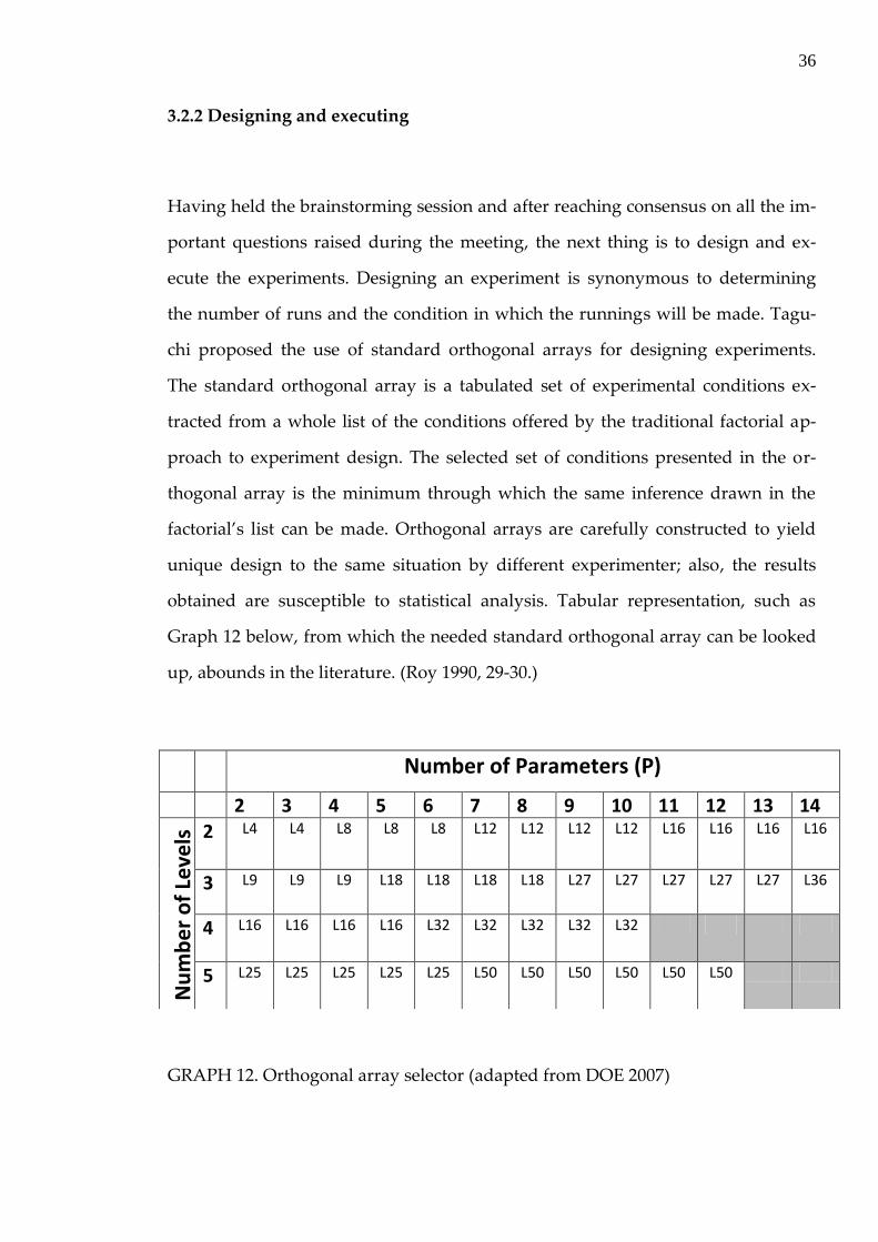
3.2.2 Designing and executing

Having held the brainstorming session and after reaching consensus on all the im-

portant questions raised during the meeting, the next thing is to design and ex-

ecute the experiments. Designing an experiment is synonymous to determining

the number of runs and the condition in which the runnings will be made. Tagu-

chi proposed the use of standard orthogonal arrays for designing experiments.

The standard orthogonal array is a tabulated set of experimental conditions ex-

tracted from a whole list of the conditions offered by the traditional factorial ap-

proach to experiment design. The selected set of conditions presented in the or-

thogonal array is the minimum through which the same inference drawn in the

factorial’s list can be made. Orthogonal arrays are carefully constructed to yield

unique design to the same situation by different experimenter; also, the results

obtained are susceptible to statistical analysis. Tabular representation, such as

Graph 12 below, from which the needed standard orthogonal array can be looked

up, abounds in the literature. (Roy 1990, 29-30.)

GRAPH 12. Orthogonal array selector (adapted from DOE 2007)

Number of Parameters (P)

2 3 4 5 6 7 8 9 10 11 12 13 14

Nu

mb

er

of

Leve

ls 2 L4 L4 L8 L8 L8 L12 L12 L12 L12 L16 L16 L16 L16

3 L9 L9 L9 L18 L18 L18 L18 L27 L27 L27 L27 L27 L36

4 L16 L16 L16 L16 L32 L32 L32 L32 L32

5 L25 L25 L25 L25 L25 L50 L50 L50 L50 L50 L50

37

The number in the names given to the standard orthogonal arrays denotes the

number of test runs required for the specific situation. As an illustration, an expe-

rimenter with four parameters with three levels each at hand will make use of ar-

ray L9 according to Graph 12 above. Presented below is the layout of the condi-

tions embodied by the L9 array.

GRAPH 13. L9 orthogonal array’s layout (adapted from DOE 2007)

With the right array at hand, experiments are designed by mimicking the array.

Once the design is completed, the experiments are run accordingly. Issues regard-

ing execution of the experiments are usually process dependent, for example, the

order in which the runs are made relies on the ease of tuning the parameters’ le-

vels. (Roy 1990, 40-47.)

Experiment P1 P2 P3 P4 1 1 1 1 1

2 1 2 2 2

3 1 3 3 3

4 2 1 2 3

5 2 2 3 1

6 2 3 1 2

7 3 1 3 2

8 3 2 1 3

9 3 3 2 1

38

3.2.3 Analysis of results

The process of analyzing the result from an experiment follows a definite pattern

towards achieving its aims in Taguchi’s philosophy. The aims of the analysis are 1.

to determine the optimum condition, that is, to recognize the set of variable that

yields the result nearest to the target; 2. to estimate the expected performance at

the optimum condition; and 3. to determine the influence of each of the factors on

the results. (Roy 1990, 47-48.)

The analysis process can either make use of the average or signal to noise ratio

values. Apart from the calculation of the averages or the signal to noise ratios, the

analysis procedure is basically the same irrespective of the quantity adopted.

When repetitions of runs are carried out, Taguchi recommends the use of his sig-

nal to noise ratio formulae for the analysis of the results. Otherwise, the conven-

tional averages are made use of. The transformation of the results to signal to

noise(S/N) ratio is made possible with the formula stated below

𝑆/𝑁 = −10 × log10 𝑀𝑆𝐷

Where MSD is the mean squared deviation from the target. Mathematical expres-

sions for the computation of the MSD for the quality characteristics discussed in

earlier heading are as follows:

Smaller the better: 𝑀𝑆𝐷 = 𝑦1

2 + 𝑦22 + 𝑦3

2 + ⋯ 𝑛

Nominal is best: 𝑀𝑆𝐷 = 𝑦1 −𝑚 2 + 𝑦2 −𝑚 2 + ⋯

𝑛

39

Bigger the better: 𝑀𝑆𝐷 = 1

𝑦12 + 1

𝑦22 + 1

𝑦32 + ⋯

𝑛

In these equations, y1, y2, y3 are the results for a particular run at the first, second

and third repetitions respectively; m connotes the target value and n is the number

of repetitions. With the aid of the appropriate formula, the signal to noise ratios

for all the trial conditions in an experiment can be calculated. If the averages were

employed, however, the average value of the n repetitions for every trial condition

would be computed instead. Whichever is the case, either with the signal to noise

ratios or the average values, the average effect of all the studied parameters are

calculated at their respective levels. The average effect of a parameter at a speci-

fied level is accounted for by averaging the results of all the tests containing the

parameter at the level in question. (Roy 1990, 47-98.)

Graphical depiction of average effects of parameters against their respective levels,

for example, as shown in Graph 14 below, is a necessity for the determination of

the optimum state. This graphical illustration is commonly referred to as the main

effects plot. The horizontal line running through the plots is the grand average of

the whole results. This graph makes visible the main effects, the difference be-

tween the average influences of each variable. Thus, preliminary guesses can be

made about the factors influence on the product. The same scale is applied to all

parameter plotting so as to facilitate comparation. The optimum combination is

easily recognized from the graphical illustration. The desired variable combination

depending on whether the quality characteristics are bigger the better, smaller the

better or nominal the best is the factors’ level-set at the top, bottom or nearest to

the target respectively. The optimum conditions in Graph 14 below are A1B3C3D1

40

and A3B1C1D3 for smaller the better and bigger the better sequentially. (Roy 1990,

47-98.)

GRAPH 14. A typical main effects plot.

Having achieved the optimum set of variables, the expected performance can be

estimated with these simple expressions assuming the cases, smaller the better and

bigger the better in Graph 14 above:

𝑌𝑜𝑝𝑡 = 𝐺𝐴 + 𝐴1 − 𝐺𝐴 + 𝐵3 − 𝐺𝐴 + 𝐶3 − 𝐺𝐴 + 𝐷1 − 𝐺𝐴 and

𝑌𝑜𝑝𝑡 = 𝐺𝐴 + 𝐴3 − 𝐺𝐴 + 𝐵1 − 𝐺𝐴 + 𝐶1 − 𝐺𝐴 + 𝐷3 − 𝐺𝐴 where GA is the

grand avergae of all the processed results from the experiment. Further inquiry

into the factors’ influence on the products can be made with the famous analysis

of variance (ANOVA). It should be noted that factors contributions calculated

with the ANOVA technique are relative to one another. The result of the ANOVA

A1

A2

A3

B1

B2

B3

C1C2

C3

D1

D2

D3

5

6

7

8

9

10

11

12

13

14

Ave

rage

Eff

ect

S/N Main Effects

41

calculation is usually presented in a table showing a number of calculated quanti-

ties and the relative contribution of each factor in percent. Table 1 below shows an

ANOVA table with all its presented quantities usually calculated. (Roy 1990, 47-

98.)

TABLE 1. An ANOVA table

COL-

UMN

FAC-

TORS

DEGREE

OF

FREE-

DOM

SUM OF

SQUAR

ES

VA-

RIANCE

VA-

RIANCE

RATIO

PERCENT

CONTRIBU-

TION

1 Factor1 -- -- -- -- --

2 Factor2 -- -- -- -- --

3 Factor3 -- -- -- -- --

Oth-

ers/Error

-- -- -- -- --

Total -- -- 100

The quantities shown in Table 1 above are briefly explained below with the ap-

propriate formula for their evaluation when necessary:

Degree of freedom: The degree of freedom, DOF, is one less than the num-

ber of levels of a variable. Similarly for an array, the DOF is one less than its

number of levels or rows it contains. Thus a parameter with three different

levels has two as its DOF, whereas an L9 array displayed in Graph 2 has

eight as its DOF. However, the DOF for a set of experimental result is calcu-

lated as follows:

DOF = number of results - 1;

42

and DOF = number of results *number of repetition – 1, when there is repe-

tition. The first expression is always the case when S/N is used in the analy-

sis process. Lastly, the DOF for error variance is that of the total experiment

set minus that of each of the variables in the experiment.

Sum of squares: The total sum of squares, ST, is calculated by summing the

squares of the results of the experiment and subtracting the correction fac-

tor, CF, from it. The equations are presented below

𝑆𝑇 = 𝑦2 − 𝐶𝐹 𝑤𝑕𝑒𝑟𝑒 𝐶𝐹 = 𝑦 2

𝑛

The factors’ sum of squares can be calculated as illustrated below using a

factor A with two levels as an example

𝑆𝐴 =𝐴1

2

𝑁𝐴1 +

𝐴22

𝑁𝐴2 − 𝐶𝐹 where A1 and A2 are the sum of the results in

which level1 and level2 values of the factor A are present; and NA1 and NA2

are their respective number of experiments in which factor A’s level 1 and 2

participated or the number of results summed up to get A1 and A2. Just like

with the DOF, sum of squares for error is the total sum of squares minus

those of the factors. The estimation of the other error parameters takes the

same approach.

Variance: The term variance is defined as the ratio of the sum of squares to

the DOF. For example, factor A’s variance can be calculated as 𝑉𝐴 =

𝑆𝐴𝐷𝑂𝐹𝐴 .

Variance ratio: This is the ratio of the variance of any factor to that of the er-

ror. When the error’s variance is zero, the variance ratios are all rendered

indeterminate. In such a case, the error’s variance can be combined with

43

that of any factor whose value is relatively insignificant. Say a variable B

possesses small variance, then that of the error can be reestimated as thus;

𝑉𝑒𝑟𝑟𝑜𝑟 =𝑆𝐵 + 𝑆𝑒𝑟𝑟𝑜𝑟

𝐷𝑂𝐹𝐵 + 𝐷𝑂𝐹𝑒𝑟𝑟𝑜𝑟 . The merging of any factor’s variance

with that of the error is termed pooling. Afterwards, the variance ratios can

be calculated and the sum of squares are also adjusted as follows; 𝑆𝐴′ = 𝑆𝐴 −

𝑉𝑒𝑟𝑟𝑜𝑟 × 𝐷𝑂𝐹𝐴 . The newly calculated sums of squares- pure sum of

squares- are used for the contribution calculation.

Percentage contribution: The ratio of the sum of squares of a factor to that

of the total result multiplied by hundred is called the factor’s contribution

in percent. The percentage contribution or influence of the factors on the re-

sult is that goal of the ANOVA calculation

𝑃𝐴 =𝑆𝐴

𝑆𝑇 × 100

(Roy 1990, 47-98 & 101-155.)

3.2.4 Confirmatory test

Running a confirmatory test is usually the last stage in the process of experiment-

ing following the Taguchi’s approach. As a continuation from the results analysis,

the optimum result, Yopt, predicted at the determined optimum condition must be

verified. This is actually one of the beauties of the Taguchi’s method. In order to

validate the prediction, new experiment trials, whose results will be juxtaposed

with the one arrived at by equation, have to be made. (Roy 1990, 31; Statsoft 2010.)

44

The comparation of the two results should show a reasonable agreement; other-

wise possible interaction between variables might have prompted a disagreement.

The decision of whether or not to study interactions is made in the brainstorming

stage. If an interaction is left out when it is significant, it will tell on the final re-

sults; this further emphasizes the need for an elaborate brainstorming session.

45

4 EXPERIMENTATION

The pilot scale CO2-MEA absorption-desorption unit installed in the laboratory of

Central Ostrobothnia University of Applied Sciences was observed to accumulate

CO2 as it was being run. It was also observed that this was as a result of the ineffi-

ciency of the desorber which constantly floods. Thus, this experiment is aimed at

optimizing the CO2 removal or regeneration of the washing liquid in the stripper.

This experimentation will follow closely the Taguchi approach, and thus, the pro-

posed four-stage process for the determination of the optimum condition would

be strictly adhered to. A detailed description of the experiment equipment and

procedure will be offered in the subsequent subheadings.

4.1 Equipment description

The CO2-MEA absorption-desorption unit utilized in this experiment, depicted in

Graph 15, has the following features: an absorber of diameter 100mm and a desor-

ber of diameter 80mm both made of transparent glass and packed with 10mm Ra-

schig ring; a shell and tube heat exchanger positioned in between the packed col-

umns for allowing heat exchange between the two columns feed; two storage

tanks with a centrifugal pump each for the circulation of the washing liquid; a

plate heat exchanger through which hot steam’s flow energizes the stripper’s con-

tent to release CO2 and steam; a heating coil for preheating the stripper’s feed, and

a metallic cylinder which contains CO2 gas.

46

GRAPH 15. The CO2-MEA absorption-desorption unit

The control and measurement facilities of the parts of the unit mentioned are pin-

pointed below:

The pumps are controlled from the user interface on a desktop computer.

The pumps run based on the set flow rate and they also work in such a way

that the liquid levels in the tanks are always leveled. The tank level can be

seen from the user interface.

The carbon dioxide flow can be adjusted with the knob on the cylinder

while the airflow is controlled with a valve linked with the pipeline supply-

ing air to the laboratory. The two streams are mixed on their way to the ab-

sorber where an online sensor has been installed to detect the CO2 content.

47

The preheater is the easiest to control. It has three power levels which can

be chosen with a switch.

The steam flow can be controlled by turning a restrictor either clockwise or

anticlockwise. As the restrictor is being turned, the corresponding pressure

can be checked on a pressure meter installed along the steam’s passage.

Lastly, several online sensors were installed at different points within the

columns to measure pressure drops and temperatures.

4.2 Experimental procedure

In line with the principles of parameter design, the experiment started with the

brainstorming session which had five participants: the project supervisor, labora-

tory assistance, and three students whose theses are related to the subject matter.

The aim of the meeting, which was to optimize the CO2 removal in the desorber,

was stated and then exchange of ideas began on how to achieve the goal. In about

an hour of discussion, concessions were reached as regards the factors affecting

the functionality of the stripper column to be considered in the experiment, the

levels of variables to be tested; the performance parameter, and the quality charac-

teristics. The agreement reached is summarize in Table 2 below.

TABLE 2. Agreed condition for the MEA regenerating process optimization

Variables Level 1 Level 2 Level 3

CO2 load (%) 10 15 20

Liquid flow (l/min) 2.5 3.0 3.5

48

Steam’s pressure (bar) 0.20 0.25 0.30

Preheater’s power (kW) 2 4 6

Performance parameter : CO2 removal in the stripper

Quality characteristics : Bigger the better

Following the accord on the variables and levels to be studied, a L9 array was

used to design the experiment. Three repetitions were made each so as to use the

signal to noise ratio in the analysis. Table 6 below shows the experiment condi-

tions as deduced with the L9 array.

TABLE 3. Experimental condition layout for MEA regeneration optimization

Trial

Number

CO2 load

(%)

Liquid flow

(l/min)

Steam’s

pressure

(bar)

Preheater’s

power

(kW)

CO2 re-

moval

1 10 2.5 0.20 2

2 10 3.0 0.25 4

3 10 3.5 0.30 6

4 15 2.5 0.25 6

5 15 3.0 0.30 2

6 15 3.5 0.20 4

7 20 2.5 0.30 4

8 20 3.0 0.20 6

9 20 3.5 0.25 2

Before the experiment plan displayed in Table 3 was executed, the absorption-

desorption unit was drained of its old washing liquid and thoroughly rinsed with

deionized water to remove any fouling from the packing surface. Afterwards, sev-

49

eral liters of 1M MEA were prepared into the two storage tanks from which they

were been pumped into the absorber and the desorber continuously until the

packings became adequately wet.

Having gotten the packings wet, the variables were tuned to the appropriate con-

ditions stated in the experiment plan. Time interval of about thirty minutes was

allowed in between trials to enable the system stabilize; however, the CO2 load

varies slightly in the course of the experiments. Samples of the washing liquid en-

tering and leaving the stripper were taken for CO2 analysis. Additionally, pressure

drop and temperature measurement around the columns were also recorded for

all the trials.

The CO2 content of the amine solutions was separated and measured with the

simple apparatus shown in Graph 16. As seen from Graph 16, the burette and the

funnel to some extent contain the sealing liquid—a mixture of distill water, so-

dium sulphate salt and concentrated sulphuric acid—used to trap the released

CO2 from the two sided tube. In the glass tube on the other hand, 2ml of the MEA

solution and 5ml of a 50% by weight phosphoric acid solution on the either sides

were mixed for each trial’s sample. The changes in the level of the burette’s con-

tent were noted as the volume of CO2 released.

50

GRAPH 16. CO2 analysing equipment

The recorded data for the experimental runs and the samples analysis are pre-

sented in the next chapter.

51

5 DATA AND CALCULATIONS

In continuation with the CO2 removal optimization experiment, the data collected

from the experiments described in the previous chapter were utilized for some

calculations. Shown below in Table 4 are the values of the CO2 removal estimated

from the collected data.

TABLE 4. CO2 removal for the experiment trials

Trial Num-

bers

CO2 removal per 2ml MEA solution (ml)

1st Run 2nd Run 3rd Run

1 2.35 2.3 2.25

2 1.55 3.02 2.7

3 1.15 4.05 3.75

4 7.95 5.85 7.55

5 1.9 1.35 2.95

6 2.37 2.5 2.15

7 4.95 7.55 9.3

8 4.4 7.07 5.7

9 1.35 1.9 2.1

52

With these data, the necessary calculations were made to determine the optimum

CO2 removal condition, the expected CO2 removal at this condition and the contri-

bution of each parameter to the results.

To start with, the performance parameter values (CO2 removal) were converted to

signal to noise ratio using the equation for bigger the better. The procedure is dis-

played below with the first trial results from Table 4.

𝑆/𝑁 = −10 × log10 1

𝑦12 + 1

𝑦22 + 1

𝑦32

𝑛

𝑆/𝑁 = −10 × log10 1

2.352 + 12.32 + 1

2.252

3 = 7.23

The same equation was used for the remaining trials to arrive at the values ga-

thered in Table 5.

TABLE 5. Signal to noise ratios for experiment trials

Trial

Number

CO2 load

(%): A

Liquid flow

(l/min): B

Steam’s

pressure

(bar): C

Preheater’s

power

(kW): D

Signal to

Noise

Ratio

1 1 1 1 1 7.23

2 1 2 2 2 6.56

3 1 3 3 3 5.29

4 2 1 2 3 16.81

5 2 2 3 1 5.04

53

6 2 3 1 2 7.33

7 3 1 3 2 16.33

8 3 2 1 3 14.67

9 3 3 2 1 4.55

With the S/N values, the average effects of all the parameters were calculated at

their stated levels. In the case of variable A (CO2 load) ; its average performance at

level1 is the average of all the S/N ratio values that include parameter A at level1,

therefore:

𝐴1 = 7.23 + 6.56 + 5.293 = 6.36

Other average effects were calculated similarly, and then used to chart the so

called main effect graph from which the sought optimum condition was evident.

TABLE 6. Average effects of parameters

Average Effects

Variables Level 1 Level 2 Level 3

CO2 load (%): A 6.357397 9.725596 11.84704

Liquid flow

(l/min): B 13.45409 8.75315 5.722795

Steam’s pressure

(bar): C 9.743435 9.30378 8.882821

Preheater’s power

(kW): D 5.605564 10.07145 12.25302

54

GRAPH 17. Main effect plots for the four parameters

The optimum condition was chosen as the set of variables level highest on the

main effect plots. This set of condition is A3 (20% CO2 load), B1 (2.5 l/min liquid

flow), C1 (0.2bar steam’s pressure) and D3 (6kW preheater’s power). Following

this, the grand average (GA) signal to noise ratio was estimated to be 9.31.

The expected signal to noise ratio and CO2 removal at the optimum condition

were calculated with these expressions:

𝑆/𝑁𝑜𝑝𝑡 = 𝐺𝐴 + 𝐴1 − 𝐺𝐴 + 𝐵3 − 𝐺𝐴 + 𝐶3 − 𝐺𝐴 + 𝐷1 − 𝐺𝐴

A1

A2

A3

B1

B2

B3

C1C2

C3

D1

D2

D3

5

6

7

8

9

10

11

12

13

14

0 2 4 6 8 10 12 14 16

Re

spo

nce

s (

Sign

al t

o n

ois

e r

atio

val

ue

s)

Variables

55

and ∆𝐶𝑂2,𝑜𝑝𝑡 = 10(𝑆/𝑁𝑜𝑝𝑡 )

10 . The expressions yielded 19.37 and 9.3ml for the ex-

pected optimum S/N ratio and the change in carbon dioxide removal respectively.

Lastly, analysis of variance (ANOVA) was performed on the data to detect the fac-

tors respective influence on the results. In the first analysis, the error factor has an

infinitesimal variance. Also, it was discovered that the reboiling steam pressure

influence is insignificant; thus, the analysis was repeated with factor C being

pooled. The outcome of the second ANOVA calculation is shown in Table 7 below.

TABLE 7. ANOVA calculation with pooling

Co

lum

n Factors Degree

of free-

dom

Sum of

squares

Variance Variance

ratio

Pure

sum of

squares

Percent

contri-

bution

1 CO2 load

(%): A

1 45.98 45.98 206.91 45.76 22.10

2 Liquid

flow

(l/min): B

1 91.05 91.06 409.73 90.83 43.87

3 Steam’s

pressure

(bar): C

pooled pooled pooled pooled pooled pooled

4 Prehea-

ter’s pow-

er (kW): D

1 68.89 68.89 310.00 68.67 33.17

Oth-

ers/Err

or

5 1.11 0.22 0.86

Total 8 207.04 100

56

From the last column in Table 7, it can be clearly seen that variables A, B and D

have significant influence on the experiment outcome. This singular reason calls

for a close watch on the variation of these variables as a slight deviation from their

fixed point can greatly affect the result.

In order to validate the claims made with the calculated optimum condition, three

runs were made at the proposed condition. The results from these runs are pre-

sented in Table 8 below.

TABLE 8. Confirmatory tests results

Trial Condition ∆CO2 per 2ml MEA solution (ml)

1st Run 2nd Run 3rd Run

A3 (20% CO2 load), B1 (2.5 l/min liquid

flow), C1 (0.2bar steam’s pressure) and

D3 (6kW preheater’s power)

5.00 6.20 9.80

The carbon dioxide released per 2ml MEA solution from the confirmatory tests

has an average of 7.00ml. This value is about 25% less than the one calculated from

the stated optimum condition. A possible reason for this is the presence of interac-

tion between some of the variables investigated or the inability of the system to

stabilize as the result of constant variation of variables in the course of the trial.

The trend of the figures in Table 8 also seems to suggest that the unit is not stabi-

lized before washing liquid samples are being taken.

57

6 DISCUSSION

Absorption-desorption units are widely used for the purpose of carbon dioxide

sequestering. The overall efficiency of these units can be tied to a number of fac-

tors amongst which is the effective washing liquid regeneration. This thesis’ goals

are to investigate the variables affecting CO2 stripping, to optimize the stripping

process and lastly to give recommendations on how to improve the CO2 stripping

capacity of the CO2-MEA absorption-desorption unit whose desorber is unable to

effectively regenerate its washing liquid, MEA.

In the light of these tasks, thorough research was made to elucidate the intricacies

surrounding the subject matter, and also to make clear the recognition of the fac-

tors affecting CO2 stripping. Afterwards, the Taguchi method of experimentation

was employed to optimize the regeneration process.

According to literature, the following factors were found to affect the stripping

ability the desorber: inlet carbon load, liquid inlet temperature; the reboiling heat,

liquid flow rate; packing type, washing liquid’s nature and characteristics; height

of the packing, and the column diameter. The first four of the listed factors were

studied in the experiment to determine their optimum combinations, as they are

readily tunable. Affecting other factors suggests retrofitting the system.

The sought optimum combination of the studied variables was found to be 20%

CO2 load, 2.5 l/min washing liquid flow, 0.2bar steam’s pressure and 6kW prehea-

58

ter’s power after running twenty-seven straight experiments at nine different con-

ditions. Theoretical estimation of carbon dioxide removal at this condition yields

9.3ml; however, the confirmatory test gave 7.0ml CO2 removal. Carbon load, liq-

uid flow and preheater’s power were found to significantly influence the stripping

process.

The notable difference between the calculated and the empirically determined CO2

removal calls for further investigation to better achieve the optimization. This

time, possible interactions within the variables should be involved in the study.

Additionally, a better control system should be built around the three variables

said to be substantially influencing the results.

Likewise, the capacity of the desorber can be extended by effecting the two

changes discussed below:

Usage of better packing: Raschig rings, which are currently utilized in the

stripper, also in the absorber, are the oldest form of packings known. There

are tenths of better random packing types with better interfacial area avail-

able for mass transfer. However, considering that the scrubber is more in

size as compared to the stripper, the capacity extension that can be ren-

dered by another random packing might be immaterial. Thus, a structural

packing, known for its low pressure drop, is suggested.

Washing solvent situation: A rough estimation of the percent CO2 being

handled in the system indicates a value above which chemically absorbing

solvents are known to perform well. However, an examination of the condi-

tion of state (pressure and temperature condition) in the system favors the

chemically working liquid. A change to a physically working solvent would

59

required higher pressure which the all-glass equipment might not be able

withstand. However, this change will save cost as less heating will be re-

quired from the reboiler and at the same time better the regeneration

process.

In conclusion, in order to operate this equipment with better washing liquid rege-

neration, the four-variable optimizing condition stated above must be adhered to.

However, improving the capacity of the desorber involves the retrofitting actions

stated above as well.

REFERENCES

CO2CRC 2010. CO2 capture/separation technologies. Available:

http://www.co2crc.com.au/aboutccs/cap_absorption.html. Accessed 10 May 2010 .

DOE 2007. Design of experiment via Taguchi methods: Orthogonal arrays. Avail-

able:

http://controls.engin.umich.edu/wiki/index.php/Design_of_experiments_via_tagu

chi_methods:_orthogonal_arrays. Accessed 13 March 2010.

Green, D., W. and Perry, H., R. 2008. Perry’s Chemical Engineers’ Handbook.

Eighth Edition. New York: McGraw-Hill, USA.

Koonaphapdeelert, S., Wu, Z. and Li, K. 2009. Carbon dioxide stripping in a ce-

ramic hollow fibre membrane contactors. Chemical Engineering Science 64, 1-8.

Li, J. and Chen, B. 2005. Review of CO2 absorption using chemical solvents in hol-

low fibre membrane contactors. Separation and Purification Technology 41, 109-

122.

Longo, G., A. and Gasparella, A. 2006. Experimental analysis on desiccant regen-

eration in a packed column with structured and random packing. Solar Energy 83,

511-521.

McCabe, W., L., Smith, J., C. and Harriott, P. 2005. Unit Operations of Chemical

Engineering. Seventh Edition. New York: McGraw-Hill, USA.

Reference 2010. Experiment. Available:

http://www.reference.com/browse/experiment. Accessed 15 March 2010.

Roy, R. 1990. A primer on the Taguchi method. New York: Van Nostrand Rein-

hold.

Saint-Gobain 2001. Packed tower internal guide. Available:

http://www.coastalchem.com/PDFs/Norton/Packed%20Tower%20Internals%20Gu

ide.pdf. Accessed 15 March 2010.

Seader, J., D. and Henley, E., J. 2004. Separation process principles.( 2nd Edition)

NJ: John Wiley & Sons, Inc.

Statsoft 2010. Experimental design. Available:

http://www.statsoft.com/textbook/experimental-design/?button=1. Accessed 7

April 2010.

Strelzoff, S. 1980. Choosing the optimum CO2-removal system. Separation Tech-

nology 2: Gas/Liquid/Solid Systems. New York: McGraw Hill Publication Compa-

ny.

Sulzer Chemtech 2010. Internals for packed columns. Available:

http://www.sulzerchemtech.com. Accessed 10 April 2010.

Zenz, F., A. 1980. Designing gas-absorption tower. Separation Technology 2:

Gas/Liquid/Solid Systems. New York: McGraw Hill Publication Company.

APPENDIX 1/1

Raw data collected from the experiments were presented below.

First run

Experi-

peri-

ment

Num-

ber

Tga

s,

in

deg

, C

Tga

s,

out

deg

, C

Tli

q,

in

de

g,

C

Tli

q,

out

de

g,

C

Tliq,

in(Strip

per)

deg, C

Strip

per

PD

mbar

Ab-

sorber

PD

mbar

CO

2

loa

d

in

%

CO

2

loa

d

out

%

CO

2

in

ml

CO

2

out

ml

1 16.0 12.

6

10.

7

9.5 55.1 1.8 3.6 10.

05

6.7

0

20 17.

65

2 16.7 10.

0

10.

0

10.

1

64.9 2.2 4.0 10.

18

7.3 19.

85

18.

3

3 16.5 10.

4

11.

0

11.

2

71.9 2.7 4.3 9.4

8

7.5

3

19.

6

18.

45

4 16.6 12.

2

9.6 11.

1

85.7 50.2 4.9 14.

9

9.1

2

20.

05

12.

1

5 16.7 10.

8

9.8 11.

6

54.9 2.7 5.4 14.

26

10.

95

21.

0

19.

1

6 14.7 10.

9

10.

9

11.

0

62.5 3.1 7.2 15.

60

11.

97

22.

9

20.

53

7 7.9 9.2 10.

5

11.

8

70.7 3.2 5.2 20.

66

9.0

6

23.

65

18.

7

8 11.8 10.

2

12.

1

13.

9

80.3 5.9 19.

66

12.

62

22.

05

17.

65

9 11.9 10.

6

13.

2

13.

7

54.7 7.8 19.

80

14.

32

23.

35

22.

0

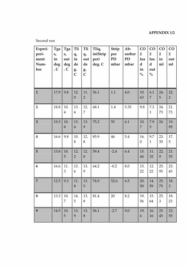
APPENDIX 1/2

Second run

Experi-

peri-

ment

Num-

ber

Tga

s,

in

deg

. C

Tga

s,

out

deg

. C

Tli

q,

in

de

g.

C

Tli

q,

out

de

g.

C

Tliq,

in(Strip

per)

deg. C

Strip

per

PD

mbar

Ab-

sorber

PD

mbar

CO

2

loa

d

in

%

CO

2

loa

d

out

%

CO

2

in

ml

CO

2

out

ml

1 17.9 9.8 12.

0

11.

2

56.1 1.1 4.0 10.

63

6.1

7

24.

5

22.

2

2 18.8 10.

4

13.

4

12.

7

68.1 1.4 5.35 9.8 7.3

1

24.

75

21.

73

3 19.3 10.

8

13.

4

13.

9

75.2 55 6.1 10.

7

7.9

5

24 19.

95

4 16.6 9.8 10.

8

12.

8

85.9 46 5.4 16.

0

9.7

1

23.

35

17.

5

5 15.8 10.

5

12.

2

12.

8

59.4 -2.4 6.4 15.

44

11.

32

22.

9

21.

55

6 16.6 11.

3

13.

6

13.

9

64.2 -0.2 8.0 15.

22

12.

22

25.

95

23.

45

7 12.5 9.3 11.

8

13.

5

74.9 52.6 6.5 20.

50

14.

59

25.

75

18.

2

8 13.3 10.

7

14.

5

13.

8

81.4 20 8.2 19.

56

15.

64

25.

3

18.

23

9 14.5 10.

5

13.

9

13.

8

56.1 -2.7 9.0 19.

6

16.

16

25.

45

23.

55

APPENDIX 1/3

Third run

Experi-

peri-

ment

Num-

ber

Tga

s,

in

deg

. C

Tga

s,

out

deg

. C

Tli

q,

in

de

g.

C

Tli

q,

out

de

g.

C

Tliq,

in(Strip

per)

deg, C

Strip

per

PD

mbar

Ab-

sorber

PD

mbar

CO

2

loa

d

in

%

CO

2

loa

d

out

%

CO

2

in

ml

CO

2

out

ml

1 15.5 8.7 12.

0

11.

9

45.31 2.1 3.9 10.

0

6.0

4

25.

5

23.

25

2 15.9 8.6 12.

9

13.

3

67.8 1.4 4.9 10.

2

7.0

3

25.

45

22.

75

3 17.7 10.

2

12.

9

14.

5

76.0 58.9 8.8 10.

15

8.7

9

25.

25

21.

5

4 15.1 9.2 11.

2

13.

2

86.4 50.2 6.1 15.

04

10.

64

25.

9

18.

35

5 12.9 10.

1

13.

8

12.

8

55.7 1.8 5.9 15.

50

9.8

1

27.

95

25.

0

6 13.8 11.

2

14.

8

14.

2

62.2 1.6 7.4 15.

20

11.

35

28.

35

26.

2

7 10.9 9.7 12.

2

13.

1

70.2 55.2 7.3 20.

20

15.

15

30.

05

20.

75

8 10.8 10.

3

13.

8

14.

7

79.2 57.7 8.2 20.

05

16.

04

28.

2

22.

5

9 9.7 10.

9

15.

4

14.

5

51.7 1.2 9.3 20.

50

15.

06

29.

9

27.

8

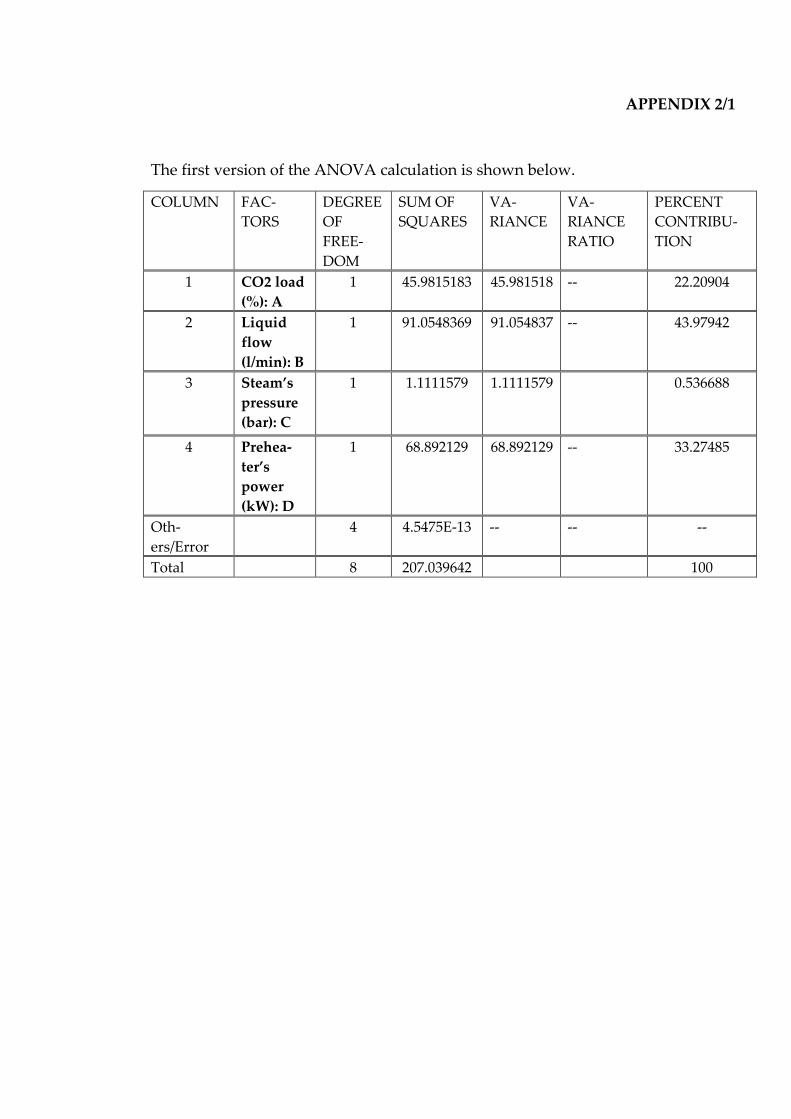
APPENDIX 2/1

The first version of the ANOVA calculation is shown below.

COLUMN FAC-

TORS

DEGREE

OF

FREE-

DOM

SUM OF

SQUARES

VA-

RIANCE

VA-

RIANCE

RATIO

PERCENT

CONTRIBU-

TION

1 CO2 load

(%): A

1 45.9815183 45.981518 -- 22.20904

2 Liquid

flow

(l/min): B

1 91.0548369 91.054837 -- 43.97942

3 Steam’s

pressure

(bar): C

1 1.1111579 1.1111579 0.536688

4 Prehea-

ter’s

power

(kW): D

1 68.892129 68.892129 -- 33.27485

Oth-

ers/Error

4 4.5475E-13 -- -- --

Total 8 207.039642 100

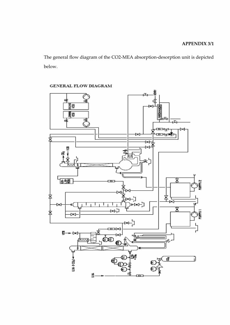
APPENDIX 3/1

The general flow diagram of the CO2-MEA absorption-desorption unit is depicted

below.