optimization of coagulant and coagulant aid in …

Guiming Su

OPTIMIZATION OF COAGULANT AND COAGULANT AID IN

WASTEWATER TREATMENT

Thesis

CENTRIA UNIVERSITY OF APPLIED SCIENCES

Environmental Chemistry and Technology

April 2019

ABSTRACT

Centria University

of Applied Sciences

Date

April 2018

Author

Guiming Su

Degree programme

Environmental Chemistry and Technology

Name of thesis

OPTIMIZATION OF THE COAGULANT AND COAGULANT AID IN THE WASTEWATER

TEATMENT

Instructor

Anu-Sisko Perttunen, JunJun Shi

Pages

50 + 4

Supervisor

Jana Holm

With the expanding urbanization, more municipal wastewater is produced by citizens, which requires

more efficient wastewater treatment to meet the demand of stringent legislation.

This thesis aimed to enhance the functions of coagulation and flocculation in the wastewater treatment

process, which can lead to the optimal dosing of chemical reagent and the lower chemical residual in

the post-treated wastewater. The project was approached by reviewing relevant literature and conduct-

ing experiments. The literature showed the current approach of the coagulation and flocculation in the

wastewater treatment as well as their functional principles. In the experiment part, the parameters of

turbidity and the residual of the chemical reagent were measured. During the procedures, Jar Test was

implemented, and the optimal dose of the coagulant and the best operational pH were determined. Other

factors such as the mixing intensity, mixing time were discussed in this thesis.

Key words

Coagulation, Flocculation, Jar test, Turbidity, Municipal Wastewater.

ACKNOWLEDGEMENTS

I would like to express my sincere gratitude to my supervisor Jana Holm and laboratory instructor Anu-

Sisko Perttunen who gave me advice, invaluable assistance, and guidance through the whole process of

this thesis.

I would like to say thanks to engineer Ville Sydänmetsä and the staff from Hopeakivenlahti wastewater

treatment plant, who gave me a lot information of the wastewater plant and helped me take sample.

I want to say thank you to Eelis Kähkönen from Kemira Oyj, who provided the information of their

chemical products.

I want to appreciate Anna Kirveslahti, Kari Jääskeläinen and other researchers from the Centria’s R&D

department, who gave me a lot of help and instruction of operating machines.

I would like to say thanks to my teacher JunJun Shi from Foshan University, my classmates Markus

Perä and Tomas Chacon who gave me invaluable support during the process of thesis.

Furthermore, I have almost finished one-year study of double degree program in Finland. I would like

to express my appreciation to my family, the teachers from both Centria University of Applied Sciences

and Foshan University who dedicated themselves to promote the program, and the classmates who

helped me in the past one year.

CONCEPT DEFINITIONS

BOD Biochemical oxygen demand

COD Chemical oxygen demand

TS Total solid

TSS Total suspended solid

TVS Total volatile solid

NOM Nature organic matter

WWTP Wastewater treatment plant

EDL Electric double layer

RPM Rotations per minute

AAS Atomic absorption spectroscopy

ABSTRACT

ACKNOWLEDGEMENTS

CONCEPT DEFINITIONS

CONTENTS

1 INTRODUCTION ................................................................................................................................ 1

2 LITERATURE REWIEW .................................................................................................................. 3

2.1 Wastewater ..................................................................................................................................... 3 2.1.1 Industrial wastewater .......................................................................................................... 3 2.1.2 Domestic wastewater ............................................................................................................ 6 2.1.3 Characteristics of the domestic wastewater ....................................................................... 7 2.1.4 Contaminants in wastewater ............................................................................................... 7

2.1.5 Wastewater plant ................................................................................................................. 8

2.1.6 Main processes of treatment ............................................................................................... 8 2.2 Turbidity of wastewater .............................................................................................................. 10

2.3 Coagulation and flocculation ...................................................................................................... 10 2.4 Stability of particles in water ...................................................................................................... 11 2.5 Principles of coagulation and flocculation ................................................................................. 13

2.6 Coagulant and flocculant ............................................................................................................. 14 2.6.1 Coagulant ............................................................................................................................ 15 2.6.2 Flocculant ............................................................................................................................ 16

2.7 Jar test ........................................................................................................................................... 17 2.7.1 Parameters concerned in Jar Test .................................................................................... 18

2.7.2 Configuration of Jar Test .................................................................................................. 19

3 EXPERIMENT .................................................................................................................................. 21

3.1 Basic chemical reagents and source of wastewater ................................................................... 21 3.2 Main equipment ........................................................................................................................... 21

3.3 Basic calculation ........................................................................................................................... 23 3.4 Basic characteristic of raw wastewater ...................................................................................... 24

3.5 Optimal dose and dosing conditions of coagulant ..................................................................... 25

3.5.1 Optimal dose of coagulant ................................................................................................. 25 3.5.2 Optimal dosing pH ............................................................................................................. 27

3.5.3 Re-determination of the optimal coagulant dose ............................................................. 28 3.6 Effect of initial mixing intensity .................................................................................................. 29 3.7 Effect of flocculation mixing intensity ........................................................................................ 29

3.8 Effect of flocculation mixing time ............................................................................................... 30

4 RESULTS AND DISCUSSION ........................................................................................................ 32

4.1 Basic characteristic of raw wastewater ...................................................................................... 32

4.2 Optimal dose and dosing condition of coagulant ...................................................................... 32 4.2.1 Optimal dose of coagulant ................................................................................................. 33 4.2.2 Optimal dosing pH ............................................................................................................. 34 4.2.3 Re-determination of the optimal dose of coagulant ........................................................ 35

4.3 Effect of the initial mixing intensity ........................................................................................... 36

4.4 Effect of the flocculation mixing intensity ................................................................................. 37 4.5 Effect of the flocculation mixing time ......................................................................................... 39

5 CONCLUSIONS ................................................................................................................................ 41

REFERENCES ...................................................................................................................................... 42

APPENDICES

APPENDIX 1: Sampling sites in Hopeakivenlahti WWTP

APPENDIX 2: AAS calibration curve and method

APPENDIX 3: PIX-105 coagulant data sheet

APPENDIX 4: Optimal operation of PIX-105 provided by Kemira

GRAPHS

GRAPH 1. Optimal dose of coagulant .................................................................................................... 34

GRAPH 2. Optimal dosing pH ............................................................................................................... 35

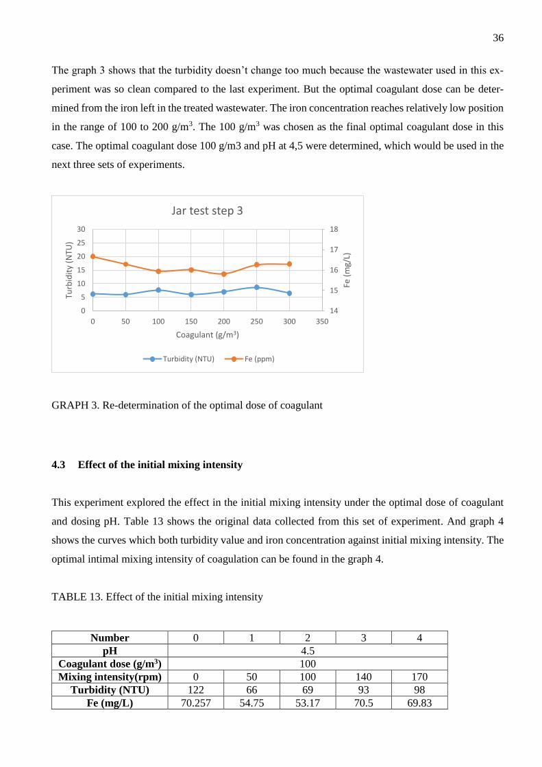
GRAPH 3. Re-determination of the optimal dose of coagulant ............................................................. 36

GRAPH 4. Effect of the initial mixing intensity ..................................................................................... 37

GRAPH 5. Effect of flocculation mixing intensity ................................................................................. 38

GRAPH 6. Effect of the flocculation mixing time .................................................................................. 40

FIGURES

FIGURE 1.Industrial wastewater classification (adapted from Chandrappa & Diganta 2014) ................ 4

FIGURE 2. Classification of dissolved solids based on biodegradability (adapted from Chandrappa &

Diganta 2014) ............................................................................................................................................ 4

FIGURE 3.Basic flowchart of wastewater treatment plant (adapted from Gray 2010) ............................ 9

FIGURE 4.Flowchart of coagulant dosing and coagulant aid in Hopeakivenlahti WWTP (adapted from

Sydänmetsä 2018) ................................................................................................................................... 10

FIGURE 5.Typical wastewater process employing coagulation with conventional treatment, direct

filtration or contact filtration (adapted from Trussell & John 2012) ...................................................... 11

FIGURE 6. Structure of the electrical double layer (adapted from Trussell &John 2012, 145) ............ 12

FIGURE 7. Physical models of coagulation-flocculation process (adapted from Hanhui, Xiaoqi &

Xuehui 2004)........................................................................................................................................... 14

FIGURE 8. Solubility diagram for (a) Al(III) and (b) Fe(III) at 25C (adapted from Trussell &John et

al. 2012,152.) .......................................................................................................................................... 16

FIGURE 9. Jar test unit (adapted from AWWA Staff et al, 2010, 25.) .................................................. 20

FIGURE 10. Rotational stirrer(left), paddle (middle) and Turbidity meter (right) ................................ 22

FIGURE 11. Syringe and filter disk (left) and AAS analyzer (right) ..................................................... 22

FIGURE 12. Raw wastewater from the first sampling site. .................................................................... 25

FIGURE 13. Coagulation (left) and flocculation (right) ......................................................................... 26

FIGURE 14. Treated wastewater ............................................................................................................ 33

FIGURE 15. Small pieces of flocs suspended in water .......................................................................... 39

TABLES

TABLE 1. Source of chemicals from various industries (adapted from Chandrappa & Diganta et al.

2014) ......................................................................................................................................................... 5

TABLE 2. Typical organic coagulant aids used in the water treatment (adapted from John 2012, 575.)

................................................................................................................................................................. 17

TABLE 2. Determination of optimal coagulant dose ............................................................................. 26

TABLE 4. Determination of optimal pH ................................................................................................ 27

TABLE 5. Re-determination of the optimal coagulant dose .................................................................. 28

TABLE 6. Effect of initial mixing intensity ........................................................................................... 29

TABLE 7. Effect of flocculation mixing intensity ................................................................................. 30

TABLE 9. Characteristics of wastewater ................................................................................................ 32

TABLE 10. Optimal dose of coagulant .................................................................................................. 33

TBALE 11. Optimal dosing pH .............................................................................................................. 34

TABLE 12. Re-determination of the optimal dose of coagulant ............................................................ 35

TABLE 13. Effect of the initial mixing intensity ................................................................................... 36

TABLE 14. Effect of the flocculation mixing intensity .......................................................................... 38

TABLE 15. Effect of the flocculation mixing time ................................................................................ 39

1

1 INTRODUCTION

Water is not a commercial product like any other but, rather, a heritage which must be protected, de-

fended and treated as such. It is one of the most important resources for humans and other creatures on

the planet. There is no doubt that life originates from the water. As we all know that approximately 71%

of the earth’s surface is covered with the water, which seems to show the evidence that we have plenty

of water to meet the demand of water. But the truth is that fresh water is limited for human.

With the development of economy and technology, urbanization speeds up all around the world, which

causes that high demand of the fresh water as well as the large amount of wastewater produced by the

households and industrial plants. Nowadays, a lot of countries are becoming more conscious about the

wastewater treatment issues than ever before because countless environmental incidents show that it is

time to solve the problems between humans and environment, which aims to reach a sustainable and

harmonious environment.

WWTP is an essential part of municipal facility. Every day, wastewater plant receives wastewater pro-

duced by citizens through the sewage and it purifies the raw wastewater so that it could be finally dis-

charged into the rivers, lakes or seas.

In recent years, it is inevitable that city authorities need to handle the larger amount of wastewater due

to the growing population and meet the stringent legislation under a limited budget. Within the

wastewater plant, excluding the cost of labor, maintenance and equipment, the chemical reagent forms

the main part of the budget.

There are mainly several kinds of the chemical reagents used in the wastewater plant such as acid or

base for the pH adjustment, coagulant for the coagulation, flocculant for the flocculation, chlorine or

chlorine dioxide for the disinfection. Due to the high cost of the chemical reagents, it is significant to

optimize the usage of the chemical reagents. Not only the municipal wastewater treatment plants but

also the industrial plants currently seek ways to reduce cost by either implementing the cost-efficient

chemical reagents or adapting the new application of the chemical reagents.

Currently, the coagulant used in the Hopeakivenlahti WWTP is PIX-105(mainly Ferric sulfide). In this

work:

2

1. The optimal dosing condition of the coagulant can be determined

2. Find out the optimal dose of the coagulant used for the Hopeakivenlahti WWTP in the labora-

tory scale

3. Determine how other factors influence the result of coagulation such as: the coagulation mixing

intensity, flocculation mixing intensity and flocculation time.

The main approach implemented in this work is Jar Test. Jar test is regarded as a standard tool imple-

mented to optimize the addition of the coagulant and flocculant in the potable water and wastewater

treatment plant. There are many reasons of conducting the jar test. The result can be utilized to evaluate

the influences of the changes in the chemical dosages and points of applicant; choose alternative coag-

ulants; vary mixing intensity and times; add polymeric coagulant aids; or other water quality parameters

of concern.

The research process can be divided into two parts which are the literature review as well as laboratory

experiments. For the literature review, several topics related to the wastewater treatment will be pre-

sented such as the overlook of the wastewater plant, main configurations within the wastewater plant,

coagulation and flocculation process and so on. For the experiments, a method of Jar Test will be con-

ducted firstly to find out the optimal dosing condition of coagulant for the Hopeakivenlahti WWTP, in

which the turbidity and the iron residue are the main parameters. Then based on the results from the Jar

Test, the influences of the coagulation mixing intensity, flocculation mixing intensity and flocculation

time will be found out.

During this research, because of the limited time, only some influencing factors regarding the coagula-

tion process in the WWTP were discussed. And due to the limited resource of experimental apparatus,

turbidity and the coagulant residue were regarded as main parameters instead of the concentration of the

soluble reactive phosphorus which should be highly concerned. It needs to be aware of that how im-

portant is coagulation to phosphorus removal. Last but not the least, this research is in the laboratory

scale, which needs to be scaled up to pilot scale and then eventually to the factory scale before imple-

mentation.

3

2 LITERATURE REWIEW

In this chapter, literature related to the wastewater is reviewed in detail. The definition of wastewater

and the categories of the wastewater such as domestic wastewater and industrial wastewater are intro-

duced. The main facilities of the wastewater treatment plant are briefly presented including the coagu-

lation and flocculation processed.

2.1 Wastewater

Wastewater is a complicated mixture that contains both inorganic and organic material. In the Cambridge

dictionary, wastewater is defined as water that is not clean because it has already been used in homes,

business, factories, etc. In the broadest sense wastewater can be divided into three categories which are

domestic or sanitary wastewater, industrial wastewater and the combination of both domestic and indus-

trial wastewater. But nowadays it is unusual that municipal WWTP receives and treats the wastewater

produced by the industrial plants because of the high cost charged by the municipal wastewater treatment

plant, which leads most of the industrial factories either build their own wastewater treatment or pretreat

the wastewater before discharging it into the local authority sewer. (Gray 2010, 403.)

2.1.1 Industrial wastewater

The term of industrial wastewater can be defined as following: The water or liquid carries waste from

an industrial process. These wastes may result from any process or activity of industry, manufacture,

trade or business, from the development of any natural resource, or from animal operations such as

feedlots, poultry houses, or dairies. The term includes contaminated storm water and leachate from solid

waste facilities (Washington State Department of Health 2012). Even though the amount of the water

consumed by the industrial factories is less than agriculture and domestic, it contains highly polluting

substance once it releases complicated pollutants. Much significant emphasis is given to the prevention

of the industrial pollution by many countries nowadays. Industrial wastewater can be classified basing

on biodegradability and dissolved solids. Figure 1 shows the classification of the industrial wastewater.

(Gray 2010, 403.)

4

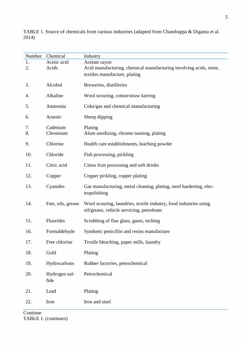
FIGURE 1.Industrial wastewater classification (adapted from Chandrappa & Diganta 2014)

Figure 2 show the classification of dissolved solids on biodegradability. The distillery, dye, electroplat-

ing, electropolishing, pharmaceutical, sugar and surface coating industries discharge effluents which

contain a lot dissolved solid. Some factories such as pharmaceutical manufacture, dye can produce dif-

ferent kind of pollutants which varies from day to day because these sectors want to meet the demand

within the market. (Chandrappa & Diganta 2014) The source of the chemical contamination in the in-

dustrial wastewater varies from factory to factory. Table 1 lists the sources of the chemicals from differ-

ent industries.

FIGURE 2. Classification of dissolved solids based on biodegradability (adapted from Chandrappa &

Diganta 2014)

Wastewater

High BOD

High COD

High inorganic solids

ex: some drugs / durg

intermediates

Low inorgancic solids

ex: spent wash distillery

Low COD


ex: sugar

Low inorganic solids

ex: ready to eat food

Low BOD

High COD


ex: some dye intermediates


ex: some drugs / drug

intermediates

Low COD


ex: metal extraction


ex: bolier / cooling tower

blow down

Inorganic

Organic non-biodegradable

Organic Biodegradable

5

TABLE 1. Source of chemicals from various industries (adapted from Chandrappa & Diganta et al.

2014)

Number Chemical Industry

1. Acetic acid Acetate rayon

2. Acids Acid manufacturing, chemical manufacturing involving acids, mine,

textiles manufacture, plating

3. Alcohol Breweries, distilleries

4. Alkaline Wool scouring, cotton/straw kiering

5. Ammonia Coke/gas and chemical manufacturing

6. Arsenic Sheep dipping

7. Cadmium Plating

8. Chromium Alum anodizing, chrome tanning, plating

9. Chlorine Health care establishments, leaching powder

10. Chloride Fish processing, pickling

11. Citric acid Citrus fruit processing and soft drinks

12. Copper Copper pickling, copper plating

13. Cyanides Gas manufacturing, metal cleaning, plating, steel hardening, elec-

tropolishing

14. Fats, oils, grease Wool scouring, laundries, textile industry, food industries using

oil/grease, vehicle servicing, petroleum

15. Fluorides Scrubbing of flue glass, gases, etching

16. Formaldehyde Synthetic penicillin and resins manufacture

17. Free chlorine Textile bleaching, paper mills, laundry

18. Gold Plating

19. Hydrocarbons Rubber factories, petrochemical

20. Hydrogen sul-

fide

Petrochemical

21. Lead Plating

22. Iron Iron and steel

Continue

TABLE 1. (continues)

6

Number Chemical Industry

23. Mercaptans Oil refining, pulp

24. Nickel Plating

25. Nitro compounds Chemical works and explosives

26. Organic acids Fermentation plants and distilleries

27. Pesticides Pesticide manufacturing

28. Phenols Gas and coke manufacturing, chemical plants

29. Phosphate Soap and detergent

30. Radioactive ma-

terial

Atomic power station, radioactive processing industry

31. Silver Plating

32. Sodium Fish processing, pickling

33. Starch Food processing, textile industries

34. Sugars Breweries, dairies, sweet industry, confectionaries, fruit juice, soft

drink, sugar, jaggary

35. Sulfides Textile industry, tanneries, gas manufacture

36. Tannic acid Tanning, sawmills

37. Tartaric acid Wine, leather, chemical manufacture, dyeing

38. Tin Electroplating

39. Zinc Zinc plating, rubber process, galvanizing

2.1.2 Domestic wastewater

In this section, the definition, characteristics of the domestic wastewater and the methods of measuring

the degree of the domestic wastewater will be described briefly. According to the Finnish decree, do-

mestic wastewater means wastewater originating from water closets of dwellings, offices, business

premises and other facilities, and from kitchens, washing facilities and similar facilities and equipment,

and wastewater with similar properties and composition originating from milk stores at dairy farms or

resulting from other business operations. (Finnish Ministry of the Environment 2003/542.)

7

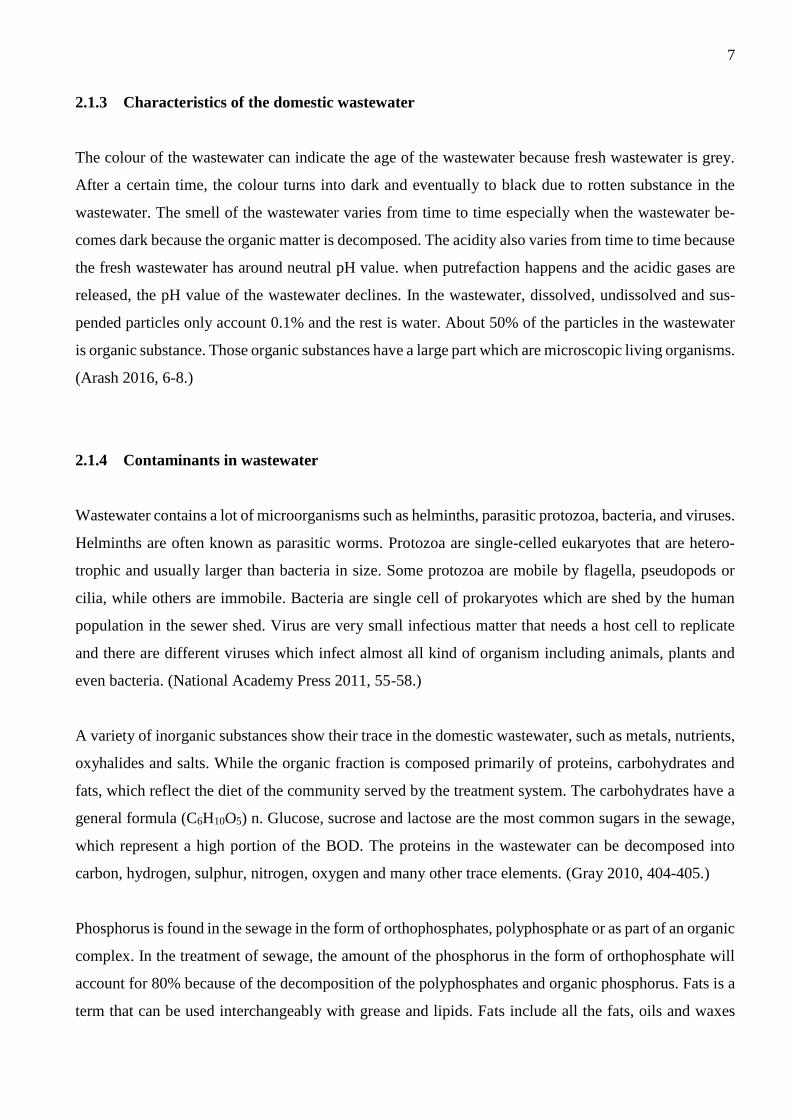
2.1.3 Characteristics of the domestic wastewater

The colour of the wastewater can indicate the age of the wastewater because fresh wastewater is grey.

After a certain time, the colour turns into dark and eventually to black due to rotten substance in the

wastewater. The smell of the wastewater varies from time to time especially when the wastewater be-

comes dark because the organic matter is decomposed. The acidity also varies from time to time because

the fresh wastewater has around neutral pH value. when putrefaction happens and the acidic gases are

released, the pH value of the wastewater declines. In the wastewater, dissolved, undissolved and sus-

pended particles only account 0.1% and the rest is water. About 50% of the particles in the wastewater

is organic substance. Those organic substances have a large part which are microscopic living organisms.

(Arash 2016, 6-8.)

2.1.4 Contaminants in wastewater

Wastewater contains a lot of microorganisms such as helminths, parasitic protozoa, bacteria, and viruses.

Helminths are often known as parasitic worms. Protozoa are single-celled eukaryotes that are hetero-

trophic and usually larger than bacteria in size. Some protozoa are mobile by flagella, pseudopods or

cilia, while others are immobile. Bacteria are single cell of prokaryotes which are shed by the human

population in the sewer shed. Virus are very small infectious matter that needs a host cell to replicate

and there are different viruses which infect almost all kind of organism including animals, plants and

even bacteria. (National Academy Press 2011, 55-58.)

A variety of inorganic substances show their trace in the domestic wastewater, such as metals, nutrients,

oxyhalides and salts. While the organic fraction is composed primarily of proteins, carbohydrates and

fats, which reflect the diet of the community served by the treatment system. The carbohydrates have a

general formula (C6H10O5) n. Glucose, sucrose and lactose are the most common sugars in the sewage,

which represent a high portion of the BOD. The proteins in the wastewater can be decomposed into

carbon, hydrogen, sulphur, nitrogen, oxygen and many other trace elements. (Gray 2010, 404-405.)

Phosphorus is found in the sewage in the form of orthophosphates, polyphosphate or as part of an organic

complex. In the treatment of sewage, the amount of the phosphorus in the form of orthophosphate will

account for 80% because of the decomposition of the polyphosphates and organic phosphorus. Fats is a

term that can be used interchangeably with grease and lipids. Fats include all the fats, oils and waxes

8

associated with food. Because of the stability of the fats, the forms of the fats presenting in the sewage

usually are palmitic, oleic and stearic. These fats can contribute a significant BOD of wastewater (40-

100 mg/l). Nitrogen (N) exists in different forms in the sewage such as organic nitrogen, ammonia and

oxidized nitrogen (nitrate and nitrite). (Gray 2010, 404-405.)

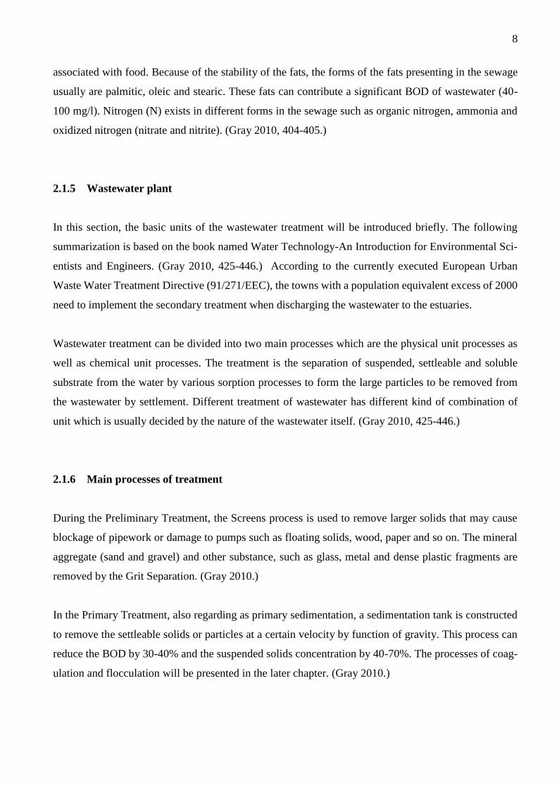
2.1.5 Wastewater plant

In this section, the basic units of the wastewater treatment will be introduced briefly. The following

summarization is based on the book named Water Technology-An Introduction for Environmental Sci-

entists and Engineers. (Gray 2010, 425-446.) According to the currently executed European Urban

Waste Water Treatment Directive (91/271/EEC), the towns with a population equivalent excess of 2000

need to implement the secondary treatment when discharging the wastewater to the estuaries.

Wastewater treatment can be divided into two main processes which are the physical unit processes as

well as chemical unit processes. The treatment is the separation of suspended, settleable and soluble

substrate from the water by various sorption processes to form the large particles to be removed from

the wastewater by settlement. Different treatment of wastewater has different kind of combination of

unit which is usually decided by the nature of the wastewater itself. (Gray 2010, 425-446.)

2.1.6 Main processes of treatment

During the Preliminary Treatment, the Screens process is used to remove larger solids that may cause

blockage of pipework or damage to pumps such as floating solids, wood, paper and so on. The mineral

aggregate (sand and gravel) and other substance, such as glass, metal and dense plastic fragments are

removed by the Grit Separation. (Gray 2010.)

In the Primary Treatment, also regarding as primary sedimentation, a sedimentation tank is constructed

to remove the settleable solids or particles at a certain velocity by function of gravity. This process can

reduce the BOD by 30-40% and the suspended solids concentration by 40-70%. The processes of coag-

ulation and flocculation will be presented in the later chapter. (Gray 2010.)

9

Biological treatment is a significant sector of domestic wastewater plant, where the wastewater is mixed

or exposed to a dense microbial organism under aerobic environment. And the Secondary treatment will

separate the dense microbial biomass from the purified wastewater. (Gray 2010.)

The tertiary treatment is set when the secondary treatment can’t meet the requirements. Filtration, disin-

fection processes are usually implemented. Chlorination of effluents is common accepted in the USA,

while ozonation or ultraviolet is widely used in Europe because it has less impact on the environment.

(Gray 2010.)

FIGURE 3.Basic flowchart of wastewater treatment plant (adapted from Gray 2010)

Influent

Preliminary

treatment

Primary

treatment

Secondary

treatment

Secondary

sedimentation

Coarse screens

Fine screens

Grit separation

Flotation

Primary sedimentation

Mixed aeration

Tertiary

treatment

Sludge

treatment

Membrane filtration

Disinfection

Coagulation, Flocculation

10

2.2 Turbidity of wastewater

Turbidity is the measure of the clarity of a liquid. It is contributed by both suspended solids and colloidal

material in water. Most of the turbidity in surface water is due to the erosion of colloidal substances like

clay, silt, rock fragments, microbes and so on. The units of measurements are the Jackson Turbidity Unit

(JTU), the Formazine Turbidity Unit (FTU) and the Nephelometry Turbidity Unit (NTU). The proce-

dures/instruments for measuring each of these units vary considerably. (Chandrappa 2014.)

The turbidity is mostly created by the suspended solid in water. Suspended solid means any substance

suspended in water qualifies as a suspended solid. It is determined by filtration followed by weighing of

filter paper after drying and subtracting the weight of the filter paper. It is represented as mg/l. The

suspended solids are characteristics of surface water bodies and wastewater from domestic as well as

industrial/trade effluents. (Chandrappa 2014.)

2.3 Coagulation and flocculation

Hopeakivenlahti WWTP has the processes of coagulation and flocculation. The coagulant PIX-105 is

introduced into the following processes such as pretreatment, after primary sedimentation, flotation. And

the coagulant aid is only added into the flotation process. (adapted from Sydänmetsä 2018.) The figure

4 shows the basic flowchart of dosing the chemical reagents.

FIGURE 4.Flowchart of coagulant dosing and coagulant aid in Hopeakivenlahti WWTP (adapted from

Sydänmetsä 2018)

11

Coagulation is one of the chemical processes to remove turbidity and color producing material that is

mostly colloidal particles (1 to 200 millimicrons, m) such as bacteria, organic and inorganic matters,

algae and clay particles. (Lee & Lin 2007, 1.375.) Flocculation is the aggregation of destabilized parti-

cles and sedimentation substances formed by the addition of coagulants into a larger particle known as

‘floc’. The most common method which is implemented to reduce the particulate substance and a portion

of the dissolved NOM from the surface water is by sedimentation and/or filtration following the condi-

tioning of the water by coagulation and flocculation. (R Rhodes &John 2012, 140.) Figure 5 shows the

conventional treatment process of flow diagram which implements the coagulation.

FIGURE 5.Typical wastewater process employing coagulation with conventional treatment, direct fil-

tration or contact filtration (adapted from Trussell & John 2012)

2.4 Stability of particles in water

The Brownian motion is when mobile particles are immersed in an ambient medium, the particles un-

dergo an incessant and irregular motion. Stability is one of the characteristics of Brownian motion. The

motion can persist if the particles remain suspended in the liquid. (Robert 2008, 46) Particles in the

wastewater can be categorized as hydrophobic (water repelling) and hydrophilic (water attracting). The

fine particles in water have surface charge, which result to relative stability, causing a long period of

detention of the particles suspended in water. There are four common kind of origination of the particle

surface charge: Isomorphous Replacement (Crystal Imperfections), Structural Imperfections, Preferen-

tial Adsorption of Specific Ions and Ionization of Inorganic Surface Functional Groups. (Robert 2008,

46)

12

In the water, particles always have a negative surface. Figure 6 shows that a fixed adsorption layer will

form when a layer of cations binds tightly to the surface of a negatively charged particle. This adsorbed

layer of cations, stick to the surface of particle by adsorption forces and electrostatic, is about 0,5nm

thick and is known as the Helmholtz layer (interchangeably with Stern layer). (Trussell & John 2012,

145.)

FIGURE 6. Structure of the electrical double layer (adapted from Trussell &John 2012, 145)

The layer of anions and cations which extends form the Helmholtz layer to the bulk solution where the

charge is zero and electroneutrality is satisfied is known as the diffuser layer. Both adsorbed and diffuse

layer are regarded as the electric double later (EDL), which can reach up to 30 nm wide in the solution

depending on the solution characteristics. (Trussell &John 2012, 145.)

The stability of particles in natural waters depends on a balance between the repulsive electrostatic force

of the particle and the attractive forces known as the van der Waals forces. Van der Waals attractive

forces are strong enough to overcome electrostatic repulsion but they are not able to do so because the

EDL and electrostatic extend further than do the van der Waals forces in the solution. To destabilize

particles, the energy of the electrostatic repulsion needs to be overcome. (Trussell &John 2012, 145.)

13

2.5 Principles of coagulation and flocculation

There are four main mechanisms regarding the principles of coagulation: compression of the electric

double layer, adsorption and charge neutralization, adsorption and inter-particle bridging and enmesh-

ment in a precipitate which is also known as ‘‘sweep floc’’. Through adsorption of oppositely charged

ions or polymer, particles can be destabilized. Positively charged hydrolyzed metal salts, prehydrolyzed

metal salts and cationic organic polymers can be utilized to destabilize particles by neutralizing the

charge on the particle surface. If the charge is neutralized in surface of particle, then the EDL will dis-

appear and van der Waals force can easily make particles to stick together. Polymer chains adsorb on

particle surfaces at one or more sites along the chain with a result of coulombic (charge-charge) interac-

tions, dipole interaction, hydrogen bonding and van der Waals forces of attraction. After dosing enough

aluminum or iron, they will form insoluble sedimentation and particles become entrapped in the amor-

phous precipitates. (Trussell &John 2012, 149.)

Flocculation includes the following mechanisms: small particles experience random Brownian motion

due to collisions with fluid molecules resulting in particle-particle collisions; particles collisions happens

because of the velocity gradients created by stirring water containing particles; These two interactions

are also known as microscale and macroscale flocculation. (Trussell &John 2012, 165.)

Generally, the internal between coagulation and flocculation in very instant, almost at the same time

during the wastewater treatment. The coagulation-flocculation can be classified into three stages: (a)

drug dispersion and its interaction with particles (defined as mixing effect); (b) coagulation effect; (c)

flocculation. (Hanhui, Xiaoqi & Xuehui 2004.) Figure 7 shows the physical models of coagulation-floc-

culation process.

14

FIGURE 7. Physical models of coagulation-flocculation process (adapted from Hanhui, Xiaoqi &

Xuehui 2004)

2.6 Coagulant and flocculant

Basically, the coagulant used widely in wastewater treatment plant are chloride or sulfide salts or alu-

minum and ferric ions and prehydrolyzed salts of these metals while flocculant can be classified into

natural and synthetic kinds. (Trussell & John 2012.) In this part, the kinds of coagulant and flocculant

are introduced briefly and their functional mechanism are mentioned.

15

2.6.1 Coagulant

The common used inorganic coagulants in the wastewater plant are chloride or sulfide salts of aluminum,

ferric ions and prehydrolyzed salts of these metals. These metal cations are readily available in both dry

and liquid form. Aluminum sulfate or “alum” is favored by a lot of WWTP, which is solid in hydrated

form as Al2(SO4)3•H2O, where is normally about 14. When aluminum or ferric ions are introduced

into wastewater, a certain number of sequential reactions happen. Firstly, the salt of Al(III) and Fe(III)

will dissociate to produce trivalent Al3+ and Fe3+ ions, as shown below: (Trussell & John 2012.)

Al2(SO4)3 ⇄ 2Al3+ + 3SO42- (1)

FeCl3 ⇄ Fe3+ + 3Cl- (2)

The ions of Fe3+ and Al3+ then hydrate to form the aquometal complexes Al(H2O)63+ and Fe(H2O)6

3+,

as presented in the left side of the equation (3)

(3)

Then a variety of soluble mononuclear Al(H2O)5(OH)2+, Al(H2O)4(OH)2+, Al(H2O)3(OH)3

0 and poly

nuclear Al18(OH)204+, (Al8(OH)20•28H2O)4+ form in the water. Similarly, iron forms a variety of soluble

species, such as mononuclear Fe(H2O)5(OH)2+ and Fe(H2O)4(OH)2+. These polynuclear and mononu-

clear species can interact with the particles in the water, depending on the characteristics of substances

in the wastewater. (Trussell &John 2012)

The solubility of the different iron Fe(III) and alum Al(III) are illustrated in Figure 8. Figure 8 shows

that the ferric species are more insoluble than aluminum species and are also insoluble in a wider pH

range. Ferric ion is the good choice for the destabilization. (Trussell &John 2012)

H2O OH2 3+

H2O Me OH2

H2O OH2

H2O OH 2+

H2O Me OH2

H2O OH2

+ H+

16

FIGURE 8. Solubility diagram for (a) Al(III) and (b) Fe(III) at 25C (adapted from Trussell &John et

al. 2012,152.)

When the alum or ferric sulfate is added into the wastewater, the overall precipitation reactions are as

follows:

Al2(SO4)3•14H2O → 2Al(OH)3(s) + 6H+ + 3SO42- + 8H2O (4)

Fe2(SO4)3•9H2O → 2Fe(OH)3(s) +6H+ +3SO42- + 3H2O (5)

2.6.2 Flocculant

The basic aim of water and wastewater treatment is to make slowly aggregating suspension become a

quick aggregating suspension. (Olufemo 2004,11.) Flocculant, interchangeably with coagulant aid, is a

substance that is used in conjunction with a primary coagulant, to enhance coagulation. Flocculant can

be classified into natural and synthetic kinds. Further, coagulant aid can be categorized as cationic, ani-

onic, or nonionic polymers and of low, medium, or high molecular weight. (Olufemo 2004.)

Nowadays, the synthetic organic polymers play a significant role in the wastewater treatment. (AWWA

Staff 2010, 36.) Because the synthetic organic polymers are much cheaper than those made from natural

sources. Synthetic organic polymers are made either by homopolymerization of the monomer or by co-

polymerization of two monomers. Further, the polymer synthesis can be controlled to produce polymers

of different size (molecular weight), charge groups, number of charge groups per polymer chain (charge

density), and varying structure (linear or branched). Table show the principal synthetic organic polymers

used for water treatment. (John 2012, 575.)

17

TABLE 2. Typical organic coagulant aids used in the water treatment (adapted from John 2012, 575.)

Type Charge

Molecular

Weight,

g/mole

Common

Applications Typical Examples Other Examples

Anionic Negative 104-107

Coagulant

aid, filter aid,

flocculant

aid, sludge

conditioning

Hydrolyzed

polyacrylamides

Hydrolyzed

polyacrylamides,

polyacrylates,

polyacrylic acid, poly

styrene, sulfonate

Cationic Positive 104-106

Primary

coagulant,

turbidity and

color

removal

Epichlorohydrin

dimethylamine

Aminomethyl

polyacrylamide,

polyalkylene,

polyamines,

polyethylenimine

Sludge

condition

Polydiallyldimethyl

ammonium

chloride (poly-

DADMAC)

Polydimethyl

aminomethyl

polyacrylamide,

polyvinylbenzyl,

trimethyl ammonium

chloride

Nonionic Neutral 105-107

Coagulant

aid, filter aid,

filter

conditioning

Polyacrylamides Polyacrylamides,

polyethylene oxide

Others Variable Variable - Sodium alginate

Alginic acid, dextran,

guar gum, starch

derivatives

2.7 Jar test

For over 50 years, the jar test has been the standard tool implemented to optimize the addition of coag-

ulants and flocculants used in the wastewater and drinking water treatment industry. (Ebeling, Sibrell,

18

ogden & Summerflt 2003, 28) The jar test is evaluated as a valuable tool by water industry for realisti-

cally simulating coagulation, flocculation, and sedimentation at a full-scale treatment plant. The jar test

may be done for many different reasons. By conducting the test, result can be utilized to evaluate the

influences of the changes in chemical dosages and points of application; choose alternative coagulants;

vary mixing intensity and times; add polymeric coagulant aids; implement alternative preoxidation strat-

egies; and change the overflow rates on the removal of particles, NOM, or other water quality parameters

of concern. It is significant that the condition of the jar test accurately simulates the full-scale plant

conditions. There are several key parameters shown as following:

Effective retention times in the rapid mix and flocculation basins

Velocity gradient/mixing intensity in the rapid mix and flocculation basins

Surface loading rate of the sedimentation basin

Real retention time in basins if jar testing is being done to evaluate time-dependent reactions for

which full-scale reaction time influences results. (Ebeling, Sibrell, ogden & Summerflt 2003.)

If a successful jar test is performed, there is usually a need to empirically tweak the parameters to make

the jar test result corresponding to the full-scale results. There is a common result of the limitations of

the jar test in matching the physical characteristics of the treatment process. Even the jar tests are per-

formed to assist full-scale plant optimization, they may also be conducted to meet certain regulatory

requirements. Under the Stage 1 Disinfectants and Disinfection By-products Rule (D/DBPR) (1998), jar

testing may be conducted as part of the “enhanced coagulation” requirements. (AWWA Staff 2010, 17-

18.)

2.7.1 Parameters concerned in Jar Test

The velocity gradient, G, refers to the intensity of mixing, with units of s-1 (seconds to the power of

minus 1). The velocity gradient is calculated by using the energy dissipation rate in the fluid, or it can

be interpolated from calibration curves. It should be noted that the velocity gradient varies significantly

with water temperature (because of viscosity is associated with temperature) independent of the mixing

device speed. So, it is better to simulate the temperature in the jar testing’s condition which is the same

as plant water’s temperature. (AWWA Staff 2010, 18)

19

Initial mixing or rapid mix is the process which happens when the coagulant is added into the wastewater.

It is better to conduct the rapid mix’s condition which match the full-scale conditions as much as possi-

ble. The typical mixing intensities for a well-designed flash mix tank range from 700 to 1,000 s-1, and

for a typical jar test, 30-60 seconds of retention time is used, with high paddle speeds of 100-300 rpm.

It should be noted that during the determination of the optimal initial mixing intensity, the other basic

parameters should be conducted first such as, the preferable chemical coagulant dose, pH and alkalinity.

(AWWA Staff 2010, 18-19.)

Flocculation’s retention time and G values should correspond to those in the WWTP when conducting

the jar testing. After dosing the coagulant and flash mixing, the coagulant aid is introduced into the

flocculation basin where the typical retention times ranges from 15 to 30 minutes are conducted, while

the mixing intensities vary from 10 to 40 s-1. It should be noticed that the flocculation intensity should

not be too low or too high, because too light intensity can’t contribute to form big flocs while too high

intensity will break the floc into small particles again. (AWWA Staff 2010, 19.)

Sedimentation time is considered carefully to optimize the floc development and settleability. The set-

tling velocity of floc must be higher than the surface loading rate of the clarification basin, otherwise the

floc won’t settle. (AWWA Staff 2010, 19-20). The points of chemical applications are one of the popular

topics in the jar testing. If the purpose of the jar test is to optimize the conditions for an existing full -

scale plant, chemical reagents need to be added in the same order as in the plant. Alternatively, the same

reagents can be added in a different order or at different times aiming to enhance the quality of water

produced. (AWWA Staff 2010, 20)

2.7.2 Configuration of Jar Test

Jar test equipment consists of jars to contain the water, the impeller, the mechanism to drive the impeller

and lab equipment to analyze the results. Figure 9 shows the typical jars used in the jar testing. Usually

the jars are 2-L square beakers. (AWWA Staff et al, 2010, 25.)

20

FIGURE 9. Jar test unit (adapted from AWWA Staff et al, 2010, 25.)

21

3 EXPERIMENT

Experiments are mainly based on the theory of Jar test. But because of the limitation of the equipment,

a similar equipment was built to replace the standard jar test equipment. The main parameters are tur-

bidity and the coagulant residual (iron concentration). The experiment can be divided into six parts as

following.

1. Characteristics of the raw wastewater

2. Optimal operation condition of coagulant

3. Effect of initial mixing intensity (flash mixing)

4. Effect of flocculation mixing intensity

5. Effect of flocculation mixing time

The data collected from these five experiments will be presented and analyzed in the results and dis-

cussion chapter.

3.1 Basic chemical reagents and source of wastewater

The coagulant used in the experiment was obtained from the Hopeakivenlahti WWTP. The coagulant is

ferric sulfate solution (PIX-105) which is manufactured by Kemira. The technical data sheet of the PIX-

105 can be found in the appendix. The coagulant aids used in the experiment was obtained from the

Hopeakivenlahti WWTP as well. The coagulant aid is kind of polymer whose model is LC2218 manu-

factured by Finland Cleartech company. The analytical base and acid used in the experiment were so-

dium hydroxide and hydrogen chloride. All the experimental wastewater was obtained from the Hopeak-

ivenlahti WWTP. For different experiment, the sampling sites were different. Details of sampling will

be described latter.

3.2 Main equipment

The rotational stirring machine and the paddle were used in the experiment. The paddle was washed by

the distilled water before it was used in the experiment. The turbidity meter was calibrated every time

before it was used. Figure 10 shows the model of the stirrer and turbidity meter.

22

FIGURE 10. Rotational stirrer(left), paddle (middle) and Turbidity meter (right)

All of samples which were needed to be analyzed by atomic absorption spectroscopy (AAS) in the ex-

periment were filtrated by the 0.45 m filter disk. The AAS analyzer used in the determination of iron

concentration is PerkinElmer AAnalyst 200.

FIGURE 11. Syringe and filter disk (left) and AAS analyzer (right)

23

3.3 Basic calculation

The density of the coagulant and coagulant aid is 1.55 ± 0.05 g/cm3 and 1100-1200 kg/m3. Because the

dosing of the chemical was according to the volume. The volume of coagulant and coagulant aid was

calculated by equation (1).

𝑣 =𝑚

𝜌 (1)

During the experiment, the pH of the raw wastewater sometimes needed to be adjusted to preferable

value, which was achieved by adding either sodium hydroxide or hydrogen chlorine into the raw

wastewater. The following calculation steps were performed during the experiment. For adding the hy-

drogen chlorine, the volume of the acid was obtained by the following equation (2). For adding the

sodium hydroxide, the volume of the base was obtained by the following equation (3).

𝑣 =𝑥×(10−𝑦−10−𝑧)

10−𝑧−𝑀 (2)

v: volume of hydrogen chlorine, L

x: volume of raw wastewater, L

y: pH of the raw wastewater

z: desire pH of wastewater

M: molarity of hydrogen chlorine, mole/L

𝑣 =𝑥×(10−𝑦−10−𝑧)

10−𝑧+𝑀 (3)

v: volume of sodium hydroxide, L

x: volume of raw wastewater, L

y: pH of the raw wastewater

z: desire pH of wastewater

M: molarity of sodium hydroxide, mole/L

24

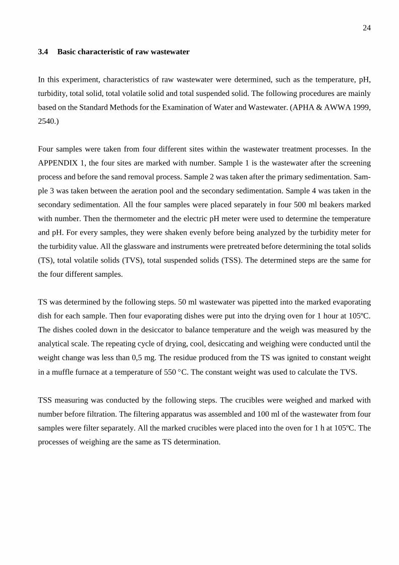
3.4 Basic characteristic of raw wastewater

In this experiment, characteristics of raw wastewater were determined, such as the temperature, pH,

turbidity, total solid, total volatile solid and total suspended solid. The following procedures are mainly

based on the Standard Methods for the Examination of Water and Wastewater. (APHA & AWWA 1999,

2540.)

Four samples were taken from four different sites within the wastewater treatment processes. In the

APPENDIX 1, the four sites are marked with number. Sample 1 is the wastewater after the screening

process and before the sand removal process. Sample 2 was taken after the primary sedimentation. Sam-

ple 3 was taken between the aeration pool and the secondary sedimentation. Sample 4 was taken in the

secondary sedimentation. All the four samples were placed separately in four 500 ml beakers marked

with number. Then the thermometer and the electric pH meter were used to determine the temperature

and pH. For every samples, they were shaken evenly before being analyzed by the turbidity meter for

the turbidity value. All the glassware and instruments were pretreated before determining the total solids

(TS), total volatile solids (TVS), total suspended solids (TSS). The determined steps are the same for

the four different samples.

TS was determined by the following steps. 50 ml wastewater was pipetted into the marked evaporating

dish for each sample. Then four evaporating dishes were put into the drying oven for 1 hour at 105ºC.

The dishes cooled down in the desiccator to balance temperature and the weigh was measured by the

analytical scale. The repeating cycle of drying, cool, desiccating and weighing were conducted until the

weight change was less than 0,5 mg. The residue produced from the TS was ignited to constant weight

in a muffle furnace at a temperature of 550 C. The constant weight was used to calculate the TVS.

TSS measuring was conducted by the following steps. The crucibles were weighed and marked with

number before filtration. The filtering apparatus was assembled and 100 ml of the wastewater from four

samples were filter separately. All the marked crucibles were placed into the oven for 1 h at 105ºC. The

processes of weighing are the same as TS determination.

25

3.5 Optimal dose and dosing conditions of coagulant

In this set of experiment, the optimal dose of the coagulant and pH were determined by the mean of jar

test. There are three steps for this determination. The turbidity and the coagulant residual (iron concen-

tration) were measured as for the parameters. Except the dose of the coagulant and the pH, the temper-

ature, dose of coagulant aid was kept the same as the Hopeakivenlahti WWTP because this is regarded

as the optimal dose in the Hopeakivenlahti wastewater treatment plant. The dose of coagulant aid used

in the Hopeakivenlahti WWTP is 10 g/m3 (Sydänmetsä 2018).

3.5.1 Optimal dose of coagulant

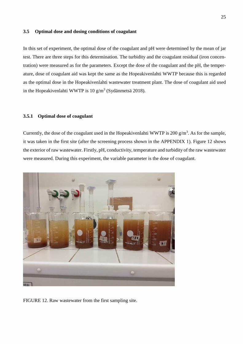
Currently, the dose of the coagulant used in the Hopeakivenlahti WWTP is 200 g/m3. As for the sample,

it was taken in the first site (after the screening process shown in the APPENDIX 1). Figure 12 shows

the exterior of raw wastewater. Firstly, pH, conductivity, temperature and turbidity of the raw wastewater

were measured. During this experiment, the variable parameter is the dose of coagulant.

FIGURE 12. Raw wastewater from the first sampling site.

26

Table 2 shows that the beakers were numbered from 0 to 6. The volume of the wastewater used in the

experiment was 500 ml. As shown in the last paragraph, the dose of coagulant aid used in the Hopeak-

ivenlahti WWTP was 200 g/m3 which is converted to 4,35 microliters by equation (1). The different

volume of coagulant used during the experiment are shown in the table as well.

TABLE 2. Determination of optimal coagulant dose

Number 0 1 2 3 4 5 6

Sample volume (ml) 500

Coagulant aid (l) 4,35

Coagulant dose (g/m3) 0 100 150 200 250 300 350

Coagulant dose (l) 0 6,45 9,67 12,90 16,12 19,35 22,57

Because there is only one rotational stirrer, all the samples were treated one by one. Firstly, the sample

was put under the stirrer and the stirrer was operated at 100 rpm. The coagulant was added first according

to the Table 2, starting the timer at the same time. After 1 minute, the coagulant aid was dosed and the

stirrer was operated in 20 rpm for 15 minutes. Then beaker was moved out from the stirrer, waiting for

another 15 minutes for settling. Figure 13 shows the coagulation and flocculation process.

FIGURE 13. Coagulation (left) and flocculation (right)

The 40 ml pipette was used to move 40 ml supernatant of the sample into a glass vial for the turbidity

determination. The filtration apparatus was set up to filtrate the sample by 0,45 m membrane and filtrate

27

was collected for the ion concentration determination. The ion concentration was analyzed by the AAS.

From the APPENDIX 2, the calibration of the iron concentration and the method used in the determina-

tion are shown. After collecting the data, two simple curves were drawn which shows the turbidity

against coagulant dose and the ion concentration against the coagulant dose. These curves will be shown

in the results and discussion chapter.

3.5.2 Optimal dosing pH

The second step aimed to determine the optimal dosing pH. The pH of the raw wastewater was altered

by adding either acid or alkali. Then the jar tests were repeated using the optimal coagulant dose deter-

mined in the first set of the tests. Table 4 shows the pH, volume of sample, coagulant and coagulant aid

used in this set of jar test. The optimal coagulant aid is 100 g/cm3 which was obtained by analyzing the

curve made in the first step. Details about the optimal coagulant aid can be found in the RESULTS AND

DISSCUSSION chapter.

TABLE 4. Determination of optimal pH

Number of the sample 0 1 2 3 4 5 6

pH 2.99 3.5 4.5 5 5.5 6 6.5

Coagulant dose (g/m3) 0 100

Coagulant dose (l) 0 6.45

Coagulant aid (l) 0 4,35


After conditioning the pH of the raw samples, the coagulant was added first and under initial mixing of

100 rpm for 1 minute. While coagulant aid was added, the mixing intensity was switched to 20 rpm for

15 minutes. Then beaker was moved out from the stirrer, waiting another 15 minutes for settling.

The 40 ml pipette was used to move 40 ml supernatant of the sample into a glass vial for the turbidity

determination. The filtration apparatus was set up to filtrate the sample by 0,45 m membrane and filtrate

was collected for the ion concentration determination. The ion concentration was analyzed by the AAS.

28

From the APPENDIX 2, the calibration of the iron concentration and the method used in the determina-

tion are shown. After collecting the data, two simple curves were drawn which show the turbidity against

pH and the iron concentration against the pH. These curves will be shown in the results and discussion

chapter.

3.5.3 Re-determination of the optimal coagulant dose

The test was repeated by using raw wastewater but this time wastewater was corrected to the optimal pH

and tested at various coagulant doses again (Gray 2010). The optimal pH is 4.5 which was obtained by

analyzing the curve made in the second step. Details about the optimal pH can be found in the results

and discussion chapter. Table 5 shows the parameters concerned in the experiment.

TABLE 5. Re-determination of the optimal coagulant dose

Number 0 1 2 3 4 5 6

Coagulant dose (g/m3) 0 50 100 150 200 250 300

Coagulant dose(l) 0 3.225 6,45 9,675 12,9 16,125 19.35


pH 4.5


The initial mixing intensity was 100 rpm for 1 minute and the flocculation mixing intensity was 20 rpm

for 15 minutes. Then another 15 minutes were for the floc settling. The supernatant was taken for the

turbidity determination. The filtrate of the treated samples was analyzed by AAS for the iron concentra-

tion determination. When the data was collected, two curves were drawn which shows the turbidity

against the coagulant dose and the iron concentration against coagulant dose. From the curves, the opti-

mal dose of coagulant can be found at the pH of 4,5. These curves will be shown in the results and

discussion chapter.

29

3.6 Effect of initial mixing intensity

From the “Optimal dose and dosing conditions of coagulant” section, the optimal dose of coagulant and

the dosing pH were found and used to determine the effect of initial mixing intensity. In part of experi-

ment, the pH of the raw sample was adjusted to the optimal value first. The equipment was prepared for

another set of jar testing. During the experiment, the variable value was the intensity of initial mixing

intensity. Table 6 shows the parameters concerned in this experiment.

TABLE 6. Effect of initial mixing intensity

Number 0 1 2 3 4

Mixing intensity(rpm) 0 50 100 140 170

pH 4,5

Wastewater volume (ml) 500

Coagulant dose(l) 6,45


For the first sample, after dosing the coagulant, the initial mixing intensity was set at 50 rpm for 1 minute.

Then the flocculation mixing intensity was at 20 rpm for 15 minutes after dosing the coagulant aid.

Another 15 minutes was for the settling of floc. Supernatant was collected for the turbidity determina-

tion. The treated sample was filtrated by 0,45 m membrane for the determination of iron concentration

by AAS. Except varying the initial mixing intensity, the other operational processes were kept as the

same as the treatment of first sample. Finally, the two curves which show the turbidity against the initial

mixing intensity and iron concentration against initial mixing intensity were illustrated. These curves

will be shown in the results and discussion chapter.

3.7 Effect of flocculation mixing intensity

The optimal dose of coagulant and the dosing pH obtained from the “Optimal dose and dosing conditions

of coagulant” part was used to determine the effect of flocculation mixing intensity as well. The pH of

30

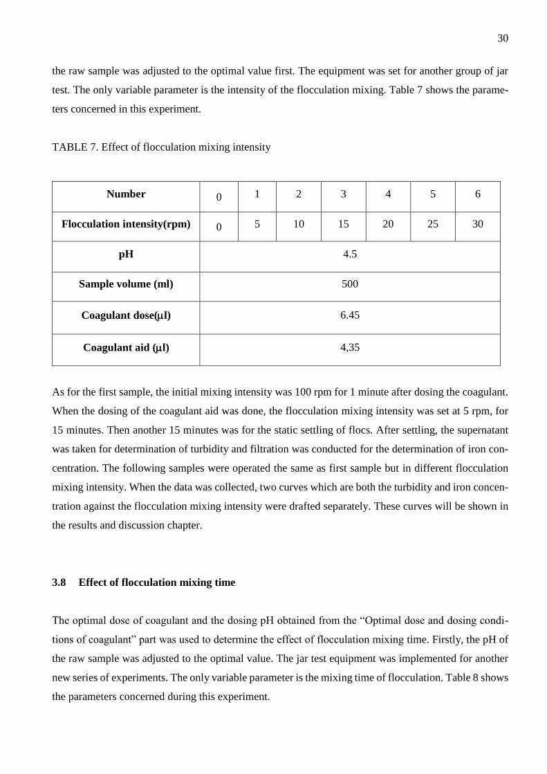
the raw sample was adjusted to the optimal value first. The equipment was set for another group of jar

test. The only variable parameter is the intensity of the flocculation mixing. Table 7 shows the parame-

ters concerned in this experiment.

TABLE 7. Effect of flocculation mixing intensity

Number 0 1 2 3 4 5 6

Flocculation intensity(rpm) 0 5 10 15 20 25 30

pH 4.5


Coagulant dose(l) 6.45


As for the first sample, the initial mixing intensity was 100 rpm for 1 minute after dosing the coagulant.

When the dosing of the coagulant aid was done, the flocculation mixing intensity was set at 5 rpm, for

15 minutes. Then another 15 minutes was for the static settling of flocs. After settling, the supernatant

was taken for determination of turbidity and filtration was conducted for the determination of iron con-

centration. The following samples were operated the same as first sample but in different flocculation

mixing intensity. When the data was collected, two curves which are both the turbidity and iron concen-

tration against the flocculation mixing intensity were drafted separately. These curves will be shown in

the results and discussion chapter.

3.8 Effect of flocculation mixing time

The optimal dose of coagulant and the dosing pH obtained from the “Optimal dose and dosing condi-

tions of coagulant” part was used to determine the effect of flocculation mixing time. Firstly, the pH of

the raw sample was adjusted to the optimal value. The jar test equipment was implemented for another

new series of experiments. The only variable parameter is the mixing time of flocculation. Table 8 shows

the parameters concerned during this experiment.

31

TABLE 8. Effect of flocculation mixing time

Number 0 1 2 3 4 5

Flocculation time(minute) 0 5 10 15 20 30

pH 4.5

Sample volume(ml) 500

Coagulant dose(l) 6.45


As for the first sample, when dosing of the coagulant was finished, the initial mixing intensity was set

at 100 rpm for 1 minute. Then after the coagulant aid was added, the flocculation mixing intensity was

operated at 20 rpm for 5 minutes. Another 15 minutes was for the settling of flocs. Finally, the superna-

tant was taken for the turbidity analysis and the treated sample was filtrated to determine the iron con-

centration by AAS. The other samples were treated in the same way but in different flocculation time.

When the data was collected, two curves which are both turbidity and iron concentration against the

flocculation time were drawn. These curves will be shown in the results and discussion chapter.

32

4 RESULTS AND DISCUSSION

In this chapter, the experimental data from the whole work are shown. The data are shown in both table

and graph form. From the graphs, the optimal dose and dosing condition of coagulant, effect of mixing

intensity and mixing time are found during different step within the experiment. There is also explicit

discussion in every step within the experiment.

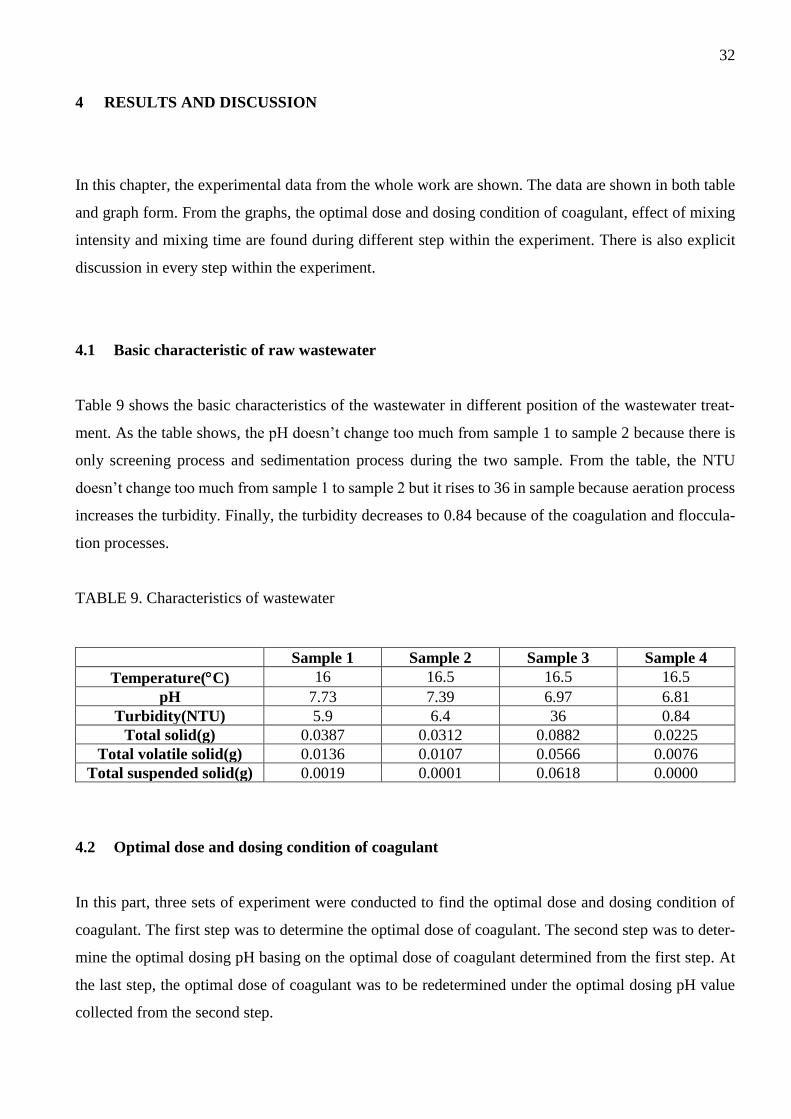
4.1 Basic characteristic of raw wastewater

Table 9 shows the basic characteristics of the wastewater in different position of the wastewater treat-

ment. As the table shows, the pH doesn’t change too much from sample 1 to sample 2 because there is

only screening process and sedimentation process during the two sample. From the table, the NTU

doesn’t change too much from sample 1 to sample 2 but it rises to 36 in sample because aeration process

increases the turbidity. Finally, the turbidity decreases to 0.84 because of the coagulation and floccula-

tion processes.

TABLE 9. Characteristics of wastewater

Sample 1 Sample 2 Sample 3 Sample 4

Temperature(C) 16 16.5 16.5 16.5

pH 7.73 7.39 6.97 6.81

Turbidity(NTU) 5.9 6.4 36 0.84

Total solid(g) 0.0387 0.0312 0.0882 0.0225

Total volatile solid(g) 0.0136 0.0107 0.0566 0.0076

Total suspended solid(g) 0.0019 0.0001 0.0618 0.0000

4.2 Optimal dose and dosing condition of coagulant

In this part, three sets of experiment were conducted to find the optimal dose and dosing condition of

coagulant. The first step was to determine the optimal dose of coagulant. The second step was to deter-

mine the optimal dosing pH basing on the optimal dose of coagulant determined from the first step. At

the last step, the optimal dose of coagulant was to be redetermined under the optimal dosing pH value

collected from the second step.

33

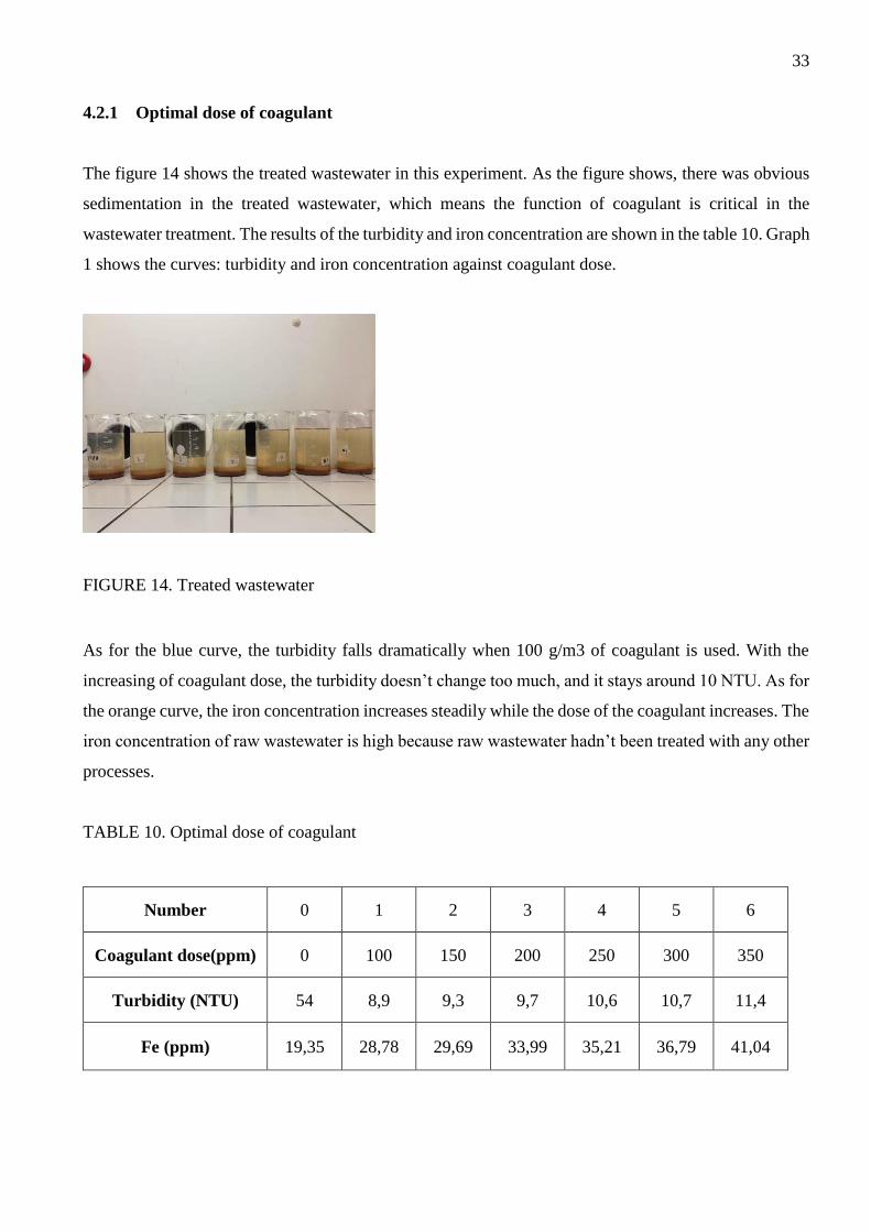
4.2.1 Optimal dose of coagulant

The figure 14 shows the treated wastewater in this experiment. As the figure shows, there was obvious

sedimentation in the treated wastewater, which means the function of coagulant is critical in the

wastewater treatment. The results of the turbidity and iron concentration are shown in the table 10. Graph

1 shows the curves: turbidity and iron concentration against coagulant dose.

FIGURE 14. Treated wastewater

As for the blue curve, the turbidity falls dramatically when 100 g/m3 of coagulant is used. With the

increasing of coagulant dose, the turbidity doesn’t change too much, and it stays around 10 NTU. As for

the orange curve, the iron concentration increases steadily while the dose of the coagulant increases. The

iron concentration of raw wastewater is high because raw wastewater hadn’t been treated with any other

processes.

TABLE 10. Optimal dose of coagulant

Number 0 1 2 3 4 5 6

Coagulant dose(ppm) 0 100 150 200 250 300 350

Turbidity (NTU) 54 8,9 9,3 9,7 10,6 10,7 11,4

Fe (ppm) 19,35 28,78 29,69 33,99 35,21 36,79 41,04

34

In this case, the optimal coagulant dose seems to be the point where the two curves intersect, where the

coagulant dose is around 50 g/m3. But it needs to be noticed that the nature of the raw wastewater varies

too much from time to time, indicating that a buffer needs to be placed to the dose of coagulant. The

optimal coagulant dose is set at 100 g/m3, which even leads to a higher iron concentration than the dose

of 50 g/m3 but the other processes in the treatment will decrease the iron concentration eventually.

GRAPH 1. Optimal dose of coagulant

4.2.2 Optimal dosing pH

Table 11 shows the result of turbidity and iron concentration in the second step of determining optimal

dosing pH. The curves which turbidity and iron concentration against the pH are shown in the graph 16.

From graph 2, the turbidity falls dramatically and the concentration of the iron increase while the pH

value increases. Information was obtained from the manufacturer about the optimal dosing pH for the

PIX-105, which ranges from 5,5 to 7,5. (detail shown in the APPENDIX 4)

TBALE 11. Optimal dosing pH

Number 0 1 2 3 4 5 6

Coagulant dose (g/m3) 100

pH 2,99 3,5 4 5 5,5 6 6,5

Turbidity(NTU) 54 7,5 4,9 6,6 7 4,7 6

Fe (mg/L) 19,35 21,48 25,89 45,84 55,06 82,61 70,36

0

10

20

30

40

50

0

10

20

30

40

50

60

0 50 100 150 200 250 300 350 400

Fe (

mg/

L)

Turb

idit

y (N

TU)

Coagulant (g/m3)

Jar Test Step 1

Turbidity Fe (ppm)

35

As the graph 2 shows, the iron concentration increases dramatically during the pH between 4 and 6.

Regardless of the turbidity, the iron concentration become the main problem when optimal pH value is

searched for. The value of pH 4,5 was chosen as the optimal pH in this case, which can satisfy the

turbidity requirement and buffer of processing unpredictable nature of the wastewater.

GRAPH 2. Optimal dosing pH

4.2.3 Re-determination of the optimal dose of coagulant

The first step of determining optimal coagulant dose was repeated but the samples were pre-treated to

the optimal pH 4,5 which was determined by the secondary step. The table12 shows the original data

collected from the experiment. Graph shows the curves which both turbidity value and iron concentration

against volume of coagulant.

TABLE 12. Re-determination of the optimal dose of coagulant

Number 0 1 2 3 4 5 6

pH 4.5

Coagulant

dose(ppm)

0 50 100 150 200 250 300

Turbidity (NTU) 6.2 6 7.7 6 7 8.7 6.5

Fe residue(ppm) 16.67 16.29 15.94 16.01 15.81 16.27 16.3

0

10

20

30

40

50

60

70

80

90

0

10

20

30

40

50

60

2.5 3 3.5 4 4.5 5 5.5 6 6.5 7

Fe (

mg/

L)

Turb

idit

y (N

TU)

pH

Jar Test Step 2

Turbidity(NTU) Fe (mg/L)

36

The graph 3 shows that the turbidity doesn’t change too much because the wastewater used in this ex-

periment was so clean compared to the last experiment. But the optimal coagulant dose can be deter-

mined from the iron left in the treated wastewater. The iron concentration reaches relatively low position

in the range of 100 to 200 g/m3. The 100 g/m3 was chosen as the final optimal coagulant dose in this

case. The optimal coagulant dose 100 g/m3 and pH at 4,5 were determined, which would be used in the

next three sets of experiments.

GRAPH 3. Re-determination of the optimal dose of coagulant

4.3 Effect of the initial mixing intensity

This experiment explored the effect in the initial mixing intensity under the optimal dose of coagulant

and dosing pH. Table 13 shows the original data collected from this set of experiment. And graph 4

shows the curves which both turbidity value and iron concentration against initial mixing intensity. The

optimal intimal mixing intensity of coagulation can be found in the graph 4.

TABLE 13. Effect of the initial mixing intensity

Number 0 1 2 3 4

pH 4.5


Mixing intensity(rpm) 0 50 100 140 170

Turbidity (NTU) 122 66 69 93 98

Fe (mg/L) 70.257 54.75 53.17 70.5 69.83

14

15

16

17

18

0

5

10

15

20

25

30

0 50 100 150 200 250 300 350

Fe (

mg/

L)

Turb

idit

y (N

TU)

Coagulant (g/m3)

Jar test step 3

Turbidity (NTU) Fe (ppm)

37

The graph 4 explicitly shows the turbidity values don’t fluctuate too much during the range which is

between 50 rpm and 100 rpm. But when the intensity increases, the turbidity rapidly increases. As for

the iron concentration in the wastewater, the concentration moves steadily during the range from 50 rpm

to 100 rpm. But the iron concentration starts to rise quickly after the 100 rpm and stronger intensity are

used. The ideal initial mixing intensity ranges from 50 rpm to 100 rpm. But the reasons why both tur-

bidity and iron concentration go up still need to be concerned because as shown in the literature review

chapter, the higher flash mixing speed can help to neutralize the charges in the surface of particles,

leading to the destabilization of the particles.

GRAPH 4. Effect of the initial mixing intensity

4.4 Effect of the flocculation mixing intensity

This experiment explored the effect in the flocculation mixing intensity under the optimal dose and

dosing pH which was determined from the experiment of “Optimal dose and dosing condition of coag-

ulant”. Table 14 shows the original data collected from the experiment. Graph 5 shows the curves which

turbidity value and iron concentration against flocculation mixing intensity.

20

30

40

50

60

70

80

30

40

50

60

70

80

90

100

110

120

130

0 20 40 60 80 100 120 140 160 180Fe

(m

g/L)

Turb

idit

y (N

TU)

Initial mixing intensity(rpm)

Effect of initial mixing intensity

Turbidity (NTU) Fe (mg/L)

38

TABLE 14. Effect of the flocculation mixing intensity

Number 0 1 2 3 4 5 6

pH 4.5


Flocculation inten-

sity(rpm)

0 5 10 15 20 25 30

Turbidity (NTU) 122 151 125 124 124 88 110

Fe (mg/L) 72.57 81.75 79.68 80.51 81.19 83.91 81.18

The result shows that the concentration of the iron doesn’t change too much with the increase of the

flocculation mixing intensity. As for the turbidity curve, when the intensity is too low, the turbidity even

turns high, which probably indicates the floc forming during the flocculation period. And the flocs are

not big enough and could neither turn back to smaller suspended solid nor settle down. Eventually, these

bigger suspended flocs increase the turbidity. The turbidity goes down in the range from 10 rpm to 25

rpm but the turbidity increases again when the intensity exceeds 25 rpm.

GRAPH 5. Effect of flocculation mixing intensity

The reason why the turbidity increases after 25 rpm is the speed of the paddle is so high that paddle

breaks those flocs into pieces again. As Figure 16 shows, the small piece of flocs suspended in water.

From the discussion above, the ideal flocculation mixing intensity should range from 10 rpm to 25 rpm

for this kind of wastewater.

0

10

20

30

40

50

60

70

80

90

0

20

40

60

80

100

120

140

160

0 5 10 15 20 25 30 35

Fe (

mg/

L)

Turb

idit

y (N

TU)

Flocculation intensity(rpm)

Effect of flocculation mixing intensity


39

FIGURE 15. Small pieces of flocs suspended in water

4.5 Effect of the flocculation mixing time

This experiment explored the effect of the flocculation mixing time under the optimal dose and dosing

pH which was determined from the experiment of “Optimal dose and dosing condition of coagulant”.

Table 15 shows the original data collected from the experiment and graph 6 shows curves which both

turbidity value and iron concentration against flocculation time.

TABLE 15. Effect of the flocculation mixing time

Number 0 1 2 3 4 5

Flocculation time(mi-

nute)

0 5 10 15 20 30

Turbidity (NTU) 122 135 117 112 88 86

Fe (mg/L) 72.57 78.16 81.67 79.27 83.17 77.09

The curve of iron concentration shows that the scale-up of the flocculation time doesn’t contribute too

much in decreasing the iron concentration. As for the turbidity, under the flocculation of 20 rpm, the

turbidity goes up firstly during 0 to 5 minutes because lack of flocculation time leads to less flocs settling

down. When the flocculation time is increased, the turbidity starts to drop and eventually become steady

regardless of the time. Then the ideal flocculation time is around 20 minutes in this case.

40

GRAPH 6. Effect of the flocculation mixing time

0

10

20

30

40

50

60

70

80

90

0

20

40

60

80

100

120

140

160

0 5 10 15 20 25 30 35

Fe (

mg/

L)

Turb

idit

y (N

TU)

Flocculation time (minute)

Effect of flocculation mixing time


41

5 CONCLUSIONS

Jar test is a useful tool for optimizing the utility of chemical reagents and the functions of the mechanism

of wastewater processes. As for the highly consumed coagulant which is one of the most important

chemical reagents in wastewater treatment plant, it is necessary to optimize the implementation of the

coagulant, which can meet the stringent legislation and save money.

This thesis shows that there are a lot of factors which can influence the coagulation and flocculation.

Only chemical reagent dose, dosing pH, initial mixing intensity, flocculation mixing intensity and floc-

culation time were discussed. The turbidity and coagulant residual of wastewater are concerned in this

paper. But some other parameters such as the phosphorus and nitrogen removal which have significant

effect to the quality of effluent wastewater were undiscussed. Especially phosphorus residue, this is the

main parameter controlled strictly in all the wastewater plants.

This work presents the basic ideal of the jar test. The result of this test can be used in the future as basis

for the further development and upscaling. Further, some factors can be determined such as the coagu-

lation mixing time, the dose of the coagulant aid (flocculant), the shape of the mixing paddle, the shape

of the mixing tank and so on. It should be noticed that the characteristics of the wastewater vary a lot in

different regions. Even in the same city, the nature of wastewater changes a lot within one day.

This kind of experiment can be set as the routine process in a certain period. But in the future, if cost-

efficient analytical machines were invented for the determination of the fresh wastewater characteristics,

wastewater plant can adjust the whole treatment according to the nature of wastewater.

42

REFERENCES

APHA. 1999. Standard Methods for the Examination of Water and Wastewater. American Public

Health Association, Washington DC, 2540.

AWWA Staff. Operational Control of Coagulation and Filtration Processes (M61). 2010. American

Water Works Association. 01.12.2010, 36.

Crittenden, J. C, Trussell, R. R, David W. Hand et al. 2012. MWH's Water Treatment: Principles and

Design (3rd ed.). Hoboken, New Jersey: John Wiley & Sons, Inc, 575.

Ebeling J M, Sibrell P L, Ogden S R, et al. 2003. Evaluation of chemical coagulation-flocculation aids

for the removal of suspended solids and phosphorus from intensive recirculating aquaculture effluent

discharge. Aquacultural Engineering, Volume 29, Issues 1-2, 28.

Fasemore Olufemo Alexander. 2004. The flocculation of paint wastewater using inorganic salts. Mas-

ter’s thesis. University of the Witwatersrand, Johannesburg. Degree program in Science in Engineer-

ing.

Gray. N. F. 2010. Water Technology. An Introduction for Environmental Scientists and Engineers (3rd

ed.). London: IWA publishing.

Jebrail Arash. 2016. Wastewater Treatment Process. Bachelor’s thesis. HAME University of Applied

Sciences. Degree Program in Construction Engineering.

Lee, C. C. & Shun Dar Lin. 2007. Handbook of Environmental Engineering Calculations (2nd ed.).

United States of America: McGraw-Hill Professional.

Ministry of the Environment. Finland. 2003. Government decree on treating domestic wastewater in

areas outside sewer networks. 2003/542.

Mazo Robert M. 2008. Brownian Motion: Fluctuations, Dynamics, and Applications. Oxford Univer-

sity Press USA – OSO.

43

Ramesha Chandrappa & Diganta Bhusan Das. 2014. Sustainable Water Engineering: Theory and Prac-

tice. UK: John Wiley & Sons, Incorporated.

Sydänmetsä Ville. 2018. Hopeakivenlahti WWTP engineer. Email [email protected]

18.04.2018.

Trussell, R, R. & Crittenden, J, C. 2012. Principles of Water Treatment. Somerset: John Wiley & Sons,

Incorporated.

Washington State Department of Health. Recommended Standards and Guidance for Performance,

Application, Design, and Operation & Maintenance Glossary of Terms. 2012.

Water Reuse: Potential for Expanding the Nation's Water Supply Through Reuse of Municipal

Wastewater. 2011. National Academy Press 01.1202011, 55-58.

Zhan Hanhui, Zhang Xiaoqi, Zhan Xuehui. 2004. CO-FLOCCULATING MECHANISM AND ITS

EXPERIMENT RESEARCH. Eighth International Water Technology Conference, IWTC8 2004, Al-

exandria, Egypt.

mailto:[email protected]

APPENDIX 1

APPENDIX 2

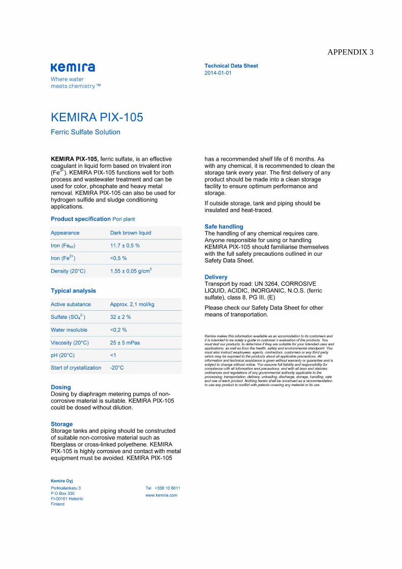
APPENDIX 3

APPENDIX 4

optimization of coagulant and coagulant aid in …

Documents