optimization of dose schedules in radiotherapy · optimization of dose schedules in radiotherapy by...
TRANSCRIPT

Optimization of dose schedules in radiotherapy
by
Pierre Miasnikof
A thesis submitted in conformity with the requirementsfor the degree of Master of Applied Science
Graduate Department of Mechanical and Industrial EngineeringUniversity of Toronto
Copyright c© 2013 by Pierre Miasnikof

Abstract
Optimization of dose schedules in radiotherapy
Pierre Miasnikof
Master of Applied Science
Graduate Department of Mechanical and Industrial Engineering
University of Toronto
2013
Purpose: Fractionation in radiotherapy is the scheduled break up of a total treatment
dose into individual doses. The goal of this thesis is to seek a mathematically optimal dose
schedule, in the context of a biological tissue dose-response model, the linear-quadratic
function.
Methods: We examined the mathematical properties of the fractionation problem in
the context of an arbitrary number of sensitive-structure constraints and determined the
properties of the optima. We also implemented a numerical search technique to solve the
problem.
Results: On the theoretical side, we confirmed and extended the results in the literature.
We showed the optima always occur at the intersection of two or more constraints or at
the equal dose per fraction point (or at any arbitrary feasible point on the boundary,
which includes the two points just mentioned). On the numerical side, we successfully
implemented a simulated annealing algorithm to our problem
ii

Acknowledgements
I would like to begin by expressing my deep gratitude to Doctor Harald Keller, my co-
supervisor. Dr. Keller is a practicing medical physicist at the Princess Margaret Hospital
and a professor in the Radiation Oncology Department of the Faculty of Medicine at the
University of Toronto. He provided me with a research topic and his work on fractiona-
tion formed the foundation for this thesis. I must also highlight Dr. Keller’s commitment,
generous sharing of expertise on the topic, scientific guidance, continuous feedback, sup-
port and warm encouragements, throughout this research endeavor. Without him, this
thesis would not have been possible.
I thank my supervisor, Professor Dionne Aleman who welcomed me into her lab, provided
direction, guidance, feedback and carefully reviewed the contents of this thesis. I also
thank the members of the committee, Professor Michael Carter and Professor Timothy
C. Y. Chan of the Mechanical and Industrial Engineering Department, for taking the
time to review my work and for their helpful comments.
Professor Matt Davison of the Applied Mathematics Department of the University of
Western Ontario provided helpful comments and shared his expertise on this topic, on
many occasions.
Special thanks go to Dominic Dotterrer of the Mathematics Department at the Univer-
sity of Toronto. Dominic’s advice on the geometry of the fractionation problem and
suggestions regarding the change of coordinate system were invaluable and necessary for
the completion of this thesis and derivation of theoretical results.
All errors, typos, inaccuracies are entirely mine.
iii

Contents
1 Introduction 1
1.1 Organization . . . . . . . . . . . . . . . . . . . . . . . . . . . . . . . . . 2
1.2 Contribution . . . . . . . . . . . . . . . . . . . . . . . . . . . . . . . . . . 3
2 Literature review 4
2.1 Dose fractionation in radiotherapy . . . . . . . . . . . . . . . . . . . . . . 4
2.2 Global optimization search techniques . . . . . . . . . . . . . . . . . . . . 10
3 The fractionation problem 17
4 Traditional mathematical programming approach 23
4.1 The Karush-Kuhn-Tucker conditions . . . . . . . . . . . . . . . . . . . . 24
4.2 First-order enumeration . . . . . . . . . . . . . . . . . . . . . . . . . . . 28
4.3 Convex maximization, a counter-example . . . . . . . . . . . . . . . . . . 29
5 Properties of the fractionation problem 33
5.1 Known analytic optima . . . . . . . . . . . . . . . . . . . . . . . . . . . . 33
5.2 Change of coordinates . . . . . . . . . . . . . . . . . . . . . . . . . . . . 37
5.3 Generalized properties of the optima . . . . . . . . . . . . . . . . . . . . 40
6 Simulated annealing 48
iv

7 Numerical results 54
7.1 Benchmark cases . . . . . . . . . . . . . . . . . . . . . . . . . . . . . . . 55
7.2 Comparison of interior and boundary search algorithms . . . . . . . . . . 56
7.3 Parameter selection and solution quality . . . . . . . . . . . . . . . . . . 58
7.4 Single tumor, single sensitive structure case . . . . . . . . . . . . . . . . 64
7.5 Multiple sensitive structures case . . . . . . . . . . . . . . . . . . . . . . 66
7.6 Time-varying radiosensitivity parameters . . . . . . . . . . . . . . . . . . 69
8 Discussion and conclusions 74
8.1 Summary . . . . . . . . . . . . . . . . . . . . . . . . . . . . . . . . . . . 74
8.2 Suggestion for future work . . . . . . . . . . . . . . . . . . . . . . . . . . 75
A Alternate solution techniques investigated 77
A.1 Steepest descent/ascent . . . . . . . . . . . . . . . . . . . . . . . . . . . . 77
A.2 Non-linear projected gradient . . . . . . . . . . . . . . . . . . . . . . . . 78
Bibliography 79
v

List of Tables
7.1 EQDF treatment benchmark test case, αT
βT> αS
ωβS. . . . . . . . . . . . . . 55
7.2 Single-dose treatment benchmark test case, αT
βT< αS
ωβS. . . . . . . . . . . 56
7.3 Mean percent deviation from analytic solution of objective function yielded
by regular and boundary search algorithms . . . . . . . . . . . . . . . . . 58
7.4 Two-sample t-test, null hypothesis of equal means, regardless of starting
point . . . . . . . . . . . . . . . . . . . . . . . . . . . . . . . . . . . . . . 63
7.5 Solution accuracy measured with respect to known optimum . . . . . . . 66
7.6 Numerical results, multiple constraint EQDF cases, second constraint dom-
inates. BFSD denotes the value of the objective at the best feasible single-
dose solution given the set of constraints and BFEQDF denotes the value
of the objective at the best feasible equal-dose solution given the same set
of constraints . . . . . . . . . . . . . . . . . . . . . . . . . . . . . . . . . 68
7.7 Numerical results, multiple constraint EQDF cases, seventh constraint
dominates. BFSD denotes the value of the objective at the best feasi-
ble single-dose solution given the set of constraints and BFEQDF denotes
the value of the objective at the best feasible equal-dose solution given the
same set of constraints . . . . . . . . . . . . . . . . . . . . . . . . . . . . 70
vi

7.8 Numerical results, shifting dominant constraint, single-dose cases, second
then twelfth constraint dominate respectively. BFSD denotes the value
of the objective at the best feasible single-dose solution given the set of
constraints and BFEQDF denotes the value of the objective at the best
feasible equal-dose solution given the same set of constraints . . . . . . . 71
7.9 Numerical results, multiple dominant constraints, EQDF case. BFSD de-
notes the value of the objective at the best feasible single-dose solution
given the set of constraints and BFEQDF denotes the value of the objec-
tive at the best feasible equal-dose solution given the same set of constraints 72
vii

List of Figures
3.1 Contours of two different linear-quadratic functions, circles centered in the
third quadrant, in a two-fraction case (R2) . . . . . . . . . . . . . . . . . 19
3.2 (a) Feasible set with more than one sensitive structure LQ constraint, with
one dominant constraint (in blue) and (b) dominant constraints intersect-
ing at arbitrary points (also in blue) . . . . . . . . . . . . . . . . . . . . 21
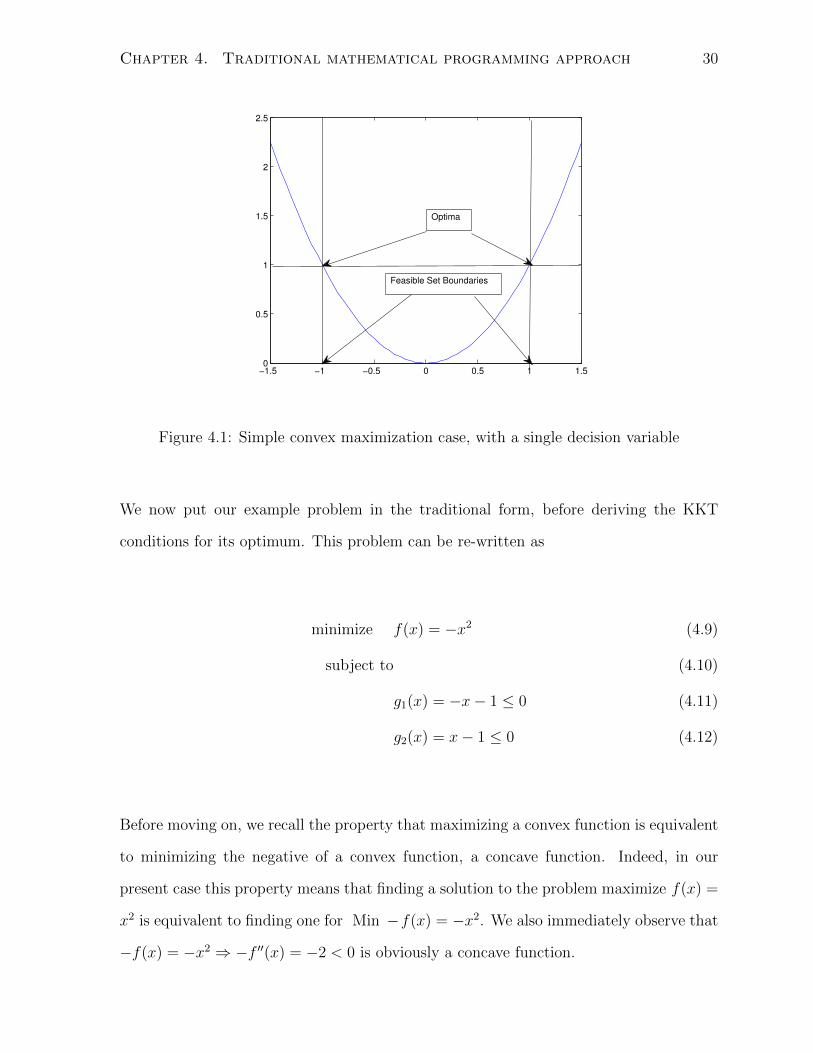
4.1 Simple convex maximization case, with a single decision variable . . . . . 30
5.1 Two possible optimal solutions in the single sensitive structure constraint
case, (a) the single dose treatment and (b) the equal dose per fraction
treatment . . . . . . . . . . . . . . . . . . . . . . . . . . . . . . . . . . . 36
5.2 Change of coordinates example in R2 . . . . . . . . . . . . . . . . . . . . 39
6.1 Penalty scheme on interior and exterior of the feasible set . . . . . . . . . 51
7.1 Dose per fraction versus known optimal dose, regular and boundary algo-
rithms (single sensitive structure constraint) . . . . . . . . . . . . . . . . 57
7.2 Effect of initial temperature (T0) on mean percent divergence from known
optimum (δ) . . . . . . . . . . . . . . . . . . . . . . . . . . . . . . . . . . 59
7.3 Effect of search radius (r) on mean percent divergence from known opti-
mum (δ) . . . . . . . . . . . . . . . . . . . . . . . . . . . . . . . . . . . . 60
viii

7.4 Effect of penalty coefficient (P ) on mean percent divergence from known
optimum (δ) . . . . . . . . . . . . . . . . . . . . . . . . . . . . . . . . . . 61
7.5 Effect of number of iterations (N) on mean percent divergence from known
optimum (δ) . . . . . . . . . . . . . . . . . . . . . . . . . . . . . . . . . . 62
7.6 Comparison of simulated annealing dose per fraction and known optimal
dose . . . . . . . . . . . . . . . . . . . . . . . . . . . . . . . . . . . . . . 65
7.7 Doses per fraction with time varying radiosensitivity parameters, start-end
trend line in black . . . . . . . . . . . . . . . . . . . . . . . . . . . . . . . 73
ix

Chapter 1
Introduction
Every day, clinical practitioners involved in radiation therapy treatments must decide
how to best divide a global treatment dose into a number of fractional dose increments.
In doing so, they must balance the need to destroy tumor cells with the need to preserve
healthy sensitive structures which also receive radiation, during treatment. Currently,
there are no formal universally accepted benchmarks for doing fractionation and dose-
scheduling is left to the discretion of the practitioner. In the past, fractionation of
treatment was the subject of much debate, but in recent practice fractionation schedules
are mostly developed by trial and error and are often defined by consensus. In clinical
practice, typical radiotherapy treatments involve the total prescription dose being broken
up either into 35 to 40 fractions of equal doses or in a few (one to three, generally) fractions
with large doses (e.g., radiosurgery treatment).
During the last decade however, novel technology allowed patients to be treated much
more precisely than in the past. Patient setup can now be monitored and corrected daily
and dose distributions can be made to conform very closely to the shape of the target.
At the same time, these advances allow better sparing of normal tissues and have revived
1
Chapter 1. Introduction 2
an old debate on fractionation.
In this thesis, we aim to mathematically derive the optimal dose per fraction, which
maximizes tumor cell kill while keeping the effects of dosage to heathy structures below
a predetermined level. We use the yet to be published work of Keller and Davison (2008)
and the work of Mizuta et al. (2012) as a methodological basis for our formulation.
1.1 Organization
We begin by briefly reviewing the history of radiotherapy fractionation, the radiobiologi-
cal basis for fractionation, including the widely used linear-quadratic model, and attempts
at formally arriving at an optimal fractionation scheme. We also examine different global
optimization search algorithms as possible tools for solving difficult optimization prob-
lems, in general, and our specific fractionation problem, in particular. We then pose the
fractionation problem as it exists currently in the literature and attempt to generalize its
formulation, while examining the mathematical properties of the optima. In the course of
doing so, we demonstrate why traditional mathematical programming techniques do not
apply to our specific problem and why numerical search techniques, specifically simulated
annealing, are required to attain a numerical solution.
Finally, we explore various simulated annealing parameter settings and tailor a simulated
annealing algorithm that best suits our particular problem. We apply our algorithm on
a set of sample cases to assess solution quality and explore actual dosage results.

Chapter 1. Introduction 3
1.2 Contribution
In the most recent literature, the fractionation problem is formulated in the context of a
dosage delivered to a tumor, constrained by a single healthy structure adversely affected
by this dose and a tumor with constant sensitivity to radiation. We aim to generalize
this problem formulation to a more realistic case where the doses delivered to the tumor
are constrained by a finite arbitrary number of healthy structures and where the tumor’s
radiosensitivity may evolve over the course of the treatment.
A numerical search algorithm was also developed to solve this more generalized formula-
tion and to find solutions in the case where the tumor’s reaction to radiation may evolve
over the course of treatment.
Finally, a clarification to the theorem presented in Keller and Davison (2008) and a
generalization of it to the case of an arbitrary number of healthy structures that impose
dosage constraints are offered.

Chapter 2
Literature review
2.1 Dose fractionation in radiotherapy
Fractionation, the scheduled break-up of a radiotherapy treatment into a set of treatment
increments, has a long history dating back to the 19th century. Thames (1992) lays out
a detailed history of fractionated radiation treatment, going back to the 1890’s. In 1896,
a physician by the name of Leopold Freund treated a patient afflicted with a hairy
nevus by administering a low daily dose of X-rays, over two weeks. At about the same
time, in Sweden, Thor Stenbeck reported using a similar technique to treat cases of
skin cancer. Unfortunately, the actual doses delivered were unknown, due to a lack of
adequate dosimetric technology at the time.
Around 1902, beginning with the work of Holzknecht and later around 1909 with the work
of Villard, the technology to accurately measure the doses delivered began to appear. This
new technology not only allowed therapists to measure dose, but provided them with the
ability to deliver higher doses in fewer sessions. Thus was born the fractionation debate.
Indeed, throughout the 20th century, a persistent debate over the relative merits of large
4
Chapter 2. Literature review 5
doses over fewer fractions versus smaller doses over longer treatments endured. This
debate perdured, even if each school of thought claimed its approach to be rooted in
human biology (Miles and Lee, 2008).
To this day, the debate remains, in spite of the tremendous advancements in radiotherapy
we have witnessed since this debate began. Although fractionation (as opposed to single
treatment) seems to be the dominant school of thought, no consensus exists on the
precise manner in which dosage should be administered. For example, Miles and Lee
(2008) claim hypofractionation, a shortened higher dose per fraction treatment, may be
advantageous in some prostate cases. As recently as 2010, Ferreira et al. (2010) conducted
a retrospective evaluation of different IMRT fractionation schedules of head and neck
tumors to assess their comparative advantages. Even if their study seems to suggest
shorter higher dose per fraction treatments yield better tumor control probabilities, their
results remain preliminary and are based on a very small sample size (seven patients).
In the late 20th and early 21st century, some work focuses on building a formal radiobi-
ological framework for evaluating the effects of fractionation. Fowler (1989) reviews the
link between treatment time, tissue and tumor biology, on the one hand, and the efficacy
of treatment schedules, on the other. He links fractionation schedules that account for
radiobiological factors such as dose-delivery over time and the role they play in the clin-
ical success of a treatment. He also mentions that early, but not late, adverse reactions
can be reduced or eliminated by extending treatment times.
Later, in Fowler (1992), the author updates and adds to his previous work. He also
summarizes the main facets of the radiobiological basis for fractionated treatment and
identifies the following important facts:
• Late and early complications in normal tissue are made worse by large doses per
fraction;
Chapter 2. Literature review 6
• 2 Gy per fraction will sterilize approximately half the cells in most tumors;
• The effect of radiation damage can be assessed using an existing model (linear-
quadratic model).
Lee et al. (1998) examine the effects of treatment duration, total treatment dose and
fractionation on post-treatment cerebral necrosis. They found the fractionation scheme
to be the most determining factor in predicting post-treatment cerebral necrosis. For
example, in a sample of over 1,000 patients suffering from nasopharyngeal carcinoma,
they found that patients who received 60 Gy in total in 2.5 Gy fractional increments had
lower rates of temporal lobe necrosis than those who received a total dose of 50.4 Gy in
4.2 Gy increments.
Mavroidis et al. (2001) develop the concept of biologically effective uniform dose, an as-
sumption that two dose distributions are equivalent if they achieve similar tumor control
probabilities. Nevertheless, despite this biological equivalence, they insist that one needs
to account for the fractionation schedule when comparing treatments. They claim that
the dose-response parameters of the tissues depend on how the treatment was delivered.
Bourhis et al. (2006) conduct a meta-analysis of accelerated and hyperfractionated ra-
diotherapy treatment of head and neck cancer. They analyze 15 trials with over 6,500
patients and conclude that in comparison to conventional radiotherapy both accelerated
treatments (shorter higher dose per fraction) and hyperfractionated treatments (multiple
treatments per day) lead to greater tumor control probabilities. They also conclude that
hyperfractionated treatment schedules provide the greatest benefit.
Ma et al. (2010) study equivalent uniform biologic effective dose (EUBED) on normal
brain tissue under different fractionation schemes (1-30 fractions) for three different treat-
ment modalities (Gamma Knife, Cyberknife and a Novalis LINAC-based system). They
find that according to the tumor’s radiosensitivity characteristics the fractionation sched-

Chapter 2. Literature review 7
ule is a significant factor in determining normal tissue sparing, regardless of the treatment
modality.
To model the effects of radiation on the tissues, the linear-quadratic model was developed
in the early 1980’s. Since then, it has held up well in the face of empirical validation
(Fowler, 1989) and seems to be, to this day, the most widely employed model for predict-
ing the dose-time relationship and evaluating the effect of different dose-per-fractionation
schedules (Brenner, 2008).
Many authors have made use of and modified the linear-quadratic model, to achieve
various goals (Brenner et al., 1998; Yang and Xing, 2005; Keller and Davison, 2008;
Mizuta et al., 2012), but they all share a common model core. At its core, the linear-
quadratic model describes what is referred to as the radiobiological effect E, as a second
degree polynomial function called the linear-quadratic (LQ) function of the total dose d
delivered to tissues over the course of a treatment.
E = αd+ βd2
The coefficients α, β are referred to as the radiosensitivity parameters or radiosensitivity
coefficients of a given tissue structure. In a mechanistic interpretation, these parameters
describe different damage to the cell’s DNA. Naturally, both these coefficients are positive,
since a radiation dose must have some tissue damage effect. A negative coefficient would
imply an inverse relationship between dose and cell death (more dose, less cell damage).
The cell kill (CK) caused by a radiation treatment is the exponential of the effect E:
CK = exp (E) = exp(αd+ βd2)
According to Fowler (1992) the dose effect is additive over multiple fractions, in the
linear-quadratic model. Therefore, the total effect over the course of a treatment of N
Chapter 2. Literature review 8
fractions can be expressed as
E = α
N∑i=1
di + β
N∑i=1
d2i
Conversely, using this model, we can also evaluate a cell’s survival fraction (SF) over the
course of a treatment as a function of the doses received in each fraction:
SF = exp(−E) = exp
(−α
N∑i=1
di − βN∑i=1
d2i
)For the purpose of predicting the effects of radiation on tumor and normal tissues, the
linear-quadratic model has been evaluated rigorously. It was found to be accurate, robust,
based on solid theoretical foundations and submitted to empirical validation (Fowler,
1989; Brenner et al., 1998; Brenner, 2008) for typical dose ranges.
The linear-quadratic model does have its limitations, nonetheless, and is still the subject
of much debate. Although it can reliably be applied to doses in the range of 2-10 Gy per
fraction, it becomes less accurate at higher doses, in the 15-18 Gy range (Brenner, 2008),
and is found to be inaccurate for the larger doses required in radiosurgery (Kirkpatrick
et al., 2008).
While the use of mathematical optimization to formally determine a treatment plan’s
overall beam-dosage in radiotherapy has been addressed by a very large number of au-
thors, very few papers address the specific problem of determining the optimal dose for
each fraction. For example, Romeijn et al. (2006) consider the problem of designing a
fraction within a treatment plan, with known and pre-determined beam orientations, by
computing the optimal beamlet weights. Chu et al. (2005); Chan et al. (2006) focus on
optimizing a fraction under uncertainty due to motion. Unfortunately, not a lot of work
has been done to examine the optimal delivery schedule of the dose over the course of
the entire multi-fraction treatment.
Only a few publications to date attempt to solve the specific problem of determining the
optimal dose for each fraction. Levin-Plotnik and Hamilton (2004) consider a tumor’s

Chapter 2. Literature review 9
tissue density to find the dose schedule that maximizes tumor-control probability (TCP)
for a fixed mean-dose per fraction (i.e., a fixed total treatment dose). They conclude that
for homogeneous cell densities a homogeneous dose schedule maximizes the TCP, while
for heterogeneous tumor density they conclude an initial inhomogeneous dose will homog-
enize the tumor density and all subsequent doses can then be homogeneous. Yang and
Xing (2005) use the linear-quadratic model to develop a “tumor-biology specific” dose-
schedule that maximizes the tumor’s biologically effective dose (BED), while keeping the
heathy structure’s BED constants. Their problem formulation involves only constraints
from a single sensitive structure and fractional dose constraints. Aleman et al. (2007)
integrate the time dimension within the IMRT plan optimization by taking a physical
view of the problem and solving for the individual beamlet weights in each fraction of the
treatment. Hoffmann et al. (2008) address the fractionation effect on tumor-control and
normal-tissue complication probabilities, but do not address the problem of determining
the optimal dose per fraction.
In a different problem formulation, Keller and Davison (2008); Mizuta et al. (2012) com-
pute instead the optimal dose per fraction, for the case of a single tumor and single sen-
sitive structure constraint, within the framework of a time-independent linear-quadratic
model, without imposing any fractional dose constraintsl. Keller and Davison (2008)
solve the optimal fractionation problem through dynamic programming and by the for-
mulation of a theorem. Their theorem identifies two possible optimal schedule cases, the
single-dose treatment schedule, in which the entire treatment dose is delivered in a single
fraction, and the equal dose per fraction treatment schedule (EQDF), in which the treat-
ment is broken down into fractions of equal dose. The optimality of each dose-schedule
depends on the alpha-beta ratio of the the tumor and sensitive structure linear-quadratic
functions. Without resorting to dynamic programming to validate their claims numeri-
cally, Mizuta et al. (2012) come to the same conclusions. This framework was recently
applied to more general sensitive tissue constraint functions, such as a normal-tissue
Chapter 2. Literature review 10
complication probability (NTCP) model (Keller et al., 2012).
The bulk of the work presented in this document focuses on suggesting alternative solu-
tion approaches to the optimization problem posed in Keller and Davison (2008) and in
generalizing it to the multiple-tumor and multiple-sensitive structure case.
2.2 Global optimization search techniques
Later in this thesis we will show that traditional mathematical programming techniques
do not apply to our specific fractionation problem. For this reason, we explored global
optimization techniques.
When it is hard or impossible to obtain analytical solutions to an optimization problem,
there exists a vast array of global optimization search techniques to approximate a glob-
ally optimal solution. While each of these techniques has its own specificities, they all
explore the feasible set of a problem in a systematic manner, typically without relying on
the objective function’s derivative. We briefly reviewed five common techniques, random
search, tabu search, genetic algorithms, GRASP and simulated annealing, to assess their
suitability for our problem. We also examined the extensive applications of simulated
annealing in the medical physics literature and to radiotherapy problems, in particular.
Random search is a global optimization algorithm that consists of exploring the feasible
set randomly, by following a uniform probability, and retaining the best solution (Brown-
lee, 2011). The biggest shortcoming of random search is that it is a memoryless search,
which may revisit points in the feasible set. Because of this feature of the search strategy,
in the worst-case, performance may be worse than complete enumeration, since the same
points may be visited more than once. In spite of this worst-case behavior, random search
has been found to be an acceptable solution tool for some mixed-integer problems (Nelson

Chapter 2. Literature review 11
and Brodie, 1990). On the other hand, Westhead et al. (1997) compared performances
of random search, tabu search, genetic algorithms, evolutionary programming (another
search technique) and simulated annealing, on a molecular-docking problem, and found
random search provided the worst performance of all techniques. Most applications of
random search typically involve unconstrained problems, but they have also been success-
fully applied to constrained problems, as well (Solis and Wets, 1981; Niemierko, 1992).
Notably, Niemierko (1992); Niemierko et al. (1992) used random search to solve a con-
strained beam weight selection problem. They reported clinically valid, although not
provably optimal, solutions within a few minutes of runtime.
Tabu search is a “meta-heuristic” algorithm, a heuristic algorithm applied on top of an-
other heuristic algorithm. It is typically overlaid on another search technique, such as a
traditional hill-climbing algorithm, for example (Brownlee, 2011). It enhances the search
by ensuring that recently visited points are not revisited before some time has passed, by
maintaining a “tabu list”. The tabu list addresses the shortcomings of the random search
technique, just described (Brownlee, 2011). Westhead et al. (1997), in their comparisons
of search techniques on a molecular-docking problem, reported tabu search returned rea-
sonable and comparable results with most of the other search techniques they considered,
although it was found to be clearly superior to the random search technique. Kapamara
et al. (2006) found tabu search outperformed other search techniques on job-shop prob-
lems. While tabu search was developed initially for combinatorial problems, it has also
been applied to continuous ones (Chelouah and Siarry, 2000). In fact, it was success-
fully applied to various problem formulations in conformal radiotherapy, including beam
weight selection, number of beams, beam direction (Gilio, 1997).
Genetic algorithms fall into the category of evolution-inspired algorithms that mimic
biological processes and which are broadly categorized as evolutionary algorithms. These
algorithms explore the solution space by creating a population of candidate solutions

Chapter 2. Literature review 12
and combining these candidates, in order to obtain a better solution, thus mimicking
genetic mechanisms (Michalewicz, 1995; Brownlee, 2011). Points in the feasible space are
encoded as binary strings. The most promising points are combined to form new points,
which is where they get their name. The general assumption is that by combining the
characteristics of promising points in the feasible set we get points that represent better
solutions. In their comparisons, Westhead et al. (1997) found genetic algorithms to
perform similarly to most of the other techniques they examined. In the past, genetic
algorithms have been used to solve (photon) beam selection problems in radiation therapy
within clinically acceptable time frames (Ezzell, 1996; Li et al., 2004) More recently, Cao
et al. (2012) also obtained good results with proton beam problems.
Greedy randomized adaptive search procedure (GRASP) is a commonly used meta-
heuristic technique in combinatorial optimization. For example, Petrovic and Leite-
Rocha (2008) applied this technique to a radiotherapy appointment scheduling problem.
GRASP is a combination of greedy search and local search techniques. It begins by
selecting a set of candidate points, and then applying a greedy search. Greedy search
is a short-sighted search strategy that moves from point to point by selecting the point
which provides the highest payoff among possible moves. The GRASP procedure then
applies local search, a series small perturbations on the candidates points obtained by
greedy search, to explore possible improvements upon these candidate solutions (Hirsch
et al., 2007; Brownlee, 2011). Although used primarily for combinatorial problems, this
method has also been applied to continuous problems (Hirsch et al., 2007).
Simulated annealing (Bertsimas and Tsitsiklis, 1993; Russell and Norvig, 1995; Brownlee,
2011) is a well-known global optimization technique. It is a variant of “hill-climbing”
that does not systematically apply a greedy logic to determine a move from the current
point to the next point. In simulated annealing, we search the feasible set by moving
from a current point to a new point according to the following set of search rules. If
Chapter 2. Literature review 13
the new point in our search improves the objective function the move is automatically
accepted. In the case where the new point does not improve the objective function, it
is accepted if a random draw is lower than an evolving probability of acceptance. This
acceptance procedure allows simulated annealing to break out of local optima.
Most of the simulated annealing literature is illustrated with basic unconstrained com-
binatorial problems. However, many authors (Morrill et al., 1991; Romeijn and Smith,
1994; Wah and Wang, 1999; Wah and Chen, 2000; Miki et al., 2006) have successfully
applied simulated annealing to continuous and constrained problems.
Simulated annealing is very commonly used in the medical physics literature. Although
no theoretical justification is made for this choice of solution technique, good numerical
results have been reported. In the past, it has been applied to solve various radiother-
apy problems. For example Webb (1989); Mageras and Mohan (1993) used simulated
annealing to determine beam weights. Morrill et al. (1991); Aleman et al. (2008) used
simulated annealing to determine beam angles and weights and reported reasonable run
times. Bortfeld and Schlegel (1993) showed the need for search techniques to solve non-
convex problems and then applied simulated annealing to a beam orientation problem.
Cao et al. (2012) used simulated annealing and genetic algorithms as benchmarks to
compare their own solution technique for a beam angle optimization problem. Simulated
annealing techniques have also been applied to a (different from ours) formulation of the
dose fractionation problem (Yang and Xing, 2005).
Westhead et al. (1997), in their comparison of various search algorithms, found the nu-
merical performance of all the techniques to be roughly equivalent, except for random
search which they found inferior to the other techniques they considered. Rossi-Doria
et al. (2003) compared the performance of different metaheuristics on various instances of
a timetabling problem. The metaheuristic techniques they compared were evolutionary
algorithms, ant colony optimization, iterated local search, simulated annealing, and tabu
Chapter 2. Literature review 14
search. In the end, they concluded that it was impossible to determine which technique
would offer the best performance for all instances of their benchmark problem. Kapamara
et al. (2006) compared various search techniques on a scheduling problem. They com-
pared the performance of branch-and-bound, simulated annealing, tabu search, GRASP
and genetic algorithms and found tabu search outperformed the other techniques. In
another comparative study, Perez and Basterrechea (2007) examined the performance of
variations of genetic algorithms, simulated annealing and particle swarm optimization,
on antenna measurement problems. They found that particle swarm optimization and
simulated annealing techniques were the best suited to their problems. Cao et al. (2012)
also compared the performance of various search techniques in the solution of a beam
angle problem and found no significant differences in the performance.
Finally, in order to put the conclusions of Westhead et al. (1997); Rossi-Doria et al.
(2003); Perez and Basterrechea (2007); Cao et al. (2012) in proper context, it is impor-
tant to mention that all global optimization search algorithms have their strengths and
weaknesses. At present, no algorithm has been found to be generally superior or even su-
perior for a specific class of problems. Some algorithms perform better on some particular
problems, while other algorithms perform better on other specific problems. This char-
acteristic is known as the “no free lunch” property of search algorithms in optimization
(Wolpert and Macready, 1997; Brownlee, 2011, p. 14).
In summary, while it is virtually impossible to select the “best” global optimization search
techniques for all cases, it may be useful to remember the following characteristics:
• Random search
– Cycling possible
– May get caught in local optimum

Chapter 2. Literature review 15
– Bad worst-case behavior
• Tabu search
– Avoids cycling, by maintaining tabu list
– Maintenance of tabu list may impose computational overhead, especially when
decision variables are multi-dimensional
– Tabu is generally overlaid on a hill-climbing heuristic, which may get stuck in
local optima
• Genetic algorithms
– Rely on the assumption that combining good points of the feasible space will
lead to better ones
– As a result, may get caught in local optima
• GRASP
– Combines greedy search and local search heuristics
– Both are susceptible to getting stuck in local optima
• Simulated annealing
– Known to converge to global optimum asymptotically
– Able to break out of local optima, so it is well suited when the shape of the
search space is unknown or hard to predict
– Widely used in the medical physics literature, e.g., previously used for IMRT
optimization and fractionation

Chapter 2. Literature review 16
Because of its previous use in the medical physics literature and convergence properties,
simulated annealing was the numerical technique of choice for this thesis.
Chapter 3
The fractionation problem
We begin this chapter by introducing the base case of single tumor and single sensitive
structure problem posed by Keller and Davison (2008); Mizuta et al. (2012), which is
the most current version of the fractionation optimization problem. We then generalize
this problem to the more realistic case of a treatment constrained by multiple sensitive
structures and the case of time-dependent radiosensitivity parameters.
In the literature, the most current formulation of the fractionation problem is a problem
in which we seek the dose per fraction schedule that maximizes the effect of radiation
on a tumor, thus also maximizing a tumor’s cell kill, while keeping the effect (and cell
kill) imposed on a single sensitive structure to a predetermined level, for a treatment of
known length (known number of fractions) N (Keller and Davison, 2008; Mizuta et al.,
2012). Note here that if a fractional dose di is equal to zero, the number of fractions
where dose is actually being delivered is less than N . In that sense, N is an upper bound
for the number of fractions in which dose is delivered.
For both the tumor and sensitive structure cell kill is given by the linear-quadratic model.
For mathematical clarity and numerical stability, these authors work with the LQ func-
17

Chapter 3. The fractionation problem 18
tion, the natural logarithm of the cells’ cell kill function, the effects function seen in
Section 2.1. For a treatment of N fractions, the problem is expressed as follows (Keller
and Davison, 2008; Mizuta et al., 2012):
maximize f(~d) =N∑f=1
(αTdf + βTd
2f
)(3.1)
subject to (3.2)
g(~d) =N∑f=1
(αSωdf + βSω
2d2f
)= K (3.3)
df ≥ 0 ∀f = 1, . . . , N (3.4)
The parameter ω(≥ 0) is the “sparing factor” of the sensitive structure. It indicates the
amount of radiation, ωdi, that is delivered to the sensitive structure when the adjacent
tumor is administered a radiation dose di.
Before moving forward, we must mention that the linear-quadratic model with constant
positive parameters has two important mathematical properties with respect to the frac-
tional doses. Keller and Davison (2008) describe these properties in detail and exploit
them in their work. First, the order of the doses does not matter. Two dose regimens
with the same overall dosage breakdowns have the same effect, regardless of the dose
ordering in time, for example, α(d1 + d2) + β(d21 + d2
2) = α(d2 + d1) + β(d22 + d2
1). Second,
the quadratic term gives higher weight to large fractional doses, regardless of the total
dose. For example, we have α(5 + 5) +β(52 + 52) ≤ α(10 + 0) +β(102 + 0), with α, β ≥ 0.
Although we used a simple two-fraction example to illustrate these properties, they hold
for any arbitrary number of fractions and any arbitrary permutation of the doses.
Finally, it should be noted the set of vectors of doses ~d = [d1 . . . dN ]T satisfying linear-
quadratic equation α∑N
f=1 df + β∑N
f=1 d2f = K defines an N -dimensional hypersphere
centered at the point [−α/(2β) . . .−α/(2β)]T and having a radius of√
Kβ
+N (α/(2β))2,
as described in Mizuta et al. (2012).
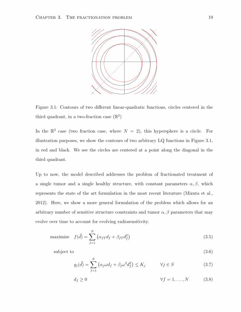
Chapter 3. The fractionation problem 19
Figure 3.1: Contours of two different linear-quadratic functions, circles centered in the
third quadrant, in a two-fraction case (R2)
In the R2 case (two fraction case, where N = 2), this hypersphere is a circle. For
illustration purposes, we show the contours of two arbitrary LQ functions in Figure 3.1,
in red and black. We see the circles are centered at a point along the diagonal in the
third quadrant.
Up to now, the model described addresses the problem of fractionated treatment of
a single tumor and a single healthy structure, with constant parameters α, β, which
represents the state of the art formulation in the most recent literature (Mizuta et al.,
2012). Here, we show a more general formulation of the problem which allows for an
arbitrary number of sensitive structure constraints and tumor α, β parameters that may
evolve over time to account for evolving radiosensitivity.
maximize f(~d) =N∑f=1
(αfTdf + βfTd
2f
)(3.5)
subject to (3.6)
gj(~d) =N∑f=1
(αjωdf + βjω
2d2f
)≤ Kj ∀j ∈ S (3.7)
df ≥ 0 ∀f = 1, . . . , N (3.8)
Chapter 3. The fractionation problem 20
In this case, we are still maximizing the cell kill of tumor cells, but are now restricted by a
set S of multiple sensitive-structures, indexed by the subscript j. Note that the equality
constraint in equation 3.3 has been replaced by a set of inequalities, in statement 3.7. This
replacement ensures that we do not end up with an empty feasible set, due to inconsistent
restrictions on the dosage, which may be imposed by the the multiple sensitive-structure
constraints. Indeed, some sensitive-structures may impose greater restrictions on the
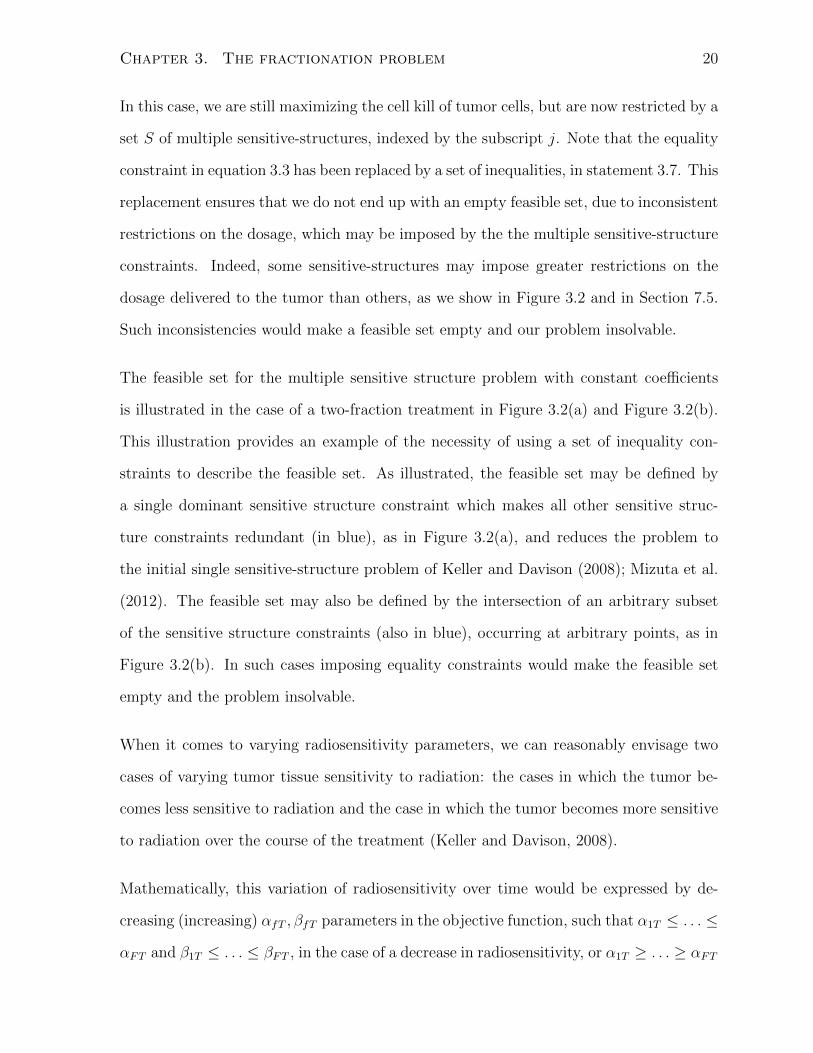
dosage delivered to the tumor than others, as we show in Figure 3.2 and in Section 7.5.
Such inconsistencies would make a feasible set empty and our problem insolvable.
The feasible set for the multiple sensitive structure problem with constant coefficients
is illustrated in the case of a two-fraction treatment in Figure 3.2(a) and Figure 3.2(b).
This illustration provides an example of the necessity of using a set of inequality con-
straints to describe the feasible set. As illustrated, the feasible set may be defined by
a single dominant sensitive structure constraint which makes all other sensitive struc-
ture constraints redundant (in blue), as in Figure 3.2(a), and reduces the problem to
the initial single sensitive-structure problem of Keller and Davison (2008); Mizuta et al.
(2012). The feasible set may also be defined by the intersection of an arbitrary subset
of the sensitive structure constraints (also in blue), occurring at arbitrary points, as in
Figure 3.2(b). In such cases imposing equality constraints would make the feasible set
empty and the problem insolvable.
When it comes to varying radiosensitivity parameters, we can reasonably envisage two
cases of varying tumor tissue sensitivity to radiation: the cases in which the tumor be-
comes less sensitive to radiation and the case in which the tumor becomes more sensitive
to radiation over the course of the treatment (Keller and Davison, 2008).
Mathematically, this variation of radiosensitivity over time would be expressed by de-
creasing (increasing) αfT , βfT parameters in the objective function, such that α1T ≤ . . . ≤
αFT and β1T ≤ . . . ≤ βFT , in the case of a decrease in radiosensitivity, or α1T ≥ . . . ≥ αFT

Chapter 3. The fractionation problem 21
(a) LQ constraints, multiple sensitive
structures, one dominant constraint
(b) LQ constraints, multiple sensitive
structures, arbitrarily intersecting con-
straints
Figure 3.2: (a) Feasible set with more than one sensitive structure LQ constraint, with
one dominant constraint (in blue) and (b) dominant constraints intersecting at arbitrary
points (also in blue)

Chapter 3. The fractionation problem 22
and β1T ≥ . . . ≥ βFT , in the case of an increase in radiosensitivity. Decreasing (increas-
ing) parameters means that for the same dose the effect on the tumor decreases (increases)
over time as parameter values evolve over the course of treatment. Our generalized for-
mulation now allows for time varying radiosensitivity coefficients αfT , βfT , which are
indexed for each of the f = 1, . . . , N fractions of the treatment.
In looking into the effect of time-varying radiosensitivity parameters, it is important
to recall the properties of the linear-quadratic function with constant parameters. As
described in Section 2.1, the order of the doses does not matter, and two dose schedules
with the same dosages have the same effect, regardless of how the doses are ordered in
time. However, by making the radiosensitivity parameters vary over the course of the
treatment, we break this property.

Chapter 4
Traditional mathematical
programming approach
Before moving forward with our problem formulation, it is important to demonstrate
that the commonly used Karush-Kuhn-Tucker (KKT) conditions for solving non-linear
optimization problems are not helpful in the case of our fractionation problem.
For the reader’s benefit, we restate the KKT conditions for a general case. We then show
a simple counter-example that illustrates our claim and then use our actual problem
formulation to show that KKT conditions do not apply in our specific case. We end this
chapter by justifying to the reader why a numerical search technique is required to solve
the fractionation problem.
23

Chapter 4. Traditional mathematical programming approach 24
4.1 The Karush-Kuhn-Tucker conditions
Prior to demonstrating the inapplicability of the KKT conditions we find it useful to
restate them, in the context of a general constrained nonlinear problem, as shown here:
minimize or maximize f(x)
subject to
gi(x) ≤ 0 ∀i = 1, . . . , I
hj(x) = 0 ∀j = 1, . . . , J
The KKT conditions are a set of necessary (feasibility, stationarity and complementary
slackness) and sufficient (convexity/concavity) conditions for an optimum in a nonlinear
optimization problem, like the one just stated.
The first-order KKT condition states that for a feasible point to be an optimum it must
be a stationary point. Stationarity means that at an optimum x∗, the gradient of the
Lagrangian function for the constrained problem must equal zero:
∇L(x∗, µ, λ) = ∇f(x∗) +I∑i=1
(µi∇gi(x∗)) +J∑j=1
(λj∇hj(x∗)) = ~0
Where the variables µi, λj are the dual variables for the inequality and equality con-
straints, respectively. Also note this formulation is flexible enough so that the elements
of the triplet x∗, µ, λ can each be scalars or vectors. Additionally, for a point to be
an optimum the dual variables µ, λ must fulfill the following conditions, known as the
“complementary slackness” conditions, at the point x∗:
µi gi(x∗) = 0 ∀i = 1, . . . , I
If the ith inequality constraint is tight at the point x∗, then the dual varible µi must be
positive (µi ≥ 0). Otherwise, if the ith inequality is not tight, then µi must equal zero
(µi = 0). For the equality constraints, the variables λj can be any arbitrary scalar.
Chapter 4. Traditional mathematical programming approach 25
Finally, the sufficient (but not necessary) condition relates to the geometry of the La-
grangian (i.e., the geometry of objective function and feasible set). It states that a point
x∗ is a local maximum (minimum), if, in addition to meeting the necessary conditions
stated previously, the Lagrangian is also concave (convex) in the neighborhood of that
point x∗. Convexity (concavity) is verified by examining the Hessian matrix of the La-
grangian at the point x∗. If the Hessian is negative-definite in the neighborhood of the
point x∗, the Lagrangian is locally concave and x∗ can be classified as a local maximum.
Conversely, if the Hessian is positive-definite the Lagrangian is concave and x∗ is a local
minimum. If the Hessian is indefinite, the second-order conditions are inconclusive.
We now derive the KKT conditions based on the original formulation of Keller and
Davison (2008). We use a two fraction case for illustration purposes, but our results hold
for any number of fractions. We recall the problem of determining the doses for two
fractions that maximize tumor cell kill under one constraint is expressed in the literature
(Keller and Davison, 2008; Mizuta et al., 2012) as
maximize f(~d) = αTd1 + βTd21 + αTd2 + βTd
22
subject to
g(~d) = αSωd1 + βSω2d2
1 + αSωd2 + βSω2d2
2 = K
h1(~d) = −d1 ≤ 0
h2(~d) = −d2 ≤ 0
Before looking into optimality conditions, we begin with the examination of a plot of the
linear-quadratic function in R2, shown in Figure 3.1, Figure 3.2(a) and Figure 3.2(b).
These figures visually confirm its convex shape.
In order to remain consistent with the bulk of the mathematical programming literature
we will work with the minimization formulation of this problem for the rest of this chapter,
i.e., minimizef(~d) =∑F
f=1
(−αdf − βd2
f
). In the case of our fractionation problem, the

Chapter 4. Traditional mathematical programming approach 26
first-order conditions for optimality at a point ~d∗ for a two-fraction example are
∇L(~d∗, λ, ~µ) = ∇f(~d∗) + λ∇g(~d∗) + µ1∇h1(~d∗) + µ2∇h2(~d∗) = ~0 (4.1) −αT − 2βTd∗1
−αT − 2βTd∗2
+ λ
αSω + 2βSω2d∗1
αSω + 2βSω2d∗2
+ µ1
−1
0
+ µ2
0
−1
= ~0 (4.2)
−αT − 2βTd∗1 + λαSω + 2λβSω
2d∗1 − µ1
−αT − 2βTd∗2 + λαSω + 2λβSω
2d∗2 − µ2
=
0
0
(4.3)
d∗1
d∗2
=
µ1−λαSω+αT
−2βT +2λβSω2
µ2−λαSω+αT
−2βT +2λβSω2
(4.4)
Recall that
αT , αS, βT , βS, ω > 0 (4.5)
d1, d2 ≥ 0 (4.6)
µ1, µ2 ≥ 0 (4.7)
di > 0⇒ µi = 0 ∀i = 1, 2 (4.8)
Inequalities 4.5 and 4.6 always hold, by design, in our model. Inequalities 4.7 and 4.8
are part of the KKT necessary complementary slackness conditions for an optimum.
The general KKT second-order condition for an optimum in our given fractionation
problem is that the Hessian matrix for the restricted Lagrangian
HL(~d) =
[∂L(~d)
∂di∂dj
]=
−2βT + 2λβSω
2 0
. . .
0 −2βT + 2λβSω2
� or ≺ 0
be positive-definite for a minimum or negative-definite for a maximum, at the critical
point ~d∗ that meets the necessary conditions. However, because we are minimizing, we
are only interested in the cases where the Hessian matrix is positive-definite.
We observe that the Hessian is diagonal and has constant values along its diagonal.
We also know the diagonal elements cannot equal zero because of the ratios we derived
Chapter 4. Traditional mathematical programming approach 27
through the first-order condition. This condition excludes the semi-definite case (i.e.,
diagonal elements or eigenvalues equal to zero). So the second-order conditions, together
with the ratios in the first-order conditions, tell us that for the point ~d∗ to be a minimum,
we require −2βT + 2λβSω2 > 0 or, more simply, −βT + λβSω
2 > 0.
Note, λ ∈ R is unrestricted. This absence of bounds means our Lagrangian’s convex-
ity depends on the values of λ (recall the model parameters βT , βS, ω ≥ 0 are known).
Depending on the values of λ, the inequality βT + λβSω2 > 0 may or may not hold.
Consequently, the restricted Lagrangian may or may not be convex. Therefore, any
point satisfying the second-order condition can only be classified as a local minimum
through the application of the KKT theorem. In addition, some points not satisfying
the second-order condition but satisfying the first-order necessary condition, points lying
in neighborhoods where the restricted Lagrangian function is non-convex, may also be
optima, as will be seen in our example in Section 4.3. Our problem involves the mini-
mization of a concave (maximization of a convex) objective function, a problem shown
to be ill-suited to the KKT theorem, as demonstrated by the second-order condition just
presented, so these facts must be kept in mind.
Mathematical evidence of the non-convexity of this problem is provided by the equality
constraint for the sensitive structure g(~d) = αSωd1+βSω2d2
1+αSωd2+βSω2d2
2 = K, which
defines a non-convex set and by the objective function (recall: f ′′(~d) = −2βT < 0), which
is not convex. This evidence of non-convexity eliminates the relevance of the second-order
conditions. To prove the assertion that the feasible set, defined by equality constraints,
is not convex, we take a single-fraction example and apply the properties of convex
combinations of feasible points. Letting x1 and x2 be two arbitrary feasible points (doses
for a single-fraction treatment), the following equations hold:
g(x1) = αSx1 + βSx21 = K
g(x2) = αSx2 + βSx22 = K
Chapter 4. Traditional mathematical programming approach 28
Now take the convex combination of the two feasible points, x3 = θx1 + (1− θ)x2, where
0 ≤ θ ≤ 1. Because the function g(x) is convex, by definition, we have the the following
inequality: g(x3) = αS(θx1 + (1 − θ)x2) + βS (θx1 + (1− θ)x2)2 ≤ K, which means the
convex combination x3 may not be part of the feasible set.
In order to prove that the function g(x) is convex, all we need to do is to examine
its second-derivative g′′(x), which is always positive, regardless of the values x, since
βS ≥ 0 ⇒ g′′(x) = 2βS ≥ 0. Also, if βS = 0 and therefore g′′(x) = 0, then the function
g(x) is linear, which is also a convex function.
In summary, we must remember the concave minimization problem (convex maximiza-
tion) is in fact a non-convex problem. The optima may lie on a convex segment of the
Lagrangian function (where the second-order conditions are met) or on a non-convex
segment (where the second-order conditions are not met). The second-order conditions
are not relevant and the KKT theorem not useful, in this case. Furthermore, as may
be seen in Section 4.2 there are more unknowns than equations, which makes any itera-
tive solution technique that relies on the KKT FOC impossible to apply. Which is why
numerical search technique must be applied to find the optima.
4.2 First-order enumeration
As we saw in Section 4.1, the KKT conditions, the second-order conditions in particular,
are not applicable to our specific problem. Because we are maximizing a convex function,
the second order KKT condition will not help us identify the optima of our problem. The
first-order conditions, however, are necessary for any optimum.
One possible solution technique could be to solve the KKT first-order condition and
enumerate all solutions. Apart from the possible “computational explosion” this strategy
Chapter 4. Traditional mathematical programming approach 29
may yield, we also note that it is not possible to solve the KKT FOC analytically. As
we saw in Section 4.1, the doses d∗i that make the KKT FOC hold are given by
d∗i =µi − λαsω + αT−2βT + 2βSλω2
This condition, even when combined with feasibility conditions, yields an under-determined
system of equations, with infinite number of solutions, as we see here.
d∗f =µf − λfαsjω + αT−2βT + 2βjλω2
µf ≥ 0
µf = 0⇒ df > 0
αsj
F∑i=1
df + βsj
F∑i=1
d2f ≤ kj ∀j ∈ S
df ≥ 0 ∀f = 1, . . . , N
4.3 Convex maximization, a counter-example
In this section, we use a simple example to follow-up on Section 4.1 and illustrate why
the KKT conditions may not be applicable to the maximization of a convex function.
Take the following simple maximization example, with a single decision variable:
maximize f(x) = x2, subject to − 1 ≤ x ≤ 1
Note that both the objective function f(x) = x2 ⇒ f ′′(x) = 2 > 0 and the (continuous)
feasible set, defined by the box constraints −1 ≤ x ≤ 1, are convex.
The optima can be easily identified by visual inspection of the graph of the function
f(x) = x2 in Figure 4.1. This simple example can be solved intuitively and it is easy to
visually verify the two maxima that occur at the boundary feasible points x = ±1.
Chapter 4. Traditional mathematical programming approach 30
−1.5 −1 −0.5 0 0.5 1 1.50
0.5
1
1.5
2
2.5
Feasible Set Boundaries
Optima
Figure 4.1: Simple convex maximization case, with a single decision variable
We now put our example problem in the traditional form, before deriving the KKT
conditions for its optimum. This problem can be re-written as
minimize f(x) = −x2 (4.9)
subject to (4.10)
g1(x) = −x− 1 ≤ 0 (4.11)
g2(x) = x− 1 ≤ 0 (4.12)
Before moving on, we recall the property that maximizing a convex function is equivalent
to minimizing the negative of a convex function, a concave function. Indeed, in our
present case this property means that finding a solution to the problem maximize f(x) =
x2 is equivalent to finding one for Min −f(x) = −x2. We also immediately observe that
−f(x) = −x2 ⇒ −f ′′(x) = −2 < 0 is obviously a concave function.
Chapter 4. Traditional mathematical programming approach 31
The first-order and complementary slackness conditions for the problem are given by
∇L = −2x− µ1 + µ2 = 0
µi ≥ 0
gi = 0⇔ µi > 0
gi < 0⇔ µi = 0
The second-order conditions for the problem require ∇2L > 0. However, these conditions
are never met, since ∇2L = −2 6> 0.
While it is obvious the optima occur at the feasible points x = ±1, we see the KKT second
order conditions are never met and are not helpful in identifying the optima. Here, it
is important to recall that the first-order KKT and complementary slackness conditions
are necessary conditions, while the second-order conditions are only sufficient but not
necessary for an optimum. As illustrated in this simple counter-example, an optimum can
occur even if the second-order condition is not met. Indeed, at the feasible points x = ±1,
as shown in Case 1 and in Case 2, we can easily verify the first-order necessary and
complementary slackness conditions are met, yet the second-order condition is obviously
not.
Case 1: x = −1
g2 6= 0⇒ µ2 = 0
∇L = −2(−1)− µ1 + µ2 = 0
⇔ µ1 = 2
∇2L = −2
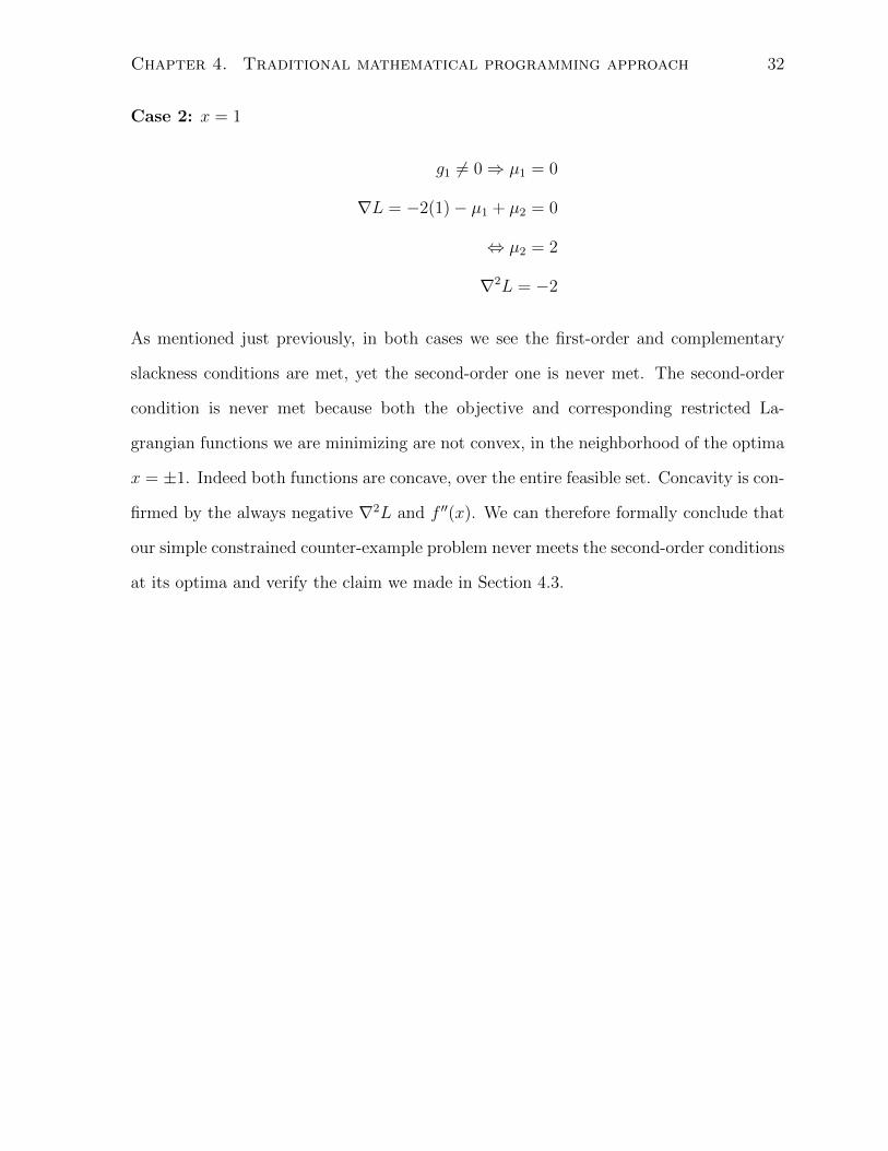
Chapter 4. Traditional mathematical programming approach 32
Case 2: x = 1
g1 6= 0⇒ µ1 = 0
∇L = −2(1)− µ1 + µ2 = 0
⇔ µ2 = 2
∇2L = −2
As mentioned just previously, in both cases we see the first-order and complementary
slackness conditions are met, yet the second-order one is never met. The second-order
condition is never met because both the objective and corresponding restricted La-
grangian functions we are minimizing are not convex, in the neighborhood of the optima
x = ±1. Indeed both functions are concave, over the entire feasible set. Concavity is con-
firmed by the always negative ∇2L and f ′′(x). We can therefore formally conclude that
our simple constrained counter-example problem never meets the second-order conditions
at its optima and verify the claim we made in Section 4.3.

Chapter 5
Properties of the fractionation
problem
In this chapter, we briefly revisit the analytic solutions, from the literature, for the case of
a fractionation problem with a single sensitive structure constraint. We also attempt to
formally characterize all optimum-candidate points, for more general formulations, with
an arbitrary number of sensitive structure constraints. While the most recent literature
only deals with problems constrained by a single sensitive structure, we seek more general
results that can be applied to cases where the treatment dose is constrained by more than
one sensitive structure, as is typically the case in practice.
5.1 Known analytic optima
In the literature, some authors (Keller and Davison, 2008; Mizuta et al., 2012) present
analytic closed-form solutions to the fractionation problem, in the case of a single sensitive
structure constraint. These solutions are based on the relative magnitude of the ratios
33

Chapter 5. Properties of the fractionation problem 34
of the α and β radiosensitivity parameters of the objective and constraint functions.
Here, we review these results and add a minor modification to the theorem of Keller and
Davison (2008), for the cases of equality of ratios. We also explore a specific property of
the optima of the fractionation problem, the boundary property, which we present as a
lemma.
Both Keller and Davison (2008); Mizuta et al. (2012) show that the optimum is either a
large single dose treatment or a dose equally divided into the specified number of dose
fractions that make up the treatment (EQDF). The actual doses can then be determined
by solving the second-degree polynomial formed by the (single) sensitive-tissue constraint.
Recall the fractionation problem with a single sensitive-structure constraint presented in
Chapter 3. The goal is to maximize the tumor cell kill, while keeping the damage to the
sensitive-structure to a preset level.
According to Keller and Davison (2008); Mizuta et al. (2012), if the ratio of the sensitive-
structure’s radiosensitivity parameters (α/ωβ)S is less than the ratio of tumor’s radiosen-
sitivity parameters (α/β)T , then the optimal treatment is an equal-dose-per-fraction
schedule over the entire length of the treatment of N fractions. Otherwise, if the ratio
(α/ωβ)S is greater than the ratio (α/β)T , then the optimal treatment is a dose delivered
in a single fraction. In both cases, the doses (equal-dose-per-fraction or single-dose) are
found by solving the quadratic equations (with one unknown), given by the sensitive-
tissue constraint. Indeed, given that the treatment is either a single dose or N equal
doses, the sensitive-tissue equality constraint becomes a second-degree polynomial in one
variable.
To illustrate this idea, we graphically show how the relative magnitudes of the α/β ratios
affect the shapes and intersections of linear quadratic functions, in a two-fraction (R2)
case. By taking a look at examples in R2, we see that the curvature of the objective
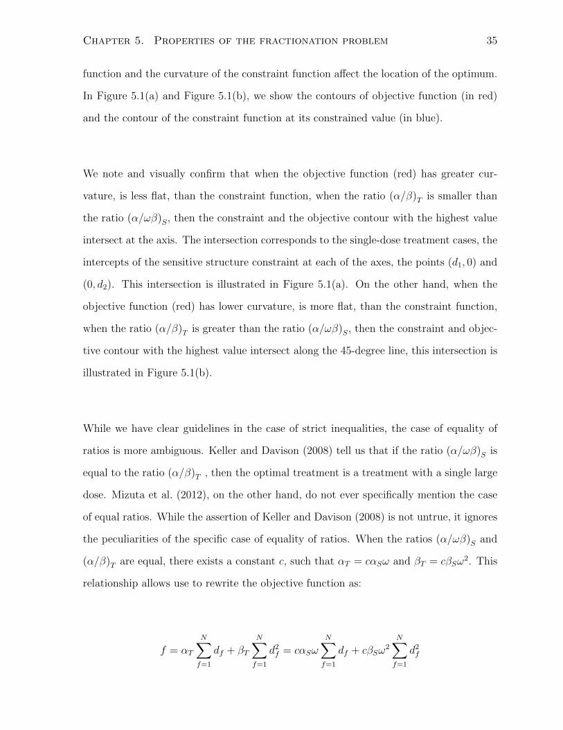
Chapter 5. Properties of the fractionation problem 35
function and the curvature of the constraint function affect the location of the optimum.
In Figure 5.1(a) and Figure 5.1(b), we show the contours of objective function (in red)
and the contour of the constraint function at its constrained value (in blue).
We note and visually confirm that when the objective function (red) has greater cur-
vature, is less flat, than the constraint function, when the ratio (α/β)T is smaller than
the ratio (α/ωβ)S, then the constraint and the objective contour with the highest value
intersect at the axis. The intersection corresponds to the single-dose treatment cases, the
intercepts of the sensitive structure constraint at each of the axes, the points (d1, 0) and
(0, d2). This intersection is illustrated in Figure 5.1(a). On the other hand, when the
objective function (red) has lower curvature, is more flat, than the constraint function,
when the ratio (α/β)T is greater than the ratio (α/ωβ)S, then the constraint and objec-
tive contour with the highest value intersect along the 45-degree line, this intersection is
illustrated in Figure 5.1(b).
While we have clear guidelines in the case of strict inequalities, the case of equality of
ratios is more ambiguous. Keller and Davison (2008) tell us that if the ratio (α/ωβ)S is
equal to the ratio (α/β)T , then the optimal treatment is a treatment with a single large
dose. Mizuta et al. (2012), on the other hand, do not ever specifically mention the case
of equal ratios. While the assertion of Keller and Davison (2008) is not untrue, it ignores
the peculiarities of the specific case of equality of ratios. When the ratios (α/ωβ)S and
(α/β)T are equal, there exists a constant c, such that αT = cαSω and βT = cβSω2. This
relationship allows use to rewrite the objective function as:
f = αT
N∑f=1
df + βT
N∑f=1
d2f = cαSω
N∑f=1
df + cβSω2
N∑f=1
d2f

Chapter 5. Properties of the fractionation problem 36
(a) Contours of the objective (red) and
constraint function (blue), single dose
case
(b) Contours of the objective (red), con-
straint function (blue) and 45 degree line
(black dots), EQDF case
Figure 5.1: Two possible optimal solutions in the single sensitive structure constraint
case, (a) the single dose treatment and (b) the equal dose per fraction treatment

Chapter 5. Properties of the fractionation problem 37
The optimization problem then becomes
maximize c
(αSω
F∑f=1
df + βSω2
F∑f=1
d2f
)
subject to
αSωF∑f=1
df + βSω2
F∑f=1
d2f = K
df ≥ 0 ∀f = 1, . . . , F
This case is degenerate and probably only occurs very rarely. In this case, all feasible
(positive) doses that make the constraint equal K yield exactly the same objective func-
tion value. Therefore, all feasible points are optima, not just the single-dose point, as
claimed in Keller and Davison (2008).
5.2 Change of coordinates
To extract the main mathematical properties of the linear-quadratic function more easily
we change the coordinate system used to represent the dose-per-fraction, from a standard
Rn coordinate system, where each coordinate represents a fractional dose to a more
compact equivalent, described here.
Previously, we expressed the doses for each fraction in a treatment with N fractions as
coordinates of a vector in RN . We called this vector ~d = [d1, . . . , dN ], where di is the
dose delivered to the tumor under treatment, in fraction i.
Any vector in RN can be expressed as a linear combination of a vector of ones ~1N =
[1 . . . 1]T ∈ RN and a vector ~vN ∈ RN that is orthogonal to it and which we have scaled
by its `2-norm, so it has unit length. Therefore, any arbitrary vector ~x ∈ RN can be
expressed as the linear combination ~x = ρ~1N+ε~vN , with the appropriate scalar coefficients

Chapter 5. Properties of the fractionation problem 38
ρ, ε ∈ R.
In this coordinate system, we can identify any point in RN , with only three parameters:
the scalars ρ, ε and the vector ~vN . For example, in R3
[3 4 5] = ρ[1 1 1] + ε[v1 v2 v3]
= 4[1 1 1] + ε
[−1√
20
1√2
]= [4 4 4] +
√2
[−1√
20
1√2
]
Note that the vector ~v3 = [v1 v2 v3] = [−1/√
2 0 1/√
2] is orthogonal to the vector of
ones ~13 = [1 1 1] and is normalized (i.e., scaled by its `2-norm). Its sum of coordinates
is equal to zero and its `2-norm (and sum of squared coordinates) is equal to one, by
design.
In Figure 5.2, we illustrate graphically an example of this change of coordinates, with a
simple example in R2, where we have replaced the traditional unit vectors [1 0] and [0 1]
with the vector [1 1] and an orthogonal vector [ 1√2−1√
2].
Using this new coordinate system, we will express the LQ function for a treatment over
N fractions, where df denotes the dose administered in fraction f . In its original form,
the LQ function was given by
f = α
N∑f=1
df + β
N∑f=1
d2f
Using our new coordinate system, we can re-write our dose-per-fraction vector ~d as
~d = [d1, . . . , dN ]
~d = ρ~1N + ε~vN

Chapter 5. Properties of the fractionation problem 39
[x y]
ρ[1 1]
ε[1/√2 -‐1/√2]
Figure 5.2: Change of coordinates example in R2
The LQ function is re-written as
f = αN∑f=1
df + βN∑f=1
d2f (5.1)
= αN∑i=1
(ρ+ εvi) + βN∑i=1
(ρ+ εvi)2 (5.2)
= α
(N∑i=1
ρ+ εN∑i=1
vi
)+ β
N∑i=1
(ρ2 + 2ρεvi + ε2v2
i
)(5.3)
= α
(N∑i=1
ρ+ ε
N∑i=1
vi
)+ β
(N∑i=1
ρ2 + 2ρεN∑i=1
vi + ε2N∑i=1
v2i
)(5.4)
= α(Nρ+ ε× 0) + β(Nρ2 + 2ρε× 0 + ε2 × 1) (5.5)
= α(Nρ) + β(Nρ2 + ε2) (5.6)
Recall that by construction∑N
i=1 vi = 0,∑N
i=1 v2i = 1, which explains the transition from
equation 5.4 to equation 5.5
While this coordinate system transformation is very helpful in establishing mathematical
properties, as will be seen in the next section, it is of limited value in practice. Indeed,
not all points in RN can be expressed using the same orthogonal vector ~v. If we go back
Chapter 5. Properties of the fractionation problem 40
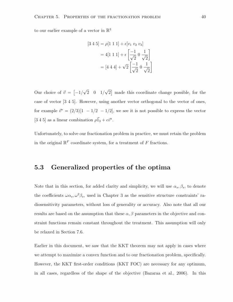
to our earlier example of a vector in R3
[3 4 5] = ρ[1 1 1] + ε[v1 v2 v3]
= 4[1 1 1] + ε
[−1√
20
1√2
]= [4 4 4] +
√2
[−1√
20
1√2
]
Our choice of ~v =[−1/√
2 0 1/√
2]
made this coordinate change possible, for the
case of vector [3 4 5]. However, using another vector orthogonal to the vector of ones,
for example ~v∗ = (2/3)[1 − 1/2 − 1/2], we see it is not possible to express the vector
[3 4 5] as a linear combination ρ~13 + ε~v∗.
Unfortunately, to solve our fractionation problem in practice, we must retain the problem
in the original RF coordinate system, for a treatment of F fractions.
5.3 Generalized properties of the optima
Note that in this section, for added clarity and simplicity, we will use αs, βs, to denote
the coefficients ωαs, ω2βs, used in Chapter 3 as the sensitive structure constraints’ ra-
diosensitivity parameters, without loss of generality or accuracy. Also note that all our
results are based on the assumption that these α, β parameters in the objective and con-
straint functions remain constant throughout the treatment. This assumption will only
be relaxed in Section 7.6.
Earlier in this document, we saw that the KKT theorem may not apply in cases where
we attempt to maximize a convex function and to our fractionation problem, specifically.
However, the KKT first-order conditions (KKT FOC) are necessary for any optimum,
in all cases, regardless of the shape of the objective (Bazaraa et al., 2006). In this
Chapter 5. Properties of the fractionation problem 41
section, we exploit the KKT FOC to formally characterize the optima and extract their
properties, in the case of a problem constrained by an arbitrary number of sensitive
structure constraints.
In the case of a problem constrained by a single sensitive structure, Keller and Davison
(2008); Mizuta et al. (2012) provide an analytic solution for the optima of the fraction-
ation problem. The case of an arbitrary number of sensitive structure constraints, was
not addressed. In this section, we attempt to formally characterize some properties of
the optima, in the more general cases of a problem constrained by an arbitrary number
of sensitive structure constraints. We also attempt to provide a different mathematical
perspective on the results of Keller and Davison (2008); Mizuta et al. (2012) through the
use of the KKT FOC.
We will now prove the fact that the optima are known to always lie on the most restrictive
constraint(s), the constraint(s) that impose the largest restriction on the dose that can
be delivered to the tumor. This property applies not just to problems constrained by a
single sensitive-structure constraint, where it is entirely consistent with the formulations
and results presented in Keller and Davison (2008); Mizuta et al. (2012), but also to more
general problems constrained by an arbitrary number of sensitive-structure constraints.
Lemma 1. The optima for a fractionation problem with a linear-quadratic objective func-
tion with positive radiosenstivity parameters, constrained by one or more linear-quadratic
constraint functions, must lie on the most restrictive sensitive-structure constraint(s). In
other words, at the optimum at least one sensitive-structure constraint must be active.
Proof. (by contradiction)
Let ~̃d = [d̃1, . . . , d̃N ] be a maximum that lies in the interior of the feasible set. That
Chapter 5. Properties of the fractionation problem 42
means that for the given set of constraints gj(~d) ≤ Kj, ∀j = 1, . . . , J we have
gj( ~̃d) =N∑f=1
(αj d̃f + βj d̃2f ) < Kj ∀j = 1, . . . , J
We can replace the first dose d̃1 with a larger dose d∗1 > d̃1, such that for the most
restrictive constraint, call it gr, we get:
gr( ~̃d, d∗1) = (αrd
∗1 + βrd
∗21 ) +
N∑i=2
(αrd̃i + βrd̃2i ) = Kr > gr( ~̃d)
If we go back to the objective, given the parameters α, β and the variables d∗i , d̃i are
always positive, it is clear that the function is monotonically increasing:
(αtd∗1 + βtd
∗21 ) +
N∑i=2
(αtd̃i + βtd̃2i ) >
N∑i=1
(αtd̃i + βtd̃2i )
This inequality contradicts our initial claim that interior point ~̃d was an optimum. There-
fore, the optimum must be on the boundary of the most restrictive sensitive-structure
constraint.
As shown in the single sensitive structure case in Section 5.1, optima occur either the
EQDF point, the intersection of the sensitive tissue constraint with the non-negativity
constraints (which occurs at the the single-dose points), or any positive point along the
boundary of the sensitive-structure constraint. The actual location of the optima de-
pends on the relative magnitude of the radiosensitivity parameters of the objective and
constraint LQ functions, as described by Keller and Davison (2008); Mizuta et al. (2012).
In the case of more than one sensitive structure, these points remain candidates for an
optimum, but additionally (only) the intersections of two or more sensitive structure con-
straints may also be candidates for optima, as we will demonstrate later in this chapter.
Chapter 5. Properties of the fractionation problem 43
In Section 4.1, we have explained why the KKT theorem, its sufficient condition specifi-
cally does not apply to our specific problem. However, the first-order conditions (FOC)
are always necessary for the existence of an optimum. We now examine these conditions,
in the context of the new coordinate system described above, to formally describe some
properties of the optima.
Recall our N -fraction fractionation problem, expressed using the new coordinate system:
minimizeρ,ε f(ρ, ε) = −αt(Nρ)− βt(Nρ2 + ε2)
subject to
gj(ρ, t) = αj(Nρ) + βj(Nρ2 + ε2)−Kj ≤ 0 ∀j = 1, . . . , S
hi(ρ, t) = −ρ− εγi ≤ 0 ∀i = 1, . . . , N
The sensitive tissue constraints for each of the j = 1, . . . , S sensitive-structures are de-
noted by gj and the dose non-negativity constraints for each of the i = 1, . . . , N fractions
are denoted by hi. Also, we use ‘I’ to denote the set of all active constraints.
Theorem 1. The optimum for a fractionation problem with a linear-quadratic objective
function and sensitive structure constraint function of fractional doses occurs in one of
three cases:
(i) at the equal dose per fraction point given by the most restrictive sensitive structure
constraint
(ii) at the intersection of at least two active constraints
(iii) at any feasible boundary point along the most restrictive constraint, in the degenerate
case where the objective and the most restrictive sensitive structure constraint are
multiples of each other.
Proof. Before proving this claim, we note that this problem needs at least one sensitive-

Chapter 5. Properties of the fractionation problem 44
tissue constraint, otherwise it is unbounded and the doses can be infinitely high. Addi-
tionally, because the problem is defined for a non-empty closed bounded feasible set, over
which the objective function is defined and continuous, an optimum exists. Finally, as
shown in lemma 1, at least one sensitive tissue constraint will be tight, at the optimum.
We also need to recall that we only deal with feasible positive doses, as feasibility must
always be met, at any optimum.
Recall that for our fractionation problem, at an optimum, the following must hold (by
KKT FOC and feasibility conditions).
∇L = ∇f +∑j∈I
(µj∇gj) +∑i∈I
(µi∇hi) = ~0
gj, hi ≤ 0 ∀i, j ∈ I
µj, µi ≥ 0 ∀i, j ∈ I
µj, µi = 0, if gj, hi < 0 ∀i, j /∈ I
Here the functions gj denote the sensitive structure constraints, the functions hi the dose
non-negativity constraints and I the set of all active constraints.
Now, let the optimum occur at a point where only one sensitive-structure constraint,
namely gj∗ , is active and all other gj, hi < 0, in other words none of the doses di > 0
violate any constraint.
At such an optimum, the KKT FOC gives us the following equality. (Recall that all but
one µ = 0, namely µj∗ ≥ 0.)
∇L = ∇f + µj∗∇gj∗ = ~0
From the KKT FOC. we get two possible cases µj∗ = 0 or µj∗ > 0

Chapter 5. Properties of the fractionation problem 45
Case 1: µj∗ = 0 (i.e., ∇f = 0)
∇L =
−αtN − 2βtNρ
−2βtε
=
0
0
Recall that αt, n, βt, λ > 0, so this equality can never hold, since the inequality −αtn 6=
2βtnλ is always true. Therefore, we can conclude Case 1 will never occur.
Case 2: µj∗ > 0
∇L =
−αtN − 2βtNρ+ µj∗(αj∗N + 2βj∗Nρ)
−2βtε+ 2µj∗βj∗ε
=
0
0
This equality means that βtε = µj∗βj∗r or, in the case of an arbitrary ε 6= 0, that
βt = µj∗βj∗ . From Case 2, we see only two possibilities:
A) If ε = 0 (i.e., only candidate for an optimum is the EQDF point given by the j∗th
constraint)
(a) αt + 2βtρ = µj∗αj∗ + 2µj∗βj∗ρ, for some µj∗ , ρ pair
(b) βtε = µj∗βj∗ε, which is always true (i.e., 0 = 0)
B) If ε 6= 0 (i.e., The only candidate for an optimum is not the EQDF point)
(a) αt + 2βtρ = µj∗αj∗ + 2µj∗βj∗ρ = µj∗(αj∗ + 2βj∗ρ)
(b) βtε = µj∗βj∗ε⇔ βt = µj∗βj∗
In the case where ε 6= 0, when the EQDF point is not the sole candidate for an optimum,
we see that αt + 2µj∗βj∗ρ = µj∗αj∗ + 2µj∗βj∗ρ ⇒ αt = µj∗αj∗ and of course βt =
Chapter 5. Properties of the fractionation problem 46
µj∗βj∗ . The constraint is a multiple of the objective, so all (positive dose) points on the
boundary satisfy the FOC, yield the same objective function value and are candidates
for an optimum.
The only possible candidates for an optimum, when only one sensitive structure con-
straint is tight, are the points where ε = 0, which are equal-dose-per-fraction points, or
all arbitrary points on the boundary, in the (degenerate) case where the objective and
constraint function are multiples of each other. This proves the assertions in case (i) and
in case (iii) of the theorem statement.
For any other point to be a candidate for an optimum we need to introduce more active
constraints, which will intersect, by definition. These intersections, then become the
only feasible points and are therefore the only possible candidates for an optimum. For
example, if two constraints were active, at the optimum, we would get the equality:
∇L = ∇f + µj∗∇gj∗ + µj̃∇gj̃ = ~0
In this scenario the optimum can only occur at the intersection of the active constraints
gj∗ and gj̃, by definition, since both are active. This proves the assertion in case (ii) of
the theorem statement.
In summary, it has been shown that with only one active sensitive-tissue constraint
a boundary equal-dose-per-fraction treatment or any arbitrary point on the boundary
are the only possible candidates for optima. Any other specific optimum candidate
point would require at least one more active constraint. Therefore we can claim that an
optimum, in the case where more than one constraint is active, must occur an intersection
of these constraints, by definition.
In the work of Keller and Davison (2008) and Mizuta et al. (2012), which deal with the
special case of a single sensitive structure constraint, the optima are shown to occur only

Chapter 5. Properties of the fractionation problem 47
in the equal-dose-per-fraction case or in the single-dose case. The equal-dose-per-fraction
optimum corresponds to a situation where ε = 0 and is shown here in Case 2. The single-
dose optimum corresponds to the intersection of multiple constraints, the sensitive tissue
constraint and all but one of the non-negativity constraints. Our conclusions are therefore
entirely consistent with the conclusions reached by these authors.
In the case of multiple sensitive tissue constraints, the intersection of these constraints
offer an additional set of potential candidates for optima. Future work may involve
solving the system of constraints to find all constraint intersection points and evaluate
the objective at each of these points, in order to solve this problem exactly.
Chapter 6
Simulated annealing
We have shown that the fractionation problem cannot be solved using conventional math-
ematical programming techniques and that we must resort to a numerical search global
optimization technique, to obtain our solution. Unfortunately, these techniques are com-
putationally costly and typically do not guarantee optimality of the solution. In our
case, it is important for the reader to understand that we are not looking for a provable
global optimum. Our goals are a lot more modest. Currently, clinical practice conven-
tion splits up the total prescribed dose into equal doses in each fraction. Our goal is
to verify whether or not a different fractionation scheme may yield better results within
the framework imposed by the linear-quadratic model, described in Fowler (1992); Bren-
ner et al. (1998); Brenner (2008); Kirkpatrick et al. (2008) or, in the alternate case, to
validate current conventional practices. We look for improved treatment plans that do
not differ drastically from current clinical norms and from the solutions proposed in the
literature, which guides our numerical search and allows us to validate our results. We
use the known optima in the single-dose and “equal-dose-per-fraction” cases to test our
computational technique and to empirically validate the theorem presented in Keller and
Davison (2008); Mizuta et al. (2012), for the case of a single sensitive-structure constraint,
48

Chapter 6. Simulated annealing 49
where we have the benefit of existing analytical solutions.
In Keller and Davison (2008) the authors solve the fractionation using dynamic pro-
gramming. We investigated three alternate solution techniques: the application of the
KKT theorem, non-linear projected gradient, and an array of global optimization search
algorithms. In the end, we settled on simulated annealing as our numerical optimization
technique of choice. A thorough comparison of heuristic techniques is beyond the scope
of this document, but we justify our final choice of simulated annealing on the basis that
it is widely accepted and used in the medical physics literature in general, for example
Webb (1989); Morrill et al. (1991); Mageras and Mohan (1993); Aleman et al. (2008); Cao
et al. (2012), and notably in a different formulation of the dose fractionation problems
(Yang and Xing, 2005), on the fact that it is known simulated annealing yields a global
optimum, given a long enough cooling period (Brownlee, 2011) and on the basis of the
“no free lunch theorem” (Wolpert and Macready, 1997; Brownlee, 2011).
To account for the sensitive structure constraints, we transformed our (continuous con-
strained) problem into a continuous unconstrained one, by substituting a penalized ob-
jective function for the original objective. Our penalty formulation was also designed to
accommodate an arbitrary number of sensitive-structure constraints.
We faced a number of options with this technique and we did a bit of tailoring to the
common simulated annealing technique before applying it to the particulars of the frac-
tionation problem. Following the recommendation in Wah and Wang (1999), we relaxed
our problem stated in Chapter 3 by converting our equality constraint, in the single
sensitive structure case, into an inequality constraint (≤), which was integrated into the
penalized objective function discussed in Chapter 6. This relaxation later allowed us to
overcome possible inconsistencies in the constraints (and an empty feasible set), in the
case of multiple constraints. Also, according to Wah and Wang (1999) this relaxation
enhances the search and increases the likelihood of attaining a global optimum.
Chapter 6. Simulated annealing 50
We also devised two distinct search strategies to explore the feasible set. In one case,
we explore only the boundary of the feasible set, where the optimum is known to lie (as
shown in Section 5.3) and in another case, we explore the interior of the feasible set, as
well as its boundary. Although we know the optima must lie on the boundary comparing
these two search strategies provides further validation of our numerical technique.
The penalized functions fp we seek to maximize through simulated annealing, in each of
the two cases, is given by
f rp (~d) = f(~d)− P ×max[0, (gj(~d)−K)] (regular simulated annealing algorithm) (6.1)
f bp(~d) = f(~d)− P × [0, (gj(~d)−K)]2 (boundary algorithm) (6.2)
where f(~d) is the objective (radiation effect) function we are maximizing, gj(~d) the j− th
healthy structure constraint function and K is the right hand side of the constraint
gj(~d) ≤ K. In the first case (regular algorithm), infeasible solutions, solutions for which
gj(~d) − K > 0 are penalized by a large penalty coefficient P (� 0). In the second
case (boundary algorithm), all solutions not lying on the boundary are penalized by a
coefficient P (which is why we take the square of all deviations from the boundary) .
This algorithm steers the search of the feasible set toward the boundary. Naturally, we
also exclude from our search any dose vector ~d with negative coordinates, by rejecting
any move to a point with negative coordinates.
In the case of more than one sensitive-structure constraint, we pick the largest devia-
tion, since we are looking to minimize deviation from the boundary formed by the most
restrictive set of constraints:
f rp (~d) = f(~d)− P ×maxj{max[0, (gj(~d)−Kj)]} (6.3)
f bp(~d) = f(~d)− P ×max
j{max[(gj(~d)−Kj)]
2} (6.4)
Where f rp in equation 6.3 is the regular search penalized objective function and f bp in
equation 6.4 is the boundary search penalized objective function. The mechanics of this

Chapter 6. Simulated annealing 51
g(x)−K<0
g(x)−K>0
g(x)−K=0
Figure 6.1: Penalty scheme on interior and exterior of the feasible set
penalty scheme are illustrated in Figure 6.1. The steps of the simulated algorithm are
described in Algorithm 1, with the five following user-specified variables:
1. S0: starting point
2. T0: starting temperature
3. Ck: cooling constant
4. I: total number of iterations (stopping criterion)
5. r: search radius
and the randomly generated (U(-1,1)) step direction vector, denoted by ~s. The new point
is the current point plus some random step direction, multiplied by a fixed radius r. This
random uniform step allows the exploration of increasing and decreasing coordinates
(fraction doses).
In the following chapter, we will assess the quality of the solutions yielded by our sim-

Chapter 6. Simulated annealing 52
Algorithm 1 Function maximization via simulated annealing (Brownlee, 2011)
1: i← 0
2: T ← T0
3: x̄← S0
4: x(i) ← x̄
5: best ← x(i)
6: while i ≤ N do
7: i← i+ 1
8: ~s← rand(U(-1,1))
9: x̄← x(i−1) + r × ~s
10: if fp(x̄) ≥ fp(x(i−1) then
11: best ← x̄
12: end if
13: Pr ← exp(
[fp(x̄)−fp(x(i−1))]
T
)14: if Pr ≥ rand(U(0,1)) then
15: x(i) ← x̄
16: else
17: x(i) ← x(i−1)
18: end if
19: T ← temp×Ck
20: end while
21: return best
Chapter 6. Simulated annealing 53
ulated annealing routine variations. We will compare the performance of the boundary
and interior search algorithms and the effect of the different parameters on the final
solution.
In order to efficiently compare solutions obtained by our simulated annealing routine,
in each of our trials we sort the solution doses, in descending order. According to this
convention, larger doses are delivered first. This re-arrangement is in line with the spirit
of Keller and Davison (2008), who apply this convention to their results as well. Also, this
re-arrangement does not affect the value of the linear-quadratic functions, as discussed
in Section 2.1. Re-arranging doses in this way allows for a clearer comparison of results
yielded by the different variations of our algorithm. Indeed, two treatments may have
the same tumor/sensitive-structure cell kill/cell survival characteristics but have different
ordering of the doses, since the doses in the linear-quadratic model do not have time-
dependency. A large dose followed by a small dose have the same effect as a small
dose followed by a large dose, when the doses are equal to each other, as described in
Chapter 3.
Finally, we classify a solution as being an equal dose per fraction, when the solution
returned by the simulated annealing has approximately equal doses in each fraction,
when the dose are all within a band of ±50% maximum to minimum ratio. When this
ratio is of an the order of two or more, then we classify our solution as a single dose
treatment and we round up the largest dose to the nearest integer and set all others
fractional dose to zero, while ensuring the treatment is still feasible.

Chapter 7
Numerical results
Two rounds of tests were conducted. The first round was aimed at tuning the parameters
of the simulated annealing algorithm. The second round was conducted once the most
suitable simulated annealing parameters had been found, to assess solution quality, for
hypothetical patient cases.
In all our tests, we compared the results obtained by our simulated annealing algorithm,
which we denote as z̄, against the solutions taken from the conclusions of Keller and
Davison (2008); Mizuta et al. (2012), in cases where the problem involved only a single
sensitive-structure constraint, these authors provided us with analytic solutions. Where
the problem involved more than one single sensitive-structure constraint, we compared
our numerical results against the highest feasible single dose treatment and the highest
feasible equal dose treatment, which can be found by solving for the roots of of the linear-
quadratic constraints. Indeed, when it is known the solution is either an equal dose or
single treatment, the sensitive structure constraint becomes a polynomial in only one
unknown variable.
54
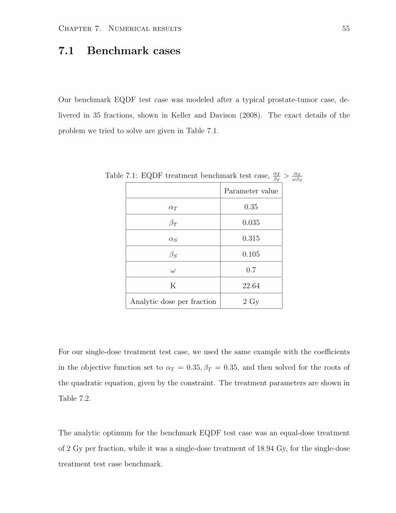
Chapter 7. Numerical results 55
7.1 Benchmark cases
Our benchmark EQDF test case was modeled after a typical prostate-tumor case, de-
livered in 35 fractions, shown in Keller and Davison (2008). The exact details of the
problem we tried to solve are given in Table 7.1.
Table 7.1: EQDF treatment benchmark test case, αT
βT> αS
ωβS
Parameter value
αT 0.35
βT 0.035
αS 0.315
βS 0.105
ω 0.7
K 22.64
Analytic dose per fraction 2 Gy
For our single-dose treatment test case, we used the same example with the coefficients
in the objective function set to αT = 0.35, βT = 0.35, and then solved for the roots of
the quadratic equation, given by the constraint. The treatment parameters are shown in
Table 7.2.
The analytic optimum for the benchmark EQDF test case was an equal-dose treatment
of 2 Gy per fraction, while it was a single-dose treatment of 18.94 Gy, for the single-dose
treatment test case benchmark.
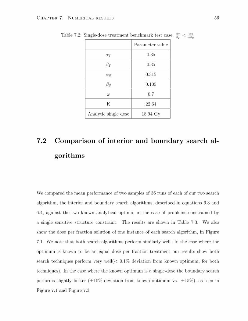
Chapter 7. Numerical results 56
Table 7.2: Single-dose treatment benchmark test case, αT
βT< αS
ωβS
Parameter value
αT 0.35
βT 0.35
αS 0.315
βS 0.105
ω 0.7
K 22.64
Analytic single dose 18.94 Gy
7.2 Comparison of interior and boundary search al-
gorithms
We compared the mean performance of two samples of 36 runs of each of our two search
algorithm, the interior and boundary search algorithms, described in equations 6.3 and
6.4, against the two known analytical optima, in the case of problems constrained by
a single sensitive structure constraint. The results are shown in Table 7.3. We also
show the dose per fraction solution of one instance of each search algorithm, in Figure
7.1. We note that both search algorithms perform similarly well. In the case where the
optimum is known to be an equal dose per fraction treatment our results show both
search techniques perform very well(< 0.1% deviation from known optimum, for both
techniques). In the case where the known optimum is a single-dose the boundary search
performs slightly better (±10% deviation from known optimum vs. ±15%), as seen in
Figure 7.1 and Figure 7.3.
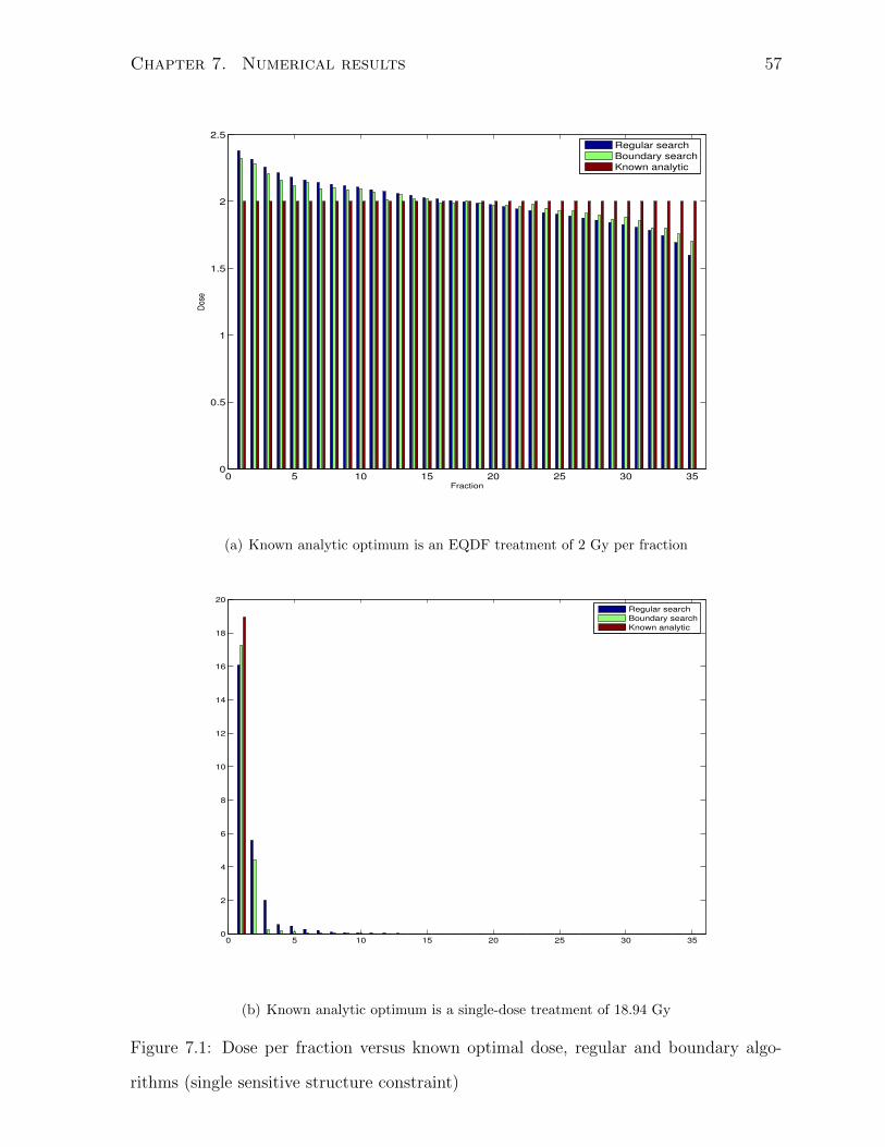
Chapter 7. Numerical results 57
0 5 10 15 20 25 30 350
0.5
1
1.5
2
2.5
Fraction
Dos
e
Regular search
Boundary search
Known analytic
(a) Known analytic optimum is an EQDF treatment of 2 Gy per fraction
0 5 10 15 20 25 30 350
2
4
6
8
10
12
14
16
18
20
Regular search
Boundary search
Known analytic
(b) Known analytic optimum is a single-dose treatment of 18.94 Gy
Figure 7.1: Dose per fraction versus known optimal dose, regular and boundary algo-
rithms (single sensitive structure constraint)
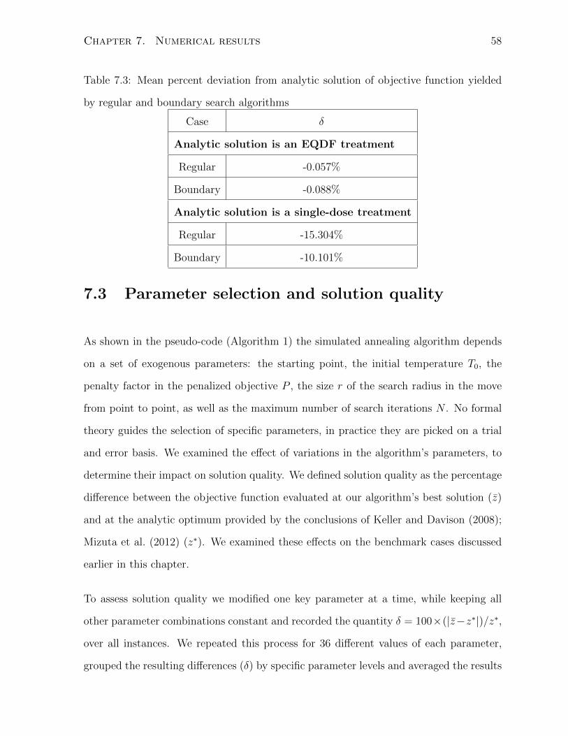
Chapter 7. Numerical results 58
Table 7.3: Mean percent deviation from analytic solution of objective function yielded
by regular and boundary search algorithms
Case δ
Analytic solution is an EQDF treatment
Regular -0.057%
Boundary -0.088%
Analytic solution is a single-dose treatment
Regular -15.304%
Boundary -10.101%
7.3 Parameter selection and solution quality
As shown in the pseudo-code (Algorithm 1) the simulated annealing algorithm depends
on a set of exogenous parameters: the starting point, the initial temperature T0, the
penalty factor in the penalized objective P , the size r of the search radius in the move
from point to point, as well as the maximum number of search iterations N . No formal
theory guides the selection of specific parameters, in practice they are picked on a trial
and error basis. We examined the effect of variations in the algorithm’s parameters, to
determine their impact on solution quality. We defined solution quality as the percentage
difference between the objective function evaluated at our algorithm’s best solution (z̄)
and at the analytic optimum provided by the conclusions of Keller and Davison (2008);
Mizuta et al. (2012) (z∗). We examined these effects on the benchmark cases discussed
earlier in this chapter.
To assess solution quality we modified one key parameter at a time, while keeping all
other parameter combinations constant and recorded the quantity δ = 100×(|z̄−z∗|)/z∗,
over all instances. We repeated this process for 36 different values of each parameter,
grouped the resulting differences (δ) by specific parameter levels and averaged the results

Chapter 7. Numerical results 59
for each parameter level. For all tests, with the exception of the test for starting points, we
seeded Matlab’s random number generator, before each run of the algorithm, to remove
any possible effect from the state of the random number generation routine. The results
are reported in the Figures 7.2(a) to 7.5(b).
10 50 100
0.2
0.4
0.6
0.8
1
1.2
1.4
T0
δ (%
)
(a) Initial temperature v. δ, EQDF case
10 50 1000
1
2
3
4
5
6
7
8
9
T0
δ (%
)
(b) Initial temperature v. δ, single dose treatment case case
Figure 7.2: Effect of initial temperature (T0) on mean percent divergence from known
optimum (δ)
We set the initial temperature to T0 = 100, since it offered a drop-off in the divergence
from the known optimum, in the single dose treatment case, while it had no significant
effect in the EQDF case, as seen in Figure 7.2.

Chapter 7. Numerical results 60
0.25 0.5 10
0.2
0.4
0.6
0.8
1
1.2
1.4
r
δ (%
)
(a) Search radius v. δ, EQDF case
0.25 0.5 10
1
2
3
4
5
6
7
8
r
δ (%
)
(b) Search radius v. δ, single dose treatment case case
Figure 7.3: Effect of search radius (r) on mean percent divergence from known optimum
(δ)
We set the search radius r = 0.25 as it offered the best results for the EQDF case and
results comparable to the best outcome in the single dose treatment case, as shown in
Figure 7.3.
We set our penalty coefficient P = 100, since it offers the best results in the single dose
treatment case, while its variation seems to have virtually no effect on solution accuracy,
in the EQDF case, as seen in Figure 7.4.

Chapter 7. Numerical results 61
100 500 10000
0.2
0.4
0.6
0.8
1
1.2
1.4
P
δ (%
)
(a) Penalty coefficient v. δ, EQDF case
100 500 10000
1
2
3
4
5
6
7
8
9
P
δ (%
)
(b) Penalty coefficient v. δ, single dose treatment case case
Figure 7.4: Effect of penalty coefficient (P ) on mean percent divergence from known
optimum (δ)
The number of iterations (N) is the stopping criterion for the simulated annealing algo-
rithm, once the algorithm has performed N searches it stops and returns its best solution.
We chose a maximum number of iterations N = 500, 000 because it offered an error rate
of ±5% in the singe-dose case and ≤ 1% in the EQDF case, while keeping runtimes
reasonable (±1 minute), as can be seen in Figure 7.5.
Finally, in order to measure the effect of starting points on the quality of the solution
obtained, solutions obtained from starting points that were randomly generated were

Chapter 7. Numerical results 62
10K 100K 500K 5.2M0
0.2
0.4
0.6
0.8
1
1.2
1.4
1.6
1.8
N
δ (%
)
(a) Number of iterations v. δ, EQDF case
10K 100K 500K 5.2M0
2
4
6
8
10
12
14
16
N
δ (%
)
(b) Number of iterations v. δ, single dose treatment case case
Figure 7.5: Effect of number of iterations (N) on mean percent divergence from known
optimum (δ)
compared to ”warm starts” in which the starting point is the end point of a previous
run of the algorithm. We generated a sample of 36 results with a random starting point
and a sample of 36 results with a warm start and then performed a two-sample t-test
to see if we could reject the null hypothesis that the mean objective function value was
statistically different from one sample to the other. We conducted this experiment on
both benchmark cases. Our null hypothesis was that if start point affects the solution,
then the mean objective function values obtained in each sample will be statistically

Chapter 7. Numerical results 63
Table 7.4: Two-sample t-test, null hypothesis of equal means, regardless of starting point
Statistic EQDF case Single dose case
Mean rand start 29.373 111.964
Stdev rand start 0.181 2.874
Mean warm start 29.365 118.859
Stdev warm start 0.142 2.988
t statistic 0.083 -16.848
degrees of freedom 67 68
p value 0.23 0
different and we will not reject it.
Unlike the other tests for parameter sensitivity, we employed statistical significance test-
ing, instead of simple numerical comparison of the effect of parameter variations on the
solution, because our data points were randomly generated and for greater sampling
variety. For a treatment with N fractions, our starting point is a variable in RN , to ad-
equately observe the effect of variations in starting point on solution quality, one would
have to test for increases and decreases in all N dimensions, a combinatorially large task.
Instead, we conducted a comparison of result samples obtained from random and warm
start starting points for an objective and constraint function combination that have a
known analytically-derived optimum was an equal dose per fraction and one where the
known optimum was a single-dose treatment. The results of this test are reported, in
Table 7.4. For the mechanics of the t-test, we followed the procedure outline in Devore
(2000).
We see that in the case of the single-dose treatment the null hypothesis that both means
are indistinguishable is rejected. This rejection of the null hypothesis means the warm
start appears to yield better results (higher objective function value) in the single-dose

Chapter 7. Numerical results 64
case. Therefore all our further runs were done with warm starts. That means we ran our
algorithm once, using a random start, recorded the end point and used that end point
as a starting point for another run. The results of the second run were the one that were
retained. Although the warm start procedure increased runtimes, they remained very
reasonable (less than 2 minutes).
We may conclude that comparing various algorithm parameter settings allowed us to
fine-tune our algorithm to obtain the best possible solutions. Our solutions also seemed
to numerically validate the conclusions presented in Keller and Davison (2008); Mizuta
et al. (2012).
7.4 Single tumor, single sensitive structure case
The first hypothetical patient cases are cases with only one sensitive structure constraint.
In these cases we have the benefit of testing our solutions against the known optima of
Keller and Davison (2008); Mizuta et al. (2012). We compare our solution against the
known analytic optima, in both benchmark test cases, described at the beginning of this
chapter.
In Figure 7.6 and Table 7.5 we see that our simulated annealing is able to virtually
replicate the benchmark case and yields a solution that is only 0.03 % worse than the
known optimum, in the case where the optimum is known to be an EQDF treatment of
2 Gy per fraction. In the case where the optimum is known to be a single dose of 18.94
Gy, our solution yields an objective function value that is roughly 10% worse than the
optimal.
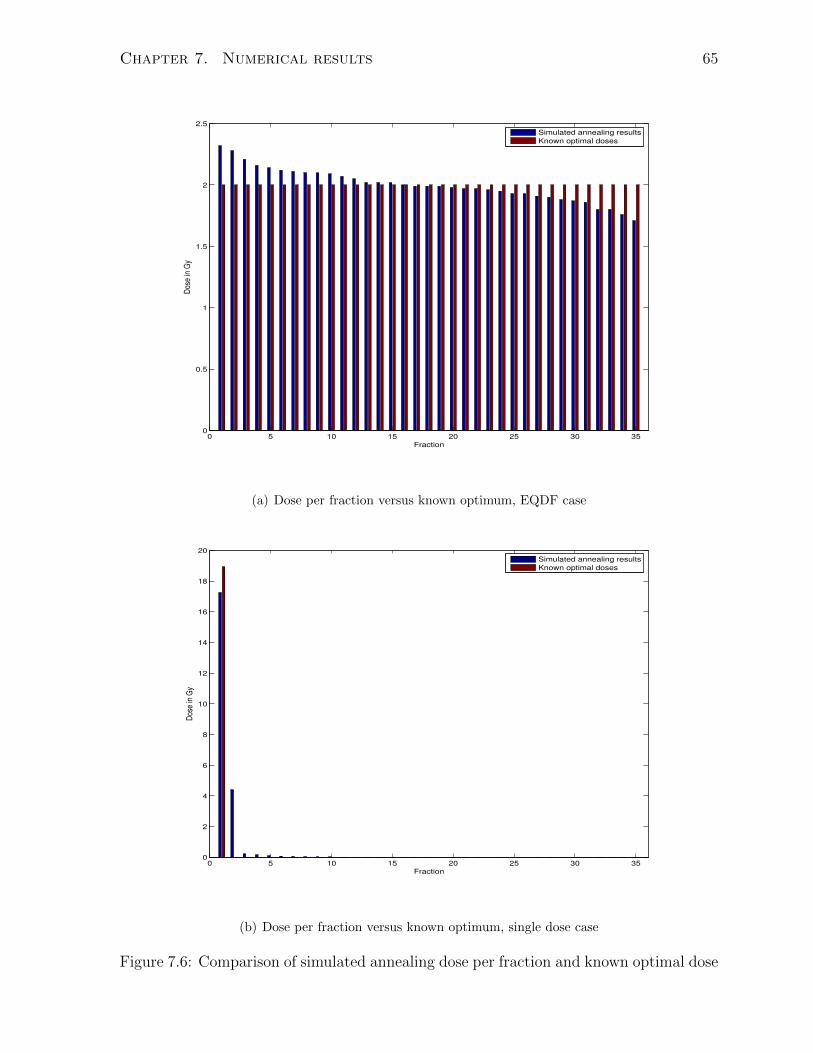
Chapter 7. Numerical results 65
0 5 10 15 20 25 30 350
0.5
1
1.5
2
2.5
Fraction
Dos
e in
Gy
Simulated annealing results
Known optimal doses
(a) Dose per fraction versus known optimum, EQDF case
0 5 10 15 20 25 30 350
2
4
6
8
10
12
14
16
18
20
Fraction
Dos
e in
Gy
Simulated annealing results
Known optimal doses
(b) Dose per fraction versus known optimum, single dose case
Figure 7.6: Comparison of simulated annealing dose per fraction and known optimal dose
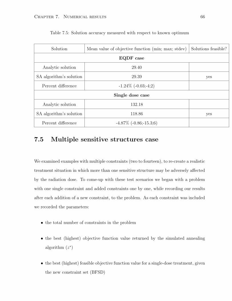
Chapter 7. Numerical results 66
Table 7.5: Solution accuracy measured with respect to known optimum
Solution Mean value of objective function (min; max; stdev) Solutions feasible?
EQDF case
Analytic solution 29.40
SA algorithm’s solution 29.39 yes
Percent difference -1.24% (-0.03;-4;2)
Single dose case
Analytic solution 132.18
SA algorithm’s solution 118.86 yes
Percent difference -4.87% (-0.86;-15.3;6)
7.5 Multiple sensitive structures case
We examined examples with multiple constraints (two to fourteen), to re-create a realistic
treatment situation in which more than one sensitive structure may be adversely affected
by the radiation dose. To come-up with these test scenarios we began with a problem
with one single constraint and added constraints one by one, while recording our results
after each addition of a new constraint, to the problem. As each constraint was included
we recorded the parameters:
• the total number of constraints in the problem
• the best (highest) objective function value returned by the simulated annealing
algorithm (z∗)
• the best (highest) feasible objective function value for a single-dose treatment, given
the new constraint set (BFSD)

Chapter 7. Numerical results 67
• the best (highest) feasible objective function value for a equal-dose treatment, given
the new constraint set (BFEQDF)
• the number of active constraints
• the parameters α, β, ω of the last constraint added to the problem
• the right-hand side value of last constraint added to the problem (Kj)
Unfortunately, in these general cases of multiple sensitive structure constraints, unlike
the case of a single constraint where the analytical optima were given by Keller and
Davison (2008); Mizuta et al. (2012), we do not benefit from a known benchmark for the
optimum. We compare our results to the best feasible single-dose and equal dose per
fraction treatments allowed by our set of constraints, as a “reality check”. Our initial
results suggest, for the examples we encountered, that only the most restrictive constraint
plays a role in the optimum and that the problems we examined can be simplified into
the form of a problem with only one sensitive-tissue constraint, for which results from
Keller and Davison (2008); Mizuta et al. (2012) may be applied.
While the most restrictive constraint may be difficult to identify, prior to running our
simulated annealing algorithm on the entire problem, it is easy to identify it once the
algorithm has been run. The most restrictive constraint(s) will be tight at the conclusion
of the simulated annealing run, since the optimum occurs on the boundary of the feasible
set and this boundary in our problem is defined by the most restrictive constraint(s).
Such a case is shown in Table 7.6, where we see that problem is entirely defined by the
second constraint, which make all 13 other constraints irrelevant.
We recomputed results for this same problem but shuffled the order in which the con-
straints were introduced into the problem. We notice the exact same behavior, except
that the dominant, most restrictive, constraint is now the seventh constraint. We note

Chapter 7. Numerical results 68
Table 7.6: Numerical results, multiple constraint EQDF cases, second constraint domi-
nates. BFSD denotes the value of the objective at the best feasible single-dose solution
given the set of constraints and BFEQDF denotes the value of the objective at the best
feasible equal-dose solution given the same set of constraints
Tot constr z∗ BFSD BFEQDF Active αj βj ωj Kj
1 29.39 19.18 29.40 1 0.32 0.11 0.70 22.64
2 22.59 12.39 22.61 1 0.37 0.18 0.71 22.64
3 22.59 12.39 22.61 1 0.32 0.03 0.65 22.59
4 22.59 12.39 22.61 1 0.38 0.10 0.65 22.64
5 22.59 12.39 22.61 1 0.37 0.17 0.70 22.64
6 22.59 12.39 22.61 1 0.28 0.11 0.71 22.64
7 22.59 12.39 22.61 1 0.36 0.14 0.74 22.70
8 22.59 12.39 22.61 1 0.29 0.05 0.70 22.72
9 22.59 12.39 22.61 1 0.32 0.04 0.75 22.68
10 22.59 12.39 22.61 1 0.39 0.10 0.72 22.61
11 22.59 12.39 22.61 1 0.23 0.04 0.71 22.61
12 22.59 12.39 22.61 1 0.39 0.18 0.65 22.64
13 22.59 12.39 22.61 1 0.34 0.16 0.74 22.58
14 22.59 12.39 22.61 1 0.30 0.05 0.70 22.71
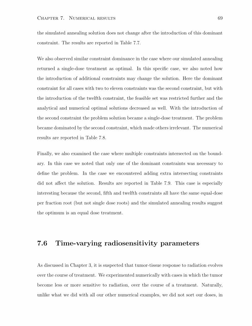
Chapter 7. Numerical results 69
the simulated annealing solution does not change after the introduction of this dominant
constraint. The results are reported in Table 7.7.
We also observed similar constraint dominance in the case where our simulated annealing
returned a single-dose treatment as optimal. In this specific case, we also noted how
the introduction of additional constraints may change the solution. Here the dominant
constraint for all cases with two to eleven constraints was the second constraint, but with
the introduction of the twelfth constraint, the feasible set was restricted further and the
analytical and numerical optimal solutions decreased as well. With the introduction of
the second constraint the problem solution became a single-dose treatment. The problem
became dominated by the second constraint, which made others irrelevant. The numerical
results are reported in Table 7.8.
Finally, we also examined the case where multiple constraints intersected on the bound-
ary. In this case we noted that only one of the dominant constraints was necessary to
define the problem. In the case we encountered adding extra intersecting constraints
did not affect the solution. Results are reported in Table 7.9. This case is especially
interesting because the second, fifth and twelfth constraints all have the same equal-dose
per fraction root (but not single dose roots) and the simulated annealing results suggest
the optimum is an equal dose treatment.
7.6 Time-varying radiosensitivity parameters
As discussed in Chapter 3, it is suspected that tumor-tissue response to radiation evolves
over the course of treatment. We experimented numerically with cases in which the tumor
become less or more sensitive to radiation, over the course of a treatment. Naturally,
unlike what we did with all our other numerical examples, we did not sort our doses, in

Chapter 7. Numerical results 70
Table 7.7: Numerical results, multiple constraint EQDF cases, seventh constraint domi-
nates. BFSD denotes the value of the objective at the best feasible single-dose solution
given the set of constraints and BFEQDF denotes the value of the objective at the best
feasible equal-dose solution given the same set of constraints
Tot constr z∗ BFSD BFEQDF Active αj βj ωj Kj
1 29.39 19.18 29.40 1 0.32 0.11 0.70 22.64
2 23.38 13.78 23.41 1 0.36 0.14 0.74 22.70
3 23.38 13.78 23.41 1 0.32 0.03 0.65 22.59
4 23.38 13.78 23.41 1 0.38 0.10 0.65 22.64
5 23.38 13.78 23.41 1 0.37 0.17 0.70 22.64
6 23.38 13.78 23.41 1 0.28 0.11 0.71 22.64
7 22.59 12.39 22.61 1 0.37 0.18 0.71 22.64
8 22.59 12.39 22.61 1 0.29 0.05 0.70 22.72
9 22.59 12.39 22.61 1 0.32 0.04 0.75 22.68
10 22.59 12.39 22.61 1 0.39 0.10 0.72 22.61
11 22.59 12.39 22.61 1 0.23 0.04 0.71 22.61
12 22.59 12.39 22.61 1 0.39 0.18 0.65 22.64
13 22.59 12.39 22.61 1 0.34 0.16 0.74 22.58
14 22.59 12.39 22.61 1 0.30 0.05 0.70 22,71
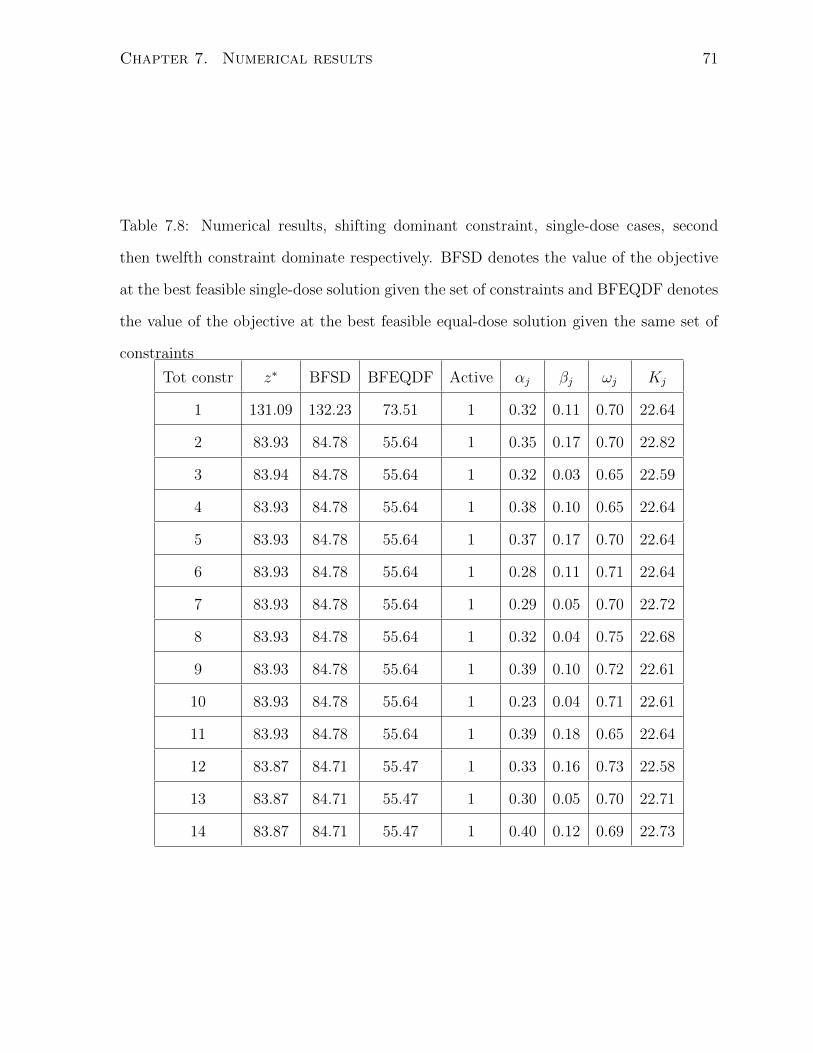
Chapter 7. Numerical results 71
Table 7.8: Numerical results, shifting dominant constraint, single-dose cases, second
then twelfth constraint dominate respectively. BFSD denotes the value of the objective
at the best feasible single-dose solution given the set of constraints and BFEQDF denotes
the value of the objective at the best feasible equal-dose solution given the same set of
constraints
Tot constr z∗ BFSD BFEQDF Active αj βj ωj Kj
1 131.09 132.23 73.51 1 0.32 0.11 0.70 22.64
2 83.93 84.78 55.64 1 0.35 0.17 0.70 22.82
3 83.94 84.78 55.64 1 0.32 0.03 0.65 22.59
4 83.93 84.78 55.64 1 0.38 0.10 0.65 22.64
5 83.93 84.78 55.64 1 0.37 0.17 0.70 22.64
6 83.93 84.78 55.64 1 0.28 0.11 0.71 22.64
7 83.93 84.78 55.64 1 0.29 0.05 0.70 22.72
8 83.93 84.78 55.64 1 0.32 0.04 0.75 22.68
9 83.93 84.78 55.64 1 0.39 0.10 0.72 22.61
10 83.93 84.78 55.64 1 0.23 0.04 0.71 22.61
11 83.93 84.78 55.64 1 0.39 0.18 0.65 22.64
12 83.87 84.71 55.47 1 0.33 0.16 0.73 22.58
13 83.87 84.71 55.47 1 0.30 0.05 0.70 22.71
14 83.87 84.71 55.47 1 0.40 0.12 0.69 22.73
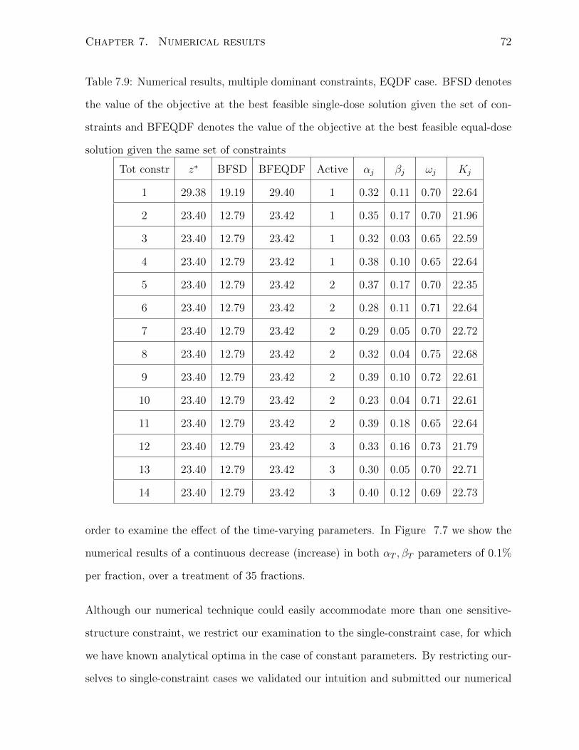
Chapter 7. Numerical results 72
Table 7.9: Numerical results, multiple dominant constraints, EQDF case. BFSD denotes
the value of the objective at the best feasible single-dose solution given the set of con-
straints and BFEQDF denotes the value of the objective at the best feasible equal-dose
solution given the same set of constraints
Tot constr z∗ BFSD BFEQDF Active αj βj ωj Kj
1 29.38 19.19 29.40 1 0.32 0.11 0.70 22.64
2 23.40 12.79 23.42 1 0.35 0.17 0.70 21.96
3 23.40 12.79 23.42 1 0.32 0.03 0.65 22.59
4 23.40 12.79 23.42 1 0.38 0.10 0.65 22.64
5 23.40 12.79 23.42 2 0.37 0.17 0.70 22.35
6 23.40 12.79 23.42 2 0.28 0.11 0.71 22.64
7 23.40 12.79 23.42 2 0.29 0.05 0.70 22.72
8 23.40 12.79 23.42 2 0.32 0.04 0.75 22.68
9 23.40 12.79 23.42 2 0.39 0.10 0.72 22.61
10 23.40 12.79 23.42 2 0.23 0.04 0.71 22.61
11 23.40 12.79 23.42 2 0.39 0.18 0.65 22.64
12 23.40 12.79 23.42 3 0.33 0.16 0.73 21.79
13 23.40 12.79 23.42 3 0.30 0.05 0.70 22.71
14 23.40 12.79 23.42 3 0.40 0.12 0.69 22.73
order to examine the effect of the time-varying parameters. In Figure 7.7 we show the
numerical results of a continuous decrease (increase) in both αT , βT parameters of 0.1%
per fraction, over a treatment of 35 fractions.
Although our numerical technique could easily accommodate more than one sensitive-
structure constraint, we restrict our examination to the single-constraint case, for which
we have known analytical optima in the case of constant parameters. By restricting our-
selves to single-constraint cases we validated our intuition and submitted our numerical
Chapter 7. Numerical results 73
0
0.5
1
1.5
2
2.5
3
1 3 5 7 9 11 13 15 17 19 21 23 25 27 29 31 33 35
Dose (G
y)
Frac.on
Increasing parameters
Decreasing parameters
Linear (Increasing parameters)
Linear (Decreasing parameters)
Figure 7.7: Doses per fraction with time varying radiosensitivity parameters, start-end
trend line in black
routine to further testing.
In spite of the inherent noise introduced by the search technique, in Figure 7.7 we see that
doses per fraction decrease (increase) in the case of decreasing (increasing) parameters.
This becomes clearer upon examination of upon examination of the linear trend lines.
These results are very intuitive, since only the objective function is affected by this time-
dependency, the ordering of boundary feasible doses over time only affects the objective
function’s value, while leaving the constraint undisturbed. For example, let αT1 ≥ · · · ≥
αTf and βT1 ≥ · · · ≥ βTf , or vice versa αT1 ≤ · · · ≤ αTf and βT1 ≤ · · · ≤ βTf , in such
a case we would naturally expect higher (lower) doses to exploit time variations in the
objective function, while keeping the constraints unaffected, as we saw in Section 2.1 the
constraints would remain unaffected by the ordering of feasible dose schedules. These
trends in doses over time also provide validation of the efficacy of our simulated annealing
routine.
Chapter 8
Discussion and conclusions
8.1 Summary
In this thesis, we have introduced the problem of dose per fraction optimization for a
problem with a pre-determined fixed number of fractions. After reviewing the latest
literature on the subject, we found that only the case of a tumor and single sensitive-
structure was formally studied, until now.
We generalized the fractionation problem presented in the literature, to deal with the
cases in which the dosage delivered to the tumor is constrained by more than one sensitive-
structure and where tumor radiosensitivity parameters may vary over the course of a
treatment.
While posing this generalized problem, we also showed that any solution must lie on the
boundary of the feasible set. Because of this property of the optimum, we noted that the
multiple constraint problem often reduces to a single constraint problem, when one of
the constraints dominates the rest, as seen in Section 7.5. Also, as shown in Section 5.3,
74

Chapter 8. Discussion and conclusions 75
the optimum occurs at the intersection of two or more constraints or at the equal dose
per fraction point (or at any arbitrary feasible point on the boundary, which includes the
two points just mentioned).
Finally, we implemented and tailored a simulated annealing search algorithm by examin-
ing its sensitivities to its parameters, for the case of our specific problem. We successfully
applied the end product of our tailoring to the fractionation problem, with very promising
results, as reported in Chapter 7.
8.2 Suggestion for future work
As we saw in Chapter 5 the optima must lie on the boundary and this boundary may be
defined by the intersection of two or more sensitive-structure constraints. Developing a
way to formally describe this boundary would be a useful way of simplifying the problem
and would be helpful in coming up with analytical solutions to this problem.
More modestly, an enumeration algorithm that finds the intersection points of the con-
straints may be useful in obtaining an exact global optimum. As seen in Chapter 5 the
optima must not only lie but must also lie at the intersection of two or more constraints,
at the EQDF point or at any arbitrary feasible point on the boundary. Enumerating
these constraint intersection points as well as the EQDF points, then comparing the
objective function value at each of these points would guarantee we obtain a global op-
timum. Developing such an enumeration algorithm may be an interesting avenue for
future research.
We very briefly investigated various global optimization search techniques, to finally end
up with simulated annealing, which is widely used in the medical physics literature.
Further tests and comparisons of these techniques in the context of our fractionation

Chapter 8. Discussion and conclusions 76
problem, may more rigorously determine the most appropriate of these techniques, in
the case of our specific problem.
On the medical side it may be interesting to examine how total dose constraints affect the
solution of the fractionation problem. In current clinical practice, physicians typically
prescribe a total dose and a treatment length. Adding a total dose constraint would allow
a direct comparison of the mathematical solution and current medical conventions. To
make the problem more clinically realistic, constrains on each fractional dose may also
be explored. Indeed, very large doses are probably not realistic, in a clinical setting.
Appendix A
Alternate solution techniques
investigated
A.1 Steepest descent/ascent
The steepest descent (ascent) algorithm (Luenberger and Ye, 2008, p. 233-234) uses a
function’s gradient to find a path of successive points xi, . . . , xi+Nthat decrease (increase)
a function’s value, such that f(xi) ≤ . . . ≤ f(xi+N), in the case of steepest descent and
f(xi) ≥ . . . ≥ f(xi+N), in the case of steepest ascent. The sequence of points is generated
by the following relation:
xi = xi−1 + α∇f(xi−1)
Where the gradient gives us is the step direction and α the step size. This step size is
positive in the case of a maximization problem and negative in the case of a minimization
problem. The idea is to exploit the gradient which gives the direction of steepest ascent,
in order to move towards a minimum (maximum), as fast as possible. If we are trying
to maximize or minimize a function, subject to a set of constraints, this technique is not
77

Appendix A. Alternate solution techniques investigated 78
suitable as it may lead to infeasible points.
In the specific case of the fractionation problem, this technique has one further in-
convenient, due to the objective function’s nature. Indeed, the gradient of the ob-
jective function of the fractionation problem over F fractions is given by ∇f = [α +
2βx1 . . . α + 2βxN ]T , which means that if our initial starting point has all equal coor-
dinates ~x = [x̃ . . . x̃]T (an EQDF case), we will only be exploring other EQDF points,
since the gradient ∇f = [α + 2βx̃ . . . α + 2βx̃]T also has all equal coordinates. Simi-
larly, if our starting point has non-uniform coordinates ~x = [x1 . . . xF ]T we will never
visit a point with uniform coordinates (an EQDF point). In this case, the gradient is
∇f = [α + 2βx1 . . . α + 2βxN ]T . For this reason, this technique was not pursued.
A.2 Non-linear projected gradient
The projected gradient technique is a steepest ascent algorithm tailored to constrained
problems. It projects the objective function’s gradient into the subspace defined by the
active constraint set at the current point. It is typically employed for linearly-constrained
problems, for which it is best suited. In the case of a linearly constrained problem, the
gradient is projected in the null-space of the matrix of active constraints. This subspace
lies in the feasible set.
With some modifications however, this technique may be applied to non-linearly con-
strained problems. In Luenberger and Ye (2008), a variant of this algorithm tailored
to nonlinearly constrained problems is presented. Its details are presented here. This
variant of the technique projects the gradient onto the (linear) subspace tangent to the
(nonlinear) surface defined by the active constraints, by pre-multiplying it by the pro-
jection matrix Pn×n = In×n − Ji (~xi)Tn×m[Ji (~xi) Ji (~xi)
T]−1
Ji (~xi). It then attempts to

Appendix A. Alternate solution techniques investigated 79
Algorithm 2 Non-linear projected gradient
1: while f (~xi+1) ≥ (1 + ε) f (~xi) or until maximum number of desired iterations has
been reached do
2: Start with arbitrary feasible point ~xi
3: Set hi (~xi) = ~0 to be the active set (i.e., a subset of all constraints)
4: Project ∇f (~xF ) into feasible subspace (i.e., ~̂x = Pi∇f)
5: take step in direction ~̂x
~y = ~x+ k~̂x
6: while h (~y) 6= ~0(adjust ~y) (while infeasible, keep adjusting until you re-enter fea-
sible set) do
7: ~y = ~y − Ji (~xk)Tn×m[Ji (~xk) Ji (~xi)
T]−1
h (~y)
8: end while
9: Set ~xk+1 = ~y
10: end while
backtrack into the feasible space, as seen in step 6 of the projected gradient algorithm.
Because the gradient is projected onto the tangent space, by definition, it is projected
outside the feasible set. The algorithm then attempts to backtrack to a point within
the feasible set. This imposes a large computational cost and our experiments with this
technique were not promising. Even with small test cases, run times were unreasonably
long, so it was not pursued beyond a few experiments.

Bibliography
Aleman, D M, J Wallgren, H E Romeijn, J F Dempsey. 2007. A fluence map optimization
model for restoring traditional fractionation in imrt treatment planning. Unpublished
.
Aleman, DM, A Kumar, RK Ahuja, E Romeijn, JF Dempsey. 2008. Neighborhood search
approaches to beam orientation optimization in intensity modulated radiation therapy
treatment planning. Journal of Global Optimization 42 587–607.
Bazaraa, M S, H D Sherali, C M Shetty. 2006. Nonlinear Programming . John Wiley and
Sons, Inc., 165–235.
Bertsimas, D, J Tsitsiklis. 1993. Simulated annealing. Statistical Science 8 10–15.
Bortfeld, T, W Schlegel. 1993. Optimization of beam orientations in radiation therapy:
some theoretical considerations. Physics in Medicine and Biology 38 291–304.
Bourhis, J, j Overgaard, H Audry, K K Ang, M Saunders, J Bernier, J-C Horiot, A Le
Matre, T F Pajak, M G Poulsen, B O’Sullivan, W Dombrowskyand A Hliniak, K Sklaw-
dowski, J H Hay, L HJ Pinto, C Fallai, K K Fu, R Sylvester, J-P Pignon. 2006. Hy-
perfractionated or accelerated radiotherapy in head and neck cancer: a meta-analysis.
The Lancet 368 843–854.
Brenner, D J. 2008. The linear-quadratic model is an appropriate methodology for deter-
80

BIBLIOGRAPHY 81
mining isoeffective doses at large doses per fraction. Seminars in Radiation Oncology
18 234 – 239.
Brenner, D J, L R Hlatky, P J Hahnfeldt, Y Huang, R K Sachs. 1998. The linear-quadratic
model and most other common radiobiological models result in similar predictions of
time-dose relationships. Radiation Research 150 83 – 91.
Brownlee, J. 2011. Clever Algorithms Nature Inspired Programming Recipes . LuLu.
Cao, W, G J Lim, A Lee, Y Li, W Liu, R Zhu, X Zhang. 2012. Uncertainty incorporated
beam angle optimization for impt treatment planning. Medical Physics 39 5248–5256.
Chan, T, T Bortfeld, J Tsitsiklis. 2006. A robust approach to imrt optimization. Physics
in Medicine and Biology 51 2567–2583.
Chelouah, R, P Siarry. 2000. Tabu search applied to global optimization. European
Journal of Operational Research 123 256–270.
Chu, M, Y Zinchenko, S G Henderson, M Sharpe. 2005. Robust optimization for inten-
sity modulated radiation therapy treatment planning under uncertainty. Physics in
Medicine and Biology 50 5463–5477.
Devore, J L. 2000. Probability and Statistics for Engineering and the Sciences . Duxbury
Thomson Learning, 366–369.
Ezzell, G A. 1996. Genetic and geometric optimization of three-dimensional radiation
therapy treatment planning. Medical Physics 23 293–305.
Ferreira, B C, MdC Lopes, J Mateus, M Capela, P Mavroidis. 2010. Radiobiological
evaluation of forward and inverse imrt using different fractionations for head and neck
tumours. Radiation Oncology .
Fowler, J F. 1989. The linear-quadratic formula and progress in fractionated radiotherapy.
The British Journal of Radiology 62 679–694.
BIBLIOGRAPHY 82
Fowler, J F. 1992. Brief summary of radiobiological principles in fractionated radiother-
apy. Seminars in Radiation Oncology 2 16–21.
Gilio, J P. 1997. Tabu search: An automatic treatment planning algorithm for conformal
radiotherapy. Ph.D. thesis, Wayne State University.
Hirsch, M J, C N Meneses, P M Pardalos, M G C Resensede. 2007. Global optimization
by continuous grasp. Optimization Letters 1 201–21.
Hoffmann, A L, D d Hertog, A Y D Siem, J H A M Kaanders, H Huizenga. 2008.
Convex reformulation of biologically-based multi-criteria intensity-modulated radiation
therapy optimization including fractionation effects. Physics in Medicine and Biology
53 6345–6362.
Kapamara, T, K Sheibani, C R Reeves OC L Haas, D Petrovic. 2006. A comparison
of heuristic search algorithms for molecular docking. Proceedings of the Eighteenth
International Conference on Systems Engineering (ICSE2006) .
Keller, H, M Davison. 2008. Dose painting in time: Optimal dose-per-fraction schedules
for static and time-dependent dose-effect model parameters. Preprint .
Keller, H, A Hope, G Meier, M Davison. 2012. Optimizing therapeutic ratio through
fractionation: When should high doses per fraction be considered? Submitted to
Medical Physics .
Kirkpatrick, J P, J J Meyer, L B Marks. 2008. The linear-quadratic model is inappropriate
to model high dose per fraction effects in radiosurgery. Seminars in Radiation Oncology
18 240–243.
Lee, A W M, W Foo, R Chappell, J F Fowler, W M Sze, Y F Poon, S C K Law, S H Ng,
S Y Tung, J H C Ho. 1998. Effect of time, dose, and fractionation on temporal lobe
BIBLIOGRAPHY 83
necrosis following radiotherapy for nasopharyngeal carcinoma. International Journal
of Radiation Oncology Biology and Physics 40 35–42.
Levin-Plotnik, D, R J Hamilton. 2004. Optimization of tumor control probability for
heterogeneous tumours in fractionated radiotherapy treatment protocols. Physics in
Medicine and Biology 49 407–424.
Li, Y, J Yao, D Yao. 2004. Automatic beam angle selection in imrt planning using genetic
algorithm. Physics in Medicine and Biology 49.
Luenberger, D G, Y Ye. 2008. Linear and Nonlinear Programming . Springer.
Ma, L, A Sahgal, M Descovich, Y B Cho, C Chuang, K Huang, N J Laperriere, D C
Shrieve, D A Larson. 2010. Equivalence in dose fall-off for isocentric and nonisocen-
tric intracranial treatment modalities and its impact on dose fractionation schemes.
International Journal of Radiation Oncology Biology and Physics 76 943–48.
Mageras, GS, R Mohan. 1993. Application of fast simulated annealing to optimization
of conformal radiation treatments. Medical Physics 20 639–647.
Mavroidis, P, B K Lind, A Brahme. 2001. Biologically effective uniform dose ( ¯̄d) for
specification, report and comparison of dose response relations and treatment plans.
Physics in Medicine and Biology 46 2607–2630.
Michalewicz, Z. 1995. Genetic algorithms, numerical optimizaion, and constraints. Sixth
International Conference on Genetic Algorithms 151–158.
Miki, M, S Hiwa, T Hiroyasu. 2006. Simulated annealing using an adaptive search vector.
2006 IEEE Conference on Cybernetics and Intelligent Systems .
Miles, E F, W R Lee. 2008. Hypofractionation for prostate cancer: A critical review.
Seminars in Radiation Oncology 18 41–47.
BIBLIOGRAPHY 84
Mizuta, M, S Takao, H Date, N Kishimoto, K Sutherland, R Onimaru, H Shirato. 2012. A
mathematical study to select fractionation regimen based on physical dose distribution
and the linear-quadratic model. International Journal of Radiation Oncology Biology
Physics 84 829–33.
Morrill, SM, RG Lane, G Jacobson, II Rosen. 1991. Treatment planning optimization
using constrained simulated annealing. Physics in Medicine and Biology 36 1341–1359.
Nelson, J, D Brodie. 1990. Comparison of a random search algorithm and mixed integer
programming for solving area-based forest plans. Canadian Journal of Forest Research
20 934–942.
Niemierko, A. 1992. Random search algorithm (ronsc) for optimization of radiation
therapy with both physical and biological end points and constraints. International
Journal of Radiation Oncology Biology Physics 23.
Niemierko, A, M Urie, M Goitien. 1992. Optimization of 3d radiation therapy with both
physical and biological end points and constraints. International Journal of Radiation
Oncology Biology Physics 23.
Perez, JR, J Basterrechea. 2007. Comparison of different heuristic optimization methods
for near-field antenna measurements. IEEE Transactions on Antennas and Propagation
55 549–555.
Petrovic, S, P Leite-Rocha. 2008. Constructive and grasp approaches to radiotherapy
treatment scheduling. IAENG Special Edition of the World Congress on Engineer-
ing and Computer Science 208, WCECS ’08. Advances in Electrical and Electronics
Engineering 192–200.
Romeijn, H E, R K Ahuja, J F Dempsey, A Kumar. 2006. A new linear programming
approach to radiation therapy treatment planning problems. Operations Research 54
201–216.

BIBLIOGRAPHY 85
Romeijn, H E, R L Smith. 1994. Simulated annealing for constrained global optimization.
Journal of Global Optimization 5 101–126.
Rossi-Doria, O, M Sampels, M Birattari, M Chiarandini, M Dorigo, LM Gambardella,
J Knowles, M Manfrin, M Mastrolilli, B Paechter, L Paquete, T Stutzle. 2003. A
comparison of the performance of different metaheuristics on the timetabling problem.
B Edmund, C Patrick, eds., Practice and Theory of Automated Timetabling IV , Lecture
Notes in Computer Science, vol. 2740. 329–351.
Russell, S, P Norvig. 1995. Artificial Intelligence: A Modern Approach. Prentice-Hall
Inc., 92–115.
Solis, FJ, RJ-B Wets. 1981. Minimization by random search techniques. Mathematics of
Operations Research 6 19–30.
Thames, H D. 1992. On the origin of dose fractionation regimens in radiotherapy. Sem-
inars in Radiation Oncology 2 3–9.
Wah, B W, Y X Chen. 2000. Optimal anytime constrained simulated annealing for
constrained global optimization. Principles and Practice of Constraint Programming
CP 2000 6th International Conference, CP 2000 Singapore, September 1821, 2000
Proceedings 1894 425–440.
Wah, B W, T Wang. 1999. Constrained simulated annealing with applications in nonlin-
ear continuous constrained global optimization. 11th IEEE International Conference
on Tools with Artificial Intelligence, 1999. Proceedings. 381–388.
Webb, S. 1989. Optimisation of conformal radiotherapy dose distribution by simulated
annealing. Physics in Medicine and Biology 34 1349–1370.
Westhead, D R, D E Clark, C W Murray. 1997. A comparison of heuristic search algo-
rithms for molecular docking. Journal of Computer-Aided Molecular Design 11.

BIBLIOGRAPHY 86
Wolpert, DH, WG Macready. 1997. No free lunch theorems for optimization. IEEE
Transactions on Evolutionary Computation 1 67–82.
Yang, Y, L Xing. 2005. Optimization of radiotherapy dose-time fractionation with con-
sideration of tumor specific biology. Medical Physics 32 3666–3677.