University of Texas at El PasoDigitalCommons@UTEP

Open Access Theses & Dissertations

2009-01-01

Optimization Of Flow For Plastic Pbt With 45%Glass And Mineral Fiber Reinforcement In AnInjection Over Mold Process Using Taguchi, CpkAnd Mold Flow Simulation Software ApproachesIsrael SanchezUniversity of Texas at El Paso, isra032000@yahoo.com

Follow this and additional works at: https://digitalcommons.utep.edu/open_etdPart of the Industrial Engineering Commons

This is brought to you for free and open access by DigitalCommons@UTEP. It has been accepted for inclusion in Open Access Theses & Dissertationsby an authorized administrator of DigitalCommons@UTEP. For more information, please contact lweber@utep.edu.

Recommended CitationSanchez, Israel, "Optimization Of Flow For Plastic Pbt With 45% Glass And Mineral Fiber Reinforcement In An Injection Over MoldProcess Using Taguchi, Cpk And Mold Flow Simulation Software Approaches" (2009). Open Access Theses & Dissertations. 352.https://digitalcommons.utep.edu/open_etd/352

OPTIMIZATION OF FLOW FOR PLASTIC PBT WITH 45% GLASS AND MINERAL FIBER REINFORCEMENT IN AN INJECTION OVER MOLD

PROCESS USING TAGUCHI, CPK AND MOLD FLOW SIMULATION SOFTWARE APPROACHES

Israel Sanchez Urbina

Department of Industrial Engineering

APPROVED:

___________________________________ Jianmei Zhang, Ph.D., Chair

___________________________________

Tzu-Liang (Bill) Tseng, Ph.D.

___________________________________ Jianying Zhang, Ph.D.

________________________________ Patricia D. Witherspoon, Ph.D. Dean of the Graduate School

OPTIMIZING FLOW OF PLASTIC PBT WITH 45% GLASS AND

MINERAL FIBER REINFORCEMENT IN AN INJECTION OVER MOLD

PROCESS USING TAGUCHI, CPK AND MOLD FLOW SIMULATION

SOFTWARE APPROACHES

By

ISRAEL SANCHEZ URBINA, B.S. IE, SE

THESIS

Presented to the Faculty of the Graduate School of

The University of Texas at El Paso

in partial Fulfillment

of the Requirements

for the Degree of

MASTER OF SCIENCE

Department of Industrial Engineering

THE UNIVERSITY OF TEXAS AT EL PASO

August 2009

iv

ACKNOWLEDGMENTS

I will like to thank to my professors Dr. Jianmei Zhang, Dr. Arunkumar Pennathur and Dr. Luis

Rene Contreras for the guidance and presentation of conferences to take examples of articles to

write my own.

To Delphi production and design departments for the facilitation of all the necessary resources to

perform this study.

To my Mentors Sr. Molding Engineer Tony Gonzalez and Dr. Jaime Sanchez for make possible

to write this thesis with all the theoretical and practical guidance.

To my family that give me their support always that I needed.

Special thanks to God. Without his help nothing can be done.

v

ABSTRACT This thesis analyze the plastic injection molding parameters in order to identify which

parameters significantly affects the flow properties of Polibuthylen Thereptalate with 45%

glass/mineral reinforcement, and which levels are the best to use for those parameters. With the

purpose of optimizing the plastic flow conditions in an injection mold to obtain parts free from

short shots (term used to describe a plastic part that is incomplete due to the poor plastic flow in

the mold runners and cavities).

The used approach is Taguchi design of experiments to define which parameters have significant

effect on the response variable, and the best parameter levels to use. The parameters to use in the

study were chosen from molding process literature and, previous experiences with other past

experiments.

Due to the necessity of representing the results with a common way for the industry, a Process

Capability Index (CPK) are calculated for every run of the experiment in order to perform a

comparative analysis and investigate if the Taguchi’s results correlates with the CPK approaches.

The CPK approach give a better understanding of the results due to CPK is an index that takes

into account the mean and the deviation at the same time, also is more common for the industry

to take decisions.

Finally, simulations of the process with mold flow software are performed to predict the plastic

flow behavior. Results from mold flow analysis, Taguchi’s design of experiments and CPK

approaches are compare to establish if mold flow software can be effectively be used to predict

results from a plastic injection process. This last approach can lead to time, components,

materials for cost savings. Normally it is very expensive to conduct experiments.

vi

TABLE OF CONTENTS

LIST OF TABLES ……………………………………………………………………….…....viii

LIST OF FIGURES ……………………………………………………………………………...ix

CHAPTER I ……………………………………………………………………………………... 1

INTRODUCTION ………………………………………………………………………………..1

1.1 BACKGROUND ………………………...…………………………………………………..1

1.2 ANALIZED OPERATION ……………………………...…………………………………...5

1.3 TAGUCHI’S APPROACH …………………………………………...………………….…..7

1.4 PROCESS CAPABILITY INDEX (CPK) …………………………………………………..8

1.5 MOLD FLOW SIMULATION APPROACH …………………………………...……….….8

1.6 PROBLEM DESCRIPTION ……………………………………………...……………..…...9

1.7 HYPOTHESIS ……………………………………………………………………………...10

1.8 THESIS ORGANIZATION ………………………………………………………………...11

CHAPTER II …………………………………………………………………………………….12

LITERATURE REVIEW ……………………………………………………………………….12

CHAPTER III …………………………………………………………………………………...14

METHODOLOGY PROPOSAL DESCRIPTION………………………………………………14

3.1 TAGUCHI APPROACH ………………………………….………………...……………14

3.1.1 RESPONSE VARIABLE ESTABLISHMENT ……………………………………...…..14

3.1.2 SELECTION OF PARAMETERS AND THEIR LEVELS ………………………...……14

3.1.3 SELECTION OF ORTOGONAL ARRAY …………………………………...………….15

3.1.4 ANALYSIS OF THE RUNS RESULTS …………………………………………...…….15

3.2 CPK APPROACH …………………….……………………………………...…………..16

vii

3.2.1 CPK CALCULATIONS …………………………………………………………...……..16

3.2.2 CPK RESULTS INTERPRETATION ……………………………………………...……16

3.3 MOLD FLOW ANALYSIS ……………….……………………………………………...17

CHAPTER IV …………………………………………………………………………………...18

RESULTS AND DISCUSSIONS...……………………………………………………………..18

4.1 TAGUCHI APPROACH ………………………………...……………………………...18

4.1.1 RESPONSE VARIABLE ESTABLISHMENT ………………………………………...18

4.1.2 SELECTION OF PARAMETERS AND THEIR LEVELS …………………………….19

4.1.3 SELECTION OF THE ORTOGONAL ARRAY ……………………………………….20

4.1.4 ANALYSIS OF THE RUNS RESULTS ………………………………………………..21

4.2 CPK APPROACH ………………...…………………………………………………….27

4.2.1 CPK CALCULATIONS ……………………………………………………………..….27

4.2.2 CPK RESULTS INTERPRETATION ………………………………………………….27

4.3 MOLD FLOW ANALYSIS ………………………………………...…………………...28

4.3.2 SOLID IMPORTATION AND TREATMENT …………………………………..…….28

4.3.3 MOLD FLOW ANALYSIS RUN ………………………………………………………31

4.3.4 RESULTS INTERPRETATION ………………………………………………………..33

4.4 DISCUSSIONS ………………………………..……………………………………...…37

CHAPTER V ……………………………………………………………………………………39

CONCLUSIONS AND RECOMMENDATIONS ……………………………………………...39

REFERENCES ………………………………………………………………………………….40

CURRICULUM VITA ………………………………………………………………………….42

viii

LIST OF TABLES

Table 4.1: Parameters and Levels Used ……………………………………………………...…19

Table 4.2: L9 Array For Taguchi’s Approach Generated with Minitab Statistical Software ......20

Table 4.3: L9 Array With Level Values For The Parameters …………………………………...21

Table 4.4: Weights For Pieces From Runs ……………………………………………………...22

Table 4.5: Weight Averages For Parts From Runs For Main Effect Charts For Means ………..22

Table 4.6: MSD And S/N Ratios Calculation …………………………………………………..24

Table 4.7: S/N Ratios Averages For Parts From Runs For Main Effect

Charts For S/N Ratios ………………………………………………………………..24

Table 4.8: Best Levels For Parameters To Obtain The Bigger Weight

On The Over Molded Parts ……………………………………...…………………...25

Table 4.9: Confirmation Run Results …………………………………………………………...26

Table 4.10: CPK Values For The 9 Experiment Runs ……………………………………….….27

ix

LIST OF FIGURES

Figure 1.1: Injection Molding Machine …………………………………………………....……4

Figure 1.2: Analyzed Operation Process …………………………………………………..……5

Figure 1.3: Bearing Carrier ………………………………………………………………..…….5

Figure 1.4: Laminations ……………………………………………………………………..…..5

Figure 1.5: Bobbins ………………………………………………………………………..…….5

Figure 1.6: Laminations With Bobbins ……………………………………………………....….5

Figure 1.7: Laminations With Bobbins And Bearing Carrier ………………………………..….5

Figure 1.8: Finished Part ……………………………………………………….…………..….5

Figure 1.9: Delphi Smart Remote Actuators ………………………………………………….....6

Figure 1.10: Short Shot Part …………………………………………………………………….10

Figure 1.11: Good Part ………………………………………………………………………….10

Figure 4.1: Worst And Best Case Pieces ………………………………………………………18

Figure 4.2: Main Effects Plot For Means ……………………………………………………...23

Figure 4.3: Main Effects Plot For S/N Ratios ……………………………………………….....25

Figure 4.4: Generating Mesh …………………………………………………………………..28

Figure 4.5: Solid With mesh …………………………………………………………………...29

Figure 4.6: Mesh Repair ……………………………………………………………………….29

Figure 4.7: Aspect Ratio …………………………………………………..…………………...30

Figure 4.8: Mesh Statistics ……………………………………………………………………..30

Figure 4.9: Model To Simulate ………………………………………………………………...31

Figure 4.10: Process Settings Screens………………………...…………………………………32

Figure 4.11: Material, Steel, Machine And Controller Specs …………………………………...33

x

Figure 4.12: Mold Flow Software Main Menu ………………………………………………….33

Figure 4.13: 9 Runs pressure Comparison ………………………………………………………34

Figure 4.14: Run 7 Filling Time ………………………………………………………………...35

Figure 4.15: Run 8 Filling Time ………………………………………………………………...35

Figure 4.16: Run 9 Filling Time ………………………………………………………………...36

1

CHAPTER I

INTRODUCTION

1.1 BACKGROUND

The majority of the automotive products; sensors and actuators, fuel reservoirs, fuel pumps,

ignition components, and many more used plastics in their construction to achieve a cost

reduction, corrosion resistance and low weight. For example, a machined metal part can be

superseded by a part made out of plastic obtaining the required mechanical properties and

dimensions without any additional machining. The plastic part can be obtained from a mold with

several cavities reducing the manufacturing cycle. In addition, the plastic will reduce

substantially the weight of the metal part this is important for reducing fuel consumption.

The plastic can also be used as a bonding agent to keep components together which is the case of

our investigation by using this process we can keep a bearing carrier, lamination and bobbins

together in order to obtain a motor stator that is used for an SRA actuator.

Many studies have being conducted to optimize plastic injection processes, however this study is

also representing results in a common way used in the industry to take decisions (CPK). In

addition the experiment is using a glass and mineral fibers reinforced plastic (VALOX736)

which make the plastic flow different from the materials that do not have reinforcement. The

ability to flow plastic is different under heat and pressure; to assure good results the melt

temperature, injection pressure and speed must be determined individually according to the

material being used. The analyzed process is called insert molding, this means that components

are cover with plastic; this is different from injection molding that only makes plastic pieces

without any components. Components play a big role with the flow of plastic in to the mold [1].

2

Reinforced plastics are used in automotive industry due to their dimensional stability and,

increased mechanical properties such as tensile strength, flexural strength, impact strength, and

higher thermal stability in the case of hybrid composites. [2, 3]

This study will include mold flow simulation in order to predict the results from the process.

Simulations have being done before for other problems, but this is the first time that simulation is

used to conduct a design of experiments. The three approaches (Taguchi, CPK and Mold flow

simulation) are being compared to define correlation, This will provide us with scientific

evidence of the software performance for DOE’s, this is an advantage because the software does

not require components, machine or operator resources to be used which are very big savings.

The plastic injection process basic operations are as follows.

1 Blending, 2 Drying, 3 Hoppering, 4 Metering, 5 Plastication, 6 Injection, 7 Cooling,

8 Ejection.

Blending:

Also, called compounding is when master batches are mixed with the plastic in order to get

different plastic colors and properties improvements, there are color, fiber, flame retardant,

antistatic, foaming agents and other additives that can be mixed with the plastic to get the

required properties for a specific application.

Drying:

This operation removes the moisture present in the plastic resin, which is in form of small

pellets.

Plastics are classified in two categories when we talk about drying, non hygroscopic and

hygroscopic.

3

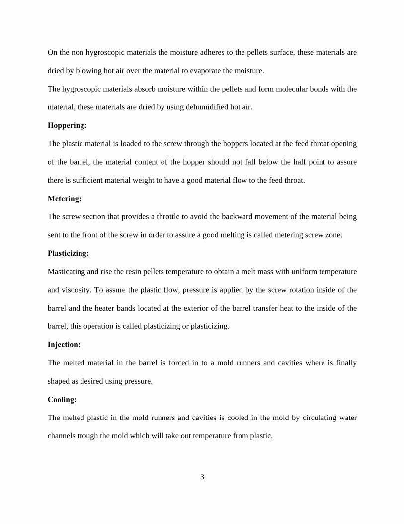
On the non hygroscopic materials the moisture adheres to the pellets surface, these materials are

dried by blowing hot air over the material to evaporate the moisture.

The hygroscopic materials absorb moisture within the pellets and form molecular bonds with the

material, these materials are dried by using dehumidified hot air.

Hoppering:

The plastic material is loaded to the screw through the hoppers located at the feed throat opening

of the barrel, the material content of the hopper should not fall below the half point to assure

there is sufficient material weight to have a good material flow to the feed throat.

Metering:

The screw section that provides a throttle to avoid the backward movement of the material being

sent to the front of the screw in order to assure a good melting is called metering screw zone.

Plasticizing:

Masticating and rise the resin pellets temperature to obtain a melt mass with uniform temperature

and viscosity. To assure the plastic flow, pressure is applied by the screw rotation inside of the

barrel and the heater bands located at the exterior of the barrel transfer heat to the inside of the

barrel, this operation is called plasticizing or plasticizing.

Injection:

The melted material in the barrel is forced in to a mold runners and cavities where is finally

shaped as desired using pressure.

Cooling:

The melted plastic in the mold runners and cavities is cooled in the mold by circulating water

channels trough the mold which will take out temperature from plastic.

Ejection:

The removal of the shaped parts from the mold is made by using ejector pins, which are activated

mechanically by a cylinder to push the parts out of the mold.

Figure 1.1 shows a molding machine.

Figure 1.1 Injection Molding Machine

4

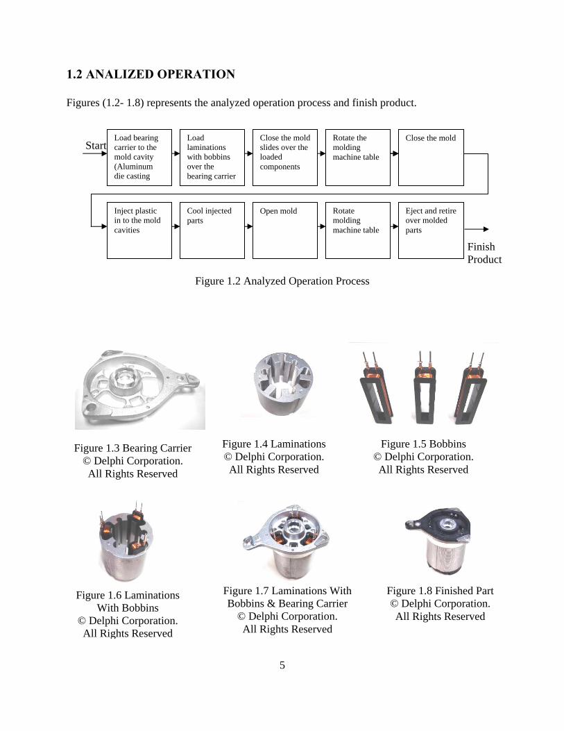
1.2 ANALIZED OPERATION

Figures (1.2- 1.8) represents the analyzed operation process and finish product.

Load bearing carrier to the mold cavity (Aluminum die casting

Load laminations with bobbins over the bearing carrier

Close the mold slides over the loaded components

Rotate the molding machine table

Close the mold

Inject plastic in to the mold cavities

Cool injected parts

Open mold Rotate molding machine table

Eject and retire over molded parts

Start

Finish Product

Figure 1.2 Analyzed Operation Process

Figure 1.5 Bobbins

© Delphi Corporation. All Rights Reserved

Figure 1.4 Laminations © Delphi Corporation. All Rights Reserved

Figure 1.3 Bearing Carrier © Delphi Corporation. All Rights Reserved

Figure 1.8 Finished Part © Delphi Corporation. All Rights Reserved

Figure 1.7 Laminations With Bobbins & Bearing Carrier

© Delphi Corporation. All Rights Reserved

Figure 1.6 Laminations With Bobbins

© Delphi Corporation. All Rights Reserved

5

The finished good part is used as a component to build a Smart Remote Actuator (SRA) “Delphi

Smart Remote Actuators (SRA) are electromechanical devices that actuate engine features, such

as variable geometry turbochargers (VGT) and exhaust gas recirculation (EGR) valves. They

also provide precise rotary position feedback to the engine control unit, which is provided either

by a controlled area network (CAN-protocol), or pulse width modulation (PWM-signal).

Their vibration and temperature resistance capabilities enable Delphi SRA to withstand harsh

environments. Liquid cooling is also available for extremely high temperature environment

applications to protect the brushless motor and the integrated electronics. Integrated electronics

enable software and calibration changes without modification of the electronic control unit's

software algorithm. In un-powered conditions, the actuators will move into a default position.

Figure 1.9 shows a Smart Remote Actuator [4].”

Figure 1.9 Delphi Smart Remote Actuators

© Delphi Corporation. All Rights Reserved

6

7

Because of rigid vibration and temperature requirements on this application it is important to

have a good uniform finish on the part and a stable plastic injection process that can meet the

warranty fulfillments of this part.

1.3 TAGUCHI’S APROACH

Traditional design of experiments is the study of response with the purpose to find an equation

that has a small error, many variables that affect the response characteristic are listed and an

experiment using these variables is conducted.

The equation is written as y=f(M,x1,x2,…,xn)

Where y is the response, M is the input signal and x1,x2,…,xn the noise factors.

The above approach is appropriate for scientific studies, but for engineering studies where the

objective is to develop a good product efficiently at low cost. The Taguchi approach is the most

indicated due to the savings on time, pieces and by consequence the cost, because of the less

number of runs and simplification of the experiment [5].

Taguchi’s proposal is an experimental plan in terms of orthogonal array that provide different

combinations of parameters and their levels. According to this technique we can use minimal

number of experiments to study the entire parameter space. An average of the response variable

is used to perform a main effect analysis [5]. A signal to noise ratio study is perform in order to

have a sensitivity analysis and find out which run have the least variation around the target value

(in this case larger the best is used) [6-8].

8

1.4 PROCESS CAPABILITY INDEX (CPK)

The range that contains all possible values for a quality characteristic is the process capability.

The exact range of these values can be determined only if 100% inspection is conduct. This will

have measuring error and in the majority of the cases, is not feasible or economical. An

alternative to have an estimation of the capability of the process is to take a sample of the values

and use the sample information by expressing the ranges of the values of the probability

distribution as functions of their parameters, especially their standard deviations.

The process capability ratio or Cp compares the engineering tolerance specifications for the

quality characteristic with the process capability and provides an indication of the rejection

percentage. The formulas to calculate the Cp are as follows.

Cp for nominal the best type characteristics =(USL-LSL)/6σ. ………….………………….Eq.1.1

Cp for smaller the best type characteristics = (USL-µ)/3σ………………………..….……..Eq.1.2

Cp for larger the best type characteristics = (µ-LSL)/3σ……………………...…………….Eq.1.3

The formulas for smaller the better and larger the better Cpk, are the same as for the Cp

previously discussed, since we are using only one limit in this case is lower limit [9].

1.5 MOLD FLOW SIMULATION APPROACH

Mold flow is a software that simulate the complicated plastic injection process, provides easy to

use tools that help to optimize the plastic parts. Also other features as runners, cooling channels,

gates and process parameters can be simulate to get an estimated results report. The process

results can be predicted without the use of numerous prototype molds and the waste of

components, raw materials and resources. For digital prototyping, provides easy-to-use tools that

9

simulate and optimize parts, mold, and tool designs this way the number of physical prototypes

required to perfect a design can be reduced.

The used version for the software is 6.0, 64 bit [10].

1.6 PROBLEM DESCRIPTION

In a new model SRA stator over mold process we have encounter assemblies not completely fill

on the part (short shots) due to a poor flow of plastic going through a runner system and cavities

that are in the tool resulting in a high scrap rate due to short shots. The used plastic material is

(polybutylene Terephthalate with 45% glass/mineral reinforcement). It has certain degree of

difficulties to flow due to the glass and mineral content. The operation consists of components

over mold which mean that we need to cover components with plastic and this will cause

difficulties for the plastic to flow due to the size and temperature of the components. The actual

scrap cost due to this condition is about $1000 USD per month. Figures (1.10, 1.11) show a bad

and a good parts.

The analysis experiment was done on a new 85 Ton horizontal injection and vertical clamp

rotary table ENGEL molding machine in a regular production floor to solve a short shot problem

for an SRA stator over mold process. This operation takes three components and plastic resin to

produce a complete stator assembly.

The plastic flow in this mold with the components is particularly difficult for this operation due

to the components temperature and the glass and mineral fibers reinforcement in the plastic resin.

These condition represents a good challenge to optimize the process.

Figure 1.11 Good Part © Delphi Corporation. All Rights Reserved

Figure 1.10 Short Shot Part © Delphi Corporation. All Rights Reserved

1.7 HYPOTHESIS

The use of polybutylene Terephthalate with 45% glass/mineral reinforcement is good for

mechanical and corrosion resistance properties [11]. The correct process for this material is

necessary to maintain the material properties, since several of the process parameters used affects

the material performance. Results from not using optimal parameters are degradation, porosity,

cracks, flow lines, short shots and many other defects on the product that affect properties of the

material [1].

A way to obtain an optimal process is by choosing the correct values for the process parameters.

A good approach to do this is through a Taguchi DOE analysis, which will provide us with a

process optimization even though that components and time availability are constraints that we

have [5].

10

11

Cpk calculation for each run of the experiment was conduct and the results were compared with

the Taguchi’s approach in order to establish if this Cpk approach lead us to similar conclusions.

In this way, the majority of the Industry people can have a better understanding of the results

since Cpk index is used more often to make decisions in the industry.

To determine the parameters to be studied here we will take some references from injection

molding literature [1], previous experiences on conducted (DOE’s) and for the levels, we will

use the recommended in the material data sheet [12]. All of this provides us the guideline on a

good set of parameters and levels to conduct the experiment.

Finally, mold flow software will be used in order to compare the simulation results with the

results from Taguchi approach and use as a reference for future experiments. If the results from

both studies are the same we should see savings on parts, raw material, and machine utilization

for future problem solving in the molding operations.

1.8 THESIS ORGANIZATION

This thesis consists of 5 chapters.

Chapter I: Introduction, Chapter II: Literature Review, Chapter III: Methodology proposal

description, Chapter IV: Results and discussions, Chapter V: Conclusions and recommendations.

12

Chapter II

LITERATURE REVIEW

In September 1999 Qiming Chen and C. Ravindran “A Study of Thermal Parameters and

Interdendritic Feeding in Lost Foam Casting” were published. This article is an example of the

application of an experimental approach to predict results in a final product by modifying the

gate and feeder design of the tool [13].

The main difference between this article and this thesis is that the thesis is considering the

parameters modification instead the tool modifications and this thesis is also considering the Cpk

approach, which is more commonly used in the industry to take decisions.

In 2009 Wen-Chin Chen a, Gong-Loung Fu b,c, Pei-Hao Tai b, Wei-Jaw Deng d, published an

article where Taguchi’s parameter design method were integrated with neural networks, genetic

algorithms and engineering optimization methods to optimize a Molding injection process [14].

This article is using very good tools and obtaining an optimization for the evaluated quality

characteristic. This thesis apply the Cpk approach and running the experiment for an insert

molding which have very different conditions for the evaluated quality characteristic (flow of the

material inside the mold) also the reinforced material represents a difficulty to flow.

13

G. Toselloa, A. Gavab, H.N. Hansena, G. Lucchetta b, F. Marinellob published an article where

DOE were used to minimize the weld lines on a finished product [15].

Other related article was published by Xuehong Lu and Lau Soo Khim, where experiments were

performed in order to optimize the quality for an optical lens, by modifying the injection molding

process parameters [16].

These articles are closer from what we did on this thesis due to weld lines and part quality are

related to the material flow inside the mold.

This thesis is also covering the Cpk approach and using a simulation software to correlate with

the DOE and Cpk approaches. The simulation is validated with scientific evidence and can be

freely used to optimize the process without use any components, machine time and operator

resources, providing big savings.

In general, the main difference between these articles and this thesis is that this thesis is

establishing a bridge between the scientific approaches (DOE Taguchi, Cpk) and the simulation

approach. This is leading us to have more savings on resources and time.

Also the quantity of prototype molds and modifications to these molds to obtain an optimal

finish part is smaller due to the use of simulation software.

14

Chapter III

METHODOLOGY PROPOSSAL DESCRIPTION

3.1 TAGUCHI APPROACH

3.1.1 RESPONSE VARIABLE ESTABLISHMENT

Response variable was established by using the product characteristic that need to be optimized

to avoid certain defect or to have an improvement of the quality. In this case, the defect is short

shot, then the filling quality of the part is used as the response variable. The weight of the parts is

an indicator of the quality of the parts filling then the weight is used as a response variable the

heaviest part is a good part and the lightest part is the worst part. Weights were measured with a

digital scale with 1-gram resolution, serial number: 1204230 and Cal due date: March/2010.

3.1.2 SELECTION OF PARAMETERS AND THEIR LEVELS

In order to solve a fault in a molded product we can focus on 6 topics

1. Machine, 2. Molds, 3. Operating conditions (time, temperature, pressure), 4. Material,

5. Part design, 6. Management

Due to the part design stage is already ended, we have a new machine with good capability to

over mold these parts, the molds build is finish, the material were chosen due to its mechanical

and dimensional stability. We will focus on the operation conditions (time, temperature and

pressure) parameters. The time is related to the time to fill the part we will use Injection speed,

temperature is related to the barrel temperature and we will use the barrel temperature profile,

and pressure is related to the injection pressure that we will use as a factor [1]

15

These factors are also chosen from literature that shows these factors are the most significant for

injection molding process [2,14,15] and by taking in consideration the experience with

previously performed experiments for Injection molding process. The number of levels are three

in order to evaluate the parameters for the actual condition and lower and upper side. No

resources were available to make extended experiment.

3.1.3 SELECTION OF ORTOGONAL ARRAY

The orthogonal array must be selected according to the degrees of freedom from the parameters;

the number of runs for the Taguchi’s experiment must be greater or at least equal to the number

of degrees of freedom for the parameters.

Degrees of freedom for the parameters are as follows:

3 parameters with 3 levels each then the degrees of freedom for each parameter is two, three

parameters with two degrees of freedom each make a total of 6 degrees of freedom, then is good

to select a L9 (nine runs) array to perform the Taguchi’s experiment [6].

3.1.4 ANALYSIS OF THE RUNS RESULTS

The analysis of the results from the runs is performed using Minitab statistical software.

Obtaining the main effects charts for means and signal to noise ratios to know which level is

better to use to have good results for the response variable. The requested analysis is bigger the

best. Finally, a confirmation run is performed using the optimal parameters values. Which is

obtained from the previous analysis.

Cpk Index is calculated to compare with the Taguchi’s approach results and evaluate if they are

well with each other.

16

3.2 CPK APPROACH

Cpk approach is an ideal index to indicate process capability and can be used to estimate the

proportion of defectives. Also contain information about the distances between the mean and the

specification limits, upper specification and lower specification, the value to choose would be the

minimum of both distances since the minimum will represents the worst case in terms of

proportion defectives.

The Cpk for characteristics with only one specification limit (smaller the better and larger the

better type) is the same as the Cp index.

3.2.1 CPK CALCULATIONS

Equation 1.3 is applied to calculated the Cpk for this case due to only the lower limit is present

for this product. This is the same formula used to calculate the Cp index.

The lower specification limit (LSL) for this case is 330 grams which is the lower value for the

weight of the pieces that shows good condition for finished parts.

3.2.2 CPK RESULTS INTERPRETATION

For normal applications of this approach a 1.67 Cpk value is a good indicator for process

capability. In this case the Cpk values are lower than this specification due to the nature of the

evaluated quality characteristic and we choose the higher value since the higher value is a better

result.

17

3.3 MOLD FLOW ANALYSIS

Mold flow analysis is performed to compare results from Taguchi approach and obtain a good

base to say that we can use this approach to make future experiments to save components, time

and resources.

This approach requires an IGS solid file with no radiuses and no blends also all the internal

components must be removed that is obtained from design department.

The solid is imported from the source by using the import feature of the software.

After the importation of the solid a mesh is generated on the solid, this will create a triangle

mesh on the solid surfaces; this is performed by using the Mesh icon on the software.

After the mesh generation a treatment of the solid to fix the majority of the errors in the solid that

can effect the final result of the analysis is performed by the usage of the repair wizard icon on

the software. Finally a projection operation is performed in order to put back to the surface of the

solid all the moved nodes due to the fixing operations.

To make the analysis of the plastic injection process on this software is necessary to include the

most information that we have from the process, Machine, Material, cooling channels, runners

and injection gates characteristics and parameters values by using the proper icons and galleries

existents on the software.

Finally the Analyze now icon is used to perform the analysis.

CHAPTER IV

RESULTS AND DISCUSSIONS

4.1 TAGUCHI APPROACH

4.1.1 RESPONSE VARIABLE ESTABLISHMENT

As were explained before on 3.1.1 the response variable was established by the filling quality of

the part parts were weighted and weights from 324 to 332 grams were obtained being the worst

condition the parts with 324 grams and the acceptable condition with 330 and 332 grams.

The weight values obtained are 324g, 326g, 330g and 332g

The following pictures show the parts for the best and worst conditions.

WOW Piece BOB Piece

Figure 4.1 Worst And Best Case Pieces

WOW (Worst of Worst), BOB (Best of Best).

The most extreme parts from a sample (Worst and Best).

18

19

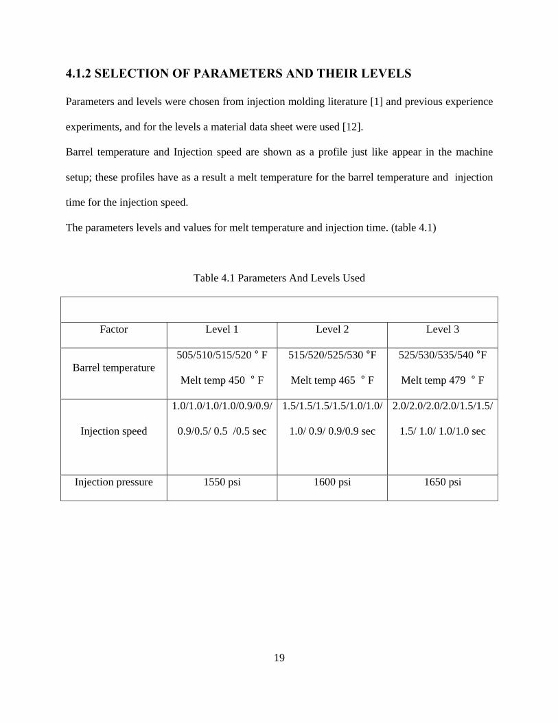
4.1.2 SELECTION OF PARAMETERS AND THEIR LEVELS

Parameters and levels were chosen from injection molding literature [1] and previous experience

experiments, and for the levels a material data sheet were used [12].

Barrel temperature and Injection speed are shown as a profile just like appear in the machine

setup; these profiles have as a result a melt temperature for the barrel temperature and injection

time for the injection speed.

The parameters levels and values for melt temperature and injection time. (table 4.1)

Table 4.1 Parameters And Levels Used

Factor Level 1 Level 2 Level 3

Barrel temperature 505/510/515/520 ° F

Melt temp 450 ° F

515/520/525/530 °F

Melt temp 465 ° F

525/530/535/540 °F

Melt temp 479 ° F

Injection speed

1.0/1.0/1.0/1.0/0.9/0.9/

0.9/0.5/ 0.5 /0.5 sec

1.5/1.5/1.5/1.5/1.0/1.0/

1.0/ 0.9/ 0.9/0.9 sec

2.0/2.0/2.0/2.0/1.5/1.5/

1.5/ 1.0/ 1.0/1.0 sec

Injection pressure 1550 psi 1600 psi 1650 psi

20

4.1.3 SELECTION OF ORTOGONAL ARRAY

Experiment had three parameters with three levels each. This mean that there is 2 degrees of

freedom for each parameter then the sum of the tree parameters degrees of freedom is 6 and the

total of degrees of freedom for the entire experiment is 6, an orthogonal array with more or at

least 6 runs is needed for Taguchi’s approach.

Minitab statistical software is used to generate a L9 orthogonal array; this will cover the

requirements from the degrees of freedom standpoint also a table with the parameters levels for

each run is provided to run the experiment without any errors.

Tables 4.2 and 4.3 show the array and the runs with the parameters levels to use.

Table 4.2 L9 Array For Taguchi’s Approach Generated With Minitab Statistical Software

Run Barrel temperature Injection speed Max Injection Pressure

1 1 1 1

2 1 2 2

3 1 3 3

4 2 1 2

5 2 2 3

6 2 3 1

7 3 1 3

8 3 2 1

9 3 3 2

21

Table 4.3 L9 Array With Level Values For The Parameters

Run Barrel temperature Injection speed Max Injection

Pressure Injection Time

1 505/510/515/520 °

F 1.0/1.0/1.0/1.0/0.9/0.9/ 0.9/0.5/0.5/0.5

sec 1550 psi 4.495 sec

2 505/510/515/520 °

F 1.5/1.5/1.5/1.5/1.0/1.0/ 1.0/ 0.9/0.9/0.9

sec 1600 psi 4.237 sec

3 505/510/515/520 °

F 2.0/2.0/2.0/2.0/1.5/1.5/ 1.5/ 1.0/1.0/1.0

sec 1650 psi 4.437 sec

4 515/520/525/530

°F 1.0/1.0/1.0/1.0/0.9/0.9/ 0.9/0.5/0.5/0.5

sec 1600 psi 3.453 sec

5 515/520/525/530

°F 1.5/1.5/1.5/1.5/1.0/1.0/ 1.0/ 0.9/0.9/0.9

sec 1650 psi 2.832 sec

6 515/520/525/530

°F 2.0/2.0/2.0/2.0/1.5/1.5/ 1.5/ 1.0/1.0/1.0

sec 1550 psi 2.952 sec

7 525/530/535/540

°F 1.0/1.0/1.0/1.0/0.9/0.9/ 0.9/0.5/0.5/0.5

sec 1650 psi 2.235 sec

8 525/530/535/540

°F 1.5/1.5/1.5/1.5/1.0/1.0/ 1.0/ 0.9/ .9/0.9

sec 1550 psi 2.289 sec

9 525/530/535/540

°F 2.0/2.0/2.0/2.0/1.5/1.5/ 1.5/ 1.0/1.0/1.0

sec 1600 psi 2.073 sec

4.1.4 ANALYSIS OF THE RUNS RESULTS

The pieces that came out from the experiment runs were marked with three numbers the first

number is the run number, the second number is the cavity number and the third number is the

sample number, the results for weights are shown in table 4.4.

22

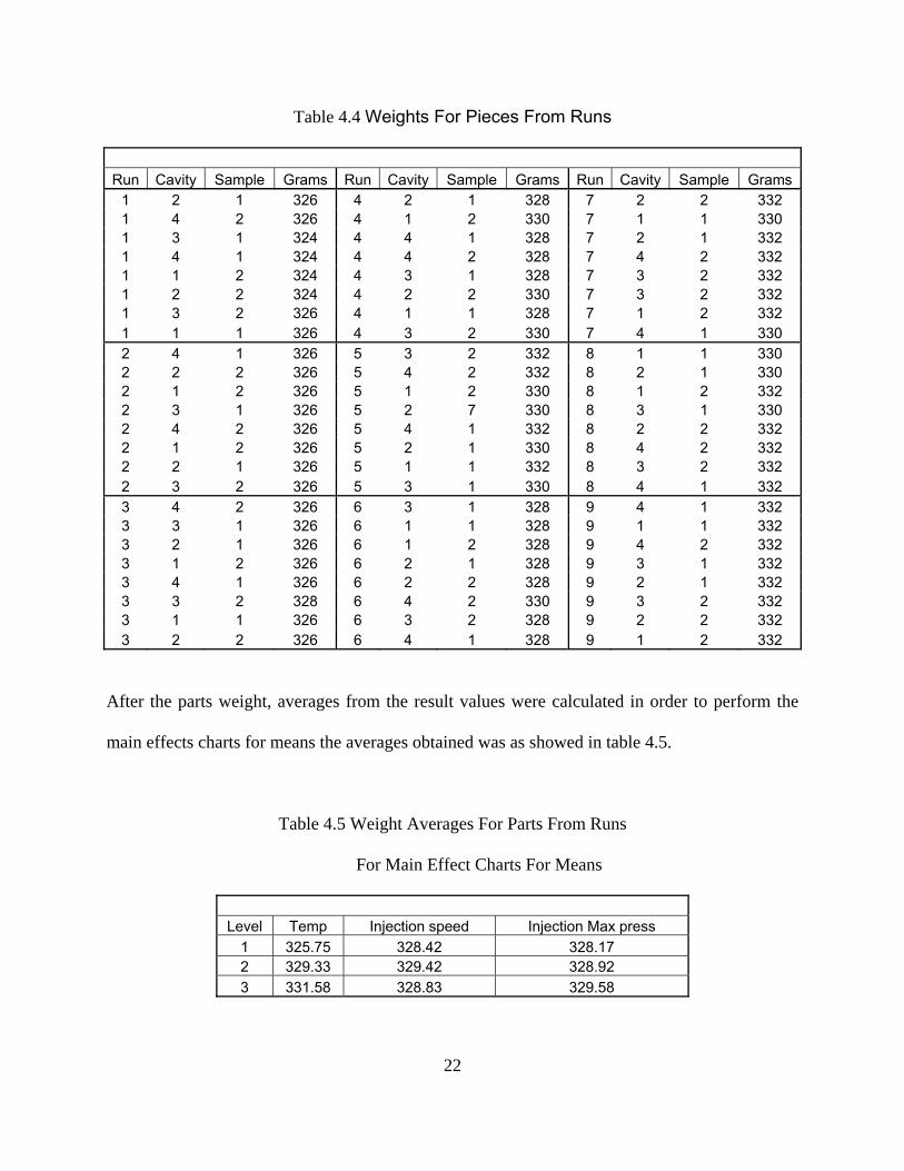
Table 4.4 Weights For Pieces From Runs

Run Cavity Sample Grams Run Cavity Sample Grams Run Cavity Sample Grams

1 2 1 326 4 2 1 328 7 2 2 332 1 4 2 326 4 1 2 330 7 1 1 330 1 3 1 324 4 4 1 328 7 2 1 332 1 4 1 324 4 4 2 328 7 4 2 332 1 1 2 324 4 3 1 328 7 3 2 332 1 2 2 324 4 2 2 330 7 3 2 332 1 3 2 326 4 1 1 328 7 1 2 332 1 1 1 326 4 3 2 330 7 4 1 330 2 4 1 326 5 3 2 332 8 1 1 330 2 2 2 326 5 4 2 332 8 2 1 330 2 1 2 326 5 1 2 330 8 1 2 332 2 3 1 326 5 2 7 330 8 3 1 330 2 4 2 326 5 4 1 332 8 2 2 332 2 1 2 326 5 2 1 330 8 4 2 332 2 2 1 326 5 1 1 332 8 3 2 332 2 3 2 326 5 3 1 330 8 4 1 332 3 4 2 326 6 3 1 328 9 4 1 332 3 3 1 326 6 1 1 328 9 1 1 332 3 2 1 326 6 1 2 328 9 4 2 332 3 1 2 326 6 2 1 328 9 3 1 332 3 4 1 326 6 2 2 328 9 2 1 332 3 3 2 328 6 4 2 330 9 3 2 332 3 1 1 326 6 3 2 328 9 2 2 332 3 2 2 326 6 4 1 328 9 1 2 332

After the parts weight, averages from the result values were calculated in order to perform the

main effects charts for means the averages obtained was as showed in table 4.5.

Table 4.5 Weight Averages For Parts From Runs

For Main Effect Charts For Means

Level Temp Injection speed Injection Max press

1 325.75 328.42 328.17 2 329.33 329.42 328.92 3 331.58 328.83 329.58

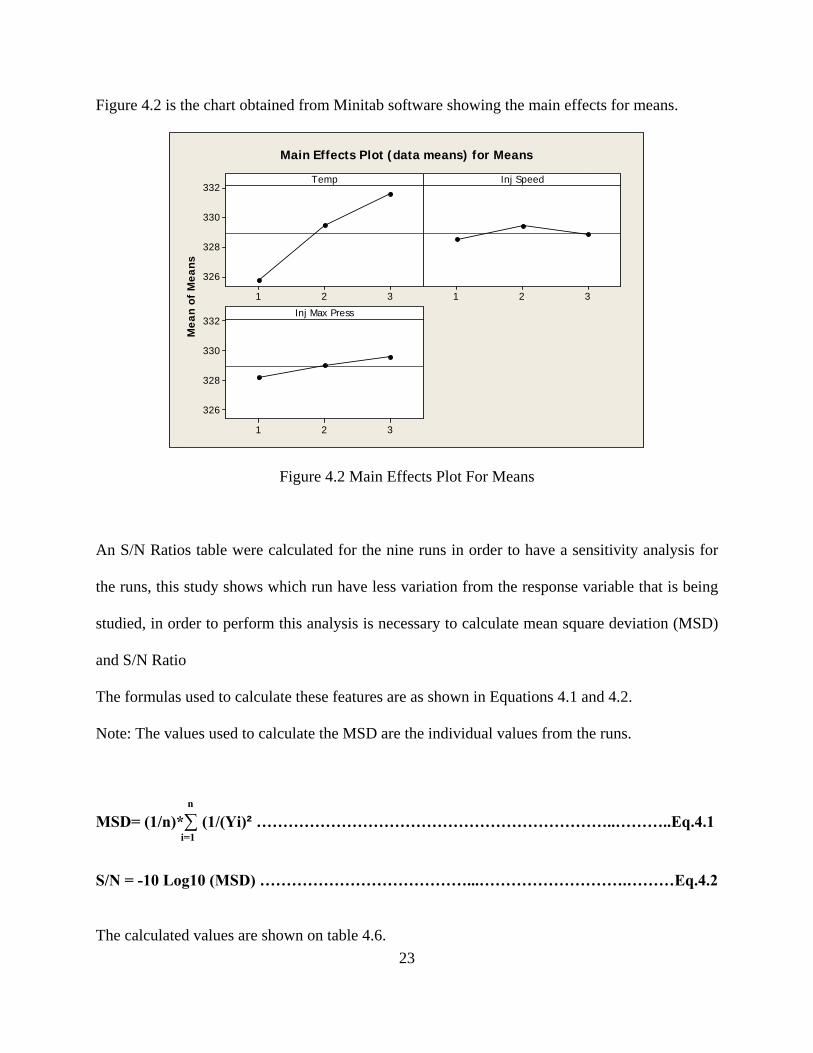
Figure 4.2 is the chart obtained from Minitab software showing the main effects for means.

Mea

n of

Mea

ns

321

332

330

328

326

321

321

332

330

328

326

Temp Inj Speed

Inj Max Press

Main Effects Plot (data means) for Means

Figure 4.2 Main Effects Plot For Means

An S/N Ratios table were calculated for the nine runs in order to have a sensitivity analysis for

the runs, this study shows which run have less variation from the response variable that is being

studied, in order to perform this analysis is necessary to calculate mean square deviation (MSD)

and S/N Ratio

The formulas used to calculate these features are as shown in Equations 4.1 and 4.2.

Note: The values used to calculate the MSD are the individual values from the runs.

n

MSD= (1/n)*∑ (1/(Yi)² …………………………………………………………..………..Eq.4.1 i=1 S/N = -10 Log10 (MSD) …………………………………...……………………….………Eq.4.2 The calculated values are shown on table 4.6.

23

24

Table 4.6 MSD And S/N Ratios Calculation

Run Average weight MSD S/N Ratios

1 325.0000 9.46772E-06 50.24 2 326.0000 9.40946E-06 50.26 3 326.2500 9.39516E-06 50.27 4 328.7500 1.0387E-05 49.84 5 331.0000 9.12759E-06 50.40 6 328.2500 9.28102E-06 50.32 7 331.5000 9.10001E-06 50.41 8 331.2500 9.11380E-06 50.40 9 332.0000 9.07243E-06 50.42

Averages from S/N ratios for the factor levels are shown on table 4.7.

Table 4.7 S/N Ratios Averages For Parts From Runs

For Main Effect Charts For S/N Ratios

Level Temp Injection speed Injection Max press

1 50.26 50.16 50.32 2 50.19 50.35 50.17 3 50.41 50.34 50.36

We can observe that the best level value for Temp is 3 with an S/N ratio value of 50.41, for

Injection speed is level 2 with an S/N ratio value of 50.35 and for Injection Max press is level 3

with an S/N ratio value of 50.36.

Table 4.8 shows the best parameter levels according to Taguchi’s approach.

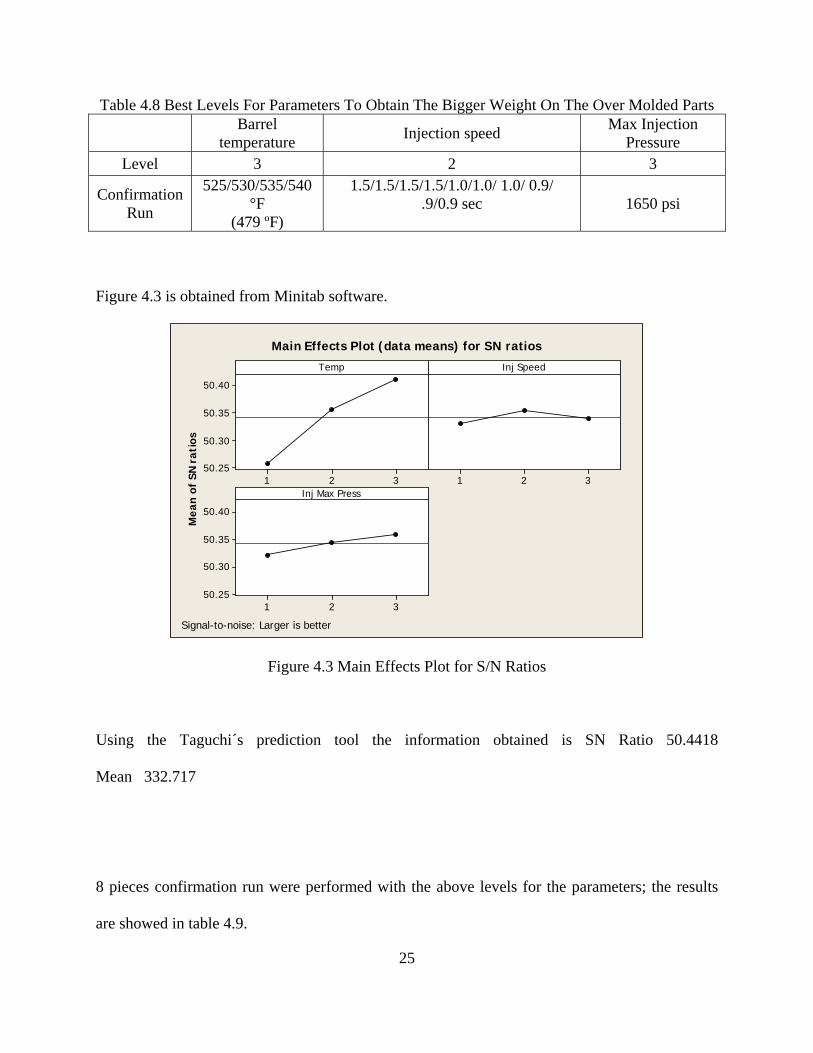
Table 4.8 Best Levels For Parameters To Obtain The Bigger Weight On The Over Molded Parts

Barrel temperature Injection speed Max Injection

Pressure Level 3 2 3

Confirmation Run

525/530/535/540 °F

(479 ºF)

1.5/1.5/1.5/1.5/1.0/1.0/ 1.0/ 0.9/ .9/0.9 sec

1650 psi

Figure 4.3 is obtained from Minitab software.

Mea

n of

SN

rati

os

321

50.40

50.35

50.30

50.25321

321

50.40

50.35

50.30

50.25

Temp Inj Speed

Inj Max Press

Main Effects Plot (data means) for SN ratios

Signal-to-noise: Larger is better

Figure 4.3 Main Effects Plot for S/N Ratios

Using the Taguchi´s prediction tool the information obtained is SN Ratio 50.4418

Mean 332.717

8 pieces confirmation run were performed with the above levels for the parameters; the results

are showed in table 4.9.

25

26

Table 4.9 Confirmation Run Results

Confirmation Run Cav Sample Weight

4 1 332 grams 1 1 332 grams 4 2 332 grams 3 1 332 grams 2 1 332 grams 3 2 332 grams 2 2 332 grams 1 2 332 grams

The confirmation run approves the results from Taguchi’s approach and give us optimal finished

good parts with a weight of 332g and no variation, since the same results are obtain from run

number 9 then we will use run number 9 for Cpk calculations approach, this will lead us to the

same Cpk results and for Mold flow approach we will use run number 9 to avoid apply excessive

pressure that contribute to the machine wear.

All the cavities have a weight of 332 g using the optimal setup, this condition indicate that there

is no difference between cavities.

27

4.2 CPK APPROACH

4.2.1 CPK CALCULATIONS

In order to calculate the CPK Equation 1.3 were used. The lower limit to use in this equation is

330g

Cpk for larger the best type characteristics = (µ-LSL)/3σ, from Eq.1.3

Table 4.10 shows the CPK values obtained for the 9 experiment runs.

Table 4.10 CPK Values For The 9 Experiment Runs

CPK Values for the 9 experiment runs

RUN CPK Value 1 -1.56 2 ≈ - ∞ 3 -1.77 4 -0.40 5 0.31 6 -0.82 7 0.54 8 0.40 9 ≈ ∞

4.2.2 CPK RESULTS INTERPRETATION

The CPK’s with a negative value are definitively bad result and for this case we can choose the

one with the bigger value and those are run number 9 that tends to be infinity. Run 7 with 0.54

and run 8 with 0.40.

Then we can choose run number 9 as the best result.

We can appreciate that Cpk results capture standard deviation, mean location and variation

between data of the same run, this variation is captured by the MSD calculation on Taguchi’s

approach.

4.3 MOLD FLOW ANALYSIS

4.3.2 SOLID IMPORTATION AND TREATMENT

The first step to process the solid is generating a mesh that will create a layer of triangles on the

solid surface and these triangles will serve as the walls of the plastic part to simulate the process

Figures 4.4 and 4.5 shows this step.

Figure 4.4 Generating Mesh

28

Figure 4.5 Solid With Mesh

After the mesh generation a mesh repair wizard is performed to correct any errors occurred

during the mesh generation, mesh repair step is showed in figure 4.6.

Figure 4.6 Mesh Repair

29

Once the repair is done, a mesh diagnostics aspect ratio is performed in order to repair the solid

if needed, the size of the triangles must be 6 mm. Aspect ratio step is showed in figure 4.7.

Figure 4.7 Aspect Ratio

Once the repair is done, a mesh statistics is performed in order to evaluate if the solid is ready to

run the simulation and if not a reparation of the solid is needed, figure 4.8 shows Mesh statistics

test step.

Figure 4.8 Mesh Statistics

30

The mesh statistics test result must give an 87% value to indicate the solid is finally ready to run

the simulation.

Note: In order to get a good conformance of the solid the design department support was needed.

4.3.3 MOLD FLOW ANALYSIS RUN

In order to perform the analysis is necessary to specify the mold gates location, cooling channels,

material used, machine used, process parameters.

All the above are available in the software libraries, and setup input is performed in the process

settings area, figures (4.9 – 4.11) shows model and menus to load the above information to the

model.

Figure 4.9 Model To Simulate

31

Figure 4.10 Process Settings Screens

32

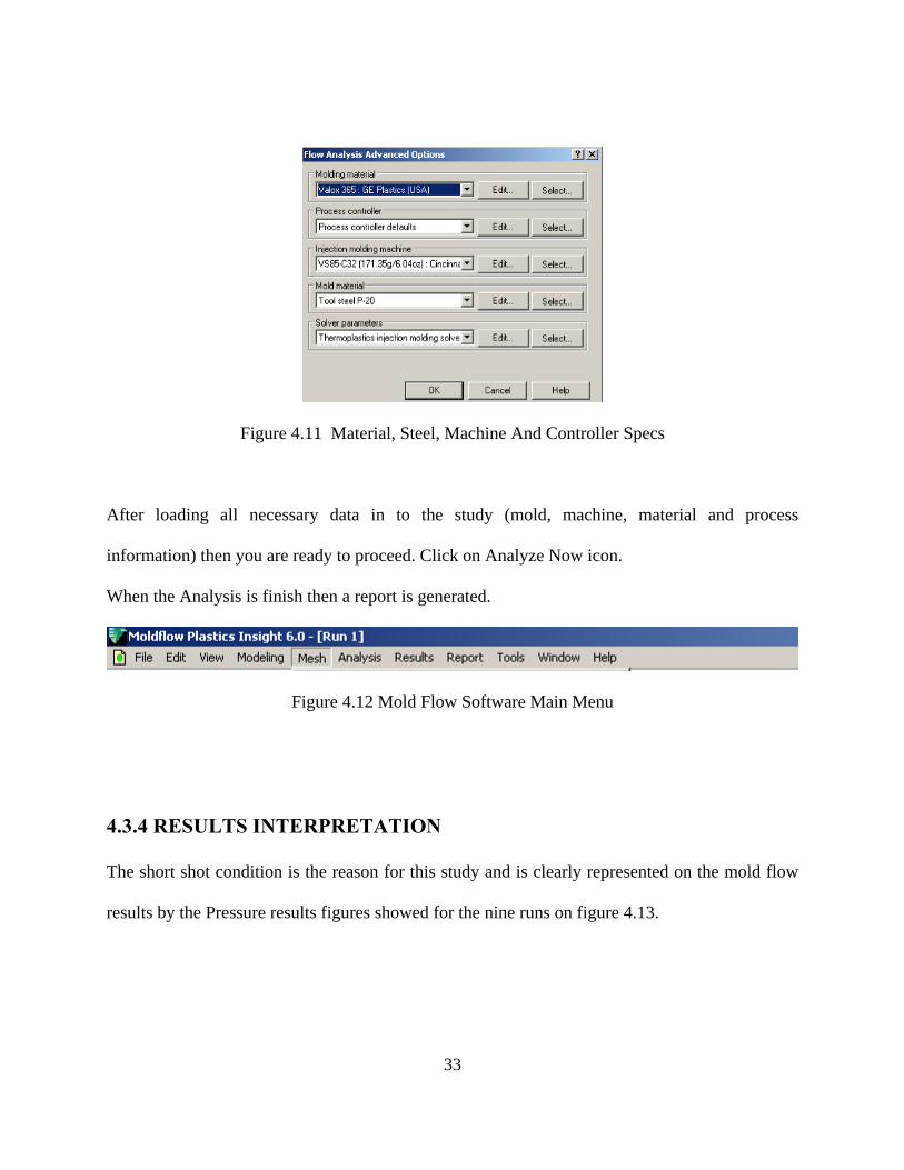
Figure 4.11 Material, Steel, Machine And Controller Specs

After loading all necessary data in to the study (mold, machine, material and process

information) then you are ready to proceed. Click on Analyze Now icon.

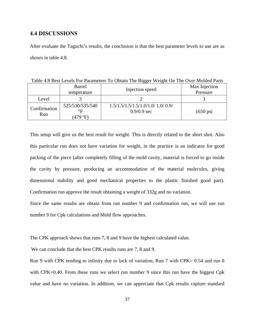
When the Analysis is finish then a report is generated.

Figure 4.12 Mold Flow Software Main Menu

4.3.4 RESULTS INTERPRETATION

The short shot condition is the reason for this study and is clearly represented on the mold flow

results by the Pressure results figures showed for the nine runs on figure 4.13.

33

Run 1 Run 2 Run 3

34

Figure 4.13 9 Runs Pressure Comparison

By looking at the above figures, it is clear that runs 7, 8, 9 are the best in filling. The remaining

runs will produce a short shot condition. These results correlate well with the Taguchi and CPK

Studies.

Run 4 Run 5 Run 6

Run 7 Run 8 Run 9

Then a comparison of the filling times is performed to evaluate which of the good runs is better,

figures (4.14 - 4.16) shows the different filling times for runs 7, 8 and 9.

Figure 4.14 Run 7 Filling Time

Figure 4.15 Run 8 Filling Time

35

Figure 4.16 Run 9 Filling Time

After comparing the fill time, on the figures run 7 through 9. It has been determine that run

number 9 is the best out of all them. Reason for this selection, is the uniform plastic layers being

display by figure 4.16 and the fill time of 2.075 seconds. This results correlate with the Taguchi

and CPK studies. This will allow us to have better dimensional parts, of course that there are

other parameters included, but the main one we are looking at is fill time.

36

37

4.4 DISCUSSIONS

After evaluate the Taguchi’s results, the conclusion is that the best parameter levels to use are as

shown in table 4.8.

Table 4.8 Best Levels For Parameters To Obtain The Bigger Weight On The Over Molded Parts

Barrel temperature Injection speed Max Injection

Pressure Level 3 2 3

Confirmation Run

525/530/535/540 °F

(479 ºF)

1.5/1.5/1.5/1.5/1.0/1.0/ 1.0/ 0.9/ 0.9/0.9 sec

1650 psi

This setup will give us the best result for weight. This is directly related to the short shot. Also

this particular run does not have variation for weight, in the practice is an indicator for good

packing of the piece (after completely filling of the mold cavity, material is forced to go inside

the cavity by pressure, producing an accommodation of the material molecules, giving

dimensional stability and good mechanical properties to the plastic finished good part).

Confirmation run approve the result obtaining a weight of 332g and no variation.

Since the same results are obtain from run number 9 and confirmation run, we will use run

number 9 for Cpk calculations and Mold flow approaches.

The CPK approach shows that runs 7, 8 and 9 have the highest calculated value.

We can conclude that the best CPK results runs are 7, 8 and 9.

Run 9 with CPK tending to infinity due to lack of variation, Run 7 with CPK= 0.54 and run 8

with CPK=0.40. From these runs we select run number 9 since this run have the biggest Cpk

value and have no variation. In addition, we can appreciate that Cpk results capture standard

38

deviation, mean location and also variation between data of the same run, this variation is

captured by the MSD calculation on Taguchi’s approach and the results between Taguchi’s

approach and Cpk approach correlates well.

The Mold flow indicates that runs 7, 8 are also acceptable, but run 9 being the best. Even though

7 & 8 are acceptable, run 9 was chosen because of the fill time.

Run 9 takes 2.073 seconds to fill the part, Run 7 is a little bit longer 2.236 seconds to fill the part

and run 8 takes 2.289 seconds to fill the part. Shorter filling time is better; due to this allow more

material to go in the mold cavities.

Once the tree approaches are compared the conclusion is the same, the best run to use is run 9

followed by run 7 and 8, confirmation run looks like better than run number 9 for Taguchi

approach but for this particular process we obtain the same results with run number 9 and

confirmation run and is better to use the run with less pressure applied to avoid machine and

mold wear.

39

CHAPTER V

CONCLUSIONS AND RECOMENDATIONS

We can conclude that, by using the available tools at hand it is better than trial and error in trying

to establish a process setup. The entire study must be reviewed before establish an optimum

setup.

Mold Flow is a very good tool to predict the injection molding results before start to build the

mold and without use any components, materials and resources. This is the recommended

approach when resources and money are not available.

This approach reduces the quantity of prototype molds and modifications to these molds to

obtain a finished good part. The limitation to use this software is the treatment of the solid that

will require the expertise of a design Engineer to manipulate the solid in order to make it usable

for the software.

Recommendation is to use run 9 setup.

We recommend obtaining license for the optimization software interface for mold flow software

in order to establish if this software can eliminate the simulation of several runs to optimize the

process. This software will establish a set of parameters that will be optimal by the modification

of more parameters and not only three.

40

REFERENCES

[1] Dominick V. Rosato and, Donald V. Rosato (1985), Injection molding Handbook, Van

Nostrand Reinhold Company, New York

[2] Sanjay Kumar Nayak, and Smita Mohanty (2009), Sisal Glass Fiber Reinforced PP Hybrid

Composites: Evaluation of Dynamic Mechanical and Thermal Properties, Journal of Reinforced

Plastics and Composites, doi:10.1177/0731684409337632

[3] Ruhul A. Khan, and Mubarak A Khan, and Haydar U Zaman, and Shamim Pervin, and

Nuruzzaman Khan, and Sabrina Sultana, and M. Saha, and A. I. Mustafa (2009), Comparative

Studies of Mechanical and Interfacial Properties Between Jute and E-glass Fibers Reinforced

Polypropylene Composites, Journal of Reinforced Plastics and Composites,

doi:10.1177/0731684409103148

[4] http://delphi.com/shared/pdf/ppd/pwrtrn/dsl_smtremote.pdf, Delphi’s website

[5] Genichi Taguchi, and Subir Choudhury, and Yuin Wu (2004), Taguchi’s Quality

Engineering Handbook, ASI Consulting Group, LLC, Livonia, Michigan

[6] S. Kamaruddin, and Zahid A. Khan, and K. S. Wan (2004), The Use Of The Taguchi Method

In Determining The Optimum Plastic Injection Moulding Parameters For The Production Of a

Consumer Product, Jurnal Mekanikal, Volume18 , pp 98 – 110

[7] Babur Ozcelik, and Tuncay Erzurumlu (2005), Determination of Effecting Dimensional

Parameters on Warpage of Thin Shell Plastic Parts Using Integrated Response Surface Method

And Genetic Algorithm, International Communications in Heat and Mass Transfer Journal,

Volume 32, Issue 8, pp 1085-1094

41

[8] Mirigul Altan (2009), Reducing Shrinkage in Injection Moldings Via the Taguchi, ANOVA

and Neural Network Methods, Materials & Design Journal, Accepted Manuscript, Available

online

[9] M. Jeya Chandra (2001), Statistical Quality Control, Boca Raton London New York

Washington, D.C.

[10] http://www.moldflow.com/stp/english/products/autodesk_moldflow_adviser.php, Mold

Flow Website

[11] Macromedia Inc, GE Engineering Thermoplastics Product Wide, Version 7.0.2.85,

Processing section

[12] GE advanced Materials Plastics, Valox 736 Data sheet (now SAVIC)

[13] Qiming Chen C., and Ravindran (2000), A Study of Thermal Parameters and Interdendritic

Feeding in Lost Foam Casting, Journal of Materials Engineering and Performance, Volume 9(4),

pp 386-395

[14] Wen-Chin Chen a, and Gong-Loung Fu b, and Pei-Hao Tai b, and Wei-Jaw Deng d (2009),

Process parameter optimization for MIMO plastic injection molding via soft computing, Elsevier

Expert Systems with Applications Journal, Volume 36, pp1114–1122

[15] G. Toselloa, and A. Gavab, and H.N. Hansena, and G. Lucchetta b, and F. Marinellob

(2008), Characterization and analysis of weld lines on micro-injection moulded parts using

atomic force microscopy (AFM), WEAR Journal, Volume 266, pp 534-538

[16] Xuehong Lu, and Lau Soo Khim (2001), A statistical experimental study of the injection

molding of optical lenses, Journal of Reinforced Plastics and Composites, Vol. 27, No. 8, pp 819-834

42

CURRICULUM VITA

Israel Sanchez was born in Mexico D.F. The first son of Eduardo Sanchez and Eunice Urbina, he

graduated from CBTIS 128 High School, Juarez, Mexico, in the spring of 1992 and entered The

Universdad Autonoma de Ciudad Juarez.

While pursuing a bachelor’s degree in Industrial Engineering, he worked with Kendall

(Manufacture of medical products) from July/99 to February/01. Later he worked with

Molten Mexicana (Manufacture of automotive products) From February/7/2001 to

February/2/2004. And later worked with DELPHI AUTOMOTIVE SYSTEMS (Manufacture of

automotive products for North America) From February/2/2004, and continue Presently

employed with the company, he entered the Graduate School at The University of Texas at El

Paso in the Spring 2007.

Permanent Address: 1951-3 Hacienda la Cantera Juarez Mexico