optimization of geographic map projections for canadian...
TRANSCRIPT

OPTIMIZATION OF GEOGRAPHIC MAP PROJECTIONS
t FOR
CANADIAN TERRITORY
by
Kresho Frank ich
Dip l . Ing . , Geode t i c U n i v e r s i t y of Zagreb, 1959
M.A.Sc., U n i v e r s i t y of B r i t i s h Columbia, 1974
A T h e s i s Submit ted i n P a r t i a l F u l f i l l m e n t
of t h e Requirements f o r t h e Degree of
Doctor of Ph i losophy
by
S p e c i a l Arrangements
c Kresho Frank ich 1982
Simon F r a s e r U n i v e r s i t y
November, 1982
A l l r i g h t s r e s e r v e d . T h i s t h e s i s may n o t be reproduced i n whole o r i n p a r t , by photocopy
o r o t h e r means, w i t h o u t p e r m i s s i o n of t h e a u t h o r .

APPROVAL
Name : Kresho F ' rankich
Degree: Doctor o f P h i l o s o p h y
T i t l e o f T h e s i s : O p t i m i z a t i o n of Geograph ic Map P r o j e c t i o n f o r Canadian T e r r i t o r y
Examining C o m m i t t e e :
C h a i r p e r s o n :
D r . Thomas P o i k e r
- D r . R o b e r t R u s s e l l
D r . A r t h u r R o b e r t s
D r . Hwarlfi r a k i w s k y E x t e r n a l Ex f m i n e r 1 The U n i v e r s i t y o f C a l g a r y
March 3 , 1 9 5 3 Date Approved:

PARTIAL COPYRIGHT LICENSE
I hereby g r a n t t o Simon Fraser U n i v e r s i t y t h e r i g h t t o lend
my t h e s i s , p r o j e c t o r extended essay ( t h e t i t l e o f which i s shown below)
t o users o f t h e Simon Fraser U n i v e r s i t y L i b ra r y , and t o make p a r t i a l o r
s i n g l e cop ies o n l y f o r such users o r i n response t o a reques t f rom t h e
l i b r a r y o f any o t h e r u n i v e r s i t y , o r o t h e r educa t iona l i n s t i t u t i o n , on
i t s own beha l f o r f o r one o f i t s users. I f u r t h e r agree t h a t permiss ion
f o r m u l t i p l e copy ing o f t h i s work f o r s c h o l a r l y purposes may be g ran ted
by me o r t h e Dean o f Graduate Stud ies. I t i s understood t h a t copy ing
o r p u b l i c a t i o n o f t h i s work f o r f i n a n c i a l g a i n s h a l l n o t be a l lowed
w i t h o u t my w r i t t e n permiss ion.
T i t l e o f Thes is /Pro ject /Extended Essay
Author:
( s i g n a t u r e )
( name

iii
I
ABSTRACT
One of the main tasks of mathematical cartography is to
determine a projection of a mapped territory in such a way that
the resulting deformations of angles, areas and distances are
objectively minimized. Since the transformation process will
generally change the original distances it is appropriate to
adopt the deformation of distances as the basic parameter for
the evaluation of map projections. As the qualitative measure
of map projections the author decided to use the Airy-
Kavraiskii criterion
where A is the area of the mapping domain, a and b semi-axes of
the indicatrix of Tissot, and the integration is extended to
the whole domain. Until now all optimization of map projec-
tions were referred to domains with analytically defined
boundaries, for example, a spherical trapezoid, spherical cap
or a hemisphere, and for those map projections in which the
analytical evaluation of the integral was possible. The author
expands the optimization process to irregular domains with
boundaries consisting of a series of discrete points. The
minimization of the criterion leads to a least square
adjustment problem.

I
The main purpose of the project was to develop a uniform
method to optimize the standard and most frequently used
mapping systems in geography for Canadian territory. The scope
of optimization was enlarged by the inclusion of the
optimization of modified equiareal projections as well as the
determination of the Chebyshev conformal projections.
Almost all small scale maps of the territory of Canada
have been based on the normal aspect of the Lambert Conformal
Conic projection with standard parallels at latitudes of 49'
and 77". Every optimized projection in the research yielded a
smaller value for the Airy-Kavraiskii criterion. Thus, it was
proven that any standard map project ion with properly selected
metagraticule and constant parameters of the projection is much
better than the official projection. The best result was
achieved with the optimized equidistant projection. Since the
projection equations for the equidistant conic projection are
very simple and the projection gives the best result with
respect to the Airy-Kavraiskii criterion, the author highly
recommends its application for small scale maps of Canada.

Dedica ted to J A S N A ,
who encouraged the author more than anybody b u t , a t t h e same time, s u f f e r e d from h i s r e s e a r c h more than anybody.

ACKNOWLEDGEMENT
The re a r e many p e o p l e who t o a s m a l l e r or l a r g e r e x t e n t
i n f l u e n c e d t h e a u t h o r and t h u s c o n t r i b u t e d t o t h i s r e s e a r c h .
The a u t h o r r e c e i v e d h i s i n t r o d u c t i o n to m a t h e m a t i c a l
c a r t o g r a p h y from t h e l a t e p r o f e s s o r , D r . Branko Borcic, a t t h e
G e o d e t i c U n i v e r s i t y o f Zagreb . D r . Syb ren de Jong a t t h e
U n i v e r s i t y of B r i t i s h Columbia r e v i t a l i z e d t h e i n t e r e s t f o r t h e
s u b j e c t . The g r e a t e s t i n f l u e n c e on t h e a u t h o r ' s knowledge
however was made by a R u s s i a n g e o d e s i s t , V.V. ~ a v r a i s k i i , whom
t h e a u t h o r h a s u n f o r t u n a t e l y n e v e r m e t , b u t whose book ,
u n s u r p a s s e d i n m a t h e m a t i c a l c a r t o g r a p h y , h a s i n f l u e n c e d t h e
a u t h o r more t h a n he is p r o b a b l y aware o f .
The a u t h o r is g r a t e f u l t o h i s s u p e r v i s o r s , D r . Thomas
P o i k e r and D r . Robert R u s s e l l ; t h e fo rmer f o r h i s c o n s t a n t
encouragement i n t h e r e s e a r c h and t h e l a t t e r f o r h i s g u i d a n c e
t h r o u g h t h e c o m p l i c a t e d world of n u m e r i c a l a n a l y s i s and f o r h i s
c a r e f u l p r o o f r e a d i n g o f t h e t h e s i s . The impor t ance o f D r .
Waldo T o b l e r f o r t h e p r e s e n t form of t h e t h e s i s must a l s o be
acknowledged. H e made many good s u g g e s t i o n s and s u p p l i e d t h e
a u t h o r w i t h a l i s t o f h e l p f u l a r t i c l e s i n t h e f i e l d o f
m a t h e m a t i c a l c a r t o g r a p h y .
The c o l l e a g u e s a t t h e B r i t i s h Columbia I n s t i t u t e of
Technology , Dave Mar t ens and Ken G y s l e r h e l p e d t h e a u t h o r ; t h e
fo rmer i n computer programming and t h e l a t t e r i n p r o o f r e a d i n g
t h e t e x t .

vii
8
The illustrations for various map projections were made by
Wayne Luscombe at the World Bank in Washington, D.C.
Mrs. Bernice Tong typed the manuscript overloaded with
mathematical formulation in a remarkable manner. The author is
grateful to her.

viii
TABLE OF CONTENTS
Abstract
Dedication
Acknowledgement
List of Tables
~ i s t of Figures
0. INTRODUCTION
1. Grimms' Introduction
2. Introduction to Cartographic Problems
3. Objectives of Research
4. Practical Optimizations for Canadian Maps
I. GENERAL THEORY OF CARTOGRAPHIC MAPPINGS
Introduction to Theory of Surfaces
Cartographic Mappings
Theory of Distort ions
Indicatrix of Tissot
Fundamental Differential Equations
Classification of Mappings
Conformal Mappings
Equiareal Projections
11. OPTIMAL MAP PROJECTIONS
1. Ideal and Best Map Projections
2. Local Qua1 it at ive Measures
3. Qualitative Measure for Domains
4. Optimization of Conical projections 5. Optimization of Modified projections
6. Optimization and the Method of Least Squares 7 . Criterion of Chebyshev
Page
iii
v vi
viii
ix

, Page
111. THE CHEBYSHEV MAP PROJECTIONS
1. Introduction
2. '.Method of Ritz
3. The Method of Finite Differences
IV.
4 . Symmetric Chebyshev Projections by Least Squares
5 . Non-Symmetric Chebyshev Projections
OPTIMAL CARTOGRAPHIC PROJECTIONS FOR CANADA
1 . Introduction and Historical Background
2. Optimal Conic Projections for Canada
3. Optimal Cylindric Projections
4. Optimal Azimuthal Projections
5 . Optimal Modified Equiareal Projections
6. Optimization Results of Conical ~rojections
7 . Optimization Results of Modified Equiareal projections
8. Chebyshev' s Projections for Canada
9 . Conclusion and Recommendations
10. Epilogue, Written by Lewis Carroll
APPENDIX 1 GRAPHICAL PRESENTATION OF
TYPICAL CONICAL PROJECTIONS
APPENDIX 2 GRAPHICAL REPRESENTATION OF
TYPICAL EQUIAREAL MODIFIED PROJECTIONS 2 2 4
APPENDIX 3 DERIVATION OF FORMULAE FOR
OPTIMIZED MODIFIED PROJECTIONS
BIBLIOGRAPHY

I
LIST OF TABLES
Table Page
IV- 6- 1 Optimized parameters of conic projections 21 1
IV-6- 2 Optimized parameters of cylindric and azimuthal projections
IV- 7- 1 Optimized parameters of modified equiareal projections
IV-8- 1 Coefficients of harmonic polynomials

LIST OF FIGURES
Figure
1-2-1 Coordinate systems in cartographic mappings
1-2-2 Differentially small surface element of the sphere and its projection in the plane
1-4-1 Unit circle and the indicatrix of Tissot
11-4-1 Graticule and metagraticule
111-3-1 A section of the grid
IV- 1-1 Distribution of points which approximate Canadian territory
Page
26

0. INTRODUCTION
Song F o r F i v e Dollars
F i v e l e a r n e d s c h o l a r s
were e a c h p a i d a d o l l a r
to see i f t h e y c o u l d f i n d o u t s o m e t h i n g new
b u t t h e y met w i t h some r e s i s t a n c e
f o r a c c o r d i n g to t h e d i s t a n c e
t h e y n o t i c e d t h i n g s g o t smaller or t h e y g rew.
A p a s s i o n i n them b u r n e d
t h e y l e f t no worm u n t u r n e d
t h e y f l a t t e n e d a l l t h e bumps to f i l l i n h o l e s
a n d f rom L e i c e s t e r to East A n g l i a
made c o n t i n e n t s r e c t a n g u l a r
a n d e v e n l y d i s t r i b u t e d t h e p o l e s .
2. INTRODUCTION TO CARTOGRAPHIC PROBLEMS
The m a t h e m a t i c a l a s p e c t of c a r t o g r a p h i c mapp ing is a
p r o c e s s wh ich e s t a b l i s h e s a u n i q u e c o n n e c t i o n b e t w e e n p o i n t s o f

the earth's sphere and their images on a plane. It was proven
in differential geometry (Eisenhart, 1960), (Goetz, 1970),
(Taschner, 1977) that an isometric mapping of the sphere onto a
plane with all corresponding distances on both surfaces
remaining identical can never be achieved since the two
surfaces do not possess the same Gaussian curvature. In other
words, it is impossible to derive transformation formulae which
will not alter distances in the mapping process. Cartographic
transformations will always cause a certain deformation of the
original surface. These deformations are reflected in changes
of distances, angles and areas.
The main task of mathematical cartography is to determine
projection formulae to transform a mapped territory onto a
plane with a minimum deformation of the original sphere. It is
possible to derive transf ormation equations which have no
deformations in either angles or areas (Richardus and Adler,
l972), (Frankich, 1977). These projections are called
conformal and equiareal, respectively. The transformation
processes, however, always change distances and therefore the
deformation of distances must be used as the basic parameter
for the evaluation of map projections.
Criteria for the selection of an appropriate cartographic
system for small scale geographic mappings are versatile
(~ranzula, 1974). It has been usually stated that the choice
of map projection depends on the position, geometrical shape of
the mapping domain, and the purpose of the map. An applied

cartographic representation must be a reliable image of the
mapping territory. In other words, the overall deformation of
distances must be as small as possible. The distribution of
distortions should be the essential governing factor for the
selection of a map projection.
It remains to define a measure of deformation of distances
related to a point of a mapping domain and a measure of
deformation for the whole demain. The ratio of a differential-
ly small distance on the mapping plane and its counterpart on
the sphere is generally used to express the change of distances
(Biernacki, l965), (Fiala, 1957). This ratio is called the
scale factor. The ideal value of the scale factor is unity.
In that case there is no deformation of a distance. Chebyshev
suggested (Kavraiskii, 1959) use of the natural logarithm of
the scale factor as the measure of deformation. The author in
this research has adopted Chebyshev's definition of deforma-
tion. Before the definition of the measure of quality can be
expanded to a mapping domain it must be realized that the scale
factor and also its logarithm at a point in an arbitrary non-
conformal projection varies as a function of the direction
(Biernacki, l965), (Richardus and Adler, 1972). Cartographers
usually consider the extreme scale factors at the point only.
The extreme value of the scale occur in two orthogonal direc-
tions, called the principal directions (Kavraiskii, 1959).
Airy ( 1861) recommended the analytical integration of the sum
of squares of the principal scales for the whole territory as

the measure of quality of a mapping system. He assumed that
the boundary of the territory is analytically defined and that
the practical integration process is possible. It is appro-
priate to mention that there are very few map projections and
even fewer analytically defined boundaries (spherical cap,
spherical trapezoid, hemisphere or the whole sphere) where the
analytical integration is achievable.
3. OBJECTIVES OF RESEARCH
The two main objectives of the research were:
1 ) theoretical formulations, of cartographic mapping, ideas and
methods of optimization, and an explicit development of a new
optimization process suggested by the author; 2) the practical
application of the derived method for the optimization of
various cartographic systems for Canadian territory. The first
part is strictly theoretical and the second is practical.
The theoretical part discusses general mapping theory. It
was developed in the eighteenth and nineteenth century with a
small contribution introduced at the beginning of this century.
There are several books in foreign languages in mathematical
cartography which cover these theoretical foundations
(Biernacki, 1973), (Driencourt et Laborde, 1932), (Fiala,
1957), (Hoschek, 1969), (Kavraiskii, 1959), (Meshcheryakov,
l968), (Wagner, 1962). The only English language publications

(Maling, 1973), (Richardus and Adler, 1972), are elementary
books and they lack a serious mathematical treatment of map
projections. The first chapter therefore presents an
abbreviated overview of mathematical cartography including all
necessary mathematical expressions, given without proofs and
derivations. There are, however, two explicit derivations of
the fundamental differential equations of mappings.
The Russian cartographic school developed in the last few
decades a series of interesting approaches to map projections.
In particular, Urmaev (1953) and Meshcheryakov (1968) intro-
duced the concept of a system of two partial differential
equations which can be called the fundamental system. The
system involves two partial differential equations with four
characteristics of distortions, thus the system is undeter-
mined. If two of the characteristics are predefined, or if two
conditions with the characteristics are superimposed on the
mapping equations, the fundamental differential equations can
be at least theoretically integrated, leading to the final
expressions of cartographic mappings. The development is, from
a mathematical point of view, of great interest since it opens
an avenue for derivation of many new map projections in which
the starting criterion is a distribution of characteristics of
distortions over the mapping domain. This development is known
to very few North Americans and therefore the author gave the
detailed derivations of both Meshcheryakov' s and Urmaev' s
system of fundamental differential equations.

Classification of mapping is given with respect to the
characteristics of deformations (Kavraiskii, 1959). It treats
conformal, equiareal and equidistant projections only. All
other classification schemes are neglected. The classes of
conformal and equiareal projections are defined by their
corresponding differential equations. The possibility of
integration of the differential equation has been proven by the
author. The author developed from the non-linear partial
differential equation two map projections. One of them is a
well-known Lambert ' s equiareal cylindric projection and the
other is a new equiareal projection.
The second chapter starts with concepts of ideal and best
map projections (Meshcheryakov, 1968) and the introduction of
qualitative measures for mapping systems. The author
synthesized the ideas of Airy ( l86l), Kavraiskii ( l959),
Meshcheryakov (1968), ~ranEula (1971 ) , and Young (1920) and decided to use for the optimization criterion the Airy measure
of quality modified by Kavraiskii. The measure is the integral
of the sum of squares of logarithms of the principal scales and
the integration was extended to the whole mapping domain. The
Airy-Kavraiskii measure formally resembles variance in statis-
tics and its optimization, as the author proved, leads to the
least squares adjustment problem. One could use some other
measures of quality, for example, the sum of principal scales,
the sum of absolute values of logarithms of principal scales,
and others. Their optimizations, however, lead to the solution
I
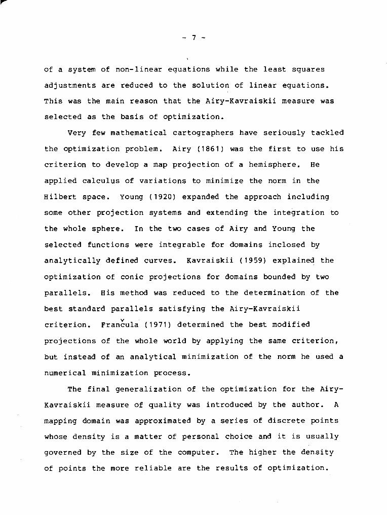
of a system of non-linear equations while the least squares
adjustments are reduced to the solution of linear equations.
This was the main reason that the Airy-Kavraiskii measure was
selected as the basis of optimization.
Very few mathematical cartographers have seriously tackled
the optimization problem. Airy ( 1 8 6 1 ) was the first to use his
criterion to develop a map projection of a hemisphere. He
applied calculus of variations to minimize the norm in the
Hilbert space. Young ( 1920 ) expanded the approach including
some other projection systems and extending the integration to
the whole sphere. In the two cases of Airy and Young the
selected functions were integrable for domains inclosed by
analytically defined curves. Kavraiskii ( 1959 ) explained the
optimization of conic projections for domains bounded by two
parallels. His method was reduced to the determination of the
best standard parallels satisfying the Airy-Kavraiskii
criterion. ~ranrula ( 1971) determined the best modified
projections of the whole world by applying the same criterion,
but instead of an analytical minimization of the norm he used a
numerical minimization process.
The final generalization of the optimization for the Airy-
Kavraiskii measure of quality was introduced by the author. A
mapping domain was approximated by a series of discrete points
whose density is a matter of personal choice and it is usually
governed by the size of the computer. The higher the density
of points the more reliable are the results of optimization.
I
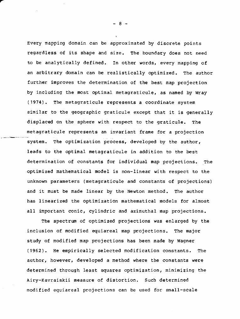
Every mapping domain can be approximated by discrete points
regardless of its shape and size. The boundary does not need
to be analytically defined. In other words, every mapping of
an arbitrary domain can be realistically optimized. The author
further improves the determination of the best map projection
by including the most optimal metagraticule, as named by Wray
(1974). The metagraticule represents a coordinate system
similar to the geographic graticule except that it is generally
displaced on the sphere with respect to the graticule. The
metagraticule represents an invariant frame for a projection *__- -
system. The optimization process, developed by the author,
leads to the optimal metagraticule in addition to the best
determination of constants for individual map projections. The
optimized mathematical model is non-linear with respect to the
unknown parameters (metagraticule and constants of projections)
and it must be made linear by the Newton method. The author
has linearized the optimization mathematical models for almost
all important conic, cylindric and azimuthal map projections.
The spectrum of optimized projections was enlarged by the
inclusion of modified equiareal map projections. The major
study of modified map projections has been made by Wagner
(1962). He empirically selected modification constants. The
author, however, developed a method where the constants were
determined through least squares optimization, minimizing the
Airy-Kavraiskii measure of distortion. Such determined
modified equiareal projections can be used for small-scale

mappings of a r b i t r a r y domains when t h e p r o p e r t y of e q u i v a l e n c y
is e s s e n t i a l t o u s e r s .
Conformal map p r o j e c t i o n s have g e n e r a l l y l i t t l e impor tance
f o r s m a l l - s c a l e g e o g r a p h i c t r a n s f o r m a t i o n . They a r e , however,
fundamenta l f o r l a r g e - s c a l e t o p o g r a p h i c maps. The a u t h o r
b e l i e v e s no o p t i m i z a t i o n of mappings is comple te w i t h o u t
Chebyshev' s p r o j e c t i o n s which a r e t h e b e s t conformal p r o j e c -
t i o n s (Meshcheryakov, 1969) . They a r e d e f i n e d a s p r o j e c t i o n s
i n which t h e changes of s c a l e a r e minimized. Chebyshev ' s
theorem ( B i e r n a c k i , 1965) s t a t e s t h a t t h e n e c e s s a r y and
s u f f i c i e n t c o n d i t i o n of t h e b e s t conformal p r o j e c t i o n is to
have a c o n s t a n t s c a l e f a c t o r a long t h e boundary c o n t o u r of t h e
domain. The Russ ian c a r t o g r a p h i c s choo l (Urmaev, 1953 ) has
so lved t h e problem of o b t a i n i n g t h e b e s t conformal p r o j e c t i o n s
f o r symmetric bounda r i e s . The a u t h o r showed i n t h e f i r s t p a r t
of t h e t h i r d c h a p t e r t h e sugges t ed s o l u t i o n s of Urmaev us ing
s e v e r a l methods (method of R i t z , method of f i n i t e d i f f e r e n c e s ,
and method of l e a s t s q u a r e s ) . The comple t ion of t h e de t e rmina -
t i o n of Chebyshev' s p r o j e c t i o n s f o r most g e n e r a l non-symmetric
domains was deve loped by t h e a u t h o r . He used a complex
polynomial a s a mapping a n a l y t i c f u n c t i o n and computed t h e
c o e f f i c i e n t s of t h e polynomial by t h e method of l e a s t s q u a r e s .
The r e s u l t a n t l i n e of c o n s t a n t s c a l e approximated c l o s e l y t h e
boundary c o n t o u r .
I
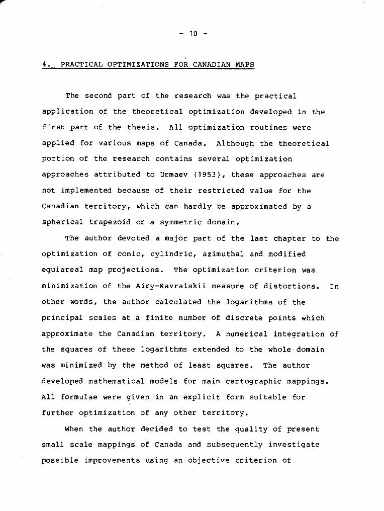
4. PRACTICAL OPTIMIZATIONS FOR CANADIAN MAPS
The second part of the research was the practical
application of the theoretical optimization developed in the
first part of the thesis. All optimization routines were
applied for various maps of Canada. Although the theoretical
portion of the research contains several optimization
approaches attributed to Urmaev (1 953 ) , these approaches are not implemented because of their restricted value for the
Canadian territory, which can hardly be approximated by a
spherical trapezoid or a symmetric domain.
The author devoted a major part of the last chapter to the
optimization of conic, cylindric, azimuthal and modified
equiareal map projections. The optimization criterion was
minimization of the Airy-Kavraiskii measure of distortions. In
other words, the author calculated the logarithms of the
principal scales at a finite number of discrete points which
approximate the Canadian territory. A numerical integration of
the squares of these logarithms extended to the whole domain
was minimized by the method of least squares. The author
developed mathematical models for main cartographic mappings.
All formulae were given in an explicit form suitable for
further optimization of any other territory.
When the author decided to test the quality of present
small scale mappings of Canada and subsequently investigate
possible improvements using an objective criterion of

I
deformations it was expected that the optimization would amount
to a small refinement to the present system resulting in a
marginally better graphical representation of Canada. The
numerical results of the research surpassed these hopes to an
unexpected amount. Every optimized map projection leads to a
much better mapping system than the presently used Lambert
Conformal Conic projection with standard parallels of 49' and
77'. In other words all projections optimized by the author
give better representation of Canada with less distortions than
the system in use. Particularly good results are obtained with - - - -- -- -
an oblique aspect of an equidistant conic projection whose
transformation formulae are very simple and therefore suitable
for providing the basis of a new small-scale map of Canada.
The overall deformations with this projection are 70 percent
smaller compared to the official projection.
The author believes that from theoretical point of view
this research for all practical purposes completes the opti-
mization of small-scale mapping. However, the determination of
better geodetic mapping (projections of the ellipsoid of
rotation onto a plane) remains to be tackled. This research
also indicated that more studies could be done in the integra-
tion of the fundamental differential equations of geographic
mappings.

I. GENERAL T H E O R Y OF CARTOGRAPHIC MAPPINGS
1. INTRODUCTION TO THEORY OF SURFACES
L e t us c o n s i d e r a s u r f a c e S and on it a c l o s e d domain
D. The s u r f a c e is d e f i n e d by a se t o f c u r v i l i n e a r p a r a -
metric c o o r d i n a t e s u i , where i = 1 , 2 . The p o s i t i o n v e c t o r
of t h e s u r f a c e is
The s u r f a c e is c a l l e d r e g u l a r i f f o r e v e r y p o i n t , wh ich
b e l o n g s t o t h e domain D t h e f o l l o w i n g c o n d i t i o n is s a t i s f i e d
where
ar = - and a u l
A p o i n t i n which t h e v e c t o r p r o d u c t of t h e two t a n g e n t
v e c t o r s ftl and 1: is e q u a l t o z e r o is c a l l e d a s i n g u l a r
p o i n t of t h e p a r a m e t r i z a t i o n ( u l , u 2 ) and i t is e x c l u d e d from
t h e domain D ( G o e t z , 1 9 7 0 ) .
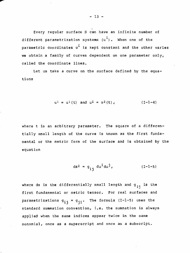
Every regular surface S can have an infinite number of
i different parametrization systems (u ) . When one of the
parametric coordinates ui is kept constant and the other varies
we obtain a family of curves dependent on one parameter only,
called the coordinate lines.
Let us take a curve on the surface defined by the equa-
tions
ul = ul(t) and u 2 = u2(t),
where t is an arbitrary parameter. The square of a differen-
tially small length of the curve is known as the first funda-
mental or the metric form of the surface and is obtained by the
equation
where ds is the differentially small length and gij is the
first fundamental or metric tensor. For real surfaces and
parametrizations gij - - gji0 The formula (1-1-5) uses the
standard summation convention, i.e. the summation is always
applied when the same indices appear twice in the same
monomial, once as a superscript and once as a subscript.

Thus , t h e e q u a t i o n (1-1-5) e x p l i c i t l y w r i t t e n becomes
For a g i v e n s u r f a c e and a s e l e c t e d p a r a m e t r i c c o o r d i n a t e
s y s t e m w e o b t a i n a metric t e n s o r
w i t h componen t s
The i n d i v i d u a l components of t h e m e t r i c t e n s o r a r e o b t a i n e d by
t h e s c a l a r p r o d u c t s of t h e c o r r e s p o n d i n g t a n g e n t v e c t o r s +, and r2.

The d i s c r i m i n a n t of t h e f i r s t f u n d a m e n t a l form, d e n o t e d by
i A s u r f a c e is r e g u l a r f o r a c h o s e n p a r a m e t r i z a t i o n ( u )
when
The t a n g e n t v e c t o r a t o t h e c u r v e (1-1-4) c a n be d e f i n e d a s a
l i n e a r c o m b i n a t i o n of t h e t a n g e n t v e c t o r s t o p a r a m e t r i c c u r v e s
i where a a r e t h e components of a w i t h r e s p e c t t o t h e coor -
d i n a t e s y s t e m ( u l ) . I f w e t a k e a n o t h e r c u r v e which i n t e r s e c t s
t h e f i r s t and d e n o t e its t a n g e n t v e c t o r a t t h e common p o i n t o f
t h e two c u r v e s by b , t h e n t h e a n g l e u be tween t h e two c u r v e s
is o b t a i n e d from t h e s c a l a r p r o d u c t of t h e t a n g e n t v e c t o r s
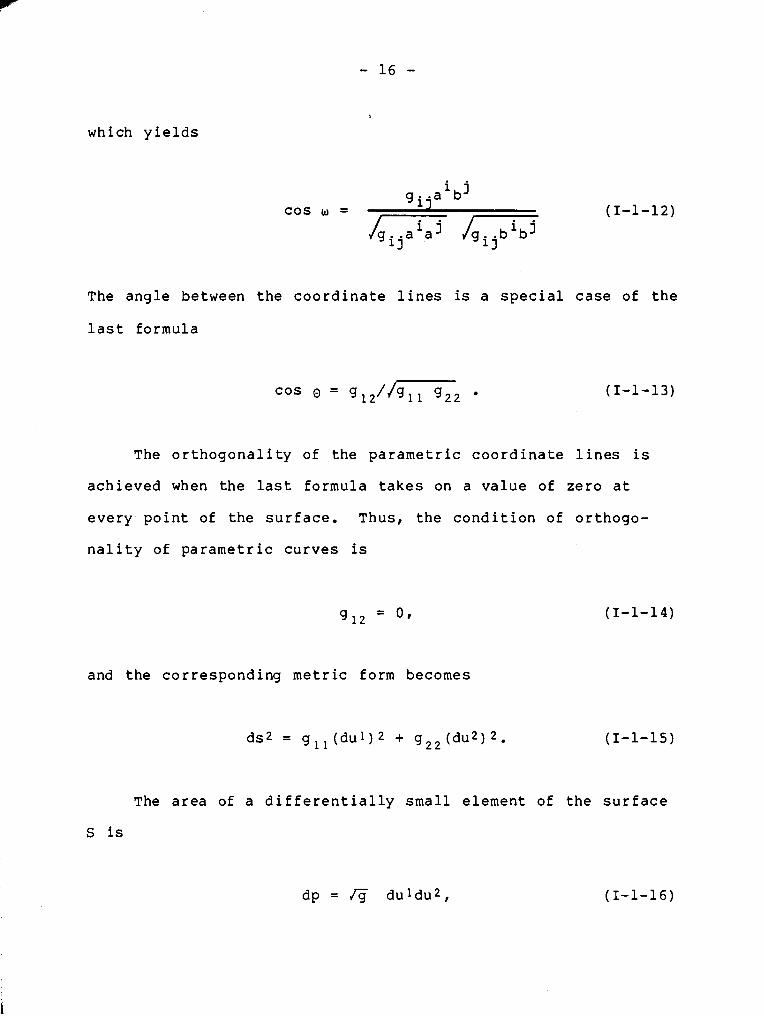
which yields
-IJ COS W = (1-1-12)
The angle between the coordinate lines is a special case of the
last formula
cos 0 = 912'4911 922
The orthogonality of the parametric coordinate lines is
achieved when the last formula takes on a value of zero at
every point of the surface. Thus, the condition of orthogo-
nality of parametric curves is
and the corresponding metric form becomes
The area of a differentially small element of the surface

,
and its i n t e g r a t i o n f o r t h e whole domain
The e l emen t s of s u r f a c e s ( a d i f f e r e n t i a l l y s m a l l d i s t a n c e ,
d s , an a n g l e between two c u r v e s of t h e s u r f a c e , w , and t h e
a r e a of t h e domain, A ) a r e known a s t h e i n t r i n s i c e l emen t s of D
t h e s u r f a c e s i n c e t h e y a r e i n v a r i a n t no m a t t e r which parame-
t r i z a t i o n is s e l e c t e d . I n o t h e r words, t h e c o o r d i n a t e s can be
changed bu t t h e v a l u e s of i n t r i n s i c e l emen t s remain u n a l t e r e d .
To s i m p l i f y t h e deve lopments of formulae i n c e r t a i n t y p e s
of mappings, w e can make a s p e c i f i c p a r a m e t r i z a t i o n of t h e
s u r f a c e which l e a d s t o a p a r t i c u l a r t ype of t h e f i r s t funda-
menta l form.
For example, i f g l = 1 and g12 = 0 we o b t a i n t h e , so-
c a l l e d , s emigeodes i c c o o r d i n a t e s w i t h t h e f i r s t fundamenta l
form
When g l l = g 2 2 and g 1 2 = 0 t h e r e s u l t i n g c o o r d i n a t e s a r e
c a l l e d i s o m e t r i c i n geodesy and i s o t h e r m i c i n mathematics . The
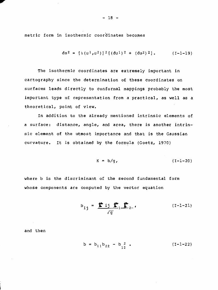
m e t r i c form i n i s o t h e r m i c c o o r d i n a t e s becomes
The i s o t h e r m i c c o o r d i n a t e s a r e ex t r eme ly impor t an t i n
c a r t o g r a p h y s i n c e t h e d e t e r m i n a t i o n of t h e s e c o o r d i n a t e s on
s u r f a c e s l e a d s d i r e c t l y t o conformal mappings p robab ly t h e most
i m p o r t a n t t ype of r e p r e s e n t a t i o n from a p r a c t i c a l , a s w e l l a s a
t h e o r e t i c a l , p o i n t of view.
I n a d d i t i o n t o t h e a l r e a d y mentioned i n t r i n s i c e lements of
a s u r f a c e : d i s t a n c e , a n g l e , and a r e a , t h e r e is a n o t h e r i n t r i n -
s i c e lement of t h e utmost impor tance and t h a t is t h e Gauss ian
c u r v a t u r e . I t is o b t a i n e d by t h e formula (Goetz , 1970)
where b is t h e d i s c r i m i n a n t of t h e second fundamental form
whose components a r e computed by t h e v e c t o r e q u a t i o n
and t h e n

Mathematical c a r t o g r a p h y g e n e r a l l y d e a l s wi th t h r e e
d i f f e r e n t s u r f a c e s : p l a n e , s p h e r e and s p h e r o i d .
The p l a n e is a s u r f a c e whose Gauss ian c u r v a t u r e is e q u a l
t o zero . I f we adop t an o r t h o g o n a l C a r t e s i a n c o o r d i n a t e system
i ( x ) t h e f i r s t fundamental form on t h e p l a n e becomes
ds2 = (dx 1 ) 2 + ( d ~ 2 ) 2 . (1-1-23)
The s p h e r e and t h e s p h e r o i d , on t h e o t h e r hand, belong t o
s u r f a c e of r o t a t i o n , which a r e d e f i n e d by t h e r o t a t i o n of a
p l a n a r cu rve abou t an a x i s . The a x i s of r o t a t i o n l i e s i n t h e
p l a n e of t h e cu rve . Var ious p o s i t i o n s of t h e r o t a t i n g cu rve
a r e c a l l e d m e r i d i a n s of t h e s u r f a c e .
A s p h e r e is a s p e c i a l c a s e of a s u r f a c e of r o t a t i o n
g e n e r a t e d by t h e r o t a t i o n of a s e m i c i r c l e of r a d i u s R, whose
v e c t o r is
4 4
w i t h b ,J , being m u t u a l l y o r t h o g o n a l v e c t o r s .
The f i r s t fundamental form on t h e s p h e r e is

and t h e Gauss i an c u r v a t u r e becomes
s i n c e
A s p h e r o i d is o b t a i n e d by t h e r o t a t i o n of a m e r i d i a n
e l l i p s e about i ts semi-minor a x i s . Its s u r f a c e is used t o
approximate t h e a c t u a l s u r f a c e of t h e e a r t h f o r g e o d e t i c
p o s i t i o n i n g and, s u b s e q u e n t l y , f o r g e o d e t i c mappings, b u t t h e s e
a r e o u t s i d e t h e scope of t h i s work. Thus it s u f f i c e s t o g i v e
t h e fundamental formula of a s p h e r o i d
where N is t h e maximal r a d i u s of c u r v a t u r e a t a p o i n t ( u l , u 2 )
o b t a i n e d by t h e e x p r e s s i o n
a is t h e semi-major a x i s of t h e mer id i an e l l i p s e and e2 is t h e
s q u a r e of t h e e c c e n t r i c i t y

I
and b is the semi-minor axis of the meridian ellipse.
The components of the fundamental metric tensor are
with M being the radius of curvature of the meridian ellipse
Thus, the first fundamental form is
and the Gaussian curvature is
K = l/MN.
2. CARTOGRAPHIC MAPPINGS
Let us consider two regular surfaces, S and P, and on the
first surface S, a closed domain D. Both surfaces are defined
by a corresponding set of curvilinear parametric coordinates:
i i (u ) on St and (x ) on P, for i = 1,2.
Then the relationship
x1 = x1(u11u2) and x2 = x2(ultu2) (1-2-1)

defined in the domain, DES, establishes a connection between
points of the first surface A(ul,u2) ED and points of the
second surface B(xl,x2), which belong to some domain A. In
other words, the domain D of the first surface is transformed
into the domain, A of the second surface, or the domain D is
projected onto the second surface in the domain A. To make
projections or mappings meaningful in practice, the class of
transformation functions (1-2-1) is restricted to those
functions which are unique, twice differentiable and continuous
up to the second derivative, finite, and where in all points
the Jacobian determinant must be different from zero, i.e.
Such an established one-to-one correspondence between the
points of the two domains, which is continuous in both direc-
tions, is called a homeomorphism.
The first surface is commonly called the original surface
and the second surface is then the projection surface.
Under homeomorphism, however, the transformation direction is
reversible and the mapping can be also performed from the
second onto the first surface
u1 = u1 (XI ,x2) and u2 = u2 (XI ,x2) . (1-2-3)
Commonly, the first set of formulae (1-2-1) is known as
the direct or forward solution, while the second set (1-2-3)

r e p r e s e n t s t h e i n v e r s e s o l u t i o n of t h e mapping problem.
Ca r tog raphy assumes t h e e a r t h t o be a s p h e r e of r a d i u s R
and t h e p r o j e c t i o n s u r f a c e a p l a n e . Thus, t h e s u b j e c t of math-
e m a t i c a l c a r t o g r a p h y f o r g e o g r a p h e r s is main ly r e s t r i c t e d t o
v a r i o u s t y p e s of t r a n s f o r m a t i o n s of t h e s p h e r e o n t o t h e p l a n e .
D i f f e r e n t i a l geometry (Goetz , 1970; Taschne r , 1977) shows
t h a t a mutual p r o j e c t i o n of two s u r f a c e s is e x p l i c i t l y d e f i n e d
by t h e metrics of t h e s u r f a c e s . The metric t e n s o r depends upon
a s u r f a c e and a s e l e c t e d p a r a m e t r i z a t i o n , a s was s t a t e d i n
(1-1-7) . The fundamenta l set of p a r a m e t r i c c u r v i l i n e a r c o o r d i -
n a t e s on t h e s p h e r e c o n s i s t s of t h e g e o g r a p h i c l a t i t u d e , 4 , and
t h e g e o g r a p h i c l o n g i t u d e A. The l a t i t u d e of a p o i n t is t h e
a n g l e between t h e r a d i a l l i n e th rough t h e p o i n t and t h e equa-
t o r i a l p l a n e . I n i t s magni tude, t h e l a t i t u d e can be between 0'
and 90' w i t h , c o n v e n t i o n a l l y , t h e p o s i t i v e a l g e b r a i c s i g n f o r
t h e l a t i t u d e s of t h e n o r t h e r n hemisphere and t h e n e g a t i v e f o r
t h e s o u t h e r n hemisphere . The l o n g i t u d e of a p o i n t is t h e a n g l e
reckoned from t h e i n i t i a l m e r i d i a n p l a n e , a l s o c a l l e d t h e
Greenwich m e r i d i a n , e a s t w a r d l y o r wes tward ly t o t h e m e r i d i a n o f
t h e p o i n t i n q u e s t i o n . I n i t s magni tude , t h e l o n g i t u d e s can be
between 0' and 180'. Eas tward ly measured l o n g i t u d e s a r e con-
v e n t i o n a l l y t aken t o be p o s i t i v e and wes t e rn l o n g i t u d e s ,
n e g a t i v e . The i n i t i a l o r c e n t r a l m e r i d i a n of a mapped t e r r i -
t o r y seldom c o i n c i d e s w i t h t h e i n i t i a l m e r i d i a n of t h e geo-
g r a p h i c system, t h e Greenwich m e r i d i a n . T h e r e f o r e , c a r t o g -
r a p h e r s , i n s t e a d of u s ing l o n g i t u d e s use t h e d i f f e r e n c e s of
l o n g i t u d e s between t h e l o n g i t u d e of a p o i n t , A , and t h e

, l o n g i t u d e of t h e s e l e c t e d c e n t r a l m e r i d i a n , X o '
Thus, i n c a r t o g r a p h y each p o i n t on t h e s p h e r e is d e f i n e d
by t h e l a t i t u d e , 0 , and t h e d i f f e r e n c e i n l o n g i t u d e , 1. The
c o o r d i n a t e l i n e s c o n s i s t of m e r i d i a n s , l i n e s of c o n s t a n t 1, and
p a r a l l e l s , l i n e s of c o n s t a n t 4.
The p r o j e c t i o n s u r f a c e is a p l a n e wi th e i t h e r an or thog-
o n a l C a r t e s i a n c o o r d i n a t e system ( x , y ) o r a p o l a r c o o r d i n a t e
sys tem (y ,Q). S i n c e t h e change from r e c t a n g u l a r i n t o p o l a r
c o o r d i n a t e s and v i c e v e r s a is accompl i shed by s i m p l e t r a n s -
f o r m a t i o n formulae , i t w i l l be assumed, a t l e a s t i n t h e
p r e l i m i n a r y c o n s i d e r a t i o n s , t h a t p o i n t s of t h e mapping p l a n e
a r e d e f i n e d by t h e i r r e c t a n g u l a r C a r t e s i a n c o o r d i n a t e s .
Thus, a mapping system e s t a b l i s h e s a law of t r a n s f o r m a t i o n
of c u r v i l i n e a r s p h e r i c a l c o o r d i n a t e s ( + ,1) i n t o t h e p l a n e
c o o r d i n a t e s ( x , y ) . To each p o i n t of t h e s p h e r e t h e t r a n s f o r -
mat ion f u n c t i o n s a s s i g n a unique p o i n t on t h e p l ane . The
g e n e r a l t r a n s f o r m a t i o n formulae f o r t h e d i r e c t and i n v e r s e
compu ta t ions (1-2-1) and (1-2-3) can be t r a n s c r i b e d f o r c a r -
t o g r a p h i c mappings i n t o t h e fo l lowing p a r a m e t r i c e q u a t i o n s

and
where the first set of equations defines the direct mapping and
the second set the inverse mapping. The transformation func-
tions must satisfy the same conditions as the general formulae
(1-2-1) of continuity, differentiability up to the second
derivative, uniqueness, finiteness and the Jacobian determinant
must differ from zero, a (x,y)/a (+,l) 1: 0. In other words, the
mapping functions must be homeomorphic.
The fundamental metric on the sphere, according to the
formula (1-1-15) Is
ds2 = l?2(d$,2 + C O S ~ + d12),
and that on the plane
where dS is a differentially small linear element on the plane,
obtained as an image of the corresponding linear element ds on
the sphere, and the image is realized by the transformation
functions (1-2-5) . Since the rectangular coordinates (x,y) are
functions of spherical coordinates (+,1), the differentials in
the last formula (1-2-8) are
dx = x d+ + xldl and dy = y+d+ + yldl. $
(1-2-9)

, When the differentials (1-2-9) are substituted into the
equation (1-2-8) we obtain the well known expression for the
square of a differentially small distance in the plane as a
SPHERE PLANE ,
Figure 1-2-1 Coordinate systems in cartographic mappings
function of spherical coordinates
d ~ 2 = g l l d $ 2 + 2g12d$dl + g2,d12,

where
SPHERE :
e
PLANE:
7
F i g u r e 1-2-2 D i f f e r e n t i a l l y s m a l l s u r f a c e e l e m e n t o f t h e s p h e r e
and i ts p r o j e c t i o n i n t h e p l a n e
The a z i m u t h of a d i f f e r e n t i a l l y s m a l l l i n e segment d s on
t h e s p h e r e is d e f i n e d a s t h e a n g l e r eckoned c l o c k w i s e from t h e
p o s i t i v e d i r e c t i o n of t h e m e r i d i a n t o t h e segment and is

, d e n o t e d by a . I ts t a n g e n t f u n c t i o n is o b t a i n e d from t h e s m a l l
r i g h t a n g l e t r i a n g l e ABC on t h e f i g u r e 1-2-2, namely
t a n a = c o s $ d l / d $ . (1-2-12)
The g r i d b e a r i n g , 3 , is t h e a n g l e on t h e p r o j e c t i o n p l a n e
between t h e d i r e c t i o n of t h e y - a x i s of t h e p l a n e c o o r d i n a t e
s y s t e m , measured c l o c k w i s e , and t h e p r o j e c t i o n of t h e a r c
segment dS, namely
From t h e above e q u a t i o n one c a n a l s o d e t e r m i n e t h e b e a r i n g
o f t h e p r o j e c t i o n of m e r i d i a n (1 = c o n s t . , d l = 0 ) and p a r a l l e l
( $ = c o n s t . , d$ = 0 )
t a n ) = x m / y m and t a n x = xl/yl (1-2-14)
The p r o j e c t i o n of t h e a z i m u t h a , d e n o t e d by a ' is t h e n

Thus
Substituting the values for tan f3 and tan $I from (1-2-14)
respectively and rearranging the terms, we have
cot a' = ,,/m 2 + g12/fi, dl
where
The angle between the projections of parametric curves is
computed by the formula (1-1-13)
The sine function of angle e is then

A d i f f e r e n t i a l l y s m a l l a r e a on t h e s p h e r e l i m i t e d by two
c l o s e m e r i d i a n s and p a r a l l e l s is
dp = ~2 cos + d+ d l , (1-2-21)
and its p r o j e c t i o n on t h e p l a n e becomes
dP = 4q-d$ d l . ( 1-2-22 )
Thus w e have d e f i n e d a l l t h e i m p o r t a n t i n t r i n s i c e l e m e n t s
__- - o f t h e sphe re : a d i f f e r e n t i a l l y sma l l d i s t a n c e , d s , and i ts
az imuth , a , a d i f f e r e n t i a l l y sma l l a r e a , dp, and t h e corre-
sponding p r o j e c t i o n s on t h e p l a n e dS, a', dP, a s f u n c t i o n s of
t h e d i f f e r e n t i a l s d$ and d l . The a p p r o p r i a t e l o g i c a l compar-
i s o n of t h e i n t r i n s i c e l emen t s p r o v i d e s us w i t h measures of
q u a l i t y f o r v a r i o u s p r o j e c t i o n sys tems .
3 . THEORY OF DISTORTIONS
D i f f e r e n t i a l geometry (Goe tz , 1970) shows t h a t an isomet-
r i c mapping of two s u r f a c e s , a mapping where a l l c o r r e s p o n d i n g
d i s t a n c e s on both s u r f a c e s remain i d e n t i c a l , can be o b t a i n e d i f
and o n l y i f t h e Gauss i an c u r v a t u r e s of both s u r f a c e s a r e
i d e n t i c a l . S i n c e t h e Gauss i an c u r v a t u r e of a s p h e r e is e q u a l
t o t h e i n v e r s e of t h e s q u a r e of t h e r a d i u s , and t h a t of t h e
p l a n e is equa l t o ze ro , it is i m p o s s i b l e t o d e r i v e t r a n s f o r -
ma t ion formulae which, g e n e r a l l y , w i l l no t a l t e r d i s t a n c e s .

In other words, the mapping prbcess will always cause a certain
deformation of the original intrinsic elements. Although some
of the intrinsic elements may be preserved in the mapping pro-
cess, the complete identity of the original surface elements
and their projected counterparts can never be achieved in car-
tographic projections.
One of the main tasks of mathematical cartography is to
determine a projection of a mapped territory in such a way that
the resulting deformations of the original intrinsic elements
are objectively minimized. Thus, distances, angles and areas
will generally be changed in the transformation process.
However, the changes of projected distances, angles and areas,
and in particular the variations of these changes must be made
as small as possible by the appropriate choice of transfor-
mation formulae. Distortions of surfaces in cartographic
mappings are infinitely versatile, but, considered locally, the
variations of the same distortions around an arbitrary point of
a projected domain are governed by the general laws valid for
all analytically defined projection systems. These laws are
the subject of the theory of distortions. They were developed
by a French mathematician and cartographer, M. Tissot
(1824-1897) in 1859, with their final version being published
in 1881 in Tissot's 'Memoirs'.
The theory of distortion is relatively well covered in
textbooks of mathematical cartography, e.g. (Biernacky, 1965),
(Fiala, 1957), (Kavraisky, 1959), (Richardus, Adler, 1972) and
many others. In the English language it still remains to be

t r e a t e d r i g o r o u s l y ; however, t h e r e is no need t o r e d e v e l o p a l l
t h e formulae of t h e t h e o r y of d i s t o r t i o n s . I t w i l l s u f f i c e t o
l i s t and e x p l a i n them, s i n c e they a r e used l a t e r when e v a l u a t e d
n u m e r i c a l l y .
The comparison of a d i f f e r e n t i a l l y s m a l l d i s t a n c e on t h e
s p h e r e and its p r o j e c t i o n on t h e p l a n e is made by t h e s c a l e
f a c t o r , k .
where ds is t h e s p h e r i c a l d i s t a n c e and dS is its p l a n a r
c o u n t e r p a r t . The i d e a l v a l u e of t h e s c a l e is u n i t y , i n which
c a s e , a d i s t a n c e on t h e s p h e r e and its p r o j e c t i o n on t h e p l a n e
a r e i d e n t i c a l . The d i s t o r t i o n of d i s t a n c e s is then d e f i n e d by
t h e e q u a t i o n
From t h e fundamental d e f i n i t i o n of t h e s c a l e (1-3-1) and
by us ing t h e e x p r e s s i o n s (1-2-7) and (1-2-8) we have t h e v a l u e
f o r t h e s q u a r e of t h e s c a l e

which can e a s i l y be t r ans fo rmed i n t o
c o s 2 ~ + .A s i n 2a + (1-3-3) R c o s 4
where a is t h e azimuth of t h e o r i g i n a l d i s t a n c e d s on t h e
s p h e r e and g i j a r e t h e e l emen t s of t h e m e t r i c t e n s o r . I t is
obv ious from t h e l a s t formula t h a t t h e s c a l e i n g e n e r a l depends
on t h e p o s i t i o n of a p o i n t ( g i j ) and t h e d i r e c t i o n of t h e l i n e
segment a t t h e p o i n t ( a ) , i . e .
- - k = k ( g i j , a ) . (1-3-4)
The s c a l e s a long t h e p a r a m e t r i c c o o r d i n a t e l i n e s ,
m e r i d i a n s and p a r a l l e l s a r e d e r i v e d d i r e c t l y from t h e e q u a t i o n
(1-2-25) knowing t h a t f o r m e r i d i a n s a = 0 , and f o r p a r a l l e l s
a = sr/2, t h u s
and
n = G 2 / R c o s 6 , (1-3-6)
where m is t h e s c a l e a long m e r i d i a n s and n a long p a r a l l e l s .

The e q u a t i o n (1-3-3) can a l s o be exp res sed i n terms of m,n
and t h e p a r a m e t r i c a n g l e 8, i . e .
k2 = m2 C O S ~ ~ + mn c o s 8 s i n 2a + n 2 s i n 2 a . (1-3-7)
The extreme v a l u e s of t h e s c a l e a r e o b t a i n e d from t h e
e q u a t i o n d ( k * ) / d a = 0 which y i e l d s
t a n 2ao = 29 l 2 (20s 4 I (1-3-8) g l l c0s2$ -
where a. and a. + n/2 i n d i c a t e two a n g l e s t h a t s a t i s f y t h e
above t r i g o n o m e t r i c e q u a t i o n and r e p r e s e n t t h e d i r e c t i o n s of
t h e extreme s c a l e changes . These two o r t h o g o n a l d i r e c t i o n s a r e
c a l l e d t h e p r i n c i p a l d i r e c t i o n s and t h e i r main c h a r a c t e r i s t i c
is t h a t t hey remain o r t h o g o n a l on t h e p r o j e c t i o n p l a n e a s w e l l .
The d e f i n i t i o n and meaning of t h e p r i n c i p a l d i r e c t i o n s a r e
fo rmula t ed by T i s s o t i n h i s 'Memoirs1 ( ~ a v r a i s k i i , 1959) i n t h e
f i r s t theorem of mappings.
. . . In eve ry non-conf ormal r e p r e s e n t a t i o n of a r e g u l a r s u r f a c e o n t o a n o t h e r t h e r e is one and o n l y one p a i r of co r r e spond ing o r t h o g o n a l d i r e c t i o n s which a r e t h e p r i n c i p a l d i r e c t i o n s and they r e p r e s e n t t h e d i r e c t i o n s of t h e ex t reme s c a l e s . . ..
The d i s t o r t i o n of a r e a s v is t h e d i f f e r e n c e between u n i t y P
and t h e s c a l e of a r e a p

where p is defined as the ratio of a differentially small area
on the plane and its original value on the sphere, namely
Substituting in the above formula the expressions for
areas dp, dP (1-2-21) and (1-2-22) we have
p = mn sin 8 . (1-3-12)
The projection of the parametric angle, 8, is computed
either by the equations (1-2-19) and (1-2-20) or
tan 8 = m/gl2. (1-3-13)
The deformation of the parametric angle is defined by
E: = n/2 - 8 ,
and its tangent function is
tan E = - g 12/fi

I
The a n g u l a r d e f o r m a t i o n w is d e f i n e d a s t h e d i f f e r e n c e
between an azimuth a and its p r o j e c t i o n a ' , i . e .
I ts numer ica l v a l u e can be o b t a i n e d from t h e e x p r e s s i o n
t a n w = 411 c o s $ + g l t a n a - fi , (1-3-17)
g l l c o s $ c o t a + g12 + fl t a n a
bu t t h e same formula w i l l be g i v e n l a t e r i n a form more -- -
s u i t a b l e f o r numer i ca l compu ta t ions .
A t t h e end of t h i s s e c t i o n it must be emphasized t h a t a
g r e a t m a j o r i t y of t h e formulae from t h e t h e o r y of d i s t o r t i o n s
were a l r e a d y known t o L. Eu le r b u t t h e i r comple te and f i n a l
form was e l a b o r a t e d o n l y a c e n t u r y ago by T i s s o t . However, f o r
r ea sons unknown t o t h e a u t h o r , c a r t o g r a p h e r s i n E n g l i s h
speak ing c o u n t r i e s have been r e l u c t a n t e i t h e r t o adop t them o r
t o deve lop them f u r t h e r . Only i n t h e l a s t decade have w e been
e x p e r i e n c i n g a c e r t a i n i n t e r e s t i n ma thema t i ca l problems of
c a r t o g r a p h y (Mi lno r , 1969) .
4 . I N D I C A T R I X OF TISSOT
I n h i s s t u d y of g e n e r a l c a r t o g r a p h i c t r a n s f o r m a t i o n s
T i s s o t i n t roduced an e l l i p s e of d i s t o r t i o n o r t h e i n d i c a t r i x of
p r o j e c t i o n , which found a p a r t i c u l a r l y i m p o r t a n t p l a c e i n

mathematical cartography. iss sot's indicatrix, as a geometric characteristic of a mapping system, explained the fundamental
questions of deformations of intrinsic elements and gave the
distortions a more natural character and a more readily appli-
cable visible form. The indicatrix of Tissot, with all its
elements defined, completely describes the cartographic trans-
formation system, or in other words, every measure of distor-
tion can be expressed as a function of parameters of the
indicatrix of Tissot (Biernacki, 1965) . The ellipse of distortion at a point of a projected domain
is obtained by the transformation of a differentially small
circle of unit radius from the original surface of the sphere
onto the projection plane. The circle is generally transformed
into an ellipse whose semi-axes are projected in the principal
directions and in their magnitude they are equal to the extreme
scale factors. The semi-major axis a is the maximal scale at
the point PI and the semi-minor axis b is the minimal scale.
The most suitable coordinate systems are the orthogonal local
systems with the principal directions on both surfaces as the
coordinate axes ( 5 , q ) on the sphere and (x,y) on the plane.
The semi-axes of the indicatrix are computed from known
scales along the parametric curves, m and n, and the projected
parametric angle, 8.
1 1 a = - (A + B) and b = - (A - B) (1-4-1) 2 2

where
A 2 = m 2 + n2 + 2mn s i n 8 , (1-4-2)
B* = m 2 + n2 - 2mn sin 0 .
SPHERE: PLANE :
M A P P I N G
F i g u r e 1 - 4 - 1 U n i t c i r c l e and t h e i n d i c a t r i x of T i s s o t

1
The orientation angle of the meridian with respect to the
first principal direction, 6, is
and its projection on the plane, B ' , is
tan 6' = b tan 6. a
If we'take an arbitrary direction, 6, with respect to the
first principal direction, then the scale factor in its
direction, k can be expressed in terms of the extreme scales
and the direction angle, 6.
The angular distortion, defined again as the difference
between the original direction, 6, and its projection, 6', is
and

where t h e p r o j e c t i o n a n g l e , 6 ' , is computed by t h e formula
(1-4-4).
The maximal a n g u l a r d i s t o r t i o n , w o , is
, a - b s i n w 0 - - , a + b
and it o c c u r s when s i n ( 6 + 6 ' ) = 1, o r 6 + 6 ' = n/2.
The d i r e c t i o n , 6 0 , i n which t h e maximal a n g u l a r d i s t o r t i o n
t a k e s p l a c e is computed from t h e r e l a t i o n s h i p
and its p r o j e c t i o n
The s c a l e of a r e a s , p, can a l s o be exp res sed i n terms of
t h e pa rame te r s of t h e i n d i c a t r i x of T i s s o t by
p = ab.

I
When the fundamental equations of a geographic mapping
(1-2-5) are given, various quantities can be computed that
fully characterize distortions. These quantities then specify
the properties of the transformation system. They are: the
scale factor k t the scales along parametric curves, m and n,
the projection of the parametric angle, 9, the extreme scales,
a and b, the bearing of the meridian, I#, and that of the par-
allel, x, the scale of areas, p, and many others. Since these
quantities completely describe a projection, they are called
the characteristics of mapping. Each of the characteristics
can be defined as a function of eight variables
where Xi is an arbitrary characteristic. From the totality of
all characteristics we can select different vectors of four
independent characteristics and then all others can be
expressed in terms of the chosen basic vector. As a basic
vector we may take, for example, (a, b a I # , (m, n, I # x) , (m, n, I#, e ) , etc. The independence of a set of four charac-
teristics can be determined by the analysis of the corre-
sponding formulae. A more appropriate and a more rigorous
approach is to prove that the set of four independent charac-
teristics satisfies the following inequality
I
If the Jacobian (1-4-13) is nonsingular, and thus the four
characteristics are independent, we can determine a unique set
of transformation formulae (1-2-5) from the differentials
5. FUNDAMENTAL DIFFERENTIAL EQUATIONS
As shown in the preceding section, any combination of four
independent characteristics of map projections, Xi
(i = 1, 2, 3, 4) may serve as the basis of the vector space of
all deformation parameters. Therefore, the specification of
the four basic characteristics as functions of + and 1 at every point of the mapping domain fully determines the mapping
system. In other words, it must be theoretically possible to
derive the final transformation functions x = x(+,l) and
y = y(+,l) directly from a specified distribution of distor-
tions defined by the basis vector.
Let us now take two suggestions for the basis vectors made
by Russian cartographers G.A. Meshcheryakov and N.A. Urmaev.
The former (Meshcheryakov, 1968) recommended the basis vector
(m, n, 8, J I ) and the latter (Urmaev, 1953) (m, n, E , p) . We
shall develop both systems in order to obtain the fundamental
differential equations of map projections with respect to both
bases.
Meshcheryakov's suggestion of (m, n, 0 , $) uses the known

, expressions for scales along parametric curves (1 -3 -5 ) and
( I - 3 - 6 ) , and the bearings of the projections of parametric
curves, whose tangent functions were given by the formulae
( I - 2 - 1 4 ) , bearing in mind that the parametric angle e is
defined by the equation
When the elements of the metric tensor gij are substituted
into the equations (1-3-5) and (1 -3 -6 ) and the equations are
squared we have
The formulae (1-2-14) can be rewritten in the form
and 4l = y$ tan + y$ cP
= x cot $
(1-5-3)
x = yl tan x , 1 y1 = X1 cot x.
When the last results are substituted into the equations
(1 -5 -2 ) and employing the trigonometric identities
1 + tan2$ = sec2q , 1 + cot29 = csc2q

we obtain
Y4 = Rm cos $ , yl = R cos 4 n cos ,
and
x = Rm sin ) , xl = R cos 4 n sin . 4
The integration of equations (1-5-4) leads to the
transformation expressions (1-2-5) , providing the conditions of integrability are satisfied, namely
With the introduction of new abbreviations
m* = Rm and n* = Rn cos 4
the equation (1-5-4) becomes
Y4 = m* cos ) , yl = n* cos ,
X = m* sin ) , x = n* sin . 4 1

The c o n d i t i o n s of i n t e g r a b i l i t y (1-5-5) a r e t h e n
m* s i n y + m* c o s y y1 = n* s i n x + n* c o s x , 1 0 0
(1-5-8)
m* c o s IJJ - m* s i n IJJ I J J ~ = n* c o s x - n* s i n x x . 1 4 0
From t h e d e f i n i t i o n of p a r a m e t r i c a n g l e , 8 , (1-5-1) we
h a v e t h a t
x = 8 + l ; ) ,
and s u b s t i t u t e d i n t o e q u a t i o n s (1-5-8) w e o b t a i n
s i n $(m* - n* c o s 8 + n* s i n 8 IJJ + n* s i n 8 8 ) = 1 4 0 4
= - c o s +(m* yl - n* s i n 8 - n* c o s 8 y - n* c o s 8 8 ) , 4 4 4
and
c o s $(m* - n* c o s 8 + n* s i n 8 y + n* s i n 8 8 ) = 1 0 0 4
= s i n $(m* - n* s i n 8 - n* c o s 8 IJJ - n* c o s 8 8 ) , 0 4 4
o r s i m p l i f i e d
n s i n y = - u cos + ,
a Cos + = w s i n $ ,

where
and
u = m* - n* sin 8 - n* cos 8 JI - n* cos 8 8 . 0 0 0
The equations (1-5-10) then can be satisfied only if the
expressions Q and u are equal to zero, namely
m* - n* cos 8 + n* s i n e JI + n* sin 8 8 = 0, 1 0 0 0
1 (1-5-12) m*$l - n* sin 8 - n* cos 8 I$ - n* cos 8 8 = 0. 0 0 0
The system of partial differential equations (1-5-12) may
be called the fundamental system of differential equations of
map projections, since the system must be satisfied at every
point of the mapping domain. The system involves four charac-
teristics m,n,g,$ and their partial derivatives of the first
order with respect to the parametric coordinates ( 1 ) The
equations are quasilinear with respect to any combination of
two characteristics from the basis vector m,n,B,qt. The system
of two equations connects four functions and, thus, it is
undetermined. For practical applications of the fundamental
system we must predefine the values of two characteristics, or

e s t a b l i s h two r e l a t i o n s betwebn them a t eve ry p o i n t of t h e
mapping domain. Only then is t h e r e a t h e o r e t i c a l p o s s i b i l i t y
of i n t e g r a t i o n of t h e e q u a t i o n s (1-5-12).
The b a s i s v e c t o r of Urmaev ( m , n , ~ ,p) r e q u i r e s t h e equa-
t i o n s (1-5-2)
I n a d d i t i o n t o them, t h e t a n g e n t f u n c t i o n of t h e
d e f o r m a t i o n of p a r a m e t r i c a n g l e , E , is g i v e n by t h e e q u a t i o n
(1-5-15)
t a n E = - 9 1 2 . , rn
and from (1-3-11)
a = ~2 c o s 4 p.
Thus
t a n E = - 1
R 2 cos 4 p 912 '
o r f i n a l l y
t a n = - - -I- R Z c o s , p ( x , x 1 + Y , Y ~ ) *

The s e l e c t e d t r a n s f o r m a t i o n f u n c t i o n s x = x ( + , l ) and
y = y ( + , l ) must s a t i s f y a t eve ry p o i n t of t h e domain t h e
e q u a t i o n s (1-5-13) and (1-5-14). The e s t a b l i s h m e n t of new
c o o r d i n a t e sys tems r e q u i r e s t h e i n t e g r a t i o n of t h e same t h r e e
e q u a t i o n s . However much we may wish t o c a r r y o u t t h e op t imi -
z a t i o n p r o c e s s and, t h u s , reduce d i s t o r t i o n s t o any d e s i r a b l e
l e v e l we cannot go too f a r s i n c e t h e r e l a t i o n s between d i s t o r -
t i o n e l emen t s (1-5-13) and (1-5-14) must a lways e x i s t .
Without a l o s s of g e n e r a l i t y , Urmaev assumed t h e u n i t
r a d i u s of t h e e a r t h and h a s r e p l a c e d i n (Urmaev, 1953) t h e
e q u a t i o n s (1-5-13) and (1-5-14) by f o u r e x p r e s s i o n s
x = -m s i n ( € + 8 ) , x l = v c o s 8 , 4 1
J
y+ = m C O S ( E + 8 ) , y1 = v s i n 8 ,
where
v = t-l c o s +.
and is an unknown a r b i t r a r y f u n c t i o n of t h e p a r a m e t r i c co-
o r d i n a t e s ( + ,1)

In the case of equations (1-5-15) the conditions of inte-
grability (1-5-5) become
-ml sin(€+$) -m COS(E+$) ( E +fl ) = v cos $-v sin $ 6 1 1 4
m cos(s+$) -m sin(@+$) ( E +$ ) = v sin B+V cos 6 , J 1 1 1 4 #
The solution of these two equations with respect to the
variable, B m , can be obtained by multiplying the first equation by sin(€ + B), the second by cos(s + $ ) and then subtracting
one from the other. The solution with respect to 6 is derived 1
by multiplying the first equation by cos 8, the second by sin 8
and then adding the resulting equations togethe?. After some
simple rearrangement of terms we obtain
1 (1-5-19) - v tan E -B1 - -4- + rnl + m cos E m
The equations (1-5-19) represent a second version of the
fundamental differential equations of map projections. In the
most general case they are partial differential equations with
partial derivatives of the first and second order and in some
specific cases they are ordinary differential equations of the

I
f i r s t and second o r d e r . The d e t e r m i n a t i o n of t h e f u n c t i o n B
from t h e fundamental sys tem l e a d s t o a p a r t i a l d i f f e r e n t i a l
e q u a t i o n of t h e Monge-Amper t ype whose a n a l y t i c a l s o l u t i o n is,
v e r y o f t e n , i m p o s s i b l e n o t o n l y wi th e l emen ta ry f u n c t i o n s b u t
a l s o wi th s p e c i a l f u n c t i o n s . However, a numer ica l s o l u t i o n
w h i c h y i e l d s t h e r e c t a n g u l a r c o o r d i n a t e s ( x , y ) of a p o i n t can
o f t e n be de t e rmined : n o t t h e a n a l y t i c a l e x p r e s s i o n s f o r coor -
d i n a t e s bu t t h e i r numer i ca l v a l u e s . I n t h i s way a number of
new t r a n s f o r m a t i o n sys tems can be des igned , so t h a t t h e r e c t a n -
g u l a r c o o r d i n a t e s of a r e g u l a r g r a t i c u l e n e t a r e computed a s a
numer ica l s o l u t i o n of t h e fundamental system wi th some tiddi-
t i o n a l c o n d i t i o n s . Some a u t h o r s , (Meshcheryakov, 1 9 6 8 ) , c a l l
t h e d i f f e r e n t i a l e q u a t i o n s (1-5-19) t h e Euler-Urmaev funda-
menta l e q u a t i o n s .
6. CLASSIFICATION OF MAPPINGS
There a r e , t h e o r e t i c a l l y , an i n f i n i t e number of conce iv -
a b l e t r a n s f o r m a t i o n sys t ems t h a t can be used i n ma thema t i ca l
c a r t o g r a p h y . To s t u d y t h i s t o t a l i t y of map p r o j e c t i o n s re-
q u i r e s some r e a s o n a b l e g roup ing ; it demands a s u i t a b l e c l a s -
s i f i c a t i o n scheme.
To c l a s s i f y a set of o b j e c t s , whose number can be f i n i t e
o r i n f i n i t e , means t o d e s i g n s m a l l e r g roups of t h e o b j e c t s s o
t h a t , from a c e r t a i n p o i n t of view, each group has d i s t i n c t

, common characteristics. This point of view is called the basis
of classification. The selection of the basis must lead to
groupings of map projections that are either practically or
theoretically important. An ideal classification must consist
of mutually exclusive and collectively exhaustive groups which
will contain an approximately equal number of practically sig-
nificant map projections. When the basis of classification is 'i
changed, it is quite natural that the distribution and grouping
should also change.
The problem of classification of cartographic projections
is one of the fundamental tasks of mathematical cartography.
The classical bases for classification were suggested by Tissot
and later elaborated by a Russian cartographer, V.V. Kavraiskii
(1959). These widely accepted divisions of map projections
were developed for a certain group of transformations only.
They do not comprise all existing and conceivable projections
and they lead to an uneven aggregation of projections in
various classes. The bases of classical groupings are:
(.i) character of distortions expressed by the relation-
ship of the semi-axes of the indicatrix of Tissot, and;
(ii) property of the normal grid, i.e. the image of the
normal graticule of meridians and parallels in the mapping
plane.
In addition to these two fundamental bases there are
others that are used with more or less success. For example,

maps are classified according to:
(iii) the character of projection equations (1-2-5) (the
parametric classification of Tobler, 1962),
(iv) the aspect of the metagraticule, i.e. the position
of the metapole of the used metagraticule with respect to the
geographic pole, (Wray, 1974), C
(v) the character of the differential equations whose
solutions define the transformation functions (the genetic
classification of Meshcheryakov, (Meshcheryakov, 1968) , (vi) the value of the metric tensor to the second order,
suggested by B.H. Chovitz (Chovitz, 1952, 1954).
There are, naturally, other ways to classify map projec-
tions. However, the scope of this work (the optimization of
cartographic projections with respect to the distribution of
distortions) suffices to consider no other classification
scheme than the very first one: classification according to
the character of distortions.
The first classical grouping of cartographic projections
according to the character of distortions leads normally to
four distinct classes of projections:
a) conformal or orthomorphic projections,
b) equiareal or equivalent projections,
c) equidistant projections, and
d) arbitrary or aphylactic projections.

, The Russ ian c a r t o g r a p h e r s , G.A. Ginzburg and
T.D. Salmanova, (Pavlov 1964) , sugges t ed a s l i g h t l y modi f ied
v e r s i o n of t h e above c l a s s i f i c a t i o n . They took t h e f i r s t t h r e e
c l a s s e s of conformal , e q u i a r e a l and e q u i d i s t a n t p r o j e c t i o n s a s
t hey were and then s p l i t t h e f o u r t h c l a s s and c r e a t e d : \
a ) conformal p r o j e c t i o n s ,
b) p r o j e c t i o n s w i th s m a l l de fo rma t ion of a n g l e s ,
c) e q u i d i s t a n t p r o j e c t i o n s ,
d ) p r o j e c t i o n s wi th s m a l l de fo rma t ions of a r e a s , and
e ) e q u i a r e a l p r o j e c t i o n s .
Although t h e s u g g e s t e d scheme a l l o w s a s l i g h t l y b e t t e r and
more me thod ica l a r rangement of a r b i t r a r y p r o j e c t i o n s i n two
c l a s s e s b) and d ) , t h e c l a s s i f i c a t i o n does n o t h e l p i n t h e
s t u d y of t h e a r b i t r a r y p r o j e c t i o n s s i n c e t h e i r c h a r a c t e r i s t i c s
a r e so d i v e r s e t h a t t h e y can no t be exp res sed by any r e a s o n a b l e
common denomina tor , whether they belong t o a s i n g l e c l a s s o r t o
two d i s t i n c t c l a s s e s . L e t us now b r i e f l y d e f i n e i n d i v i d u a l
c l a s s e s .
Conformal mappings a r e t h o s e i n which a t eve ry p o i n t of
t h e mapped domain t h e semi-axes of t h e i n d i c a t r i x of T i s s o t a r e
i d e n t i c a l , t h a t is
o r t h e s c a l e f a c t o r , k , a t each p o i n t has a c o n s t a n t v a l u e
independent of t h e d i r e c t i o n , but g e n e r a l l y changes from p o i n t

to point. In others words, the scale factor is a function of
the position of the point only,
As a result of the above property, angles at a point in
conformal projections are preserved, or, the similarity of
differentially small surface elements in the conformal projec-
tions is maintained.
In equiareal projections the scale of area, p, has a con-
stant value that, without loss of generality, can be assumed to i
be equal to unity. Then, the areas obtained from the plane
coordinates are identical to the corresponding areas on the
sphere. The condition of equiareal mappings is satisfied on
the whole domain if at every point the product of the principal
scales is equal to unity,
Since the condition of conformality requires that a=b, it
is obvious that a projection cannot satisfy both conditions of
conformality and equivalency simultaneously on the whole pro-
jected domain.
When one of the axes of the indicatrix of Tissot has a
value of unity for the whole transformation domain, the projec-
tion is called equidistant. It preserves distances along one
specific direction, i.e. one of the principal directions is the

direction of no linear deformations.
Thus, the conditions of equidistancy are
Equidistant projections are, according to their properties
of distortion elements, somewhere between conformal and equi-
areal mappings.
The class of arbitrary or aphilactic map projections com-
prises all projection systems which are neither conformal, - equiareal nor equidistant. This class is theoretically much
larger than the others but in practice the distribution of
mappings according to the character of distortion in the four
classes is relatively even. That is, the number of aphylactic
map projections in use is not particularly large.
7. CONFORMAL MAPPINGS
Conformal transformations constitute a specific class of
projections with a series of remarkable properties of .great
theoretical and practical significance. In cartography, they
are at the same time the simplest and the most elaborate pro-
jections. The theory of conformal mapping of a sphere onto a
plane was elaborated independently by Lambert (1728 - 1777) and Euler (1707 - 1783). The conformal projections of the surfaces
of rotation onto a plane were developed by Lagrange (1736 - 1813),

but t h e g e n e r a l t h e o r y of coniormal r e p r e s e n t a t i o n s of r e g u l a r
s u r f a c e s was fo rmula t ed by Gauss (1777 - 1855) , (Gauss , 1825) . A conformal mapping of r e g u l a r s u r f a c e s is d e f i n e d a s a
t r a n s f o r m a t i o n where t h e s c a l e f a c t o r a t eve ry p o i n t of t h e
p r o j e c t e d domain is independent of t h e d i r e c t i o n and is t h e r e -
f o r e a f u n c t i o n of t h e p o s i t i o n o n l y , i . e .
A s a r e s u l t of t h e independence of t h e s c a l e on t h e
d i r e c t i o n , t h e a n g l e s a t eve ry p o i n t a r e p r e s e r v e d . Sometimes
t h e fundamental d e f i n i t i o n is made i n t h e r e v e r s e o r d e r , i .e . a
conformal mapping is d e f i n e d a s a t r a n s f o r m a t i o n i n which
a n g l e s remain unchanged and t h e r e f o r e t h e l i n e a r s c a l e is a
f u n c t i o n of p o s i t i o n on ly . Gauss combined t h e s e two p r o p e r t i e s
s t a t i n g t h a t i n eve ry conformal t r a n s f o rmat ion t h e s i m i l a r i t y
of d i f f e r e n t i a l l y s m a l l shapes is r e t a i n e d .
Conformal mappings a r e d i r e c t l y connec ted t o t h e e s t a b -
l i s h m e n t of i s o t h e r m i c c o o r d i n a t e s on t h e s u r f a c e s involved i n
t h e p r o j e c t i o n . The m e t r i c form i n i s o t h e r m i c c o o r d i n a t e s
(1-1-19) ds2 = [ A ( u l , u2) 2 1 [ ( d u l ) 2 + (du2) 2 1 i n d i c a t e s t h a t
f o r i s o t h e r m i c c o o r d i n a t e s t h e e l emen t s of t h e m e t r i c t e n s o r
s a t i s f y t h e c o n d i t i o n

The fundamental m e t r i c on a s p h e r e of r a d i u s R (1-2-7)
e x p r e s s e d i n te rms of g e o g r a p h i c c o o r d i n a t e s ( l a t i t u d e and
d i f f e r e n c e i n l o n g i t u d e ) is n o t i s o t h e r m i c ,
However t h e q u a d r a t i c form can e a s i l y be t r ans fo rmed i n t o
an i s o t h e r m i c form by t h e i n t r o d u c t i o n of a new, s o - c a l l e d
i s o t h e r m i c l a t i t u d e , q, whose d i f f e r e n t i a l is d e f i n e d by
dq = s e c 4 d4. (1-7-3)
Then t h e q u a d r a t i c form ( 1-2-7) becomes
The i n t e g r a t i o n of t h e e q u a t i o n (1-7-3) y i e l d s t h e e x p r e s s i o n
f o r t h e i s o t h e r m i c l a t i t u d e
Gauss has proved t h a t a conformal t r a n s f o r m a t i o n is e s t a b -
l i s h e d when t h e f o l l o w i n g r e l a t i o n e x i s t s :

where
and F is an analytic function, i.e. a function of the complex
variable w whose first derivative does exist and is continuous
at every point of the mapped domain. The differentiability of
the function F is proven by the Cauchy-Riemann equations, which
are the necessary and sufficient condition that the complex
function F is analytic and the mapping performed by the func- -- .--
tion is conformal,
and
The condition of conformality can also be expressed in
terms of scales along parametric lines and the deformation of
the parametric angle,

In this case the fundamental differential equations of map
projections (1-5-19) become
where
v = m cos 4 .
The transformation of geographic latitude into isothermic
latitude is performed by the equation (I-7-3), where
dq/d+ = sec $ = cosh q, (1-7-12)
and then (1-7-11) becomes
v = m sech q. (1-7-13)
The fundamental differential equations of con•’ ormal
mappings (1-7-10) can now be expressed in terms of isothermal
coordinates
The condition of integrability $ - ql - $lq yields
or finally
The above formula is the well known Laplace equation of
mathematical physics. The equation can also be expressed as a
function of the scale. From (1-7-13) we have
In v = In m - In cosh q
and differentiating
with the second derivatives
When the results of differentiation ( 1-7-17) are substi-
tuted into the Laplace equation (1-7-15) we obtain

1
which is t h e Po i s son e q u a t i o n of ma thema t i ca l p h y s i c s .
The Laplace and Po i s son e q u a t i o n s (1-7-15) and (1-7-18)
have g r e a t s i g n i f i c a n c e i n t h e o p t i m i z a t i o n p r o c e s s of con-
fo rma l mappings.
The s o l u t i o n s of t h e Laplace e q u a t i o n s a r e c a l l e d harmonic
f u n c t i o n s and they de t e rmine t h e v a l u e of I n v a t eve ry p o i n t
of t h e mapped domain. I n t h a t manner t h e v a l u e of I n v can be
de te rmined a l s o a t t h e c e n t r a l mer id i an where 1 = 0. The rec-
t a n g u l a r c o o r d i n a t e y on t h e c e n t r a l m e r i d i a n is then
where c is an a r b i t r a r y c o n s t a n t and v is t h e v a l u e of v a t 0
t h e c e n t r a l m e r i d i a n . The a n a l y t i c a l c o n t i n u a t i o n l e a d s t o t h e
g e n e r a l formula
where F is an a n a l y t i c f u n c t i o n assumed t o be unique and
one-to-one.
The g r e a t m a j o r i t y of conformal map p r o j e c t i o n s used i n
p r a c t i c a l c a r t o g r a p h y can be deve loped e a s i l y and d i r e c t l y from
t h e Laplace e q u a t i o n (1-7-15). For example, by assuming t h e
q u a n t i t y v t o be a c o n s t a n t we have
I n v = c o n s t . , o r v = c ,

and
yo= K + c / dq = K + cq,
where the constant of integration is equal to zero since for
q = 0 also y = 0. Thus, the last equation becomes
and then applying the analytic continuation we have
which is the expression for the Mercator projection.
Let us now assume that the scale is a function of the
isothermic latitude, q, only: i .e.
which reduces the Laplace equation (1-7-15) to one term only
The first integration yields
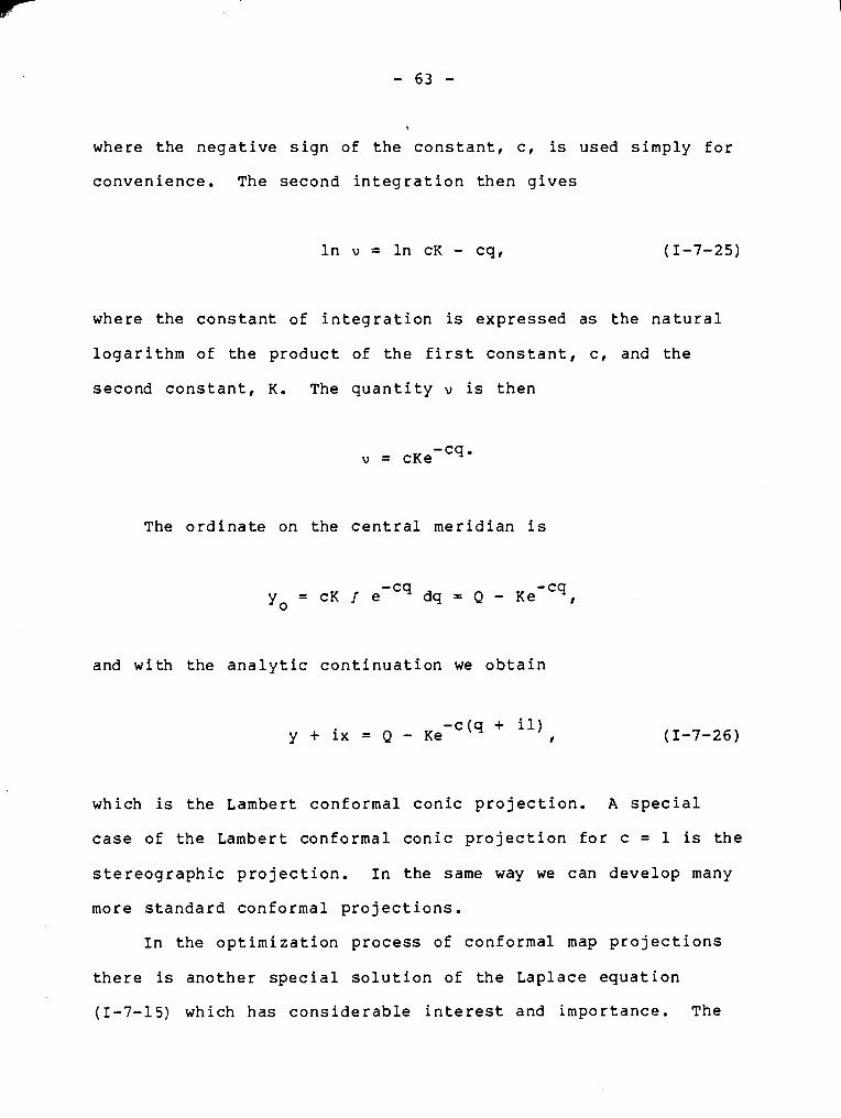
where t h e n e g a t i v e s i g n of t h e c o n s t a n t , c , is used s i m p l y f o r
c o n v e n i e n c e . The s e c o n d i n t e g r a t i o n t h e n g i v e s
I n v = I n c K - c q , (1-7-25)
where t h e c o n s t a n t of i n t e g r a t i o n is e x p r e s s e d a s t h e n a t u r a l
l o g a r i t h m of t h e p r o d u c t of t h e f i r s t c o n s t a n t , c , and t h e
s e c o n d c o n s t a n t , K. The q u a n t i t y v is t h e n
The o r d i n a t e on t h e c e n t r a l m e r i d i a n is
and w i t h t h e a n a l y t i c c o n t i n u a t i o n w e o b t a i n
- c ( q + i l ) y + i x = Q - K e I
which is t h e Lamber t c o n f o r m a l c o n i c p r o j e c t i o n . A s p e c i a l
c a s e of t h e Lambert c o n f o r m a l c o n i c p r o j e c t i o n f o r c = 1 is t h e
s t e r e o g r a p h i c p r o j e c t i o n . I n t h e same way w e can d e v e l o p many
more s t a n d a r d c o n f o r m a l p r o j e c t i o n s .
I n t h e o p t i m i z a t i o n p r o c e s s of c o n f o r m a l map p r o j e c t i o n s
t h e r e is a n o t h e r s p e c i a l s o l u t i o n of t h e L a p l a c e e q u a t i o n
(1-7-15) which h a s c o n s i d e r a b l e i n t e r e s t and i m p o r t a n c e . The

solution is given by the equation
which is a harmonic polynomial whose first five values are:
n = l q + il,
n = 2 q2 + i2ql - 12, n = 3 q3 + i3q21 - 3q12 - il3, I (1-7-28) n = 4 q4 + i4q31 - 69212 - i4q13 + 14,
n = 5 qs + i5q41 - l0q3l2 - il0q213 + 5q14 + ils.
In each of these expressions there are two groups of
uniform polynomials with coefficients related to real and
imaginary terms. Let us denote a polynomial with real
coefficients by $n and that with imaginary coefficients by en.
Each one of the polynomials qn and e n is a special
solution of the Laplace equation, thus an arbitrary linear

combina t ion of t h e two polynom'ia ls is a l s o a s o l u t i o n , i . e .
T h i s s o l u t i o n y i e l d s an i n f i n i t e s e r i e s of conformal map
p r o j e c t i o n s whose c o e f f i c i e n t s a and b . can be de t e rmined s o j I
t h a t t h e s c a l e f a c t o r m, and t h u s t h e f u n c t i o n v is o p t i m i z e d
f o r a p a r t i c u l a r mapping domain. I t can a l s o be shown t h a t
some w e l l known p r o j e c t i o n s l i k e t h e Lambert conformal c o n i c ,
Lag range ' s p r o j e c t i o n , L i t t r o v ' s p r o j e c t i o n and t h e T r a n s v e r s e
Mercator p r o j e c t i o n can be d i r e c t l y d e r i v e d from t h e e q u a t i o n
(1-7-30). I n a d d i t i o n t o t h e s e known p r o j e c t i o n s we can
deve lop many unknown b u t u s e f u l map p r o j e c t i o n s .
8. EQUIAREAL PROJECTIONS
E q u i a r e a l , o r e q u i v a l e n t map p r o j e c t i o n s a r e t h o s e i n
which t h e s c a l e of a r e a s a t eve ry p o i n t of t h e mapping domain
has one and t h e same v a l u e . For r ea sons of s i m p l i c i t y t h e
c o n s t a n t is assumed t o be e q u a l t o u n i t y . S i n c e t h e s c a l e of
a r e a s was d e f i n e d by t h e e q u a t i o n s (1-3-11) , (1-3-12) and
(1-4-11) it is e a s y t o prove t h a t t h e ma thema t i ca l c o n d i t i o n of
e q u i a r e a l p r o j e c t i o n is

This is a nonlinear partial differential equation with two
dependent variables x,y and two independent variables 4,l.
Since we have only one equation and two unknowns, the system
(1-8-1) is undetermined and has an infinite number of solu-
tions. Particular solutions can be obtained theoretically by
the integration of the above differential equation if some
additional conditions are formulated, the conditions which
clarify the relationship between dependent variables or their
connections to the independent variables. The totality of all
these conditions is again infinite, thus leading to a totality
of equiareal projections which is very difficult to derive
directly from the initial differential equation (1-8-1) in an
organized manner. However, the integration process is theoret-
ically, as well as practically, possible. Two map projections
will be developed to prove the possibility of obtaining cartog-
raphic transformation systems directly from the fundamental
condition of equiareal mappings. One of these projections is a
new equiareal projection developed by the author and the other
is a well-known map projection, Lambert's equiareal cylindric
projection.
Let us assume that the transformation formulae x = x(+,l)
and y = y(+,l) can be expressed as products of four functions
in the following way:
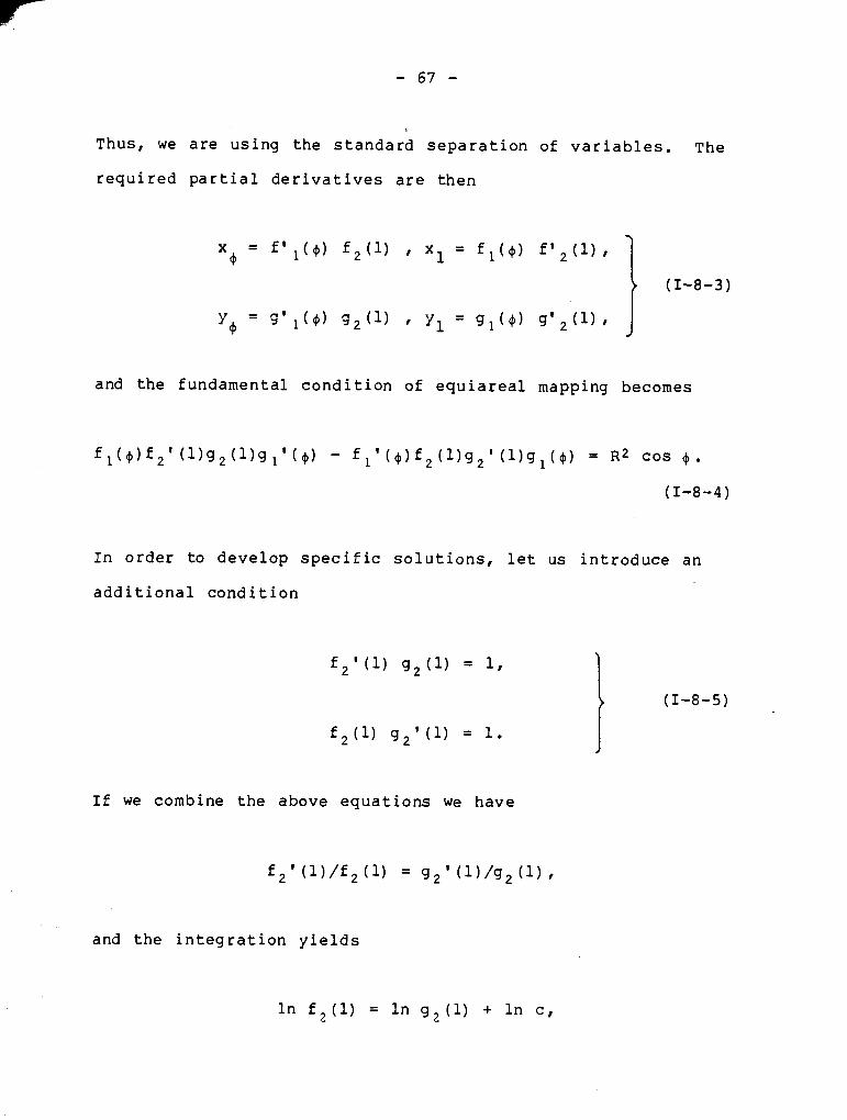
Thus, we are using the standard separation of variables. The
required partial derivatives are then
and the fundamental condition of equiareal mapping becomes
In order to develop specific solutions, let us introduce an
additional condition
f2'W g2(U = 11
f2W g2' (1) = 10
If we combine the above equations we have
•’2' (l)/f2(l) = g2' ( W g 2 (1) I
and the integration yields
In f2(1) = In g2(1) + In c,

Assuming that the constant of integration, c, is equal to unity
we finally obtain
The equality of functions f (1) and g2 (1) results in a simple
form of the first equation of (1-8-5)
f2df2 = dl,
or integrating
and finally
The fundamental equation of equiareal mappings (1-8-4) in this
particular case, with the assumptions (1-8-5) is

Let us now apply the method of undetermined coefficients. Then
the required functions f (4) and gl ( + ) have the form
f,(+) = a, cos + b, sin 4 + c,,
(1-8-9)
gl(+) = a2 cos 4 + b2 sin + + c2,
and the corresponding derivatives are
f11(4) = -a 1 sin + + bl cos +,
gll(+) = -a 2 sin + + b2 cos 4, J where a,, a2, b,, b2, cl, c2 are unknown coefficients.
Substituting the equations (1-8-9) and (1-8-10) into
(I-8-8), after some rearrangement of terms we obtain
alb2 - bla2 + cl(b2cos + - a2sin +) + c2(alsin 4 - blcos 4 )
= ~2 cos 4 .
At least one of the parameters ci must be different from
zero. The last equation will be satisfied if
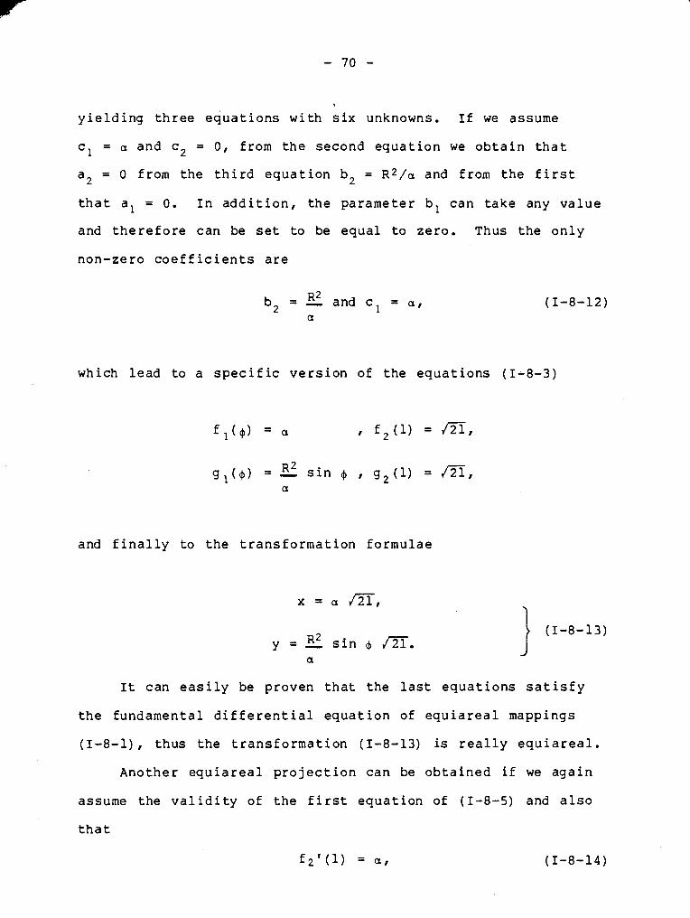
I
yielding three equations with six unknowns. If we assume
cl = a and cp = 0, from the second equation we obtain that
a2 = 0 from the third equation b2 = ~ 2 / a and from the first
that al = 0. In addition, the parameter bl can take any value
and therefore can be set to be equal to zero. Thus the only
non-zero coefficients are
- ~2 b2 - - and cl = a,
a
which lead to a specific version of the equations (1-8-3)
and finally to the transformation formulae
y = E sin ( CK. a
It can easily be proven that the last equations satisfy
the fundamental differential equation of equiareal mappings
(I-81) , thus the transformation (1-8-13) is really equiareal. Another equiareal projection can be obtained if we again
assume the validity of the first equation of (1-8-5) and also
that
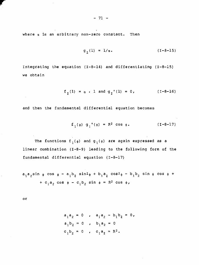
where a is an a r b i t r a r y non-zero c o n s t a n t . Then
I n t e g r a t i n g t h e e q u a t i o n (1-8-14) and d i f f e r e n t i a t i n g (1-8-15)
we o b t a i n
f , ( l ) = a . 1 and g 2 ' ( 1 ) = 0 ,
and then t h e fundamental d i f f e r e n t i a l e q u a t i o n becomes
f l ( 4 ) g l ' ( $ ) = R 2 CoS $0 (1-8-17)
The f u n c t i o n s f 1 ( + ) and g l ( 4 ) a r e a g a i n e x p r e s s e d a s a
l i n e a r combina t ion (1-8-9) l e a d i n g t o t h e fo l lowing form of t h e
fundamental d i f f e r e n t i a l e q u a t i o n (1-8-17)
a a s i n + c o s 4 - a l b 2 s i n 2 4 + b l a 2 cos24 - b l b 2 s i n 4 c o s 4 + 1 2
+ c l a 2 c o s 4 - c l b 2 s i n 4 = ~2 cos 4 ,

Thus
with the transformation formulae
~2 Y = sin 4, k
where
The equations (1-8-18) define Lambert's equiareal cylindric
projection.
The most important group of equiareal projections, from
the practical point of view, is Euler's. Euler's projections
are the equiareal mappings in which the image of the meta-
graticule constitutes an orthogonal grid. Without a loss of
generality let us take direct aspects only. Thus, in Euler's
projections the image of meridians and parallels is an orthog-
onal net of lines in the projection plane. The conditions of
Euler's projections are
p = 1 and c = O .

The orthogonality of parametric lines in the projection
indicates that the scales along meridians and parallels are the
principal scales. Thus, the conditions (1-8-20) can be written
Let us now introduce a new parameter, t, defined from the
expression (1-5-16) by
t = v2 = n2 C O S ~ + ,
which gives
ff n = - and m = 3. (1-8-23) cos + 4-F
Instead of the independent variable + we shall use another
variable, s defined as
s = sin + ( 1-8-24)
and then
ds = cos $ d$. (1-8-25)
Substituting the equations (I-8-23), (1-8-24) and (1-8-25)
into the formulae (1-5-15) we obtain
) (1-8-26) = - sin 6
Y s , y1 = 475 cos 6 4-F J

I
Conditions of differentiability xs1 = x and yS1 = yls 1s
yield
- sin - sin B E
81 - tl = fi cos B fiS + - . ts, 2 m 2ff
(1-8-27) - cos B - sin B - - -E sin B B~ + E2Ui f i 2 4 ~ 3 2 6
ts-
In order to eliminate and tS from the equation (1-8-27) 1
the first equation is multiplied by cos 8, the second by sin g
and then they are subtracted giving -- -
In the same way, one can eliminate and tl by S
multiplying the first equation of (1-8-27) by sin B, the second
by cos B and then adding them together
The differentiation of the equation (1-8-28) with respect
to 1 and of (1-8-29) with respect to s yields

The partial differential equation of the second order
(1-8-30) represents the fundamental differential equation of
Euler's projections. Superimposing some additional conditions
on the function t, we can develop, by the integration of the
fundamental equation, various types of Euler's projections.
For example, if we take a special case where t is a func-
tion of latitude only, or in our case t = t(s), then
or finally
where c and K are arbitrarily selected constants. The derived
projection is Lambert's equiareal conic projection.
If we take another special case where t is a function of
difference in longitude only, i.e.
then the equation (1-8-30) becomes
with the solution
Projections which satisfy the last equation have the
parametric grid consist of circular arcs. In a special limited
case, when the constant K is equal to zero, we obtain Lambert's
equiareal cylindric projection, the same projection that has
already been developed in (1-8-18).
Generalization of developments of equiareal projections
from the fundamental differential equation (1-8-1) requires
further systematic study of the problem. The main difficulty
is the lack of an organized series of different solutions of
the undetermined system (1-8-1). Two of many solutions using
the equations (I-8-2), derived by the author, were obtained by
a more or less trial and error approach. It requires a
mathematician with a deep insight into partial differential
equations to develop a great number of practically important
solutions.
11. OPTIMAL MAP PROJECTIONS
1. IDEAL AND BEST MAP PROJECTIONS
The problem of the determination of an optimal map
projection of the sphere, or its portion onto a plane, can be
extremely ambiguous unless the criteria for qualitative
assessments of transformation formulae are clearly and
rigorously defined. The definition of the problem is always
the most reasonable starting point for its solution. -- --
Meshcheryakov (1968) has suggested that the optimized map
projection can belong to two distinct categories. They can be
either ideal or the best transformation systems.
The concept and definition of ideal map projections was
introduced to cartography by the most important of the Russian
cartographers, V.V. Kavraiskii with the following words
(Kavraiskii, 1959):
"It is possible to find a map projection under a unique condition where, for example, the maximum deformat ion of distances for the whole mapped domain is as small as possible."
The problem of ideal map projections has not been solved. Even
its mathematical definition has not yet been clearly given.
Generally, for cartographers, the problem is too difficult

I
from the mathematical point of view, and mathematicians only
recently rediscovered mathematical cartography (Milnor, 1969).
The problem of minimization of maximal distortion, which leads
to ideal map projections, will be simply called the minimax
problem. Although the existence and uniqueness of an ideal map
projection was introduced by Kavraiskii and the existence
mathematically proven by an American mathematician, J. Milnor
( 1969), the determination of a real ideal projection for an
arbitrary domain of the sphere cannot be practically solved
unless an infinite number of conceivable transformation systems
are optimized and then compared, and this, in actuality, is an
impossible task.
Meshcheryakov (1968) recommended an alternative solution
for the problem: instead of trying to find an ideal map
projection of a certain domain, cartographers should concen-
trate on the best projections. The best projection of a given
class is the one in which deformations are at a minimum. In
other words, knowing the requirements of map users and the
shape and extent of the mapped territory, a cartographer can
predetermine the class of transformation systems and then
optimize it. The result will be the best map projection of the
particular class. By comparing several of the easily optimized
classes, or the best projections, one can make the final
decision as to which of one of the best projections will be
adopted for the mapping of the domain.

1
The criteria for the qualitative assessment of map projec-
tions, and thus the basis of the optimization process, will be
explained in the subsequent sections. For a large number of
transformation systems the optimization consists of the solu-
tion of a variational problem under the condition of extremum.
The criteria leading to such solutions are called the criteria
of the variational type (Meshcheryakov, 1 9 6 8 ) .
The optimization of conformal mappings was suggested by
various authors, but the criterion which was adopted as the
most realistic was defined by a Russian mathematician,
Chebyshev (Kavraiskii, 1 9 5 9 ) . Chebyshev stated that the best
conformal projections of a closed domain .is the one for which
the logarithm of the maximal scale is minimized. Thus, the
Chebyshev conformal projections belong to the minimax type.
The rigorous analytical determination of the Chebyshev
projection for a domain defined by an arbitrary contour line is
unknown. However, in practice, approximate solutions are
feasible and for map users they are sufficiently accurate, as
the author will show.
2. LOCAL QUALITATIVE MEASURES
Every transformation process of a closed domain of a
regular surface onto another surface whose Gaussian curvatures

differ will result in deformation of distances. By selecting
special transformation functions, areas or angles may be
preserved, but distances which are also intrinsic elements of
the original surface will always undergo a certain change.
Thus it is quite appropriate to adopt the deformation of
distances as the basic parameter for the evaluation of map
projections. Changes of angles and areas will be expressed as
functions of deformation of distances in the principal
directions.
The deformation of distances at a point, thus locally
defined, was given by the formula (1-3-2)
where k is the scale factor, a function of the position and the
direction k = ( 4 , l ,a). There are however, some additional
measures of deformations in mathematical cartography, some of
which are more and the others less important. For example, the
deformation can also be defined by the expression

1
Chebyshev, Weber and Markov (Kavraiskii, 1959) have used
the natural logarithm of the scale factor as the definition of
deformation, i.e.
The linear deformation for conical equiareal projections
is sometimes defined by the expression
v" ' s = - I (k2 - 1 ) .
2
but this definition appears to be of lesser practical
importance.
All measures of distortions of distances are functions of
the scale factor, and are thus linearly dependent, since
and thus they differ among themselves by the quantities of
second order only. In other words, for the first order term it
is irrelevant which definition of distortion is used.

I
From the author's point of view, the most natural measure
of distortion is v" = In k since its optimization in the cases
of con•’ ormal or equidistant projections automatically leads to
a minimal distortion of areas, and in the case of equidistant
and equiareal projections the optimization process guarantees
minimal deformations of angles. Analogous results are not
obtained with other definitions of linear distortion.
From the theory of distortions and the indicatrix of
Tissot we know that at every regular point of a mapping domain
the principal directions represent the directions of the
extreme scales- a and b and that every element of distortion can
be easily expressed in terms of the principal scales. For
example, the extreme angular distortion at a point in a non-
conformal projection is given by the formula
w = arc sin ((a - b)/(a + b)). 0 ,
( 11-2-61
The deformation of areas, v is defined by the equation P '

In 1861 an English astronomer, G.B. Airy, made the first
significant attempt in cartography to introduce a qualitative
measure for a combination of disortions. His measure of
quality was designed to be an equivalent to the variance in
statistics. It was defined (Airy, l86l), at first, by the
expression
a r2 = (E - 1)2 + (ab - 1)2, A
but later in the optimization process he used another version
which may be called the mean quadratic deformation of distances
where
v = a - 1 and v b = b - 1. a
Airy's two definitions of the mean quadratic deformation
(11-2-8) and (11-2-9) differ in the terms of third order only.
We can take, for example, the first definition and transform it
in the following way:

IF-
2 a - 1)2 + (ab - 1)2 = (' + va - 1) + [(I + va)(1 + vb) - 1 1 2 = (b l + v
b
The first term of the middle row in the last formula
approximates the square of the maximal angular deformation
(11-2-6) and the second term is the square of the deformation
of areas (11-2-7).
In 1897, the German cartographer A. Klingatsch generalized
the first mean quadratic deformation of Airy (11-2-8) by the
introduction of arbitrarily selected weights for the accuracy
of angles and areas. The mean quadratic deformation of
Klingatsch is then computed by the weighted mean
where p and p are positive dimensionless quantities called W P
weights. Their numerical values can be arbitrarily varied to
satisfy the specific requirements of users (Kavraiskii, 1959).
The measure of the quality of map projections by Airy
( 11-2-9) and the subsequent generalization by Klingatsch
(11-2-11) uses only the principal scales and their

, deformations. A more realistic evaluation of the deformations
of distances at a point was suggested by a German geodesist,
W. Jordan, in 1896, whose mean square deformation was defined
by the formula
I €2 = - I (k - 1)2 da, J 2r
where a is the direction angle usually reckoned from the first
principal direction (Meshcheryakov, 1969).
Kavraiskii ( 1959) recommended a small modification of the
mean square deformations of Airy and Jordan by the logarithmic
definition of linear deformation (11-2-3). Such altered mean
square deformations are called Airy-Kavraiskii and Jordan-
Kavraiskii,
and
From a theoretical point of view there is a distinct
difference between Airy's and Jordan's approaches. However,
the optimization process using either measure of quality for
mapping systems will lead to similar results whose differences
scarcely justify Jordan's much more complicated measure
(Kavraiskii, 1959).

3. QUALITATIVE MEASURES FOR DOMAINS
So far the qualitative measures of map projections have
been locally defined, since when we use one of the formulae
1 1 - 2 - (11-2-11) 1 1 - 2 - 1 2 (11-2-13) and (11-2-14) we can
compute the mean square deformation of distances at a point.
The evaluation and comparison of map projections of a closed
domain point by point in applying one of the above mentioned
expressions will generally lead to too many ambiguities with
respect to the selection of points and their distribution over
the mapped area. To alleviate these difficulties Airy (1861)
introduced the mean square error of a domain
where the integration is extended over the whole area A of the
domain.
With the logarithmic definition of distortion (11-2-3) the
criterion of Airy becomes the criterion of Airy-Kavraiskii
The optimization process leading to the minimization of
equation (11-3-2 ) will be called the optimization according to
the Airy-Kavraiskii criterion.

I
If, instead of Airy's version of the mean square
deformation, we take Jordan's formula (11-2-1 2) or the Jordan-
Kavraiskii (11-2-14) and evaluate them for the whole domain we
obtain
The optimization process, using the last formula as the
basis, is known as the optimization according to the Jordan-
Kavraiskii criterion.
In his numerical minimizations of distortions the author
will use the criterion of Airy-Kavraiskii (11-3-2).
From a theoretical point of view, the criterion of Jordan-
~avraiskii is certainly superior to the criterion of Airy-
Kavraiskii since it takes deformations in all directions around
a point and not only in the principal directions as in the
Airy-Kavraiskii formula. Practically, however, the analytical
evaluation of the integral (11-2-12) is often very difficult or
even impossible and we have to approximate it by a numerical
integration.

The i n t e g r a t i o n o f t h e mean s q u a r e d e f o r m a t i o n f o r t h e
whole a r e a i n b o t h c r i t e r i a h a s t h e same p rob lem. The boundary
c o n t o u r l i n e o f a domain is v e r y se ldom d e f i n e d by a ' n i c e '
a n a l y t i c e x p r e s s i o n . I n t h e o p t i m i z a t i o n o f mappings o f a
h e m i s p h e r e , f o r example , A i r y ( 1861 ) and Young ( 1920) had a n
a n a l y t i c a l d e f i n i t i o n o f t h e b o u n d a r y , b u t it is more u s u a l t o
d e f i n e t h e b o u n d a r y by a p o l y g o n o f d i s c r e t e p o i n t s . Even i n
t h e c a s e s o f an a n a l y t i c a l d e f i n i t i o n o f t h e boundary t h e
a n a l y t i c a l i n t e g r a t i o n may be e x t r e m e l y d i f f i c u l t or
i m p o s s i b l e . T o r e d u c e t h e p rob lem o f i n t e g r a t i o n , t h e a u t h o r
w i l l u s e t h e p r a c t i c a l p r o c e d u r e of n u m e r i c a l i n t e g r a t i o n
t h r o u g h o u t t h e r e s e a r c h .
K a v r a i s k i i ( 1 9 5 9 ) s u g g e s t e d a v e r y s i m p l e summation o f t h e
i n d i v i d u a l mean s q u a r e d e f o r m a t i o n s e v a l u a t e d a t r e g u l a r mesh
p o i n t s on t h e s p h e r e . Young ( 1 9 2 0 ) i n s i s t e d on a ' b e t t e r '
summation t a k i n g a r e g u l a r mesh on t h e p r o j e c t i o n p l a n e . F o r
r e l a t i v e l y s m a l l s i z e s o f mapping domains b o t h meshes w i l l
p r o d u c e more o r less i d e n t i c a l r e s u l t s . F o r l a r g e r domains t h e
d i f f e r e n c e s c a n be c o n s i d e r a b l e . The a u t h o r d o e s n o t see why
Young 's mesh on t h e p r o j e c t i o n p l a n e w i l l y i e l d more r e a l i s t i c
r e s u l t s , and b e c a u s e i t s f o r m a t i o n is n u m e r i c a l l y more
c o m p l i c a t e d t h e p r e f e r e n c e w i l l be g i v e n to a r e g u l a r mesh on
t h e o r i g i n a l s u r f a c e o f t h e s p h e r e .

4. OPTIMIZATION OF CONICAL PROJECTIONS
Conical map projections include those cartographic
transformations in which the metagraticule on the sphere, a
system of orthogonal coordinate lines, is projected onto a
plane in the following way. The metameridians (q = const.) are
transformed either into straight lines intersecting at a point
or parallel straight lines. Metaparallels ( 5 = const.) become
either concentric circles with the centre at the intersection
point of the projection of the metameridians, or they become
parallel straight lines orthogonal to the projection of
metameridians.
To clarify the exact meaning of the metagraticule, as
named by Wray ( l 9 7 4 ) , and its connection to the graticule, the
set of geographic coordinates (latitude @ and difference in
longitude 1 ) , let us refer to the figure 11-4-1. The metapole,
0, is usually selected to be the central point of a mapping
domain or is determined so that the central line of the mapping
territory becomes either metaparallel or the metaequator.
Great circles passing through the metapole, 0, and its
antipodal point, O', are called metameridians. The position of
a metameridian is fixed by an angle, q, called the metalongi-
tude, reckoned clockwise from the geographical central
meridian. Thus, the geographic meridian through the metapole

is the initial metameridian. Orthogonal circular curves to
metameridians are called metaparallels. They are defined by
the metalatitude, 5 , an arc length on the unit sphere between
the metaequator and the metaparallel in question.
Greenwich meridian
2
Figure 11-4-1 Graticule and metagraticule
It is clear from the figure that the metagraticule
represents a coordinate system similar to the geographic
graticule except that it is qenerally displaced on the sphere

with respect to the graticule. ~ccording to the geographic
latitude of the metapole, in conical projections we can
distinguish three different aspects:
( 1 ) 4 = " / 2 - direct aspect, 0
( 2 ) 0 < 4 < " / 2 - oblique aspect, and 0
( 3 ) 4 = 0 - transverse aspects. 0
Because the metagraticule represents an invariant frame ----
for a projection system, the first step in computation is the
transformation of the geographic coordinates into the
metacoordinates. The second step is the computation of plane
coordinates.
The metacoordinates ((,q) of a point defined by its
geographic coordinates ($,1) are obtained by the formulae of
spherical trigonometry in the spherical triangle OPA.
and
cos4 sin(X - A) tan q = 0 sin$ cos$ - sin4 c o s ~ cos(Ao-A)
0 0

I
For the t ransverse aspect ( $ o = 0 ) the l a s t formulae a re
reduced to:
s i n 6 = cos( cos(Ao-A).
sin(Ao-A) tan TI =
tan+
The f i n a l transformation i n rectangular coordinates
X = ~ ( S r n ) r Y = y ( S r ~ ) r
or i n polar coordinates
y ie lds the required cartographic project ion.
The conical pro jec t ions are subdivided in to three
subgroups of conic, azimuthal and cy l indr i c map pro jec t ions .
The general formulae of conic pro jec t ions are
x = p s i n y , y = - p c o s y ,
where

The quantity c is an arbitrary positive constant whose
numerical value is usually smaller than one. When the constant
c is exactly equal to one, we obtain azimuthal projections.
Cylindric map projections are defined by the general
expressions
where k is an arbitrary positive constant.
The principal scales coincide with the scales along the
parametric curves and for conic projections they are
For cylindric projections they become
For a reader unfamiliar with mathematical cartography the
appendix 1 contains typical grids of various conical map
projections, i .e. conic, cylindric and azimuthal mappings.
The general formulae of conic and cylindric projections,
(11-4-5) and (11-4-6) respectively, clearly indicate that there

is an infinite number of conceivable conic projections. With a
proper choice of functions p = p (6) and y = y( S ) we can derive
conformal, equiareal or equidistant or an arbitrary conical
projection. All these derivations include the determination of
two parameters. One of them is the initial constant, c or k,
and the second parameter is the constant of integration in the
solution of a particular differential equation: the equation
which specifies the character of linear distortion.
The selection of the two parameters is made in such a way
that the deformations of scale are as small as possible. In - -- -
other words, an optimization process which satisfies one of the
criteria, Airy-Kavraiskii (11-3-2) or Jordan-Kavraiskii
(11-3-4), will determine the best choice of projection
constants.
The most important conical projections are:
Lambert conformal conic projection:
where c2 is the integration constant and q is the isothermic
latitude obtained by the expression (I-7-5), which, in the case
of metalatitude becomes
q = In tan ( ~ / 4 + 5/2).
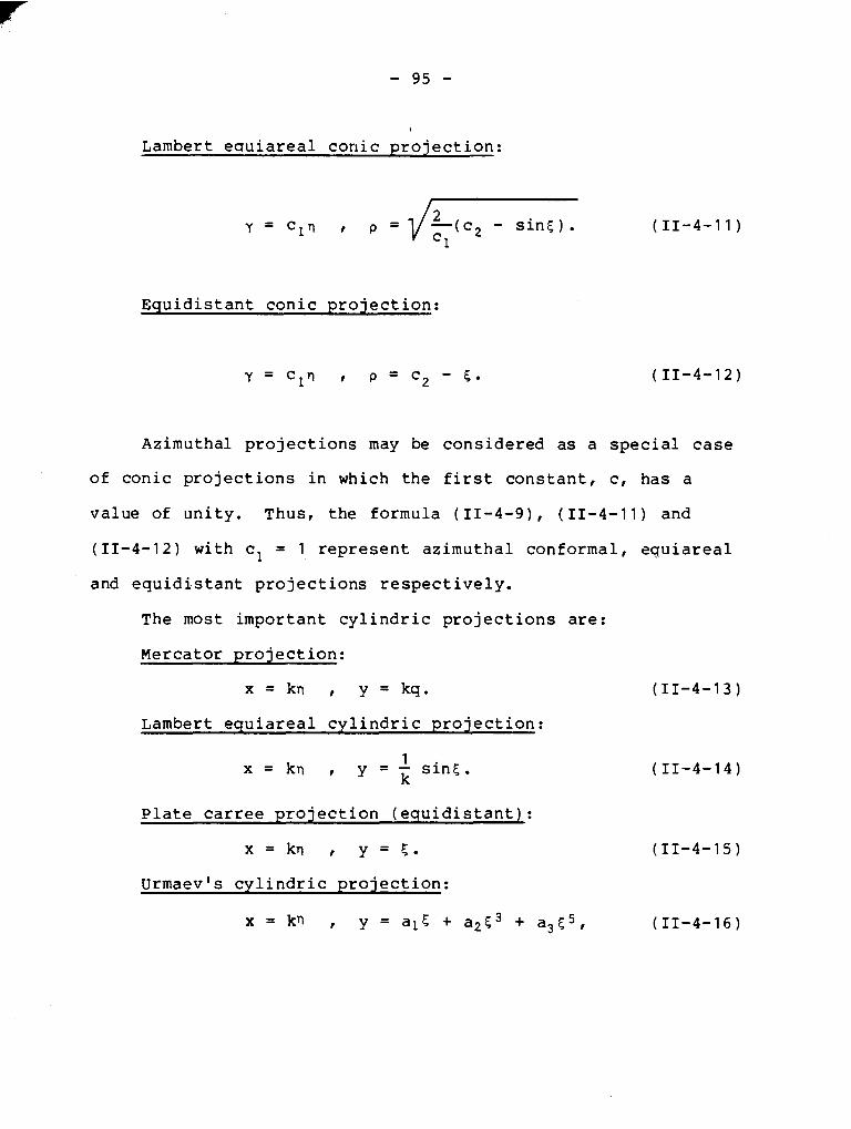
, Lambert eauiareal conic projection:
= 1/L(c2 - sing). 1
Equidistant conic projection:
Azimuthal projections may be considered as a special case
of conic projections in which the first constant, c, has a
value of unity. Thus, the formula (11-4-9), (11-4-1 1) and
(11-4-1 2) with cl = 1 represent azimuthal conformal, equiareal
and equidi.stant projections respectively.
The most important cylindric projections are:
Mercator projection:
x = k n , y = k q .
Lambert equiareal cylindric projection:
1 x = kn , y = i sing.
Plate carree projection (equidistant):
x = k n , y = C .
Urmaev's cylindric projection:
x = kn , y = a16 + a2g3 + a3{5,

I
where a!, a?, a3 are constants which can be directly computed
by defining the scale on three different metalatitudes
The constants a (i = l,2,3) can also be determined i
through optimization by applying one of the criteria of the
best projections.
Generally speaking, the optimization of conical
projections is a relatively simple problem that was solved at
the end of the nineteenth century. The detailed description of
various optimization methods can be found in (Kavraiskii,
l959), where a particular emphasis was given to the
optimization of Lambert's conformal conic projection by the
method of least squares. The optimization of one or two
constants leads to a system of one or two equations with the
same number of unknowns. The only small problem is the
mathematical definition of an optimization criterion in terms
of the required constants. The author expands the optimization
process including the simultaneous determination of the best
metagraticule for an arbitrary shaped territory and a specific

, map projection. This will enlarge the mathematical structure
by two more unknowns, the latitude and longitude of the
metapole.
Thus, in the most generalized optimization of map
projections, one of the selected optimization criteria would
have to be expressed as a function of the transformation
constants and the metagraticule. Then the numerical
approximation process will yield the best values of constants
and the best metagraticule for the particular domain and the
selected transformat ion system. - - ---
5. OPTIMIZATION OF MODIFIED PROJECTIONS
A modification of map projections is the process of
obtaining new cartographic systems from already existing map
projections. Let us assume that the rectangular coordinates
(x,y) are expressed in terms of the metagraticule ( 5 , ~ ) .
This transformation represents the initial map projection which
will be modified by the equations

where
and A and B are arbitrary constants. The functions x and y in
(11-5-2) are identical to the initial functions (11-5-1 ) except
that they are expressed in terms of new variables (u,v) ,
To simplify the modification process, the most general
modification of the metagraticule (11-5-3) will be restricted
to those modifications in which only the original metameridians
( = const.) are transformed into modified metameridians
(v = const.) and the original metaparallels (5 = const.) become
modified metaparallels (u = const.). In this case, the
transformation equations (11-5-3) are simplified to
Both of these transformations must be regular, i.e. the
Jacobian determinant of the modified transformation must be
different from zero at every point of the mapping domain,
In order to investigate the distortion parameters of the
modified map projections, we must compute the elements of the

metric tensor
The partial derivatives of the new coordinates (X ,Y) with
respect to the independent variables (5,n) can be expressed in
the following way
Then the elements of the metric tensor (11-5-6) become
with the Jacobian determinant
Taking again a unit sphere as the original surface the
distortion parameters (the scale along metameridian m, scale

along metaparallel n, parametric angle 0, and the scale of
areas p) are
p = sec u E .
- --
When the original mapping (11-5-1 ) is conformal then its
modification would preserve conformality if m = n and 0 = ~ / 2 .
From the expressions (11-5-10), (11-5-11) (11-5-12) it can
easily be seen that only an identity mapping with constants
A = B will result again in a conformal map projection. In
other words, a real modification of a transformation system
cannot retain conformality. If the original projection is
conformal its modified version can never be conformal.
When the original mapping is equiareal, its modification,
in order to be also equiareal, must satisfy the required
condition that the scale of the area is equal to unity, i.e.
du dv sec F = 1, AB(xVyu - x y ) - - u v dF dn

Since for the original equiareal mapping x y - xUyY = cos u v u
the last differential equation becomes
dv 1 cos 5 dg - = - do ABcos u d u
The resulting differential equation can be satisfied at every
point of the mapping domain only if both sides have a constant
value. Thus
At the same time the transformation of equation (11-5-14)
yields
1 cos u du = - ABC cos 5 dS ,

and its integration
1 sin u = - sin F, + K2. ABC
n
Assuming that both coordinate systems ( F , , n ) and (u,v) have the
same origin, i.e. for 5 = 0 also u = 0 and for rl = 0 also
v = 0, both integration constants K 1 and K2 become zero and the
resulting modified curvilinear coordinates become
s i n ~ , v = ~ q . sin u = - (11-5-171 ABC n
n
The first affine transformation of an equiareal conic
projection had already been suggested in 1913 by Zinger. His
modified conic equiareal projection was computed by the
formulae (Kavraiskii, 1959)
where (x,y) are the coordinates of the equiareal conic
projection and p is an arbitrary constant. A more serious
investigation of modified equiareal projections was initiated
by Siemon in 1938. However, the most thorough study of
I
modifications has been made by Wagner, (Wagner, 1941 and
Wagner, 1962). The author has adopted his theory of
modifications with the notation suggested by Franvula in his
dissertation, (Franvula, 1971).
Since constants A and B in the first equation of (11-5-17)
are arbitrarily selected values, Wagner ( 1962) recommended that
they be composed of three constants Ck, Cm, Cnin the following
way
A = ck/- I B = 1/ck= . (11-5-19)
Then the transformation formulae (11-5-2) and ( 11-5-4 )
become
and
sin u = Cmsin( , v = Cnn. ( 11-5-21 )
Thus, if the original mapping (11-5-1) is equiareal the
modification by the expressions (11-5-20) and (11-5-21 ) also
yields an equiareal transformation.

, '
The quantities Ck, Cm, Cn are positive constants whose
numerical values were subjectively selected in Wagner's work.
~rangula ( 1971 ) , however, optimized several map projections according to the criterion of Airy by varying the values of
constants. He used electronic computers and a trial-and-error
method to determine the constants in such a way that Airy's
measure of the quality EA was minimized for domains of the
whole earth and the individual hemispheres. The result of his
investigations are given in (Francula, 1971). when the
original equiareal property of the projection (11-5-1 ) is not
to be retained by the modified system, Wagner introduced a new
constant, Ca, which regulates the distortion of areas. The
transformation equations are then
For non-equiareal projections the modification of the
metagraticule can be simplified, and instead of equations
(11-5-21) we can use another set of expressions
From many equiareal projections the author has selected
the following transformations which can be modified and their
constants optimized by the criterion of Airy-Kavraiskii.

Sanson's projection:
Sanson's projection is defined as a sinusoidal equiareal
projection which satisfies three conditions: ( i) scale along
the symmetric central metameridian is constant, (ii) all other
meridians are sinusoidal curves, and (iii) the pole is
projected as a point. The original equations of the projection
are:
X = n c o s C and Y = 5 , (11-5-24 )
and the modified versions become
Y = arc sin(C sin[) . c ~ T T m n m
~ollweide' s projection:
The projection is equiareal and maps the hemisphere into a
circle of radius of 47, metameridians are symmetric ellipses
with respect to the central meridian which is a straight line.
The pole is projected as a point.
247 X = n cos YJ , Y = JZsin Y , ll
where

The modified equations of $the projection are
where
2$ + sin $ = n Cmsing . ( 11-5-28 )
Hammer's projection:
This projection was obtained by an affine transformation
of the Lambert azimuthal equiareal projection.
x = 2 6 s i n a , y = 2 s i n d c o s a , ( 11-5-29 ) 2
where
sin 5 cos a = cos cos 5 , cos a = - . (11-5-301 sin a
The modified equations become
sin d cos a , (11-5-31 ) 2
where
cos 6 = cosCnn - /1 - c2 sin25 , cos a = Cmsinc . (11-5-32) 2 m sin 6
Eckert's IV projection (elliptical):
The original equations of the projection are
where 1 Y + 2 sin Y + - sin 2 Y = (2 + R ) sin 5 2 2
The modified version of the equation is
x = C k l / z n ( 1 + cos $ ) and Y = C k m
where
sin $, (11-5-35)

6. OPTIMIZATION AND THE METHOD OF LEAST SQUARES
Let us adopt the criterion of Airy-Kavraiskii (11-3-2) as
the basis for the optimization of map projections,
' j (lnza + ln2b) dA = min. E&=xA
To simplify the writing we can introduce the abbreviations
In a = v and ln b = vb , a ( 11-6-1 )
and then the criterion becomes
dA = min
where A is the total area of the mapping domain and the
integration is extended to the whole domain. There are very
few domains in cartography which can be analytically defined,
but even for these cases it is often difficult, if not
impossible, to perform integration analytically. To alleviate
this problem the integral in the last formula will be
approximated by the finite summation

A n - - 1 z [ (va)2 $ + (vb)f] A A ~ = min , (11-6-3) E 2 ~ ~ iji i=l i 1
h
where EAK is the approximation of EAK, AA is a small but finite
portion of the domain, n is the number of area elements
covering the whole domain, and the distortion parameters
(va,vb) are numerically evaluated at the central point of each
element of the area, AA. To introduce regularity into the
computation, the mapping domain is covered by the mesh of
meridians and parallels which subdivide the domain into a large
number of spherical trapezoids. The area of such a trapezoid
limited by two parallels, and $2, and two meridians, X 1 and
X2r is obtained by the formula (Sigl, 1977)
where R is the radius of the sphere. For a small distance
between parallels we can assume that
and with the abbreviations
+ 2 - 4, = A$ and X~ - X 1 = AX ,

- 109 -
f o r a u n i t s p h e r e (R-1) f o r m u l i (11-6-4) becomes
AAi = A$ Ah COs$i ,
where ( i is t h e l a t i t u d e o f t h e c e n t r a l p o i n t o f AAi.
F u r t h e r s i m p l i f i c a t i o n is a c h i e v e d i f t h e d i f f e r e n c e s
be tween m e r i d i a n s and p a r a l l e l s a r e k e p t c o n s t a n t f o r t h e
domain. I n t h a t case
and t h e a r e a becomes
S u b s t i t u t i n g t h e l a s t e x p r e s s i o n i n t o t h e c r i t e r i o n
( 11-6-3 ) w e h a v e
n - C [ ( v a ) T + ( v b ) T ] C O S ( ~ = min , (11-6-10) E'AK - i= l 1 1

I
and since K/2A is a constant, the most suitable non-conformal
projection of a closed domain is obtained by the optimization
of the expression
n 1 [ (va) 2i + (vb); ] COS+~ = min , i=l
with the summation sign including all trapezoids which
approximate the domain. The minimization of the above
expression is nothing but a least squares problem. The unknown
parameters of a projection, metagraticule and various
constants, are to be determined in such a way that the sum of
the squares of distortions multiplied by the cosine functions
of the corresponding' latitudes is at a minimum.
The method of least squares has been known to mathematical
cartography for some time. The first suggestion that the
theory for the determination of constants in the Lambert
conformal projection be applied, was made in 1913 by Zinger
(Kavraiskii, 1959). In 1934 Kavraiskii elaborated the
evaluation of all constants of integration in the normal aspect
of conical, i.e. conic, azimuthal and cylindric projections by
the method of least squares. In 1953 Urmaev solved the problem
of a symmetric Chebyshev projection by least squares. The
result was a conformal map projection for a domain symmetric
with respect to the central meridian, the projection which did

not perfectly satisfy the boundary conditions, but where the
deviations from the boundary requirements squared and added
together gave a minimum. Finally, in 1977 Tobler suggested a
new map projection with minimized distance errors. As a result
he did not obtain a pair of analytic transformation functions
x = x(E , n ) , y = y(E ,n) but numerical values of plane
coordinates (x,y) for points whose positions on the sphere were
known. If the known points are nicely and evenly distributed
over the mapping domain it is not difficult to introduce a
numerical interpolation procedure to transform additional
points of the sphere into the plane coordinate system. The
determination of plane coordinates by the method of least
squares in Tobler ' s approach corresponds to the determination
of the most probable values of coordinates in the least squares
adjustment of geodetic control survey nets by the method of
trilateration (Mikhail, 1 9 7 6 ) .
In addition to the briefly described applications of the
method of least squares in mathematical cartography, the author
is suggesting further generalization of the optimization
process including the determination of the most suitable
metagraticule as well as other constants and parameters of
projections. The attempt will also be made to optimize
modified map projections according to the criterion of Airy-
Kavraiskii ( 11-6-1 1 ) . The method of least squares will be
applied in the following way. The distortion elements va and
Vb must be expressed as functions of unknown parameters:
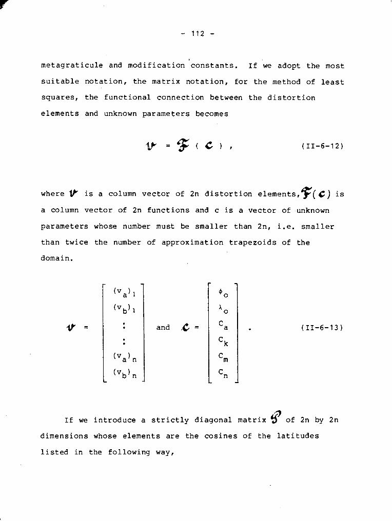
metagraticule and modification constants. If we adopt the most
suitable notation, the matrix notation, for the method of least
squares, the functional connection between the distortion
elements and unknown parameters becomes
where v is a column vector of 2n distortion elements,F(C) is
a column vector of 2n functions and c is a vector of unknown
parameters whose number must be smaller than 2n, i.e. smaller
than twice the number of approximation trapezoids of the
domain.
If we introduce a
and ,C =
strictly diagonal matrix of 2n by 2x1
dimensions whose elements are the cosines of the latitudes
listed in the following way,

the basic condition of an optimized map projection according to
the criterion of Airy-Kavraiskii (11-6-11) becomes
In this form, the equation (11-6-15) is the easily
recognizable fundamental requirement of least squares. In the
classical application of least squares for the adjustment of
physical measurements, the vector represents an array of
residual corrections of measurements and 4 is the weight matrix. In our case the weight matrix can also be modified.
If we feel that certain points of the mapping domain are more
important than others, we can assign higher weights to the more
valuable points according to some empirical rule. For example,
the density of population can serve as the weighting basis. In

, t h a t c a s e more popu la t ed a r e a s w i l l have s m a l l e r d e f o r m a t i o n s
t h a n t h e l e s s popu la t ed p o r t i o n s of t h e domain. T h e most
a p p r o p r i a t e s e l e c t i o n of w e i g h t s is a ve ry d i f f i c u l t problem
and r e q u i r e s s p e c i a l a t t e n t i o n and v e r y c a r e f u l r e s e a r c h . The
a u t h o r w i l l no t d w e l l f u r t h e r on t h e problem s i n c e it does n o t
d i r e c t l y belong t o an o b j e c t i v e o p t i m i z a t i o n p r o c e s s . I n t h i s
work t h e weight m a t r i x w i l l a lways be d e f i n e d by t h e m a t r i x
(11-6-14) , e x c e p t i n one c a s e where t h e Lambert Conformal Conic
p r o j e c t i o n is op t imized a c c o r d i n g t o t h e p o p u l a t i o n d e n s i t y a s
t h e we igh t ing bases .
I n o r d e r t o a p p l y t h e method of l e a s t s q u a r e s t h e
d i s t o r t i o n e l e m e n t s va = I n ( a ) and v b = 1 n ( b ) must be e x p r e s s e d
i n terms of t h e unknown p a r a m e t e r s , . T h i s is p robab ly t h e
main h i n d r a n c e i n t h e whole p r o c e s s . From t h e t h e o r y of
d i s t o r t i o n s i n t h e f i r s t c h a p t e r , it is known t h a t t h e semi-
a x e s of t h e i n d i c a t r i x of T i s s o t a r e computed i n t h e f o l l o w i n g
way:

The m a t h e m a t i c a l model ( 11-6-1 2 ) is g e n e r a l l y n o n l i n e a r and t o
b e used i n t h e l e a s t s q u a r e s p r o c e s s w e s h a l l l i n e a r i z e it by
t a k i n g t h e T a y l o r series
where & " is t h e v e c t o r o f a p p r o x i m a t e v a l u e s o f unknowns.
T a k i n g o n l y t h e f i r s t t w o terms i n t h i s e x p a n s i o n , t h e v e c t o r
o f c o r r e c t i o n s to t h e a p p r o x i m a t i o n s , ~ , ~ , w i l l be o b t a i n e d by
t h e method o f l e a s t s q u a r e s . The v e c t o r o f unknown p a r a m e t e r s ,
4 , is t h e n
When t h e a p p r o x i m a t e v a l u e s o f p a r a m e t e r s a r e close to t h e
s o l u t i o n , t h e c o r r e c t i o n v e c t o r is s m a l l and a l l terms o f
second o r h i g h e r o r d e r o f A & i n (11-6-17) can be n e g l e c t e d
a s b e i n g p r a c t i c a l l y i n s i g n i f i c a n t . The v e c t o r o f approxima-
t i o n s is u s u a l l y d e t e r m i n e d from p r e v i o u s e x p e r i e n c e . I t is
p a r t i c u l a r l y i m p o r t a n t to e s t a b l i s h t h e p o s i t i o n o f t h e
m e t a g r a t i c u l e r e l a t i v e l y w e l l . The b e t t e r t h e a p p r o x i m a t i o n s
t h e b e t t e r t h e end r e s u l t s w i l l be. The method o f l e a s t
s q u a r e s can a l s o be used i t e r a t i v e l y . A f t e r t h e f i r s t computa-
t i o n , t h e v e c t o r X ) c a n be r e e n t e r e d i n t o t h e c o m p u t a t i o n a s
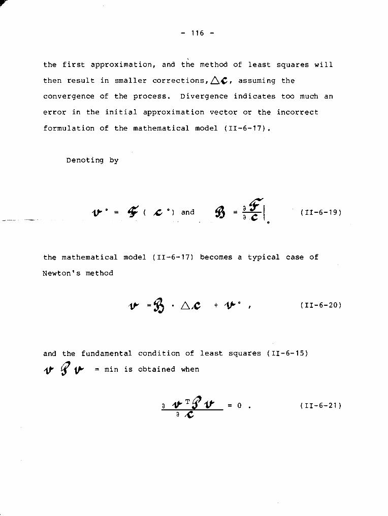
t h e f i r s t a p p r o x i m a t i o n , and t h e method o f l e a s t s q u a r e s w i l l
t h e n r e s u l t i n s m a l l e r c o r r e c t i o n s , ~ ~ , a s s u m i n g t h e
c o n v e r g e n c e o f t h e p r o c e s s . D i v e r g e n c e i n d i c a t e s t o o much a n
error i n t h e i n i t i a l a p p r o x i m a t i o n v e c t o r or t h e i n c o r r e c t
f o r m u l a t i o n of t h e m a t h e m a t i c a l model (11-6 -17) .
D e n o t i n g by
t h e m a t h e m a t i c a l model ( 11-6-17) becomes a t y p i c a l c a s e o f
N e w t o n ' s method
and t h e f u n d a m e n t a l c o n d i t i o n o f l e a s t s q u a r e s ( 11-6-1 5 )
y g v = rnin is o b t a i n e d when

Since
the partial differentiation of the above matrix equation with
respect to C yields
where
T /! x=@.& $ and a= $?9.eo . (11-6-23)

I
L i n e a r e q u a t i o n s (11-7-22) a r e c a l l e d t h e normal e q u a t i o n s
w i t h N b e i n g a n o n - s i n g u l a r s y m m e t r i c m a t r i x w i t h r e s p e c t t o
t h e p r i n c i p a l d i a g o n a l .
The s o l u t i o n o f t h e s y s t e m (11-6 -22) , f o u n d u s i n g C h o l e s k y
me thod , y i e l d s t h e v e c t o r of c o r r e c t i o n s
and t h e n , f i n a l l y , by e q u a t i o n s (11-6-18) t h e r e q u i r e d
unknowns.
A f t e r t h e d e t e r m i n a t i o n o f t h e unknowns, t h e m e a s u r e of
d i s t o r t i o n A i r y - K a v r a i s k i i is o b t a i n e d by t h e f o r m u l a
where f o r a r e g u l a r mesh t h e q u a n t i t y K is t h e p r o d u c t of t h e
d i f f e r e n c e s i n l a t i t u d e and l o n g i t u d e of t h e mesh p o i n t s , i .e.

The method of least squar;s has been by far the most
predominant approximation technique in many scientific fields.
It yields a unique solution by a very general computation
algorithm which can be applied even in the most complicated
mathematical models. If the mathematical models are linear or
linearized, the approximation algorithm consists of the
solution of linear equations whose number is equal to the
number of unknowns. If the resulting vector of corrections
& , is small, i.e. we are dealing with close
approximations, the first application of the method will give --
sufficiently good results. For larger values of /\G , the computed unknowns serve only as improved approximat ions and the
method of least squares is iteratively applied until the
difference between two successive computations of are
practically negligible.
The main difficulty in the application of least squares
for the optimization of cartographic mappings is the
linearization of the mathematical model (11-6-1 2) by the Newton
method. Analytical expressions for the deformation elements
v = In a and vb = In b in terms of the vector of unknown a
parameters are relatively complicated and their partial
differentiation with respect to the unknowns are cumbersome.
The problem can be largely simplified by the usage of one of
the available packages for a non-linear least squares fit.
Although the author has not used a single non-linear least

s q u a r e s approach it must be emphasized t h a t under c e r t a i n
c i r c u m s t a n c e s t h e y a r e t h e most e l e g a n t and e f f i c i e n t s o l u t i o n s
of t h e o p t i m i z a t i o n problem. D i f f i c u l t i e s wi th a n o n - l i n e a r
l e a s t s q u a r e s method main ly a r i s e from t h e d i f f i c u l t q u e s t i o n s
which must be d e a l t w i th i n programming of a n o n - l i n e a r
i t e r a t i v e method when t o s t o p and e i t h e r admit f a i l u r e or
d e c l a r e a c c e p t a b l e app rox ima t ion (Denn i s , 1 9 7 7 ) . I n o r d e r t o
e n s u r e convergence of i t e r a t i v e s o l u t i o n s t h e i n i t i a l app rox i -
ma t ions must be r e a s o n a b l y good. S i n c e t h e a u t h o r could n o t
f u l f i l l t h i s impor t an t i n i t i a l r equ i r emen t t o any meaningfu l
d e g r e e of accu racy t h e o p t i m i z a t i o n was performed by t h e l i n e a r
Gauss-Newton method on ly .
7. CRITERION OF CHEBYSHEV
Chebyshev fo rmula t ed i n 1856 a theorem about t h e b e s t
p r o j e c t i o n from a c l a s s of conformal p r o j e c t i o n s
(Meshcheryakov, 1969) . Conformal t r a n s f o r m a t i o n sys tems i n
which t h e changes of s c a l e m = m ( $ ,1) a r e minimized a r e c a l l e d
Chebyshev 's p r o j e c t i o n s . I n o t h e r words, t h e r a t i o of t h e
maximum and minimum s c a l e f a c t o r f o r t h e whole mapping domain
bounded by a c l o s e d con tou r l i n e w i l l be s m a l l e r t han i n any
o t h e r conformal mapping of t h e same domain. S i n c e t h e s c a l e s
i n Chebyshev 's p r o j e c t i o n s w i l l d e v i a t e a s l i t t l e a s p o s s i b l e
from u n i t y t h e l o g a r i t h m s of s c a l e s w i l l d e v i a t e a s l i t t l e a s
p o s s i b l e from ze ro .

C h e b y s h e v t s t h e o r e m ( ~ i e r n a c k i , 1965 ) s t a t e s t h a t t h e
n e c e s s a r y and s u f f i c i e n t c o n d i t i o n for a c o n f o r m a l p r o j e c t i o n
to b e l o n g t o t h e Chebyshev p r o j e c t i o n s is t h a t , a l o n g t h e
b o u n d a r y c o n t o u r of t h e domain t h e mapping s h a l l y i e l d a
c o n s t a n t scale f a c t o r .
T h u s , t h e d e t e r m i n a t i o n o f a Chebyshev p r o j e c t i o n for a
c l o s e d domain c o n s i s t s o f a s e a r c h f o r a n a n a l y t i c f u n c t i o n o f
t h e i s o t h e r m i c v a r i a b l e ( q + i l ) wh ich w i l l p r o d u c e a c o n s t a n t
scale f a c t o r a l o n g t h e b o u n d a r y o f t h e domain . ~ o i s s o n ' s
e q u a t i o n ( I - 7 - 1 8 ) , wh ich was d e v e l o p e d e a r l i e r , must h a v e a
c o n s t a n t v a l u e on t h e b o u n d a r y c o n t o u r
where f o r t h e b o u n d a r y c o n t o u r r
s e c h 2 q = c o n s t .
The g e n e r a l i t y o f t h e s o l u t i o n is n o t r e s t r i c t e d i f w e
a s sume t h e c o n s t a n t i n t h e e q u a t i o n (11-7-1) t o be z e r o . I n
t h i s c a s e , t h e d e t e r m i n a t i o n o f t h e Chebyshev p r o j e c t i o n s is
r e d u c e d to t h e s o l u t i o n o f D i r i c h l e t ' s p r o b l e m w i t h z e r o
b o u n d a r y v a l u e s (Urmaev, 1953 ) .

Chebyshev d i d n o t p r e s e n t a p r o o f o f h i s t h e o r e m . Much
l a t e r , i n 1896 , a n o t h e r R u s s i a n m a t h e m a t i c i a n and c a r t o g r a p h e r ,
D.A. G r a v e , r i g o r o u s l y p r o v e d t h e t h e o r e m . From t h a t t i m e many
a u t h o r s have c a l l e d t h e t h e o r e m t h e Chebyshev-Grave t h e o r e m o f
c o n f o r m a l mapp ings . The p r o o f f o r t h e t h e o r e m c a n be found i n
(Meshcheryakov 1 9 6 8 ) .
The d e t e r m i n a t i o n of a r e a l Chebyshev p r o j e c t i o n of a
c l o s e d domain on t h e s p h e r e c a n be s u b d i v i d e d i n t o t h r e e p a r t s .
F i r s t t h e e a r t h ' s s u r f a c e is c o n f o r m a l l y mapped o n t o a p l a n e by
t h e i s o t h e r m i c c o o r d i n a t e s - . -
where
T h i s is a c t u a l l y t h e M e r c a t o r p r o j e c t i o n o f a u n i t s p h e r e o n t o
a p l a n e w i t h t h e s c a l e f a c t o r ml = s e c 4 .
The s e c o n d s tep is t h e d e f i n i t i o n of a h a r m o n i c f u n c t i o n
which maps t h e domain i n t o a u n i t c i rc le . The t r a n s f o r m a t i o n
must be n o r m a l i z e d , so t h a t a c e r t a i n p o i n t ( q o , l o ) of t h e
domain becomes t h e c e n t r e o f t h e u n i t c i rc le . The d e f i n i t i o n

of an a n a l y t i c f u n c t i o n which d o n f o r m a l l y maps t h e domain i n t o
t h e c i r c l e is p e r f o r m e d by e i t h e r o f t w o g r o u p s o f me thods . I n
t h e f i r s t g r o u p t h e r e s u l t is an a p p r o x i m a t e a n a l y t i c f u n c t i o n ,
i .e . an a p p r o x i m a t i o n o f t h e h a r m o n i c t r a n s f o r m a t i o n f u n c t i o n
which r i g o r o u s l y s a t i s f i e s t h e boundary c o n d i t i o n . The b e s t
e x a m p l e o f t h i s k i n d o f method is t h e a p p r o x i m a t i o n method
d e v e l o p e d i n 1908 by a German e n g i n e e r , W. R i t z ( C o u r a n t and
H i l b e r t , 1 9 3 7 ) . The s e c o n d g r o u p o f me thods c o n s i s t s o f
f i n d i n g a r i g o r o u s a n a l y t i c f u n c t i o n which d o e s n o t p e r f e c t l y
s a t i s f y t h e boundary c o n d i t i o n . Thus , t h e found mapping w i l l
be f u l l y c o n f o r m a l b u t t h e P o i s s o n e q u a t i o n w i l l n o t be
c o m p l e t e l y f u l f i l l e d a l o n g t h e boundary c o n t o u r . Bo th g r o u p s
of me thods w i l l y i e l d a f u n c t i o n u=u(w) w i t h t h e s c a l e f a c t o r
The t h i r d and f i n a l s tep is t h e e s t a b l i s h m e n t o f a
t r a n s f o r m a t i o n z = z ( u ) o f t h e u n i t c i r c l e i n t o t h e c l o s e d domain
o f t h e z - p l a n e s a t i s f y i n g t h e f u n d a m e n t a l c o n d i t i o n o f
Chebyshev ' s map p r o j e c t i o n s o f t h e c o n s t a n t s c a l e f a c t o r a l o n g
t h e boundary c o n t o u r . The s c a l e f a c t o r combin ing a l l t h r e e

transformation steps is
where c is a constant.
The derivative dz/du is defined on the unit circle. At the
same time we know that
dz dz In 1-1 = v and arg - - du du - 6
Both functions, v and 6, are harmonic functions and they appear
to be conjugated. Therefore Cauchy-Riemann equations (1-7-8 )
will yield the function 6 and after that, on the unit circle,
they will also yield dz/du. By integrating the function dz/du
along the unit circle we finally obtain z=z(u) on the contour
line r , and its transformation, for example by the method of
Kantorovich (Kantorovich, Krylov, l958), yields a conformal
projection of the unit circle onto the initial domain bounded
by the contour r .
A more detailed description of the development of
Chebyshev's projections will be given in the third chapter.
An additional remark concerning the quality of Chebyshev' s
projections must be made. The scale of areas in conformal

- 125 -
, projections is obtained by the formula
p = m 2 .
Because the Chebyshev projections optimize the distortion,
defined as the natural logarithm of the scale factor, In m,
they automatically optimize the logarithm of the scale of
areas
l n p = 2 l n m .
Thus, Chebyshev's projections, of all conformal projections,
are closest to equiareal projections. Among other conformal
projections they occupy a position similar to Euler's
projections among equiareal transformations. Euler's
projections, as is well known, satisfy one of the conditions of
conformality, & = O r and are therefore closest to conformal
mappings. There is also, however, the second condition of
conformality, m=n, and if we define a class of equiareal
mappings which satisfy the second condition of conformality as
the group of equiareal projections closest to conformal, then
we have an ambiguity which does not exist with Chebyshev's
projections. Thus the uniqueness of Chebyshev's projections
among conformal projections not only does not correspond to the
position of Euler's projections among equiareal mappings, but
is in fact far greater.
111. .THE CHEBYSHEV MAP P R O J E C T I O N S
1. INTRODUCTION
The best conformal map pro jec t ions , or Chebyshev's projec-
t ions , of a closed domain by the contour l i n e I' i s the projec-
t ion i n which the r a t i o of the maximal sca le fac tor and the
minimal scale fac tor has the smallest possible value. I n order
to belong to the c l a s s of Chebyshev project ions, a conformal
mapping m u s t produce a constant scale fac tor along the boundary
contour l ine . Thus, the determination of the best conformal
transformation of a closed domain cons is t s of solving the
Laplace equation (1-7-15)
where v = m .cos 5 , for an analy t ic function of the isothermic
complex variable ( q + i l ) which w i l l y ie ld a constant scale
fac tor along the boundary, i . e .
m = const. r

I
The criterion of Chebyshev can also be defined mathemati-
cally by the Poisson equation (1-7-18)
with
The integration of the Poisson equation (111-1-2) with
boundary conditions (11-1-3 ) yields the best conformal projec-
tion.
It must be emphasized at the beginning of this chapter
that very few mapping domains in cartography have a regular and
mathematically defined contour line. The majority of mapping
areas have irregular boundaries and the rigorous determination
of Chebyshev's projections for such irregular contours is
theoretically impossible. The boundary is usually approximated
by a series of discrete points at which the boundary condition
( 111-1-3) can be rigorously satisfied.
Instead of the isothermic latitude, q, we shall introduce
a new variable, the difference of latitude, q, and the latitude
of the central point, q0
i.e.

In this way the isothermic coordinates (q,l) are normalized and
the Poisson equation (111-1-2 ) becomes
If we introduce abbreviations
the Poisson equation is transformed into
The boundary condition (111-1-3) can easily be replaced by
the zero boundary condition, i.e.

, T h i s s i m p l i f i c a t i o n of t h e boundary c o n d i t i o n is g e n e r a l l y
a c h i e v e d by t h e c o n s t r u c t i o n of a f u n c t i o n h ( q , l ) t h a t a g r e e s
w i t h t h e v a l u e s o f f u n c t i o n u on t h e boundary . Then
where z is an unknown f u n c t i o n which a l s o s a t i s f i e s t h e P o i s s o n
e q u a t i o n , however, w i t h a n o t h e r f r e e term. Thus i n a l l f u r t h e r
d i s c u s s i o n s and d e v e l o p m e n t s w e s h a l l t a k e t h e P o i s s o n e q u a t i o n
(111-1-7 w i t h t h e z e r o boundary c o n d i t i o n .
The c a l c u l u s o f v a r i a t i o n shows t h a t t h e s o l u t i o n o f t h e
P o i s s o n e q u a t i o n w i t h t h e z e r o boundary c o n d i t i o n is t h e s o l u -
t i o n o f t h e D i r i c h l e t p rob lem and is e q u i v a l e n t t o t h e minimi-
z a t i o n o f t h e D i r i c h l e t i n t e g r a l
where D is t h e p l a n e r e g i o n bounded by t h e c o n t o u r I'. I n o t h e r
words , t h e s o l u t i o n w i l l p r o v i d e u s w i t h a f u n c t i o n , u ( q , l ) ,
which is c o n t i n u o u s i n t h e domain D, t o g e t h e r w i t h its p a r t i a l
d e r i v a t i v e s o f t h e f i r s t and second orders and v a n i s h e s a l o n g
t h e c o n t o u r r .

1
~ o s t s o l u t i o n methods of t h e D i r i c h l e t problem can be
subd iv ided i n t o two fundamen ta l ly d i f f e r e n t g roups (Urmaev,
1953) . The f i r s t group c o n s i s t s of s o l u t i o n s i n which t h e
harmonic f u n c t i o n , u ( q , 1) , is approximated , bu t where t h e
approximat ion p e r f e c t l y s a t i s f i e s t h e boundary c o n d i t i o n s .
Because t h e s o l u t i o n is o n l y an approximat ion of a harmonic
f u n c t i o n , t h e P o i s s o n e q u a t i o n f o r an a r b i t r a r y p o i n t of t h e
domain w i l l no t be e x a c t l y s a t i s f i e d . The b e s t known among
t h e s e methods was deve loped by W. R i t z i n 1908 and is known
today a s t h e R i t z method. The second group of methods y i e l d s a
r i g o r o u s harmonic f u n c t i o n , t h e r e f o r e t h e Po i s son e q u a t i o n is
comple t e ly s a t i s f i e d a t e v e r y pont of t h e domain; however, t h e
boundary c o n d i t i o n s a r e no t p e r f e c t l y f u l f i l l e d . S i n c e t h e
boundary i n c a r t o g r a p h y is u s u a l l y approximated by a series of
d i s c r e t e p o i n t s , t h e boundary w i l l be a c l o s e d polygon and t h e
l i n e of c o n s t a n t s c a l e de fo rma t ion w i l l be a smooth curve which
approximates t h e polygon. L i n e s of c o n s t a n t d e f o r m a t i o n s a r e
c a l l e d i s o c o l s . Thus t h e second g roup of methods y i e l d s
conformal mappings whose i s o c o l s o n l y approximate t h e r e a l
boundary. The method of l e a s t s q u a r e s is t h e most s u i t a b l e
method i f t h e r e q u i r e d harmonic f u n c t i o n is expres sed by
harmonic po lynomia ls . The method a s c e r t a i n s t h e b e s t conformal
p r o j e c t i o n wi th t h e boundary i s o c o l app rox ima te ly f o l l o w i n g t h e
r e a l boundary.
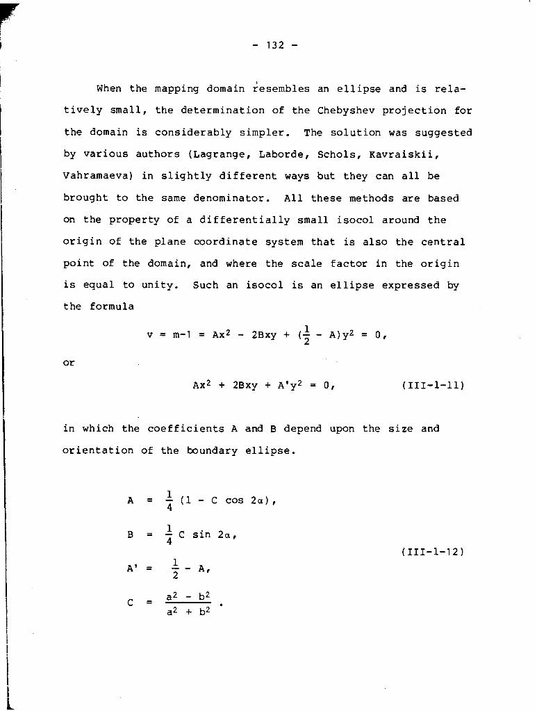
When the mapping domain iesembles an ellipse and is rela-
tively small, the determination of the Chebyshev projection for
the domain is considerably simpler. The solution was suggested
by various authors (Lagrange, Laborde, Schols, Kavraiskii,
Vahramaeva) in slightly different ways but they can all be
brought to the same denominator. All these methods are based
on the property of a differentially small isocol around the
origin of the plane coordinate system that is also the central
point of the domain, and where the scale factor in the origin
is equal to unity. Such an isocol is an ellipse expressed by
the formula
1 v = m-1 = AX^ - 2Bxy + ( - - ~ ) y ~ = 0, 2
in which the coefficients A and B depend upon the size and
orientation of the boundary ellipse.
L A = - (1 - C cos 2a), 4
1 B = - C sin 2a, 4

, The pa rame te r s a , b and a a r e t h e semi-major a x i s , t h e
semi-minor a x i s and t h e o r i e n t a t i o n a n g l e of t h e semi-major
a x i s of t h e boundary e l l i p s e , r e s p e c t i v e l y .
The r e c t a n g u l a r c o o r d i n a t e s , a c c o r d i n g t o K a v r a i s k i i ,
( 1 9 5 9 ) , a r e then ob ta ined by t h e e x p r e s s i o n s
where x, y a r e t h e Gauss ian c o o r d i n a t e s wi th r e s p e c t t o t h e
c e n t r a l p o i n t ($,, x ~ ) .
The e l l i p t i c conformal p r o j e c t i o n , i .e. , a conformal pro-
j e c t i o n wi th e l l i p t i c isocols (111-1-13) is o n l y one of s e v e r a l
examples which a r e e l a b o r a t e d i n t h e l i t e r a t u r e of ma thema t i ca l
c a r t o g r a p h y (Pav lov , 1964) . I t is g iven p u r e l y a s an i l l u s t r a -
t i o n of a s p e c i a l t ype of Chebyshev 's p r o j e c t i o n s which have
r a t h e r l i m i t e d p r a c t i c a l s i g n i f i c a n c e , a l t h o u g h t h e i r de te rmin-
a t i o n is very s imple . U n f o r t u n a t e l y , t h e boundary con tou r
l i n e s can seldom be approximated by an e l l i p s e and t h e r e f o r e
t h e merits of such a p r o j e c t i o n a r e reduced whenever t h e
boundary f l u c t u a t e s c o n s i d e r a b l y about t h e adopted e l l i p s e .

,
Various solutions of Chebyshev projections for generally
symmetric domains can be mostly found in the Russian carto-
graphic literature. For example, in 1953 N.A. Urmaev investi-
gated different ways of minimizing the Dirichlet integral by
the method of Ritz, finite difference method and the method of
least squares for conformal mapping of a symmetric spherical
trapezoid. Although a great majority of mapping domains in
geography can be seldom approximated by a symmetric spherical
trapezoid, Urmaev's work ( 1953) is an interesting contribution
to mathematical cartography. Since it is largely unknown to
North American cartographers the author decided to describe in
detail the work of Urmaev in the next three sections. The
notation is slightly modified, particularly in the method of
least squares, but the essense of Urmaev's work is preserved.
In addition to the minimization of Dirichlet's integral
for symmetric domains the author proposes the method of least
squares for a non-symmetric boundary consisting of a series of
discrete points. The development of the method is given in the
fifth section of the chapter.
It must be also mentioned that in 1973 a geodesist from
New Zealand, W. I. Reilly, developed a conformal map projection
whose isocols closely approximate the actual shape of New
Zealand. This projection to the author's knowledge is the only
real approximation of a Chebyshev projection in use at present.

l i m I ( E n ) = m n+-
A s k e t c h y d e v e l o p m e n t o f f o r m u l a e f o r t h e p r o j e c t i o n o f N e w
Z e a l a n d c a n be found i n ( R e i l l y , 1 9 7 3 ) .
2. METHOD OF RITZ
I n t h e i n t r o d u c t i o n o f t h i s c h a p t e r it was i n d i c a t e d t h a t
t h e s o l u t i o n o f t h e P o i s s o n e q u a t i o n (111-1-7) is e q u i v a l e n t to
t h e m i n i m i z a t i o n o f t h e D i r i c h l e t i n t e g r a l ( 111-1-10) ,
where D is t h e domain bounded by t h e c o n t o u r r , and t h e
r e q u i r e d f u n c t i o n u ( A q , l ) v a n i s h e s on t h e b o u n d a r y c o n t o u r .
L e t u s d e n o t e by u * ( ~ q , l ) t h e e x a c t s o l u t i o n o f t h e P o i s s o n
e q u a t i o n w i t h z e r o b o u n d a r y c o n d i t i o n s and by I ( u*) =m t h e e x a c t
v a l u e o f t h e D i r i c h l e t i n t e g r a l . I t is l o g i c a l to e x p e c t t h a t
a c o n s t r u c t e d a p p r o x i m a t i o n E ( ~ q , l ) o f t h e r e q u i r e d f u n c t i o n u*
which s a t i s f i e s t h e b o u n d a r y c o n d i t i o n s and f o r wh ich t h e v a l u e
of t h e ~ o i s s o n i n t e g r a l is close to m would be a r e l a t i v e l y
close a p p r o x i m a t i o n o f t h e unknown s o l u t i o n . I f , m o r e o v e r , o n e
can c o n s t r u c t a s e q u e n c e o f a p p r o x i m a t e s o l u t i o n s ii ( A q , l ) so n
t h a t
t h e n w e know t h a t
l i m E = u*, n n+

or t h e c o n s t r u c t e d s e q u e n c e c o n v e r g e s to t h e r e a l s o l u t i o n o f
t h e p r o b l e m , ( R e c t o r y s , 1 9 7 7 ) .
F o r t h e m i n i m i z a t i o n o f t h e D i r i c h l e t i n t e g r a l , R i t z
s u g g e s t e d a s e q u e n c e o f f u n c t i o n s d e p e n d i n g on s e v e r a l
p a r a m e t e r s
so t h a t for a l l t h e v a l u e s o f t h e p a r a m e t e r s t h e b o u n d a r y
c o n d i t i o n s a r e f u l f i l l e d . The v a l u e o f t h e D i r i c h l e t i n t e g r a l
is t h e n a f u n c t i o n of t h e unknown p a r a m e t e r s , c i , i .e .
and t h e minimum of t h e i n t e g r a l is a c h i e v e d when
a w n ) = 0 f o r i = 1 , 2 ,..., n. (111-2-5) a ci
S o l v i n g t h e s y s t e m of n e q u a t i o n s (111-2-5) w i t h n
unknowns, we o b t a i n p a r t i c u l a r v a l u e s o f p a r a m e t e r s Fi.
s u b s t i t u t i n g i n t o t h e D i r i c h l e t i n t e g r a l t h e f u n c t i o n I (F1,F2,
..., Fn) g i v e s t h e a b s o l u t e minimum. F i n a l l y , s e l e c t i n g t h e
f u n c t i o n i n t h e f a m i l y (111-2-3) c o r r e s p o n d i n g to t h e computed
v a l u e s of t h e p a r a m e t e r s , T i , w e c o n s t r u c t t h e r e q u i r e d
a p p r o x i m a t e s o l u t i o n

In 1953 the Russian geodesist N.A. Urmaev was the first
to recommend the application of the Ritz method for conformal
projections of symmetric domains with respect to the y-axis of
the plane coordinate system. He suggested that the sequence
(111-2-3) be defined as a linear combination of independent
functions q ( = 0 , 2 , n ) , i.e.
Functions qi must be continuous inside the domain and they
must vanish along the contour line. When the linear combina-
tion (111-2-7) is substituted into the Dirichlet integral (III-
2-4) it yields a quadratic function of coefficients ai whose
partial differentiation (111-2-5) results in a set of n linear
equations with n unknowns which can easily be solved. The
simplicity of the solution of the system (111-2-5) appears to
be the main reason for the suggested formulation of the
function un.
The domain of Urmaev's investigations was a spherical
trapezoid bounded by the isothermic latitudes ql and q2? and
the difference in longitude 1. If we define the auxiliary
quantities

then the function, u, must vanish for values of <=&a and l=+b.
Among many, the following family of functions will satisfy the
boundary conditions for any values of parameters c,
The above series assumes symmetry with respect to the 1-
axis of the curvilinear coordinate system and thus all odd-
power terms of 1 disappear.
Let us take the second of these expressions as our
approximation,
u = (a2-~q2)(b2-12)(cl+c2~q) (111-2-10)
The partial derivatives of the selected function with
respect to the independent variables (q,l) are
and the corresponding squares
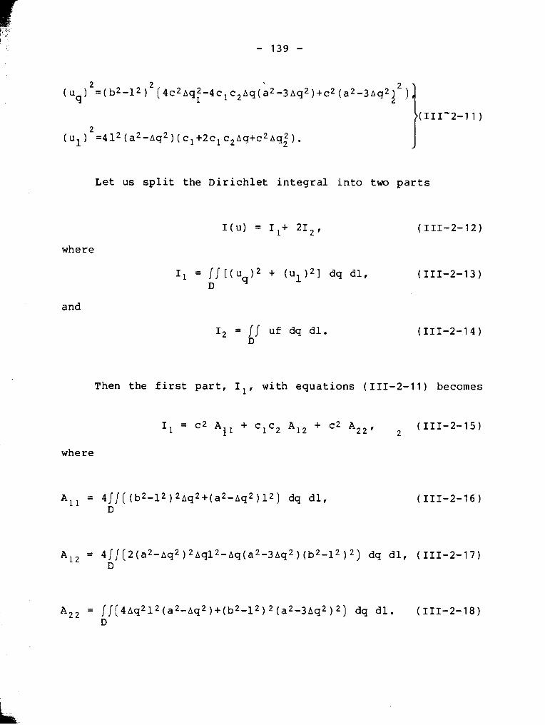
Let us split the Dirichlet integral into two parts
where
and
= / / uf dq dl. D
Then the first part, I with equations ( 111-2-1 1 ) becomes
I1 = c2 A + clc2 A12 + c2 A22, i 1 (111-2-15) 2
where
A1 1 = 4//((b2-12)2~q2+(a2-~q2)12) dq dl, D
A,, = 4//(2(a2-hq2) 2~q12-~q(a 2-3~q2)(b2-12)2) dq dl, (111-2-17) D
A,, = //(4hq212 (a2-hq2)+(b2-12) (a2-3hq2) 2, dq dl. (111-2-18) D

The second part of the Dirichlet integral, 12, can also be
expressed as the sum of two integrals M1 and M2.
where
M1 = II((a2-Aq2)(b2-12) f dq dl, (111-2-20) D
and
M2 = //((a2-Aq2)(b2-12)Aq f dq dl. (111-2-21) D
The evaluations of integrals Aij i f = 1 2 ) in limits from
-a to +a and from -b to +b can easily be performed. See, for
example (Kantovovich-Krylov, 1958). Their values are
In both integrals, MI and M2, we have the evaluation of
therefore M1 and M2 , taking into account ( 111-2-23), are
transformed into

and
Let us now introduce new symbols
+a 1 +a 1 +a K = I f dq, K1 = - J f Aq dq, K2 = - 0 -a a -a a2-a I f m2 dq, 1
With these abbreviations the integrals, M1 and M2, become
4 Ml = - a2b3 (K - K2), 0
( 111-2-27) 3
and
The only remaining problem is the computation of integrals
Ki (i=0,1,2,3). Their determination is done in the following
way

or, knowing the relationship between the metalatitude and the
corresponding isothermic latitude we have
Other values of Ki (i=1,2,3) are derived from the
integration by parts
1 K1 = tanhq2 + tanhql + - In cosh qL
a cosh q2
or in terms of the metalatitude

1 + a K 2 = - ( a 2 ( t a n h q 2 - t a n h q l ) - 2[Aq l n c o s h ( q o + a q ) ] +
a2 -a
2 c o s h q, K 2 = t a n h q 2 - t a n h ql - - I n
2 + - No,
a c o s h q l a2
where
N = J I n cosh (qo+Aq) dq. 0 -a
The f i n a l i n t e g r a l K3 is s o l v e d by a s i m i l a r way, and
+a -3 1 t a n h ( q o + b q ) b q 2 d q ,
- a

K3 = t a n h q2 + t a n h q 1 + - 3 i n Gosh q 1 + 2 N~ , a c o s h q2 a3
where
With t h e m e t a l a t i t u d e t h e i n t e g r a l K 3 becomes
-- --.-- -
The v a l u e s o f i n t e g r a l s N 1 and N2 c a n be d e t e r m i n e d by o n e
o f t h e n u m e r i c a l p r o c e d u r e s . It is s u f f i c i e n t to e v a l u a t e t h e
f u n c t i o n s nq, l n ( c o s h q ) , where ~ q = q - q o , i n l i m i t s be tween q l
and q2 and t h e n a p p l y an i n t e g r a t i o n f o r m u l a .
The ~ i r i c h l e t i n t e g r a l ( 111-2-12) w i t h e x p r e s s i o n s ( I I I - 2 -
1 5 ) and ( 1 1 1 - 2 - 1 9 ) , knowing t h a t A 1 2 = 0 , becomes
and i ts minimum o c c u r s when
and

C1 = -Ml/Al and c2 = -M2 /Az2 . (111-2-40)
Formula (111-2-10) w i l l p r o v i d e u s w i t h v a l u e s o f t h e
r e q u i r e d f u n c t i o n , u = l n ( m ) , f o r v a r i o u s p o i n t s o f t h e mapping
domain.
The whole d e s c r i b e d a p p r o a c h , s u g g e s t e d and d e v e l o p e d by
urmaev, is a p p l i c a b l e when t h e mapping domain is a s p h e r i c a l
t r a p e z o i d . The most g e n e r a l d e f i n i t i o n o f t h e f a m i l y o f func-
t i o n s e q u i v a l e n t t o (111-2-9) c a n n o t be f o r m u l a t e d f o r a n
a r b i t r a r y boundary c o n s i s t i n g o f a series o f d i s c r e t e p o i n t s .
F o r a c i r c u l a r domain w i t h t h e c e n t r e a t t h e o r i g i n o f t h e
i s o t h e r m i c c o o r d i n a t e s y s t e m , ( A q , l ) , t h e a u t h o r s u g g e s t s
a n o t h e r f a m i l y o f f u n c t i o n s
( r 2 - ~ q 2 - 1 2 ) ( c 1 + c 2 d q + c 3 ~ q 2 ) , ... etc . ,
where r is t h e r a d i u s o f t h e c i r c u l a r s p e r i c a l domain e x p r e s s e d
i n r a d i a n measure .
When t h e boundary c o n s i s t s o f a convex , non-symmetr ic
po lygon o f m d i s c r e t e p o i n t s , t h e f a m i l y o f f u n c t i o n s is

Thus it is obvious that, for a circular cap, (111-2-41 )
has a similar symmetric form as the system (111-2-9) and deri-
vations with evaluations of required integrals can be performed
in a similar manner. However, the system (111-2-42) with a
slightly larger number of points is very difficult to solve.
In addition to the computational disadvantage, the polygon must
be strictly convex, i.e., every straight line which defines a
section of the boundary between any two successive points of
the boundary must be completely outside the mapping domain.
Because of all these complications cartographers have never
applied the ~ i t z method, at least to the author's knowledge,
for a non-symmetric arbitrary boundary. The complexity of
integration discourages even the most enthusiastic carto-
grapher. The integration of M1 and M2 could be performed
numerically rather than analytically which would introduce a

I
c e r t a i n r e d u c t i o n of problems. I t is a l s o impor t an t t o empha-
s i z e t h a t b e t t e r app rox ima t ions t o t h e t r u e c o n f o r m a l i t y a r e
ach ieved when more te rms i n (111-2-9) a r e used, which a g a i n
i n c r e a s e s t h e compu ta t iona l d i f f i c u l t i e s .
3. THE METHOD OF FINITE DIFFERENCES
The R i t z method is no t t h e on ly method of f i n d i n g a
f u n c t i o n , u ( q , l ) , a s an approximate s o l u t i o n of t h e Po i s son - - -
e q u a t i o n wi th z e r o boundary c o n d i t i o n s . Urmaev ( 1953) a l s o
s u g g e s t e d t h e a p p l i c a t i o n of t h e f i n i t e d i f f e r e n c e method. The
method is b a s i c a l l y v e r y s imp le b u t it a l s o assumes symmetry
abou t t h e q-ax is , which c e r t a i n l y d e c r e a s e s i ts range of
a p p l i c a t i o n .
L e t us assume t h a t t h e domain is subd iv ided i n t h e d i r e c -
t i o n of isometric l a t i t u d e i n t o ( q 2 - q l ) / h rows, where h is
t h e width of a row, and i n t h e d i r e c t i o n of l o n g i t u d e i n t o
( 1 2 - l l ) / k columns, where k is t h e wid th of a column.
The f u n c t i o n u depends upon two v a r i a b l e s , q and 1. A t
an a r b i t r a r y p o i n t of t h e domain t h e T a y l o r expans ion y i e l d s

L e t us t a k e f i v e n e i g h b o u r i n g p o i n t s , a s shown i n f i g u r e
111-3-1, and e x p r e s s t h e v a l u e s o f t h e f u n c t i o n u a t f o u r
p o i n t s i n terms of t h e c e n t r a l p o i n t .
F i g u r e 111-3-1 A s e c t i o n of t h e g r i d

When t h e above e q u a t i o n s a r e added i n p a i r s , i .e . , t h e
f i r s t t o t h e t h i r d and t h e second t o t h e f o u r t h w e o b t a i n
The f i r s t e q u a t i o n of (111-3-3) is d i v i d e d now by h e , t h e
second by k2 and t h e r e s u l t s a r e added

where R is t h e r e m a i n d e r which ' c o n t a i n s t h e terms o f t h e f o u r t h
and h i g h e r o r d e r s of h and k.
From t h e P o i s s o n e q u a t i o n ( 111-1-2) we h a v e
and t h e r e f o r e e q u a t i o n (111-3-4) becomes
where
p = - k 2 and f ' = k 2 s e c h 2 q . (111-3-6) h2
I n t h i s manner t h e r i g o r o u s s o l u t i o n o f t h e P o i s s o n
e q u a t i o n is s u b s t i t u t e d by an a p p r o x i m a t e n u m e r i c a l s o l u t i o n .
A t e v e r y p o i n t o f t h e s y m m e t r i c mapping domain , s t a r t i n g f rom
t h e b o u n d a r y where t h e v a l u e s of f u n c t i o n u ( q , l ) a r e known, we
c a n write a compute r program w i t h e a s e , b u t f o r a s y m m e t r i c
b o u n d a r y w i t h r e s p e c t to one c o o r d i n a t e a x i s o n l y , t h e p rogram
can be v e r y complex .

, 4. SYMMETRIC CHEBYSHEV PROJECTIONS BY LEAST SQUARES
The R i t z and f i n i t e d i f f e r e n c e methods s o l v e t h e P o i s s o n
e q u a t i o n (1-7-18) w i t h z e r o boundary c o n d i t i o n s by a p p r o x i -
m a t i n g a t r u e ha rmonic f u n c t i o n . Thus , s t r i c t l y s p e a k i n g , t h e
r e s u l t s o f t h e t w o methods a r e n o t e x a c t c o n f o r m a l mapp ings b u t
a p p r o x i m a t i o n s o n l y . Us ing t h e r e s u l t s i n t h e P o i s s o n e q u a t i o n
w e w i l l o b t a i n some d i s c r e p a n c i e s , i.e., t h e P o i s s o n e q u a t i o n
w i l l n o t be e x a c t l y s a t i s f i e d e x c e p t a l o n g t h e boundary c o n t o u r
o f t h e domain. L e t us now t a k e t h e o p p o s i t e a p p r o a c h and
d e v e l o p e x a c t h a r m o n i c f u n c t i o n s which y i e l d t r u e c o n f o r m a l
mapp ings b u t o n l y a p p r o x i m a t e l y s a t i s f y t h e boundary c o n d i -
t i o n s . I n o r d e r t o e l i m i n a t e l a r g e d i s c r e p a n c i e s i n t h e z e r o
b o u n d a r y c o n d i t i o n s , t h e method o f l e a s t s q u a r e s w i l l be
a p p l i e d . Once t h e e x a c t ha rmonic f u n c t i o n is s e l e c t e d , t h e
method of l e a s t s q u a r e s w i l l y i e l d c o e f f i c i e n t s r e l a t e d to t h e
selected harmonic f u n c t i o n d e t e r m i n e d i n s u c h a way t h a t t h e
d i s c r e p a n c i e s of t h e z e r o boundary c o n d i t i o n s s q u a r e d and added
t o g e t h e r w i l l g i v e u s a minimum. The e a s i e s t h a r m o n i c f u n c t i o n
for t h e s e p u r p o s e s is a ha rmonic p o l y n o m i a l (1-7-27 ) . W e
s h a l l assume symmetry o f t h e boundary c o n t o u r i n t h e f i r s t c a s e
and non-symmetr ic c a s e s w i l l be d e a l t w i t h i n t h e s u b s e q u e n t
s e c t i o n .
The q u a n t i t y v a s d e f i n e d by t h e e q u a t i o n (1-7-13) is a
complex f u n c t i o n , t h u s t h e n a t u r a l l o g a r i t h m can be e x p r e s s e d
by ha rmonic p o l y n o m i a l (1-7-29)

I n m = a + a l q l + a 2 q 2 + ... + akqk + I n c o s h q. (111-4 -1 ) 0
The c o e f f i c i e n t s a i , f o r i = O , l , . . . . . . , k , are d e t e r m i n e d by
t h e method o f l e a s t s q u a r e s f rom t h e f u n d a m e n t a l c o n d i t i o n o f
l eas t s q u a r e s n
( I n m i ) 2 = min , i=l
where n is t h e number of d iscre te p o i n t s wh ich a p p r o x i m a t e t h e
b o u n d a r y c o n t o u r . The number o f f i x e d b o u n d a r y p o i n t s m u s t be
l a r g e r t h a n t h e number o f unknown c o e f f i c i e n t s , i . e . ,
L e t u s a g a i n u s e m a t r i x n o t a t i o n , t h e most s u i t a b l e t y p e
o f n o t a t i o n f o r t h e method o f l e a s t s q u a r e s , i n wh ich t h e
f u n d a m e n t a l e q u a t i o n o f t h e m a t h e m a t i c a l model ( 111-4-1 )
o b t a i n s t h e fo rm
w h e r e
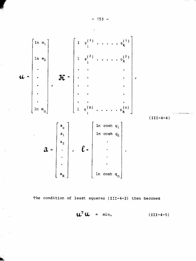
The c o n d i t i o n o f l e a s t squares (111-4-2) then becomes
uTu = min, (111-4-5)

which t a k e s p l a c e when t h e f i r s t d e r i v a t i v e of U ~ C T S ( w i t h
r e s p e c t t o t h e v e c t o r o f t h e unknowns, a , is e q u a l t o z e r o ,
i .e . ,
T a k i n g t h e m a t h e m a t i c a l model (111-4-3) we can wr i t e
and t h e d e r i v a t i v e of t h e above e x p r e s s i o n is
or f i n a l l y ,
where
Y P T -4 3c = JL and b = J; b (111-4-9) .+p T -

The s o l u t i o n of t h e system of normal e q u a t i o n s (111-4-8)
y i e l d s t h e v e c t o r of unknowns
A s a measure of q u a l i t y of t h e l e a s t s q u a r e s f i t , w e can
u s e t h e v a r i a n c e from s t o c h a s t i c ma thema t i ca l models
The h i g h e r t h e deg ree of harmonic po lynomia ls , t h e b e t t e r
t h e f i t t h e s o l u t i o n w i l l have. I f w e keep n, t h e number of
f i x e d boundary p o i n t s , c o n s t a n t , t h e i n c r e a s e of t h e o r d e r o f
t h e po lynomia l , k, r e s u l t s i n a s m a l l e r v a l u e of t h e denomina-
t o r i n ( 1 1 1 - 4 - 1 1 ) and a l s o , n a t u r a l l y , i n a s m a l l e r v a l u e o f
uTu . Thus, t h e r e must be an o p t i m a l v a l u e of k which w i l l
y i e l d t h e s m a l l e s t v a r i a n c e . To o p t i m i z e t h e o r d e r k, t h e
a u t h o r sees no o t h e r way than a t r i a l - a n d - e r r o r approach.
S e v e r a l o r d e r s of k should be t aken and t h e s o l u t i o n s eva lu -
a t e d . When t h e d i f f e r e n c e s i n t h e s c a l e f a c t o r , m, become
p r a c t i c a l l y i n s i g n i f i c a n t u s ing k-th and ( k + l ) - s t o r d e r of t h e
harmonic po lynomia l , f u r t h e r i n c r e a s e s of t h e o r d e r a r e mean-
i n g l e s s . I f , however, t h e boundary c o n d i t i o n s a r e weighted
more, t h e s m a l l e s t v a l u e of v a r i a n c e , u 2 , w i l l i n d i c a t e t h e
b e s t o r d e r of t h e po lynomia l .

I
With known coefficients, ai, we can compute the logarithm
of the scale factor and, thus, the scale factor at every point
of the mapping domain
(ao+al$l+. ..a $ +In cosh q) m = e k k .
The rectangular coordinates (x,y) of a Chebyshev projec-
tion determined in this way for a symmetric domain are also
computed by a harmonic polynomial
where
If we separate the real and imaginary parts we obtain the
formulae k
The unknown coefficients A for i=O, 1,. . , ,k, are obtained if
from the expression (1-7-19)

The f i r s t d e r i v a t i v e o f t h e a b o v e e q u a t i o n w i t h r e s p e c t t o
t h e i s o t h e r m i c l a t i t u d e y i e l d s t h e f u n c t i o n v e t t h u s
S i n c e f u n c t i o n v c a n a lso be d e t e r m i n e d f rom (111-4-1) by 0
t h e f o r m u l a
it s u f f i c e s to d e t e r m i n e v O v a l u e s a t k d i f f e r e n t p o i n t s a l o n g
t h e c e n t r a l m e r i d i a n and s u b s t i t u t e them i n t o (111-4 -17) . The
r e s u l t is k l i n e a r e q u a t i o n s w i t h k unknowns Ai ( i = 1 , 2 , . .. , k ) .
I n t h e m a t r i x form we h a v e
w h e r e

The s o l u t i o n of t h e s y s t e m (111-4-19) y i e l d s t h e f i n a l
unknowns, Ai . The e l e m e n t s o f t h e m a t r i x X c a n be d e t e r m i n e d d i r e c t l y
from t h e e q u a t i o n s (1-7-29) which i n o u r c a s e a r e

,
In the same way we can compute (for j=lt2,. . . #k)
However, with electronic computers it is much more
suitable to use the recursion relations. With the initial
values
other elements are
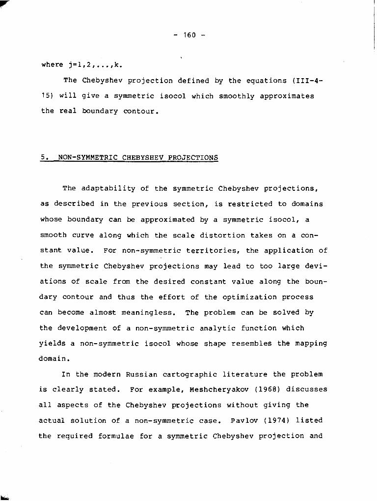
where j=1,2, ..., k. The Chebyshev projection defined by the equations (III-4-
15) will give a symmetric isocol which smoothly approximates
the real boundary contour.
5. NON-SYMMETRIC CHEBYSHEV PROJECTIONS
The adaptability of the symmetric Chebyshev projections,
as described in the previous section, is restricted to domains
whose boundary can be approximated by a symmetric isocol, a
smooth curve along which the scale distortion takes on a con-
stant value. For non-symmetric territories, the application of
the symmetric Chebyshev projections may lead to too large devi-
ations of scale from the desired constant value along the boun-
dary contour and thus the effort of the optimization process
can become almost meaningless. The problem can be solved by
the development of a non-symmetric analytic function which
yields a non-symmetric isocol whose shape resembles the mapping
domain.
In the modern Russian cartographic literature the problem
is clearly stated. For example, Meshcheryakov (1968) discusses
all aspects of the Chebyshev projections without giving the
actual solution of a non-symmetric case. Pavlov (1974) listed
the required formulae for a symmetric Chebyshev project ion and
I
mentioned non-symmetric g e n e r a l i z a t i o n s by t h e method of
Vahramaeva, w i thou t d e s c r i b i n g t h e a c t u a l p r o c e s s or g i v i n g any
mathemat ica l e x p r e s s i o n . The a u t h o r was u n s u c c e s s f u l i n
o r i g i n a l l y o b t a i n i n g any r e f e r e n c e s w i th a d e t a i l e d e x p l a n a t i o n
of t h e method used by Vahramaeva. With t h e assumpt ion t h a t
Vahramaeva a p p l i e d non-symmetric harmonic po lynomia l s (1-7-30)
t h e au tho r has deve loped a l l t h e r e q u i r e d formulae which, he
had b e l i e v e d , c o n s t i t u t e t h e method of Vahramaeva. However,
a f t e r r e a d i n g t h e f i r s t v e r s i o n of t h e t h e s i s , D r . T o b l e r s e n t
t o t h e a u t h o r t h e E n g l i s h t r a n s l a t i o n of an a r t i c l e by
Vahramaeva. The deve loped formulae by t h e a u t h o r do n o t
resemble t h e work of Vahramaeva.
L e t us t a k e t h e harmonic po lynomia l (1-7-30) and write it
i n t h e form
Using t h e d e f i n i t i o n of f u n c t i o n v i n (1-7-13) t h e l a s t
fo rmula can be t r ans fo rmed i n t o
I n m = a + a l + l + ... 0 + akqk +
+ b l o l + ... + b k o k + i n cosh q ,

where a ( 0 1 . . . k ) and b ( = 1 , 2 k) a r e unknown i i
c o e f f i c i e n t s to be d e t e r m i n e d by t h e method of l e a s t s q u a r e s
t h u s s a t i s f y i n g t h e f u n d a m e n t a l r e q u i r e m e n t ( 111-4-2)
n 1 ( I n m i ) 2 = m i n ,
i=l
where n is t h e number of d i s c r e t e p o i n t s which a p p r o x i m a t e t h e
boundary . The number n m u s t be l a r g e r t h a n t h e number o f
unknown c o e f f i e n t s , i .e.,
~ e t us a g a i n i n t r o d u c e a s imi l a r m a t r i x n o t a t i o n t o t h a t
i n t h e p r e v i o u s s e c t i o n
tT = [ I n c o s h ql l n c o s h q2 . . i n c o s h q n ]

where i ( i ) a n d o ( ~ ) , for j= l , . . . ,k and 1 , . . n a r e computed b y j j
t h e e x p r e s s i o n s (111-4-22) and (111-4-23) r e s p e c t i v e l y or by
t h e r e c u r s i o n f o r m u l a e ( 111-4-24) .
The v e c t o r o f unknowns & is t h e n
Compared to t h e d e t e r m i n a t i o n of t h e s y m m e t r i c Chebyshev
p r o j e c t i o n s , t h e d e v e l o p m e n t o f non-symmetr ic f o r m u l a e up t o
now is, more or less, i d e n t i c a l t o t h e f o r m e r e x c e p t t h a t t h e
m a t r i x 3f, a l s o i n c l u d e s t h e terms of t h e i m a g i n a r y p a r t o f t h e
ha rmonic p o l y n o m i a l and t h e v e c t o r of t h e unknown c o e f f i c i e n t s
c o n s i s t s o f p a r a m e t e r s a i and bi where i=l,. . . , k . T h e o r e t -
i c a l l y t h e o r d e r of p o l y n o m i a l s p i and O d o n o t need to be t h e j
same, b u t t h r o u g h o u t t h i s work, f o r r e a s o n s of s i m p l i c i t y , t h e
a u t h o r a s s u m e s t h a t i , j= l , . . . , k .

With known c o e f f i c i e n t s a i b i , a s c e r t a i n e d f rom t h e f
boundary c o n d i t i o n s , t h e a n a l y t i c c o n t i n u a t i o n e n a b l e s u s t o
compute t h e l o g a r i t h m o f t h e scale a n d , t h u s , t h e s c a l e i t s e l f
a t e v e r y p o i n t o f t h e mapping domain by t h e f o r m u l a ( 111-5-2) . L e t u s now e x p r e s s t h e same f o r m u l a as t h e sum o f two v e c t o r
p r o d u c t s and t h e l o g a r i t h m of t h e c o s i n e h y p e r b o l i c f u n c t i o n o f
t h e i s o t h e r m i c l a t i t u d e ,
l n m = aTQ + b T $ + a , + I n c o s h q
where
a T = [ a , a , . . . . . . . a k ] ,
I n t h e same way t h e f o r m u l a (111-5-1) becomes
and

We have already seen that the plane rectangular coordin-
ates (x,y) obtained by a conformal mapping are conjugated har-
monic functions of the isothermic coordinates which, thus,
satisfy the Cauchy-Riemann equations (1-7-8 ) . Therefore, if
the selected analytic function of conformal mapping is a har-
monic polynomial, the rectangular coordinates will be computed
by the pair of functions
where
The coefficients Ai, Bi, for 1 , . . k , are unknown and
will be obtained from the fundamental equations of map projec-
tions (1-5-15) and (1-5-19). Since we are dealing with a con-
formal mapping in which there is no distortion of the para-
metric angle, E = O , and the scale factor is constant at a point,
m=n, the equations (1-5-1 5) become

- 166 -
x = -m s i n $ , 4
X I = V COS $ ,
yb = m cos , y l = v s i n 6 ,
where
v = m cos 9 = m s e c h q. (111-5-17)
The r e l a t i o n s h i p between t h e g e o g r a p h i c and t h e i s o t h e r m i c
l a t i t u d e ( I - 7 - 1 2 ) , where dq/d$ = sec 6 = c o s h q , e n a b l e s u s t o
t r a n s f o r m t h e e x p r e s s i o n s ( 111-5-1 6 ) i n t o
x = -v s i n 8 , 9
X1 = v COS 8 ,
Yq = v cos 8 , y1 = v s i n 8 .
L e t us now d i f f e r e n t i a t e t h e r e c t a n g u l a r c o o r d i n a t e s ( x , y )
a s e x p r e s s e d by (111-5-14) w i t h respect to t h e i s o t h e r m i c l a t i -
t u d e q ,

b e a r i n g i n mind t h a t and a r e v e c t o r s of c o n j u g a t e d
harmonic po lynomia ls w h i c h must s a t i s f y t h e Cauchy-Riemann
e q u a t i o n s
L e t us deno te t h e d e r i v a t i v e s of v e c t o r s and $ w i t h
r e s p e c t t o t h e i s o t h e r m i c l a t i t u d e by v e c t o r s and Y , r e s p e c t i v e l y ,
where
Thus t h e i n d i v i d u a l e l emen t s of v e c t o r s f and a r e
o b t a i n e d by t h e formulae

= , j j l *I'= { v j = j o j - , ] for j = l , ..., k
w h e r e
The c o n v e r g e n c e of m e r i d i a n s , B , is also a h a r m o n i c
f u n c t i o n of t h e i s o t h e r m i c c o o r d i n a t e s s i n c e it s a t i s f i e s t h e
e q u a t i o n s ( I - 7 - 1 4 ) ,
The i n t e g r a t i o n of o n e of t h e s e d i f f e r e n t i a l e q u a t i o n s
w i l l g i v e t h e c o n v e r g e n c e .
B =
or w i t h (111-5-12)
F o r e x a m p l e ,
I dqf
B = 
' 2 ( J' ) ] dq. B = / [ a T + Q ) + Q a l
The s u b s t i t u t i o n of t h e Cauchy-Riemann e q u a t i o n s ( I I I - S -
2 0 ) i n t o t h e l a s t i n t e g r a l g i v e s
- - - where c is t h e c o n s t a n t o f i n t e g r a t i o n whose v a l u e is e q u a l t o
z e r o i f we d e c i d e t o h a v e no c o n v e r g e n c e o f m e r i d i a n s a t t h e
o r i g i n f o r q=O and 1=0 . T h u s t h e f i n a l v e r s i o n o f t h e l a s t
e q u a t i o n is
The f o r m u l a f o r c o n v e r g e n c e o f m e r i d i a n s ( 111-5-27)
p e r m i t s u s to d e t e r m i n e t h e n u m e r i c a l v a l u e o f t h e c o n v e r g e n c e
a t e v e r y p o i n t o f t h e mapping domain .
L e t u s now combine t h e o b t a i n e d r e s u l t s f o r v and B i n t h e
r i g h t - h a n d s i d e o f t h e e q u a t i o n ( 111-5-1 8 )

S i n c e a l l e l e m e n t s d e f i n i n g t h e d e r i v a t i v e s x and y a r e 9 9
known, we can compute t h e d e r i v a t i v e s a t an a r b i t r a r y p o i n t o f
t h e domain. A t t h e same t i m e t h e d e r i v a t i v e s a r e e x p r e s s e d i n
t e rms of unknown c o e f f i c i e n t s A i and Bi i n t h e e q u a t i o n s ( III-
5-19),
T h i s is a l i n e a r sys tem of two e q u a t i o n s w i t h 2k unknown
c o e f f i c i e n t s , A i r Bi f o r i = l ,.. . , k . T h e r e f o r e , i f we t a k e k

I
d i f f e r e n t p o i n t s o f t h e mapping domain t h e s y s t e m w i l l be f u l l y
d e t e r m i n e d . A t e a c h s e l e c t e d p o i n t w i t h known i s o t h e r m i c
c o o r d i n a t e s ( q , ) , f o r i = l , . . . , k , w e must e v a l u a t e v e c t o r s Q , 8 , and Y . A t e a c h p o i n t f o r m u l a e (111-5-28) w i l l
y i e l d two l i n e a r e q u a t i o n s w i t h 2k unknowns. The t o t a l i t y o f
a l l t h e n e c e s s a r y 2k e q u a t i o n s can be g i v e n i n t h e m a t r i x form
by t h e e x p r e s s i o n
where is t h e v e c t o r o f unknowns
g is t h e v e c t o r o f t h e r i g h t - h a n d s i d e o f t h e e q u a t i o n s ( I II-
5-28)
COS(-aT8 + b T Q ) f o r i = k + l ,..., 2k

and 3?? is the coefficient matrix whose individual elements
ij are derived from the following expressions
( i-k) j oj-l
for i=l,..*,k; j=l,
. . . ,k
for i=l, . . . ,k; j=k+l, ..., 2k
for i=k+l, . . . ,2k; j=l, - --- ... ,k
for i=k+l,. . . ,2k; j=k+l, **.,2k
for all points from i=l to i=k.
The solution of the system (111'5-30) yields the unknown
coefficients Ai, Bi and thus completes the determination of a
non-symmetric Chebyshev projection.

The higher the order of the harmonic polynomial, the
better the fit of the isocol to the selected approximation of
the boundary contour. However, some unreasonable increase of
the order may lead to too many computational difficulties for a
very small increase in accuracy which, in the author's opinion,
is too small to justify the additional computational costs.
The optimization of the order of the harmonic polynomial can be
made by an investigation of the deviations of the boundary
contour from the boundary isocol, but the author sees no other
way than the trial-and-error approach.
IV. OPTIMAL CARTOGRAPHIC PROJECTIONS FOR CANADA
1. INTRODUCTION AND HISTORICAL BACKGROUND
Early maps of Canadian territories made by various explor-
ers and surveyors contain no indications of the transformat ion
formulae applied. Even the first atlas from 1875, compiled by
H.F. Walling and published in London under the title "Atlas of
the Dominion of Canada", has no descriptions of the map projec-
tions used. According to the grid of meridians and parallels
it seems that a polyconic projection was used as the basis of
maps.
At the beginning of the twentieth century three different
organizations have been mainly involved in the mapping process.
They were the Topographic Survey of the Department of the
Interior, the Bureau of Geology and Topography of the
Department of Mines and the Geographical Section of Militia and
Defence. There was apparently no coordination between the
agencies. They sometimes mapped the same territory in three
different versions using different scales and different mapping
systems. In order to unify efforts and make the topographic
mapping universal, the Geographic Board of Canada was
established in 1923. Two years later the Board suggested the
Simple Polyconic projection, a suggestion that was changed
after two additional years to the Transverse Mercator
Projection. ~ h u s , from 1927 medium and large scale topographic

mappings used t h e t r a n s v e r s e a s p e c t o f t h e c o n f o r m a l c y l i n d r i c
p r o j e c t i o n w i t h 8" z o n e s . F i n a l l y a f t e r t h e Second World War
C a n a d i a n t o p o g r a p h e r s a d o p t e d t h e U n i v e r s a l T r a n s v e r s e M e r c a t o r
P r o j e c t i o n w i t h 6' zones .
F o r s m a l l s c a l e maps, p a r t i c u l a r l y t h o s e which c o v e r e d t h e
whole C a n a d i a n t e r r i t o r y , c a r t o g r a p h e r s s e l e c t e d , under t h e
i n f l u e n c e o f t h e m i l i t a r y , t h e normal a s p e c t o f t h e Lamber t
Conformal C o n i c P r o j e c t i o n . A t t h a t time t h e m i l i t a r y
c o n s i d e r e d Canada to be a c o u n t r y l o n g and n a r r o w a r o u n d t h e
4 9 t h p a r a l l e l and , t h u s , t h e Lamber t Conformal C o n i c P r o j e c t i o n --. -
seemed a s t h e most s u i t a b l e p r o j e c t i o n f o r s u c h a mapping
domain e l o n g a t e d i n an e a s t - w e s t d i r e c t i o n . Map d e f o r m a t i o n s
were f u n c t i o n s o f l a t i t u d e o n l y and t h e y were min imized a r o u n d
t h e 4 9 t h p a r a l l e l by an a d e q u a t e c h o i c e o f s t a n d a r d p a r a l l e l s .
T h a t t h e n o r t h e r n p a r t o f t h e c o u n t r y was t r e m e n d o u s l y
d i s t o r t e d was o f a l i t t l e c o n c e r n . The N o r t h had no v a l u e a t
t h a t time.
I n 1944 f o r a new map series MCR 8 i n t h e s c a l e o f 1 " = 64
miles a C a n a d i a n c a r t o g r a p h e r , P a r r y s u g g e s t e d a c o n f o r m a l
c o n i c p r o j e c t i o n w i t h s t a n d a r d p a r a l l e l s a t 47" and 70" .
However, t h e S u r v e y o r G e n e r a l , F.H. P e t e r s , i n h i s memorandum
f rom O c t o b e r 20 , 1945 to M r . Murd ie s i m p l y c h a n g e s t h e
r ecommenda t ion w i t h t h e f o l l o w i n g words :

"Mr. P a r r y i n h i s memorandum of May 5 , 1944, on f i l e s 1177, 21027 and 20788, recommends f o r t h e 64- m i l e map of Canada a c o n i c a l o r t homorph ic p r o j e c t i o n w i t h t w o s t a n d a r d p a r a l l e l s . For t h e t w o s t a n d a r d p a r a l l e l s he recommends 47" and 7 0 • ‹ , bu t I t h i n k i t would be more d e s i r a b l e t o a d o p t 47" and 6 g 0 , and you may p roceed a c c o r d i n g l y i n p r e p a r i n g t h e p r o j e c t i o n c o - o r d i n a t e s . "
The r e a s o n s f o r t h e change a r e n e i t h e r s t a t e d nor o b v i o u s l y
e v i d e n t . The d i f f e r e n c e o f a d e g r e e i n t h e n o r t h e r n s t a n d a r d
l a t i t u d e can h a r d l y be s i g n i f i c a n t f o r o v e r a l l d i s t r i b u t i o n of
map d i s t o r t i o n s . A s a m a t t e r of f a c t , t h e d i s t r i b u t i o n o f
d i s t o r t i o n s is f o r t h e f i r s t t i m e ment ioned i n a memorandum of
M. G r i e v e t o M.G. Cameron from March 26, 1949. For t h e new
proposed series of maps which w i l l r e p r e s e n t a l l t h e l and a r e a
of Canada i n t he ' s c a l e o f 1" = 100 miles, M. G r i e v e s u g g e s t e d
a g a i n t h e Lambert Conformal Conic P r o j e c t i o n t h i s time w i t h
s t a n d a r d p a r a l l e l s a t 49" and 77'. M. G r i e v e writes:
"For a map of Canada e x t e n d i n g from t h e s o u t h e r n t i p of Lake Michigan t o t h e n o r t h of Ellesmere I s l a n d and from t h e remote p a r t of Newfoundland to t h a t o f Queen C h a r l o t t e I s l a n d , a Lambert Conformal Conic P r o j e c t i o n w i t h s t a n d a r d p a r a l l e l s a t 49" and 77" h a s t h e b e s t d i s t r i b u t i o n of s c a l e error. Between t h e s e l a t i t u d e s t h e s c a l e is t o o s m a l l and beyond them, t o o g r e a t . "
The recommendat i o n s by M. G r i e v e a b o u t t h e s t a n d a r d p a r a l l e l s
were adopted and t h e y have been s e r v i n g as t h e b a s i s f o r
mapping of t h e whole c o u n t r y e v e r s i n c e .
Before any conclusions about the choice of projection and
its parameters for Canada is made let us discuss and evaluate
criteria which govern the choice.
For l'arge scale topographic mappings advantages of
conformal projections which locally preserve the shape are
clear. Almost all countries in the world have adopted one or
the other conformal mapping systems as the basis of their
integrated survey coordinates and the topographic mapping.
Conformal transformations preserve angles and their scale
factor is a function of position only. Thus, for the surveying
profession, mainly concerned with measurements of angles and
distances, conformal map projections require a minimal altera-
tion of measured quantities.
For small scale geographic mappings, however, the criteria
for the selection of an appropriate cartographic system are not
so clearly defined. It has been usually stated that the
choice of map projection depends on the position and geometri-
cal shape of the mapping domain and the purpose of the map. A
cartographic representation must be a reliable image of the
mapping territory. In other words, the overall deformations of
intrinsic elements must be as small as possible. The distribu-
tion of distortions and their character should be the most
essential governing factor for the selection of a map projec-
tion. Only conical map projections (conic, cylindric and
azimuthal) have the property that the curves of constant
deformations, isocols, for areas, angles and distances have the

,
same shape and a r e f u n c t i o n s of d i s t a n c e s from t h e s e l e c t e d
metapole ( + O f X O ) , on ly . t h i s is t h e r e a s o n t h a t c o n i c a l map
p r o j e c t i o n s a r e used more t h a n any o t h e r c l a s s of p r o j e c t i o n s
i n s t a n d a r d g e o g r a p h i c a t l a s e s .
U n t i l now t h e a s se s smen t of i n d i v i d u a l mapping sys t ems and
t h e i r pa rame te r s f o r Canadian t e r r i t o r y has been made
s u b j e c t i v e l y . I t is e v i d e n t from t h e two ment ioned memorandums
t h a t even t h e s e l e c t i o n of a p p r o p r i a t e s t a n d a r d p a r a l l e l s was
dec ided wi thou t t o o much i n v e s t i g a t i o n i n t h e r e s u l t i n g
d i s t r i b u t i o n of d i s t o r t i o n s . To r e s t r i c t t h e c h o i c e o f
a p p l i c a b l e map p r o j e c t i o n s f o r sma l l s c a l e maps t o conformal
mappings o n l y is a p r i o r i an un reasonab le t h i n g . I n a d d i t i o n
t o c la im and b e l i e v e t h a t c o n f o r m a l i t y p r e s e r v e s t h e shape of
t h e mapping domain is a w ide ly sp read misconcep t ion and a s i g n
o f ignorance . Gauss (1825) i n h i s famous g e n e r a l s o l u t i o n of
conformal p r o j e c t i o n s of r e g u l a r s u r f a c e s s t a t e d a l r e a d y i n t h e
t i t l e t h a t c o n f o r m a l i t y means t h a t " d i e Abbildung dem
Abgeb i lde t en i n den k l e i n s t e n T h e i l e n a h n l i c h wird" ( t h e
p r o j e c t i o n is s i m i l a r to t h e o r i g i n a l i n i t s s m a l l e s t p a r t s ) .
Thus, c o n f o r m a l i t y p r e s e r v e s shape o n l y l o c a l l y but n o t
g l o b a l l y . I n o t h e r words, f o r l a r g e s c a l e mappings where a map
s h e e t c o v e r s a s m a l l p o r t i o n of t h e mapping domain on ly , t h e
s h a p e s a r e p r e s e r v e d i n t h e i r f i r s t app rox ima t ions . However,
i n sma l l s c a l e mappings t h e l o c a l p r e s e r v a t i o n of shape from
t h e p r a c t i c a l p o i n t of view is mean ing le s s . To g i v e conformal
mappings a p r e f e r e n c e i n a t l a s c a r t o g r a p h y is a more o r less
s u b j e c t i v e d e c i s i o n which can h a r d l y be j u s t i f i e d by a
r e a l i s t i c and o b j e c t i v e c r i t e r i o n . On t h e o t h e r hand, t o adop t
e q u i a r e a l map p r o j e c t i o n s f o r c e r t a i n t y p e s of maps i n
geography can e a s i l y be e x p l a i n e d and unders tood .
The a u t h o r i n h i s r e s e a r c h dec ided t h a t a l l recommenda-
t i o n s f o r t h e c h o i c e of a p r o j e c t i o n and its pa rame te r s w i l l be
based on t h e Ai ry -Kavra i sk i i c r i t e r i o n (11-3-2). The
pa rame te r s of t h e p r o j e c t i o n w i l l be numer i ca l ly o p t i m i z e d
us ing t h e method of l e a s t s q u a r e s where t h e o p t i m i z a t i o n model
is d e f i n e d by t h e e q u a t i o n ( 11-6-1 1 ) . The d i s t o r t i o n e l e m e n t s ,
v = I n a and vb = In b, a r e numer i ca l ly e v a l u a t e d a t a f i n i t e a
number of p o i n t s which approximate t h e Canadian t e r r i t o r y . The
mapping domain is r e p r e s e n t e d by 75 r e l a t i v e l y even ly d i s t r i b u -
t e d p o i n t s . T h e i r number can va ry and t h e more p o i n t s t h a t a r e
used t h e more r e l i a b l e answers may be expec ted . I n t h e
a u t h o r ' s r e s e a r c h t h e number of p o i n t s was s t r i c t l y governed by
t h e s i z e of computer memory. The whole r e s e a r c h was performed
i n a Horizon microcomputer , wi th a r e s t r i c t e d memory of 32 K ,
a t t h e B r i t i s h Columbia I n s t i t u t e of Technology. A l l op t imiza -
t i o n and computa t ion r o u t i n e s were w r i t t e n i n t h e BASIC
language.

Figure IV-1-1 Distribution of points which approximate Canadian Territory

2. OPTIMAL CONIC PROJECTIONS FOR CANADA
Three standard conic projections are optimized: the
Lambert conformal, Lambert equiareal and equidistant conic
projection.
The Lambert Conformal Conic projection of a unit sphere is
defined by the equations
~ = ~ s i n y , y = C 2 - p c o s y ,
where
Y = C1n and p = C2e -c,q
The isothermal latitude, q, is given by the expression
(11-4-10)
q = In tan ( ~ / 4 + 5/2) , ( IV-2-2 )
and the metacoordinates are computed by equations (11-4-1)
sin 6 = sin ( sin ( + cos mo cos ( cos (Ao-A), 0
and
cos $ sin (Ao-A)
tan ' = sin + cos $ - sin 4 cos 4 cos ( A ~ - A ) 0 0

I
T h u s , the optimization process w i l l determine four unknown
parameters: the geographic coordinates of the metapole
, A ) and the projection constants C1 and C 2 .
Since the f i r s t projection is conformal one scale fac tor
per point m u s t be evaluated. The scale factor i n the Lambert
conformal cone project ion is given by the formula
Defining the d i s t o r t i o n as the natural logarithm of the
sca le fac tor
the optimization model (11-6-1 1 ) i n the case of conformal
pro jec t ions becomes
n ,z v i cos t i = min,
i = l
where n is the number of points which approximate the domain.
To l i n e a r i z e the mathematical model ( IV-2-4) the Newton
method is applied. Then the elements of $ matrix ( 1 1 - 6 - 2 0 )
a re defined by the p a r t i a l der iva t ives

a v i b ( i , 4 ) = - , f o r i = l , ...., n .
a c 2
When t h e e q u a t i o n (IV-2-4) is s u b s t i t u t e d i n t o (IV-2-5) w e
o b t a i n
v = I n C 1 + I n C2 , C 1 q - I n 'cos g . ( IV-2-8 )
The p a r t i a l d i f f e r e n t i a t i o n of t h e above e x p r e s s i o n w i t h
r e s p e c t t o t h e unknown v e c t o r [$, X o C1 C p ] y i e l d s
d q i dC b ( i , l ) = ( t a n 5 i - c1 . T ) . - ,
d + o
or s i n c e
1 dq = - dg c o s 5 dE t , and - =
d + o

w e o b t a i n
b ( i , l ) = ( t a n 6 - i cos L~ t i f
w h e r e
cos (o s i n $I - s i n 4 i Cos ( COS ( Ao-A ) - t i - 0 cos S i . ( IV-2-11)
The e l e m e n t s o f t h e s e c o n d column o f 8 m a t r i x a re
s i m i l a r l y
b ( i f 2 ) = ( t a n c i - C1 ) u i , , cos 6 i
w h e r e
cos ( cos ( s i n ( A -A i ) - dS o i o u i - T = - cos 6
. ( IV-2-13) i
The e l e m e n t s o f t h e f i n a l two co lumns are
a n d

I
The normal aspect of Lambert conformal conic pro jec t ion
present ly used i n Canada for a l l small sca le mappings has the
standard p a r a l l e l s a t l a t i t u d e s
+' = 49" and + " = 7 7 " .
I n order to compare optimized map project ions w i t h the system
present ly used the Airy-Kavraiskii measure of qua l i ty (11-6-10)
w i l l be evaluated for the optimal versions as well as for the
o f f i c i a l project ion. The numerical values of constants C1 and
C 2 for the o f f i c i a l project ion are calculated from the
expressions for the sca le f ac to r s ( IV-2-4 ) along the standard
p a r a l l e l s .
and then from here
I n cos + ' - I n cos 4 " C , =
qn - q ' = .900 745 .

,
When t h e f i r s t c o n s t a n t is known t h e second is o b t a i n e d e i t h e r
from k' = 1 or k" = 1 y i e l d i n g
With such c a l c u l a t e d c o n s t a n t s t h e d i s t o r t i o n s of t h e
l i n e a r s c a l e f a c t o r were de t e rmined a t 75 p o i n t s which
approximate t h e c o u n t r y y i e l d i n g t h e f o l l o w i n g r e s u l t f o r t h e
A i r y - K a v r a i s k i i measure of q u a l i t y
The i n i t i a l app rox ima t ions a r e ve ry impor t an t t o e n s u r e
convergence of t h e o p t i m i z a t i o n p r o c e s s . Thus, t h e unknown
v e c t o r [ m o C 1 C 2 ] must be determined r e l a t i v e l y w e l l . I n
o r d e r t o compute t h e f i r s t app rox ima t ion f o r t h e metapole
( 4 , A ) t h e a u t h o r has measured from a g lobe t h e g e o g r a p h i c 0 0
c o o r d i n a t e s of t h r e e p o i n t s which approximate t h e c e n t r a l l i n e
of Canadian t e r r i t o r y . Then
A - B t a n X o = - C - D '

where
D = ( s i n + , - s i n + 2 ) ( ~ ~ ~ + 2 s i n A~ - cos s i n x 1 ) ,)
wi th known l o n g i t u d e of t h e metapole its l a t i t u d e is computed
by the- f m m u l a
Having de t e rmined t h e f i r s t approximat ion of t h e me tapo le
( + o , A o ) t h e a u t h o r has c a l c u l a t e d t h e meta l a t i t u d e , 5 , by t h e
f i r s t e q u a t i o n (IV-2-3), f o r s e v e r a l boundary p o i n t s t o o b t a i n
t h e range of m e t a l a t i t u d e . The f i r s t app rox ima t ions o f
c o n s t a n t s C1 and C2 were d e r i v e d from t h e c o n d i t i o n s t h a t
and

where
The two c o n d i t i o n s (IV-2-19) when a p p l i e d to t h e f o r m u l a f o r
t h e s c a l e f a c t o r (IV-2-4) y i e l d
I n cos Smin - I n cos 5 - max , C l - - ( IV-2-21)
qmax Smin
and
e lqmax cos - max .
C2 - C ,
Convergence was f a s t , h a v i n g t h u s d e t e r m i n e d t h e
a p p r o x i m a t e v a l u e s of unknowns. The r e s u l t s o f o p t i m i z a t i o n
and t h e s u b s e q u e n t ~ i r y - ~ a v r a i s k i i m e a s u r e o f q u a l i t y a r e g i v e n
i n t h e l a s t s e c t i o n o f t h e c h a p t e r .
The Lamber t E q u i a r e a l C o n i c p r o j e c t i o n o f a u n i t s p h e r e i s
d e f i n e d by t h e e q u a t i o n s
x = p s i n y
where
y = C l r l and p =1Jk ( c 2 - s i n 5 ) J

,
and t h e p r i n c i p a l s c a l e f a c t o r s a r e
D i s t o r t i o n s of t h e p r i n c i p a l scales are t h e n
T h u s e v e r y p o i n t of t h e mapping domain y i e l d s two o f t h e a b o v e
e q u a t i o n s . I n o t h e r words t h e s i z e o f t he>$ m a t r i x is 2n x 4 ,
where n is a g a i n t h e number of p o i n t s wh ich a p p r o x i m a t e C a n a d a .
T h e e l e m e n t s o f t h e $ m a t r i x a r e
cos ~ ( i ) 2 - 1 = ( - t a n E ( i ) + 2(c2-sin [ ( i ) ) t ( i l . ]
where i = l , . . . . ,n and t is d e f i n e d by t h e e q u a t i o n ( IV-2-11) .
cos s ( i ) b ( 2 i - 1 . 2 ) = ( - t a n E ( i ) + 2(C, -s in5( i )
where u is d e f i n e d by t h e e x p r e s s i o n ( IV-2-13) .

b ( 2 i - 1 , 4 ) = - 1
2 ( c 2 - s i n " i ) ) ' 1 (IV-2-28)
The i n i t i a l a p p r o x i m a t i o n s f o r c o n s t a n t s C1 and C, a r e
a g a i n o b t a i n e d from t h e r a n g e o f m e t a l a t i t u d e s , --. .-- emax and Smin,
a s suming t h a t t h e s c a l e s a t t h e e x t r e m e v a l u e s o f m e t a l a t i t u d e s
w i l l be i d e n t i c a l and e q u a l t o u n i t y . Then from t h e f i r s t
e q u a t i o n o f ( IV-2-23) we have two e q u a t i o n s
cos 5 min = V ~ C , ( C , - s i n 5 min 1 ,
cos 5 = V 2 C 1 ( C 2 - s i n 5 ) , max max
whose s o l u t i o n g i v e s t h e unknowns.
cos2 F m i n s i n 5 - cos2 5 s i n 5 C, = max max min ,
cos2 E m i n - - '1 2 ( c 2 - s i n E 1 min

The approximations for the geographic coordinates of the
metapole ( $ Xo) are derived from the equations (IV-2-16) and 0,
(IV-2-18). However in this research the author has simply
adopted the values obtained from the optimization process of
the Lambert conformal conic projection.
An equidistant conic projection of a unit sphere is
defined by the equations
x = p siny , y = C 2 P c o s y ,
where
y = C 1 q and p = c 2 - 5 .
The principal scale factors are
C1 ( C y 5 m = 1 and n = cos 5
with the corresponding deformations
and the subsequent elements of 6 matrix are
(C, - ~ ( i ) ) sin ~ ( i ) - cos E(i) b(i,l) = C , t(i) , (IV-2-33)
cos2 [(i)

,
( C Z - ~ ( i ) ) s i n S ! i ) - cos c ( i ) b ( i , 2 ) = C , u ( i ) , (IV-2-34)
cos2 6 ( i )
b ( i , 4 ) = 1 cos ' ( i ) '
where i = l , . . . . ,n and t and u f u n c t i o n s a r e d e f i n e d by t h e
f o r m u l a e (IV-2-11) and (IV-2-13 ) r e s p e c t i v e l y .
The i n i t i a l a p p r o x i m a t i o n s f o r c o n s t a n t s C 1 and C 2 a r e , a s
u s u a l , computed from t h e e x t r e m e v a l u e s o f m e t a l a t i t u d e E m i n
and 'max and t h e c o r r e s p o n d i n g s c a l e s e q u a t e d to u n i t y .
cos ' max = C , ( C , - 'max)
and t h e n
COS S m i n - 'max 'min 'OS 'max , COS Smin - COS Smax
( IV-2-37 )
COS Smin ( IV-2-38 )
'2 - Smin '
With such v a l u e s d e t e r m i n e d f o r t h e c o n s t a n t s t h e
c o n v e r g e n c e was r e l a t i v e l y f a s t .

I
3 . OPTIMAL C Y L I N D R I C PROJECTIONS
T h r e e c y l i n d r i c map p r o j e c t i o n s w i l l be o p t i m i z e d f o r
Canadian t e r r i t o r y and t h e y a r e t h e Mercator conformal , Lambert
e q u i a r e a l and Urmaev's p r o j e c t i o n . S i n c e i n a l l c y l i n d r i c
mappings t h e s m a l l e s t d e f o r m a t i o n s occu r i n t h e v i c i n i t y of t h e
metaequator t h e p o s i t i o n of t h e metapole must be s e l e c t e d such
t h a t t h e c e n t r a l l i n e of Canadian t e r r i t o r y becomes t h e
me taequa to r . The a u t h o r has s c a l e d from a g l o b e two p o i n t s ,
( + , , A , ) and ( $ 2 , A 2 ) and then t h e f i r s t app rox ima t ions of t h e
geograph ic c o o r d i n a t e s of t h e metapole ( m o , A o) were computed by
t h e formulae
t a n cos - t a n + 2 c o s t a n A. = t a n + 2 s i n A , - t a n 4 , s i n ,12
' (IV-3-1)
and
tan m = s i n - t a n 6, s i n A , - t a n 6 . s i n 1,
An o b l i q u e Merca to r p r o j e c t i o n of a u n i t s p h e r e is d e f i n e d
by t h e e q u a t i o n s
where
q = I n t a n (n/4 + 5 / 2 ) ,

and C is an unknown constant to be determined by the
optimization process. Thus, there are three unknowns bO, AO, C
and the dimension of the $3 matrix is n x 3. The elements of 8 matrix are determined by the differentiation of distortions
with respect to the vector of unknowns A ~ , C]. The scale
factor in the Mercator projection is calculated by the formula
C k = - cos 5
and the corresponding deformation by
Now the elements b(i,j) for i-1, ...., n and j=1,2,3 are
b(i,l) = tan ((i) t(i) , ( IV-3-71
b(i,2) = tan {(i) u(i) , ( IV-3-8 )
and
where t(i) and u(i) are calculated by the expressions (IV-2-11)
and (IV-2-13) respectively.
The initial approximation for the constant was taken to be
equal to unity.

An oblique Lambert equiareal cylindric projection is
defined by equations.
with the principal scale factors
C n = - cos 5 cos 5 and m = - C
Therefore the distortions are
v(2i-1) = In C - In cos 5 and v(2i) = - v(2i-1) (IV-3-12)
The subsequent elements of 8 matrix, for i=l , . . . . ,n, are
b(2i-1,1) = tan 6(i) t(i) , 1
b(2i-1,2) = tan S(i) u(i) , 1

,
In ~rmaev's oblique cylindric projection the rectangular
coordinates are given by the equations
with the principal scale factors
C n = - cos 5 and m = al + 3a2c2 + 5a3c4 (IV-3-17)
~ h u s , the expressions for deformation elements are
and their partial derivatives with respect to the vector of
unknowns Ao, al, a2, a,, c] become
( IV-3- 19 )
b(2i ,1) = tan S(i) t(i) ,
b(2i ,2) = tan E(i) u(i) ,

where a g a i n i = l , . . . . , n and f u n c t i o n s t ( i ) , u( i ) are c a l c u l a t e d
by t h e e q u a t i o n s (IV-2-11) and (IV-2-13) r e s p e c t i v e l y .
C o n s t a n t s a l , a 2 , a3 and C were i n i t i a l l y g i v e n t h e v a l u e of
u n i t y . A l t h o u g h t h e o p t i m i z a t i o n p r o c e s s showed l a t e r t h a t t h e
i n i t i a l g u e s s e s had been v e r y f a r from t h e i r o p t i m i z e d v a l u e s
t h e c o n v e r g e n c e was r a p i d .
4 . OPTIMAL AZIMUTHAL PROJECTIONS
A z i m u t h a l p r o j e c t i o n s may be c o n s i d e r e d a s s p e c i a l c a s e s
o f c o n i c a l p r o j e c t i o n s i n which t h e wedge c o n s t a n t , c l , is
e q u a l t o u n i t y . T h e r e f o r e t h e o p t i m i z a t i o n p r o c e s s i n c l u d e s a t
most t h r e e unknowns, t h e l a t i t u d e and l o n g i t u d e o f t h e m e t a p o l e
and a c o n s t a n t . I n some p r o j e c t i o n s , l i k e t h e e q u i d i s t a n t
a z i m u t h a l and t h e Lamber t e q u i a r e a l a z i m u t h a l , o n l y t h e

,
metapole remains to be determined by the minimization of
distortions. In that case the optimization yields the central
point of the mapping domain only.
Since the optimization of azimuthal projections is SO
simple the author will determine an optimal stereographic
projection only. The general formulae of an oblique
stereographic projection are
x = K1 + p sin^ , y = ~ ~ - p c o s y , (IV-4-11
where
w y = s , p = = c tan (7 - 5) ( IV-4-21
and K 1 , K2 are arbitrarily selected constants. Since the
stereographic projection is a conformal projection it has one
scale factor per point only which is computed by the formula
~ h u s , the distortion is
a 5 v = ln k = in c - 2 in cos (, - ) - 1 2 . (IV-4-41
The differentiation of the above expression with respect to the
vector of unknowns AO, C] yields the elements of the 6 matrix.

a S(i) b( i.2) = - tan (a + ) u(i) , ( IV-4-6 )
where function t(i) and u(i) are again evaluated by the
expressions (IV-2-11) and (IV-2-13) respectively and
i=l .. . . . ,n. Approximate values of unknowns can easily be determined.
, The geographic coordinates of the midpoint of a mapping domain
serve as the first approximations of +o and Ao. The initial
approximation of the constant for a stereographic projection of
a unit sphere is c = 2 and the optimization process converges
quickly.
OPTIMAL MODIFIED EQUIAREAL PROJECTIONS
In the fifth section of the second chapter it was shown
that the modification of equiareal map projections is a process
in which the metacoordinates ( 6 ,n) are changed into a new
coordinate system (u,v) by equations (11-5-21).
sin u = Cm sin 6 . v = Cnn .
The final modification of rectangular coordinates is
accomplished by the formulae (11-5-20).

where Cm, Cn, and Ck are constants to be determined by the
optimization process and x ( u,v) , y( u,v) are the original mapping functions expressed in terms of the new variables
(u,v).
The elements of the metric tensor (11-5-8) and the square
root of Jacobian determinant (11-5-9) for the modified
equiareal mappings are
- Cm c o s 2 ~ - 'n G I - - - K 1 , G22 - - COSS K2 , f i = - COSU K 3 , ( IV-5-3 )
Cn C O S ~ U 'm
where
and

The condition of equiareal mapping is
hz = COS u .
The computation of the principal scale factors, a and b,
are performed by the equations
1 a P 2 ( A + B ) and (A - B) f ( IV-5-8 )
with the corresponding distortion parameters
v = l n a = In ( A + B ) - I n 2 a
( IV-5-9 )
"b = l n b = In ( A - B ) - l n 2 ,
where
and

Applying ~ewton's method for the linearization of va and
v b as functions of unknown parameters Cm, Cn, Ck, (o and A.
elements of the $ matrix are obtained. For i=l , . . . . ,n, where
n is the number of points at which the distortion elements va
and vb are evaluated.

I
In order to standardize the approach in partial differen-
tiation for individual modified equiareal map projections new
abbreviations are introduced:
aA 1 a B 1 - = - a 'm
2 A ( E 1 + E 2 ) and - = - a
2B (El + E2) r (IV-5-16)
where
1 1 El = - - a and E2 - - (-)
a 'm acm C O S ~ U
From the equations of transformation of coordinates ( IV-5-1 )
du - = sin 5 dv
dCm COS u and - =
dCn rl r
and using the definitions of elements of the metric tensor
(IV-5-3) the formulae for quantities El and E2 are easily
derived:
- - coszg sing CncosLtu ( K ~ ( C O S ~ U + 2Cm sinu s i n 0 + C,,,K~=) ,
- n E2 - ( K ~ sinu cosu - K~ (COS~U - 2 sin2u)) ,
c;cos4 u

where
and
with calculated values of El and E2 equations (IV-5-1 1) become
In a similar way to equations (IV-5-16) further
abbreviations are introduced.
where
aG11 F 1 = - aG22
and F~ = - - acn cos2u aCn

w i t h
and
Thus, t h e e l e m e n t s o f t h e s e c o n d column o f % m a t r i x
(IV-5-12) a r e
F o r t h e t h i r d column o f m a t r i x 6
where
3% 1 - 1 a G 2 2 and G 2 - - - ,
c o s 2 u a C k
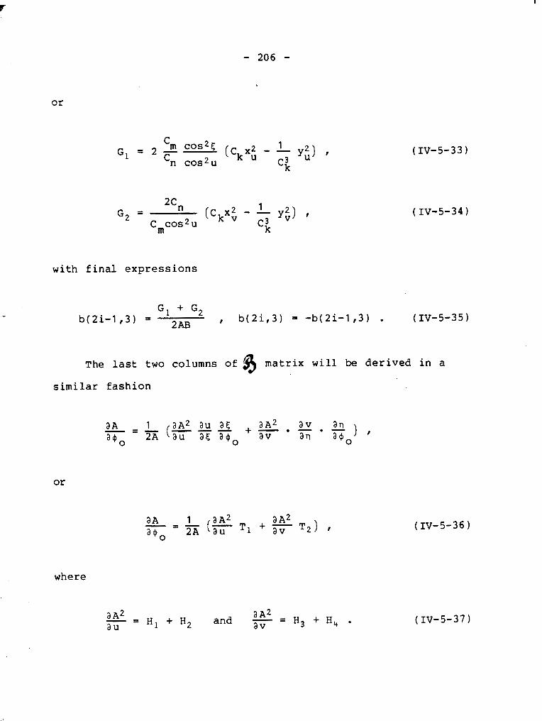
with f i n a l e x p r e s s i o n s
The l a s t t w o columns o f $ matrix w i l l be der ived i n a
s i m i l a r fa sh ion
where
a A 2 - - a A2 av - H j + H q . - H , + H ~ and - - a u

au a < L m T~ = E q = - cos u ( c o s + , s i n + - s i n 4 cosm C O S ( A ~ - A ) ) ,
0
a 2 2 H~ = - ( ) = 'n (K5 + 2K2 t a n u) , a u c o s 2 u Cm C O S ~ U
T h u s , e q u a t i o n ( IV-5-36) becomes
a n d s i n c e - a*2 = - 0 B 2 , where Xi is an a r b i t r a r y v a r i a b l e , axi ax i

For the last column of 8 matrix
where
au aa C - m U , - F . q = - - COS u cosa cosm sin(\,-A)
and
av an u2 = - - Cn sinn c o s ~ (cot (AO-A) - sinmo tann). (IV-5-48) a~ a x o
The main optimization computer program for equiareal
modified map projections was identical to all optimized mapping
systems. The differences between various projections were
given at the end of the program in subroutines in which partial
derivatives xuf yur xvr yvf x uvr Y ~ ~ f X ~ ~ f Yuuf x vvf %v were
defined.

I
The author optimized four modified equiareal map
projections:
a) Sanson's projection,
b) Mollweide's projection,
c) Hammer's projection, and
d) Eckert's IV projection.
The partial differentiation of transformation equations for
individual projections is given in the Appendix 111. The
inclusion of differential formulae in this section would make
an already difficult section completely unreadable. - - -
-
6. OPTIMIZATION RESULTS OF CONICAL PROJECTIONS
The official version of the normal aspect of the Lambert
conformal conic projection with standard parallels at latitudes
of 49' and 77' yielded the Airy-Kavraiskii measure of quality
(11-6-10) of
The first optimization dealt with the normal aspect of the
Lambert conformal conic projection. The constants of the
projection, cl and c2, were optimized. In other words,
indirectly a better choice of standard parallels was made. The
improvement resulted in a 30 percent smaller measure of
distortion. Further optimization of the metagraticule gave
even better results. The final measure of distortion was

reduced by more than one half. The Lambert equiareal conic
projection gave a slightly better result of optimization than
the conformal projection, but the smallest measure of distor-
tion was achieved with the optimized equidistant projection.
Although the position of the metapole was expected to be
identical in all optimized conic projections the author
obtained small differences which are probably caused by
numerical evaluation of linearized mathematical models.
At the suggestion of Dr. T. Poiker the author has also
determined the optimized Lambert conformal projection where the
weights were based on the distribution of population. Since
the density of population drastically varies from one side of
the country to the other, the initial approximations for
unknown parameters were difficult to determine. After many
hours of pure trial-and-error attempts, convergence of the
optimization process was finally established leading to a
reasonably good mapping system.
The optimization of cylindric and azimuthal projections
was a more stable process than the optimization of conic
projections. Convergence was easy to establish.
The results of the optimization process are given in the
following table.

CONIC PROJECTIONS:
- -
PROJECTION:
Lambert Conformal Conic (official projection)
Lambert Conformal Conic ( optimized normal)
Lambert Conformal Conic (weights: population)
Lambert Conformal Conic ( optimized) - ---
Equiareal Conic
Equidistant Conic
Table IV-6-1 Optimized parameters of conic projections

CYLINDRIC AND AZIMUTHAL PROJECTIONS:
Table IV-6-2 Optimized parameters of cylindric and azimuthal projections
"Optimized constants of Urmaev's cylindric projection are
Projection:
Mercator (Conformal Cylindric)
Equiareal Cylindric
Urmaev's Cylindric*
S tereographic
Thus, the optimized version of Urmaev's projection is almost an equidistant cylindric projection. When the values of
c
.9904
.9904
.9904
1.9678
- - coefficients a and a converge to zero the projection becomes a true equidiseant cylindric projection.
40
25' 57'
25' 57'
25" 57'
-
60' 15'
156' 27'
156" 27'
156' 27'
-91' 45'
i
A
E~~
.I096
.01096
.00775
.01130
I

7. OPTIMIZATION RESULTS OF MODIFIED EQUIAREAL PROJECTIONS
The optimization of modified equiareal projections was
much more susceptible to the divergence of the optimization
process than was the ease with the conical projection. The
determination of reasonable close approximations for unknown
parameters was decisive and it required many hours of tedious
trial-and-error approach. However, when the final approxima-
tions were found they led to very good results with respect to
the Airy-Kavraiskii measure of quality.
MODIFIED EQUIAREAL PROJECTIONS:
Table IV-7-1 Optimized parameters of modified equiareal projections
Projection
Sanson
Mo1lwei.de
Hammer
Eckert IV
40
25" 57'
25' 57'
25" 57'
25" 57'
61' 27'
61" 27'
61' 27'
61" 27'
'm
.9915
.9918
.9914
.9794
'n
.8770
1.0041
1 .OOOO
.9135
'k
1.0620
1 .I000
.9992
1.2320
h
E~~
.0105
.0070
.0069
.0068

8, CHEBYSHEV'S PROJECTIONS FOR CANADA
T h e o r e t i c a l a s p e c t s of Chebyshev 's p r o j e c t i o n s were
d i s c u s s e d i n t h e f o u r t h c h a p t e r . S e v e r a l of t h e p o s s i b l e ways
to s a t i s f y t h e fundamental r equ i r emen t of t h e c o n s t a n t s c a l e
f a c t o r a long t h e boundary polygon were d e s c r i b e d i n d e t a i l ,
However, f o r t h e p r a c t i c a l computa t ion t h e a u t h o r has d e c i d e d
t o use a series of harmonic po lynomia l s (1-7-27) on ly . The
boundary of Canadian t e r r i t o r y was approximated by 31 d i s c r e t e
p o i n t s (See F i g u r e IV-1-1). The o p t i m i z a t i o n p r o c e s s
de te rmined t h e c o e f f i c i e n t s of t h e harmonic po lynomia l s by
s a t i s f y i n g t h e fundamental c o n d i t i o n of l e a s t s q u a r e s (111-4-2)
n 1 ( I n m i ) 2 = min ,
i = l
where n extended t o a l l 31 boundary p o i n t s , S i n c e t h e number
o f unknowns is 2k + 1 , where k is t h e o r d e r of t h e harmonic
polynomial it is obv ious t h a t i n t h e c a s e of 31 boundary p o i n t s
w e can go up t o t h e o r d e r of 15 f o r t h e harmonic po lynomia l .
I n t h a t c a s e t h e boundary i s o c o l w i l l p a s s th rough a l l 31
p o i n t s . However t h e h i g h e r t h e o r d e r of t h e i n t e r p o l a t i n g
polynomia l t h e l a r g e r t h e system of e q u a t i o n s we have t o s o l v e
f o r . I t is p robab ly t h e b e s t approach t o c o n t r o l t h e sum of
t h e s q u a r e s of l o g a r i t h m s of s c a l e (IV-8-1) and i f t h e r e is no
e s s e n t i a l improvements between i - t h o r d e r and i + 1st o r d e r t o
s t o p f u r t h e r compu ta t ions . The a u t h o r has c a l c u l a t e d t h e
I
coefficients for the harmonic polynomials up to the seventh
order. The minimized sum of residuals (IV-8-1) for the seventh
order polynomial was only slightly better than the sum of the
sixth order polynomial. Thus, according to the author's
opinion, for the boundary of 31 points which define Canada,
there is no need to go further than to the sixth order. It is
naturally a questionable problem what one considers a
significant improvement and what is an unimportant change.
These questions were neither investigated nor answered. The
author was rather interested in the optimization process and
the inclusion of conformal mappings in that process was mxde
for the sake of completeness. The author is fully aware that
optimized conformal mappings have rather a small chance of ever
being used in geographic mappings. Equiareal and particularly
equidistant projections are much more applicable.

Table IV-8-1 Coefficients of harmonic polynomials

I
9. CONCLUSIONS AND RECOMMENDATIONS
This study of optimization of cartographic projections for
small scale mappings was conducted to investigate the general
approaches for obtaining the best projections using the Airy-
Kavraiskii measure of quality and, in particular, to derive the
coefficients for various mapping systems for Canadian
territory. The philosophical question whether the Airy-
Kavraiskii or the Jordan-Kavaraiskii criterion should be used
as the basis of the optimization process was answered by the
author's subjective choice of the former. The two criteria
should lead to similar results but the application of the Airy-
Kavraiskii criterion in the computation process was much
simpler. This was the main reason for its selection as the
basis of finding the best projections for Canada.
For the sake of completeness the author has added to the
research the determination of Chebyshev's projections, i.e. the
best conformal mappings, although conformal projections,
generally, should not be used for small scale maps in geog-
raphy. From the class of all analytic functions the author
optimized the complex polynomials only.
The optimization results clearly indicate that in the
family of conical projections neither conformal nor equiareal
mappings belong to the best system. The equidistant oblique
conic projection gave the best result and since it is a very
simple projection the author highly recommends its application

for small scale maps of Canada. Here we have all necessary
formulae and coefficients which fully define the recommended
projection, namely
sin 5 = sin ( sin ( + cos mo cos ( cos (Ao-A) , 0
cos ( sin (Ao-A) tan q =
sin ( cos (o - sin (o cos mo cos ( A ~ - A ) '
x = p siny , y = C 2 - p cosy .
Since the above equations for the rectangular Cartesian
coordinates ( x , y ) are related to the mapping of a unit sphere
the results of the last two equations must be multiplied by an
average radius for Canada in the scale of mapping.
The optimized versions of modified equiareal projections
also gave very good results but they are not recommended since
the three best projections: Mollweide, Hammer, and Eckert IV
involve a numerical solution of a transcendental equation for
each mapping point. Because these solutions can only be made
by a suitable iterative numerical approach, the computation
process becomes too lengthy and complicated. However, when the
equiareal property is of special importance and the cost of
computat ion is unimpor tan t then any of t h e l a s t three mod i f i ed
e q u i a r e a l p r o j e c t i o n s can be used.
Canada, t h e Uni ted S t a t e s of America and Mexico w i l l
l e g i s l a t e t h e new g e o d e t i c datum i n t h e next few y e a r s . One of
t h e r e s u l t s of t h e new North America Datum w i l l be changes to
l a r g e s c a l e mappings. Almost a l l f rames of t h e p r e s e n t l a r g e
s c a l e t o p o g r a p h i c maps of Canada w i l l have t o be changed.
Although sma l l s c a l e a t l a s maps w i l l no t be e f f e c t e d by t h e
change of datum it might be oppor tune , whi le u n d e r t a k i n g t h e s e
l a r g e m o d i f i c a t i o n s and t r a n s f o r m a t i o n s , f o r g e o g r a p h e r s t o
select a b e t t e r c a r t o g r a p h i c system. The system sugges t ed by
t h e a u t h o r has s e v e r a l recommendations.
EPILOGUE, WRITTEN BY LEWIS CARROLL
"What 's t h e good of M e r c a t o r ' s Nor th P o l e s and Equa to r s ,
T r o p i c s , Zones, and Mer id ian Lines?" So t h e Bellman would c ry : and t h e crew
would r e p l y "They a r e mere ly c o n v e n t i o n a l s i g n s ! O the r maps a r e such shapes , wi th t h e i r
i s l a n d s and capes! But we've g o t our brave C a p t a i n t o thank"
( S o t h e crew would p r o t e s t ) " t h a t h e ' s bought us
THE BEST - A PERFECT AND ABSOLUTE BLANK!"
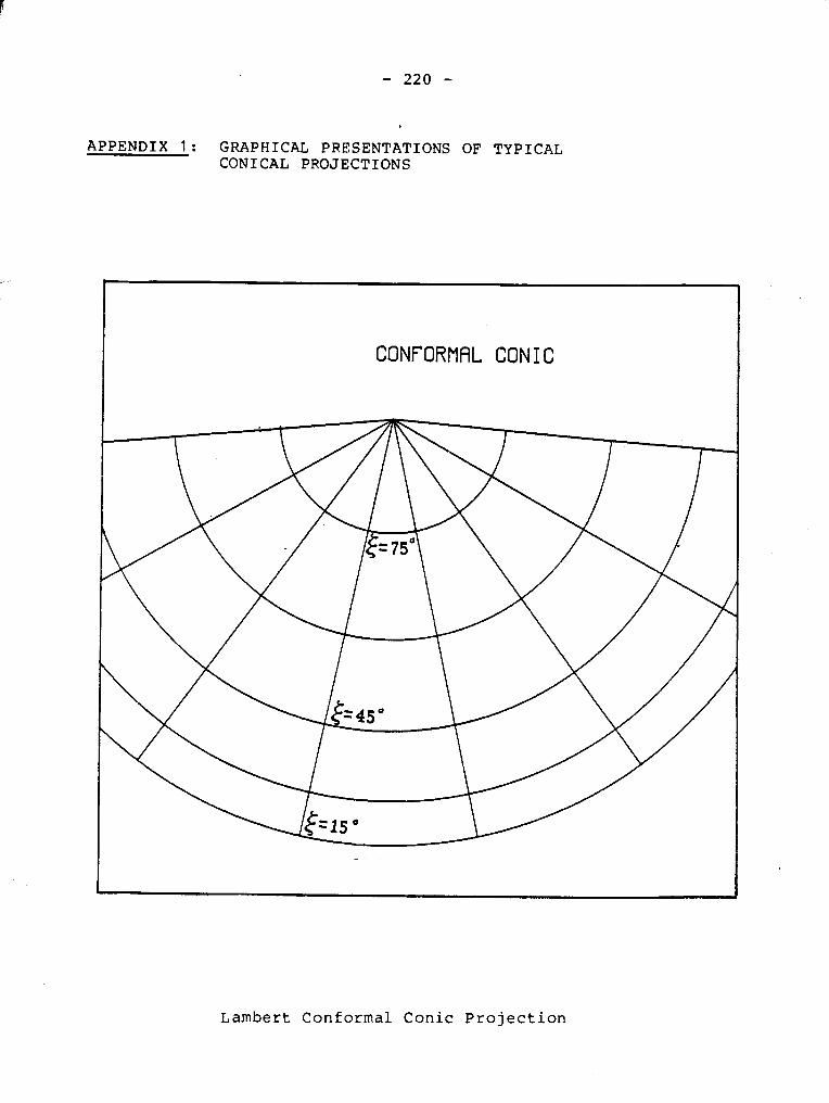
APPENDIX 1: GRAPHICAL PRESENTATIONS OF TYPICAL CONICAL PROJECTIONS
CONFORMRL CONIC
Lambert Conformal Conic Projection

STEREOGRAPHIC PROJECTION
I
Oblique Aspect of Stereographic Projection

MERCATOR PROJECTION
Mercator Projection

Equidistant Cylindric Projection

APPENDIX 2: GRAPHICAL REPRESENTATION OF TYPICAL EQUIAREAL MODIFIED PROJECTIONS
Sanson's Projection
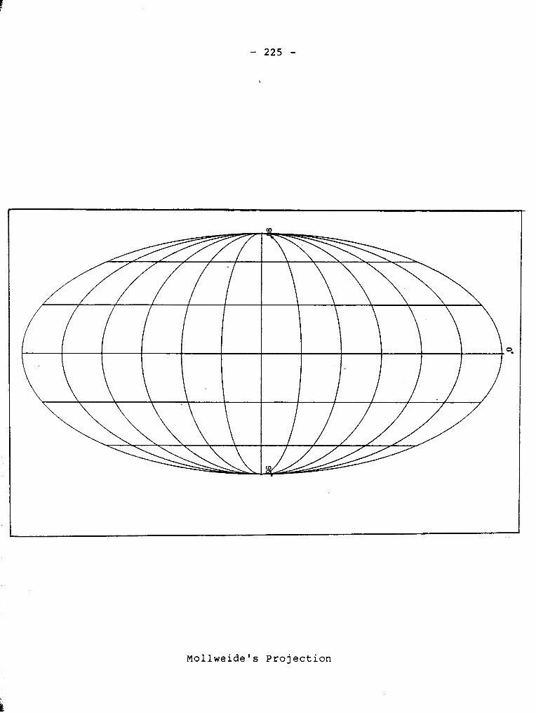
Mollweide's Projection
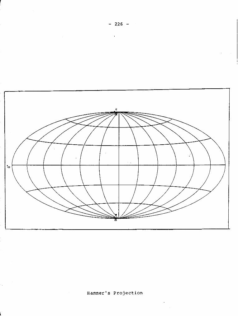
Hammer's Projection

APPENDIX 3: DERIVATION OF FORMULAE FOR OPTIMIZED MODIFIED PROJECTIONS
(i) Sanson's Projection:
v sin u , x = cos u v
x = - uv sin u
x = - v COS u , uu Yuu = 0
(ii) Mollweide's Projection:
2$ + s i n 2 J, = n sin u

Computation of $:
TI $(O) =, sin u for i = 0 to n
F'(i) = 2(1 + cos 2$)
The iterative process is repeated until two successive
iterations are practically identical, i.e.
I$(i+l) - $(i) I < E ,
where E is an arbitrarily selected small number.
& = r r COS u du 2 1 + cos 214
2 4 5 x = - u TI
v sin $
2JZ Xv = -
TI cos $
x = - ' I2 sin + TI
9 u l v du
- uu - 2 J r v ll
(($12 cos q + sin + a) du2

( C O S
71
w h e r e
s i n
s i n s i n
( i i i ) H a m m e r ' s Projection:
v
X = 2 cos u s i n 7 , = s i n u 6
COS - 6 2 cos 7
v COS 6 = COS u COS - 2 '
- v s i n u d 6 = COS - d u 2 s i n 6 '
d 6 d 2 6 s i n 6 cos u - s i n u cos 6 - - = v
cOs 2 d u t
d u 2 s i n 2 6

d26 - = cos u 1 v v d6 (7 s i n 64 cos 7 - s i n 7 cos 6 -) , dv2 2 s i n 2 6 dv
d26 = - - 1 v v d6 du dv
s in (7 s i n 6 s i n 7 + cos 6 cos 7 a;) , s i n 2 6
v s i n 7 X = 6 d6 6
6 (cos u s i n - - - 2 s i n u c o s 7) , U cos2 7 2 du
- - cos u 6 v 6 v d6 Xv 6 ( C O S 7 cos 7 + s i n - s i n 7 =) ,
cos2 7 2
1 x = - 6 1 v 6 d6 6 uv 6 ( c o s ~ ~ ( ~ C O S ~ ( C O S u s i n - - - 2 s i n u cos 7) +
cos4- 2 du 2
v 1 6 d26 6 d6 d6 + s i n - - + + s i n 7 ( c o s u (7 c o s - - - 2 du dv 2 du dv
+ s i n u s i n 6 d6 7 a ; ) ) +
1 v 6 d6 6 d6 + s i n 6 - s in - - (cos u s i n - - - 2 s i n u cos- - 2 2 2 du 2)dv)

v s i n 2 x = - 6 1 6 d S 2 +
6 d6 * C o s U cos T(x) ( c 0 s 2 ~ ( - s i n u s i n - -
uu cos4- 2 du 2 2
6 d 2 6 6 6 d6 + cos u si? - - 2 con u COST + s i n u s i 5 =) + du2
1 6 d6 5 d6 + 5 ( c o s u s i n - - - 2 s i n u cos I ) s i n 6 =) 2 d u
cos u 6 6 v d6 2 6 v X = vv 6 ( C O S ~ 7 (COST s i n (=) - COST s i n - +
2 C O S ~ I 2
6 v d 2 6 + 2 s i n I s i n - -) t dv2
d6 6 v 6 v d6 + s i n 6 ( c o s 2 cos + s i n 7 s i n T ~ ) ) ,
- 1 6 1 ( c o s 7 cos u + - s i n u s i n 6 d6 Yu - 6 2 T Z ) c o s 2 3
6 d6 s i n u s i n - - - 2 d v Yv - 6 2 cos 2 7
- 1 6 1 6 d6 d6 ( c 0 s 2 ~ ( 7 s i n u COT ;i;-;i; - 6 %v - 6
d 6 + s i n ? cos - d v 2 C O S ~
6 d26 d6 6 1 6 d6 + s i n u sixy m ) + s i n 6 - ( c o s ~ c o s u ~ s i n u d v sixy =)) ,

- - 1 ( c o s 2 q 6 (T 1 6 6 s i n u cosd d6)2- 2 c o s q s i n u +
Yuu 2 c o s 4 ~ 2 ( d u i
6 d 2 6 d6 6 1 6 d6 + s i n u s i 3 - ) + s i n & - ( c o s ~ c o s u + l s i n u s i ~ x)) , d u2 d u
- - 6 1 6 d6 6 d26 s in (cos21 (- cos- (-1 + s i n - - + Yvv 6 2 C O S ~ \ 2 2 d u d v 2
6 d6 2 + s i n u s i n 6 s i n 2 (=) ) .
( i v ) E c k e r t ' s I V P r o j e c t i o n :
X = 2 2 G v ( 1 + cos 'f ') , y = - s i n 'f' rn m
C o m p u t a t i o n of 'f':
1 Y ( O ) = 7 ( I + i) s i n u ,
1 ~ ( i ) = 'f'(i) + 2 s i n Y ( i ) + T s i n 2 Y ( i ) - ( 2 + $ ) s i n u ,
F 1 ( i ) = 1 + 2 cos Y ( i ) + cos 2 ~ ( i )
for i = l t o n

u n t i l
'II
dY ( 2 + ?) cos u - = I
d u 1 + 2 cos w + cos 2Y
ll
d2 Y 2 + T - = d Y ( s i n y + s i n 2 ~ ) - ( 2 cos u ,, du2 ( 1 + 2 cosy + cos 2 ~ ) ~
- s i n u ( 1 + 2 cos Y + cos 2 1 ) ) ,
= - 2 d~ v s i n Y , rn
Xuv = - 2 dY s i n Y a; , rn
x = - 2v dlu 2 d 2 ~ ( c o s y (z) + s i n Y -) , uu m T T T d u2
2 G = - dY cos Y , Yu 6
2 G = - d 2 ~ dY 2
yuu ( C O S Y - - s i n Y ) . rn d u2
BIBLIOGRAPHY
Adler, K.H.; Reilly, J.P.; Schwarz, C.R. 1968. A generalized system for the evaluation and automatic plotting of map projections. Canadian Surveyor, 22, No. 5, pp. 442-450.
Airy, G.B. 1861. Explanation of a projection by balance of errors for maps applying to a very large extent of the earth's surface; and comparison with other projections. Philosophical Magazine and Journal of Science, Vol. 22, pp. 409-421.
Biernacki, F. 1965. Theory of Representation of Surfaces for Surveyors and Cartographers. U.S. Department of Commerce and the National Science Foundation, Washington, D.C.
Biernacki, F. 1973. Podstawy Teorii Odwzorowan Kartograficznych. Panstwowe Wydawnictwo Naukowe, Warsawa (Polish). - -.- .-
~orzi6, B. 1955. ~atematizka Kartografija. ~echniEka Knj iga, Zagreb, (Croatian).
Chovitz, B.H. 1952. Classification of map projections in terms of the metric tensor to the second order. Bollettino di Geodesia e Scienze Affini, Vol. 1 1 , No. 4, pp. 379-394.
Chovitz, B.H. 1954. Some applications of the classification of map projections in terms of the metric tensor to the second order. Bollettino di Geodesia e Scienze Affini, Vol. 13, No. 1, pp. 47-67.
Chovitz, B.H. 1977. Perspective projections in terms of the metric tensor to the second order. (unpublished - personal correspondence)
Clarke, A.R. 1879. Mathematical geography. Encyclopaedia ~ritannica, (9-th edition), Vol. X, p. 204, Edinburg.
Colvocoresses, A.P. 1965. A Unified Plane Coordinate Reference System. Dissertation, The Ohio State University.
Conte, S.D.; Carl de Boor. 1972. Elementary Numerical Analysis. McGraw-Hill Book Company, New York.
Courant, R.; Hilbert, D. 1937. Methoden der mathematischen Physik 11. Springer Verlag, Berlin, (German).

Deetz, C.H.; Adams, O.S. 1945. Elements of Map Projections. U.S. Department of Commerce, Coast and Geodetic Survey.
Special Publication No. 68, Washington D.C.
Dennis, J .E. 1977. Non-linear Least Squares and Equations. The State of the Art in Numerical Analysis. Academic Press, New York.
Driencourt et Laborde. 1932. Traite des projections des cartes geographiques a llusage des cartographes et des geodesiens. Hermann et C-ie, Paris, (French).
Ecker, E. 1978. Conformal mappings of the earth ellipsoid. Manuscripta Geodaetica, Vol. 3, pp. 229-251.
Eisenhart, L.P. 1960. A Treatise on the Differential Geometry of Curves and Surfaces. Dover Publication, New York.
Fiala, F. 1957. Mathematische Kartographie. VEB Verlag Technik, Berlin., (German) . Fischer, E.U. 1979. Zur Transformation digitaler kartographischer Daten mit Potenzreihen. Nachrichten aus dem Karten-und Vermessungswesen. Verlag des Instituts fur angewandte ~eodasie, Frankfurt, (German).
v Francula, N. 1971. Die vorteilhaftesten Abbildungen in der Atlaskartographie. Institut fzr Kartographie und Topographie der Universitat Bonn, Bonn, (German) . ~ranzula, N. 1974. Izbor Projekcije. Geodetski Fakultet ~veuEiligta u Zagrebu, Zagreb, (Croatian).
Frankich, K. 1977. Mathematical Cartography. Lecture Notes, British Columbia Institute of Technology, Burnaby, B.C.
Frankich, K. 1977. A Study in Conformal Mappinq. University of New Brunswick, Technical Report No. 45, Fredericton, N.B.
Frolov, Y.S. 1968. A general index of map projection distortions. Geodesy and Aerophotography, pp. 333-335, American Geophysical Union, Washington, D .C.

,
Gauss, C.F. 1825. Allgemeine ~uflasung der Aufgabe die Theile einer gegebenen lac he auf einer anderen gegebenen lac he so auszubilden dass die Abbildung dem Abgebildeten in den kleinsten Theilen Shnlich wird. Astronomische Abhandlungen, Vol. 3, pp., Altona, (German).
Gilbert, E.N. 1974. Distortion in maps. SIAM Review, Vol. 16, pp. 42-67.
Ginzburg, G.A. 1936. Novie azimutalnije projekcii. Geodezist, No. 2, pp. 43-50, (Russian).
Goetz, A. 1970. Introduction to Differential Geometry. Addison Wesley Publishing Company, New York.
Goussinsky, B. 1951. On the classifications of map projections. Empire Survey Review, No. 7, pp. 75-79.
Graur, A.V. 1956. Mathematical Cartography. Geo-Sciences Branch, Chart Research Division, Aeronautical Chart and Information Center, St. Louis 18, Mo.
Grieve, M. 1949. Memorandum to Mr. M.G. Cameron. Department of Energy, Mines and Resources Archive.
Grossmann, W. 1976. ~eodatische Rechnunqen und Abbildungen in der Landesvermessunq. Verlaq Konrad Wittwer, Stuttgart, (German) . Hojovec, V. 1977. La classe des projections equidistantes dans les meridiens et dans les parallels. Studia Geophisica et Geodaetica, Vol. 21, pp. 118-126, (French).
Heissler, V.; Hake, G. 1970. Kartographie. Walter de Gruyten and Company, Berlin, (German).
Heuvelink, H.J. 1918. De stereografische kartenprojectie in hare toepassing. Nederlandische Rijksdriehoeksmeting, (Dutch).
Hinks, A.R. 1912. Map Projections. University Press, Cambridge.
Hoschek, J. 1969. Mathematische Grundlaqen der Kartoqraphie. Bibliographisches Institut, Mannheim, (German).

Hotine, M. 1946. The orthomorphic projection of the spheroid, Empire Survey Review, Vol. 8 : pp. 300-31 1 , Vol. 9 : pp. 25-53, 52-70, 112-123, 157-166.
Hristow, W.K. 1955. Die Gausschen und geographischen Koordinaten auf dem Ellipsoid von Krassowsky. VEB Verlag Technik, Berlin, (German) . Jordan; Eggert; Kneissl. 1958. Mathematische ~eodasie, Handbuch der Vermessunqskunde, Vol. 4, 10-th edition, Metzlersche Verlagsbuchh., Stuttgart, (German).
Kantorovich, L.V.; Krylov, V.I. 1958. Approximate Methods of Higher Analysis. P. Noordhoff Ltd., Groningen.
Kavraiskii, V.V. 1959. Izabranie Trudi, Vol. I, 11, 111, Matematicheskaya Kartografiya. Hyrographic Service VMF, Moscow, (Russian). - - - - ----.
Koning, R.; Weise, K.H. 1951. Mathematische Grundlagen der hoheren ~eodasie und Kartographie. Springer Verlag, Berlin, (German).
Krakiwsky, E.J. 1973. Conformal Map Projecti-ons in Geodesy. Lecture Notes No. 37, Department of Surveying Engineering, University of New Brunswick, Fredericton, N.B.
Lagrange, J .L. 1884. ~ b e r Kartenprojection. Ostwalds Klassiker der exacten Wissenschaften, No. 55, Leipzig, (German).
Lambert, J.H. 1972. Notes and Comments on the Composition of Terrestrial and Celestial Maps. Michigan Geographical Publication No. 8, Department of Geography, University of Michigan, Ann Arbor.
Lee, L.P. 1943. The nomenclature and classification of map projections. Empire Survey Review, No. 7, pp, 190-200.
Lee, L.P. 1953. A Transverse Mercator Projection of the spheroid alternative to the Gauss-Kruger form. Empire Survey Review, Vol. 12, pp. 12-17.
Lee, L.P. 1961. The Transverse Mercator Projection of the entire spheroid. Empire Survey Review, Vol. 16, pp. 208-217.

Lee, L.P. 1974. The computation of conformal projections. Survey Review, Vol. 22, No. 172, pp. 245-256.
Lee, L.P. 1976. Conformal Projections Based on Elliptic Functions. Cartographica, Monograph No. 16, York University,
--
Toronto.
Maling, D.H. 1959-1960. A review of some Russian map projections. Empire Survey Review, Vol. 15, pp. 203-215, 255-266, 294-303.
Maling, D.H. 1973. Coordinate Systems and Map Projections. George Philip and Son ~td., London.
Meshcheryakov, G.A. 1968. Teoreticheskie osnovi matematicheskoy kartografii. Nedra, Moscow, (Russian).
Mikhail, E.M. 1976. Observations and Least Squares. IEP-A Dun-Donnelley Publisher, New York.
Miller, O.M. 1942. Notes on cylindrical world map projections. Geographical Review, Vol. 32, pp. 424-430.
Milnor, J. 1969. A problem in cartography. The American Mathematical Monthly, No. 10, pp. 1101-1112.
Moritz, H.; Sunkel, H. 1978. Approximation Methods in Geodesy. Herbert Wiechmann Verlag, Karlsruhe.
Pavlov, A.A. 1959. 0 terminologii v matematicheskoy kartografii. Geograficheskiy Sbornik, Vol. XIII, Academy of Science of USSR, Moscow, (Russian).
Pavlov, A.A. 1964. Obzor klasifikacii kartograficheskih projekcii. Vestnik Leningradskogo Universiteta, No. 24, pp. 145-153, (Russian).
Pavlov, A.A. 1974. Prakticheskoe Posobie po Matematicheskoy Kartografii. Publication of University of Leningrad, Leningrad, (Russian) . Peters, F.H. 1945. Memorandum to Mr. Murdie, Department Energy, Mines and Resources Archive.

Peucker, T.K. 1972. Computer Cartography, Commission on College Geography, Resource Paper No. 17. Association of American ~eogra~hers, washington, D .C.
Rectorys, K. 1977. Variational Methods in Mathematics, Science and Engineering. D. Reidel Publishing Company, Boston.
Reilly, W.I. 1973. A conformal mapping projection with minimum scale error. Survey Review, Vol. 22, No. 168, pp. 57-71.
Richardus, P.; Adler, R.K. 1972. Map Projections. American Elsevier Publishing Company, New York.
Robinson, A.H. 1951. The use of deformational data in evaluation world map projections. Annals of the Association of American Geographers, Vol. 41, No. 1, pp. 58-74.
Robinson, A.H. 1974. A new map projection: its developments and characteristics. International Yearbook of Cartography, Vol. 14, pp. 145-154.
Sebert, L.M. 1970. The history of the 1 :25OOOO map of Canada. The Canadian Cartoqrapher, Vol. 7, No. 1 , pp. 15-26.
Siemon, K. 1938. ~lachenproportion~lls Umbeziffern der Punkte in ~artenentwurfen. Mitteilung des Reichsamts fcr Landesaufnahme, No. 14, pp. 34-41, Berlin, (German).
Sigl, R. 1977. Ebene und spharische Trigonometrie. Herbert Wichmann Verlag, Karlsruhe, (German).
Snyder, J.P. 1977. A comparison of pseudocylindric map projections. The American Cartographer, Vol. 4, No. 1, pp. 59-81.
Solovev, M.D. 1969. Matematicheskaya Kartografiya. Nedra, Moscow, (Russian).
Taschner, R.J. 1977. Differentialgeometrie fcr ~eodzten. Manz Verlag, Vienna, (German).
Thomas, P.D. 1952. Conformal Projections in Geodesy and Cartography. U.S. Coast and Geodetic Survey, Special Publication No. 251, Washington, D.C.

Tobler, W.R. 1961. Map Transformation of Geographic Space. ph.D. dissertation, University of Washington.
Tobler, W.R. 1962. A classification of map projections. Association of American Geographers, Vol. 52, No. 1, pp. 167-175.
Tobler, W.R. 1963. Geographic area and map projections. - The Geoqraphical Review, Vol. 53, No. 1 , pp. 59-78.
Tobler, W.R. 1964. Some new equal area map projections. Empire Survey Review, pp. 240-243.
Tobler, W.R. 1973. The Hyperelliptical and other new pseudo cylindrical equal area map projections. Journal of Geophysical Research, Vol. 78, No. 1 1 , pp. 1753-1759.
Tobler, W.R. 1974. Local map projections. The American Cartographer, Vol. 1, No. 1 , pp. 51-62.
Tobler, W.R. 1977. Numerical approaches to map projections. Festschrift Arnberger, Kretschmer, Vienna.
Tobler, W.R. 1979. Smooth Pycnophylactic Interpolation for Geographical Regions. ~ournai of- the American statistical Association, Vol. 74, Number 367, pp. 519-535.
Urmaev, N.A. 1953. Isledovania po matematicheskoy kartografii. Publication of CNIIGAIK, NO. 144, Moscow, (Russian).
Vahramaeva, L .A. 1963. Generalized formulas for conformal projections.
Wagner, K. 1941. Neue okumenische ~etzenentwiirfe fbr die kartographische Praxis. Jahrbuch der Kartographie, Bibliographisches Instit, Leipzig, pp. 276-202, (German) . Wagner, K. 1962. Kartographische Netzenetwurfe, Bibliographisches Institut, Mannheim, (German).
Weber, H. 1867. iber ein Prinzip der Abbildung der teile der ~rdoberflache. Journal fbr Mathematik, 67, p. 229.

Wilski, V.I. 1978. Ein Program zum Entwerfen und Zeichen geographischer Netz. Nachrichten aus dem Karten-und Vermessungswesen, Verlag des Instituts fiir angewandte Geodasie, Frankfurt, (German) . Wray, T. 1974. The seven aspects of a general map projection. Cartographica, Monograph No. 1 1 , York University, Toronto.
Wray, T. 1974. An plane coordinates. pp. 637-642.
Young, A.E. 1920. Projections. Royal
integrated approach to map projections and The Canadian Surveyor, Vol. 28, No. 5,
Some Investigations in the Theory of Map Geographic Society, London.