Computers ind. Engng Vol. 18, No. 1, pp. 95-103, 1990 0360-8352/90 $3.00 + 0.00 Printed in Great Britain. All rights reserved Copyright © 1990 Pergamon Press plc

O P T I M I Z A T I O N O F M U L T I V A R I A T E S I M U L A T I O N O U T P U T M O D E L S U S I N G A G R O U P S C R E E N I N G

M E T H O D

JEFFERY K. COCHRAN a n d JINNCHYUN CHANG

Systems Simulation Laboratory, Department of Industrial & Management Systems Engineering, Arizona State University, Tempe, AZ 85287, U.S.A.

(Received for publication 20 April 1989)

Abstract--Computer simulation is often used to identify the set of model variable values which appear to lead to optimal performance of the modeled system. When all variables are quantitative, experimental designs and procedures known as response surface methodology (RSM) can be used in dealing with this optimization problem. Previous research has emphasized the situation in which there are only two independent variables. If there are more than two independent variables, it becomes difficult to find optimization and the simulation processes may be expensive. Nevertheless, these are common circum- stances. This paper proposes a methodology using a two-stage group screening experimental design to investigate which subset of the variables is most important in explaining the optimum response variable. A simulation of a new generation of flight simulator is analyzed to determine the values of six variables that will optimize the values of a dependent variable simultaneously. The group screening technique is a powerful and robust tool to implement response surface methodology strategies.

INTRODUCTION

A computer simulation is an experiment in which input variables are statistically combined to produce a dependent variable or response. Simulation may be defined as the technique of constructing and executing a computer model of an abstraction of a real world system to attempt to measure and improve, by design, that system [1]. Therefore, the response from the simulation model is dependent on its input variables. Every response is the combination of different input variables. Analysts are interested in finding the optimal combination of those input variables or in investigating the relationship between the response and the input variables. When finding the optimal response, inefficient computer runs can be avoided [2]. Response surface methodology (RSM) efficiently reduces the number of simulation runs while fulfilling the analyst's objectives. In using response surface methodology, the results of different simulation runs build the "response surface," and a search method is used to look for the optimum (if it exists).

Unfortunately, the literature of RSM deals almost exclusively with cases in which the model is reported to contain only one or two input variables. In reality most simulation models involve more than two input variables. The difficulty in having more than two input variables is that more simulation runs are needed to get the same statistical significance in the response surface contours. This paper presents a methodology that seeks the optimum response value for a multivariable computer simulation model at low computational expense.

Perhaps the most significant early work in the development of response surface methodology was done by Myers [3]. More recently, developments in RSM are collected by Biles [4] and by Khuri and Cornell [5]. Smith [6] surveys a number of search techniques for seeking the optimum solution based on response surface contours. Because such a search is often a trial-and-error process, many time-consuming calculations are involved. Therefore Smith [7] developed a computer program which conducts an automatic search for optimum solutions. Safizadeh and Thornton [8] have used an example of inventory control to also demonstrate the usefulness of RSM.

Smith and Mauro [9] found that only a few input variables have a significant effect on the response in many simulation models. They suggest using the group screening method which was first introduced by Watson [10] to identify those significant variables. Kleijnen [11] also advocates the use of group screening (GS) to detect the few factors which have major effects in the response, and are essential when simulation models have too many input variables. To conduct a screening experiment, Mauro and Smith [12] suggest using the two-stage group screening.

CArE ~8/~-q3 95

96 JEFFERY K. COCHRAN and J1NNCHYUN CHANG

The Group Screening and Response Surface methodology is presented in Fig. 1. At the beginning of the search for the optimum solution, a simulation model may have many input variables (k)~ Frequently, only a few variables have significant effects on output. The two-stage group screening method is first used to find those major variables. After group screening, our method considers only significant variables. Those variables are then used in RSM to find the optimal solution.

The first part of this paper states the group screening method, and then gives a brief overview of how the group screening method works. The second part of this paper briefly discusses RSM methodology. Finally, the use of experimental design to establish response contours, and the use of first order polynomial and second polynomial searches necessary for finding optimum solutions are presented. To more thoroughly illustrate the procedures for using group screening and RSM methods, an example of a simulation model which describes a new-generation flight simulator is used. The objective of that simulation output analysis is to find the best combination of input variables that would minimize the number of object pictures that do not appear on the screen.

GROUP SCREENING OVERVIEW

Suppose a simulation model has n controllable input variables, and at least one output variable from the model (which can be called the response of the combination of input variables). The mathematical relationship between those input variables and the response is unknown and may be represented as:

Y = F(X,, )(2 . . . . . X , ) + e.

Here, F is a mathematical function of n input variables that determines the values of the response Y, and e is an error term where E(e~) = 0 and Var(e~) = constant. The value of the true response Y is dependent on the values of each Xi variable. Because the actual mathematical function F is unknown, an approximation form using a polynomial is frequently employed to approach this real function. A linear equation is always sufficient to represent this polynomial form [13, 14]:

Yi = Bo + ~ BjXii + e~ /= I

where Y~ is the ith response and Xv is the j th input variable and ith combination. B0, B~ . . . . . B, are unknown parameters.

Some of the input variables will have a significant effect on the output of the model and some of them will not. A general factorial experimental design such as the 2 x full factorial design or the fractional factorial design may be used to investigate which factors are important in the model. If the model has 10 input factors, then the 2 K full factorial design can have 124 cells. However, one simulation run does not completely determine the distribution of the output variable. Multiple replications are needed to obtain a good statistical estimation for a cell. Consequently, there are

I Znput variables 1 X1, X2~..., Xk

111 screening methodology

Significant variabLes 1 y1, y2t,,.~yn <k Response surface methodology

Optimal soLution

Fig. 1. Methodology flowchart.

Multivariable simulation output models 97

many simulation runs for any factorial design. Therefore, group screening methodology provides potential advantages in reducing the number of simulation runs required to reach optimum,

The group screening method is based on the aggregation principle. Some prior knowledge about the simulated variables is required so that the related variables can be put into groups. If this premise cannot be satisfied, the group screening method does not produce any gains over a usual experimental design such as full factorial design.

Group screening was first introduced by Watson in 1961. He suggested that k variables in the model can be separated into g groups. Each group is regarded as a single variable [10]. In doing this, Watson made the following assumptions:

(1) All factors have, independently, the same prior probability of being effective, (2) Effective factors have the same effect, A > 0, (3) There are no interactions present, (4) The required design exists, (5) The direction of possible effects are known, (6) The errors of all observations are independently normal with constant known variances, and (7) f = gk, where g = number of groups, and k = number of factors per group.

Assumption (5) is nearly always a problem in application because the directions of some input factors are unknown. Mauro and Smith [12] demonstrated that group screening is still a method worthy of using even in the worst case in which the directions of factors are mixed up. To detect as many of the effective and noneffective factors as possible, the unclear factors should be put in one group to avoid effect cancellations.

The grouping techniques can be summarized as follows:

(1) If the direction of the factor is unknown, put this factor in one group, (2) Put the positive important factors in one group, (3) Put the factors with the same direction and possible effect in one group, and (4) Put the factors with the same direction and little effect in one group.

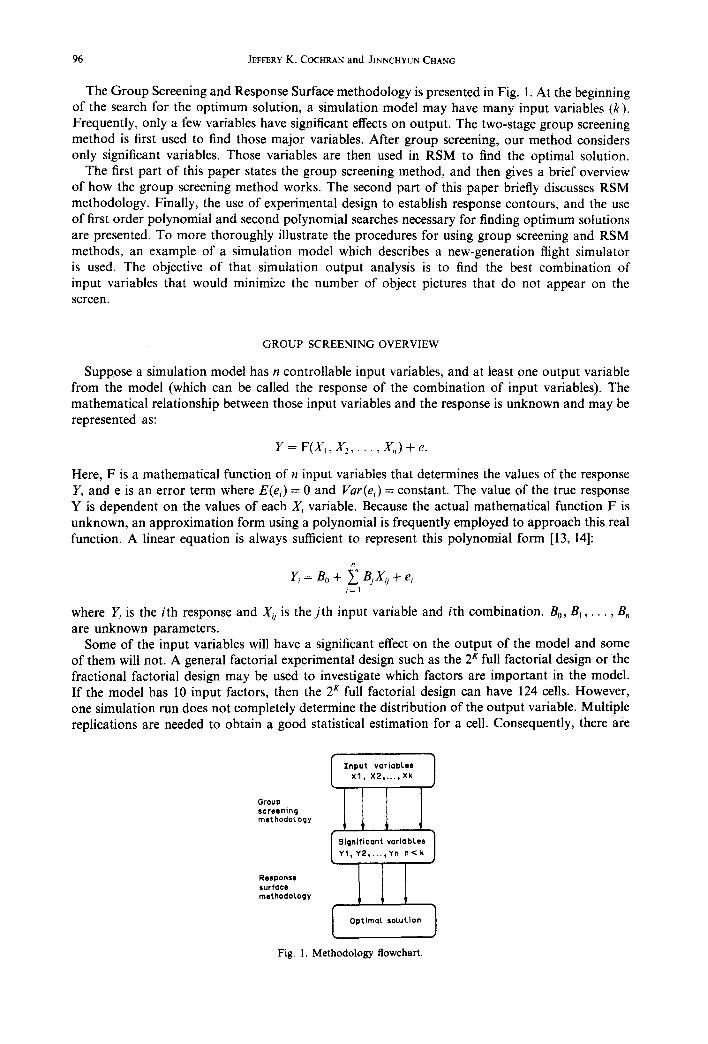
The procedure for using the group screening method is summarized in Fig. 2. After grouping factors into several groups, each group is then regarded as a single factor. In the first stage of the

Xl X2 X3 X4 X5 X6

(Znput variables)

First stage

Second stage

,o,,,- ® ® @ grouping

Experimental design

Experiment.nL design

Q

Effect 1 Effect[

@ ® (Significant groups)

Xl X2

X1

(Significant variabLes)

x3

I Effect

X3

Fig. 2. Group screening flowchart.

98 JEFFERY K. COCHRAN and JINNCHYUN CHANG

group screening, full factorial design is suggested to avoid missing any interaction between variables if there are only three or four groups. When there are more than four groups, then a 2 xp fractional factorial design is employed to reduce the number of computer runs and save time under the assumption that high-level interaction can be ignored. In the second stage of group screening, only the variables within the significant group are considered. The 2 K'p fractional factorial design or the 2 K full factorial design is used again to screen out the unimportant variables. The remaining variables are the most significant variables in the simulation model. Additional information on two-group screening may be found in [15].

REVIEW OF RESPONSE SURFACE METHODOLOGY

After two-stage group screening, suppose N input variables remain in the simulation model. The relationship of the response and input variables can now be expressed as:

Z = F ( X I . . . . . XN)+e where N < n .

The actual functional form of this relationship is generally unknown, and different combinations of Xi produce different responses. To find combinations of Xi for optimal response, a systematic method (response surface methodology) is helpful rather than a brute force search. RSM can be divided into the following steps:

(1) First-order model design, (2) Determining the optimal condition, (3) Second-order model design, and (4) Determining the optimal solution.

Each of these parts of our methodology are briefly discussed below.

First-order model design

RSM makes the assumption that the response function F can be approximated in a certain region by a low-order polynomial equation. The general form of the first-order model equation is:

Y = Bo + B I X I + " " + BNXN + e,

where

Y = response, Bi = unknown parameter, Xi = input variables, e = e r r o r term.

In finding this polynomial equation and describing how the response is influenced by the input variables, a proper experimental design saves time and expense in generating data points of the design cells. For example, a model with 2 variables can be fit by:

Y = Bo+ BIXI + BeX2 + B 3 X I X 2 .

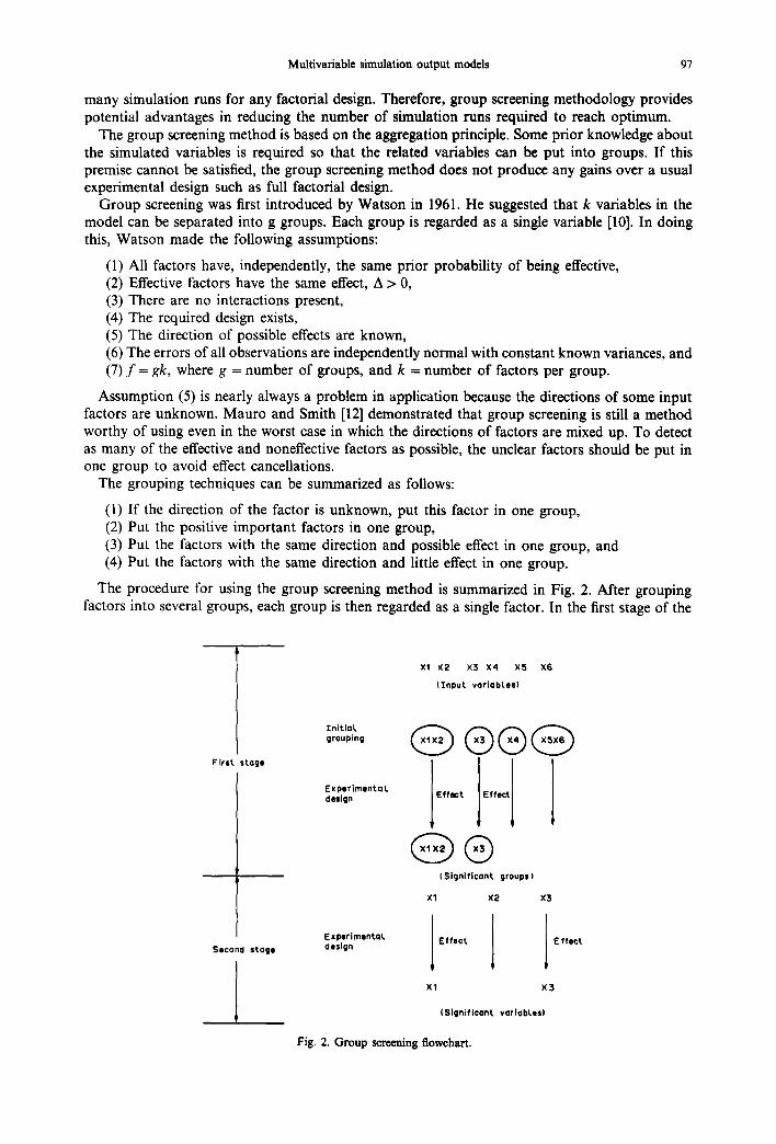
To find four unknown variables, at least four data points are required. Therefore, the 2 ~ factorial design provides more than enough data. Its design structure and graph are presented in Fig. 3.

After obtaining a first-order model equation, ANOVA analysis is used to perform a "lack-of-fit" test to determine whether the estimated equation can adequately represent a given simulation response function or not.

Determining the optimal condition

If the estimated equation of the first-order model is adequate to demonstrate the response function, the steepest ascent or the steepest descent method can be applied to search for the optimal condition. The steepest ascent and the steepest descent are methods of looking for better conditions along the steepest direction of the equation. A series of experiments is performed along the path until no further improvements appear in the response. This means that the particular equation is no longer sufficient to describe the response function in the new region. Therefore, another

Multivariable simulation output models 99

x2

Experiment point.

VaLues Xl X2

1 +1 +1

2 +1 - I

3 --1 + I

4 - 1 -1

( - 1 , +11

( - I , - 1 )

(+1, +1)

X1

(+1, --1)

Fig. 3.2 k Factorial design.

experimental design for the first-order model must be developed to find another estimated equation approaching the response surface. These searching processes continue until the first-order polynomial equation can no longer improve the response function. This condition is determined from a lack-of-fit test.

Second-order model design When the estimated first-order equation cannot describe the response surface adequately, the

search process has probably reached a stationary region or is close to the optimal area. A quadratic equation generated by the second-order experimental design may now approach the shape of the response function. The general form of the estimated second-order equation may be represented as:

K K K - I K

Y = B 0 + Z B , X , + ~ B , , X 2 + ~ ~ BuX, Xj + e. i = 1 i ~ l j = l j = 2

To save computer runs and time expense, we prefer the Central Composite Design (CCD) here. Using experimental data points, an estimated second-order equation is constructed by the regression analysis method. A fit test is used again to check whether this equation can adequately represent the response surface.

Determining the optimal solution The slope reveals the variables' rate of change with respect to the other variables in a functional

equation. The slope of a function is given by its derivative and extreme points are found by setting the derivative for the variable equal to zero. For a function with two or more variables, the partial derivative for every variable is equal to zero. That is, at the extreme point of F(X(, )(2 . . . . . XK):

OF(X(, X2 , . . . , XK) = 0 for all N = 1 , . . . , K. ~XN

When the X variables have achieved a set of values that cause all derivative equations to be zero, then F(X(, 3(2 . . . . , Xu) is an extreme point. This set of values is the answer to the simulation model optimization problem. Additional information on empirical model building and response surfaces is available in [16]. In the next section, we present an example application of our complete methodology from a recently completed research project.

EXAMPLE OF METHODOLOGY APPLICATION AND VALIDATION [17]

The following example helps to illustrate our combined GS and RSM method. Flight simulators allow pilots to obtain flying experience without using actual aircraft. The current software-driven simulators have not developed to the point where realistic computer-graphic images provide an illusion of flight. Therefore, Honeywell is developing a flight simulator device which creates an experience similar to viewing a film, where the pilot controls the field of view [18]. The equipment included in this model are storage disks, image buffers, a geometric converter, and data pipelines to the image screen. Because such equipment is very expensive, a simulation model was built to simulate alternative configurations of those devices that might meet performance requirements at

100 JEFFERY K. COCHRAN and JINNCHYUN CHANG

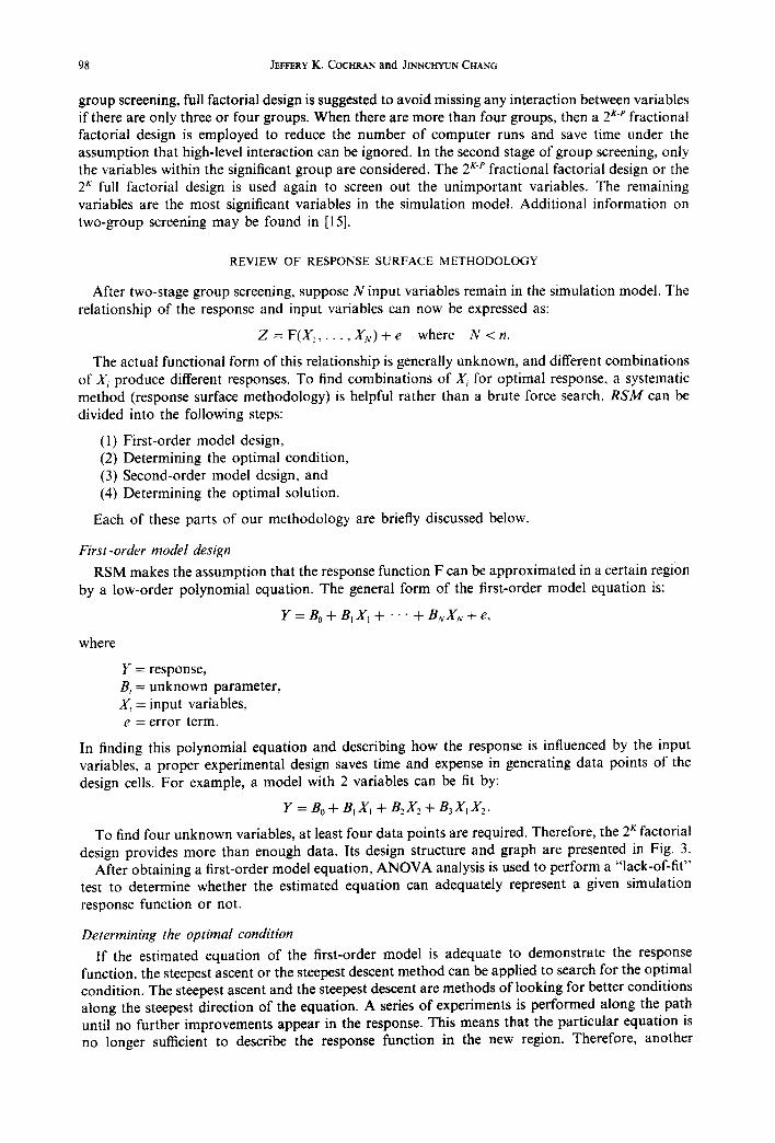
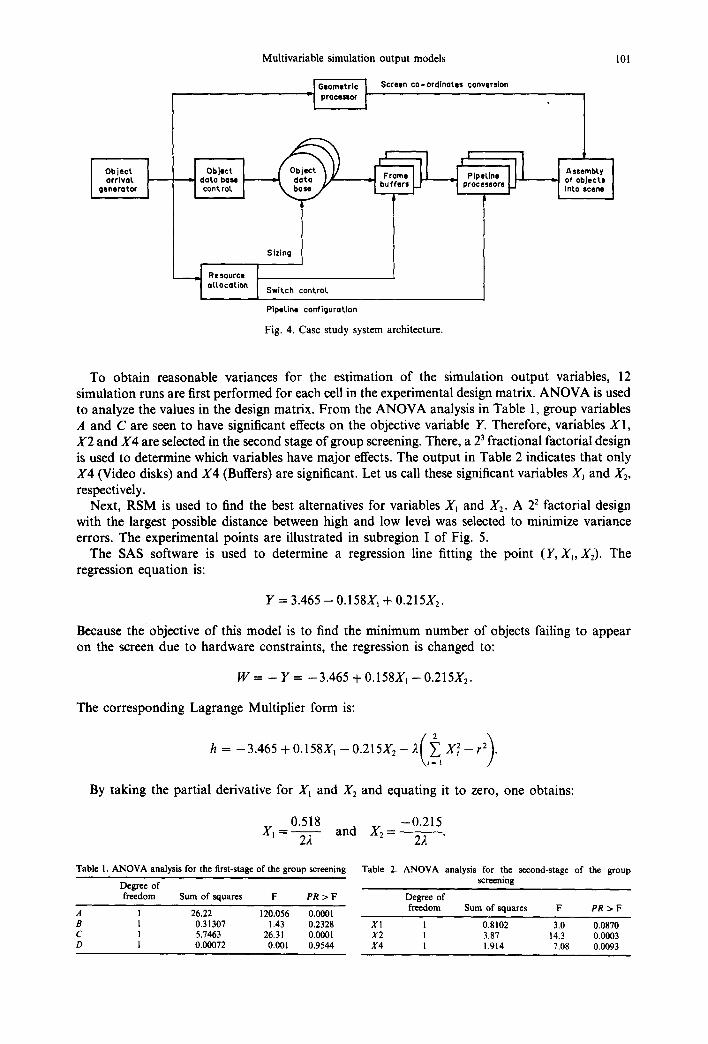
a m i n i m u m cost. F igure 4 summar izes the in te r re la t ionsh ips a m o n g those devices to be s imulated. W e now proceed to show how the g roup screening and R S M methods are used to find the op t imal c omb ina t i ons o f those devices with m i n i m u m cost and m a x i m u m per formance .

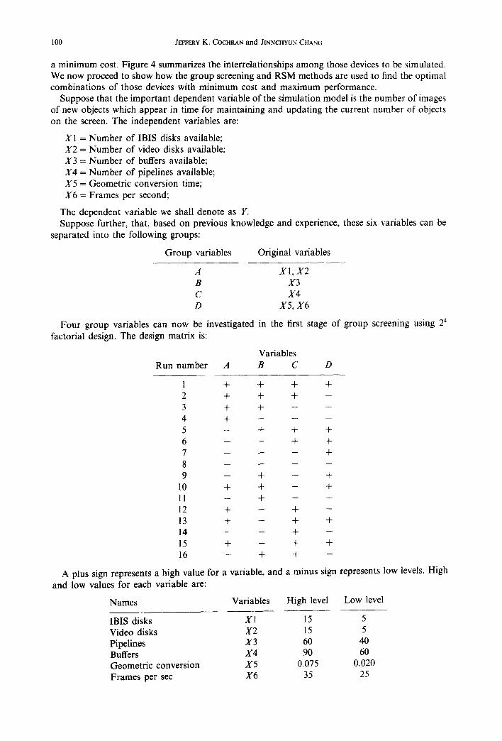
Suppose that the i m p o r t a n t dependen t var iable o f the s imula t ion mode l is the number o f images o f new objects which a p p e a r in t ime for ma in t a in ing and upda t ing the current number o f objects on the screen. The independen t var iables are:

X1 = N u m b e r o f IBIS disks avai lable; X2 = N u m b e r o f video disks avai lable; X3 = N u m b e r o f buffers avai lable; X4 = N u m b e r o f pipel ines avai lable; X5 = Geomet r i c convers ion time; X6 = F r a m e s per second;

The dependen t var iab le we shall denote as Y. Suppose further , that , based on prev ious knowledge and experience, these six var iables can be

sepa ra t ed into the fol lowing groups:

G r o u p var iables Original var iables

A X1, X2 B X3 C X 4 D X5, X6

F o u r g roup var iables can now be invest igated in the first s tage o f g roup screening using 2 4

fac tor ia l design. The design mat r ix is:

Var iables

Run n u m b e r A B C D

1 + + + +

2 + + + - 3 + + - - 4 + - - -

5 - + + + 6 - - + + 7 - - - +

. . . .

9 - + - + 10 + + - + 11 - - + - - - -

1 2 + - + - 13 + - + + 14 - - + -

1 5 + - + + 16 - + + -

A plus sign represents a high value for a var iable , and a minus sign represents low levels. High

and low values for each var iable are:

N a m e s Var iables High level Low level

IBIS disks X1 15 5 Video disks X2 15 5 Pipelines X3 60 40 Buffers X 4 90 60 Geome t r i c convers ion X5 0.075 0.020 F r a m e s per sec X6 35 25

Multivariable simulation output models

- i Geometric I Screen co-ordinates conversion I proco~or I

101

Object I arrival generator

i I

_ Pipl proc~

a, oc-- [ q Switch control

PipeLine configuration

Fig . 4. Case study system architecture.

Assl nbty 1 Line of ol eels | ssore into cone I

To obtain reasonable variances for the estimation of the simulation output variables, 12 simulation runs are first performed for each cell in the experimental design matrix. ANOVA is used to analyze the values in the design matrix. From the ANOVA analysis in Table 1, group variables A and C are seen to have significant effects on the objective variable Y. Therefore, variables X1, ,V2 and X4 are selected in the second stage of group screening. There, a 2 ~ fractional factorial design is used to determine which variables have major effects. The output in Table 2 indicates that only X4 (Video disks) and X4 (Buffers) are significant. Let us call these significant variables Xj and -t"2, respectively.

Next, RSM is used to find the best alternatives for variables X~ and X2. A 22 factorial design with the largest possible distance between high and low level was selected to minimize variance errors. The experimental points are illustrated in subregion I of Fig. 5.

The SAS software is used to determine a regression line fitting the point (Y, Xl, X2). The regression equation is:

Y = 3.465 - 0.158X1 + 0.2157(2.

Because the objective of this model is to find the minimum number of objects failing to appear on the screen due to hardware constraints, the regression is changed to:

W = - Y = - 3 . 4 6 5 + 0.158X1 - 0.215X2.

The corresponding Lagrange Multiplier form is:

h=-3"465+O'158X~-O'215X2-2(~lX~-r2)'i By taking the partial derivative for Xt and X2 and equating it to zero, one obtains:

0.518 - -0 .215 X I = - - and X 2 = - -

22 22

Table 1. ANOVA analysis for the first-stage of the group screening

Degree of freedom Sum of squares F PR > F

A 1 26.22 120.056 0.0001 B 1 0.31307 1.43 0.2328 C 1 5.7463 26.31 0.0001 D l 0.00072 0.001 0.9544

Table 2. ANOVA analysis for the second-stage of the group screening

Degree of freedom Sum of squares F PR > F

XI 1 0.8102 3.0 0.0870 X2 l 3.87 14.3 0.0003 X4 l 1.914 7.08 0.0093

102 JEFFERY K . COCHRAN a n d JINNCHYUN CHANG

i I

/ /

/ /

/ /

f t \ \ t

/ /

/

/ \

/ / \~ I I I I ~ , . / 5 I 5.5 / 6

I I s ~ > / a / i / t 1 9 3 I / / \ - Subre~lo.,~ / / /

/ / / / / /

/ / / Video disks

Fig. 5. S e a r c h p rocesses for the o p t i m a l so lu t ion .

X \

I I I I I I

/ r /

Variable X2 is selected to determine the value 2 because the coefficient of X2 is greater than X~. When the real value of X2 increases one unit, the coded value of X2 increases 0.1 unit. Therefore,

and

-0.215 ), - = --0.01072

2x2

0.158 X1 . . . . 0.0736.

22

The searching path of steepest descent is shown in Table 3. The smallest value of response variable Y is 4.0091. Taking whole numbers for Xl and )(2, the

corresponding optimal values are:

XI = 7;

)(2 = 59.

Then, the search is moved from subregion I to subregion II. The results of subregion II show that the data no longer fit the regression line. Therefore, a CCD is used to find the second order polynomial equation. The SAS output indicates that the equation is:

Y = 4.067 + 0.273X~ - 0.1361X2 - 0.1555X~ + 0.131X~

Table 3. Path of steepest descent for variables X~ and X 2

XI X2 Y

base 10 50 5.8039 A --0.368 1 base + IA 9.632 51 5.2823 base + 2A 8.896 52 5.1781 base + 3A 8.578 53 4.3937 base + 4A 8.578 54 4.2240 base + 5A 8.156 55 4.1960 base + 6A 7.792 56 4.1634 base + 7A 7.424 57 4.1360 base + 8A 7.056 58 4.1100 base + 9A 6.688 59 4.0091 b a s e + 10A 6.320 60 4.1533

Multivariable simulation output models 103

To find the minimiz ing po in t o f this equat ion , par t ia l der ivat ives with respect to X~ and X 2 were again taken and set equal to zero, and the resul t ing equat ions were solved. The solut ion is:

Xi = 7.0259;

Y = 4.052;

X2 = 59.2181.

These results indicate tha t seven video disks and sixty buffers are op t imal . In this example , we have taken the closest whole number and set the rest o f the devices at their low level to minimize

cost.

CONCLUSION

Simula t ion is of ten to es t imate the pe r fo rmance in different s i tuat ions o f a real wor ld model . One d r a w b a c k o f the s imula t ion a p p r o a c h is tha t it can only s imulate condi t ions using predefined variables . Significant factors p roduc ing the ou tpu t o f a mode l can be ob ta ined by tr ial and e r r o r - - w h i c h means compu te r runs and cost. Response surface m e t h o d o l o g y provides a s t rong and efficient technique for ana lyz ing s imula t ion outputs , but the calcula t ing processes become very compl i ca t ed and t ime-consuming when a s imula t ion mode l has many variables. Two-s tage g roup screening g roup screening m e t h o d o l o g y was deve loped before compu te r s imula t ion exper iments . G S uses exper iment design to e l iminate u n i m p o r t a n t var iables by g roup ing s imilar var iables together . The flight s imula to r example in this pape r shows tha t our exper imenta l design a p p r o a c h to the g roup screening me thod can great ly reduce s imula t ion effect. The mode l has six input variables . I f a 2 k - l exper imenta l design is used, 384 compu te r runs are needed to detect significant variables . The g roup screening me thod used only 288 runs. In general , each run m a y be very t ime consuming. In our small case s tudy, 3 C P U sec on an IBM 4381 supe r -min icompute r and 5 c lock-minutes o f setup t ime were required per run. Such saving can poten t ia l ly be substant ia l . The more input var iables tha t are in the mode l and the more advance knowledge abou t re la ted varaibles for grouping , the more compu te r runs can be saved.

Acknowledgements--We wish to thank the referees for their comments which improved this paper. We also wish to thank David Sykes at the Honeywell Training and Control Services Center for the opportunity to work on his Visual System Component Development Program in Grant No. 840959.

REFERENCES

1. A. M. Law and W. D. Kelton. Simulation Modeling and Analysis, McGraw-Hill, New York (1982). 2. J. P. C. Kleijnen. Statistical Tools for Simulation Practitioners, Marcel Dekker, New York (1987). 3. R. H. Myers. Response Surface Methodology, Allyn & Bacon, Boston (1971). 4. W. L. Biles. Design of simulation experiments. Winter Simulation Conf. 99-104 (1984). 5. A. I. Khuri and J. A. Cornell. Response Surfaces, Marcel Dekker, New York (1987). 6. D. E. Smith. An empirical investigation of optimum-seeking in the computer simulation situation. Opns Res. 21,

475-497 (1973). 7. D. E. Smith. Automatic optimum-seeking program for digital simulation. Simulation 27, 27-31 (1976). 8. M. H. Safizadeh and B. M. Thornton. Optimization in simulation experiments using response surface methodology.

Computers Ind. Engng 11-27 (1984). 9. D. E. Smith and C. A. Mauro. Factor screening in computer simulation. Simulation 4, 54~2 (1982).

10. G. S. Watson. A study of the group screening method. Technometrics 372-388 (1961). 11. J. P. C. Kleijnen. Simulation with too many factors: review of random and group screening designs. Fur. J. Opns Res.

31, 31-36 (1987). 12. C. A. Mauro and D. E. Smith. The performance of two-stage group screening in factor screening experiments.

Technometrics 24(4), 325-330 (1982). 13. L. Lin and J. K. Cochran. Optimization of a complex flow line for print circuit board fabrication by computer

simulation. J. Manuf. Syst. 6(I), 47-57 (1987). 14. D. C. Montgomery and W. Ginner. Factor screening methods in computer simulation experiments. Winter Simulation

Conf. 347-358 (1979). 15. C. A. Mauro. On the performance of two-stage group screening experiments. Technometrics 26(3), 255-264 (1984). 16. G. E. P. Box and N. R. Draper. Empirical Model-Building and Response Surfaces, Wiley, New York (1987). 17. J. K. Cochran, N. F. Hubele and D. J. Sykes. A new generation of flight simulators: design configuration with

discrete-event simulation. SCS Simulation Series 18(4), 234-238 (1987). 18. N. F. Hubele and J. K. Cochran. A discrete event simulation model for the visual system component development

program. Final Report for Honeywell, Inc., Arizona State University (1986).