11

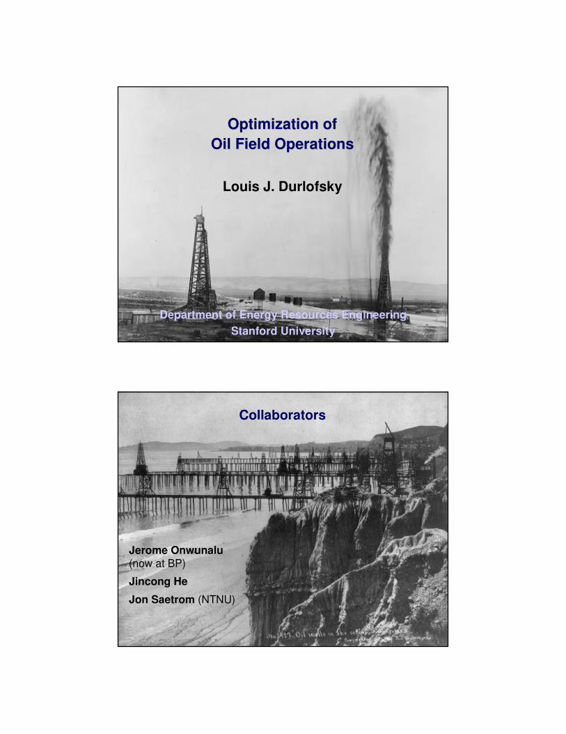
Optimization of Optimization of

Oil Field OperationsOil Field Operations

Louis J. Durlofsky

Department of Energy Resources Engineering

Stanford University

2

Collaborators

Jerome Onwunalu

(now at BP)

Jincong He

Jon Saetrom (NTNU)

3

Smart Field Modeling

Reservoir Data

Update Model

Optimize Well Settings

Set Well Controls

Field Development Optimization

• Optimization highly intensive computationally

44

Outline

• Field development (well placement) optimization

– Particle swarm optimization (PSO) algorithm

– Well pattern optimization

• Production optimization

– Trajectory piecewise linearization (TPWL) for surrogate modeling

– Generalized pattern search method with TPWL

• Conclusions

5

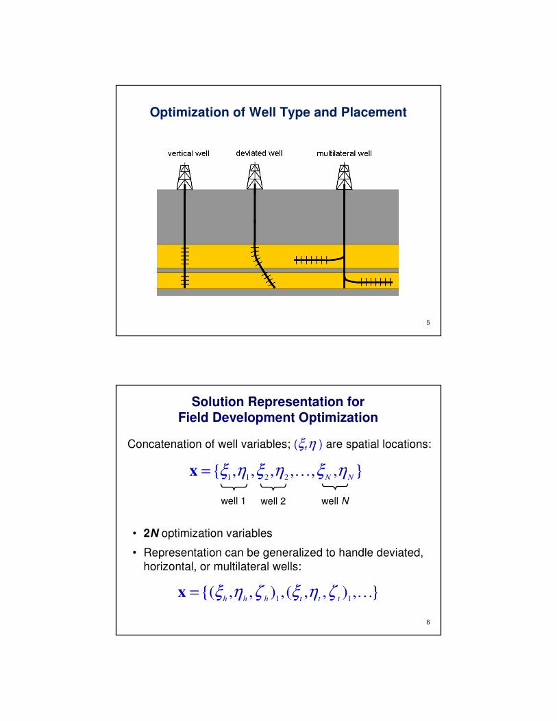
Optimization of Well Type and Placement

6

Solution Representation for Field Development Optimization

• 2N optimization variables

• Representation can be generalized to handle deviated, horizontal, or multilateral wells:

Concatenation of well variables; (ξ,η ) are spatial locations:

},,,,,,{2211 NN

ηξηξηξ K=x

well 1 well 2 well N

},),,(,),,{(11K

ttthhhζηξζηξ=x

7

Particle Swarm Optimization (PSO)

• Developed originally by Kennedy & Eberhardt (1995)

• Models social behavior in animals and entails a cooperative search strategy (population-based like Genetic Algorithm)

• Successfully applied for subsurface flow optimization (groundwater remediation) by Mattot et al. (2006)

http://inlinethumb61.webshots.com

8

PSO Solution Iteration

xi – solution, vi – particle velocity, k – iteration, ∆t = 1

• Particle velocity has 3 contributions:

9

Particle Swarm Optimization (2D Search Space)

10

PSO ‘Neighborhood’ Topologies

11

Genetic Algorithm (GA) Operations

}Population and selection:

Crossover:

Mutation:

12

PSO versus GA for Well Placement

• In our tests, PSO generally outperformed GA

• 2 dual-lateral producers

– Average PSO NPV (from 5 runs) 19% higher than GA

• 4 deviated producers

– Average PSO NPV (from 5 runs) 7% higher than GA

13

Optimization Example: PSO versus GA

• Find well location and type (20 wells) to maximize net present value (NPV)

• 2D model, 100 x 100 blocks, oil-water simulation

• Swarm (population): 50; iterations (generations): 100

• Perform 4 runs for each algorithm

• 60 optimization variables

},,,,,,,,,{222111 NNN

iii ηξηξηξ K=x

14

Optimization Results: PSO and GA

- · - PSO –– GA

15

Well Locations and Types: PSO and GA

16

Solution Representation for Multiple Wells

• Number of optimization variables increases with well count – high computational expense

• Well count N must be specified (this should also be an optimization variable)

• May be difficult to enforce distance constraints

Concatenation of well variables:

},,,,,,{2211 NN

ηξηξηξ K=x

well 1 well 2 well N

17

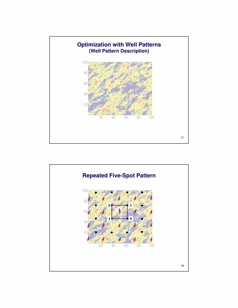
Optimization with Well Patterns(Well Pattern Description)

18

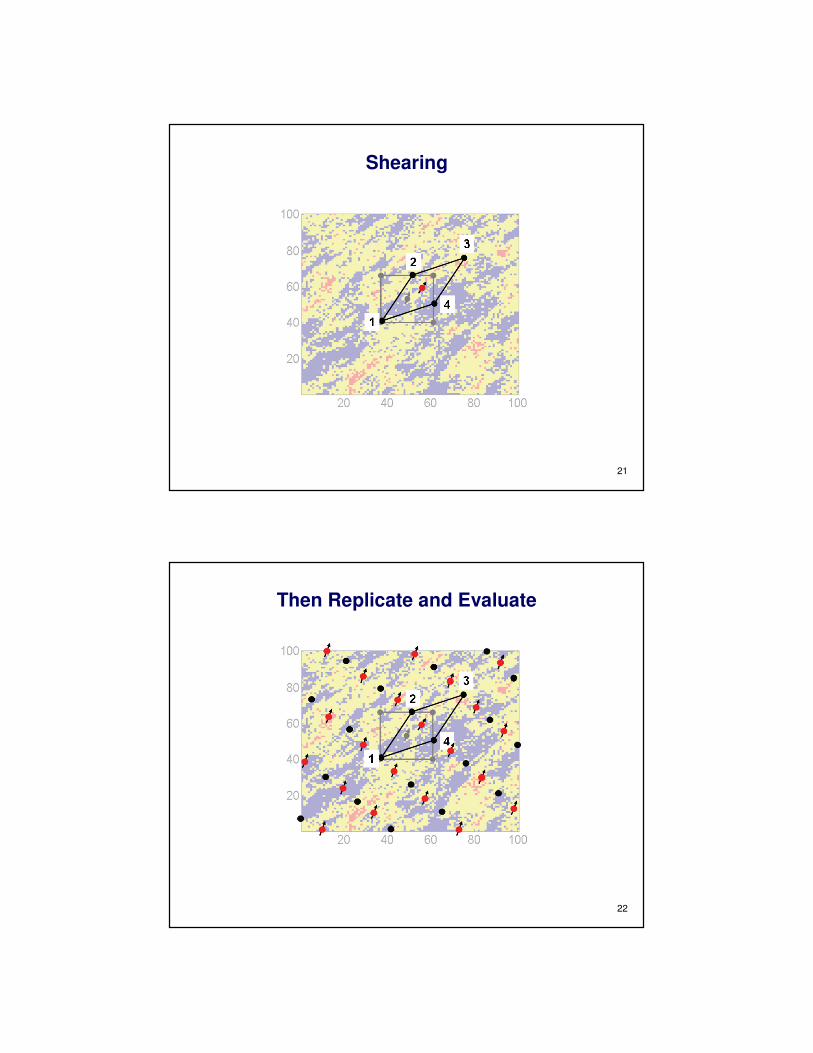
Repeated Five-Spot Pattern

19

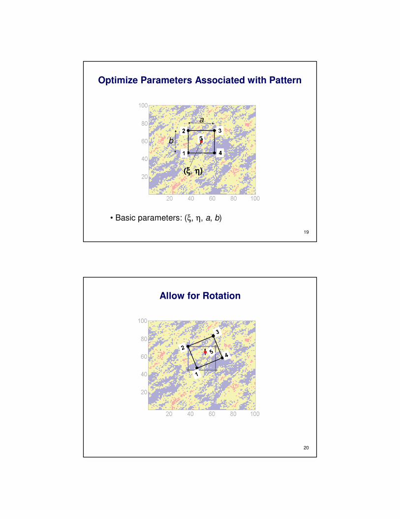
Optimize Parameters Associated with Pattern

• Basic parameters: (ξ, η, a, b)

(ξ(ξ(ξ(ξ, ηηηη)

a

b

20

Allow for Rotation

21

Shearing

22

Then Replicate and Evaluate

23

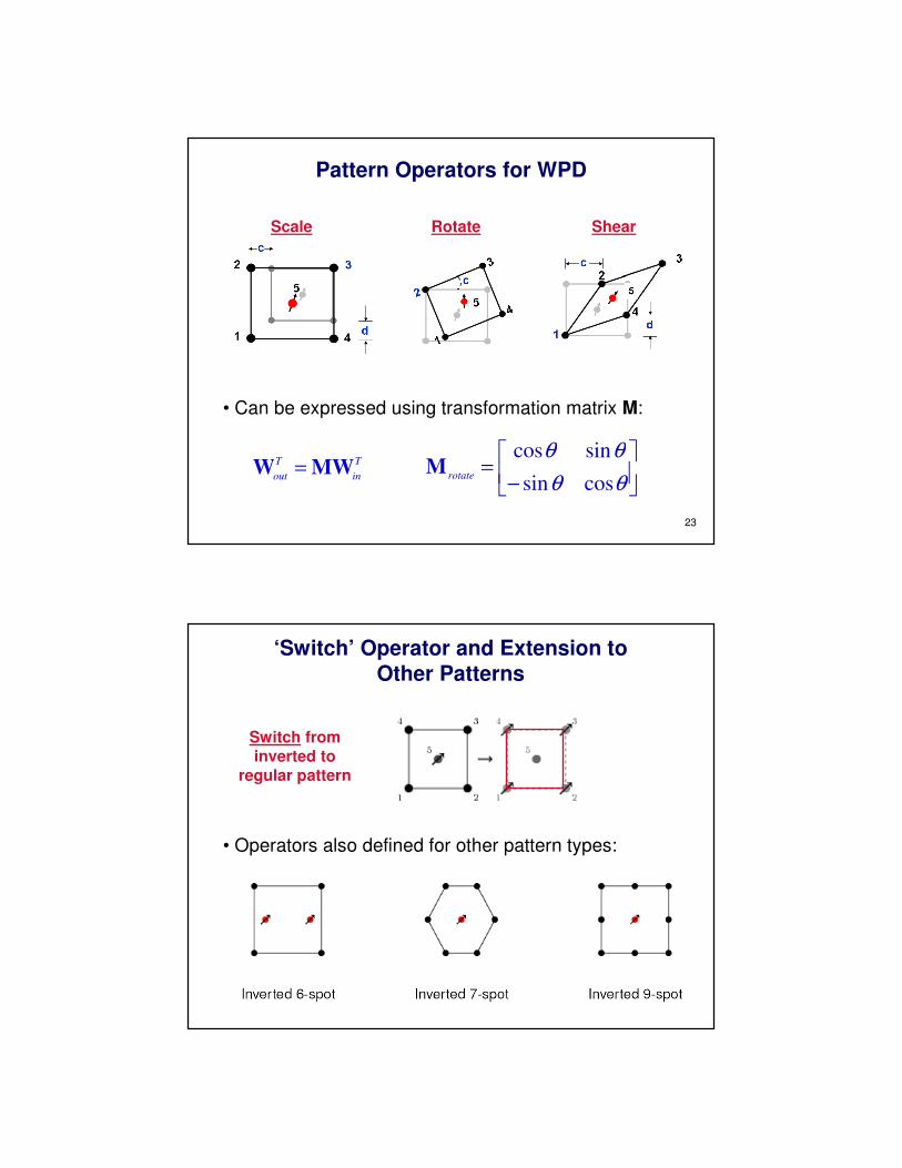
Pattern Operators for WPD

T

in

T

outMWW =

−=

θθ

θθ

cossin

sincosrotate

M

Scale Rotate Shear

• Can be expressed using transformation matrix M:

24

‘Switch’ Operator and Extension to Other Patterns

Switch from inverted to

regular pattern

• Operators also defined for other pattern types:

25

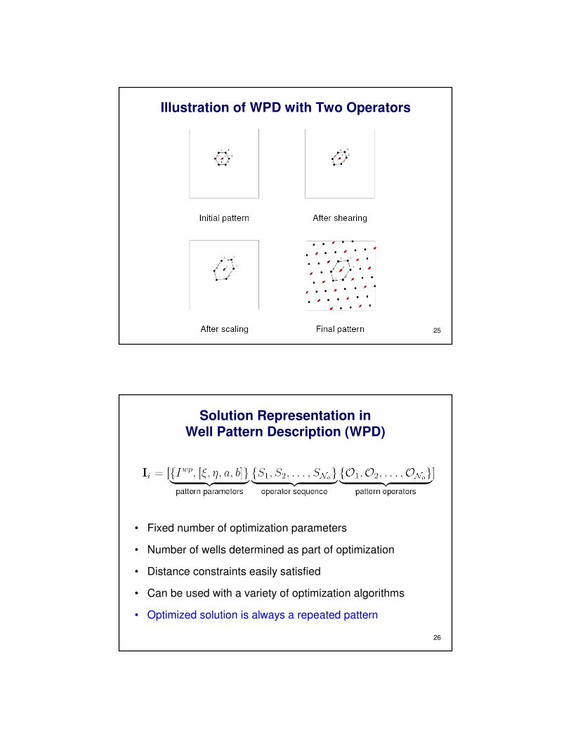
Illustration of WPD with Two Operators

26

Solution Representation in Well Pattern Description (WPD)

• Fixed number of optimization parameters

• Number of wells determined as part of optimization

• Distance constraints easily satisfied

• Can be used with a variety of optimization algorithms

• Optimized solution is always a repeated pattern

27

Well-by-Well Perturbation (WWP)

• Same number of variables as concatenation approach but much smaller search space, and N is specified

28

Example 1: Problem Set Up

• 2D model, 100 x 100 grid blocks

• Oil-water system, 10 years of production

• Injector BHP: 6000 psi, Producer BHP: 1000 psi

• Maximize NPV; run optimization multiple times

permeability field

29

Algorithm Performance – Pattern Optimization(one pattern operator)

• Best NPV using standard well patterns: $2151 MM

30

Example 1: Optimization Results

injector

31

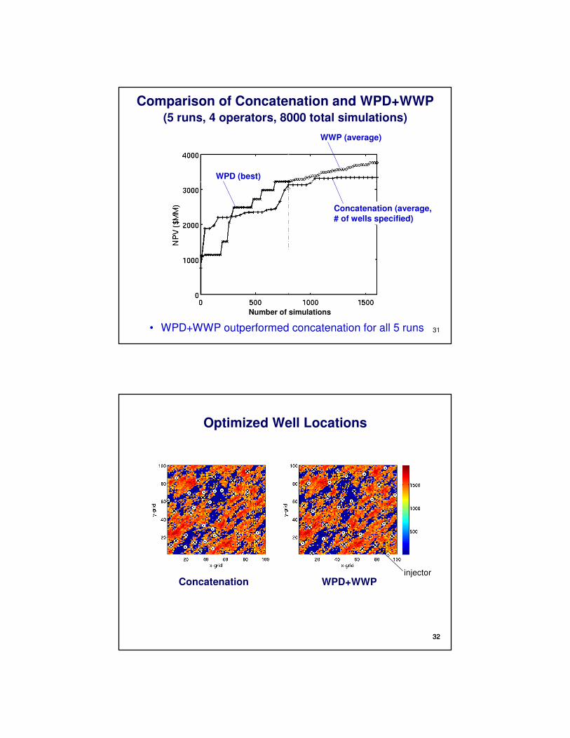
Comparison of Concatenation and WPD+WWP(5 runs, 4 operators, 8000 total simulations)

• WPD+WWP outperformed concatenation for all 5 runs

Concatenation (average,

# of wells specified)

WWP (average)

WPD (best)

Number of simulations

32

Optimized Well Locations

32

Concatenation WPD+WWPinjector

33

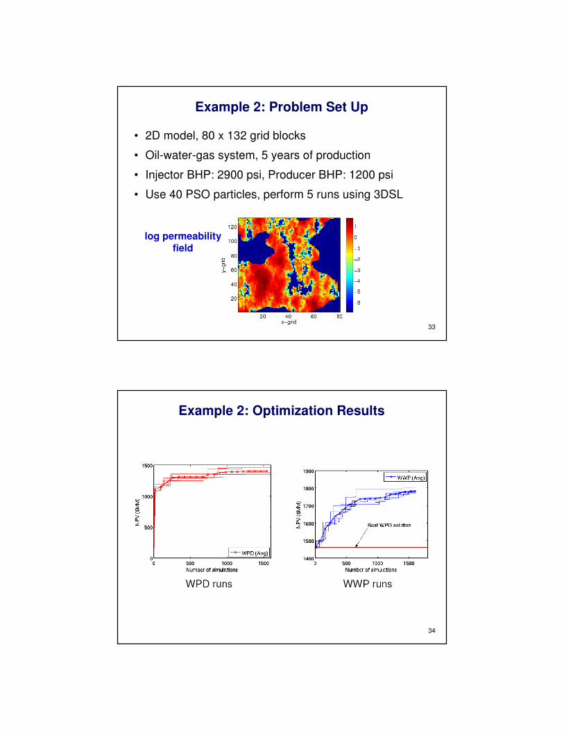
Example 2: Problem Set Up

• 2D model, 80 x 132 grid blocks

• Oil-water-gas system, 5 years of production

• Injector BHP: 2900 psi, Producer BHP: 1200 psi

• Use 40 PSO particles, perform 5 runs using 3DSL

log permeability

field

34

Example 2: Optimization Results

35

Example 2: Optimization Results

WPD (pattern)

WWP after WPD

WPD+WWP performance

36

Example 2: Well Locations

injector

3737

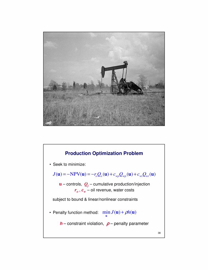
Production Optimization Problem

• Seek to minimize:

u – controls, Qj – cumulative production/injection

ro , cw – oil revenue, water costs

)()()()(NPV)( uuuuu wiwiwpwpoo QcQcQrJ ++−=−=

subject to bound & linear/nonlinear constraints

38

• Penalty function method: )()(min uuu

hJ ρ+

h – constraint violation, ρρρρ – penalty parameter

39

Oil-Water Flow Equations

( ) 0

=+∇⋅∇−∂

∂jj

jqp

t

Skλφ

• Mass balance equations for j = oil, water

Sj - phase saturation (volume fraction), p - pressure

λλλλj (Sj ) - phase mobility, k - permeability tensor, qj - source

• Discretize: x - states (p, Sw), u - controls (pwell),

O(105-106) grid blocks

( ) ( ) ( ) ( ) 0,,,,111111 =++= ++++++ nnnnnnnn uxQxFxxAuxxg

, gδJ −= xgJ ∂∂=• Newton’s method:

4040

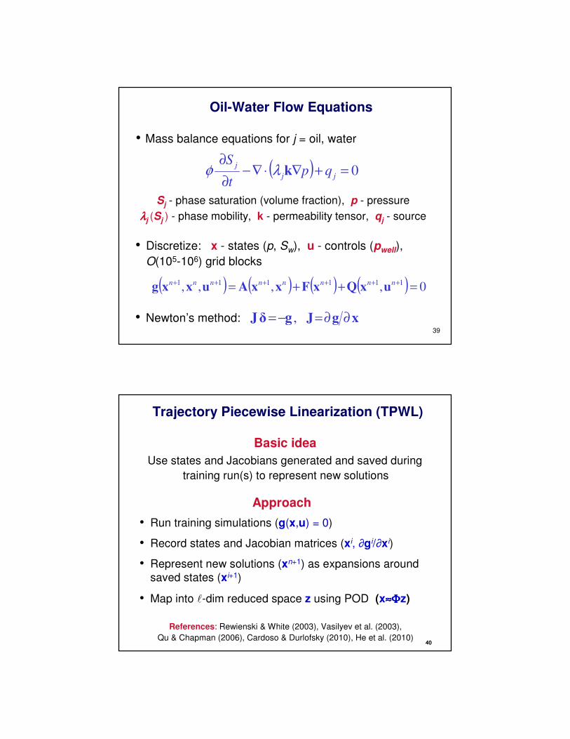
Use states and Jacobians generated and saved during

training run(s) to represent new solutions

Trajectory Piecewise Linearization (TPWL)

• Run training simulations (g(x,u) = 0)

• Record states and Jacobian matrices (xi, ∂gi/∂xi)

• Represent new solutions (xn+1) as expansions around saved states (xi+1)

• Map into l-dim reduced space z using POD (x≈≈≈≈ΦΦΦΦz)

Approach

Basic idea

References: Rewienski & White (2003), Vasilyev et al. (2003),

Qu & Chapman (2006), Cardoso & Durlofsky (2010), He et al. (2010)

4141

Linearization around Saved States

x1

x2

2D state spacei = 1 i = 2

i = 3i = 4

i = 5

i = 6

i =7

i = 8

u0

• Save xi and ∂gi/∂xi (u0)

u1

• Represent solutions for u1 using xi and ∂gi/∂xi

4242

TPWL for Reservoir Flow Equations

01111 =++= ++++ nnnn

QFAg

Discretized flow equations:

Linearized representation for new state xn+1:

( ) ( ) ( )11

1

11

11

1

1

11 ++

+

++++

+

+++ −

∂

∂+−

∂

∂+−

∂

∂+≅ in

i

iin

i

iin

i

iin uu

u

gxx

x

gxx

x

ggg

x: states (p, Sw) u: controls (BHPs)

4343

Expansion around Saved States

• Linearized representation:

( ) ( ) ( )

−

∂

∂+−

∂

∂−=− ++

+

+++++ 11

1

11111 in

i

iin

i

iini uu

u

Qxx

x

AxxJ

• POD (SVD) applied to snapshot matrix: x ≈≈≈≈ ΦΦΦΦz

• TPWL representation (reduced space, multiply by ΦΦΦΦT ):

( ) ( ) ( )

−

∂

∂+−

∂

∂−= ++

+

++−+++ 11

1

111111 in

r

i

iin

r

i

ii

r

inuu

u

Qzz

x

AJzz

ΦJΦJ 11 ++ = iTi

r(llll ×××× llll) llll ~ O(102 –103)

44

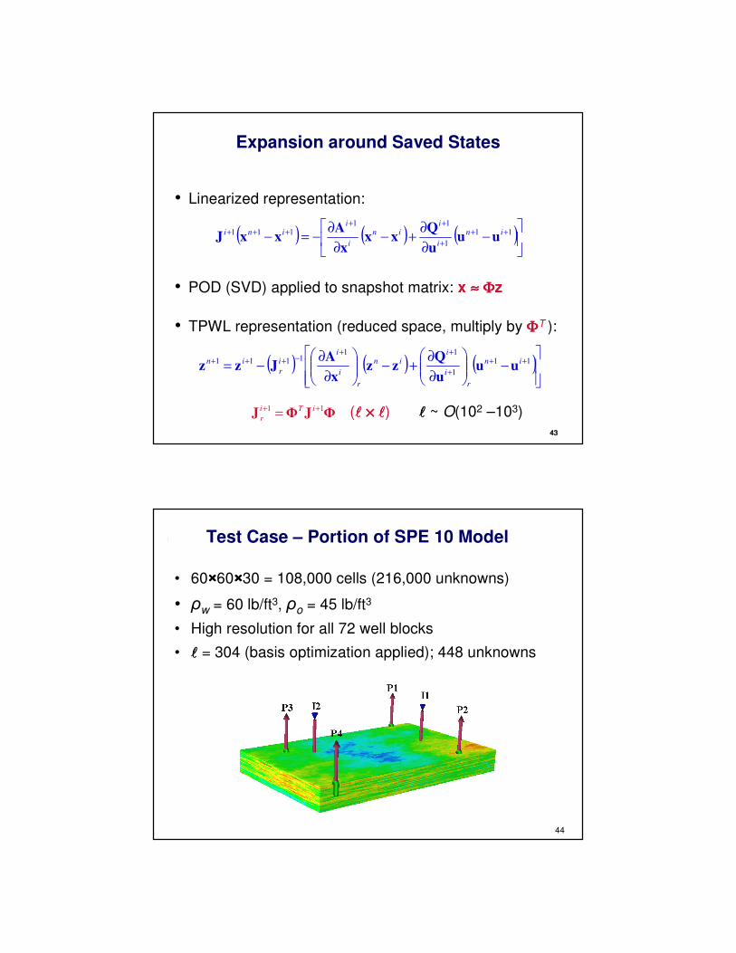
Test Case – Portion of SPE 10 Model

• 60××××60××××30 = 108,000 cells (216,000 unknowns)

• ρw = 60 lb/ft3, ρo = 45 lb/ft3

• High resolution for all 72 well blocks

• llll = 304 (basis optimization applied); 448 unknowns

45

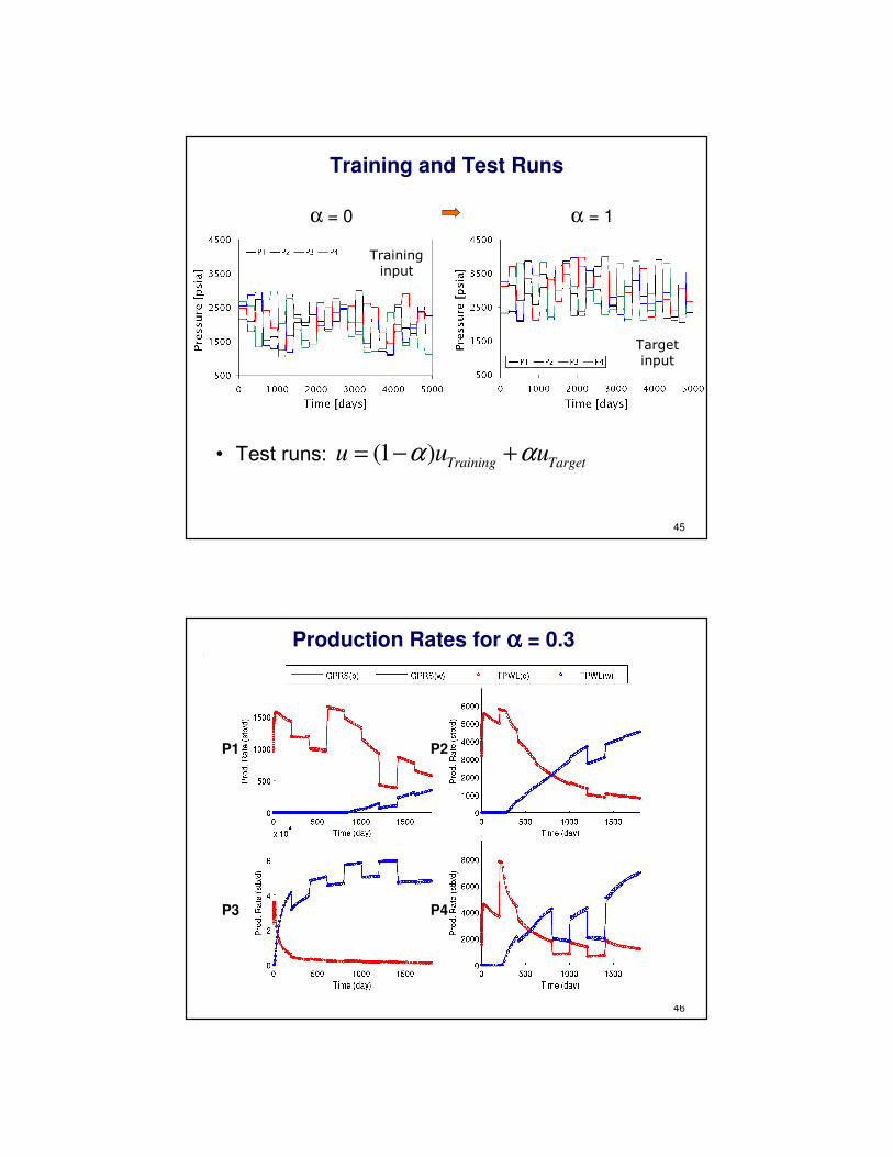
Training and Test Runs

Training input

Target input

α = 1α = 0

• Test runs: (1 )Training Target

u u uα α= − +

46

Production Rates for αααα = 0.3

P1 P2

P3 P4

47

Production Rates for αααα = 0.5

GPRS/CPR TPWL

Run Time ~1 hr ~2 sec

P1 P2

P3 P4

48

TPWL as a Proxy for Optimization

(Kolda et al., 2003)

• Apply TPWL for direct search methods

• Perform an initial training simulation

• Retrain TPWL after specified number of iterations, “distance” from last training, etc.

Generalized Pattern Search

(GPS)

TrainingRetrain

49

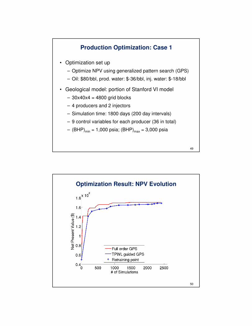
Production Optimization: Case 1

• Optimization set up

– Optimize NPV using generalized pattern search (GPS)

– Oil: $80/bbl, prod. water: $-36/bbl, inj. water: $-18/bbl

• Geological model: portion of Stanford VI model

– 30x40x4 = 4800 grid blocks

– 4 producers and 2 injectors

– Simulation time: 1800 days (200 day intervals)

– 9 control variables for each producer (36 in total)

– (BHP)min = 1,000 psia; (BHP)max = 3,000 psia

50

Optimization Result: NPV Evolution

51

MethodNPV (initial)

$106

NPV (final)

$106

# of full

simulations

Full-order GPS 49.9 170.1 2500

TPWL-guided GPS 49.9 169.0 15

TPWL model construction ~ 2×time for training run

Optimization Result: NPV Summary

52

Optimization Results: Final BHP Schedules

53

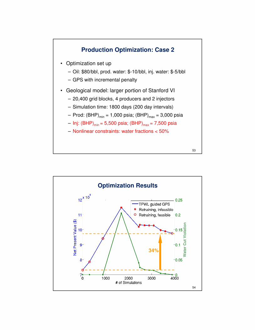
Production Optimization: Case 2

• Optimization set up

– Oil: $80/bbl, prod. water: $-10/bbl, inj. water: $-5/bbl

– GPS with incremental penalty

• Geological model: larger portion of Stanford VI

– 20,400 grid blocks, 4 producers and 2 injectors

– Simulation time: 1800 days (200 day intervals)

– Prod: (BHP)min = 1,000 psia; (BHP)max = 3,000 psia

– Inj: (BHP)min = 5,500 psia; (BHP)max = 7,500 psia

– Nonlinear constraints: water fractions < 50%

54

Optimization ResultsW

ate

r C

ut

Vio

lati

on

34%

55

Optimization Results: Injector BHP Schedules

MethodNPV (initial)

$106

NPV (final)

$106

# of full

simulations

TPWL-guided GPS

729 975 ~12

5656

Summary and Future Work

• Applied particle swarm optimization (PSO) for determining placement of new wells

• Devised new treatments for optimizing multiwell (field) development problems

• Demonstrated use of TPWL (trajectory piecewise linearization) procedure for fast reservoir simulation

• Incorporated TPWL into generalized pattern search optimization of oil production

• Future work: meta-optimization techniques for use with PSO; enhance TPWL and clarify criteria for retraining; combine field development & production optimization