optimization of wireless power transfer systems enhanced ... · index terms convex optimization,...

IEEE TRANSACTIONS ON ANTENNAS AND PROPAGATION 1

Optimization of Wireless Power Transfer SystemsEnhanced by Passive Elements and Metasurfaces

Hans-Dieter Lang, Student Member, IEEE, and Costas D. Sarris, Senior Member, IEEE

Abstract—This paper presents a rigorous optimization tech-nique for wireless power transfer (WPT) systems enhanced bypassive elements, ranging from simple reflectors and intermedi-ate relays all the way to general electromagnetic guiding andfocusing structures, such as metasurfaces and metamaterials. Atits core is a convex semidefinite relaxation formulation of theotherwise nonconvex optimization problem, of which tightnessand optimality can be confirmed by a simple test of its solutions.The resulting method is rigorous, versatile, and general — it doesnot rely on any assumptions. As shown in various examples, itis able to efficiently and reliably optimize such WPT systems inorder to find their physical limitations on performance, optimaloperating parameters and inspect their working principles, evenfor a large number of active transmitters and passive elements.

Index Terms—Convex Optimization, Multiple Transmitters,Passive Couplers, Power Transfer Efficiency, Semidefinite Pro-gramming, Tight Relaxation, Wireless Power Transfer.

I. INTRODUCTION

W IRELESS power transfer (WPT) systems have beeninvestigated in various forms, contexts and for various

applications [1]–[4]. A large variety of unique solutions forpowering and charging devices in an untethered fashion hasbeen proposed; ranging from applications such as chargingmobile devices [5] to electric vehicles [6]–[8] and includingcharging, operating as well as communicating with biomedicalimplants [9].

However, among other constraints, the performance — mostcommonly measured by the power transfer efficiency (PTE),the efficiency at which the power can be transferred from thetransmitter(s) to the receiver — considerably limits the rangeof such applications. Usually, PTEs high enough for practicalapplications are confined to distances between transmitter(s)and receiver(s) in the order of fractions of the wavelength atthe operating frequency as well as to dimensions comparableto those of the transmitter and receiver coils [5].

Various attempts to mitigate this problem and increase thePTE or extend the range of high PTE have been proposed.A popular method to enhance PTE involves introducing pas-sive elements in the proximity of the transmitter(s) and thereceiver [10], acting as relay elements or as parasitic elementsthat can enlarge the effective aperture of the transmitter.

Manuscript received May xx, 2016; revised Month xx, 2016; acceptedMonth xx, 2016. Date of publication: Month zz, 2016. Current version: Later00

The authors are with the Electromagnetics Group of the Department ofElectrical and Computer Engineering, University of Toronto, ON, M5S 3G4,Canada, (e-mail: [email protected], [email protected]).

Color versions of one or more of the figures in this paper are availableonline at http://ieeexplore.ieee.org.

Digital Object Identifier XX.YYYY/TAP.2016.ZZZZZZZ

Multiple passive elements can be used cooperatively; forexample to form near-field guiding structures [11]–[15] orprovide more general functions associated with metasurfacesor metamaterials [16]–[18].

As will be shown, the optimization of such systems isnot a trivial task; the standard formulations of the requiredpassivity and power constraints are nonconvex. This rendersthe whole problem unsolvable in general, particularly fora large number of unknowns (e.g. the number of passiveelements). Here, however, a convex relaxation formulation isderived, which essentially constitutes a general and rigorouswork-around to this problem. Furthermore, a simple test of thesolution confirms tightness (meaning exact representation ofthe original problem) and hence, that the true global optimumhas been found.

The resulting powerful and rigorous optimization methodgeneralizes the previously presented optimization techniquefor WPT systems with multiple active transmitters [19]. Hence,it can be used to investigate the maximum performance of aparticular system with multiple active transmitters and passiveelements and to obtain the corresponding optimal operatingparameters (i.e. currents and loading reactances). Furthermore,using an outer loop optimization, the optimum load resistancecan also be found, leading to the maximum achievable PTEof the system; the absolute limit on the performance.

The outline of this paper is as follows: After a shortintroduction, the optimization problem of passively-enhancedWPT systems is presented. The convex semidefinite relaxationis then derived and a simple test for tightness is given. In theresults section, three numerical examples prove the validityand versatility of the method: First, the case where additionalpassively excited transmitters are added behind the activetransmitter is considered. Second, optimal relay configurationsare treated, useful for both high-efficiency range extension aswell as for misalignment mitigation. Lastly, the enhancementby general passive metasurfaces is discussed; proving themethod’s capability to handle a large number of passiveelements. At the end, final remarks and conclusions are given.

Remarks on the notation: Thin italic letters represent scalarvariables, bold small letters refer to vectors, bold capital lettersare matrices; vT stands for the transpose of the vector v, whilevH stands for its Hermitian (conjugate transpose). The symbol () is used to denominate positive (semi-) definitenessof matrices, respectively. A star (·)? marks the optimizedarguments leading to the optimal solution, while a bar (a)is used to denote the complex conjugate. Lastly, ’program’ isused as a synonym for ’optimization problem’, as is commonin the context of mathematical optimization [20].

arX

iv:1

701.

0769

4v2

[m

ath.

OC

] 1

Mar

201

7


II. PRELIMINARIES

A. The MISO WPT System Model with Passive Elements

Fig. 1 depicts the general form of wireless power transfer(WPT) systems under consideration, incorporating multipleactive transmitters, multiple passive elements and a singlereceiver. Systems with multiple transmitters will be referredto as MISO (multiple-input, single-output) WPT systems, incontrast to SISO (single-input single-output) systems with onlya single transmitter.

C1

Loaded WPTS: Z = Z + jX + RL

Unloaded WPTS: Z

TX

Zt

i1

v1

i2

v2

i3v3 = 0

iN−1vN−1 = 0

C3 CN−1

CrC1

C2

irvr = 0

RL

RXzr

ztr

activ

eTX

pass

ive

RX

passive elements

Fig. 1. Loop-based MISO WPT system model with multiple active trans-mitters and passive elements: Core structure with unloaded impedance matrixZ, reactive components xn = −(ωCn)−1 (in case of capacitors), resistivereceiver load RL, and voltage sources vn. In this example, subscripts 1 and2 correspond to active transmitters (i.e. connected to a source), while 3 toN − 1 stand for the passive elements.

Let the (unloaded) impedance matrix Z ∈ CN×N of suchsystems be partitioned according to

Z =

Zt ztr

zTtr zr

=

Za Zap zar

ZTap Zp zpr

zTar zTpr zr

. (1)

The subscripts t and r refer to the transmitter and receiverparts, respectively, whereas the subscripts a and p refer to theactive and passive transmitters. Finally, the combinations tr,ap, ar and pr stand for the submatrices and vectors couplingtwo of these groups together.

Let all the nodes be numbered by n = 1, ... , N , whereN = A + P is the total number of nodes, including Aactive transmitters, n ∈ A (note that Za ∈ CA×A) and Ppassive nodes, n ∈ P— note that this includes both the passiveelements and the receiver.

The diagonals of Z, Zt, Za, and Zp as well as zr refer tothe loss resistances and self-reactances of the transmitters andreceiver, respectively. Typically, all Z ′′·,nn, z

′′r > 0 (inductive)

when considering systems of magnetically coupled loops orcoils; however, this is not a requirement. Likewise, all off-diagonal entries of Z are the coupling impedances due tothe mutual inductances jωMn,m. Generally each Mn,m is

complex (leading to non-zero real parts in the off-diagonalentries of Z), due to retardation effects, when the electricaldistance between the transmitter(s) and/or receiver are not verysmall.

For physical reasons, impedance matrices of passive recip-rocal circuits have to be positive-real [21]: The impedancematrix is symmetric Z = ZT and all Z′,Z′t,Z

′a,Z

′p 0 and

z′r > 0 (positive-definite), meaning positive quadratic forms,for example:

iHZ′i > 0 ∀ i ∈ CN (2)

Positive semidefiniteness ( 0) implies nonnegative (≥ 0)quadratic forms. For negative (semi-) definiteness the oppo-site signs and directions apply. In the context of impedancematrices, the mathematical property of positive-definitenessrepresents the fact that there is always some amount of lossin the system.

The process of adding reactances to each of the transmitterand receiver nodes as well as adding a resistive load as receiverwill be referred to as loading of the WPT system, where

Z = Z + jX + RL (3)

is the resulting loaded impedance matrix, marked by a hat. Infull detail, the voltages and currents v, i of the entire WPTsystem are related according to

vavp = 0vr = 0

︸︷︷︸v

=

Z+ j

Xa

Xp

xr

︸︷︷︸X

+

0

0RL

︸︷︷︸RL

iaipir

︸︷︷︸i

(4)

where the subscripts t, a, p, and r have the same meanings asexplained for (1). The real-valued diagonal matrix X containsthe load reactances, where positive and negative values referto inductive and capacitive loading, respectively. They aregrouped into the two diagonal matrices corresponding to theactive transmitters and passive elements as well as a scalar forthe receiver. The matrix RL is zero everywhere but at the lastdiagonal entry, corresponding to the receiver, where the loadresistance RL > 0 is located.

It is important to note that, since the load resistance RLis actually part of the impedance matrix, KVL states thatthe corresponding receiver voltage is zero, i.e. vr = 0 asexplicated in (4) and depicted in Fig. 1. The same is truefor the voltages of the passive couplers, vp = 0.

B. The Objective: Power Transfer Efficiency (PTE)

The central figure of merit when optimizing WPT systemsis the power transfer efficiency1 (PTE) [1]–[5], [7], [9]: theratio of the power PL transferred to the load RL, to the totaltransmit power provided by the source Pt

η =PLPt

=PL

Pl + PL=

RLRl +RL

. (5)

1It should be noted that the so defined PTE refers only to the electro-magnetic power transfer efficiency; i.e. the impacts of impedance matching,rectification and generation onto the total efficiency of an entire wireless powertransfer system are not considered, here.


Pl is the total power absorbed by the system, due to dissipationand radiation, modeled by the loss resistance Rl.

The goal of this paper is to find a mathematical methodto determine the absolute performance limits of such WPTsystems to wirelessly transfer power most efficiently viamultiple active transmitters and passive elements to a singlereceiver. Hence, the aim is to maximize the PTE, obtainedaccording to its definition (5) as the biquadratic form

η =12 iHRLi

12 (iHv)′

=iHRLi

iH(Z′ + RL)i. (6)

by finding the corresponding optimal voltages v and currentsi (real and imaginary parts) as well as loading elementsx = diag(X) =

[xa,xp, xr

]and RL. It is most convenient

to formulate the PTE in terms of the currents i. The voltagesv can be obtained from the currents using the fully loadedsystem (4). However, both are only meaningful solutions aslong as vr = 0 and vp = 0.

III. OPTIMIZATION

A. Port Impedance Matrices (PIMs)

The total power inserted into the system Pt in the denom-inator of (5) can be separated into the contributions of eachtransmitter as follows [19]:

Pt = Pl + PL =1

2(iHv)′ =

1

2iHZ′i

=∑

n

Pt,n =1

2

∑

n

iHTni (7)

where Tn are the (loaded) port impedance matrices (PIMs),and n denotes the port. Note that Tn = Tn, for all n exceptn = N (receiver), where TN = TN + RL; i.e. loading onlyaffects the N th PIM.

While the PIMs sum up to the total loss resistance matrices,i.e.

∑n Tn = Z′ 0 (real-valued, symmetric and positive

definite), the PIMs themselves are complex-valued, Hermitian,and indefinite. Furthermore, each PIM is singular, as it hasexactly one positive, one negative and N−2 zero eigenvalues.These eigenvalues and eigenvectors can be obtained analyti-cally, as shown in Appendix A.

B. Quadratically-Constrained Quadratic Program (QCQP)

The goal is to minimize the total power required for unittransferred power 1

2 iHRLi = 1 in terms of complex currents

i under the following additional constraints:• All power fluxes at ports of active nodes (transmitters)

be nonnegative, i.e. 12 iHTni ≥ 0, ∀n ∈ A (the set of all

A active nodes), ensuring power is fed into the systemvia each active transmitter port, rather than drained fromit [19].

• All power fluxes at ports of passive nodes (passiveelements and the receiver) be zero, i.e. 1

2 iHTni = 0,

∀n ∈ P (the set of all P passive nodes). This representsthe fact that there is neither power fed into nor drainedfrom the system. Note that this still allows for power lossin that passive element.

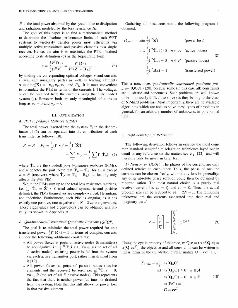
Gathering all these constraints, the following program isobtained:

Pl,min = mini

1

2iHZ′i (power loss)

s.t.1

2iHTni ≥ 0 n ∈ A (active nodes)

1

2iHTni = 0 n ∈ P (passive nodes)

1

2iHRLi = 1 (transferred power)

(8)

This a nonconvex quadratically constrained quadratic pro-gram (QCQP) [20], because some (in this case all) constraintsare quadratic and nonconvex. Such problems are well-knownto be notoriously difficult to solve (as they belong to the classof NP-hard problems). Most importantly, there are no availablealgorithms which are able to solve these types of problems ingeneral, for an arbitrary number of unknowns, in polynomialtime.

C. Tight Semidefinite Relaxation

The following derivation follows in essence the most com-mon standard semidefinite relaxation techniques layed out indetail in any reference on the matter, see e.g. [22], and willtherefore only be given in brief form.

1) Nonconvex QCQP: The phases of the currents are onlydefined relative to each other. Thus, the phase of one thecurrents can be chosen freely, without any loss in generality;any other absolute phase solution could then be obtained byrenormalization. The most natural choice is a purely realreceiver current, i.e. ir = i′r and i′′r = 0. Thus, the actualproblem size can be reduced to M = 2N − 1. The remainingunknowns are the currents (separated into their real andimaginary parts)

c =

i′ti′ri′′t

=

i′ai′pi′ri′′ai′′p

∈ RM . (9)

Using the cyclic property of the trace, cTQic = tr(cTQic) =tr(Qicc

T ), the objective and all constraints can be written inlinear terms of the (quadratic) current matrix C = ccT 0:

Pl,min = minc

tr(Q0C)

s.t. tr(QnC) ≥ 0 n ∈ Atr(QnC) = 0 n ∈ Ptr(RC) = 1

C = ccT

(10)


where

Qn =

[T′n −T′′n

T′′n T

′n

]

M×Mn = 1, ... , N (11)

Q0 =

[Z′ + RL −Z′′n

Z′′n Z′ + RL

]

M×M=

N∑

n=1

Qn (12)

R =

[RL 00 RL

]

M×M= Diag

[0N−1, RL,0N−1

](13)

The subscripts of the matrices refer to the size of the leadingprincipal submatrices thereof; the last row and column aredropped, because they would refer to the imaginary part ofthe receiver current, which is chosen to be zero at all times,as discussed.

Note that the programs (8) and (10) are mathematically fullyequivalent. The nonconvexities of the quadratic inequality andequality constraints has been isolated in the last (nonconvex)equality constraint, requiring the matrix C to be the outerproduct of the actual vector of unknowns c. All the otherconstraints are affine (or even linear) in C.

2) Semidefinite Relaxation: As for any convex relaxation,the idea is to exchange the nonconvex constraint by a con-straint that achieves almost the same — while at the sametime being convex. The constraint C = ccT is equivalentto the so-called rank-1 condition rankC = 1, which alsoimplies C 0. To obtain a convex semidefinite relaxation,the rank-1 condition is removed, while still requiring positive-semidefiniteness2 .

Thus, the following semidefinite program (SDP) is obtained:

P relaxl,min = min

Ctr(Q0C)

s.t. tr(QnC) ≥ 0 n ∈ Atr(QnC) = 0 n ∈ Ptr(RC) = 1

C 0 .

(14)

This is a convex program which can be solved reliably andefficiently using dedicated algorithms. In Matlab, it can beimplemented comfortably using CVX [23], [24] and solvedfor example using the standard solver SDPT3 [25], [26].

3) Duality: The Lagrangian, the weighted (penalized) sumof the objective and constraints [20] for this SDP (14) is givenby:

L = tr

([Q0 −

∑

n∈AλnQn −

∑

n∈PνnQn − σR

]C

)+ σ

(15a)

= tr([P− σR]C

)+ σ (15b)

= tr(QC

)− σ (15c)

where the dual variables (penalty factors) are:

2Another interpretation of C = ccT is that C − ccT = 0, equivalent tothe two semidefinite constraints C− ccT 0 and C− ccT 0. Then, therelaxation takes place by removing the second constraint and using the firstalone, by requiring the matrix of which C− ccT is the Schur complement,to be positive-semidefinite [19].

• λn ≥ 0, in order to only punish tr(QnC) < 0, ∀n ∈ A,• νn ∈ R, penalizing tr(QnC) 6= 0, ∀n ∈ P , and finally• σ ∈ R, responsible for punishing tr(RC) 6= 1.

To shorten the notation, the first two groups of dual variablesare referred to as vectors λ = [λn] and ν = [νn], respectively.

The primal problem (i.e. the original problem (14)) isobtained from the Lagrangian by minimizing the objectivewhile an inner maximization ensures that all constraints aresatisfied:

P primall,min = min

C0maxλ0ν,σ

L . (16)

Note that, if one or more of the constraints were not satisfied,the Lagrangian would be unbounded and diverge to +∞. Thus,the primal problem is (16) is really identical to (14).

The so-called dual problem is obtained by interchanging theorder of the maximization and minimization:

P duall,min = max

λ0ν,σ

minC0

L = maxλ0ν,σ

σ : Q 0 . (17)

Note that the dual program (17) takes the same form as in [19].However, some constraints on the dual variables λn ≥ 0(active transmitters) within Q have been relaxed to νn ∈ R(passive elements), thereby broadening the solution space andallowing for larger σ, meaning lower optimal PTE η.

As long as the primal problem satisfies certain conditions[20] (which are satisfied in this case, since the problem iscontinuous and convex), the dual optimum (17) is equivalentto the primal optimum (16). Therefore, in this case, the optimalsolutions of the two problems are the same, P primal

l,min = P duall,min.

4) Optimality conditions: The Karush-Kuhn-Tucker (KKT)conditions of optimality [20] for the two problems are:

C? 0 (primal feasibility) (18a)Q? 0 (dual feasibility 1) (18b)λ? 0 (dual feasibility 2) (18c)

tr(RC?) = 1 (primal equality 1) (18d)tr(QnC

?) ≥ 0 n ∈ A (primal inequalities) (18e)tr(QnC

?) = 0 n ∈ P (primal equalities) (18f)λn tr(QnC

?) = 0 n ∈ A (compl. slackness 1) (18g)tr(Q?C?) = 0 (complementary slackness 2) (18h)

The last condition, the complementary slackness, boils downto Q?C? = 0, since C?,Q? 0. In the case of rankC? = 1this also means that rankQ? = M −1, or in other words thatQ? has exactly one zero eigenvalue and c? is the correspond-ing eigenvector, the sought-after solution to the problem

5) Tightness: Since the constraints of the actual prob-lem (10) have been loosened (essentially simply by removingone of them), the optimal value of (14) is generally only alower bound on the actual optimum, i.e. P relax

l,min ≤ Pl,min.Therefore, by application of (5), the solution is only an upperbound on the maximum possible PTE, i.e. ηrelaxmax ≥ ηmax.

Equality is only achieved in the case of (14) being a tight(meaning exact) relaxation of (8) and (10). This would requirethat the removed rank constraint is naturally satisfied by therest of the problem.


To test tightness, either the eigenvalues of C? or Q? couldbe investigated, or, numerically more efficient, the (normal-ized) tightness error, defined as

ε =

∥∥C? − c?(c?)T∥∥

(c?)T c?(19)

can be used. Whenever ε is small (i.e. within the bounds oftypical numerical approximation errors of such algorithms),the semidefinite relaxation is tight and provides an exactoptimum solution c? to the nonconvex QCQP (10).

Numerical experiments showed that this seems always thecase for practical setups (typically down to ε ≈ 10−14...−10).Thus, C? has exactly one nonzero (and indeed positive)eigenvalue and c? is its corresponding eigenvector; the globaloptimum to (10).

D. Optimal Load Reactances and Voltages

The reactive loads in all passive nodes (including thereceiver) are obtained from solving the corresponding homo-geneous linear equations vp = 0 and vr = 0. Physically, thismeans that in each of these loops, the voltages across thesereactive elements are the same but with opposite sign as acrosseverything else (the unloaded WPT system), in order to net inzero voltages overall.

To this end, the unloaded voltages are calculated accordingto

v?unloaded = Zi? . (20)

Then, the optimal load reactances for the passive nodes (n ∈P) can be obtained using

x?n = −(v?unloaded,n

i?n

)′′. (21)

It can easily be verified that the zero real power flux constraintat port n, Pn = 1

2 (i?)HTni? = 1

2 (v?unloaded,ni?n)′ = 0, leads

to x?ni?n = −v?unloaded,n as required, and, thus, to zero voltage

vn = 0 at that port in the loaded case, when applying (4).

E. Optimization of the Load Resistance

The presented optimization method provides optimal cur-rents and reactive loading components, for a particular loadresistance RL. This is a very practical case; as the loadresistance is usually not free to be chosen. However, in somecases, particularly when investigating the maximum achievableperformance of the WPT in general, also the optimal loadresistance RL is of importance.

To this end, the optimal load resistance can be obtained inan outer optimization loop, as follows:

R?L = arg minRL

P relaxl,min(RL) (22)

Numerical experiments confirm the expectation, based onpractical experience with dissipation of physical multiportsystems in general, that this remaining outer optimization offinding the optimal load resistance is always convex.

Note that the optimal performance is generally not verysensitive to the load resistance [27]. Thus, for practical con-siderations, the closed-form R?L for optimal fully active MISO

configurations provided from the framework presented in [4] isusually very close to the true optimum and a simple and com-putationally efficient alternative. The calculation only requiresthe minimum-loss output impedance zo and (the square of)the mutual coupling quality factor U , both directly obtainablefrom the unloaded impedance matrix:

zo = zr − ztrZ′−1t z′tr (23)

U2 =zHtrZ

′−1t ztrz′o

(24)

R?L = z′o√

1 + U2 (25)

where the partitions are according to (1). As discussed in [27],these are the physically meaningful generalizations of the well-known SISO WPT systems [3].

IV. APPLICATION EXAMPLES

It is well understood that the region of high PTE isusually limited to electrically very short distances betweentransmitter(s) and receiver [5]. Several approaches have beenproposed in order to extend the electrical diameter of the high-PTE region, leading to the so-called “mid-range” [9] wirelesspower transfer systems. The most straightforward ideas areshielding, guiding (near-field beamforming) and focusing; allof which will be addressed briefly in the following via thethree examples depicted in Fig. 2.

y

x

z

RX

TX

Passivereflectors

RL

xr

(a)

x

y

z

RX

TX

Passiverelays

RL

xr

(b)y

x

z

RX

TX

MetasurfaceRL

xr

(c)

Fig. 2. The three principles of WPT performance enhancement under con-sideration: (a) Shielding using passive elements as reflectors, (b) guiding themagnetic near-field with passive relays [11], and (c) most general enhancementby metasurface (or -material), e.g., as proposed in [16], [17].

Note: The aim is not to thoroughly investigate each en-hancement technique, but to show the versatility of the afore-mentioned optimization technique via these three relevantnumerical examples.

A. Enhancement via Shielding by Passive Loops

One of the most straightforward ideas for WPT perfor-mance enhancement is to try to confine the magnetic fieldsto the regions between the transmitter(s) and the receiver.This is often accomplished using a ferrite shield backing thetransmitter(s) and receiver(s) in directions away from eachother [8]. However, due to the lossy nature of ferrites, theirapplication is usually restricted to the very low frequencyregions. For mobile applications also their bulkiness, weightand cost (or availability) can be an issue. Recently, using


resonant structures instead has been proposed, to reduce fieldleakage in unwanted directions [6].

The proposed test setups as shown in Fig. 3 are adoptedfrom active MISO WPT system investigations [4]: one and twoadditional transmitter loops, respectively, are placed behind thefirst transmitter (thus at greater distance to the receiver), at aconstant separation of ∆z = λ/1000, where λ is the freespacewavelength of the operating frequency f = 13.56 MHz.

y

x

z

θ

d=λ/20

(a)

y

x

z

θ

(b)

y

x

z

θ

r = λ/200

(c)

Fig. 3. The standard (reference) SISO WPT system (a) and two cases withappended passive elements: (b) the SISO-P1 with one passive and (c) theSISO-P2 with two passive elements, separated at ∆z = λ/1000. Operatingfrequency f = 13.56 MHz, wire thickness t = 5 mm.

It has been demonstrated for MISO WPT systems thatsuch constellations can outperform the standard SISO setup(a), when all transmitters are active and excited optimally.However, in this case, the additional loops are used as pas-sive elements only, meaning they do not contain any activeexcitation, but are excited via passive coupling only. Thepassive loops are shorted by (lumped) reactive elements whosereactances are then optimized using the proposed method,along with the receiver reactance, to obtain the optimallyenhanced power transfer from the transmitter (black) to thereceiver (blue). As mentioned, the load resistance RL in thereceiver could also be optimized, but since the impact on thefinal performance is usually negligible, this is omitted, here.The SISO WPT setups with one and two passive elements arecalled SISO-P1 and SISO-P2, respectively.

Fig. 4 compares the resulting maximum PTEs of the ac-tive MISO solutions (with multiple active transmitters) andthe passive configurations in all three cases, along with thetightness errors. Interestingly, the maximum achievable PTEsare very close (a); even relative differences (b) are verysmall and only noticeable at angles where power transferis difficult in general. As can be seen, similar to the activeMISO cases, adding one or two passive loops increases the

PTE from about 13% to about 21% almost 26%, respectively.Thus, adding passive loops — even at a greater distance tothe receivers — can lead to substantial enhancement of theperformance. However, when comparing the currents andpower contributions of each of the loops, as listed in Tab. I,it is observed that the optimal operating conditions for theseadditional loops lead to currents comparable to the MISOcases. Thus, when operated optimally, the additional loopsdo not act as reflectors or shielding. Instead, they seem tobe used as additional transmitters, excited passively from theremaining active transmitter, but otherwise very similar to theactive MISO case.

Lastly, as Fig. 4(c) confirms, apart from areas of generalnumerical difficulties in the angles around ±60, the tightnesserrors are in the range of 10−14 to 10−12. Thus, the relaxationis tight, meaning (14) is equivalent to the original (nonconvex)program (8) and the one true global optimum has been found.

TABLE ICURRENTS AND POWER CONTRIBUTIONS OF THE ACTIVE MISO-2/-3

SETUPS COMPARED TO THE PASSIVELY ENHANCED SISO-P1/-P2 CASES.

MISO-2 (two active TX) SISO-P1 (one passive elem.)n in (in A) Pn (in W) in (in A) Pn (in W)

1 22.6∠91.3 4.60 22.6∠91.4 12.72 22.2∠91.3 8.12 22.2∠91.3 0

Total (η = 7.86101%) 12.7 (η = 7.86100%) 12.7

(a)

MISO-3 (three active TX) SISO-P2 (two passive elem.)n in (in A) Pn (in W) in (in A) Pn (in W)

1 15.4∠91.4 1.07 15.4∠91.5 9.282 15.1∠91.4 3.03 15.1∠91.4 03 14.8∠91.4 5.18 14.8∠91.4 0

Total (η = 10.77904%) 9.28 (η = 10.77903%) 9.28

(b)

B. Enhancement via Passive Relays

Another intuitive method to enhance WPT over largerdistances is placing a passive element in-between the trans-mitter and the receiver, so that it may act as a relay, overwhich the power transfer takes place [10]. With multiplesuch relays entire relay-line-type guiding structures can be

10 20 302 = 0

!60

!30

3 = 0

30

60

!9090

SISOMISO-2MISO-3SISO-P1SISO-P2

%

(a)

!0.1 0"2/2 = !0.2

!60

!30

3 = 0

30

60

!9090

MISO-2 vs.SISO-P1MISO-3 vs.SISO-P2

(b)

!14 !12 !10 !8 !6log 0 = !16

!60

!30

3 = 0

30

60

!9090

SISO-P1SISO-P2

(c)

Fig. 4. Performance comparisons (a) of the full (active) MISO (lines) and the SISO cases with passive elements (x markers): MISO-2 vs. SISO-P1 (blue)and MISO-3 vs. SISO-P2 (red). The difference (b) is often almost unnoticeable. The tightness errors ε in (c) confirm that the relaxations in for both setups(blue SISO-P1, red SISO-P2) are equivalent to the original problems and that the global optima have been found.


constructed [11], [12] and could potentially even facilitatepower distribution over multiple paths and to multiple loads[13]–[15]. In addition to extending the high-efficiency rangeof the power transfer, relays can also help mitigate issues dueto misalignment between the transmitter and the receiver.

Both possibilities are investigated in the following example,starting off from the SISO setup as shown in Fig. 5(a): Thetransmitter and receiver (radius rtx = rrx = λ/200) are placedat either ends of a quadrant of a circle of radius r = λ/20,at the operating frequency f = 13.56 MHz. Even though theyare placed at an electrically small distance (d ≈ λ/14), themaximum achievable PTE of this system is only about 13%(b) — due to their severe misalignment.

As passive relay elements are inserted into the circular pathas shown in Fig. 5(c)-(h), the situation changes considerably;higher optimum load resistances result and the overall perfor-mance of the WPT system is enhanced considerably. As canbe seen, a single relay (c), leads to the largest performanceenhancement step: the PTE increases from 13.2% to over 60%.Interestingly, this is only about 9% under what could have beenachieved when using the passive relay as active transmitter.Thus, the passive relay setup is performing considerably betterthan a series of two SISO WPT systems of half the distance:(69.5%)2 ≈ 47.9% < 60.2%. Moreover, using the relay, theoptimum load resistance more than quadrupled. Increasing the

number of relays leads to continued performance enhance-ment, but the increase in PTE slows down. Nevertheless, fourrelays (f) lead to almost 90% PTE, ten relays are able to exceed95%. As the field plots reveal, with adding relays, the magneticfield is more and more confined to the inside of this guidingstructure, forming a bent beam from the transmitter to thereceiver and reducing the overall outside fields considerably,while the transferred power remains constant.

The graph in Fig. 6(a) shows the optimal performances vs.number of relays for different radii of the circular paths. Thepreviously mentioned rapid improvement of the performancewhen using only a small number of relays is only observed forsmall radii; at greater distances a considerably larger numberof relays is needed to achieve substantial performance en-hancement. However, even there, eventually the PTE increasessubstantially and seems to asymptotically approach a valueclose to 100%, only restrained by conduction loss of therelays. As expected, unloaded (open-connected) relays remaininvisible (solid black line), whereas shorted relays would leadto decreased PTE (dotted black line).

The graphs in Fig. 6(b) again prove that the relaxationswere tight in all cases (with tightness errors in the range of10−14 to 10−10) and that, therefore, the true global optimawere attained.

Whereas the optimization of all reactive loading elements

(a)

r=λ/20

RX

TXx

y

z

passiverelays

|B|dB

Setup

(b)

RX

TXx

y

z

SISOη = 13.3%

R?L = 0.134 Ω

(c)

RX

TXx

y

z

SISO-P1η = 60.3%

R?L = 0.79 Ω

(d)

RX

TXx

y

z

SISO-P2η = 78.2%

R?L = 1.95 Ω

(e)

RX

TXx

y

z

SISO-P3η = 85.5%

R?L = 3.78 Ω

(f)

RX

TXx

y

z

SISO-P4η = 89.1%

R?L = 5.97 Ω

(g)

RX

TXx

y

z

SISO-P7η = 93.4%

R?L = 13.3 Ω

(h)

RX

TXx

y

z

SISO-P10η = 95.2%

R?L = 20.4 Ω

Fig. 5. Comparison of some relay-enhanced WPT configurations, guiding power transfer along an arc (of radius r = λ/20). Adding relays enhances theWPT performance (max. achievable PTE) not only by constraining the fields along the arc, but also by mitigating the issue of misalignment. The performanceincrease of adding a single relay is the largest; inserting more relays improves the overall performance further and also continues to lead to larger optimalload resistances.


0 2 4 6 8 10 12 14 16 18 200

20

40

60

80

100

Number of Relays

PTE η

Number of Relays

PTE

ηin

%

r = λ/20

r = λ/10

r = λ/5relays open

relays shorted

(a)

0 2 4 6 8 10 12 14 16 18 2010

-16

10-14

10-12

10-10

10-8

Number of Relays

Norm. tightness error ε

Number of Relays

Tigh

tnes

sE

rror

ε

r = λ/20 r = λ/10 r = λ/5

(b)

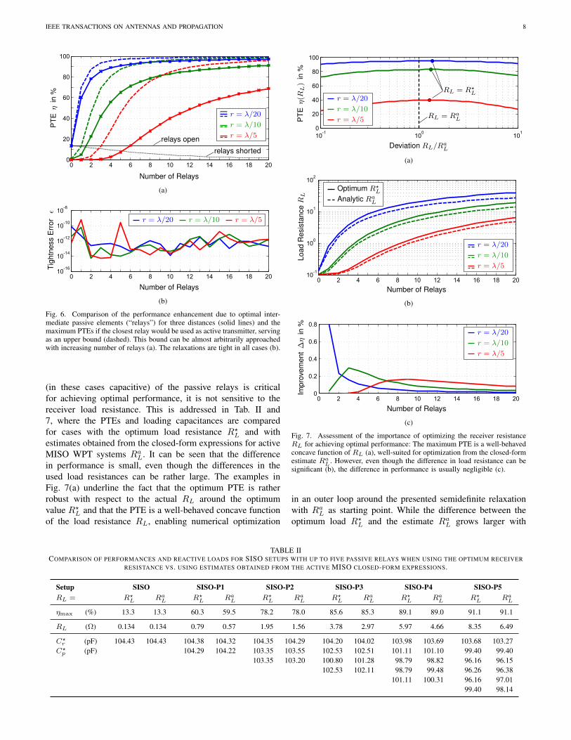
Fig. 6. Comparison of the performance enhancement due to optimal inter-mediate passive elements (“relays”) for three distances (solid lines) and themaximum PTEs if the closest relay would be used as active transmitter, servingas an upper bound (dashed). This bound can be almost arbitrarily approachedwith increasing number of relays (a). The relaxations are tight in all cases (b).

(in these cases capacitive) of the passive relays is criticalfor achieving optimal performance, it is not sensitive to thereceiver load resistance. This is addressed in Tab. II and7, where the PTEs and loading capacitances are comparedfor cases with the optimum load resistance R?L and withestimates obtained from the closed-form expressions for activeMISO WPT systems RaL. It can be seen that the differencein performance is small, even though the differences in theused load resistances can be rather large. The examples inFig. 7(a) underline the fact that the optimum PTE is ratherrobust with respect to the actual RL around the optimumvalue R?L and that the PTE is a well-behaved concave functionof the load resistance RL, enabling numerical optimization

10-1

100

101

0

20

40

60

80

100

Deviation RL/RL

a

PTE η

Deviation RL/RaL

PTE

η(R

L)

in%

RL = R?L

RL = RaL

r = λ/20

r = λ/10

r = λ/5

(a)

0 2 4 6 8 10 12 14 16 18 2010

-1

100

101

102

Number of Relays

Optim

al R

L* a

nd A

naly

tic R

L (in

Ω)

Number of RelaysLo

adR

esis

tanc

eR

L

r = λ/20

r = λ/10

r = λ/5

Optimum R?L

Analytic RaL

(b)

0 2 4 6 8 10 12 14 16 18 200

0.2

0.4

0.6

0.8

Number of Relays

PTE Improvement ∆η in %

Number of Relays

Impr

ovem

ent

∆η

in%

r = λ/20

r = λ/10

r = λ/5

(c)

Fig. 7. Assessment of the importance of optimizing the receiver resistanceRL for achieving optimal performance: The maximum PTE is a well-behavedconcave function of RL (a), well-suited for optimization from the closed-formestimate Ra

L. However, even though the difference in load resistance can besignificant (b), the difference in performance is usually negligible (c).

in an outer loop around the presented semidefinite relaxationwith RaL as starting point. While the difference between theoptimum load R?L and the estimate RaL grows larger with

TABLE IICOMPARISON OF PERFORMANCES AND REACTIVE LOADS FOR SISO SETUPS WITH UP TO FIVE PASSIVE RELAYS WHEN USING THE OPTIMUM RECEIVER

RESISTANCE VS. USING ESTIMATES OBTAINED FROM THE ACTIVE MISO CLOSED-FORM EXPRESSIONS.

Setup SISO SISO-P1 SISO-P2 SISO-P3 SISO-P4 SISO-P5RL = R?

L RaL R?

L RaL R?

L RaL R?

L RaL R?

L RaL R?

L RaL

ηmax (%) 13.3 13.3 60.3 59.5 78.2 78.0 85.6 85.3 89.1 89.0 91.1 91.1

RL (Ω) 0.134 0.134 0.79 0.57 1.95 1.56 3.78 2.97 5.97 4.66 8.35 6.49

C?r (pF) 104.43 104.43 104.38 104.32 104.35 104.29 104.20 104.02 103.98 103.69 103.68 103.27

C?p (pF) 104.29 104.22 103.35 103.55 102.53 102.51 101.11 101.10 99.40 99.40

103.35 103.20 100.80 101.28 98.79 98.82 96.16 96.15102.53 102.11 98.79 99.48 96.26 96.38

101.11 100.31 96.16 97.0199.40 98.14


an increasing number of relays, as shown in Fig. 7(b), theresulting difference in PTE is decreasing, plotted in Fig. 7(c).The resulting capacitances are in a practically realistic regionof around a hundred picofarads, with the relay capacitancesdepending more heavily on the number of relays than thereceiver reactance. Furthermore, in the case with optimumreceiver resistance R?L, the resulting capacitance values appearto always be symmetric along the guiding path.

C. Enhancement via General Metasurfaces and -MaterialsFinally, the most general form of enhancement of wireless

power transfer is considered: Enhancement by metamaterialsand metasurfaces. Such enhancements have been consideredby many research groups, see for example [16]–[18]. For sim-plicity and brevity, only an example with a metasurface (MS)will be considered; the generalization to (bulk-) metamaterialsis straightforward. Instead of using any direct methods (e.g.Huygens surface approaches using the equivalence principle)to determine the surface impedance and obtain the requiredmetasurface elements from that, the approach here is tooptimize the loading of all of the elements of a particularmetasurface with the semidefinite-relaxation based methodpresented herein.

Fig. 8 shows the setup of the metasurface-enhanced WPTexample under consideration: The transmitter and receiverloops (of diameters Dtx = Drx = λ/100) are separated bydistance d. In the middle, a 15×15-element planar loop array(loop diameters λ/500, arranged periodically at a uniformpitch of λ/200 in the x- and y-directions) is inserted, whichis referred to as metasurface. Each of the loops is loadedby a reactance (typically a capacitor Cn,m), which is to beoptimized for maximum power transfer efficiency togetherwith the receiver reactance xr. The closed-form expression(25) is used to obtain the receiver resistance RL.

y

x

z

d/2

d/2

RX

TX

15 × 15-ElementMetasurface

RLxr

λ/200

λ/500

Fig. 8. Setup of the WPT system enhanced by a passive 15×15-element loop-based metasurface (MS). Dimensions: transmitter and receiver loop diametersDtx = Drx = λ/100 (≈ 44 cm), wire thicknesses λ/2000 (≈ 2.2 cm)for transmitter and receiver and λ/104 (≈ 4.4 mm) for metasurface loops,respectively. Distance d = 0.01 ... 0.1λ (≈ 0.44 ... 4.4 m) at the operatingfrequency of f = 6.78 MHz.

This case can be optimized in straightforward manner withthe presented method. The 225 elements of the 15× 15 loopsurface in this case lead to a problem size of over 200000unknowns, since the quadratic current matrix C has (2×(225+2)− 1)2 entries. However, the problem is still solvable withina moderate computation time of a few minutes (on an Intel i3machine running CVX/SDPT3 in Matlab).

The graphs in Fig. 9(a) present the fundamental results.As reference and lower bound, the black dotted line and themarkers denote the cases without the metasurface (all elementsopen-connected) or when all metasurface loops are shorted;since the loops are electrically very small, the performancesof both of these cases are very similar. The most importantresult is the solid red line, giving the maximum achievableperformance with an optimum passive metasurface present.For comparison, the dashed red line plots the PTE of an activemetasurface, where each loop of the metasurface is connectedto a generator, serving as an upper bound on the achievableperformance.

0.02 0.04 0.06 0.08 0.10

20

40

60

80

100

max

open

short

avg

passive

worst

Distance d/λ

PTE

ηin

%

Optimum passive MSOptimum active MSMS elements open (invisible)

MS elements shortedMS uniformly loaded (3.989 nF)MS uniformly loaded (4.108 nF)

(a)

0.01 0.02 0.03 0.04 0.05 0.06 0.07 0.08 0.09 0.110

-15

10-13

10-11

Distance d/λ

Tigh

tnes

sE

rrorε

(b)

Fig. 9. Comparison of PTEs of the metasurface-enhanced WPT system: (a)Optimum active and passive PTEs (dashed and solid red, respectively), openand shorted metasurface loops (black), and two cases of uniform loading: a“good average” (blue) vs. the worst-case (green). The tightness error of theoptimum passive metasurface (b) proves tightness of the relaxation.

As can be seen, the enhancement due to the passive surfaceis significant: For example at distance d = 0.05λ, the passivesurface leads to an additional 20% in PTE over the referencecase without a metasurface. On the other hand, at the samedistance, the performance with the passive metasurface is onlyabout 10% behind that with an active metasurface.

The blue and green solid curves in Fig. 9(a) address theimportance of adequate loading of the metasurface elements.In each of these two cases, all loops of the metasurface areloaded uniformly by the same capacitance: about 3.989 nF (theoptimal center capacitance at d = 0.06λ) in the blue caseand 4.108 nF in the green case. The blue curve represents acase of good overall performance, which after some distance(about 0.04λ) is largely comparable to the optimum (solidred). The green curve represents a worst-case scenario: Usingan only slightly different capacitance value (differing by about3%), degrades the maximum overall performance far below the


case without a metasurface (the receiver reactance is optimizedto still maximize the performance using the suboptimallyloaded metasurface). Hence, the loading of the metasurfaceis absolutely crucial for optimal performance enhancement.

RX

TXx

y

z

(a)

RX

TXx

y

z

(b)

|B|dB

Fig. 10. The magnetic fields of the standard SISO system (a) and theSISO-P225 system (b), enhanced by an optimally loaded 15 × 15-elementpassive metasurface. The transmitter and receivers are located at a distanceof d = 0.08λ, while the metasurface is placed in the middle, at d/2. Themaximum achievable PTEs are about 1.2% for the reference (a) and 8.6% forthe metasurface-enhanced case (b).

The graph in Fig. 9(b) confirms that the relaxation to obtainthe maximum PTE with the passive metasurface (red solid)was tight in all cases under consideration, as the tightnesserror is in the range of 10−14 to 10−12.

Fig. 10 shows a comparison of the magnetic fields of thestandard SISO WPT system and when it is optimally enhancedby the 15 × 15-element metasurface. Since the receiver loadresistances differ very little and unit power is transferred inboth cases, the fields around the receiver loops are very similar.However, the fields around the transmitter are quite different,since in the enhanced case the efficiency was improved fromjust above 1% to about 8.6%, requiring much lower inputpower and reducing the field amplitudes accordingly.

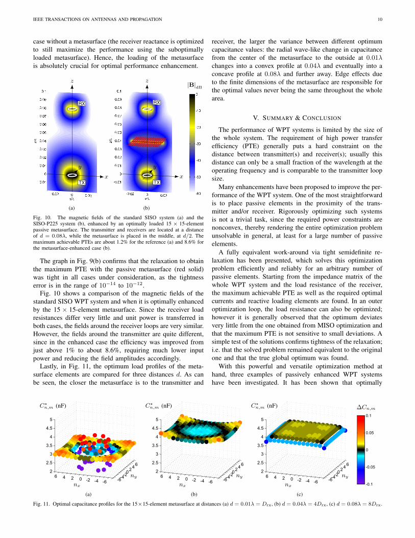
Lastly, in Fig. 11, the optimum load profiles of the meta-surface elements are compared for three distances d. As canbe seen, the closer the metasurface is to the transmitter and

receiver, the larger the variance between different optimumcapacitance values: the radial wave-like change in capacitancefrom the center of the metasurface to the outside at 0.01λchanges into a convex profile at 0.04λ and eventually into aconcave profile at 0.08λ and further away. Edge effects dueto the finite dimensions of the metasurface are responsible forthe optimal values never being the same throughout the wholearea.

V. SUMMARY & CONCLUSION

The performance of WPT systems is limited by the size ofthe whole system. The requirement of high power transferefficiency (PTE) generally puts a hard constraint on thedistance between transmitter(s) and receiver(s); usually thisdistance can only be a small fraction of the wavelength at theoperating frequency and is comparable to the transmitter loopsize.

Many enhancements have been proposed to improve the per-formance of the WPT system. One of the most straightforwardis to place passive elements in the proximity of the trans-mitter and/or receiver. Rigorously optimizing such systemsis not a trivial task, since the required power constraints arenonconvex, thereby rendering the entire optimization problemunsolvable in general, at least for a large number of passiveelements.

A fully equivalent work-around via tight semidefinite re-laxation has been presented, which solves this optimizationproblem efficiently and reliably for an arbitrary number ofpassive elements. Starting from the impedance matrix of thewhole WPT system and the load resistance of the receiver,the maximum achievable PTE as well as the required optimalcurrents and reactive loading elements are found. In an outeroptimization loop, the load resistance can also be optimized;however it is generally observed that the optimum deviatesvery little from the one obtained from MISO optimization andthat the maximum PTE is not sensitive to small deviations. Asimple test of the solutions confirms tightness of the relaxation;i.e. that the solved problem remained equivalent to the originalone and that the true global optimum was found.

With this powerful and versatile optimization method athand, three examples of passively enhanced WPT systemshave been investigated. It has been shown that optimally

-6-4-20246

-6-4-20246

2

2.5

3

3.5

4

4.5

5

d = 0.01λ

-6-4-20246

-6-4-20246

2

2.5

3

3.5

4

4.5

5

d = 0.04λ

-6-4-20246

-6-4-20246

2

2.5

3

3.5

4

4.5

5

d = 0.08λ

nx

ny

C?n,m (nF)

(a)

-6-4-20246

-6-4-20246

2

2.5

3

3.5

4

4.5

5

d = 0.01λ

-6-4-20246

-6-4-20246

2

2.5

3

3.5

4

4.5

5

d = 0.04λ

-6-4-20246

-6-4-20246

2

2.5

3

3.5

4

4.5

5

d = 0.08λ

nx

ny

C?n,m (nF)

(b)

-6-4-20246

-6-4-20246

2

2.5

3

3.5

4

4.5

5

d = 0.01λ

-6-4-20246

-6-4-20246

2

2.5

3

3.5

4

4.5

5

d = 0.04λ

-6-4-20246

-6-4-20246

2

2.5

3

3.5

4

4.5

5

d = 0.08λ

nx

ny

C?n,m (nF)

(c)

-6-4-20246

-6-4-20246

2

2.5

3

3.5

4

4.5

5

d = 0.01λ

-6-4-20246

-6-4-20246

2

2.5

3

3.5

4

4.5

5

d = 0.04λ

-6-4-20246

-6-4-20246

2

2.5

3

3.5

4

4.5

5

d = 0.08λ

-0.1

-0.05

0

0.05

0.1

∆Cn,m

Fig. 11. Optimal capacitance profiles for the 15×15-element metasurface at distances (a) d = 0.01λ = Drx, (b) d = 0.04λ = 4Drx, (c) d = 0.08λ = 8Drx.


loaded passive elements can indeed lead to substantial im-provement of the overall performance of such WPT systems.Relays can help mitigate problems of misalignment while alsoextending the region of high PTE. Multiple passive elementscan be used cooperatively, to either form transmission-linetype field guiding structures or more general structures suchas metasurfaces and metamaterials.

APPENDIX AANALYTICAL FORMULATION OF THE POSITIVE AND

NEGATIVE PIM PARTS BY EIGENVECTORS

Let the impedance matrix of the unloaded WPT system be

Z = R + jωL + jωM , (26)

where R and L are real-valued diagonal matrices containingthe losses and self-reactances (usually inductances Ln > 0, forloop-based magnetically coupled systems) of the transmittersand the receiver. M = MT is a symmetric (due to reciprocityof the passive system) hollow matrix containing the mutualimpedances jωMn,m. Generally, each Mn,m is complex-valued, due to retardation effects when the electrical distancebetween the transmitter(s) and receiver are not very small.

Moreover, let

λn,m,vn,m = eig(Tn) n = 1, ... , N (27)

denote the mth eigenvalue λn,m and corresponding eigenvec-tor vn,m of the N ×N port impedance matrix (PIM) Tn. Inthe order “negative, positive, and zero”, the eigenvalues canbe given as

λn,m =

−λ−n =1

2

(Rn −

√S2n +R2

n

)< 0 m = 1

λ+n =1

2

(Rn +

√S2n +R2

n

)> 0 m = 2

0 m = 3, ... , N(28)

where the shorthand S2n = ω2

∑m |Mn,m|2 > 0 has been

used. Note that, with these definitions, λ+n , λ−n > 0, for all n.

Finally, let the eigenvectors corresponding to the non-zeroeigenvalues be denoted by vn,m=1,2 = v∓n (omitting theindex m, as it is clear from (28) that m = 1, 2 corre-spond to the superscripts −,+, respectively) and a superscriptzero point to eigenvectors corresponding to zero eigenvalues,i.e. vn,m>2 = v0

n,m (the index m starts at 3, for theseeigenvectors). Hence, the quadratic forms with respect to theeigenvalues and eigenvectors are given by

(v±n )HTnv±n = ±λ±n · (v±n )Hv±n (29a)

vHn,mTnvn,m = 0 ∀m 6= 1, 2 . (29b)

The PIMs can be separated into their positive and negative(semidefinite) parts

Tn = T+n −T−n , (30)

where both T+n ,T

−n 0. Further, each part is simply obtained

from its eigenvalues and eigenvectors

T±n = λ±nv±n (v±n )H

(v±n )Hv±n(31)

with the denominator being the outer product and the numer-ator the inner product of the respective eigenvectors.

These eigenvectors v±n , can be obtained analytically as well:

v±n =1

M±n,N

M±n,1

...M±n,N

(32)

where M±n,m are the entries of the matrix M which is identicalto the mutual impedance matrix M, as given in (26), with theexception of the diagonal:

M±

= M± 2Diag(λ±) . (33)

Obtaining the positive and negative parts of the PIMs an-alytically, directly from the impedance matrix entries, addsboth computational efficiency as well as numerical precisionas compared to using a numerical eigenvalue decomposition.

REFERENCES

[1] A. Kurs, A. Karalis, R. Moffatt, J. D. Joannopoulos, P. Fisher, andM. Soljacic, “Wireless power transfer via strongly coupled magneticresonances,” Science, vol. 317, no. 5834, pp. 83–86, 2007.

[2] I.-J. Yoon and H. Ling, “Investigation of near-field wireless powertransfer under multiple transmitters,” IEEE Antennas Wireless Propag.Lett., vol. 10, pp. 662–665, 2011.

[3] M. Zargham and P. G. Gulak, “Maximum achievable efficiency in near-field coupled power-transfer systems,” IEEE Trans. Biomed. CircuitsSyst., vol. 6, no. 3, June 2012.

[4] H.-D. Lang, A. Ludwig, and C. D. Sarris, “Convex optimization ofwireless power transfer systems with multiple transmitters,” IEEE Trans.Antennas Propag., vol. 62, no. 9, pp. 4623–4636, September 2014.

[5] E. Waffenschmidt and T. Staring, “Limitation of inductive power transferfor consumer applications,” in 13th European Conference on PowerElecctronics and Applications, EPE, 2009.

[6] S. Kim, H. H. Park, J. Kim, J. Kim, and S. Ahn, “Design and analysisof a resonant reactive shield for a wireless power electric vehicle,” IEEETrans. Microw. Theory Tech., vol. 62, no. 4, pp. 1057–1066, April 2014.

[7] S. Li and C. C. Mi, “Wireless power transfer for electric vehicleapplications,” IEEE Trans. Emerg. Sel. Topics Power Electron., vol. 3,no. 1, pp. 4–17, March 2015.

[8] H. Kim, C. Song, D. H. Kim, D. H. Jung, I. M. Kim, Y. I. Kim, J. Kim,S. Ahn, and J. Kim, “Coil design and measurements of automotivemagnetic resonant wireless charging system for high-efficiency and lowmagnetic field leakage,” IEEE Trans. Microw. Theory Tech., vol. 64,no. 2, pp. 383–400, Feb 2016.

[9] J. S. Ho, S. Kim, and A. S. Y. Poon, “Midfield wireless powering forimplantable systems,” Proceedings of the IEEE, vol. 101, no. 6, pp.1369–1378, June 2013.

[10] F. Zhang, S. Hackworth, W. Fu, C. Li, Z. Mao, and M. Sun, “Relay effectof wireless power transfer using strongly coupled magnetic resonances,”IEEE Trans. Magn., vol. 47, no. 5, pp. 1478–1481, May 2011.

[11] M. Dionigi and M. Mongiardo, “Magnetically coupled resonant wirelesspower transmission systems with relay elements,” in 2012 IEEE MTT-SIntern. Microwave Workshop Series (IMWS), May 2012, pp. 223–226.

[12] G. Monti, L. Tarricone, M. Dionigi, and M. Mongiardo, “Magneticallycoupled resonant wireless power transmission: An artificial transmissionline approach,” in Microwave Conference (EuMC), 2012 42nd European,Oct 2012, pp. 233–236.

[13] X. Zhang, S. Ho, and W. Fu, “Quantitative design and analysis ofrelay resonators in wireless power transfer system,” IEEE Trans. Magn.,vol. 48, no. 11, pp. 4026–4029, Nov 2012.

[14] W. Zhong, C. K. Lee, and S. Hui, “Wireless power domino-resonatorsystems with noncoaxial axes and circular structures,” IEEE Trans.Power Electron., vol. 27, no. 11, pp. 4750–4762, Nov 2012.

[15] Y. Zhang, T. Lu, Z. Zhao, K. Chen, F. He, and L. Yuan, “Wireless powertransfer to multiple loads over various distances using relay resonators,”IEEE Microw. Wireless Compon. Lett., vol. 25, no. 5, pp. 337–339, May2015.


[16] Y. Urzhumov and D. R. Smith, “Metamaterial-enhanced coupling be-tween magnetic dipoles for efficient wireless power transfer,” PhysicalReview B, vol. 83, no. 20, May 2011.

[17] M. Chabalko, J. Besnoff, and D. Ricketts, “Magnetic field enhancementin wireless power using metamaterials magnetic resonant couplers.”IEEE Antennas Wireless Propag. Lett., vol. PP, no. 99, pp. 1–1, 2015.

[18] B. Wang, W. Yerazunis, and K. H. Teo, “Wireless power transfer:Metamaterials and array of coupled resonators,” Proceedings of theIEEE, vol. 101, no. 6, pp. 1359–1368, June 2013.

[19] H.-D. Lang and C. D. Sarris, “Semidefinite relaxation-based optimiza-tion of multi-transmitter wireless power transfer systems with nonconvextransmit power constraints (accepted, arxiv:1701.07344),” IEEE Trans.Microw. Theory Tech., 2016.

[20] S. Boyd and L. Vandenberghe, Convex Optimization. CambridgeUniversity Press, 12th printing, 2013.

[21] P. Triverio, S. Grivet-Talocia, M. Nakhla, F. Canavero, and R. Achar,“Stability, causality, and passivity in electrical interconnect models,”IEEE Trans. Adv. Packag., vol. 30, no. 4, pp. 795–808, Nov 2007.

[22] J. A. Taylor, Convex Optimization of Power Systems. Cambridge, UnitedKingdom: Cambridge University Press, 2015.

[23] M. Grant and S. Boyd, “CVX: Matlab software for disciplined convexprogramming, version 2.1,” http://cvxr.com/cvx, Mar. 2014.

[24] ——, “Graph implementations for nonsmooth convex programs,” inRecent Advances in Learning and Control, ser. Lecture Notes in Controland Information Sciences, V. Blondel, S. Boyd, and H. Kimura, Eds.Springer-Verlag Limited, 2008, pp. 95–110, http://stanford.edu/∼boyd/graph dcp.html.

[25] K. C. Toh, M. Todd, and R. H. Tutuncu, “SDPT3 – a matlab softwarepackage for semidefinite programming,” Optimization Methods andSoftware, vol. 11, pp. 545–581, 1999.

[26] R. H. Tutuncu, K. C. Toh, and M. J. Todd, “Solving semidefinite-quadratic-linear programs using SDPT3,” Mathematical Programming,vol. 95, pp. 189–217, 2003.

[27] H. D. Lang, A. Ludwig, and C. D. Sarris, “Optimization and designsensitivity of SISO and MISO wireless power transfer systems,” in2015 IEEE International Symposium on Antennas and Propagation &USNC/URSI National Radio Science Meeting, July 2015, pp. 406–407.

optimization of wireless power transfer systems enhanced ... · index terms convex optimization,...

Documents