optimized nurbs curve based g-code part program for cnc …
TRANSCRIPT

OPTIMIZED NURBS CURVE BASED G-CODE PART PROGRAM FOR CNC
SYSTEMS
A Thesis
Submitted to the Faculty
of
Purdue University
by
Sai Ashish Kanna
In Partial Fulfillment of the
Requirements for the Degree
of
Master of Science in Mechanical Engineering
December 2018
Purdue University
Indianapolis, Indiana

ii
THE PURDUE UNIVERSITY GRADUATE SCHOOL
STATEMENT OF COMMITTEE APPROVAL
Dr. Hazim El-Mounayri, Co-Chair
Department of Mechanical and Energy Engineering
Dr. Andres Tovar, Co-Chair
Department of Mechanical and Energy Engineering
Dr. Khosrow Nematollahi
Department of Mechanical and Energy Engineering
Dr. Jie Chen
Chair of Mechanical and Energy Engineering
Approved by:
Dr. Sohel Anwar
Chair of Graduate Program

iii
Dedicated to my family and friends.

iv
ACKNOWLEDGMENTS
I would like to thank my advisors, Dr. Tovar and Dr. El-Mounayri for their sup-
port, guidance, and motivation to better pursue my research work and constant super-
vision. Most of all, I would like to thank them for having given me the opportunity to
work under them and allowing me to use my abilities. In this journey, I have learned
many lessons from them which would help me in my future. I would like to thank
Dr. Nematollahi, member of my research committee, for his suggestions and support
that helped in improving this dissertation immensely.
I gratefully acknowledge Bishop Steering Technology, Inc for their generous grant
which helped me to pursue my research. I would like to acknowledge Jason Soungjin
Wou from Bishop Steering Technology, Inc for sharing their expertise and providing
guidance throughout.
I would like to thank the entire team of Engineering Design Research Laboratory
team and, specially, Kunal Khadhe, Kai Liu, Anahita Emami, Nishanth Bhimireddy,
and Satyajeet Shinde for their help and encouragement. At last, I would like to thank
my parents, friends and especially my sister for being their in my life and help me
reach my milestones.
v
TABLE OF CONTENTS
Page
LIST OF FIGURES . . . . . . . . . . . . . . . . . . . . . . . . . . . . . . . . . vii
ABSTRACT . . . . . . . . . . . . . . . . . . . . . . . . . . . . . . . . . . . . . xi
1 INTRODUCTION . . . . . . . . . . . . . . . . . . . . . . . . . . . . . . . . 1
1.1 Background of High Speed CNC Systems . . . . . . . . . . . . . . . . . 1
1.2 Applications on NURBS . . . . . . . . . . . . . . . . . . . . . . . . . . 3
1.3 Motivation and Objectives of this research . . . . . . . . . . . . . . . . 4
1.4 Contributions of this research . . . . . . . . . . . . . . . . . . . . . . . 5
2 DERIVATION OF NURBS . . . . . . . . . . . . . . . . . . . . . . . . . . . 6
2.1 Parametric Representation . . . . . . . . . . . . . . . . . . . . . . . . . 6
2.1.1 Parametric Cubic Polynomial Curves . . . . . . . . . . . . . . . 7
2.1.2 Boundary Conditions for Cubical Polynomial . . . . . . . . . . . 7
2.1.3 Blending Functions . . . . . . . . . . . . . . . . . . . . . . . . . 9
2.2 Curves and Surface Representation . . . . . . . . . . . . . . . . . . . . 9
2.2.1 Bezier Curves . . . . . . . . . . . . . . . . . . . . . . . . . . . . 9
2.2.2 B-Spline Curve . . . . . . . . . . . . . . . . . . . . . . . . . . . 11
2.2.3 NURBS Curve . . . . . . . . . . . . . . . . . . . . . . . . . . . 13
2.3 NURBS Formulation . . . . . . . . . . . . . . . . . . . . . . . . . . . . 15
2.4 NURBS Interpolation . . . . . . . . . . . . . . . . . . . . . . . . . . . . 24
3 METHODOLOGY TO GENERATE CNC PART PROGRAM FROM OP-TIMIZED NURBS . . . . . . . . . . . . . . . . . . . . . . . . . . . . . . . . 28
3.1 Curve Approximation . . . . . . . . . . . . . . . . . . . . . . . . . . . . 29
3.2 Parameters for Extraction of Control Points . . . . . . . . . . . . . . . 31
3.3 NURBS Parameter Optimization . . . . . . . . . . . . . . . . . . . . . 40
4 NURBS OPTIMIZATION METHODS . . . . . . . . . . . . . . . . . . . . . 43
vi
Page
4.1 Introduction . . . . . . . . . . . . . . . . . . . . . . . . . . . . . . . . . 43
4.2 Objective Function . . . . . . . . . . . . . . . . . . . . . . . . . . . . . 44
4.3 Parametric Optimization . . . . . . . . . . . . . . . . . . . . . . . . . . 45
4.4 Optimization Methods . . . . . . . . . . . . . . . . . . . . . . . . . . . 46
4.4.1 Nelder Mead Simplex Algorithm . . . . . . . . . . . . . . . . . . 46
4.4.2 Fmincon Optimization Method . . . . . . . . . . . . . . . . . . 48
4.4.3 Simulated Annealing Optimization Method . . . . . . . . . . . . 52
5 OPTIMAL NURBS FUNCTION . . . . . . . . . . . . . . . . . . . . . . . . 62
5.1 Optimized NURBS Curves . . . . . . . . . . . . . . . . . . . . . . . . 63
5.2 NURBS Curve Representation for Pinion Gear . . . . . . . . . . . . . . 69
5.3 Comparison between the Kriging Curve and NURBS Curve . . . . . . . 76
5.4 Topologically Optimized Structures using NURBS Curve . . . . . . . . 81
6 CONCLUSIONS . . . . . . . . . . . . . . . . . . . . . . . . . . . . . . . . . 86
6.1 Summary . . . . . . . . . . . . . . . . . . . . . . . . . . . . . . . . . . 86
6.1.1 Optimized NURBS Curves . . . . . . . . . . . . . . . . . . . . . 86
6.1.2 Topologically Optimized Structures using NURBS Curve . . . . 87
6.2 Original Contributions . . . . . . . . . . . . . . . . . . . . . . . . . . . 87
6.3 Future Recommendations . . . . . . . . . . . . . . . . . . . . . . . . . 88
REFERENCES . . . . . . . . . . . . . . . . . . . . . . . . . . . . . . . . . . . . 90
A Kriging Function . . . . . . . . . . . . . . . . . . . . . . . . . . . . . . . . . 94
B Matlab Code . . . . . . . . . . . . . . . . . . . . . . . . . . . . . . . . . . 100

vii
LIST OF FIGURES
Figure Page
1.1 Optimized Process workflow for CNC machining . . . . . . . . . . . . . . . 1
1.2 CNC Part Programming workflow . . . . . . . . . . . . . . . . . . . . . . . 2
2.1 Lagrange interpolation of a curve . . . . . . . . . . . . . . . . . . . . . . . 8
2.2 Hermite interpolation of a curve . . . . . . . . . . . . . . . . . . . . . . . . 8
2.3 Blending Functions . . . . . . . . . . . . . . . . . . . . . . . . . . . . . . . 9
2.4 Bezier Curve . . . . . . . . . . . . . . . . . . . . . . . . . . . . . . . . . . 10
2.5 Example of Bezier Curve . . . . . . . . . . . . . . . . . . . . . . . . . . . . 11
2.6 B-Spline Curve with degree variation . . . . . . . . . . . . . . . . . . . . . 12
2.7 Example of B-Spline Curve . . . . . . . . . . . . . . . . . . . . . . . . . . 13
2.8 NURBS Surface . . . . . . . . . . . . . . . . . . . . . . . . . . . . . . . . . 14
2.9 Block diagram of NURBS formulation . . . . . . . . . . . . . . . . . . . . 15
2.10 Control Points before variation in their position . . . . . . . . . . . . . . . 16
2.11 Control Points after variation in their position . . . . . . . . . . . . . . . . 17
2.12 NUBRS curve with weight variation . . . . . . . . . . . . . . . . . . . . . . 20
2.13 NURBS Curve with Weight Vector = 1,1,1,1,1,1,1 . . . . . . . . . . . . . . 22
2.14 NURBS Curve with Weight Vector = 1,1,1,1,1,3,1 . . . . . . . . . . . . . . 22
2.15 NURBS Curve with Weight Vector = 1,3,1,1,1,3,1 . . . . . . . . . . . . . . 23
2.16 NURBS Surface . . . . . . . . . . . . . . . . . . . . . . . . . . . . . . . . . 24
2.17 Comparison between line segment and NURBS interpolation . . . . . . . 25
2.18 NUBRS interpolation formats by different CNC makers . . . . . . . . . . 26
3.1 Block diagram for NURBS function methodology . . . . . . . . . . . . . . 28
3.2 Triangular Evaluation scheme for Basis Functions . . . . . . . . . . . . . . 34
3.3 Basis Function for order, k=2 which are straight lines . . . . . . . . . . . . 35
3.4 Basis Function for order, k=3 which are parabolic paths . . . . . . . . . . 36
viii
Figure Page
3.5 Data point plot from the periodic signal function . . . . . . . . . . . . . . 37
3.6 Plots of Data points curve (black), control points polygon (red) and ap-proximate NURBS curve (blue) . . . . . . . . . . . . . . . . . . . . . . . . 37
3.7 Error between the data points curve and the approximate curve . . . . . . 39
3.8 Truncated View of error between the data points curve and the approxi-mate curve . . . . . . . . . . . . . . . . . . . . . . . . . . . . . . . . . . . 39
3.9 Approximate NURBS curve before optimization and after optimization . . 41
4.1 Target Trident Curve . . . . . . . . . . . . . . . . . . . . . . . . . . . . . . 54
4.2 ncp=5,f ∗ = 1.8074 . . . . . . . . . . . . . . . . . . . . . . . . . . . . . . . 55
4.3 ncp=6,f ∗ = 1.8074 . . . . . . . . . . . . . . . . . . . . . . . . . . . . . . . 55
4.4 ncp=7,f ∗ = 1.2510−14 . . . . . . . . . . . . . . . . . . . . . . . . . . . . . . 56
4.5 ncp=8,f ∗ = 0.36 . . . . . . . . . . . . . . . . . . . . . . . . . . . . . . . . . 56
4.6 (a) Number of Control Points = 8 . . . . . . . . . . . . . . . . . . . . . . . 57
4.7 (b) Number of Control Points = 9 . . . . . . . . . . . . . . . . . . . . . . . 57
4.8 (c) Number of Control Points = 10 . . . . . . . . . . . . . . . . . . . . . . 58
4.9 (d) Number of Control Points = 15 . . . . . . . . . . . . . . . . . . . . . . 58
4.10 Comparison of the approximate NURBS curve before optimization andafter optimization for Periodic Signal Wave . . . . . . . . . . . . . . . . . 59
4.11 Comparison of the approximate NURBS curve before optimization andafter optimization for Star Shape. . . . . . . . . . . . . . . . . . . . . . . 60
4.12 Comparison of the approximate NURBS curve before optimization andafter optimization for Trident Curve. . . . . . . . . . . . . . . . . . . . . . 61
5.1 NURBS function block diagram . . . . . . . . . . . . . . . . . . . . . . . 62
5.2 Periodic Signal Wave using NURBS before optimization . . . . . . . . . . 63
5.3 Periodic Signal Wave using NURBS after optimization . . . . . . . . . . . 64
5.4 Error Vs Number of Control Points for Periodic Signal Wave . . . . . . . 64
5.5 Table with optimization results for Periodic Signal Wave using NURBS . . 65
5.6 Star Shape curve using NURBS before optimization . . . . . . . . . . . . 65
5.7 Star Shape curve using NURBS after optimization . . . . . . . . . . . . . 66
5.8 Error Vs Number of Control Points for Star Shape curve . . . . . . . . . . 66
ix
Figure Page
5.9 Table with optimization results for Star Shape curve using NURBS . . . . 67
5.10 Trident Curve using NURBS before optimization . . . . . . . . . . . . . . 67
5.11 Trident Curve using NURBS after optimization . . . . . . . . . . . . . . . 68
5.12 Error Vs Number of Control Points for Trident Curve . . . . . . . . . . . 68
5.13 Table with optimization results for Trident Curve using NURBS . . . . . . 69
5.14 Rack and Pinion Gears . . . . . . . . . . . . . . . . . . . . . . . . . . . . . 70
5.15 (a) Complete Involute Pinion Gear Profile . . . . . . . . . . . . . . . . . . 71
5.16 (b) Involute Gear Profile of a single tooth . . . . . . . . . . . . . . . . . . 72
5.17 (a) Involute gear profile before optimization using NURBS function . . . . 72
5.18 (b) Involute gear profile after optimization using NURBS function . . . . . 73
5.19 (c) Error Vs Number of Control Points for Involute gear profile . . . . . . 73
5.20 (d) Table with optimization results for Involute Gear Profile using NURBS 74
5.21 Table with detailed list of NURBS parameters before and after optimiza-tion for the involute gear profile. . . . . . . . . . . . . . . . . . . . . . . . 75
5.22 Comparison between Kriging and NURBS . . . . . . . . . . . . . . . . . . 77
5.23 Comparison between Kriging and NURBS . . . . . . . . . . . . . . . . . . 77
5.24 Comparison between Kriging and NURBS using subplots . . . . . . . . . . 78
5.25 Comparison between Kriging and NURBS . . . . . . . . . . . . . . . . . . 78
5.26 Surface plot of banana function . . . . . . . . . . . . . . . . . . . . . . . . 79
5.27 Surface plot of banana function using NURBS . . . . . . . . . . . . . . . 79
5.28 Contour plot of banana function . . . . . . . . . . . . . . . . . . . . . . . 80
5.29 Contour plot of banana function using NURBS . . . . . . . . . . . . . . . 80
5.30 Topology Optimized Structure . . . . . . . . . . . . . . . . . . . . . . . . . 81
5.31 (a) Topology optimized structure and (b) Topology optimized structurewith pixel values 0s and 1s . . . . . . . . . . . . . . . . . . . . . . . . . . . 82
5.32 Boundary Representation . . . . . . . . . . . . . . . . . . . . . . . . . . . 83
5.33 NURBS Curve Representation . . . . . . . . . . . . . . . . . . . . . . . . . 83
5.34 Topological optimized structure developed using 3ds software with NURBSoptimal parameters. . . . . . . . . . . . . . . . . . . . . . . . . . . . . . . 84

x
Figure Page
5.35 Topological optimized structure developed using Pro-E software with NURBSoptimal parameters . . . . . . . . . . . . . . . . . . . . . . . . . . . . . . . 85
5.36 Topological optimized structure developed using 3D printer with NURBSoptimal parameters . . . . . . . . . . . . . . . . . . . . . . . . . . . . . . . 85
A.1 Representation of curves using Kriging . . . . . . . . . . . . . . . . . . . . 94
A.2 Comparison between Kriging and NURBS using subplots . . . . . . . . . . 95
A.3 Comparison between Kriging and NURBS . . . . . . . . . . . . . . . . . . 96
A.4 Comparison between Kriging and NURBS . . . . . . . . . . . . . . . . . . 96
A.5 Comparison between Kriging and NURBS . . . . . . . . . . . . . . . . . . 97
A.6 Surface plot of banana function . . . . . . . . . . . . . . . . . . . . . . . . 97
A.7 Surface plot of banana function using NURBS . . . . . . . . . . . . . . . 98
A.8 Contour plot of banana function . . . . . . . . . . . . . . . . . . . . . . . 98
A.9 Contour plot of banana function using NURBS . . . . . . . . . . . . . . . 99

xi
ABSTRACT
Kanna, Sai Ashish. M.S.M.E., Purdue University, December 2018. OptimizedNURBS Curve Based G-Code Part Program for CNC Systems. Major Professor:Andres Tovar and Hazim El-Mounayri.
Computer Numerical Control (CNC) is widely used in many industries that needs
high speed machining of the parts with high precision, accuracy and good surface
finish. In order to avail this the generation of the CNC part program size will be
immensely big and leads to an inefficient process, which increases the delivery time
and cost of products. This work presents the automation of high-accuracy CNC tool
trajectory planning from CAD to G-code generation through optimal NURBs sur-
face approximation. The proposed optimization method finds the minimum number
of NURBS control points for a given admissible theoretical cord error between the
desired and manufactured surfaces. The result is a compact part program that is
less sensitive to data starvation than circular and spline interpolations with potential
better surface finish. The proposed approach is demonstrated with the tool path gen-
eration of an involute gear profile and a topologically optimized structure is developed
using this approach and then finally it is 3D printed.

1
1. INTRODUCTION
1.1 Background of High Speed CNC Systems
Computer Numerical Control (CNC) is widely used in high speed machining
of ultra-precision parts due to its accuracy, speed, and repeatability. The genera-
tion of CNC part programs requires a workflow that begins with the 3D model of
the part designcomputer-aided design (CAD), and it is followed by the tool path
representationcomputer-aided manufacturing (CAM), numerical control of the part
program (NC-program) via CAM post-processing (PP), workpiece manufacturing
through CNC commands, and computer-aided quality (CAQ) assurance. During the
manufacturing optimization process of a new part, the CAD-CAM-PP-CNC-CAQ
workflow needs to be repeated for each and every design iteration. This leads to an
inefficient process, which increases the delivery time and cost of new products. To
meet the demand to reduce the cost of processing of new parts, the CNC generation
time must also be reduced.
Fig. 1.1. Optimized Process workflow for CNC machining

2
Fig. 1.2. CNC Part Programming workflow
One conventional approach to reduce CNC generation time is by post-processing
the tool paths using piecewise linear (G01) and circular (G02/G03) interpolations [1].
However, this approach is of relatively low accuracy. For complex surfaces, the size of
the part program may dramatically increase with tighter tolerances (lower cord error).
Furthermore, a long part program also leads to increased storage requirements and
longer data transmission times compromising the high speed machining effectiveness.
If the part data cannot be processed fast enough, i.e., block execution time is shorter
than the block processing time, then the machine starts and stops in a machine gun
fashion causing path errors due to repeated acceleration and deceleration [2]. Even if
the data can be processed fast enough, there is always rate fluctuations and velocity
discontinuity between two consecutive line segments, which promote vibration and
reduce machining quality [1] [2] [3].
An alternative to linear and circular interpolations is the use of quadratic B-
splines (G05.1) and non-uniform rational B- splines (NURBS) (G05.2/G05.3/G06.2).
3
These approaches allow the representation of complex (free form) curves with the
promise of compact part programs. However, B-spline and NURBS interpolations are
traditionally generated from the CAM post-processing of piecewise linear segments.
While this approach increases the accuracy of the curve, it does not have a major
impact on the size of the part program.
The NURBS interpolations has been used in industries with many different ap-
proaches such as Ship Hull design, minimizing tool path fluctuation, smoothen the
feedrate for high speed machining, Optimizing Shell Structures and many more.
1.2 Applications on NURBS
This research work reconstructs a concise and accurate approximated curve or
surface of the pinion gear using the NURBS geometry. There are many optimiza-
tion methods used to minimize the error generated between the targeted curve and
the approximated curve. A new interpolation method called Adams Bashforth in-
terpolation of NURBS curve in order to realize higher precision under the condition
of satisfying speed demand [4]. A new adaptive acc-jerk-limited non-uniform ra-
tional B-spline (NURBS) interpolation method based on an optimized S-shaped C
quintic feedrate planning scheme [5].The improved quantum-behaved particle swarm
optimization (QPSO) algorithm based on NURBS is used on Ship design [6]. The
isogeometric topology optimization on NURBS Surfaces [7]. A tool path optimiza-
tion algorithm of spatial cam flank milling based on NURBS surface [8]. Recon-
struction of free-form shapes in space from their arbitrary perspective images using
NURBS [9, 10].The general bilinear transformations are used in optimizing NURBS
surfaces [11]. Optimize the control points by a web-like search algorithm [12]. An
evolutionary programming algorithm called Simulated Annealing is used to optimize
the weight and the knot by minimizing the sum square error between the fitted and
target curve and surface [13]. The optimal spatial positions and weights of a fixed
number of NURBS control points are determined using a quasi Newton optimization
4
algorithm in order to approximate a general planar target curve [14].The arrange-
ment of the knot vector and location of control points are optimized locally for every
segment of the object [15].In this research work, to obtain the NURBS curve data
an approximate curve is found based on the given data points and different opti-
mization algorithms have been implemented that are capable to identify the optimal
NURBS curve parameters. The Optimization algorithms such as SQP, Nelder-Mead,
and SA are compared in the error minimization between the approximate curve and
the target curve. One-dimensional parametric search is used to find the minimum
number of points. Lastly, the optimized data of the location of control points and
their respective weights have been used in generating the G-Codes using the NURBS
Interpolation.
1.3 Motivation and Objectives of this research
Our work adopts a less traditional but intuitive method consisting on generating
the NURBS curves directly from Cutter location(CL) data offset from a CAD model
considering constant length segments in-order to achieve continuous smooth surface
finish [16]. In this approach, the required control points, weights, and knots required
by the NURBS curves are converted directly from CL data in two steps, first we iden-
tify the constant length segments from CL data and then we implement the NURBS
interpolation to convert that into a G-code program [16–20] . While this strategy is
currently used by some high-end CNC systems such as FANUC and SIMENS [3] [21]
the technical challenge that remains unanswered is how to optimally generate the
NURBS-based part program using the minimum amount of information for a given
admissible cord error. Therefore, the objective of our work is to establish a design
approach to find the optimal location of control points and their weights with mini-
mum number of control points that lead to the most compact part program for the
required product profile and ultimately, to the highest part quality.

5
1.4 Contributions of this research
In this research we developed a NURBS function that would create the opti-
mized NURBS curve with their optimal parameters which are used in generating the
NURBS interpolation. We evaluated this function by performing some case studies
to described how this function would create the optimized NURBS curve using some
well-known geometric entities such as Periodic signal wave, star shape and Trident
curve, then we used this function to develop NURBS curve representation for pinion
gear and its comparison with different optimization methods, comparison between the
meta-models such as kriging function with NURBS representation and finally repre-
sentation of topologically optimized structures using NURBS Curve and 3D printing
their structures.

6
2. DERIVATION OF NURBS
In this chapter, we discuss briefly about how the curves are represented considering
very common methods of representing the curves such as analytical and parametric
representation of the curves. The significance of using the parametric approach over
the analytical approach is expressed. The parametric form of equations solving us-
ing the interpolation methods such as LaGrange and Hermite interpolation are well
discussed with their importance. Then the curve representation using Bezier curves,
B-Spline Curve and the most important curve representation on which this research is
based is the NURBS curve. The NURBS curve and its interpolation is well described
in this chapter with its advantages over the other curve representations.
2.1 Parametric Representation
The representation of the curves and surfaces geometric modeling can be imple-
mented by two common methods one being the classical representation of the curve
and surfaces: 1. Analytical (explicit or implicit) representation and other being the
most effective method in terms of its control over the intricate shapes: 2. Parametric
representation.
The drawbacks of analytical representation:
• The analytical representation do not offer a natural procedure to evaluate the
points on the curve or surfaces
• The representation depends on the co-ordinate system used.
• The analytical representation have no flexibility to represent intricate shapes
and to manipulate it.
7
Thus, to overcome the limitations of the analytical representation and to allow the
flexibility to control the geometric entities shapes the parametric representation have
been used. This would provide a large number of points for the geometric entities
through interpolation and they form the piecewise segments that represents entire
geometric entity with relatively simple representation.
2.1.1 Parametric Cubic Polynomial Curves
The geometric representation for 3D- modeling requires to describe the non-planar
curves, to avoid the computational difficulties and unwanted undulations that might
be introduced by higher-order polynomial curves. These requirements are satisfied by
using cubical polynomial which is the lower order polynomial that would represent
the non-planar curves. The current technology uses the polynomial representation
to represent the geometric curves and surfaces. This would establish relationship
between the coordinates and parameters.
2.1.2 Boundary Conditions for Cubical Polynomial
The boundary conditions can be described based on the geometric entity such
as a line can be define by at least two points, a parabola can be defined by three
points minimum and a cubic polynomial need at least 4 points minimum. Thus,
cubic polynomial requires four boundary conditions to describe its entity. These can
be as follows:
1. Four points that lie on the curve
2. Two points and two tangents
The equation of the cubic polynomial in the parametric form is as follows
x = a1 + b1u+ c1u2 + d1u
3 (2.1)
y = a2 + b2u+ c2u2 + d2u
3 0 ≤ u ≤ 1 (2.2)

8
z = a3 + b3u+ c3u2 + d3u
3 (2.3)
The equations above have 12 unknowns and to solve this we need to solve for 12
unknowns. This can be solved considering two methods: 1) Lagrange Interpolation
and 2) Hermite Interpolation.
Lagrange Interpolation: The fitting of the curve through points.
Fig. 2.1. Lagrange interpolation of a curve
Hermite Interpolation: The fitting of the curves through points and tangents.
Fig. 2.2. Hermite interpolation of a curve
9
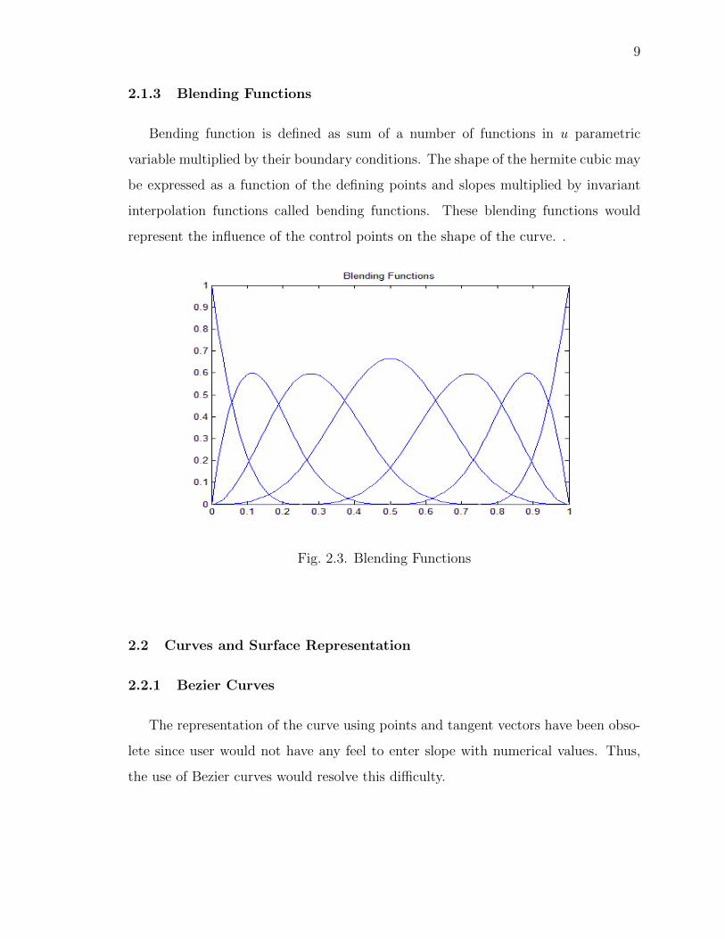
2.1.3 Blending Functions
Bending function is defined as sum of a number of functions in u parametric
variable multiplied by their boundary conditions. The shape of the hermite cubic may
be expressed as a function of the defining points and slopes multiplied by invariant
interpolation functions called bending functions. These blending functions would
represent the influence of the control points on the shape of the curve. .
Fig. 2.3. Blending Functions
2.2 Curves and Surface Representation
2.2.1 Bezier Curves
The representation of the curve using points and tangent vectors have been obso-
lete since user would not have any feel to enter slope with numerical values. Thus,
the use of Bezier curves would resolve this difficulty.
10
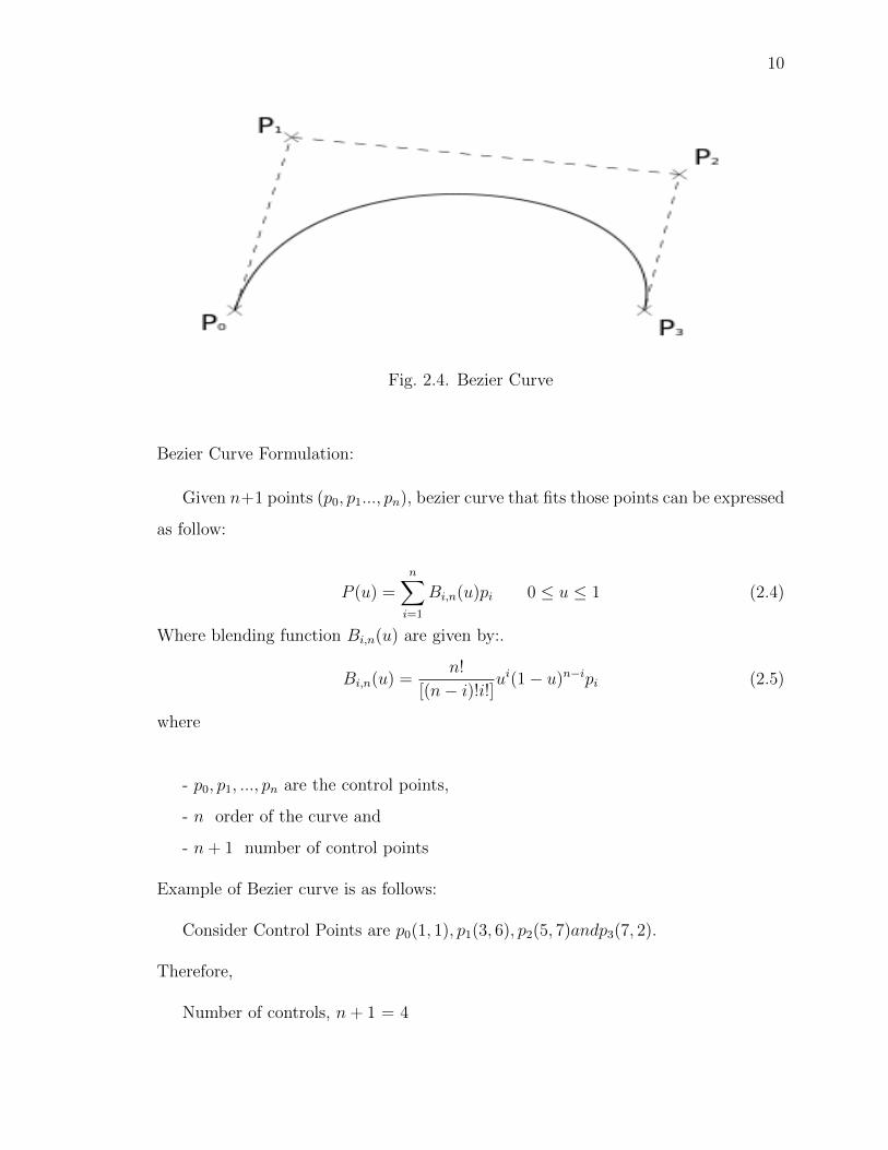
Fig. 2.4. Bezier Curve
Bezier Curve Formulation:
Given n+1 points (p0, p1..., pn), bezier curve that fits those points can be expressed
as follow:
P (u) =n∑i=1
Bi,n(u)pi 0 ≤ u ≤ 1 (2.4)
Where blending function Bi,n(u) are given by:.
Bi,n(u) =n!
[(n− i)!i!]ui(1− u)n−ipi (2.5)
where
- p0, p1, ..., pn are the control points,
- n order of the curve and
- n+ 1 number of control points
Example of Bezier curve is as follows:
Consider Control Points are p0(1, 1), p1(3, 6), p2(5, 7)andp3(7, 2).
Therefore,
Number of controls, n+ 1 = 4

11
Fig. 2.5. Example of Bezier Curve
2.2.2 B-Spline Curve
The B-spline curves are the generalization of the bezier curves and they have
unique characteristics to control or to manipulate the shape of the curve. They
provide the local control of the curve with the use of specific set of blending or basis
functions. They provide the ability to add control points without increasing its degree
of the curve.
B-Spline curve formulation:
Given n + 1 control points (p0, p1, ., pn), the B-spline curve can be expressed as
follows:
P (u) =n∑i=1
Ni,k(u)pi 0 ≤ u ≤ umax (2.6)
Where basis function Ni,k(u) are given by:
Ni,k(u) =Ni,k(u)∑ni=1Ni,k(u)
(2.7)

12
Fig. 2.6. B-Spline Curve with degree variation
Where,
Ni,1(u) =
1, if Ui ≤ Ui+1
0, otherwise
(2.8)
and where p0, p1, ., pn are the control points,
k order of the curve and
n+1 number of control points
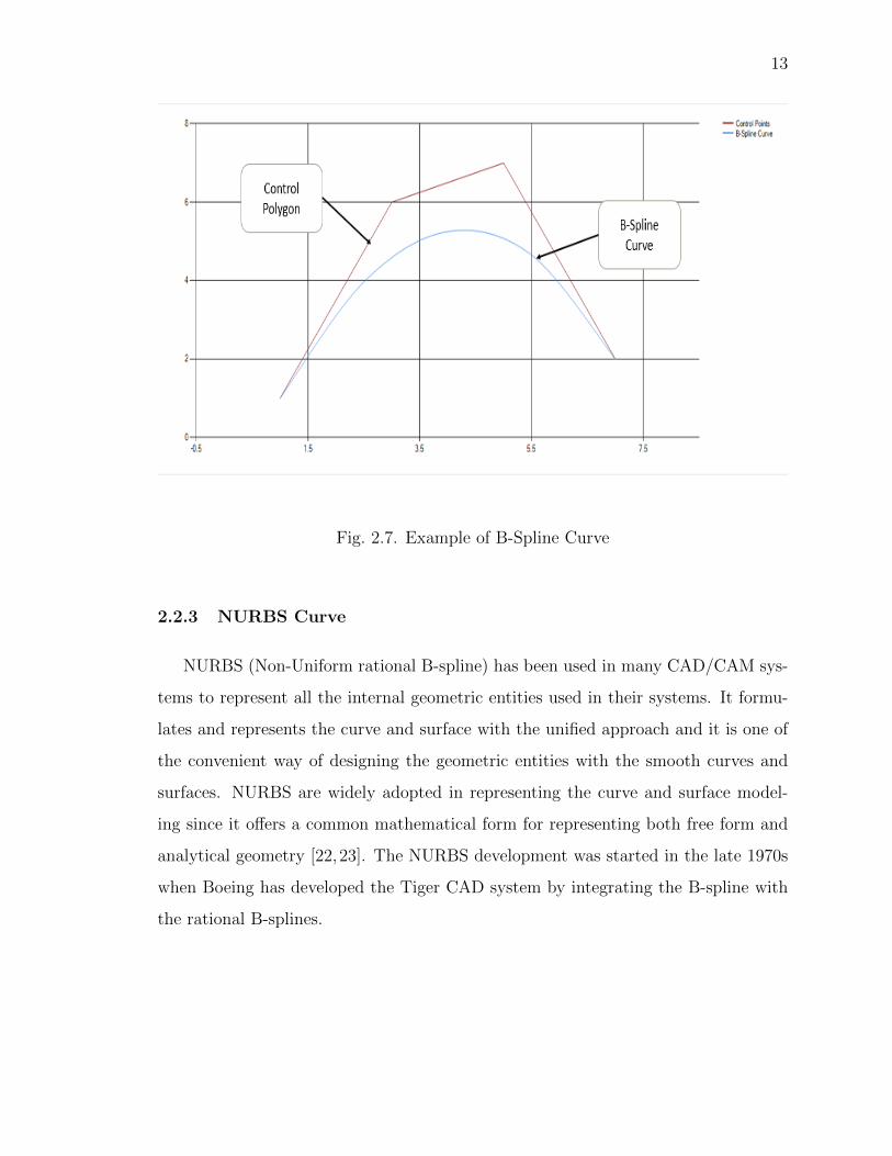
Example for B-Spline Curves is as follows:
Consider control points are p0(1, 1), p1(3, 6), p2(5, 7) and p3(7, 2).
Therefore,
- Number of control points, n+ 1 = 4,
- Order of the curve, k = 4
13
Fig. 2.7. Example of B-Spline Curve
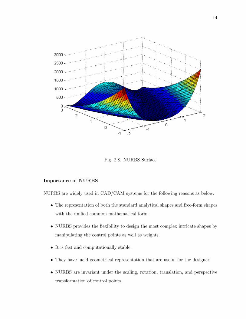
2.2.3 NURBS Curve
NURBS (Non-Uniform rational B-spline) has been used in many CAD/CAM sys-
tems to represent all the internal geometric entities used in their systems. It formu-
lates and represents the curve and surface with the unified approach and it is one of
the convenient way of designing the geometric entities with the smooth curves and
surfaces. NURBS are widely adopted in representing the curve and surface model-
ing since it offers a common mathematical form for representing both free form and
analytical geometry [22,23]. The NURBS development was started in the late 1970s
when Boeing has developed the Tiger CAD system by integrating the B-spline with
the rational B-splines.
14
Fig. 2.8. NURBS Surface
Importance of NURBS
NURBS are widely used in CAD/CAM systems for the following reasons as below:
• The representation of both the standard analytical shapes and free-form shapes
with the unified common mathematical form.
• NURBS provides the flexibility to design the most complex intricate shapes by
manipulating the control points as well as weights.
• It is fast and computationally stable.
• They have lucid geometrical representation that are useful for the designer.
• NURBS are invariant under the scaling, rotation, translation, and perspective
transformation of control points.

15
Drawbacks of NURBS
However, there are some draw backs of representing the curves and surface entities
with NURBS or any other free-form schemes.
• To represent the traditional curves and surfaces extra storage is required. For
example, to represent a full circle requires a seven control points and ten knots.
But, the traditional representation requires only the center, radius and the
normal vector to the plane of the circle.
• The curves and surfaces representation can be destroyed with the improper
implementation of weights and also can result in very bad parameterization.
2.3 NURBS Formulation
The NURBS interpolation has been widely adopted in curve and surface model-
ing since it not only offers a common mathematical form for representing free form
and analytical geometry [22, 24]. Besides its use as a mathematical description tool,
NURBS are used for CNC part programs due to its flexibility to control shape. In
this section, lets us summarize the main features of the NURBS formulation.
Fig. 2.9. Block diagram of NURBS formulation

16
Parameters of NURBS
Control Points: Control points are defined as a set of points that determine the
shape of the given profile. Figure below shows the control polygon that connect all
the control points which are represented by circles in red and the smooth blue color
curve is the required NURBS curve. The second curve below in figure is same curve,
but one of the control point is moved a bit. We can notice that entire curve has not
altered but, only at the small area near the changed control point. Thus this allows
to perform some localized changes by moving the individual control points and the
influence of the control points is rendered to the part of the curve nearest to it but,
has little or no effect to the part of the curve farther away.
.
Fig. 2.10. Control Points before variation in their position
17
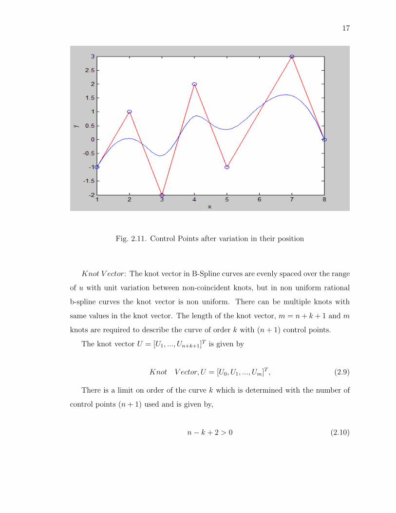
Fig. 2.11. Control Points after variation in their position
Knot V ector: The knot vector in B-Spline curves are evenly spaced over the range
of u with unit variation between non-coincident knots, but in non uniform rational
b-spline curves the knot vector is non uniform. There can be multiple knots with
same values in the knot vector. The length of the knot vector, m = n+ k + 1 and m
knots are required to describe the curve of order k with (n+ 1) control points.
The knot vector U = [U1, ..., Un+k+1]T is given by
Knot V ector, U = [U0, U1, ..., Um]T , (2.9)
There is a limit on order of the curve k which is determined with the number of
control points (n+ 1) used and is given by,
n− k + 2 > 0 (2.10)
18
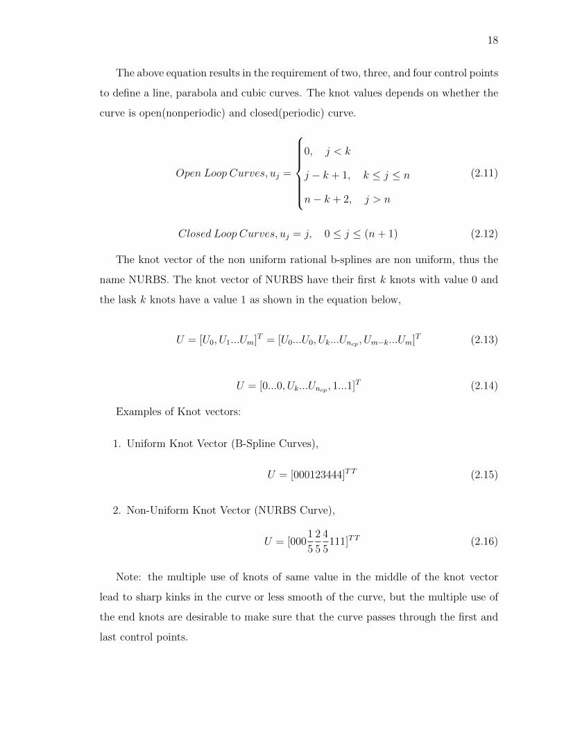
The above equation results in the requirement of two, three, and four control points
to define a line, parabola and cubic curves. The knot values depends on whether the
curve is open(nonperiodic) and closed(periodic) curve.
Open Loop Curves, uj =
0, j < k
j − k + 1, k ≤ j ≤ n
n− k + 2, j > n
(2.11)
Closed Loop Curves, uj = j, 0 ≤ j ≤ (n+ 1) (2.12)
The knot vector of the non uniform rational b-splines are non uniform, thus the
name NURBS. The knot vector of NURBS have their first k knots with value 0 and
the lask k knots have a value 1 as shown in the equation below,
U = [U0, U1...Um]T = [U0...U0, Uk...Uncp , Um−k...Um]T (2.13)
U = [0...0, Uk...Uncp , 1...1]T (2.14)
Examples of Knot vectors:
1. Uniform Knot Vector (B-Spline Curves),
U = [000123444]T T (2.15)
2. Non-Uniform Knot Vector (NURBS Curve),
U = [0001
5
2
5
4
5111]T T (2.16)
Note: the multiple use of knots of same value in the middle of the knot vector
lead to sharp kinks in the curve or less smooth of the curve, but the multiple use of
the end knots are desirable to make sure that the curve passes through the first and
last control points.

19
Basis Functions: The function Ni,k(u), that strongly determines the influence of
the control point Pi on the curve at the parametric value u is called basis function
for that control point [?]. The value of this function is a real number such as 0.5,
particular C(u) can be defined as, say 15% of one control point position, plus 40% of
another plus, so on. Thus to complete the NURBS equation we need to specify the
basis functions for each control point. It is desired that the each region of the spline
would be the average of some control points close to that region. We know that when
the moving point is far away from the control points it has influence and when it gets
closer to the control point its effect increases. Later the effect would be reduced as
the moving point passes away from control point.
Basis Function for open loop curves,
N i,k(u) =Ni,k(u)∑ncp
j=1 Nj,k(u)(2.17)
Basis Function for Closed loop curves,
Ni,k(u) = N0,k((u− i+ n+ 1)mod(n+ 1)) (2.18)
Weights: The weight vector of the NURBS curve is an effective design tool to con-
trol the NURBS curve locally and it has been implemented in many graphic software
which are being used in many industries. The values of weight vector are considered
to be positive and each control point p has a corresponding weight w. the functional-
ity of the weight in the NURBS curve is such that when the value of certain weight is
increased the curve starts moving towards the control point and similarly, when the
weight value for the corresponding control point is decreased the curve moves away
from control point. The movement of the curve with variation of the weight w at the
control point p is linear considering that the parametric variable u is constant. The
values of the weight vector are chosen by the NURBS curve designer.

20
.
Fig. 2.12. NUBRS curve with weight variation
The general form of a NURBS interpolation C(u) for a given point u is defined as
C(u) =
ncp∑i=1
Ri,k(u)Pi (2.19)
Where, Pi = [PXi, PY i]T , i = 1, , ncp contains the coordinates of the i-th control point,
ncp is the number of control points and
Ri,k(u) is the rational B-spline basis function defined as
Ri,k(u) =Ni,k(u)wi∑ncp
j=1 Nj,k(u)wj, (2.20)
Where,
N(i, k)(u) is the k − th-degree B-spline basis function and
wi is the corresponding weight.
The B-spline basis function is expressed as
Ni,1(u) =
1, Ui ≤ u < Ui+1
0, otherwise
(2.21)
21
Ni,k(u) =u− Ui
Ui+k−1 − UiNi,k−1(u) +
Ui+k − uUi+k − Ui+1
Ni+1,k−1(u), (for k > 1) (2.22)
Where,
Ui, i = 1, ..., k + ncp are the non-uniform knot values that define the knot vector U .
The knot vector U = [U1, ..., Un+k+1]T is given by
U = [0...0, Uk, ..., Uncp , 1...1]T , (2.23)
Where,
the ncp − k interior knot values are calculated as follows:
Uk = Uk−1 + ∆U = 0 + ∆U = ∆U (2.24)
Uk+1 = Uk + ∆U (2.25)
... (2.26)
Un+1 = Un + ∆U (2.27)
where,
∆U =1
(n− k + 2). (2.28)
Examples of NURBS curve is as follows:
Case 1: NURBS curve is as follows:
Control Points are p0(1,−1), p1(2, 1), p2(3,−2), p3(4, 2), p4(5,−3), p5(7, 3) and
p6(8, 0).
Therefore,
Number of control points, n+ 1 = 7,
Order of the curve k = 4
22
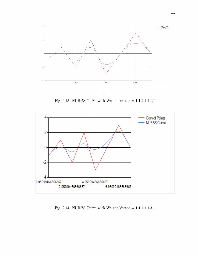
.
Fig. 2.13. NURBS Curve with Weight Vector = 1,1,1,1,1,1,1
.
Fig. 2.14. NURBS Curve with Weight Vector = 1,1,1,1,1,3,1

23
.
Fig. 2.15. NURBS Curve with Weight Vector = 1,3,1,1,1,3,1
Case 2: NURBS Surface is as follows
Control Mesh of Points:
.
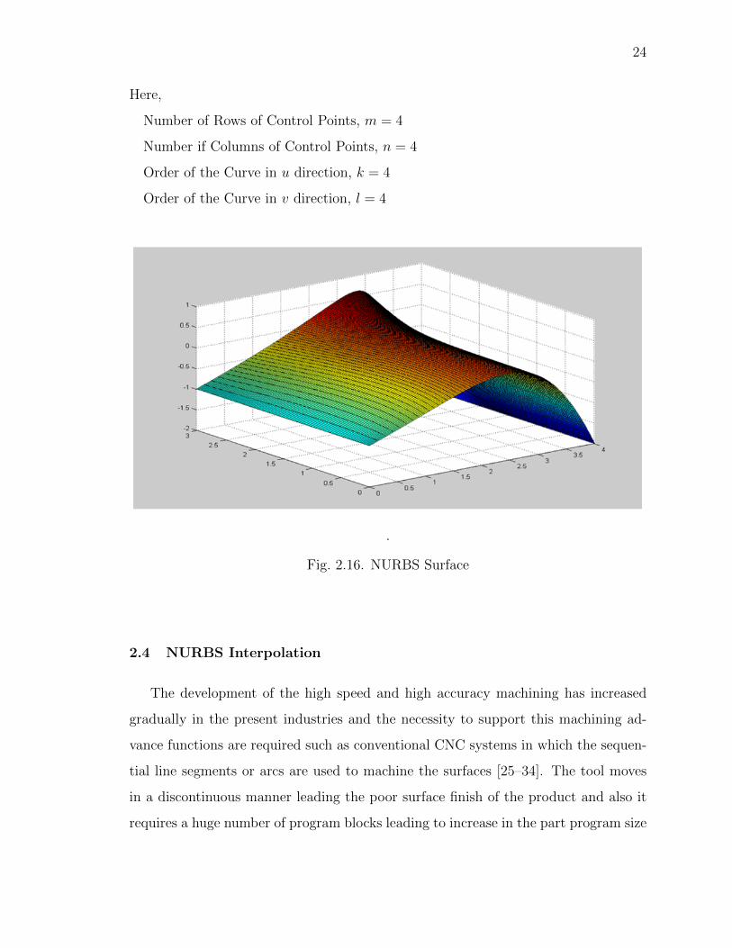
24
Here,
Number of Rows of Control Points, m = 4
Number if Columns of Control Points, n = 4
Order of the Curve in u direction, k = 4
Order of the Curve in v direction, l = 4
.
Fig. 2.16. NURBS Surface
2.4 NURBS Interpolation
The development of the high speed and high accuracy machining has increased
gradually in the present industries and the necessity to support this machining ad-
vance functions are required such as conventional CNC systems in which the sequen-
tial line segments or arcs are used to machine the surfaces [25–34]. The tool moves
in a discontinuous manner leading the poor surface finish of the product and also it
requires a huge number of program blocks leading to increase in the part program size
25
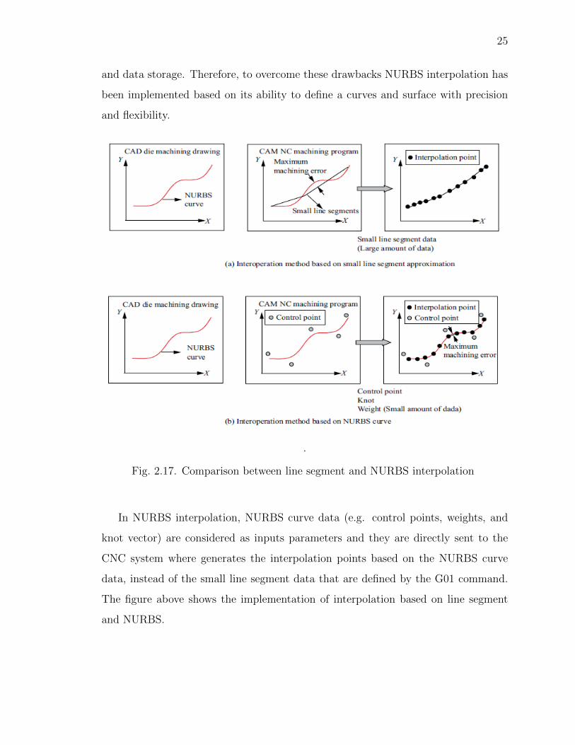
and data storage. Therefore, to overcome these drawbacks NURBS interpolation has
been implemented based on its ability to define a curves and surface with precision
and flexibility.
.
Fig. 2.17. Comparison between line segment and NURBS interpolation
In NURBS interpolation, NURBS curve data (e.g. control points, weights, and
knot vector) are considered as inputs parameters and they are directly sent to the
CNC system where generates the interpolation points based on the NURBS curve
data, instead of the small line segment data that are defined by the G01 command.
The figure above shows the implementation of interpolation based on line segment
and NURBS.
26
.
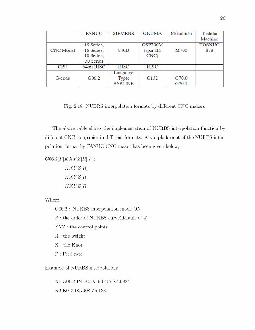
Fig. 2.18. NUBRS interpolation formats by different CNC makers
The above table shows the implementation of NURBS interpolation function by
different CNC companies in different formats. A sample format of the NURBS inter-
polation format by FANUC CNC maker has been given below,
G06.2[P ]KXY Z[R][F ];
KXY Z[R]
KXY Z[R]
KXY Z[R]
Where,
G06.2 : NURBS interpolation mode ON
P : the order of NURBS curve(default of 4)
XYZ : the control points
R : the weight
K : the Knot
F : Feed rate
Example of NURBS interpolation:
N1 G06.2 P4 K0 X19.0407 Z4.9824
N2 K0 X18.7908 Z5.1331
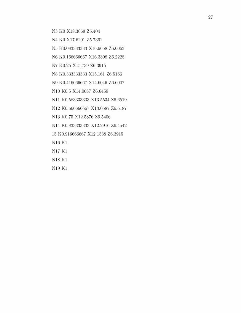
27
N3 K0 X18.3069 Z5.404
N4 K0 X17.6201 Z5.7361
N5 K0.083333333 X16.9658 Z6.0063
N6 K0.166666667 X16.3398 Z6.2228
N7 K0.25 X15.739 Z6.3915
N8 K0.333333333 X15.161 Z6.5166
N9 K0.416666667 X14.6046 Z6.6007
N10 K0.5 X14.0687 Z6.6459
N11 K0.583333333 X13.5534 Z6.6519
N12 K0.666666667 X13.0587 Z6.6187
N13 K0.75 X12.5876 Z6.5406
N14 K0.833333333 X12.2916 Z6.4542
15 K0.916666667 X12.1538 Z6.3915
N16 K1
N17 K1
N18 K1
N19 K1
28
3. METHODOLOGY TO GENERATE CNC PART
PROGRAM FROM OPTIMIZED NURBS
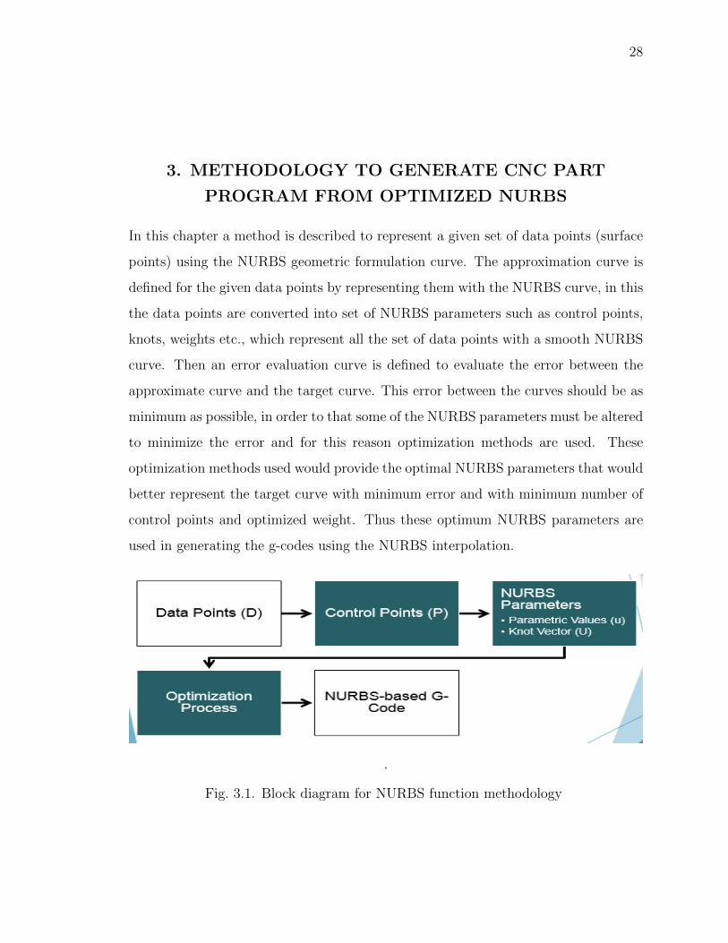
In this chapter a method is described to represent a given set of data points (surface
points) using the NURBS geometric formulation curve. The approximation curve is
defined for the given data points by representing them with the NURBS curve, in this
the data points are converted into set of NURBS parameters such as control points,
knots, weights etc., which represent all the set of data points with a smooth NURBS
curve. Then an error evaluation curve is defined to evaluate the error between the
approximate curve and the target curve. This error between the curves should be as
minimum as possible, in order to that some of the NURBS parameters must be altered
to minimize the error and for this reason optimization methods are used. These
optimization methods used would provide the optimal NURBS parameters that would
better represent the target curve with minimum error and with minimum number of
control points and optimized weight. Thus these optimum NURBS parameters are
used in generating the g-codes using the NURBS interpolation.
.
Fig. 3.1. Block diagram for NURBS function methodology

29
3.1 Curve Approximation
Curve approximation is the inverse process to point interpolation: given a set of
ndp data points Dj = [DXj, DY j]T , j = 1, ..., ndp from the target curve, the objective
is to find the ncp control points Pi = [PXi, PY i]T , i = 1, , ncp of the NURBS approx-
imation that better approximates the target curve. The approximation of a given
curve is performed in four steps:
Step 1: Parameter extraction - the parameter uj for each data point Dj is calcu-
lated using chord length parameterization. This parameter uj for each data point is
a measure of the distance of the data point along the curve. Specifically, for the ndp
data points, the parameter value at the l − th data point is given as
u1 = 0, (3.1)
ul = umax
∑ls=2 |DXs −DX,s−1|∑ndp
s=2 |DXs −DX,s−1|, (for l = 2,...,ndp) (3.2)
where DXs represent the X-coordinate of the data point Ds.
Step 2: Non-uniform knot valuesFind the knot vector U = [U1, ..., Un+k+1]T from Eqs.
(4) to (6).
Step 3: Control points - The point interpolation in Eq. (1) can be expressed in
matrix from as using data points as
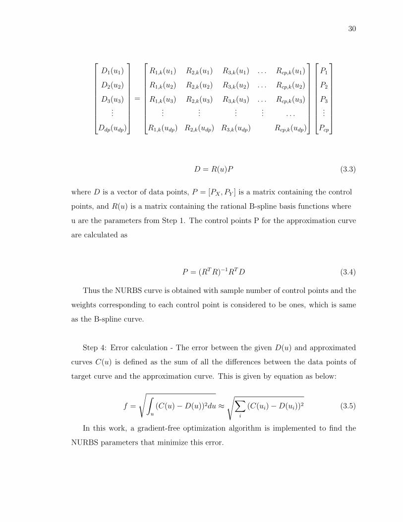
30
D1(u1)
D2(u2)
D3(u3)...
Ddp(udp)
=
R1,k(u1) R2,k(u1) R3,k(u1) . . . Rcp,k(u1)
R1,k(u2) R2,k(u2) R3,k(u2) . . . Rcp,k(u2)
R1,k(u3) R2,k(u3) R3,k(u3) . . . Rcp,k(u3)...
......
... . . .
R1,k(udp) R2,k(udp) R3,k(udp) Rcp,k(udp)
P1
P2
P3
...
Pcp
D = R(u)P (3.3)
where D is a vector of data points, P = [PX , PY ] is a matrix containing the control
points, and R(u) is a matrix containing the rational B-spline basis functions where
u are the parameters from Step 1. The control points P for the approximation curve
are calculated as
P = (RTR)−1RTD (3.4)
Thus the NURBS curve is obtained with sample number of control points and the
weights corresponding to each control point is considered to be ones, which is same
as the B-spline curve.
Step 4: Error calculation - The error between the given D(u) and approximated
curves C(u) is defined as the sum of all the differences between the data points of
target curve and the approximation curve. This is given by equation as below:
f =
√∫u
(C(u)−D(u))2du ≈√∑
i
(C(ui)−D(ui))2 (3.5)
In this work, a gradient-free optimization algorithm is implemented to find the
NURBS parameters that minimize this error.
31
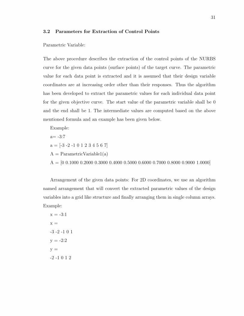
3.2 Parameters for Extraction of Control Points
Parametric Variable:
The above procedure describes the extraction of the control points of the NURBS
curve for the given data points (surface points) of the target curve. The parametric
value for each data point is extracted and it is assumed that their design variable
coordinates are at increasing order other than their responses. Thus the algorithm
has been developed to extract the parametric values for each individual data point
for the given objective curve. The start value of the parametric variable shall be 0
and the end shall be 1. The intermediate values are computed based on the above
mentioned formula and an example has been given below.
Example:
a= -3:7
a = [-3 -2 -1 0 1 2 3 4 5 6 7]
A = ParametricVariable1(a)
A = [0 0.1000 0.2000 0.3000 0.4000 0.5000 0.6000 0.7000 0.8000 0.9000 1.0000]
Arrangement of the given data points: For 2D coordinates, we use an algorithm
named arrangement that will convert the extracted parametric values of the design
variables into a grid like structure and finally arranging them in single column arrays.
Example:
x = -3:1
x =
-3 -2 -1 0 1
y = -2:2
y =
-2 -1 0 1 2

32
A = arrangement([x(:),y(:)])
ans =
-3 -2
-3 -1
-3 0
-3 1
-3 2
-2 -2
-2 -1
-2 0
-2 1
-2 2
-1 -2
-1 -1
-1 0
-1 1
-1 2
0 -2
0 -1
0 0
0 1
0 2
1 -2
1 -1
1 0
1 1
1 2

33
Knot Vector:
Compute the Knot vector assuming that there are sample number of control points
and order of the curve to be default value (say k = 4).In this algorithm we use the
non-uniform knot vector in which the first set of values till the count reached the order
of the curve value, k shall be zero and the last set of value for the count equivalent
to order of the curve shall be equal to one as shown in below example.
Example: Consider number of control points to be, n = 8 and the order of the curve
to be, k = 4.
Knot Vector = [0 0 0 0 0.2000 0.4000 0.6000 0.8000 1.0000 1.0000 1.0000 1.0000]
Computation of Basis Function:
The normalized basis functions are defined recursively as below,
Ni,1(u) =
1 ui ≤ u < ui+1
0 (otherwise)
(3.6)
Ni,k(u) =u− ui
ui+k−1 − uiNi,k−1(u) +
ui+k − uui+k − ui+1
Ni+1,k−1(u) (3.7)
Here,
u - parametric value
ui - Elements from knot vector, where ranges from i = 1 to n+ k.
Note: The size of the basis function would be of the form mxnp
Where,
m - Number of Rows in parametric variable u
np - Product of elements in Number of Control Points vector, n
For the computation of the basis functions for assumed sample number of control
points ncp we use Cox-de Boor recursion formula as mentioned above. Some of the
basis functions are calculated using the developed algorithm are shown below and if we

34
.
Fig. 3.2. Triangular Evaluation scheme for Basis Functions
observe the figure showing the basis functions with degree 1 (order, k = 2) it consists
of straight lines for all the functions in the plot. But, if we observe the basis functions
of degree 2 (order, k = 3) it consists of parabolic paths. In this recursion formula two
consecutive zero degree basis functions Ni,0 and Ni+1,0 are used to evaluate the higher
degree basis function Ni,2 and thus following the triangular evaluation scheme. This
triangular evaluation scheme is being implemented in the algorithm that has been
developed for the evaluation of the basis functions. The basis functions are validated
such that the computed basis functions shall be non-zero only in their knot span
elsewhere it should be zero as mentioned in the Cox-De door recursion formula.
Example:
N = Nfun(u(i),j,k(i),U(i,:));
Here,
u(i) = 0.5
j = 6
k(i) = 4
U ′ = [0 0 0 0 0.2000 0.4000 0.6000 0.8000 1.0000 1.0000 1.0000 1.0000]
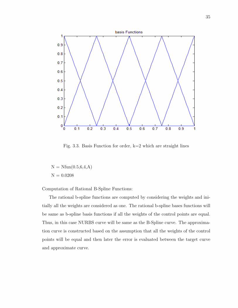
35
Fig. 3.3. Basis Function for order, k=2 which are straight lines
N = Nfun(0.5,6,4,A)
N = 0.0208
Computation of Rational B-Spline Functions:
The rational b-spline functions are computed by considering the weights and ini-
tially all the weights are considered as one. The rational b-spline bases functions will
be same as b-spline basis functions if all the weights of the control points are equal.
Thus, in this case NURBS curve will be same as the B-Spline curve. The approxima-
tion curve is constructed based on the assumption that all the weights of the control
points will be equal and then later the error is evaluated between the target curve
and approximate curve.
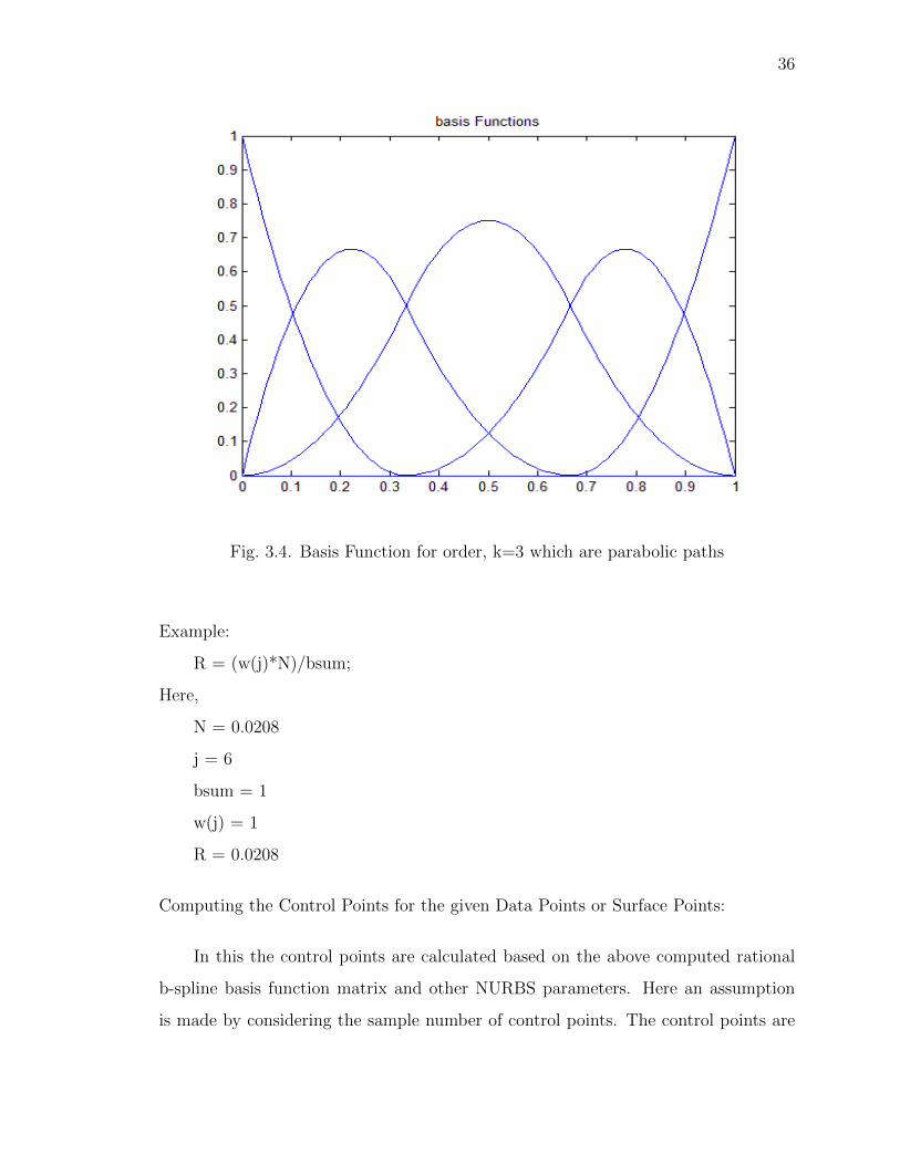
36
Fig. 3.4. Basis Function for order, k=3 which are parabolic paths
Example:
R = (w(j)*N)/bsum;
Here,
N = 0.0208
j = 6
bsum = 1
w(j) = 1
R = 0.0208
Computing the Control Points for the given Data Points or Surface Points:
In this the control points are calculated based on the above computed rational
b-spline basis function matrix and other NURBS parameters. Here an assumption
is made by considering the sample number of control points. The control points are

37
verified by checking the first and last control point of the curve and the first and last
data point of the curve are same or not. If they are similar we consider moving to the
next evaluation of error between the curves or else we revisit the above computation.
Fig. 3.5. Data point plot from the periodic signal function
The Figure shown above the representation the periodic Signal Wave function.
Here we have considered a periodic signal function from which we got our data points
or surface points.
Fig. 3.6. Plots of Data points curve (black), control points polygon(red) and approximate NURBS curve (blue)
38
Above figure shows an example how to extract the control points for the given set
of data points. The black color curve in the above figure represents the target curve.
The developed algorithm is being used to extract the given sample number of control
points and it is being represented with red in color. This curve which represents the
control points is called as the control polygon which connect all the control points.
The curve which is in blue in color is our approximate NURBS curve which nearly
represents the target curve. The shape of the curve can be altered by moving the
control points and varying the weight associated with each control point of the curve.
Error Evaluation between the curves:
Based on the above computed control points and assumed weight vector an ap-
proximate NURBS curve is constructed with the same parametric values that were
assigned to each data point of the target curve. Thus, a one to one mapping between
the target curve and approximate curve for each parametric value is obtained. The
difference between these points is calculated and their sum is evaluated as the er-
ror between the target curve and approximate curve. This error between the curves
is minimized by varying some of the NURBS parameter and to accomplish this we
consider some of the optimization methods that will reduce the error between the
curves. Thus, it provide the required NURBS curve for the given target curve and
then NURBS interpolation is applied onto it based on the optimal parameters ob-
tained after the optimization methods were applied. This optimal parameters of the
NURBS curve will be considered in generating the NURBS interpolation G Codes.
The figure below shows the error between the target curve and the approximate
curve and it is being highlighted with the red dashed lines. The summation of all the
errors between the data points curve and the approximate curve is considered to be
error that needs to be minimized in order to better represent the given target curve
using NURBS curve with minimum number of control points and with appropriate
weight associated with each control point. A truncated view of the above figure
is shown below which shows the error between the curves with better resolution.
39
Fig. 3.7. Error between the data points curve and the approximate curve
Fig. 3.8. Truncated View of error between the data points curve andthe approximate curve
Thus, this error is minimized using the optimization methods which uses the NURBS
parameters such as control points, weight vector, etc. as the constraint variables and
optimal values of these variables will better or closely represent the target curve with
minumum error.
40
3.3 NURBS Parameter Optimization
NURBS representation is very flexible and can be deformed to any intricate desired
shape required by the user. It provides enough set of parameters through which the
curve can be deformed to the desired shape. Some of the parameters that help in
achieving the desired curve shape or deformation are given below.
• Moving of the control points pi
• Increasing or decreasing the number of control points.
• Multiple locating of the control points.
• Changing the order k of the basis functions.
• Modifying the weights wi for each control point.
• Replacing the basis functions
• Rearranging the knot vector U .
• Using multiple knot values in knot vector.
• Changing the relative spacing of the knots.
In this algorithm we have considered the optimization of the NURBS curve using
the NURBS parameters such as Control points and their respective weight that would
minimize the evaluated error function to near zero and better represent the target
curve with the NURBS curve with minimum number of control points and their op-
timal weight vector associated with it. Once the optimization process is completed
as desired then the NURBS optimal parameters are used in generating the NURBS
interpolation structure as explained in the previous chapter and then the NURBS
G-Codes are implemented as required.
41
Fig. 3.9. Approximate NURBS curve before optimization and after optimization

42
The figures above show the approximate NURBS curve before optimization and
after optimization of the periodic signal function. We can observe the variation of the
control points position and their weights associated with it. Thus providing us with
the optimal NURBS parameters required in generating the NURBS interpolation of
the given product using NURBS G-Codes.

43
4. NURBS OPTIMIZATION METHODS
In this chapter optimization of the NURBS curve is done by adjusting the NURBS
parameters to optimal values so as to minimize the evaluated error function that was
calculated in the previous chapter subjected to certain constraints. The optimization
of the NURBS curve is performed using various optimization methods, such as Fmin-
con, FminSearch, Simulated Annealing and their results are shown in this chapter.
Also the NURBS Curve representation is compared with commercially available Meta
models such as Krigging function. Thus, this optimization results will be used in gen-
erating the NURBS Interpolation G-Codes with their optimal NURBS parameters.
4.1 Introduction
In the present industries the Computer Numerical Control (CNC) machining is
required with promising accuracy, speed and repeatability. Also, they are machining
the most complex products that has the complex intricate designs. This involves the
workflow CAD-CAM-PP-CNC-CAQ to manufacture a product and it has to be re-
peated. This will increase the cost of the product and delivery time. There are many
other methods that meets the requirements but they have relatively lower accuracy,
size of the part program increases which leads to increased storage requirements.
Thus, in order to reduce the time and the cost associated with its manufacturing we
have implemented a new methodology that will reduce both the time and cost using
the NURBS interpolation. This will compact the size of the part program associated
with complex product shapes and reduces delivery time. This NURBS interpolation
requires the use of optimal NURBS parameters in their G-Codes to better represent
the given product shape with NURBS Curves with the promising accuracy.
From literature it is found that many efforts have been made to optimize NURBS
44
interpolation parameters. In Chapter 1 their review and summary are clearly ex-
plained. There are many optimization methods used to minimize the error generated
between the targeted curve and the approximated curve. Some of them are Adams
Bashforth interpolation, web-like search algorithm, Simulated Annealing and quasi
Newton optimization algorithm are used to optimize the NURBS interpolation Pa-
rameters. In this research work, to obtain the NURBS curve data an approximate
curve is found based on the given data points and different optimization algorithms
have been implemented that are capable to identify the optimal NURBS curve param-
eters. The Optimization algorithms such as SQP, Nelder-Mead, and SA are compared
in the error minimization between the approximate curve and the target curve. One-
dimensional parametric search is used to find the minimum number of points. Lastly,
the optimized data of the location of control points and their respective weights have
been used in generating the G-Codes using the NURBS Interpolation.
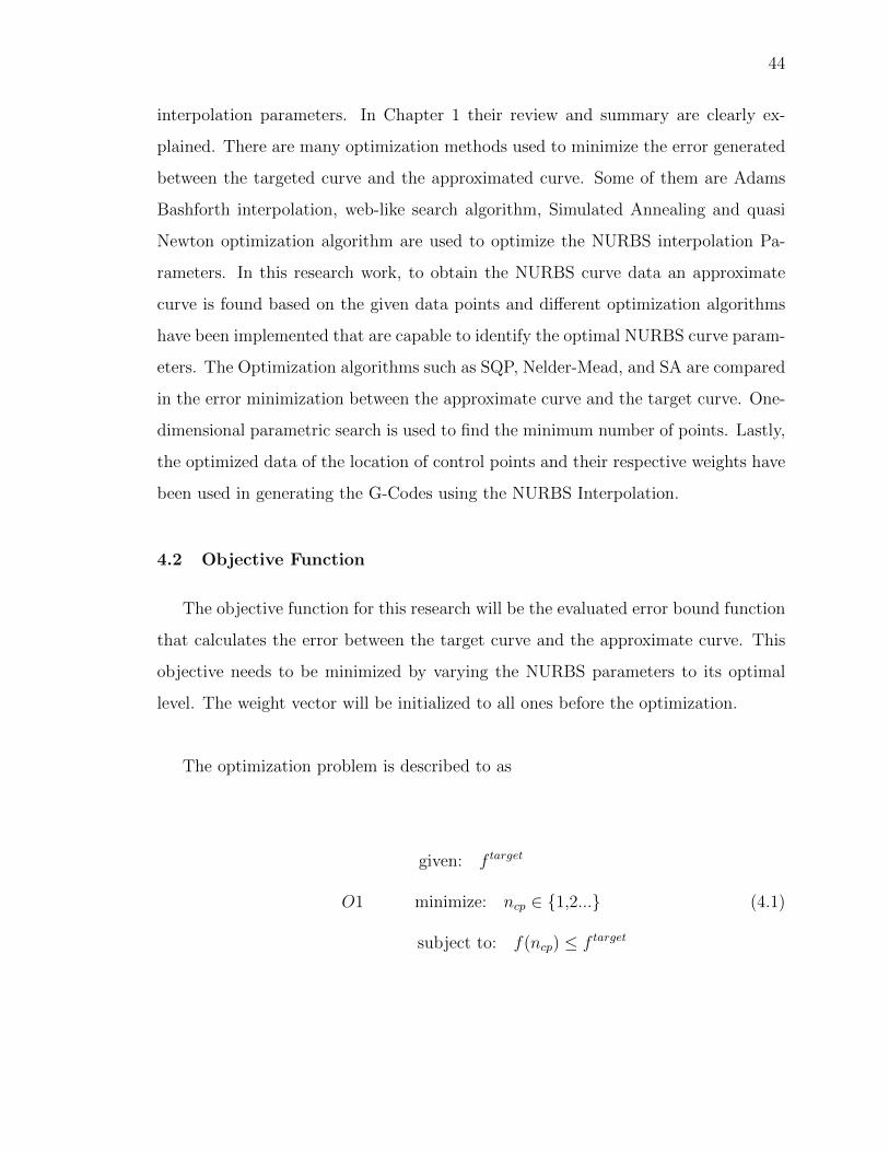
4.2 Objective Function
The objective function for this research will be the evaluated error bound function
that calculates the error between the target curve and the approximate curve. This
objective needs to be minimized by varying the NURBS parameters to its optimal
level. The weight vector will be initialized to all ones before the optimization.
The optimization problem is described to as
given: f target
O1 minimize: ncp ∈ {1,2...} (4.1)
subject to: f(ncp) ≤ f target
45
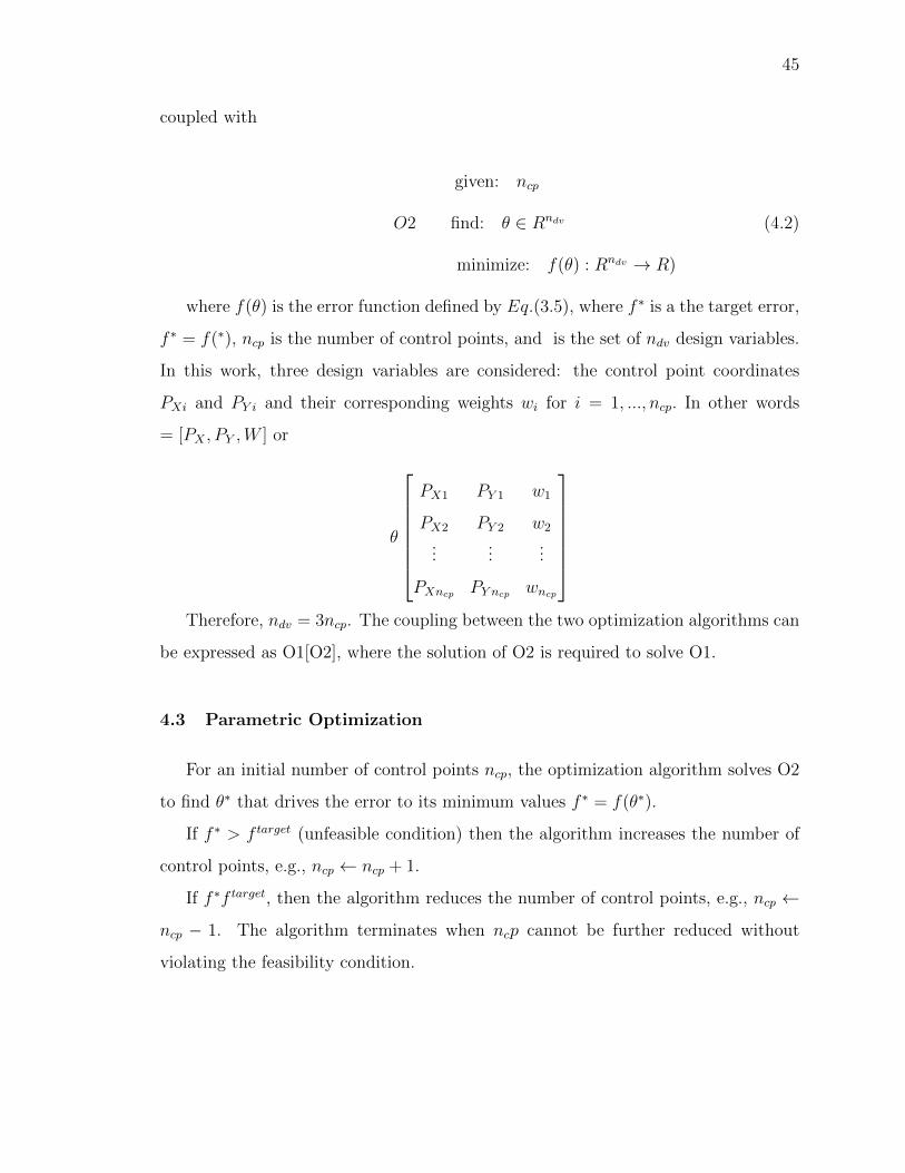
coupled with
given: ncp
O2 find: θ ∈ Rndv (4.2)
minimize: f(θ) : Rndv → R)
where f(θ) is the error function defined by Eq.(3.5), where f ∗ is a the target error,
f ∗ = f(∗), ncp is the number of control points, and is the set of ndv design variables.
In this work, three design variables are considered: the control point coordinates
PXi and PY i and their corresponding weights wi for i = 1, ..., ncp. In other words
= [PX , PY ,W ] or
θ
PX1 PY 1 w1
PX2 PY 2 w2
......
...
PXncp PY ncp wncp
Therefore, ndv = 3ncp. The coupling between the two optimization algorithms can
be expressed as O1[O2], where the solution of O2 is required to solve O1.
4.3 Parametric Optimization
For an initial number of control points ncp, the optimization algorithm solves O2
to find θ∗ that drives the error to its minimum values f ∗ = f(θ∗).
If f ∗ > f target (unfeasible condition) then the algorithm increases the number of
control points, e.g., ncp ← ncp + 1.
If f ∗f target, then the algorithm reduces the number of control points, e.g., ncp ←
ncp − 1. The algorithm terminates when ncp cannot be further reduced without
violating the feasibility condition.
46
The calculation of f ∗ requires the solution of O2. In this paper NelderMead
algorithm, Sequential Quadratic Programming Algorithm and Simulated Annealing
Optimization Methods are used to solve the optimization problem O2.
4.4 Optimization Methods
4.4.1 Nelder Mead Simplex Algorithm
The Nelder-Mead (NM) simplex algorithm is one of the most used gradient-free
search method for solving the unconstrained optimization problems [35,36]. A simplex
is a geometric gure in ndv dimensions that is the convex hull of ndv+1 vertices identified
as 1, 2, ..., (ndv+1). The vertices are ordered according to the objective function values
f(θ1) ≤ f(θ2)... ≤ f(θnnd+1), (4.3)
where θ1 is referred to as the best vertex and to θndv+1 to as the worst vertex.
Lagarias et al. [13] provide tie-breaking rules such as those given in are required for
the method when two vertices have the same objective value.
The NM algorithm uses four operations: reection, expansion, contraction, and shrink,
each being associated with a scalar parameter: α (reflection), β (expansion), γ (con-
traction), and δ (shrink). The values of these parameters satisfy α > 0, β > 1,
0 < γ < 1, and 0 < δ < 1. In the standard implementation of the NM method, the
parameters are chosen to be {α, β, γ, δ} = {1, 2, 1/2, 1/2}. We now outline the NM
algorithm as follows [13]:
Step 1: Sort - Evaluate f at the ndv + 1 vertices of and sort the vertices.
Step 2. Reflection - Let θ be the centroid of the ndv best vertices. Compute the
reection point r from
47
θr = θ + α(θ − θndv+1). (4.4)
The evaluate
fr = f(θr) (4.5)
If f1 ≤ fr < fndvthen replace θndv+1 with θr.
Step 3: Expansion - If fr < f1 then compute the expansion pointθe from
θe = θ + β(θr − θ). (4.6)
and evaluate fe = f(θe). If fe < fr then replace θndv+1 with θe, otherwise replace
θndv+1 with θr.
Step 4: Outside contraction - If fn ≤ fr < fn+1, compute the outside contraction
point
θoc = θ + γ(θr − θ) (4.7)
and evaluate foc = f(θoc). If foc ≤ f r then replace θndv+1 with θoc, otherwise go
to Step 6.
Step 5: Inside contraction - If f r > fndv+1 then compute the inside contraction
point θic from
θic = θ − γ(θr − θ) (4.8)
and evaluate fic = f(ic). If fic < fndv+1 then replace θndv+1 with θic, otherwise go
to Step 6.
48
Step 6. Shrink - Calculate the ndv vertices
θi = θ1 + δ(θi − θ1) (4.9)
and calculate fi = f(θi) for 2 ≤ ndv + 1.
Step 7: Termination criteria - The vertices of the simplex at the next iteration
are θ1, ..., θndv+1. Finally, verify termination criteria,
|f1 − fndv+1| ≤ εf (4.10)
and
|θ1 − θndv+1| ≤ εθ (4.11)
where εf and εθ are small numbers, εf = εθ = 10−6. If the algorithm is terminated
then the optimizer is θ1 with the minimum value f1. To demonstrate the proposed
optimization method, let us consider the manufacturing of a precise rack and pinion
gear.
4.4.2 Fmincon Optimization Method
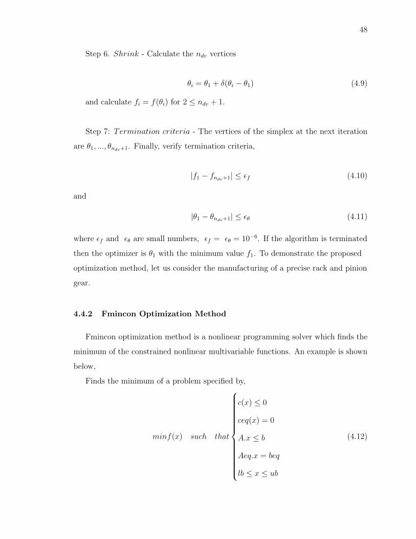
Fmincon optimization method is a nonlinear programming solver which finds the
minimum of the constrained nonlinear multivariable functions. An example is shown
below,
Finds the minimum of a problem specified by,
minf(x) such that
c(x) ≤ 0
ceq(x) = 0
A.x ≤ b
Aeq.x = beq
lb ≤ x ≤ ub
(4.12)

49
Here,
- b and beq are vectors,
- A and Aeq are matrices,
- c(x) and ceq(x) are functions that returns vectors
- f(x) is a function that returns scalar
- f(x), c(x) and ceq(x) can be nonlinear functions.
The algorithms used in solving these constrained nonlinear functions are:
1. Interior-point optimization
2. SQP Optimization
3. Active-Set Optimization
4. Trust-Region-Reflective Optimization
Interior Point Algorithm:
The interior point algorithm uses a sequence of approximate problems to solve
the constrained nonlinear minimization function. The original problem is defined as
below,
minf(x), subject to h(x) = 0 and g(x) ≤ 0, (4.13)
For each µ < 0, the approximate problem is,
minfµ(x, s) = minf(x)− µ∑i
ln(si), subject to h(x) = 0 and g(x) + s = 0,
(4.14)
There are as many slack variables si as there are inequality constraints g. The
si are restricted to be positive to keep ln(si) bounded. As µ decreases to zero, the
minimum of fµ should approach the minimum of f . The added logarithmic term is
called a barrier function.

50
To solve the approximate problem, the algorithm uses one of two main types of
steps at each iteration:
- A direct step in (x, s). This step attempts to solve the KKT equations
- A CG (conjugate gradient) step, using a trust region.
By default, the algorithm first attempts to take a direct step. If it cannot, it
attempts a CG step. One case where it does not take a direct step is when the
approximate problem is not locally convex near the current iterate
At each iteration the algorithm decreases a merit function, such as
minf(x, s) + v||(h(x), g(x) + s)||. (4.15)
The parameter may increase with iteration number in order to force the solution
towards feasibility. If an attempted step does not decrease the merit function, the
algorithm rejects the attempted step, and attempts a new step. If either the objective
function or a nonlinear constraint function returns a complex value, NaN, Inf, or an
error at an iterate xj, the algorithm rejects x + j. The rejection has the same effect
as if the merit function did not decrease sufficiently: the algorithm then attempts a
different, shorter step.
Active Set Optimization Algorithm:
The active set optimization is a constrained optimization method that transforms
the given problem into an easier sub problem that can be solved based on the iterative
process. In the early methods large class constrained problems are transformed into
unconstrained problems using a penalty function for the given constraints considering
their constraint boundaries. Now these methods are considered to be inefficient and
these methods are replaced with the use of Karush Kuhn Tucker (KKT) equations.
These KKT equations are necessary to find the optimality of the given constrained
optimization problem and if the given problem is convex programming problem and
the constraints are convex function then the KKT equation are sufficient enough to
get the global solution point for the given constrained optimization problem.

51
∇f(x∗) +m∑i=1
λi.∇Gi(x∗) = 0 (4.16)
λi.Gi(x∗) = 0, i = 1, ..,me (4.17)
λi ≥ 0, i = me + 1, . . . .,m, (4.18)
The above equation shows that the gradients between the objective function and
the active constraints are removed at their solution point. The gradients are replaced
with the LaGrange multipliers (i, i = 1, 2m) that would balance the deviation of
the magnitude of the objective function and constraint gradients. In this operation
only the active constraints are considered and all the other non-active constraints are
multiplied by Lagrange multiplieri = 0. Thus the solution of the KKT equations is
considered to be the bases for many nonlinear constrained optimization problems.
The Lagrange multipliers are computed directly with the use of algorithms such as
quasi-newton methods.
Sequential Quadratic Programming Algorithm:
The sequential quadratic programming algorithms is similar to the act set
optimization algorithm but the only different between them is as below:
1. Strict Feasibility with respect to Bounds
2. Robustness to Non-Double Results
3. Refactored Linear Algebra Routines
4. Reformulated Feasibility Routines
Trust-Region Methods for Nonlinear Minimization:
To understand the trust-region approach to optimization, consider the uncon-
strained minimization problem, minimize f(x), where the function takes vector ar-
guments and returns scalars. Suppose you are at a point x in n-space and you want

52
to improve, i.e., move to a point with a lower function value. The basic idea is to
approximate f with a simpler function q, which reasonably reflects the behavior of
function f in a neighborhood N around the point x. This neighborhood is the trust
region. A trial step s is computed by minimizing (or approximately minimizing) over
N . This is the trust-region subproblem,
min{q(s), s ∈ N}, (4.19)
The current point is updated to be x + s if f(x + s) < f(x); otherwise, the current
point remains unchanged and N , the region of trust, is shrunk and the trial step
computation is repeated.
4.4.3 Simulated Annealing Optimization Method
The Simulated annealing optimization methods is used where the number of ob-
jects increase for certain optimization problem which cannot be solved by other meth-
ods. It is a very practical algorithm as the name indicate the process of heating the
metal and then cooling it slowly. This method would provide with a very good solu-
tion even in the presence of noisy data unlikely with the optimal solution. An example
for this methods is a traveling salesman who visits many cities with minimizing the
total travel mileage. Suppose if the salesman started his travel with a random ticket
and has planned to reduce his total travel mileage in the upcoming travel at each
exchange. This approach will provide the local minimum but not the Global mini-
mum as required. The simulated annealing has improved this with the inclusion of
two algorithms. The first being the metropolis algorithm that includes some trades
that do not reduce the total mileage to allow the solver to have extra space for its
solution. These bad trades are allowed with the formula indicated below,
e−∆D/T > R(0, 1), (4.20)
Where,
53
- is the change of distance implied by the trade (negative for a ”good” trade; positive
for a ”bad” trade),
- is a ”synthetic temperature,” and
- is a random number in the interval .
- is called a ”cost function,” and corresponds to the free energy in the case of anneal-
ing a metal
The space for solution can be increased with the inclusion of bad trades and this
can be possible if the T is larger.
The second methods uses the process of annealing to lower the temperature and
it would restrict the size of the allowed bad trades. This is done because after making
many trades we observe that the cost function is reduced very slowly and that is the
reason we lower the temperature in order to restrict the size of the allowed bad trades.
This is done periodically many times and then it starts to accept only the good trades
that provides us with the local minimum of the cost function. There is another meth-
ods that is faster than the rest of the two and it is based on how the temperature is
reduced in annealing process. In this method they use the threshold acceptance which
will allow the bad trades to be included in the space of solution up to the level of
threshold mark and this threshold is decreased periodically. Thus, this will eliminate
the use of exponentiation and random number computation in the Boltzmann criteria.
Some of the observations before optimization and after optimization of the gen-
erated approximate NURBS curve are shown below. For this observation we have
considered some of the well know geometric entities such as periodic signal wave, star
shape and trident curve. We have shown an example below using the periodic signal
wave, the nature how the number of control points are very important in generating
the approximate NURBS curve which is close enough to represent the target curve.
After the selection of the sample number of control points for the approximate curve
54
which is close enough to target curve, we then optimize the weight vector of the
NURBS approximate curve using the above optimization methods and some of the
examples are shown below.
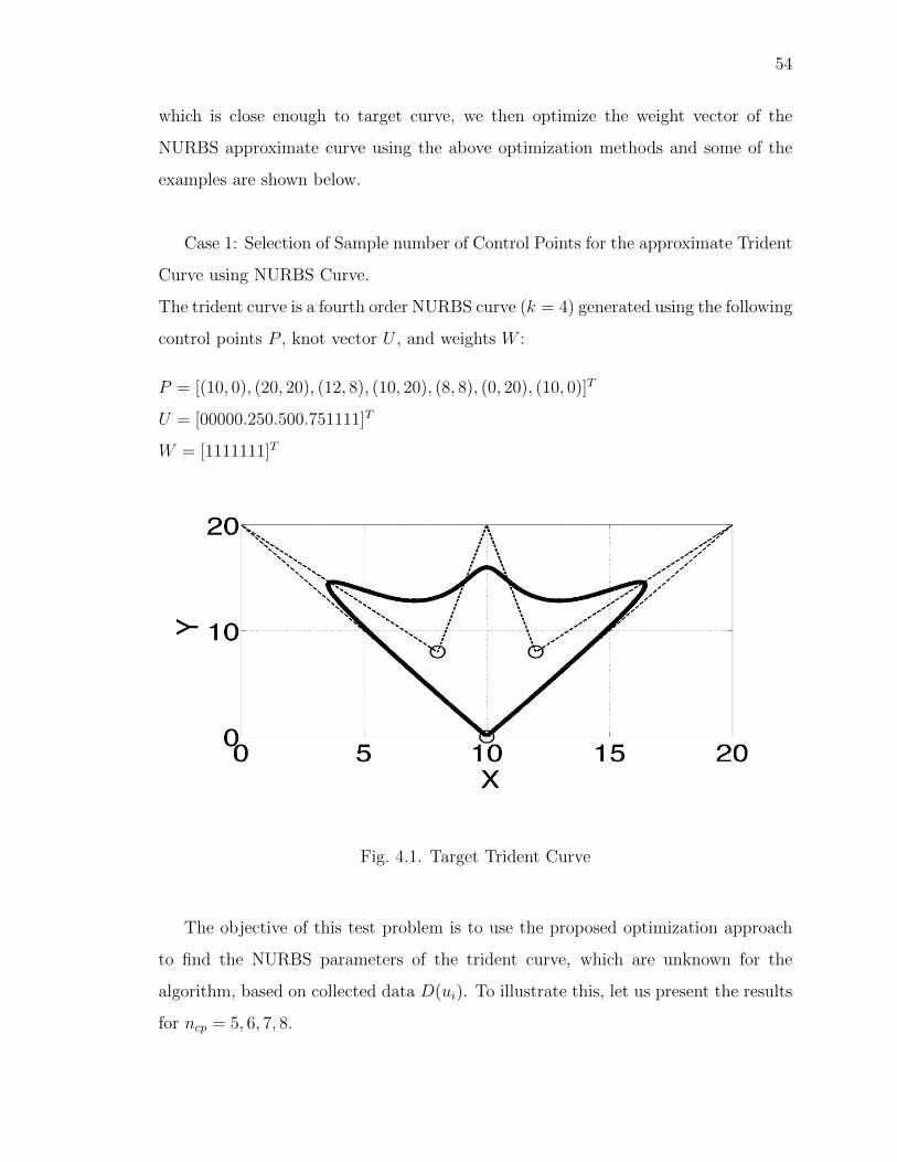
Case 1: Selection of Sample number of Control Points for the approximate Trident
Curve using NURBS Curve.
The trident curve is a fourth order NURBS curve (k = 4) generated using the following
control points P , knot vector U , and weights W :
P = [(10, 0), (20, 20), (12, 8), (10, 20), (8, 8), (0, 20), (10, 0)]T
U = [00000.250.500.751111]T
W = [1111111]T
Fig. 4.1. Target Trident Curve
The objective of this test problem is to use the proposed optimization approach
to find the NURBS parameters of the trident curve, which are unknown for the
algorithm, based on collected data D(ui). To illustrate this, let us present the results
for ncp = 5, 6, 7, 8.
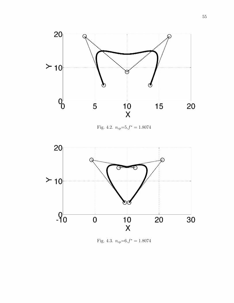
55
Fig. 4.2. ncp=5,f ∗ = 1.8074
Fig. 4.3. ncp=6,f ∗ = 1.8074

56
Fig. 4.4. ncp=7,f ∗ = 1.2510−14
Fig. 4.5. ncp=8,f ∗ = 0.36

57
Case 2: Selection of Sample number of Control Points for the approximate Periodic
Signal Wave NURBS Curve
Fig. 4.6. (a) Number of Control Points = 8
Fig. 4.7. (b) Number of Control Points = 9

58
Fig. 4.8. (c) Number of Control Points = 10
Fig. 4.9. (d) Number of Control Points = 15
59
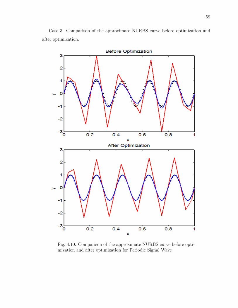
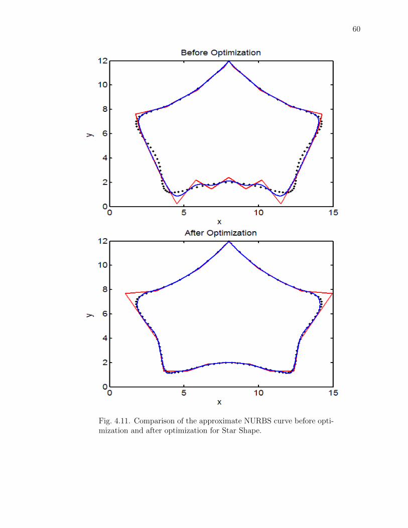
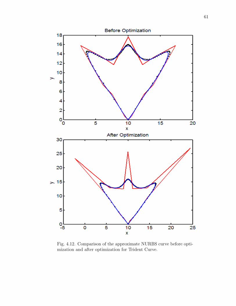
Case 3: Comparison of the approximate NURBS curve before optimization and
after optimization.
Fig. 4.10. Comparison of the approximate NURBS curve before opti-mization and after optimization for Periodic Signal Wave
60
Fig. 4.11. Comparison of the approximate NURBS curve before opti-mization and after optimization for Star Shape.
61
Fig. 4.12. Comparison of the approximate NURBS curve before opti-mization and after optimization for Trident Curve.

62
5. OPTIMAL NURBS FUNCTION
In this chapter the developed NURBS function is described with some applications.
These applications would follow the methodology described in the previous chapters
and the optimized NURBS curve with their optimal parameters are used in generating
the NURBS interpolation. Some of the case studies described in this chapter are the
optimized NURBS curve for the well-known geometric entities, NURBS curve rep-
resentation for pinion gear and its comparison with different optimization methods,
comparison between the meta-models such as kriging function with NURBS represen-
tation and finally representation of topologically optimized structures using NURBS
Curve and 3D printing their structures.
Fig. 5.1. NURBS function block diagram
63
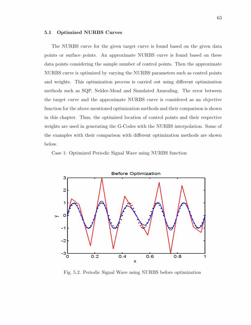
5.1 Optimized NURBS Curves
The NURBS curve for the given target curve is found based on the given data
points or surface points. An approximate NURBS curve is found based on these
data points considering the sample number of control points. Then the approximate
NURBS curve is optimized by varying the NURBS parameters such as control points
and weights. This optimization process is carried out using different optimization
methods such as SQP, Nelder-Mead and Simulated Annealing. The error between
the target curve and the approximate NURBS curve is considered as an objective
function for the above mentioned optimization methods and their comparison is shown
in this chapter. Thus, the optimized location of control points and their respective
weights are used in generating the G-Codes with the NURBS interpolation. Some of
the examples with their comparison with different optimization methods are shown
below.
Case 1: Optimized Periodic Signal Wave using NURBS function
Fig. 5.2. Periodic Signal Wave using NURBS before optimization
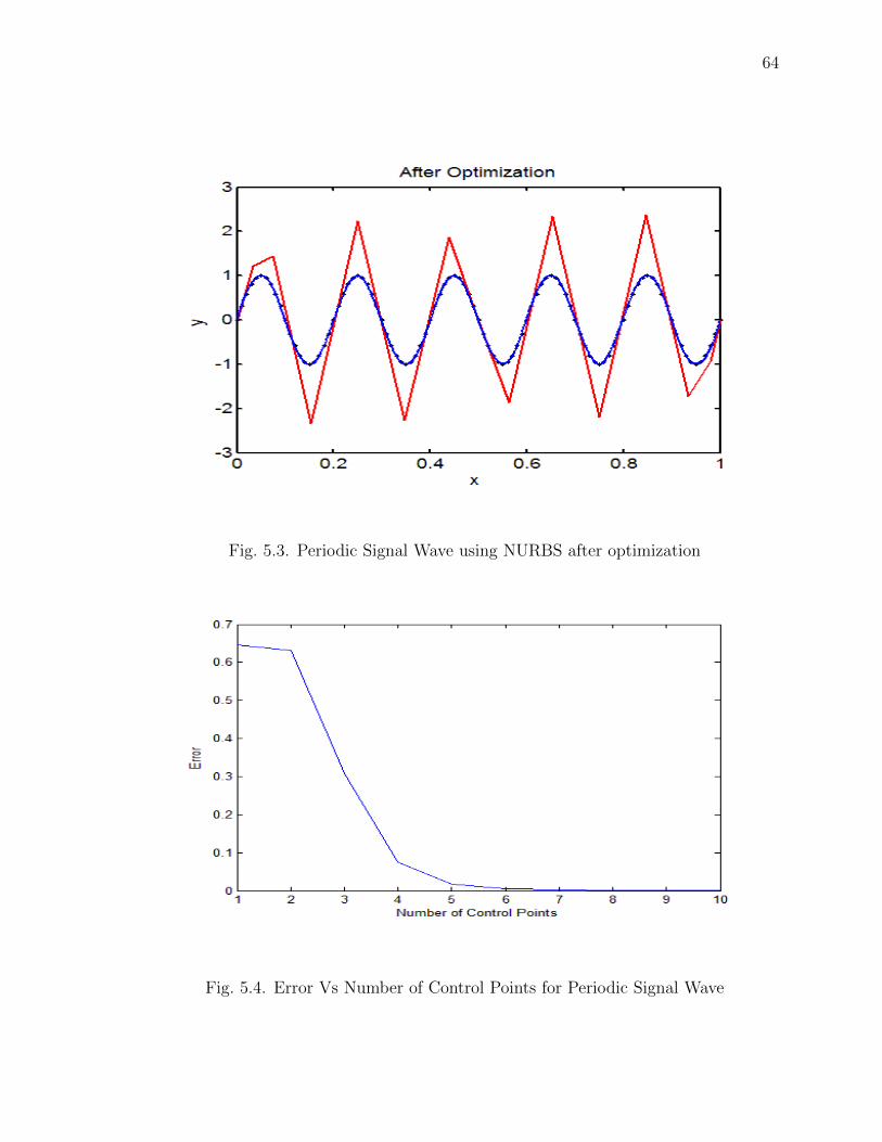
64
Fig. 5.3. Periodic Signal Wave using NURBS after optimization
Fig. 5.4. Error Vs Number of Control Points for Periodic Signal Wave

65
Fig. 5.5. Table with optimization results for Periodic Signal Wave using NURBS
Case 2: Optimized Star Shape using the NURBS Function
Fig. 5.6. Star Shape curve using NURBS before optimization

66
Fig. 5.7. Star Shape curve using NURBS after optimization
Fig. 5.8. Error Vs Number of Control Points for Star Shape curve

67
Fig. 5.9. Table with optimization results for Star Shape curve using NURBS
Case 3: Optimized Trident Curve using NURBS Function
Fig. 5.10. Trident Curve using NURBS before optimization

68
Fig. 5.11. Trident Curve using NURBS after optimization
Fig. 5.12. Error Vs Number of Control Points for Trident Curve

69
Fig. 5.13. Table with optimization results for Trident Curve using NURBS
The case studies shown above for different geometric entities significantly show
how the NURBS function can be used to represent the given target curve with the
best curve fit. It provides the flexibility to modify the shape of the entity as desired
by the developer with the change of NURBS parameters to appropriate values. In
this approach we have optimized the NURBS parameter as required to meet the
requirements of representing the target curve with the NURBS curve function with
minimum error between them. The optimization methods used in achieving this are
tabulated for each case study as shown above. If we observe that in the above case
studies the SQP method of optimization has better results than the other optimization
methods with less function calls and iterations.
5.2 NURBS Curve Representation for Pinion Gear
RACK AND PINION GEARS
A rack and pinion is a pair of gears that convert rotational motion to linear
motion. The circular pinion engages teeth on a flat bar the rack. Rotational motion
applied to the pinion by the steering wheel will cause the rack to move to one side
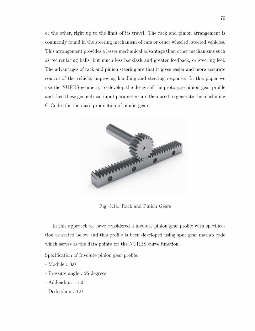
70
or the other, right up to the limit of its travel. The rack and pinion arrangement is
commonly found in the steering mechanism of cars or other wheeled, steered vehicles.
This arrangement provides a lesser mechanical advantage than other mechanisms such
as recirculating balls, but much less backlash and greater feedback, or steering feel.
The advantages of rack and pinion steering are that it gives easier and more accurate
control of the vehicle, improving handling and steering response. In this paper we
use the NURBS geometry to develop the design of the prototype pinion gear profile
and then these geometrical input parameters are then used to generate the machining
G-Codes for the mass production of pinion gears.
Fig. 5.14. Rack and Pinion Gears
In this approach we have considered a involute pinion gear profile with specifica-
tion as stated below and this profile is been developed using spur gear matlab code
which serves as the data points for the NURBS curve function.
Specification of Involute pinion gear profile:
- Module : 3.0
- Pressure angle : 25 degrees
- Addendum : 1.0
- Dedendum : 1.0

71
- Number of teeth : 10
- Pitch Circle Diameter : 30mm (Module x Number of teeth)
- Base Circle Diameter : 27.1892mm (PCD x cos(Pressure Angle))
- Tip Circle Diameter : 36mm
Based on the above specification of the involute pinion gear profile the data points
required for the NURBS curve function are extracted using the spur gear matlab
code and the figure(a) below shows the profile of complete involute pinion gear. In
this case we have considered one side of a single involute gear teeth as the target
curve because the other side of the teeth is a mirror image of the former at defined
datum plane and this is being shown in the figure (b). Now, this target curve serves
as the data points for the NURBS curve function then the approximate NURBS
curve is generated with minimum number of control points and then it is optimized
using different optimization methods to reduce the error between the target curve
and the approximate curve to as minimum as possible. Thus, these optimal NURBS
parameters with minimum error are used in generating the G-Codes using the NURBS
interpolation.
Fig. 5.15. (a) Complete Involute Pinion Gear Profile
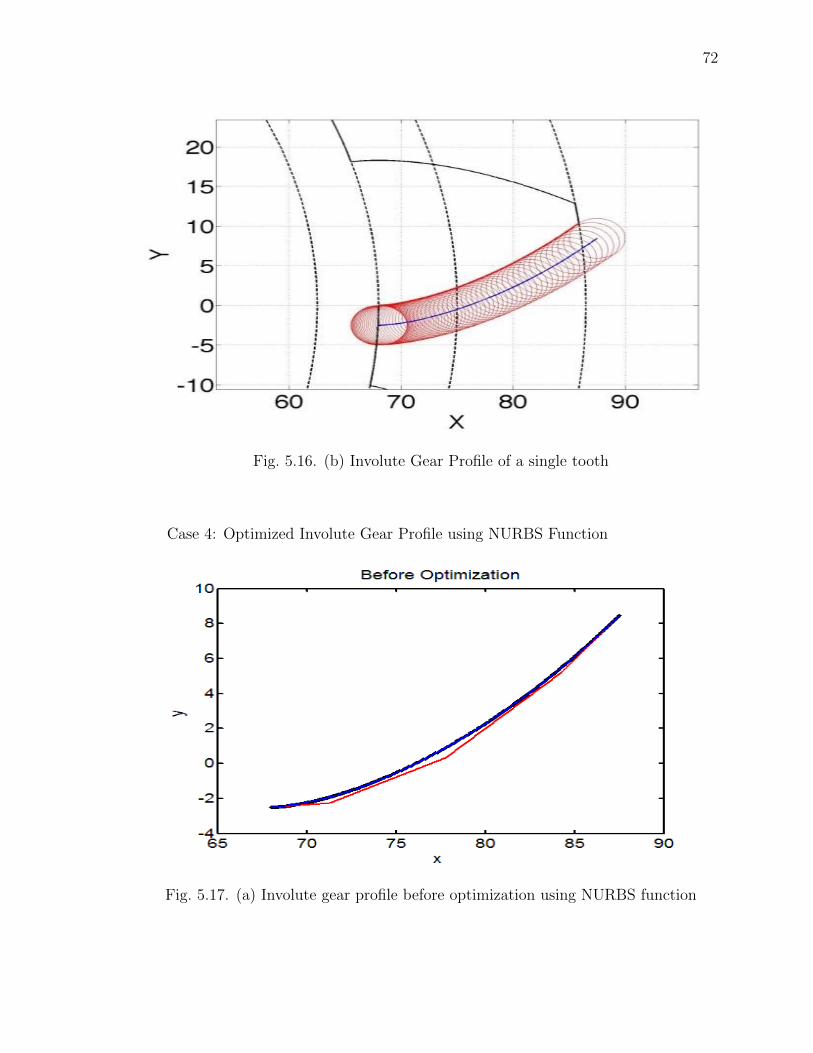
72
Fig. 5.16. (b) Involute Gear Profile of a single tooth
Case 4: Optimized Involute Gear Profile using NURBS Function
Fig. 5.17. (a) Involute gear profile before optimization using NURBS function
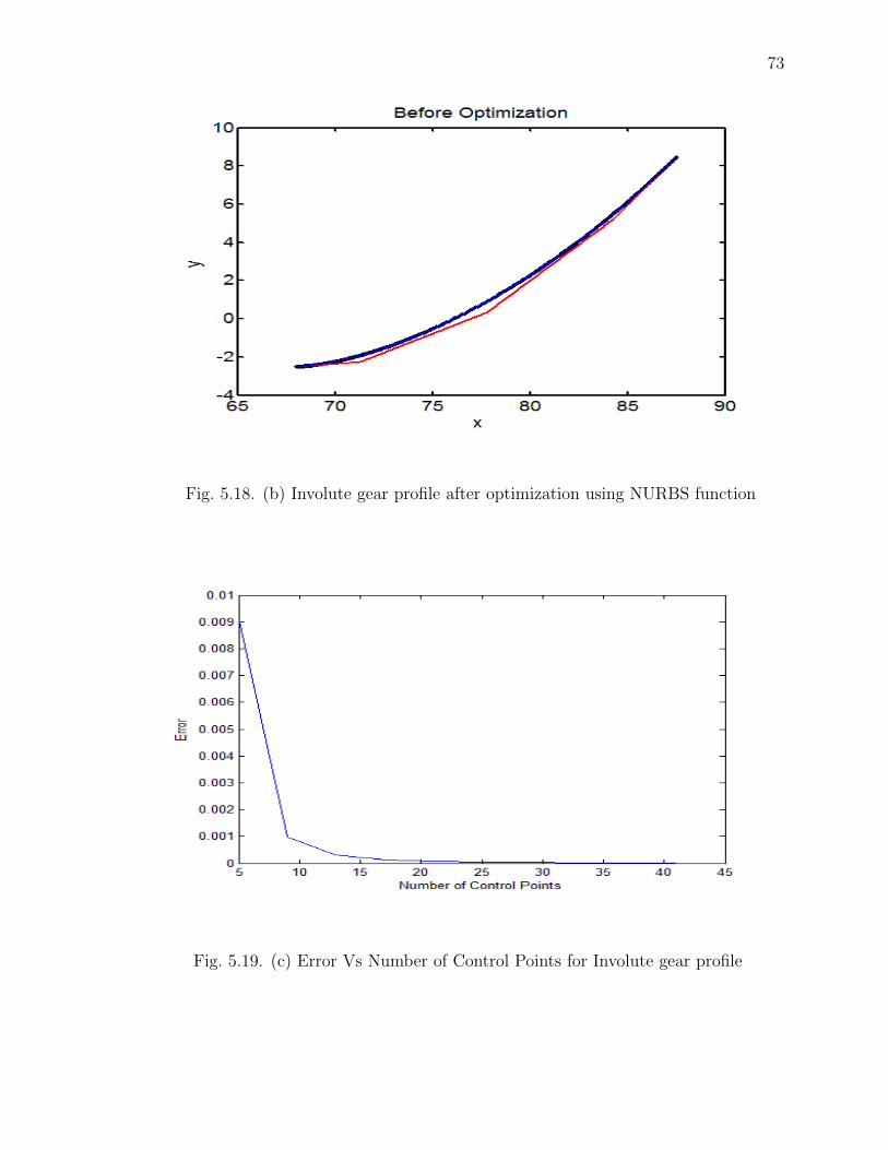
73
Fig. 5.18. (b) Involute gear profile after optimization using NURBS function
Fig. 5.19. (c) Error Vs Number of Control Points for Involute gear profile

74
Fig. 5.20. (d) Table with optimization results for Involute Gear Profileusing NURBS
Above case study shows how the involute gear profile is being represented by
NURBS curve using NURBS function. The figure (c) shows the nature of the control
points with relation to error between the target curve and the approximate NURBS
curve. An approximate curve is described that better represents the target curve
with the minimum number of control points and it has been shown in the figure
(a). This approximate curve is then optimized by varying the NURBS parameters to
the optimal values at which the error between the target curve and the approximate
NURBS curve is minimum. The figure (b) shows the optimized curve with optimal
NURBS parameters such as optimal location of control points and their respective
weighs. This optimization process is performed using different optimization methods
and their results are tabulated in figure (d). The detailed list of NURBS parameters
for the required involute gear profile before optimization and after optimization is
tabulated in figure 5.21.
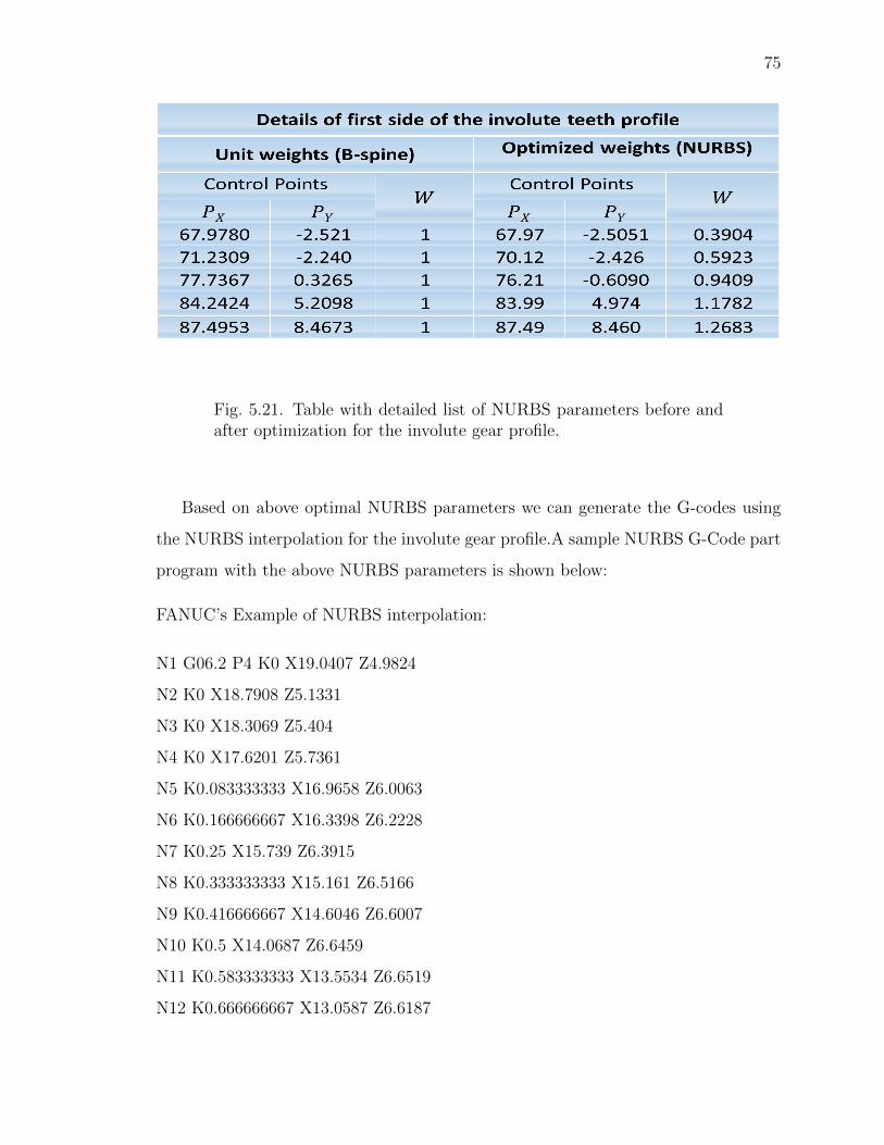
75
Fig. 5.21. Table with detailed list of NURBS parameters before andafter optimization for the involute gear profile.
Based on above optimal NURBS parameters we can generate the G-codes using
the NURBS interpolation for the involute gear profile.A sample NURBS G-Code part
program with the above NURBS parameters is shown below:
FANUC’s Example of NURBS interpolation:
N1 G06.2 P4 K0 X19.0407 Z4.9824
N2 K0 X18.7908 Z5.1331
N3 K0 X18.3069 Z5.404
N4 K0 X17.6201 Z5.7361
N5 K0.083333333 X16.9658 Z6.0063
N6 K0.166666667 X16.3398 Z6.2228
N7 K0.25 X15.739 Z6.3915
N8 K0.333333333 X15.161 Z6.5166
N9 K0.416666667 X14.6046 Z6.6007
N10 K0.5 X14.0687 Z6.6459
N11 K0.583333333 X13.5534 Z6.6519
N12 K0.666666667 X13.0587 Z6.6187
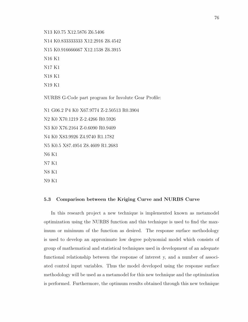
76
N13 K0.75 X12.5876 Z6.5406
N14 K0.833333333 X12.2916 Z6.4542
N15 K0.916666667 X12.1538 Z6.3915
N16 K1
N17 K1
N18 K1
N19 K1
NURBS G-Code part program for Involute Gear Profile:
N1 G06.2 P4 K0 X67.9774 Z-2.50513 R0.3904
N2 K0 X70.1219 Z-2.4266 R0.5926
N3 K0 X76.2164 Z-0.6090 R0.9409
N4 K0 X83.9926 Z4.9740 R1.1782
N5 K0.5 X87.4954 Z8.4609 R1.2683
N6 K1
N7 K1
N8 K1
N9 K1
5.3 Comparison between the Kriging Curve and NURBS Curve
In this research project a new technique is implemented known as metamodel
optimization using the NURBS function and this technique is used to find the max-
imum or minimum of the function as desired. The response surface methodology
is used to develop an approximate low degree polynomial model which consists of
group of mathematical and statistical techniques used in development of an adequate
functional relationship between the response of interest y, and a number of associ-
ated control input variables. Thus the model developed using the response surface
methodology will be used as a metamodel for this new technique and the optimization
is performed. Furthermore, the optimum results obtained through this new technique

77
are compared with the kriging (DACE function) which is commercially available tech-
nique. Some of the examples are shown below with their comparison.
Case 1: 1-Dimensional Comparison between Kriging and NURBS for a open box
function
Fig. 5.22. Comparison between Kriging and NURBS
Fig. 5.23. Comparison between Kriging and NURBS
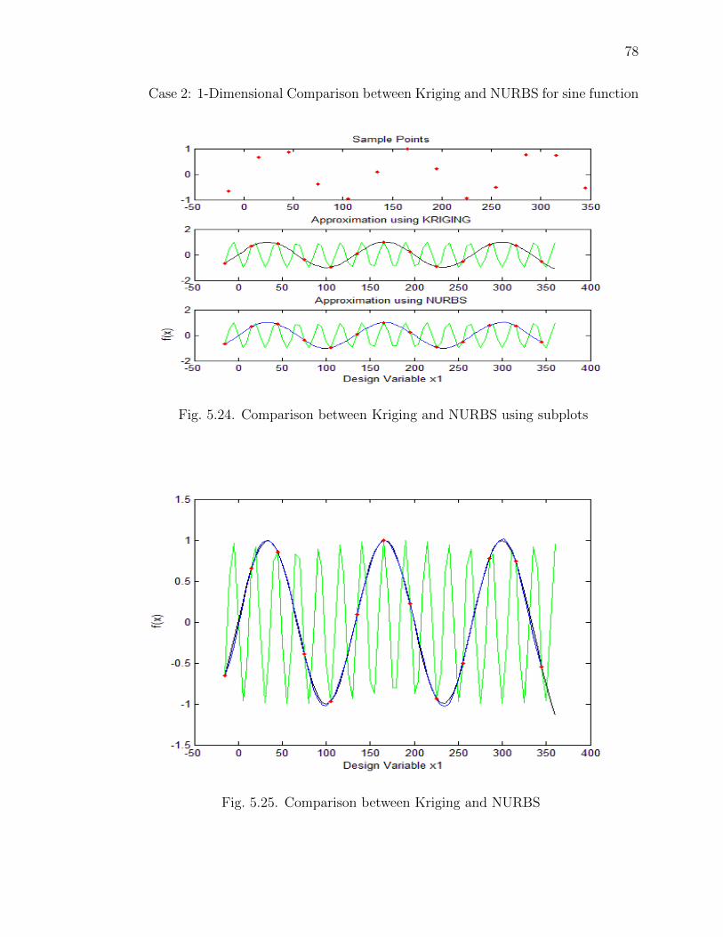
78
Case 2: 1-Dimensional Comparison between Kriging and NURBS for sine function
Fig. 5.24. Comparison between Kriging and NURBS using subplots
Fig. 5.25. Comparison between Kriging and NURBS
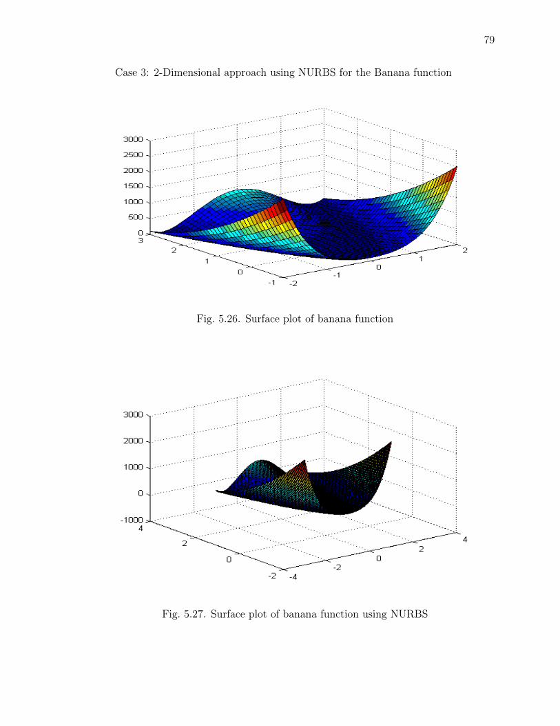
79
Case 3: 2-Dimensional approach using NURBS for the Banana function
Fig. 5.26. Surface plot of banana function
Fig. 5.27. Surface plot of banana function using NURBS

80
Fig. 5.28. Contour plot of banana function
Fig. 5.29. Contour plot of banana function using NURBS
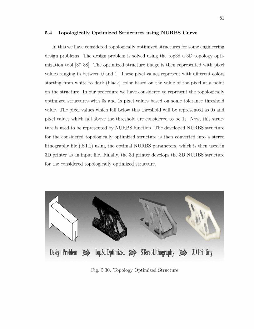
81
5.4 Topologically Optimized Structures using NURBS Curve
In this we have considered topologically optimized structures for some engineering
design problems. The design problem is solved using the top3d a 3D topology opti-
mization tool [37, 38]. The optimized structure image is then represented with pixel
values ranging in between 0 and 1. These pixel values represent with different colors
starting from white to dark (black) color based on the value of the pixel at a point
on the structure. In our procedure we have considered to represent the topologically
optimized structures with 0s and 1s pixel values based on some tolerance threshold
value. The pixel values which fall below this threshold will be represented as 0s and
pixel values which fall above the threshold are considered to be 1s. Now, this struc-
ture is used to be represented by NURBS function. The developed NURBS structure
for the considered topologically optimized structure is then converted into a stereo
lithography file (.STL) using the optimal NURBS parameters, which is then used in
3D printer as an input file. Finally, the 3d printer develops the 3D NURBS structure
for the considered topologically optimized structure.
Fig. 5.30. Topology Optimized Structure

82
Fig. 5.31. (a) Topology optimized structure and (b) Topology opti-mized structure with pixel values 0s and 1s
The figures above show the pixel representation of the considered topologically
optimized structure. The figure (a) represents structure before conversion and figure
(b) represents structure after conversion of the pixel values based on the threshold
value to represent the above structure using the NURBS function.
Boundary Representation and Generation of NURBS curves:
Once the conversion of the pixel values based on the threshold is done of the con-
sidered structure, then we find all the boundaries of the structure based on the pixel
locations on the structure for both closed and open loop. These boundary represen-
tation points serves as a data or surface points for the NURBS function. Then these
data points are used in representation of the structure using NURBS for each bound-
ary of the structure. An example is shown below for both boundary representation
and NURBS Structure generation using NURBS function.
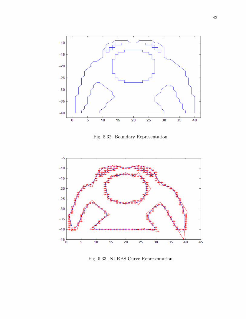
83
Fig. 5.32. Boundary Representation
Fig. 5.33. NURBS Curve Representation

84
3D structure development using 3ds max software with NURBS optimal parameter:
The 3ds max software is used in developing the 3D structure using the NURBS
optimal parameters. In this software we consider the NURBS optimal control points
and their respective weights in developing the topologically optimized structure. After
development of the structure using the NURBS parameter it is then imported into
Pro-Engineering Software which then converts the 3D structure developed in 3ds max
into stereo lithography file (.stl) which is our required file format which is using in
the 3D Printer. An example is shown below with the developed structure using 3ds
software and then importing in Pro-Engineering software for correct file format. Thus,
the file created in Pro-E is used as an input file in 3d printer and a sample structure
is shown in the figure below.
Fig. 5.34. Topological optimized structure developed using 3ds soft-ware with NURBS optimal parameters.
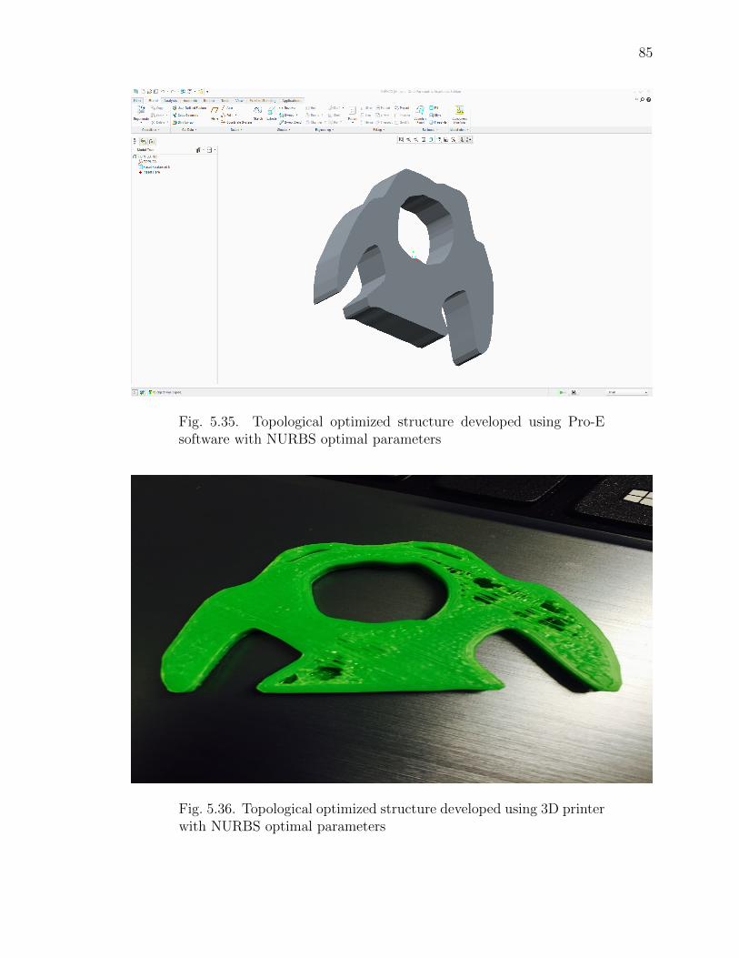
85
Fig. 5.35. Topological optimized structure developed using Pro-Esoftware with NURBS optimal parameters
Fig. 5.36. Topological optimized structure developed using 3D printerwith NURBS optimal parameters
86
6. CONCLUSIONS
This chapter presents an overview and general conclusions related to the work devel-
oped in this dissertation and recommendations for future work.
6.1 Summary
6.1.1 Optimized NURBS Curves
1. Successful implementation of developed NURBS function on different geometric
entities such as Periodic Signal wave, Trident Curve and Star shape, Pinion Gear
Profile was demonstrated.
2. The approximate NURBS curve is optimized using different optimization meth-
ods and their comparison are shown. It was observed that the SQP optimization
methods is the most efficient way to find the best location of control points and
their corresponding weights to represent the target curve with the results and
observations shown in chapter 5.
3. Comparison between the developed NURBS function and the kriging function
(DACE function) is demonstrated with several examples.
4. Examples: Representation of Periodic signal wave, Trident Curve and star
shape, Pinion Gear Profile using the NURBS function was demonstrated with all
the optimization results and their comparison. Also, shows the graph between
the number of control points and the error function which results in effective
selection of number of control points.
87
5. Finally, these optimized data of location of control points and their correspond-
ing weights have been used in generating the G-Codes using the NURBS Inter-
polation for the pinion gear.
6.1.2 Topologically Optimized Structures using NURBS Curve
1. In this research approach we have considered a topologically optimized struc-
ture and then we have reconstructed the structure with desired pixel values.
This incorporates in defining all the boundaries of the given structure. These
boundaries are then used as the data points for the NURBS function and then
a structure is developed using the NURBS function with optimal parameters.
2. These optimal parameters are used in 3ds max software which incorporates the
use of NURBS functionality which is used in developing a 3D structure and this
is been successfully demonstrated in chapter 5.
3. This 3D structure from 3ds max software is then imported into Pro-Engineer
software to convert into required stereo lithography file and it is also been shown
in chapter 5.
4. Thus, this stereo lithography file is been used as an input file for 3D Printer
machine and finally, 3D product of the given topologically optimized structure
with NURBS function is developed and well demonstrated.
6.2 Original Contributions
The requirements for advanced functions to support high-speed machining and
high-accuracy machining which are generally used is growing. In particular, when
conventional CNC systems where free curve is defined by sequential small line seg-
ments or arcs are used for machining free-form surfaces, the tool moves in a discon-
tinuous manner and this makes the quality of the machined surface poor. The size

88
of the program will be large as it involves a lot of block programs as required. To
overcome this problem NURBS interpolation was developed.
In NURBS interpolation, NURBS curve parameters such as the control points,
weights and knot vector are directly fed as an input to the CNC system instead of
the small line segment data that are defined by G01 command. As the CNC system
generates interpolation points based on NURBS curve parameters, the programmed
federate and the tolerance, it makes it possible to perform high-speed machining and
high-accuracy machining.
The conclusion from this research is that the pinion gear profile was developed
using the NURBS curves and the resultant approximate curves are optimized us-
ing NelderMead, SQP and Simulated annealing methods. We found that the SQP
method for optimization is the most efficient way to find the best location of con-
trol points and their corresponding weights to represent the target curve with the
results and observations shown. The comparison between the NURBS function and
kriging function (DACE function) is served as a validation of the developed method-
ology approach. Finally, these optimized data of location of control points and their
corresponding weights have been used in generating the G-Codes using the NURBS
Interpolation for the pinion gear. Also, the use of NURBS function in representing
the topologically optimized structures and 3D printing it.
6.3 Future Recommendations
1. The NURBS interpolation G-Codes can be used in 3D printer instead of using
the linear interpolation and circular interpolation. This would enhance the
performance and the surface finish of the product desired.
2. This approach of metalmodel using the NURBS function can used in Simulink
Model especially in library blocks such as lookup tables where cubic interpola-
tion is desired. This will help in selection of correct response for the given input
parameters.

89
3. There is a high possibility that we can use this developed NURBS function for
optimizing higher derivatives such as tool path fluctuation, feed rate and etc.

REFERENCES

90
REFERENCES
[1] J. Liu, B. C. M. Liu, D. Xu, and Y. Li, An Optimization of NURBS interpola-tion algorithm. IEEE 10th International Conference on Industrial InformaticsIndustrial Informatics (INDIN), 2012 10th IEEE International Conference on.:316-319 Jul, 2012.
[2] Y.-L. Lai, Tool-path generation of planar curves, 2nd ed. Robotics andComputer-Integrated Manufacturing 26, 2010.
[3] Z. Jing, F. Shaowei, and C. Hanguo, Optimized NURBS Curve and SurfaceFitting using simulated Annealing, 3rd ed. Second international symposium onComputational Intelligence and Design, 2009.
[4] H. Ameddah and M. Assas, NURBS Interpolation Strategies of Complex Surfacesin High Speed Machining. International Journal of CAD/CAM Vol. 11 No. 1pp. 00-00, 2011.
[5] J. Jahanpour and M. Alizadeh, A novel acc-jerk-limited NURBS interpolationenhanced with an optimized S-shaped quintic feedrate scheduling scheme. Inter-national Journal of Advanced Manufacturing Technology. Apr2015, Vol. 77 Issue9-12, p1889-1905. 17p. 2 Diagrams, 5 Charts, 10 Graphs.
[6] Y. Zhang, C. Lu, Y. Lin, and J. Hu, Improvement of Quantum-Behaved Parti-cle Swarm Optimization Algorithm and Its Application to Ship Hull WaterlinesApproximation Based on Non-Uniform Rational B-Spline. Journal of Ship Pro-duction and Design. Nov2017, Vol. 33 Issue 4, p357-365. 9p.
[7] P. Kang and S.-K. Youn, Isogeometric topology optimization of shell structuresusing trimmed NURBS surfaces. Finite Elements in Analysis and Design.Nov2016, Vol. 120, p18-40. 23p.
[8] D. HU and J. Guo, Tool path optimization algorithm of spatial cam flank millingbased on NURBS surface. Journal of the Brazilian Society of Mechanical Sci-ences and Engineering; April 2018, Vol. 40 Issue: 4 p1-8, 8p.
[9] D. Saini, S. Kumar, and T. R. Gulati, NURBS-based geometric inverse recon-struction of free-form shapes. Journal of King Saud University: Computer andInformation Sciences, Vol 29, Iss 1, Pp 116-133 (2017).
[10] T. R. Gulati, D. Saini, and S. Kumar, Reconstruction of free-form space curvesusing NURBS-snakes and a quadratic programming approach. Computer AidedGeometric Design. Feb2015, Vol. 33, p30-45. 16p.
[11] Y.-J. Yang, W. Zeng, and T.-Q. Song, Optimizing conformality of NURBS sur-faces by general bilinear transformations. Computer Aided Geometric Design.Feb2015, Vol. 33, p30-45. 16p.
91
[12] L. Huang, J. Zhen, and X. Zhu, Approach for Approximating ArbitraryCurves by NURBS. School of Mechanical Engineering and Automa-tion, Beijing University of Aeronautics and Astronautics, Beijing, 100083,http://www.linghuang.org/research/paper/curve.htm.
[13] Y. L. Lai, J. H. Chen, and J. P.Hung, Development of Machinable Ellipses byNURBS Curves. International Journal of Aerospace and Mechanical Engineering2:1, 2008.
[14] A. S. Wen, S. M. H. Shamsuddin, and Y. Samian, Optimized NURBS Ship HullFitting using Simulated Annealing. Imaging and Visualization (CGIV,06): Pro-ceeding of the International Conference on Computer Graphics.
[15] A. Hashemian and S. F. Hosseini, An integrated fitting and fairing approach forobject reconstruction using smooth NURBS curves and surfaces. Computers andMathematics with Applications. Oct2018, Vol. 76 Issue 7, p1555-1575. 21p.
[16] H. Zhou, J. Wu, X. Tang, and J. Chen, Research and implementation of NURBSinterpolator with continuous feedrate for high-speed machining. InternationalJournal of Production Research. Nov2012, Vol. 50 Issue 22, p6457-6468. 12p. 2Color Photographs, 2 Black and White Photographs, 7 Diagrams, 2 Charts, 4Graphs.
[17] M. Sekar and Y. S. Han, Design and Implementation of High-Performance Real-Time Free-Form NURBS Interpolator in Micro CNC Machine Tool. MechanicsBased Design of Structures and Machines. Jul-Sep2014, Vol. 42 Issue 3, p296-311.16p.
[18] M. Liu, Y. Huang, J. Guo, X. Shao, and G. Zhang, Development and implementa-tion of a NURBS interpolator with smooth feedrate scheduling for CNC machinetools. International Journal of Machine Tools and Manufacture. Dec2014, Vol.87, p1-15. 15p.
[19] S. Liang, Wansheng, and X. Xi, Design of a real-time NURBS interpolator withconstant segment length for milling EDM. International Journal of AdvancedManufacturing Technology. Jul2013, Vol. 67 Issue 1-4, p427-440. 14p. 1 ColorPhotograph, 9 Diagrams, 1 Chart, 5 Graphs.
[20] J.-B. Wang and H.-T. Yau, Universal real-time NURBS interpolator on a PC-based controller. International Journal of Advanced Manufacturing Technology.Mar2014, Vol. 71 Issue 1-4, p497-507. 11p. 1 Color Photograph, 7 Diagrams, 2Charts, 6 Graphs.
[21] J. Lepine, F. Guibault, M.-G. Vallet, and J.-Y. Trepanier, Optimization of acurve Approximation Based on NURBS interpolation. International Conferenceon Curve and Surface Design: Saint-Malo, 1999.
[22] L. Piegl and W. Tiller, The NURBS Book. New York : Springer, c1995.
[23] I. Zeid, Mastering CAD/CAM. New Delhi : McGraw-Hill Education (India),2007, 2005.
[24] L. Piegl, On NURBS: A Survey. IEEE Computer Graphics and Applica-tions IEEE Comput. Grap. Appl. Computer Graphics and Applications, IEEE.11(1):55-71 Jan, 1991.
92
[25] S.-H. Suh, S.-K. Kang, D.-H. Chung, and I. Stroud, Theory and Design of CNCSystems. Springer Series in Advanced Manufacturing, London : Springer-Verlag,2008.
[26] Y. Zhao, X.-W. Shi, and L. Xu, Modeling with NURBS Surfaces used for thecalculation of RCS. Progress In Electromagnetics Research, PIER 78, 4959,2008.
[27] S.-S. Yeh and S.-C. Su, Design of NURBS Curve Fitting Process on CNC Ma-chines. Proceedings of the 2007 American Control Conference, 2007.
[28] H. Liang and X. Li, A 5-axis Milling System Based on a New G code for NURBSSurface. 2009 IEEE International Conference on Intelligent Computing andIntelligent Systems Intelligent Computing and Intelligent Systems, 2009. ICIS2009. IEEE International Conference on. 2:600-606 Nov, 2009.
[29] Fanuc Series 15i by 150i Model A. Operators Manual by FANUC.
[30] C. Liangji and F. Xianzhang, Method of NURBS Interpolation with ACC/DECControlling in 5-axis CNC System. INC2010: 6th International Conferenceon Networked Computing Networked Computing (INC), 2010 6th InternationalConference on. :1-4 May, 2010.
[31] H. Qingyao, L. Anwen, Y. Ying, and Y. Shuhui, NC machining for steam tur-bine blade based on NURBS curve ACC/DEC interpolation algorithm. 2011International Conference on Consumer Electronics, Communications and Net-works (CECNet) Consumer Electronics, Communications and Networks (CEC-Net), 2011 International Conference on. :495-498 Apr, 2011.
[32] NURBS Modeling. Version 6, Alias Systems.
[33] FANUC Series 31i Model A. Operators Manual by FANUC.
[34] X. Jiazhong, Z. Lei, and Q. Ming, Research on Electronic Cam Based onNurbs Interpolation Algorithm. 2009 9th International Conference on Elec-tronic Measurement and Instruments Electronic Measurement and Instruments,2009. ICEMI ’09. 9th International Conference on. :4-669-4-674 Aug, 2009.
[35] F. Gao and L. Han, Implementing the Nelder-Mead simplex algorithm with adap-tive parameters. Springer Science + Business Media, LLC, 2010.
[36] J. C.Lagarias, J. A. Reeds, M. H. Wright, and P. E. Wright, Convergence proper-ties of the Nelder-Mead simplex algorithm in low dimensions. SIAM J. Optim.9, 112147, 1998.
[37] O. Sigmund, A 99 line topology optimization code written in Matlab. StructMultidisc Optim 21, 120127.
[38] K. Liu and A. Tovar, An efficient 3D topology optimization code written in Mat-lab. Structural and multidisciplinary Optimization, United States, North Amer-ica: Springer, 2015.
93
[39] Z. Tang, W. Xia, F. Li, Z. Zhou, and J. Zhao, Application of response surfacemethodology in the optimization of burnishing parameters for surface integrity.2010 International Conference on Mechanic Automation and Control Engineer-ing Mechanic Automation and Control Engineering (MACE), 2010 InternationalConference on. :3887-3890 Jun, 2010.
[40] M. Demirel1, B. Kayan2, Demirel, and Kayan, Application of response sur-face methodology and central composite design for the optimization of textile dyedegradation by wet air oxidation. International Journal of Industrial Chemistry2012, 3:24, 2012.
[41] S. N. Lophaven, H. B. Nielsen, and J. Sndergaard, DACE A MatLab KrigingToolbox. Information and Mathematical Modeling(IMM), Version 2.0, August1, 2002.

APPENDICES

94
A. KRIGING FUNCTION
The kriging approximate model is constructed based on the experimental data and
this is used as a surrogate model for the original experiment model [39–41]. This
surrogate model has a collection of inputs and their responses based on the original
experiment model. These inputs and their responses are usually considered to be
high dimensional. The purpose of using this kriging model is to find the response of
the original model at unknown or untried input parameter values. The result of the
kriging is the expected value and variance computed for each and every point within
the region. This is practically done on a fine enough grid.
Suppose we observe some variable Z along 1-dim space (X). There are 5 mea-
surements made. We might ask ourselves, knowing the probabilistic behavior of the
random field being observed, what are possible trajectories (realizations) of the ran-
dom field, that agree with the data? This is answered by conditional simulation
Fig. A.1. Representation of curves using Kriging
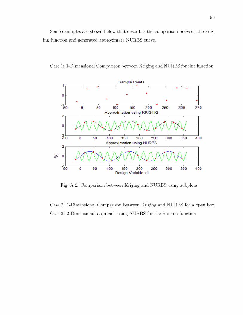
95
Some examples are shown below that describes the comparison between the krig-
ing function and generated approximate NURBS curve.
Case 1: 1-Dimensional Comparison between Kriging and NURBS for sine function.
Fig. A.2. Comparison between Kriging and NURBS using subplots
Case 2: 1-Dimensional Comparison between Kriging and NURBS for a open box
Case 3: 2-Dimensional approach using NURBS for the Banana function
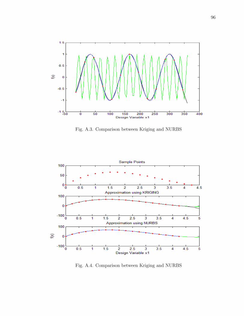
96
Fig. A.3. Comparison between Kriging and NURBS
Fig. A.4. Comparison between Kriging and NURBS
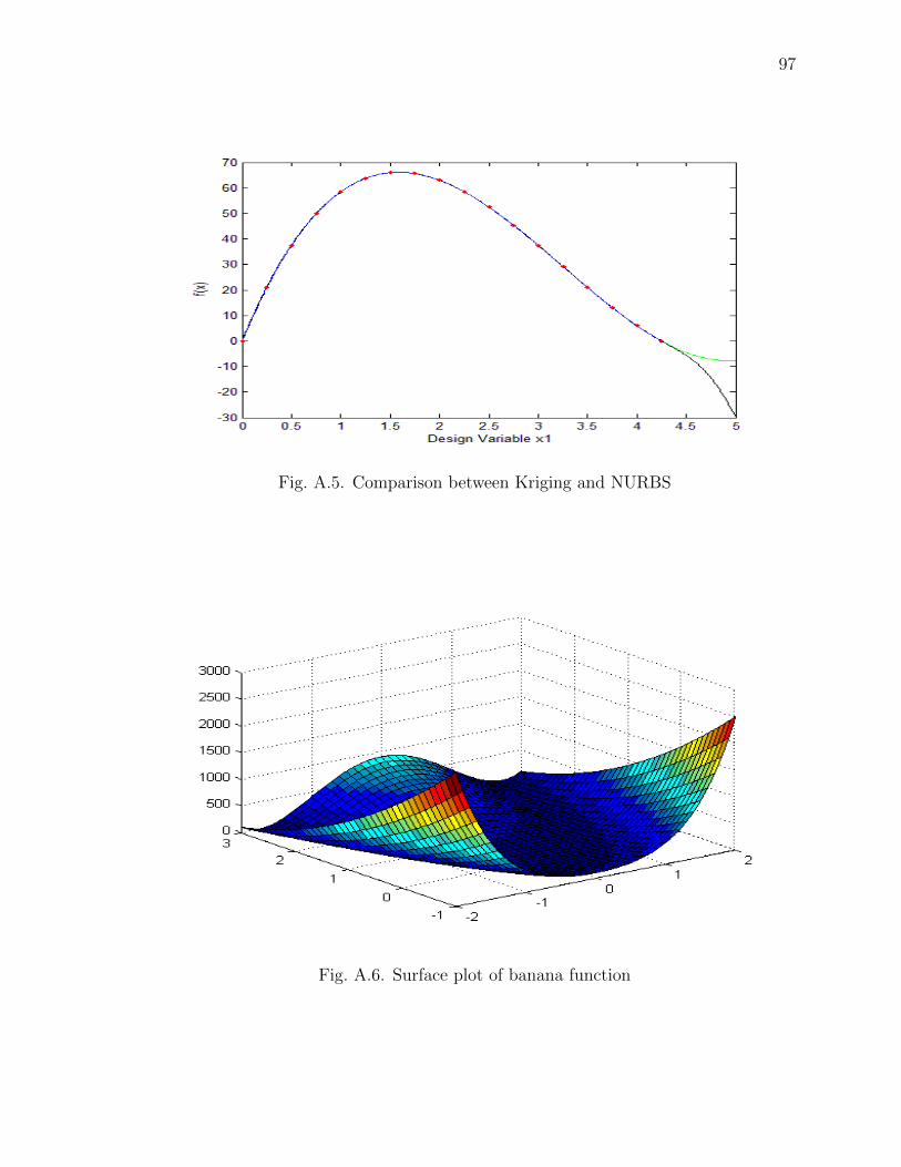
97
Fig. A.5. Comparison between Kriging and NURBS
Fig. A.6. Surface plot of banana function
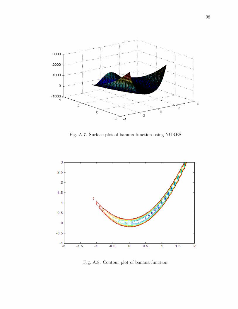
98
Fig. A.7. Surface plot of banana function using NURBS
Fig. A.8. Contour plot of banana function
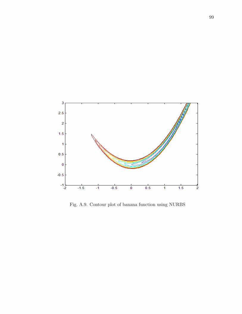
99
Fig. A.9. Contour plot of banana function using NURBS
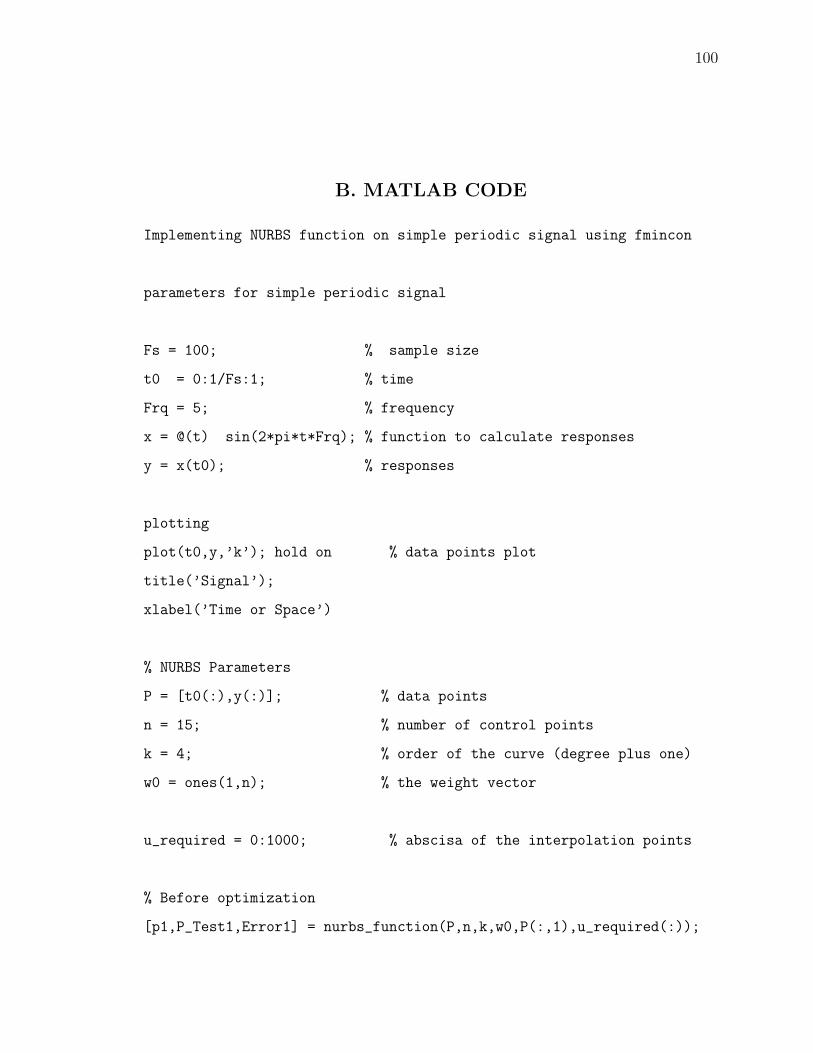
100
B. MATLAB CODE
Implementing NURBS function on simple periodic signal using fmincon
parameters for simple periodic signal
Fs = 100; % sample size
t0 = 0:1/Fs:1; % time
Frq = 5; % frequency
x = @(t) sin(2*pi*t*Frq); % function to calculate responses
y = x(t0); % responses
plotting
plot(t0,y,’k’); hold on % data points plot
title(’Signal’);
xlabel(’Time or Space’)
% NURBS Parameters
P = [t0(:),y(:)]; % data points
n = 15; % number of control points
k = 4; % order of the curve (degree plus one)
w0 = ones(1,n); % the weight vector
u_required = 0:1000; % abscisa of the interpolation points
% Before optimization
[p1,P_Test1,Error1] = nurbs_function(P,n,k,w0,P(:,1),u_required(:));
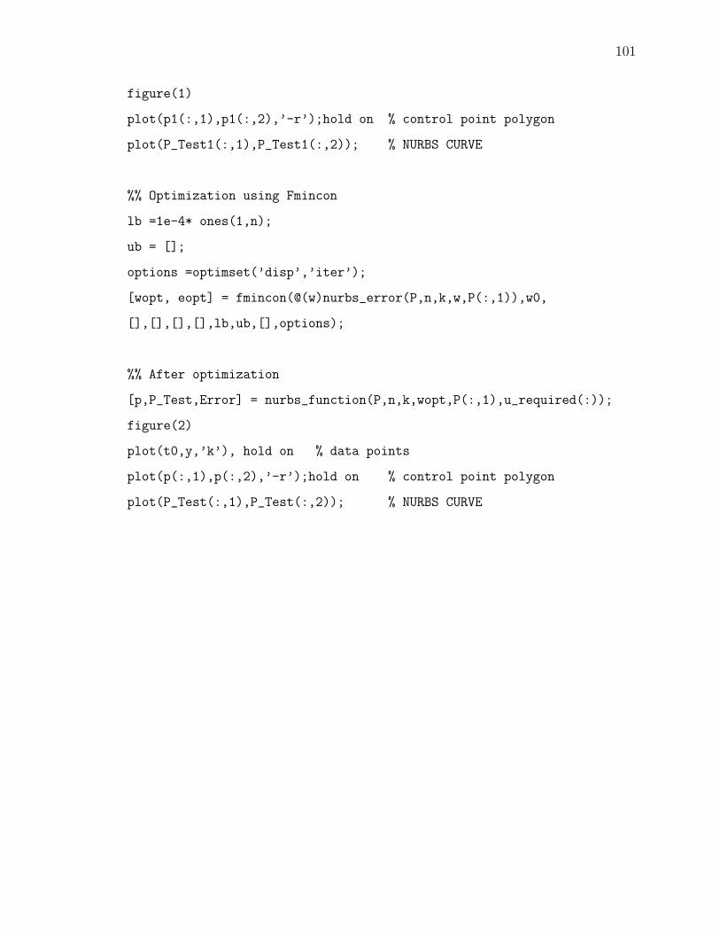
101
figure(1)
plot(p1(:,1),p1(:,2),’-r’);hold on % control point polygon
plot(P_Test1(:,1),P_Test1(:,2)); % NURBS CURVE
%% Optimization using Fmincon
lb =1e-4* ones(1,n);
ub = [];
options =optimset(’disp’,’iter’);
[wopt, eopt] = fmincon(@(w)nurbs_error(P,n,k,w,P(:,1)),w0,
[],[],[],[],lb,ub,[],options);
%% After optimization
[p,P_Test,Error] = nurbs_function(P,n,k,wopt,P(:,1),u_required(:));
figure(2)
plot(t0,y,’k’), hold on % data points
plot(p(:,1),p(:,2),’-r’);hold on % control point polygon
plot(P_Test(:,1),P_Test(:,2)); % NURBS CURVE

102
NURBS_FUNCTION.m:
function [p,P_Test1,Error] = nurbs_function(P,n,k,w,u_ini,u_required)
%%
% This function is used for generating the NURBS curve for the given
% data points that provide the deliverables as control points,
% resultant data points and error between the target curve and nurbs
% curve.
% P - Data points of the given model
% n - Number of Control Points
% k - Order of the Curve
% w - Weight vector for the selected Number of Control Points
% (initailly taken as all ones)
% u_ini - Design Variable Set
% u_required - Interpolation Points
%%
a = numel(u_ini(:,1));
b = numel(u_ini(1,:));
u_mid = zeros(a,b);
% //////*************** Parametric Variable ****************//////
for i=1:numel(u_ini(1,:))
u_mid(:,i) = ParametricVariable(u_ini(:,i));
end
u = arrangement(u_mid);
% /////************* Computing the Knot Vector *************/////
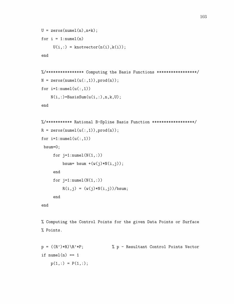
103
U = zeros(numel(n),n+k);
for i = 1:numel(n)
U(i,:) = knotvector(n(i),k(i));
end
%/**************** Computing the Basis Functions *****************/
N = zeros(numel(u(:,1)),prod(n));
for i=1:numel(u(:,1))
N(i,:)=BasisSum(u(i,:),n,k,U);
end
%/*********** Rational B-Spline Basis Function ******************/
R = zeros(numel(u(:,1)),prod(n));
for i=1:numel(u(:,1))
bsum=0;
for j=1:numel(N(1,:))
bsum= bsum +(w(j)*N(i,j));
end
for j=1:numel(N(1,:))
R(i,j) = (w(j)*N(i,j))/bsum;
end
end
% Computing the Control Points for the given Data Points or Surface
% Points.
p = ((R’)*R)\R’*P; % p - Resultant Control Points Vector
if numel(n) == 1
p(1,:) = P(1,:);

104
p(numel(p(:,1)),:) = P(numel(P(:,1)),:);
end
% for error
P_Test = nurbstest(p,u,n,k,w); % ’nurbstest’ function
% is used to find the data points for the given control points
% for plotting
P_Test1 = nurbstest(p,u_required,n,k,w);
% Error Calculation
di = 0;
dif = zeros(1, numel(P(:,1)));
for j=1:(numel(P(:,1)))
dif(j)=((P(j,1)-P_Test(j,1))^2+(P(j,2)-P_Test(j,2))^2)^(1/2);
di= di + dif(j);
end
Error = di/(numel(P)/2);
end
PARAMETRIC VARIABLE:
function u=ParametricVariable(P)
% Note
% P - Position Vector
t=0;
temp=0;
t_max=1;
u=zeros(size(P));

105
for r=2:numel(u)
z=P(r)- P(r-1);
if z<0
z=(-1)*z;
end
temp=temp+z;
end
for s=2:numel(u)
for r=2:s
x= P(r)- P(r-1);
if x<0
x=(-1)*x;
end
t=t+x;
end
u(s)=(t*(t_max/temp));
t=0;
end
end
ARRANGEMENT CODE:
function N = arrangement(P)
% P - Matrix consisting of all design variable vectors in

106
% column wise.
n = numel(P(1,:)); % n - Number of Columns
N = zeros(numel(P(:,1))^n,n); % N - All the combinations
for the given desugn Variables
for i = 1:n
c = 1; % c - Count for number of rows
l = 0; % l - Number of intervals of each design variable
for j=1:numel(P(:,i))^i
for k=1:numel(P(:,i))^(n-i)
N(c,i)= P(j-l*numel(P(:,i)),i);
c=c+1;
end
if j == (l+1)*(numel(P(:,i)))^i/(numel(P(:,i))^(i-1))
l= l+1;
end
end
end
end
KNOT VECTOR CODE:
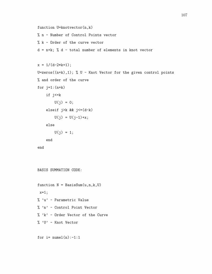
107
function U=knotvector(n,k)
% n - Number of Control Points vector
% k - Order of the curve vector
d = n+k; % d - total number of elements in knot vector
x = 1/(d-2*k+1);
U=zeros((n+k),1); % U - Knot Vector for the given control points
% and order of the curve
for j=1:(n+k)
if j<=k
U(j) = 0;
elseif j>k && j<=(d-k)
U(j) = U(j-1)+x;
else
U(j) = 1;
end
end
BASIS SUMMATION CODE:
function N = BasisSum(u,n,k,U)
x=1;
% ’u’ - Parametric Value
% ’n’ - Control Point Vector
% ’k’ - Order Vector of the Curve
% ’U’ - Knot Vector
for i= numel(n):-1:1
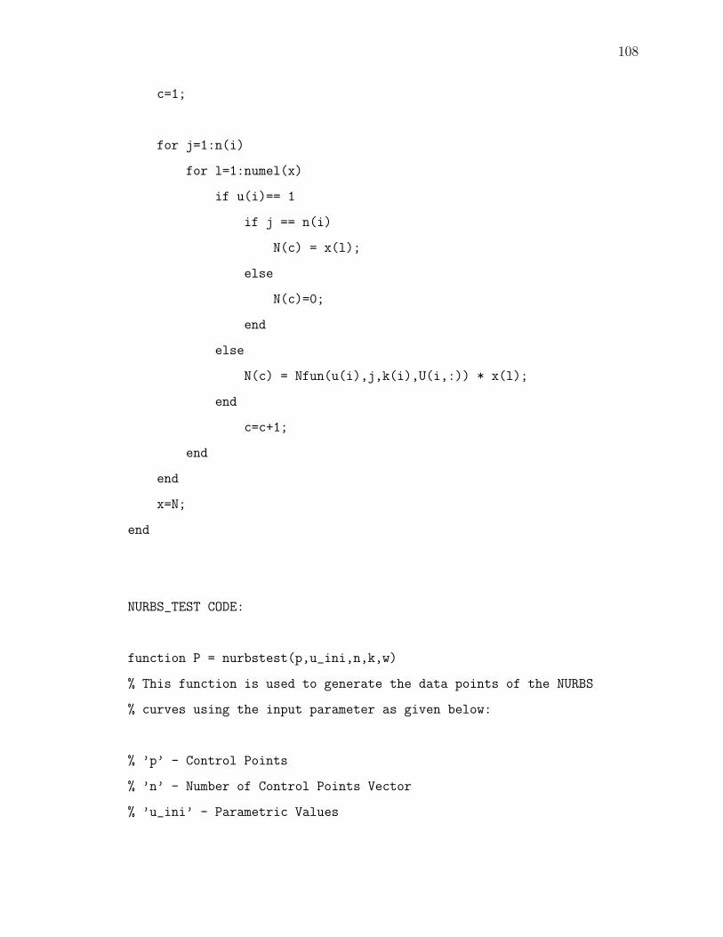
108
c=1;
for j=1:n(i)
for l=1:numel(x)
if u(i)== 1
if j == n(i)
N(c) = x(l);
else
N(c)=0;
end
else
N(c) = Nfun(u(i),j,k(i),U(i,:)) * x(l);
end
c=c+1;
end
end
x=N;
end
NURBS_TEST CODE:
function P = nurbstest(p,u_ini,n,k,w)
% This function is used to generate the data points of the NURBS
% curves using the input parameter as given below:
% ’p’ - Control Points
% ’n’ - Number of Control Points Vector
% ’u_ini’ - Parametric Values

109
% ’k’ - Order of the curve
% ’w’ - Weight vector
%************* Parametric Values **********************%
u_mid = zeros(numel(u_ini(:,1)), numel(u_ini(1,:)));
for i=1:numel(u_ini(1,:))
u_mid(:,i) = ParametricVariable(u_ini(:,i));
end
u = arrangement(u_mid);
%************* Computing the Knot Vector****************
U = zeros(numel(n),n+k);
for i = 1:numel(n)
U(i,:) = knotvector(n(i),k(i));
end
% Basis functions N and the parametric equation P
N = zeros(numel(u(:,1)),prod(n));
for i=1:numel(u(:,1))
N(i,:)=BasisSum(u(i,:),n,k,U);
end
%/*********** Rational B-Spline Basis Function ******************/
R = zeros(numel(u(:,1)),prod(n));
for i=1:numel(u(:,1))
bsum=0;
for j=1:numel(N(1,:))
bsum= bsum +(w(j)*N(i,j));
end
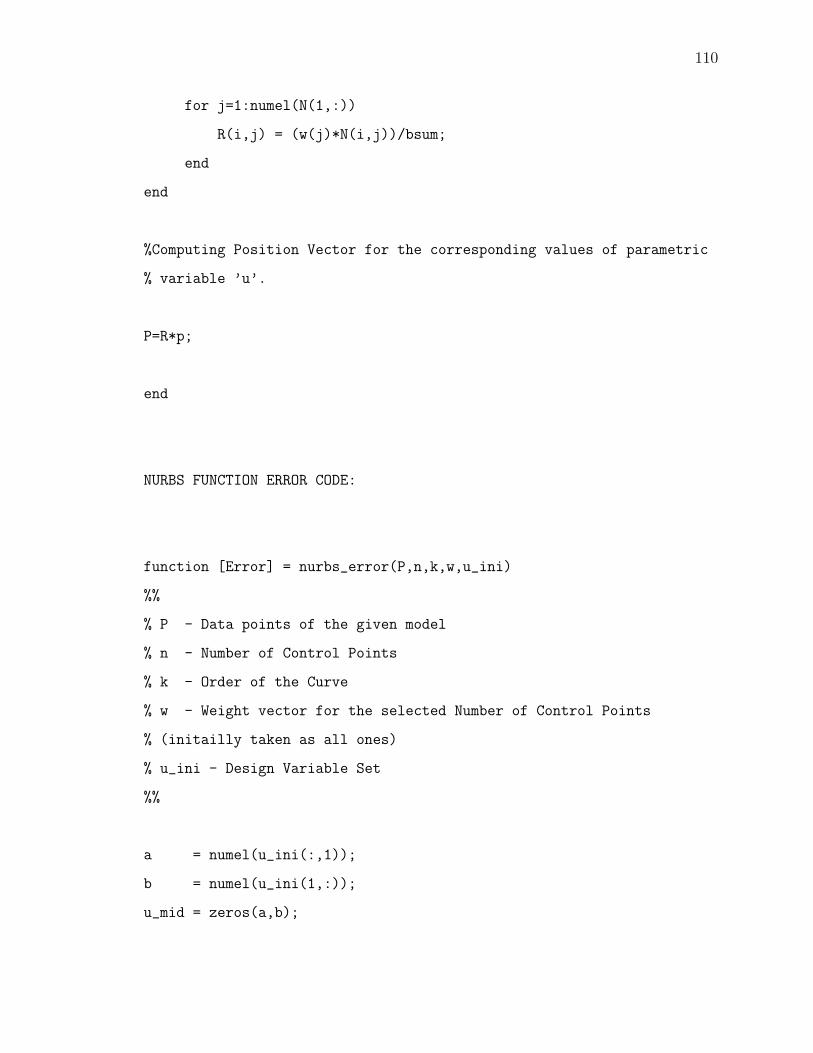
110
for j=1:numel(N(1,:))
R(i,j) = (w(j)*N(i,j))/bsum;
end
end
%Computing Position Vector for the corresponding values of parametric
% variable ’u’.
P=R*p;
end
NURBS FUNCTION ERROR CODE:
function [Error] = nurbs_error(P,n,k,w,u_ini)
%%
% P - Data points of the given model
% n - Number of Control Points
% k - Order of the Curve
% w - Weight vector for the selected Number of Control Points
% (initailly taken as all ones)
% u_ini - Design Variable Set
%%
a = numel(u_ini(:,1));
b = numel(u_ini(1,:));
u_mid = zeros(a,b);
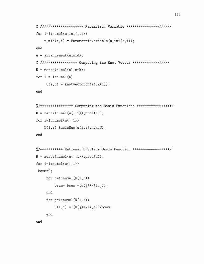
111
% //////*************** Parametric Variable ****************//////
for i=1:numel(u_ini(1,:))
u_mid(:,i) = ParametricVariable(u_ini(:,i));
end
u = arrangement(u_mid);
% /////************* Computing the Knot Vector *************/////
U = zeros(numel(n),n+k);
for i = 1:numel(n)
U(i,:) = knotvector(n(i),k(i));
end
%/**************** Computing the Basis Functions *****************/
N = zeros(numel(u(:,1)),prod(n));
for i=1:numel(u(:,1))
N(i,:)=BasisSum(u(i,:),n,k,U);
end
%/*********** Rational B-Spline Basis Function ******************/
R = zeros(numel(u(:,1)),prod(n));
for i=1:numel(u(:,1))
bsum=0;
for j=1:numel(N(1,:))
bsum= bsum +(w(j)*N(i,j));
end
for j=1:numel(N(1,:))
R(i,j) = (w(j)*N(i,j))/bsum;
end
end
112
% Computing the Control Points for the given Data Points or Surface
% Points.
p = ((R’)*R)\R’*P; % p - Resultant Control Points Vector
if numel(n) == 1
p(1,:) = P(1,:);
p(numel(p(:,1)),:) = P(numel(P(:,1)),:);
end
% for error
P_Test = nurbstest(p,u,n,k,w); % ’nurbstest2’ function is used to
% find the data points for the given control points
%Error
di = 0;
dif = zeros(1, numel(P(:,1)));
for j=1:(numel(P(:,1)))
dif(j)=((P(j,1)-P_Test(j,1))^2+(P(j,2)-P_Test(j,2))^2)^(1/2);
di= di + dif(j);
end
Error = di/(numel(P)/2);
end