Lecture 8 1

Optimizing CTL Model checking+

Model checking TCTL

CS 5270 Lecture 9

Lecture 8 2

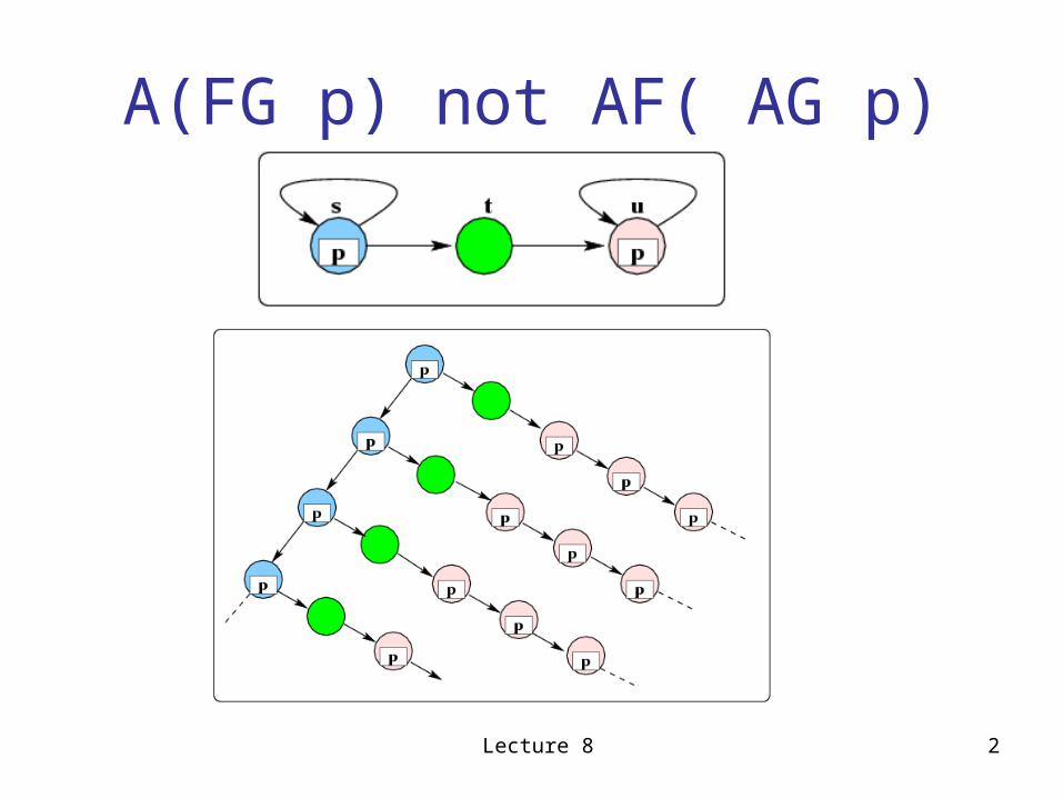
A(FG p) not AF( AG p)

Lecture 8 3

Today…

• Summary

• Optimizations for model checking– ROBDDs

• TCTL-– Syntax– Semantics– Algorithm for MC– Optimizations

Lecture 8 4

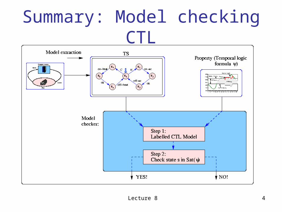
Summary: Model checking CTL

Lecture 8 5

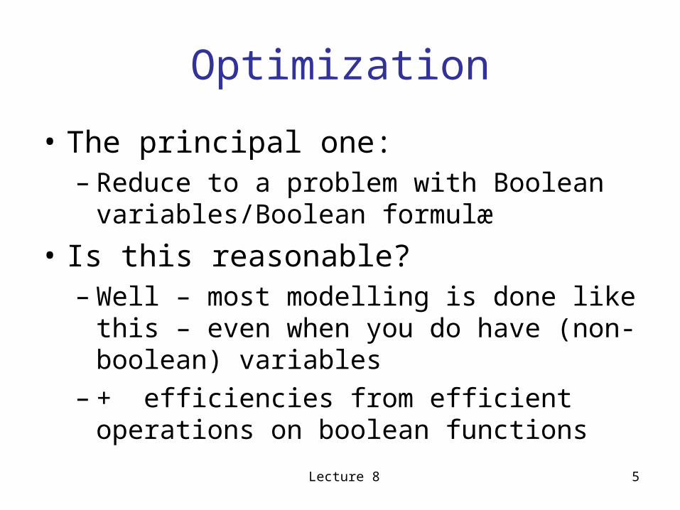
Optimization

• The principal one: – Reduce to a problem with Boolean

variables/Boolean formulæ

• Is this reasonable?– Well – most modelling is done like this – even

when you do have (non-boolean) variables– + efficiencies from efficient operations on

boolean functions

Lecture 8 6

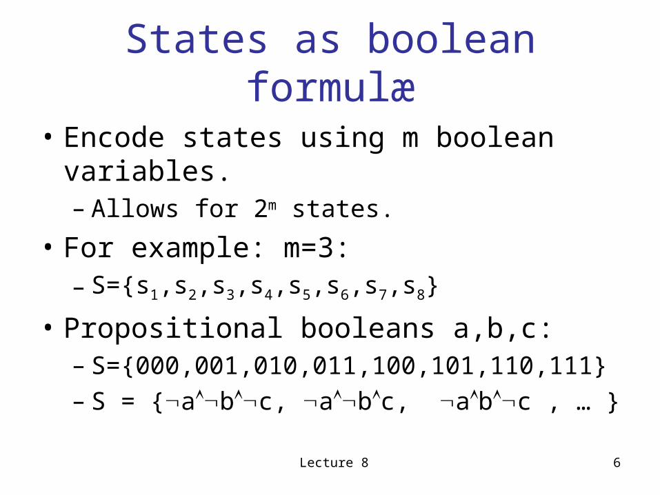
States as boolean formulæ

• Encode states using m boolean variables. – Allows for 2m states.

• For example: m=3: – S={s1,s2,s3,s4,s5,s6,s7,s8}

• Propositional booleans a,b,c:– S={000,001,010,011,100,101,110,111}– S = {abc, abc, abc , … }

Lecture 8 7

Transitions as boolean formulæ

• Encode (s,s’) using before and after propositional boolean variables– a,b,c and a’,b’,c’.

• For example: (s1,s4):

– (s1,s4) = (abc) (a’b’c’)

Lecture 8 8

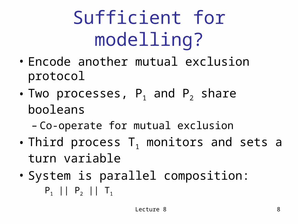
Sufficient for modelling?

• Encode another mutual exclusion protocol

• Two processes, P1 and P2 share booleans

– Co-operate for mutual exclusion

• Third process T1 monitors and sets a turn variable

• System is parallel composition:P1 || P2 || T1

Lecture 8 9

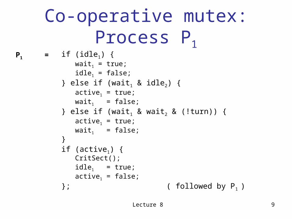
Co-operative mutex: Process P1

if (idle1) {wait1 = true;idle1 = false;

} else if (wait1 & idle2) {active1 = true;wait1 = false;

} else if (wait1 & wait2 & (!turn)) {active1 = true;wait1 = false;

}if (active1) {

CritSect();idle1 = true;active1 = false;

}; ( followed by P1 )

P1 =

Lecture 8 10

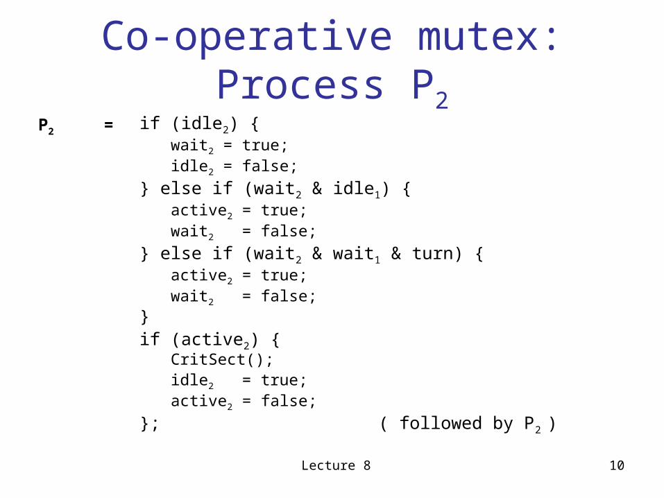
Co-operative mutex: Process P2

if (idle2) {wait2 = true;idle2 = false;

} else if (wait2 & idle1) {active2 = true;wait2 = false;

} else if (wait2 & wait1 & turn) {active2 = true;wait2 = false;

}if (active2) {

CritSect();idle2 = true;active2 = false;

}; ( followed by P2 )

P2 =

Lecture 8 11

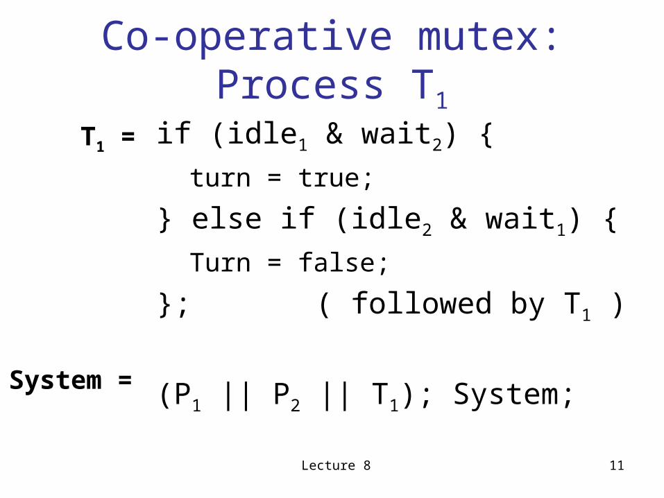
Co-operative mutex: Process T1

if (idle1 & wait2) {

turn = true;

} else if (idle2 & wait1) {

Turn = false;

}; ( followed by T1 )

(P1 || P2 || T1); System;

T1 =

System =

Lecture 8 12

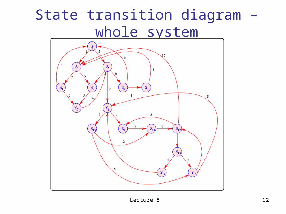
State transition diagram – whole system

Lecture 8 13

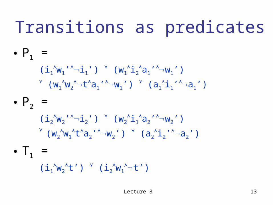
Transitions as predicates

• P1 = (i1w1’i1’) (w1i2a1’w1’)

(w1w2ta1’w1’) (a1i1’a1’)

• P2 = (i2w2’i2’) (w2i1a2’w2’)

(w2w1ta2’w2’) (a2i2’a2’)

• T1 = (i1w2t’) (i2w1t’)

Lecture 8 14

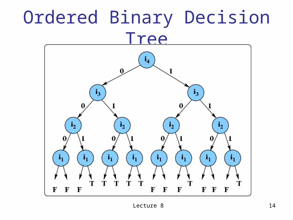
Ordered Binary Decision Tree

Lecture 8 15

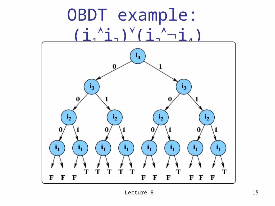
OBDT example: (i1i2)(i3i4)

Lecture 8 16

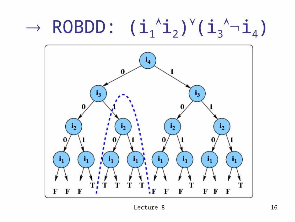
ROBDD: (i1i2)(i3i4)

Lecture 8 17

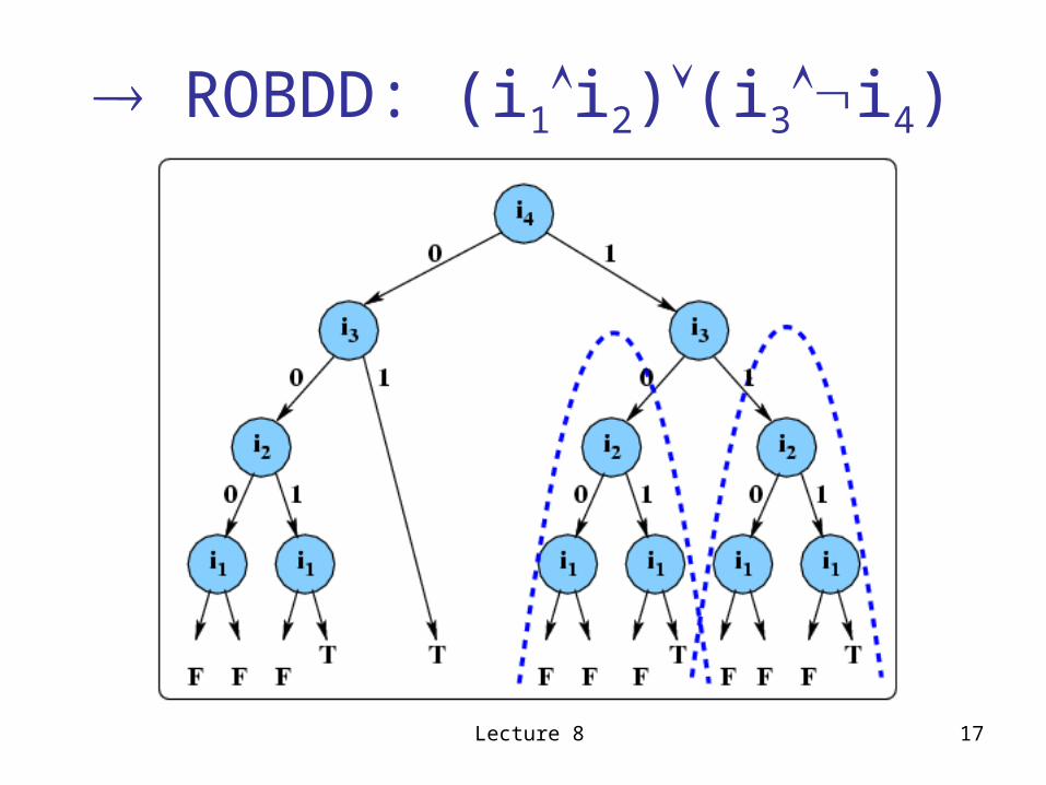
ROBDD: (i1i2)(i3i4)

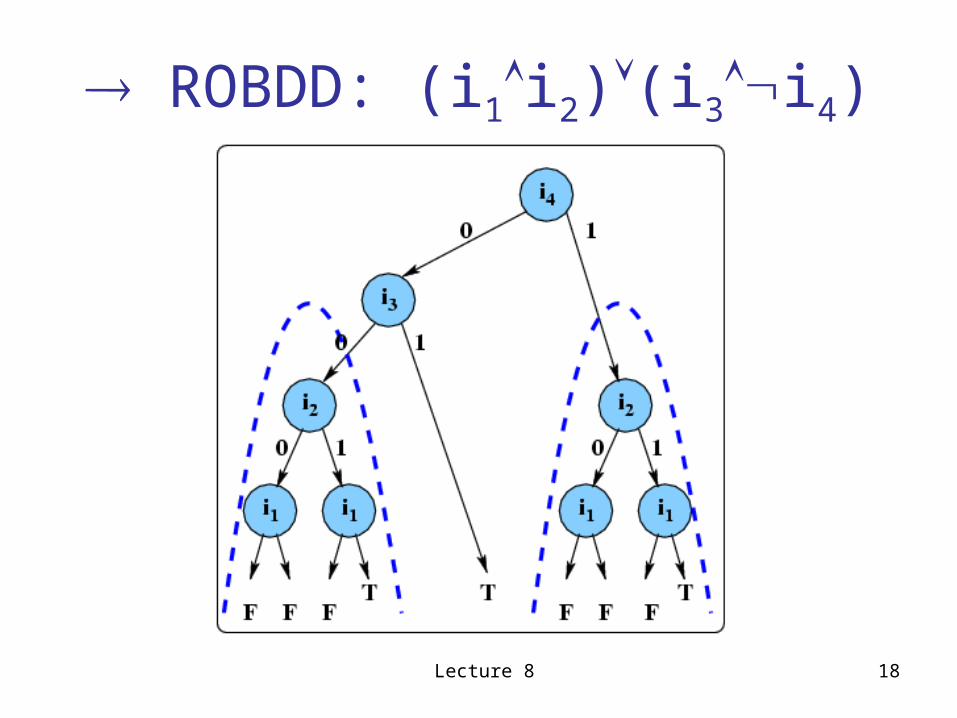
Lecture 8 18

ROBDD: (i1i2)(i3i4)

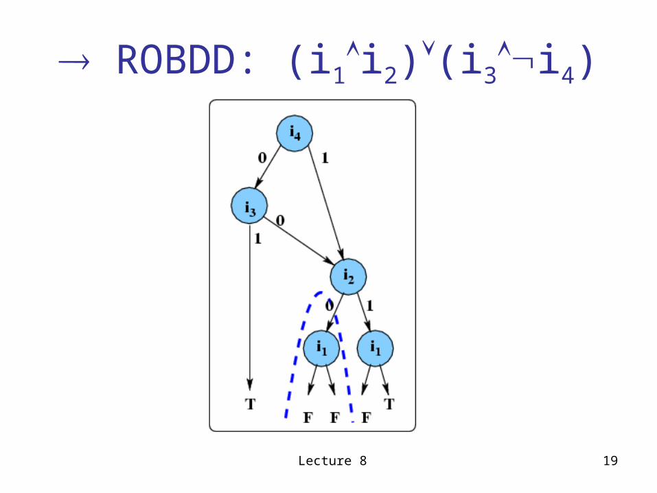
Lecture 8 19

ROBDD: (i1i2)(i3i4)

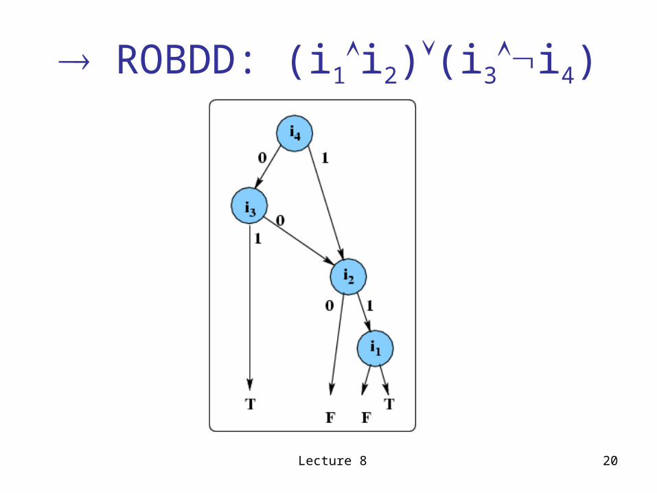
Lecture 8 20

ROBDD: (i1i2)(i3i4)

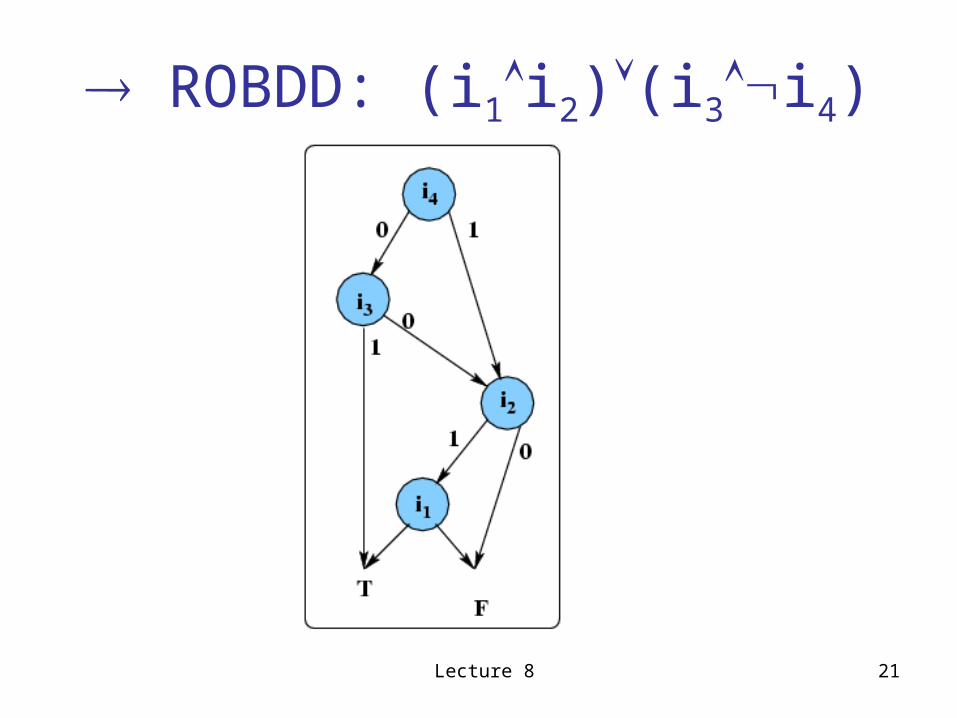
Lecture 8 21

ROBDD: (i1i2)(i3i4)

Lecture 8 22

History…

• The ROBDD optimization originally by Bryant (86) – paper on boolean graphs

• The application to model checking by McMillan (Originally in late 80’s – subject of thesis in 1992)

• smv – Symbolic model verifier – originally by McMillan

Lecture 8 23

Today…

• Summary

• Optimizations for model checking– ROBDDs

• TCTL-– Syntax– Semantics– Algorithm for MC– Optimizations

Lecture 8 24

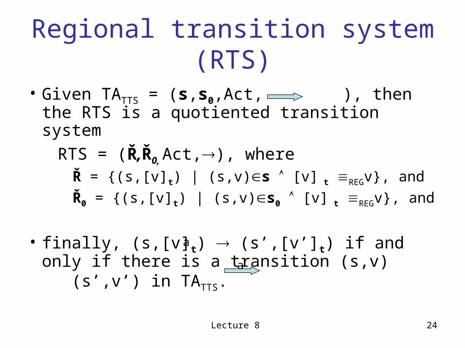
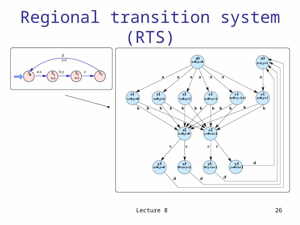
Regional transition system (RTS)

• Given TATTS = (s,s0,Act, ), then the RTS is a quotiented transition system

RTS = (Ř,Ř0, Act,), where Ř = {(s,[v]t) | (s,v)s [v] t REGv}, and

Ř0 = {(s,[v]t) | (s,v)s0 [v] t REGv}, and

• finally, (s,[v]t) (s’,[v’]t) if and only if there is a transition (s,v) (s’,v’) in TATTS.

a

a

Lecture 8 25

Regional transition system (RTS)

• Notation:Ř – a set of regions

ř – a particular region in the set: (s,[v]t)

r – a particular valuation: (s,v)

Lecture 8 26

Regional transition system (RTS)

Lecture 8 27

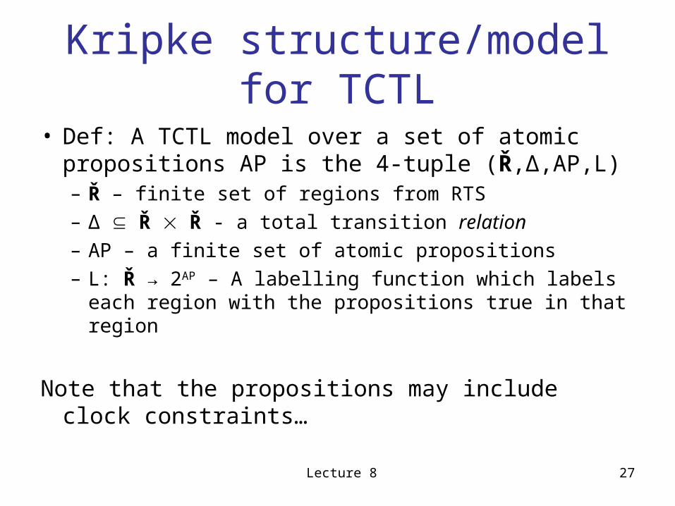
Kripke structure/model for TCTL

• Def: A TCTL model over a set of atomic propositions AP is the 4-tuple (Ř,Δ,AP,L) – Ř – finite set of regions from RTS– Δ Ř Ř - a total transition relation– AP – a finite set of atomic propositions– L: Ř → 2AP – A labelling function which labels each

region with the propositions true in that region

Note that the propositions may include clock constraints…

Lecture 8 28

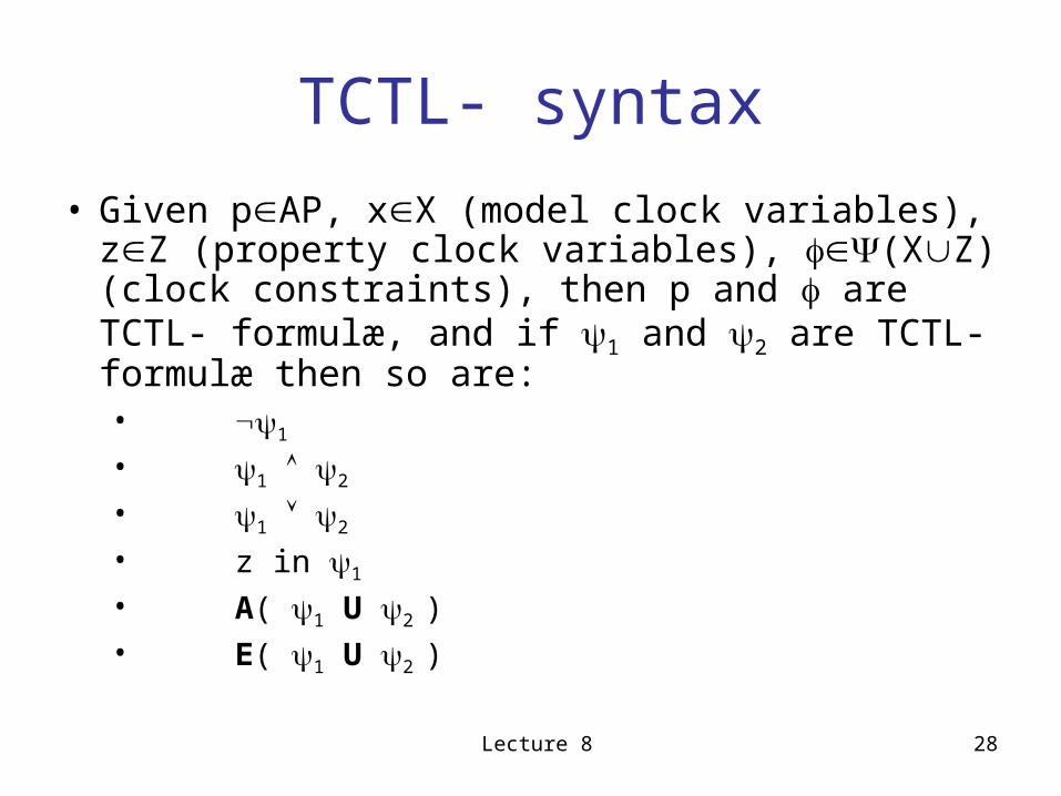
TCTL- syntax

• Given pAP, xX (model clock variables), zZ (property clock variables), (XZ) (clock constraints), then p and are TCTL- formulæ, and if 1 and 2 are TCTL- formulæ then so are:• 1

• 1 2

• 1 2

• z in 1

• A( 1 U 2 )• E( 1 U 2 )

Lecture 8 29

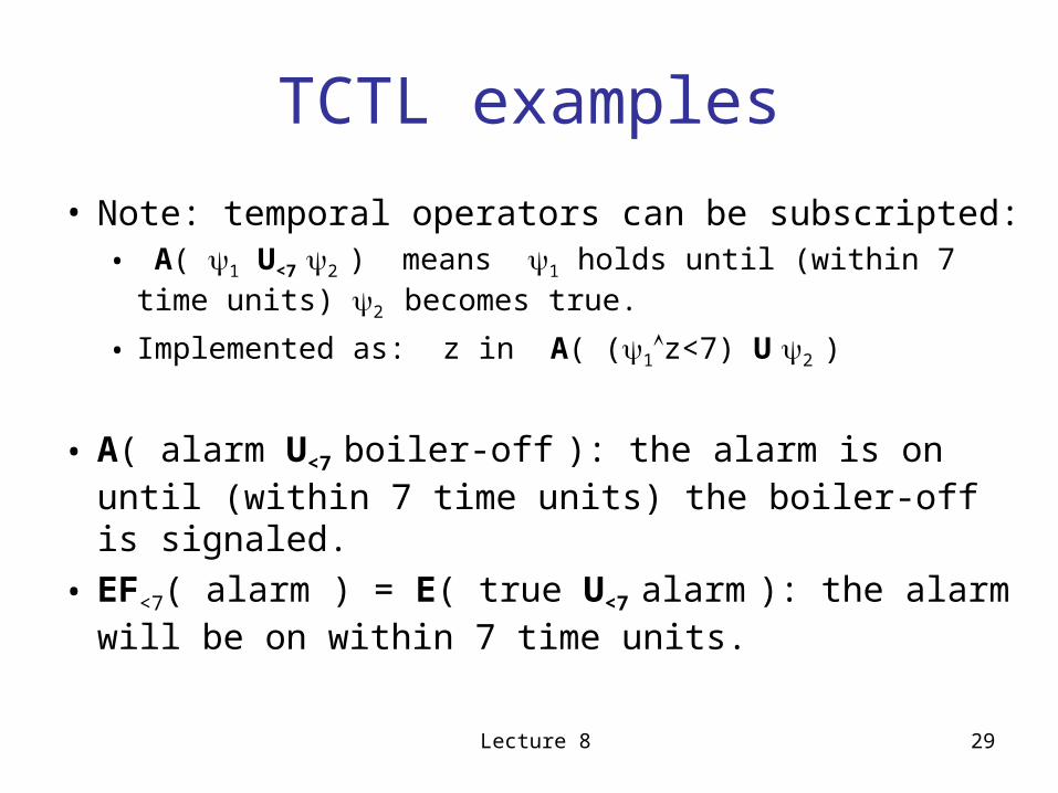
TCTL examples

• Note: temporal operators can be subscripted:• A( 1 U<7 2 ) means 1 holds until (within 7 time

units) 2 becomes true.

• Implemented as: z in A( (1z<7) U 2 )

• A( alarm U<7 boiler-off ): the alarm is on until (within 7 time units) the boiler-off is signaled.

• EF<7( alarm ) = E( true U<7 alarm ): the alarm will be on within 7 time units.

Lecture 8 30

Semantics of TCTL

• Expressed in terms of a model, and the modelling relation ² which links a model, a composite state r=(s,v) and a formula clock valuation with a property.

• M,(r,f) ² P - means that (TCTL) property P holds in (or is satisfied in) state r in the case of a formula valuation f for a given model M

Lecture 8 31

(Inductive) definition of ²

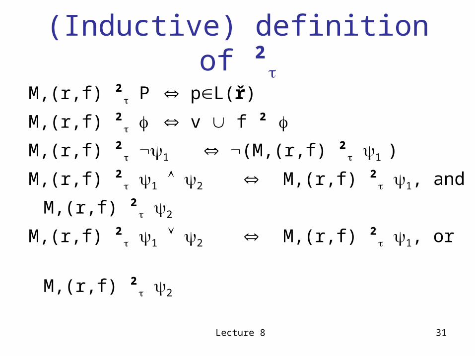
M,(r,f) ² P pL(ř)

M,(r,f) ² v f ²

M,(r,f) ² 1 (M,(r,f) ² 1 )

M,(r,f) ² 1 2 M,(r,f) ² 1, and

M,(r,f) ² 2

M,(r,f) ² 1 2 M,(r,f) ² 1, or

M,(r,f) ² 2

Lecture 8 32

(Inductive) definition of ²

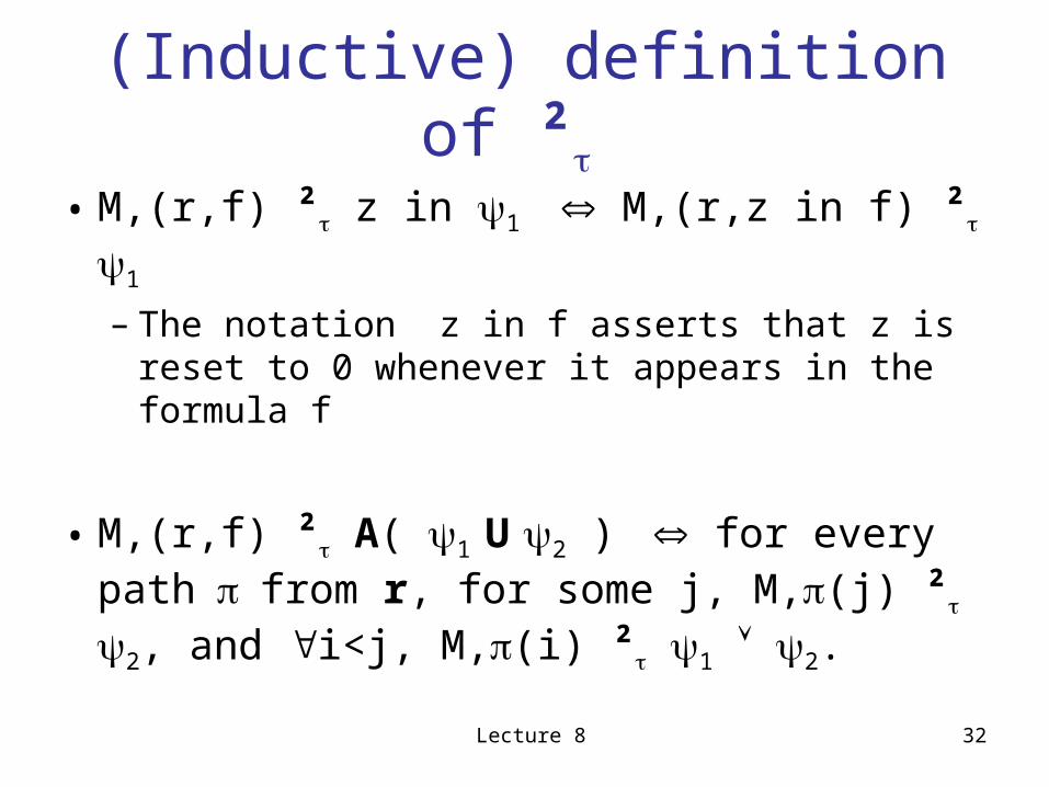
• M,(r,f) ² z in 1 M,(r,z in f) ² 1

– The notation z in f asserts that z is reset to 0 whenever it appears in the formula f

• M,(r,f) ² A( 1 U 2 ) for every pathfrom r, for some j, M,(j) ² 2, and i<j, M,(i) ² 1 2.

Lecture 8 33

(Inductive) definition of ²

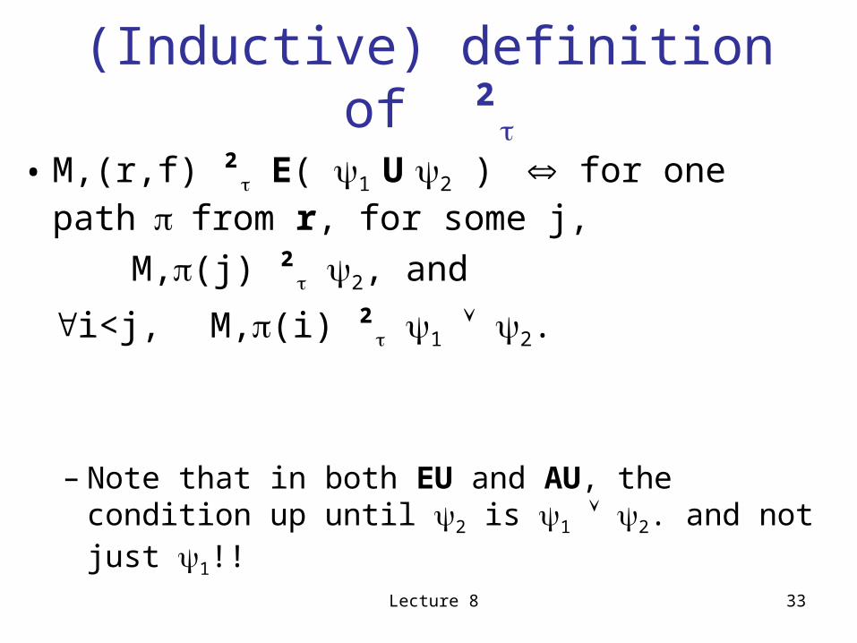
• M,(r,f) ² E( 1 U 2 ) for one pathfrom r, for some j,

M,(j) ² 2, and

i<j, M,(i) ² 1 2.

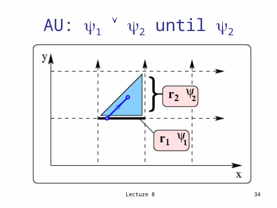
– Note that in both EU and AU, the condition up until 2 is 1 2. and not just 1!!

Lecture 8 34

AU: 1 2 until 2

Lecture 8 35

Model checking TCTL

• Definition of a labelling algorithm in the notes – not much different from CTL

• The only problem is this definition uses a least fixpoint iteration over an infinite set…

• In practice use the region construction…

Lecture 8 36

Optimization for TCTL MC

• We have already seen the steps to create a (finite) regional automaton

• Apart from that there is no magic bullet, and real-time model checking has an equivalent region-space explosion

• For this reason, limit the size of systems

• … so far …

Lecture 8 37

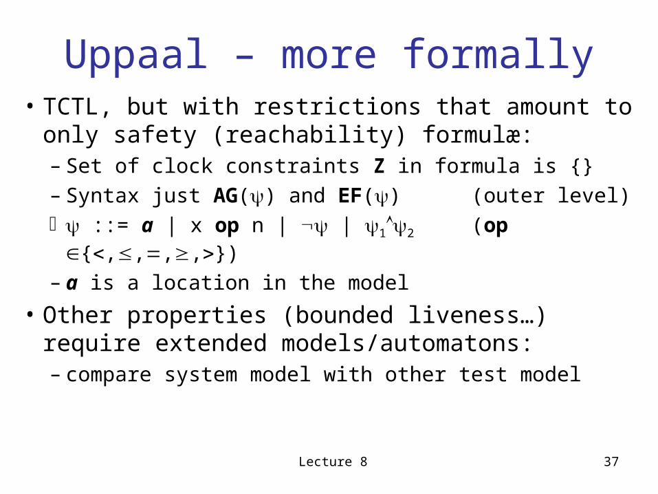
Uppaal – more formally• TCTL, but with restrictions that amount to only

safety (reachability) formulæ:– Set of clock constraints Z in formula is {}– Syntax just AG() and EF() (outer level) ::= a | x op n | | 12 (op {,,,,})

– a is a location in the model

• Other properties (bounded liveness…) require extended models/automatons:– compare system model with other test model