optimizing precision and power by machine learning in
TRANSCRIPT

arX
iv:2
109.
0429
4v1
[st
at.M
E]
9 S
ep 2
021
Optimizing Precision and Power by Machine Learning
in Randomized Trials, with an Application to
COVID-19
Nicholas Williams1, Michael Rosenblum2, and Iván Díaz∗1
1Division of Biostatistics, Department of Population Health Sciences, Weill Cornell Medicine.2Department of Biostatistics, Johns Hopkins Bloomberg School of Public Health.
September 10, 2021
Abstract
The rapid finding of effective therapeutics requires the efficient use of available re-sources in clinical trials. The use of covariate adjustment can yield statistical estimateswith improved precision, resulting in a reduction in the number of participants requiredto draw futility or efficacy conclusions. We focus on time-to-event and ordinal outcomes.When more than a few baseline covariates are available, a key question for covariateadjustment in randomized studies is how to fit a model relating the outcome and thebaseline covariates to maximize precision. We present a novel theoretical result estab-lishing conditions for asymptotic normality of a variety of covariate-adjusted estimatorsthat rely on machine learning (e.g., ℓ1-regularization, Random Forests, XGBoost, andMultivariate Adaptive Regression Splines), under the assumption that outcome datais missing completely at random. We further present a consistent estimator of theasymptotic variance. Importantly, the conditions do not require the machine learningmethods to converge to the true outcome distribution conditional on baseline variables,as long as they converge to some (possibly incorrect) limit. We conducted a simula-tion study to evaluate the performance of the aforementioned prediction methods inCOVID-19 trials using longitudinal data from over 1,500 patients hospitalized withCOVID-19 at Weill Cornell Medicine New York Presbyterian Hospital. We found thatusing ℓ1-regularization led to estimators and corresponding hypothesis tests that con-trol type 1 error and are more precise than an unadjusted estimator across all samplesizes tested. We also show that when covariates are not prognostic of the outcome,ℓ1-regularization remains as precise as the unadjusted estimator, even at small samplesizes (n = 100). We give an R package adjrct that performs model-robust covariateadjustment for ordinal and time-to-event outcomes.
∗corresponding author: [email protected]
1

1 Introduction
Coronavirus disease 2019 (COVID-19) has affected more than 125 million people and causedmore than 2.7 million deaths worldwide (World Health Organization 2021). Governmentsand scientists around the globe have deployed an enormous amount of resources to combatthe pandemic with remarkable success, such as the development in record time of highly effec-tive vaccines to prevent disease (e.g., Polack et al. 2020; Baden et al. 2021). Global and localorganizations are launching large-scale collaborations to collect robust scientific data to testpotential COVID-19 treatments, including the testing of drugs re-purposed from other dis-eases as well as new compounds (Kupferschmidt and Cohen 2020). For example, the WorldHealth Organization launched the SOLIDARITY trial, enrolling almost 12,000 patients in500 hospital sites in over 30 countries (WHO Solidarity Trial Consortium 2021). Other largeinitiatives include the RECOVERY trial (The RECOVERY Collaborative Group 2021) andthe ACTIV initiative (Collins and Stoffels 2020). To date, there are approximately 2,400randomized trials for the treatment of COVID-19 registered in clinicaltrials.gov.
The rapid finding of effective therapeutics for COVID-19 requires the efficient use ofavailable resources. One area where such efficiency is achievable at little cost is in the statis-tical design and analysis of the clinical trials. Specifically, a statistical technique known ascovariate adjustment may yield estimates with increased precision (compared to unadjustedestimators), and may result in a reduction of the time, number of participants, and resourcesrequired to draw futility or efficacy conclusions. This results in faster trial designs, whichmay help accelerate the delivery of effective treatments to patients who need them (and mayhelp rule out ineffective treatments faster).
Covariate adjustment refers to pre-planned analysis methods that use data on patientbaseline characteristics to correct for chance imbalances across study arms, thereby yieldingmore precise treatment effect estimates. The ICH E9 Guidance on Statistical Methods forAnalyzing Clinical Trials (FDA and EMA 1998) states that “Pretrial deliberations shouldidentify those covariates and factors expected to have an important influence on the primaryvariable(s), and should consider how to account for these in the analysis to improve precisionand to compensate for any lack of balance between treatment groups.” Even though itsbenefits can be substantial, covariate adjustment is underutilized; only 24%-34% of trialsuse covariate adjustment (Kahan et al. 2014).
We focus on estimation of marginal treatment effects, defined as a contrast betweenstudy arms in the marginal distribution of the outcome. Many approaches for estima-tion of marginal treatment effects using covariate adjustment in randomized trials invokea model relating the outcome and the baseline covariates within strata of treatment. Re-cent decades have seen a surge in research on the development of model-robust methods forestimating marginal effects that remain consistent even if this outcome regression model isarbitrarily misspecified (e.g., Yang and Tsiatis 2001; Tsiatis et al. 2008; Zhang et al. 2008;Moore and van der Laan 2009a; Austin et al. 2010; Zhang and Gilbert 2010; Benkeser et al.2020). We focus on a study of the model-robust covariate adjusted estimators for time-to-event and ordinal outcomes developed by Moore and van der Laan (2009a), Díaz et al.(2019), and Díaz et al. (2016).
All potential adjustment covariates must be pre-specified in the statistical analysis plan.At the end of the trial, a prespecified prediction algorithm (e.g., random forests, or using
2

regularization for variable selection) will be run and its output used to construct a model-robust, covariate adjusted estimator of the marginal treatment effect for the trial’s primaryefficacy analysis. We aim to address the question of how to do this in a model-robust way thatguarantees consistency and asymptotic normality, under some weaker regularity conditionsthan related work (described below). We also aim to demonstrate the potential value addedby covariate adjustment combined with machine learning, through a simulation study basedon COVID-19 data.
As a standard regression method for high-dimensional data, ℓ1-regularization has beenstudied by several authors in the context of covariate selection for randomized studies. Forexample, Wager et al. (2016) present estimators that are asymptotically normal under strongassumptions that include linearity of the outcome-covariate relationship. Bloniarz et al.(2016) present estimators under a randomization inference framework, and show asymptoticnormality of the estimators under assumptions similar to the assumptions made in this paper.Both of these papers present results only for continuous outcomes. The method of Tian et al.(2012) is general and can be applied to continuous, ordinal, binary, and time-to-event data,and its asymptotic properties are similar to the properties of the methods we discuss for thecase of ℓ1-regularization, under similar assumptions.
More related to our general approach, Wager et al. (2016) also present a cross-validationprocedure that can be used with arbitrary non-parametric prediction methods (e.g., ℓ1-regularization, random forests, etc.) in the estimation procedure. Their proposal amounts tocomputation of a cross-fitted augmented inverse probability weighted estimator (Chernozhukov et al.2018). Their asymptotic normality results, unlike ours, require that that their predictor of theoutcome given baseline variables converges to the true regression function. Wu and Gagnon-Bartsch(2018) proposed a “leave-one-out-potential outcomes” estimator where automatic predictioncan also be performed using any regression procedure such as linear regression or randomforests, and they propose a conservative variance estimator. It is unclear as of yet whetherWald-type confidence intervals based on the normal distribution are appropriate for thisestimator. As in the above related work that compares the precision of covariate adjustedestimators to the unadjusted estimator, we assume that outcomes are missing completely atrandom (since otherwise the unadjusted estimator is generally inconsistent).
In Section 3.3, we present our main theorem. It shows that any of a large class ofprediction algorithms (e.g., ℓ1-regularization, Random Forests, XGBoost, and MultivariateAdaptive Regression Splines) can be combined with the covariate adjusted estimator ofMoore and van der Laan (2009b) to produce a consistent, asymptotically normal estimatorof the marginal treatment effect, under regularity conditions. These conditions do not requireconsistent estimation of the outcome regression function (as in key related work describedabove); instead, our theorem requires the weaker condition of convergence to some (possiblyincorrect) limit. We also give a consistent, easy to compute variance estimator. This hasimportant practical implications because it allows the use machine learning coupled withWald-type confidence intervals and hypothesis tests, under the conditions of the theorem.The above estimator can be used with ordinal or time-to-event outcomes.
We next conduct a simulation study to evaluate the performance of the aforementionedmachine learning algorithms for covariate adjustment in the context of COVID-19 trials. Wesimulate two-arm trials comparing a hypothetical COVID-19 treatment to standard of care.The simulated data distributions are generated from longitudinal data on approximately
3

1,500 patients hospitalized at Weill Cornell Medicine New York Presbyterian Hospital priorto 15 May 2020. We present results for two types of endpoints: time-to-event (e.g., time tointubation or death) and ordinal (e.g., WHO scale, see Marshall et al. 2020) outcomes. Forsurvival outcomes, we present results for two different estimands (i.e., targets of inference):the survival probability at any given time and the restricted mean survival time. For ordi-nal outcomes we present results for the average log-odds ratio, and for the Mann-Whitneyestimand, interpreted as the probability that a randomly chosen treated patient has a betteroutcome than a randomly chosen control patient (with ties broken at random).
Benkeser et al. (2020) used simulations based on the above data source to illustratethe efficiency gains achievable by covariate adjustment with parametric models includinga small number of adjustment variables (and not using machine learning to improve effi-ciency). In this paper we evaluate the performance of four machine learning algorithms (ℓ1-regularization, Random Forests, XGBoost, and Multivariate Adaptive Regression Splines)in several sample sizes, and compare them in terms of their bias, mean squared error, andtype-1 and type-2 errors, to unadjusted estimators and to fully adjusted main terms logisticregression with all available variables included. Furthermore, we introduce a new R pack-age adjrct (Díaz and Williams 2021) that can be used to perform model-robust covariateadjustment for ordinal and time-to-event outcomes, and provide R code that can be used toreplicate our simulation analyses with other data sources.
2 Estimands
In what follows, we focus on estimating intention-to-treat effects and refer to study armassignment simply as treatment. We focus on estimation of marginal treatment effects,defined as a contrast between study arms in the marginal distribution of the outcome. Wefurther assume that we have data on n trial participants, represented by n independent andidentically distributed copies of data Oi : i = 1, . . . , n. We assume Oi is distributed asP, where we make no assumptions about the functional form of P except that treatmentis independent of baseline covariates (by randomization). We denote a generic draw fromthe distribution P by O. We use the terms “baseline covariate” and “baseline variable”interchangeably to indicate a measurement made before randomization.
We are interested in making inferences about a feature of the distribution P. We use theword estimand to refer to such a feature. We describe example estimands, which includethose used in our simulations studies, below.
2.1 Ordinal Outcomes
For ordinal outcomes, assume the observed data is O = (W,A, Y ), where W is a vector ofbaseline covariates, A is the treatment arm, and Y is an ordinal variable that can take valuesin {1, . . . , K}. Let F (k, a) = P(Y ≤ k | A = a) denote the cumulative distribution functionfor patients in arm A = a, and let f(k, a) = F (k, a)− F (k − 1, a) denote the correspondingprobability mass function. For notational convenience we will sometimes use the “survival”
4

function instead: S(k, a) = 1− F (k, a). The average log-odds ratio is then equal to
LOR =1
K − 1
K−1∑
k=1
log
[F (k, 1)/{1− F (k, 1)}F (k, 0)/{1− F (k, 0)}
],
and the Mann-Whitney estimand is equal to
MW =
K∑
k=1
{F (k − 1, 0) +
1
2f(k, 0)
}f(k, 1).
The Mann-Whitney estimand can be interpreted as the probability that a randomly drawnpatient from the treated arm has a better outcome than a randomly drawn patient fromthe control arm, with ties broken at random (Ahmad 1996). The average log-odds ratio ismore difficult to interpret and we discourage its use, but we include it in our comparisonsbecause it is a non-parametric extension of the parameter β estimated by the commonlyused proportional odds model logit{F (k, a)} = αk + βa (Díaz et al. 2016).
2.2 Time to Event Outcomes
For time to event outcomes, we assume the observed data is O = (W,A,∆ = 1{Y ≤ C}, Y =min(C, Y )), where C is a right-censoring time denoting the time that a patient is last seen,and 1{E} is the indicator variable taking the value 1 on the event E and 0 otherwise. Wefurther assume that events are observed at discrete time points {1, . . . , K} (e.g., days) as istypical in clinical trials. The difference in restricted mean survival time is given by
RMST =K−1∑
k=1
{S(k, 1)− S(k, 0)},
and can be interpreted as a contrast comparing the expected survival time within thefirst K time units for the treated arm minus the control arm (Chen and Tsiatis 2001;Royston and Parmar 2011). The risk difference at a user-given time point k is defined as
RD = S(k, 1)− S(k, 0),
and is interpreted as the difference in survival probability for a patient in the treated armminus the control arm. We note that the MW and RD parameters may be meaningful forboth ordinal and time-to-event outcomes.
3 Estimators
For the sake of generality, in what follows we use a common data structure O = (W,A,∆ =
1{Y ≤ C}, Y ) for both ordinal and survival outcomes, where for ordinal outcomes C = Kif the outcome is observed and C = 0 if it is missing.
Many approaches for estimation of marginal treatment effects using covariate adjustmentin randomized trials invoke a model relating the outcome and the baseline covariates within
5

strata of treatment. It is important that the consistency and interpretability of the treatmenteffect estimates do not rely on the ability to correctly posit such a model. Specifically, in arecent draft guidance (U.S. Food and Drug Administration 2021), the FDA states: “Sponsorscan perform covariate adjusted estimation and inference for an unconditional treatment effect... in the primary analysis of data from a randomized trial. The method used should providevalid inference under approximately the same minimal statistical assumptions that wouldbe needed for unadjusted estimation in a randomized trial.” The assumption of a correctlyspecified model is not typically part of the assumptions needed for an unadjusted analysis,and should therefore be avoided when possible.
All estimands described in this paper can be computed from the cumulative distributionfunctions (CDF) F (·, a) for a ∈ {0, 1}, which can be estimated using the empirical cumulativedistribution function (ECDF) or the Kaplan-Meier estimator. Model-robust, covariate ad-justed estimators have been developed for the CDF, including, e.g., Chen and Tsiatis (2001);Rubin and van der Laan (2008); Moore and van der Laan (2009b); Stitelman et al. (2011);Lu and Tsiatis (2011); Brooks et al. (2013); Zhang (2014); Parast et al. (2014); Benkeser et al.(2018); Díaz (2019).
We focus on the model-robust, covariate adjusted estimators of Moore and van der Laan(2009b), Díaz et al. (2016), and Díaz et al. (2019). These estimators have at least two ad-vantages compared to unadjusted estimators based on the ECDF or the Kaplan-Meier esti-mator. First, with time-to-event outcomes, the adjusted estimator can achieve consistencyunder an assumption of censoring being independent of the outcome given study arm andbaseline covariates (C ⊥⊥ Y |A,W ), rather than the assumption of censoring in each armbeing independent of the outcome marginally (C ⊥⊥ Y |A) required by unadjusted estima-tors. The former assumption is arguably more likely to hold in typical situations wherepatients are lost to follow-up due to reasons correlated with their baseline variables. Sec-ond, in large samples and under regularity conditions, the adjusted estimators of Díaz et al.(2016) and Díaz et al. (2019) can be at least as precise as the unadjusted estimator (this re-quires that missingness/censoring is completely at random, i.e., that in each arm a ∈ {0, 1},C ⊥⊥ (Y,W )|A = a), under additional assumptions.
Additionally, under regularity conditions, the three aforementioned adjusted estimatorsare asymptotically normal. This allows the construction of Wald-type confidence intervalsand corresponding tests of the null hypothesis of no treatment effect.
3.1 Prediction algorithms
While we make no assumption on the functional form of the distribution P (except thattreatment is independent of baseline variables by randomization), implementation of ourestimators requires a working model for the following conditional probability
m(k, a,W ) = P(Y = k,∆ = 1 | Y ≥ k, A = a,W ).
In time-to-event analysis, this probability is known as the conditional hazard. The expres-sion working model here means that we do not assume that the model represents the truerelationship between the outcome and the treatment/covariates. Fitting a working modelfor m is equivalent to training a prediction model for m (specifically, a prediction model for
6

the probability of Y = k,∆ = 1 given Y ≥ k, A = a,W ), and we sometimes refer to themodel fit as a predictor.
In our simulation studies, we will use the following working models, fitted in a datasetwhere each participant contributes a row of data corresponding to each time k = 1 throughk = Y :
• The following pooled main terms logistic regression (LR) logit{mβ(k, a,W )} = βa,0,k+β⊤
a,1W estimated with maximum likelihood estimation. Note that this model has (i)separate parameters for each study arm, and (ii) in each arm, intercepts for eachpossible outcome level k.
• The above model fitted with an ℓ1 penalty on the parameter βa,1 (ℓ1-LR, Tibshirani1996; Park and Hastie 2007).
• A random forest classification model (RF, Breiman 2001).
• An extreme gradient boosting tree ensemble (XGBoost, Friedman 2001).
• Multivariate adaptive regression splines (MARS, Friedman 1991).
For RF, XGBoost, and MARS, the algorithms are trained in the whole sample {1, . . . , n}.For these algorithms, we also assessed the performance of cross-fitted versions of the esti-mators. Cross-fitting is sometimes necessary to guarantee that the regularity assumptionsrequired for asymptotic normality of the estimators hold when using data-adaptive regres-sion methods (Klaassen 1987; Zheng and van der Laan 2011; Chernozhukov et al. 2018),and is performed as follows. Let V1, . . . ,VJ denote a random partition of the index set{1, . . . , n} into J prediction sets of approximately the same size. That is, Vj ⊂ {1, . . . , n};⋃J
j=1 Vj = {1, . . . , n}; and Vj∩Vj′ = ∅. In addition, for each j, the associated training sampleis given by Tj = {1, . . . , n}\Vj. Let mj denote the prediction algorithm trained in Tj . Lettingj(i) denote the index of the prediction set which contains observation i, cross-fitting entailsusing only observations in Tj(i) for fitting models when making predictions about observationi. That is, the outcome predictions for each subject i are given by mj(i)(u, a,Wi). We letηj(i) = (mj(i), πA, πC) for cross-fitted estimators and ηj(i) = (m, πA, πC) for non-cross-fittedones. RF, XGBoost, and MARS were fit using the ranger (Wright and Ziegler 2017), xgboost(Chen et al. 2021), and earth (Milborrow 2020) R packages, respectively. Hyperparametertuning was performed using cross-validation with the origami (Coyle and Hejazi 2020) Rpackage.
3.2 Targeted minimum loss based estimation (TMLE)
Our simulation studies use the TMLE procedure presented in Díaz et al. (2019). We will referto that estimator as TMLE with improved efficiency, or IE-TMLE. We will first present theTMLE of (Moore and van der Laan 2009b), which constitutes the basis for the constructionof the IE-TMLE.
In the supplementary materials we present some of the efficiency theory underlying theconstruction of the TMLE. Briefly, TMLE is a framework to construct estimators ηj(i) thatsolve the efficient influence function estimating equation n−1
∑ni=1Dηj(i)(Oi) = 0, where
7

Dη(O) is the efficient influence function for S(k, a) in the non-parametric model that onlyassumes treatment A is independent of baseline variables W (which holds by design), definedin the supplementary materials. TMLE enjoys desirable properties such as local efficiency,outcome model robustness under censoring completely at random, and asymptotic normality,under regularity assumptions.
TMLE estimator definition: Given a predictor m constructed as in the previoussubsection and any k, a, the corresponding TMLE estimation procedure for F (k, a) can besummarized in the next steps:
1. Create a long-form dataset where each participant i contributes the following row ofdata corresponding to each time u = 0 through k:
(u,Wi, Ai, 1{Y ≥ u}, 1{Y = u,∆ = 0}, 1{Y = u,∆ = 1}
),
where 1{X} is the indicator variable taking value 1 if X is true and 0 otherwise.
2. For each individual i, obtain a prediction m(u, a,Wi) for each pair in the set {(u, a) :a = 0, 1; u = 0, . . . , k}.
3. Fit a model πA(a,W ) for the probability P(A = a | W ). Note that, in randomizedtrials, this model may be correctly specified by a logistic regression logit πA(1,W ) =α0 + α⊤
1 W . Let πA(a,Wi) denote the prediction of the model for individual i.
4. Fit a model πC(u, a,W ) for the censoring probabilities P(Y = u,∆ = 0 | Y ≥ u,A =a,W ). For time-to-event outcomes, this is a model for the censoring probabilities. Forordinal outcomes, the only possibilities are that C = 0 (outcome missing) or C = K(outcome observed); in this case we only fit the aforementioned model at u = 0 and weset πC(u, a,W ) = 0 for each u > 0. For either outcome type, if there is no censoring(i.e., if P (∆ = 1) = 1), then we set πC(u, a,W ) = 0 for all u. Let πC(u, a,Wi) denotethe prediction of this model for individual i, i.e., using the baseline variable valuesfrom individual i.
5. For each individual i and each u ≤ k, compute a “clever” covariate HY,k,u as a functionof m, πA, and πC as detailed in the supplementary materials. The outcome model fitm is then updated by fitting the following logistic regression “tilting" model with singleparameter ǫ and offset based on m:
P(Y = u,∆ = 1 | Y ≥ u,A = a,W ) = logit−1 {logit m(u, a,W ) + εHY,k,u} .
This can be done using standard statistical software for fitting a logistic regression ofthe indicator variable 1{Y = u,∆ = 1} on the variable HY,k,u using offset logit m(u, a,W )
among observations with Y ≥ u and A = a in the long-form dataset from step 1. Theabove model fitting process is iterated where at the beginning of each iteration wereplace m in the above display and in the definition of HY,k,u by the updated modelfit. We denote the maximum number of iterations that we allow by imax.
8

6. Let m(u, a,Wi) denote the estimate of m(u, a,Wi) for individual i at the final itera-tion of the previous step. Note that this estimator is specific to the value k underconsideration.
7. Compute the estimate of S(k, a) = 1−F (k, a) as the following standardized estimator
STMLE(k, a) =1
n
n∑
i=1
k∏
u=1
{1− m(u, a,Wi)}, (1)
and let the estimator of F (k, a) be 1− STMLE(k, a).
This estimator was originally proposed by Moore and van der Laan (2009b). The role of
the clever covariate HY,k,u is to endow the resulting estimator S(k, a) with properties suchas model-robustness compared to unadjusted estimators. In particular, it can be shownthat this estimator is efficient when the working model for m is correctly specified. Thespecific form of the covariate HY,k,u is given in the supplementary materials. Throughout,the notation m is used to represent the predictor constructed as in Section 3.1 and whichis an input to the above TMLE algorithm, while m denotes the updated version of thispredictor that is output by the above TMLE algorithm at step 6.
IE-TMLE estimator definition: In Section 4 we will compare several machine learningprocedures for estimating m in finite samples. The estimators used in the simulation studyare the IE-TMLE of Díaz et al. (2019), where in addition to updating the initial estimatorfor the outcome regression m, we also update the estimators of the treatment and censoringmechanisms. Specifically, we replace step 5 of the above procedure with the following:
5. For each individual i construct “clever” covariates HY,k,u, HA, and HC,k,u (defined inthe supplementary materials) as a function of m, πA, and πC . For each k = 1, . . . , K,the model fits are then iteratively updated using logistic regression “tilting" models:
logitmε(u, a,W ) = logit m(u, a,W ) + εHY,k,u
logitπγ,A(1,W ) = logit πA(1,W ) + γHA
logit πυ,C(u, a,W ) = logit πC(u, a,W ) + υHC,k,u
where the iteration is necessary because HY,k,u, HA, and HC,k,u are functions of m, πA,and πC that must be updated at each step. As before, for ordinal outcomes we onlyfit the aforementioned model at u = 0 and we set πC(u, a,W ) = 0 for each u > 0.
We use SIE−TMLE to denote this estimator. The updating step above combines ideas fromMoore and van der Laan (2009b), Gruber and van der Laan (2012), and Rotnitzky et al.(2012) to produce an estimator with the following properties:
(i) Consistency and at least as precise as the Kaplan-Meier and inverse probability weightedestimators;
(ii) Consistency under violations of independent censoring (unlike the Kaplan-Meier esti-mator) when either the censoring or survival distributions, conditional on covariates,are estimated consistently and censoring is such that C ⊥⊥ Y | W,A; and
9

(iii) Nonparametric efficiency when both of these distributions are consistently estimatedat rate n1/4.
Please see Díaz et al. (2019) for more details on these estimators, which are implemented inthe R package adjrct (Díaz and Williams 2021).
Next, we present a result (Theorem 1) stating asymptotic normality of STMLE usingmachine learning for prediction that avoids some limitations of existing methods, and presenta consistent estimator of its variance. In Section 4 we present simulation results wherewe evaluate the performance of SIE−TMLE for covariate adjustment in COVID-19 trials forhospitalized patients. We favor SIE−TMLE in our numerical studies because, unlike STMLE,it satisfies property (i) above. The simulation uses Wald-type hypothesis tests based on theasymptotic approximation of Theorem 1, where we note that the variance estimator in thetheorem is consistent for STMLE but it is conservative for SIE−TMLE (Moore and van der Laan2009b).
3.3 Asymptotically correct confidence intervals and hypothesis testsfor TMLE combined with machine learning
Most available methods to construct confidence intervals and hypothesis tests in the statisticsliterature are based on the sampling distribution of the estimator. While using the exactfinite-sample distribution would be ideal for this task, such distributions are notoriouslydifficult to derive for our problem in the absence of strong and unrealistic assumptions(such as linear models with Gaussian noise). Thus, here we focus on methods that rely onapproximating the finite-sample distribution using asymptotic results as n goes to infinity.
In order to discuss existing methods, it will be useful to introduce and compare thefollowing assumptions:
A1. Censoring is completely at random, i.e., C ⊥⊥ (Y,W ) | A = a for each treatment arm a.
A2. Let ||f ||2 denote the L2(P) norm∫f 2(o)dP(o), for O = (W,A,∆ = 1{Y ≤ C}, Y ). We
abbreviate m(k, a,W ) and m(k, a,W ) by m and m, respectively. Assume the estimator mis consistent in the sense that ||m−m|| = oP (1) for all k ∈ {1, . . . , K} and a ∈ {0, 1}. Wealso assume that there exists a δ > 0 such that δ < m < 1− δ with probability 1.
A3. Assume the estimator m converges to a possibly misspecified limit m1 in the sense that||m−m1|| = oP (1) for all k ∈ {1, . . . , K} and a ∈ {0, 1}, where we emphasize that m1 canbe different from the true regression function m. We also assume that there exists a δ > 0such that δ < m1 < 1− δ with probability 1.
For estimators m of m that use cross-fitting, the function m consists of J maps (one foreach training set) from the sample space of O to the interval [0, 1]. In this case, by conventionwe define ||m−m|| in A2 as the average across the J maps of the L2(P) norm of each suchmap minus m. Convergence of ||m−m|| to 0 in probability is then equivalent to the sameconvergence where m is replaced by the corresponding map before cross-fitting is applied.The same convention is used in A3.
There are at least two results on asymptotic normality for STMLE relevant to the prob-lem we are studying. The first result is a general theorem for TMLE (see Appendix A.1 of
10

van der Laan and Rose 2011), stating that the estimator is asymptotically normal and effi-cient under regularity assumptions which include A2. Among other important implications,this asymptotic normality implies that the variance of the estimators can be consistentlyestimated by the empirical variance of the efficient influence function. This means thatasymptotically correct confidence intervals and hypothesis tests can be constructed using aWald-type procedure. As stated above, it is often undesirable to assume A2 in the settingof a randomized trial, as it is a much stronger assumption than what would be required foran unadjusted estimator.
The second result of relevance to this paper establishes asymptotic normality of S(k, a)under assumptions that include A3 (Moore and van der Laan 2009a). The asymptotic vari-ance derived by these authors depends on the true outcome regression function m, and isthus difficult to estimate. As a solution, the authors propose to use a conservative estimateof the variance whose computation does not rely on the true regression function m. Whilethis conservative method yields correct type 1 error control, its use is not guaranteed to fullycovert precision gains from covariate adjustment into power gains.
We note that the above asymptotic normality results from related works rely on theadditional condition that the estimator m lies in a Donsker class. This assumption may beviolated by some of the data-adaptive regression techniques that we consider. Furthermore,we note that resampling methods such as the bootstrap cannot be safely used for varianceestimation in this setting. Their correctness is currently unknown when the working modelfor m is based on data-adaptive regression procedures such as those described in Section 3.1and used in our simulation studies.
In what follows, we build on recent literature on estimation of causal effects usingmachine learning to improve upon the aforementioned asymptotic normality results ontwo fronts. First, we introduce cross-fitting (Klaassen 1987; Zheng and van der Laan 2011;Chernozhukov et al. 2018) to avoid the Donsker condition. Second, and most importantly,we present a novel asymptotic normality result that avoids the above limitations of existingmethods regarding strong assumptions (specifically A2) and conservative variance estimators(that may sacrifice power).
The following are a set of assumptions about how components of the TMLE are imple-mented, which we’ll use in our theorem below:
A4. The initial estimator of πA(1) is set to be the empirical mean n−1∑n
i=1Ai.
A5. For time-to-event outcomes, the initial estimator ΠC(a, u) is set to be the Kaplan-Meier
estimator estimated separately within each treatment arm a. For ordinal outcomes, ΠC(a, 0)
is the proportion of missing outcomes in treatment arm a and ΠC(a, u) = 0 for u > 0.
A6. The initial estimator m(u, a,W ) is constructed using one of the following:
1. Any estimator in a parametric working model (i.e., a model that can be indexed by aEuclidean parameter) such as maximum likelihood, ℓ1 regularization, etc.
2. Any data-adaptive regression method (e.g., random forests, MARS, XGBoost, etc.)estimated using cross-fitting as described above.
11

A7. The regularity conditions in Theorem 5.7 of (van der Vaart 1998, p.45) hold for themaximum likelihood estimator corresponding to each logistic regression model fit in step (5)of the TMLE algorithm.
Theorem 1. Assume A1 and A3–A7 above. Define the variance estimator
σ2 =1
n
n∑
i=1
[Dηj(i)(Oi)]2.
Then we have for all k ∈ {1, . . . , K} and a ∈ {0, 1} that
√n{STMLE(k, a)− S(k, a)}/σ N(0, 1).
Theorem 1 is a novel result establishing the asymptotic correctness of Wald-type confi-dence intervals and hypothesis tests for the covariate-adjusted estimator STMLE(k, a) basedon machine learning regression procedures constructed as stated in A6. For example, theconfidence interval STMLE(k, a)±1.96× σ/
√n has approximately 95% coverage at large sam-
ple sizes, under the assumptions of the theorem. The theorem licenses the large sample useof any regression procedure for m when combined with the TMLE of Section 3.2, as long asthe regression procedure is either (i) based on a parametric model (such as ℓ1-regularization)or (ii) based on cross-fitted data-adaptive regression, and the assumptions of the theoremhold. The theorem states sufficient assumptions under which Wald-type tests from such aprocedure will be asymptotically correct.
Assumption A3 states that the predictions given by the regression method used to con-struct the adjusted estimator converge to some arbitrary function (i.e., not assumed to beequal to the true regression function). This assumption is akin to Condition 3 assumedby Bloniarz et al. (2016) in the context of establishing asymptotic normality of a covariate-adjusted estimator based on ℓ1-regularization. We note that this is an assumption on thepredictions themselves and not on the functional form of the predictors. Therefore, is-sues like collinearity do not necessarily cause problems. While this assumption can holdfor many off-the-shelf machine learning regression methods under assumptions on the data-generating mechanism, general conditions have not been established and the assumptionmust be checked on a case-by-case basis.
We note that assumption A1 is stronger than the assumption C ⊥⊥ Y | A = a requiredby unadjusted estimators such as the Kaplan-Meier estimator. However, if W is prognos-tic (meaning that W 6⊥⊥ Y | A = a), then the assumption C ⊥⊥ Y | A = a required bythe Kaplan-Meier estimator cannot generally be guaranteed to hold, unless A1 also holds.Thus, our theorem aligns with the recent FDA draft guidance on covariate adjustment inthe sense that “it provides valid inference under approximately the same minimal statis-tical assumptions that would be needed for unadjusted estimation in a randomized trial”(U.S. Food and Drug Administration 2021).
The construction of estimators based on A5 should be avoided if A1 does not hold. Con-fidence that A1 holds is typically warranted in trials where the only form of right censoringis administrative. When applied to ordinal outcomes, A1 is trivially satisfied if there is nomissing outcome data.
12

Consider the case where censoring is informative such that A1 does not hold, but cen-soring at random holds (i.e., C ⊥⊥ Y | W,A). Then consistency of the estimators STMLE
and SIE−TMLE will typically require that at least one of two assumptions hold: (a) thatthe censoring probabilities πC(u, a, w) are estimated consistently, or that (b) the outcomeregression m(u, a, w) is estimated consistently. To maximize the chances of either of theseconditions being true, we recommend the use of flexible machine learning for both of theseregressions, including model selection and ensembling techniques such as the Super Learner(van der Laan et al. 2007). The conditions for asymptotic normality of STMLE and SIE−TMLE
under these circumstances are much stronger than those for Theorem 1, and typically includeconsistent estimation of both πC(u, a, w) and m(u, a, w) at certain rates (e.g., each of themconverging at n1/4-rate is sufficient, see Appendix A.1 of van der Laan and Rose 2011).
4 Simulation methods
Our data generating distribution is based on a database of over 1,500 patients hospitalized atWeill Cornell Medicine New York Presbyterian Hospital prior to 15 May 2020. The databaseincludes information on patients 18 years of age and older with COVID-19 confirmed throughreverse-transcriptase–polymerase-chain-reaction assays. For a full description of the clinicalcharacteristics and data collection methods of the initial cohort sampling, see Goyal et al.(2020).
We evaluate the potential to improve efficiency by adjustment for subsets of the followingbaseline variables: age, sex, BMI, smoking status, whether the patient required supplemen-tal oxygen within three-hours of presenting to the emergency department, number of co-morbidities (diabetes, hypertension, COPD, CKD, ESRD, asthma, interstitial lung disease,obstructive sleep apnea, any rheumatological disease, any pulmonary disease, hepatitis orHIV, renal disease, stroke, cirrhosis, coronary artery disease, active cancer), number of rel-evant symptoms, presence of bilateral infiltrates on chest x-ray, dyspnea, and hypertension.These variables were chosen because they have been previously identified as risk factors forsevere disease (Guan et al. 2020; Goyal et al. 2020; Gupta et al. 2020), and therefore arelikely to improve efficiency of covariate-adjusted effect estimators in randomized trials inhospitalized patients.
Code to reproduce our simulations may be found at https://github.com/nt-williams/covid-RCT-covar.
4.1 Data generating mechanisms
We consider two types of outcomes: a time-to-event outcome defined as the time fromhospitalization to intubation or death, and a six-level ordinal outcome at 14 days post-hospitalization based on the WHO Ordinal Scale for Clinical Improvement (Marshall et al.2020). The categories are as follows: 0, discharged from hospital; 1, hospitalized with nooxygen therapy; 2, hospitalized with oxygen by mask or nasal prong; 3, hospitalized withnon-invasive ventilation or high-flow oxygen; 4, hospitalized with intubation and mechanicalventilation; 5, dead. For time to event outcomes, we focus on evaluating the effect of treat-ment on the RMST at 14 days and the RD at 7 days after hospitalization, and for ordinaloutcomes we evaluate results for both the LOR and the Mann-Whitney statistic.
13

We simulate datasets for four scenarios where we consider two effect sizes (null versus pos-itive) and two baseline variable settings (prognostic versus not prognostic, where prognosticmeans marginally associated with the outcome). For each sample size n ∈ {100, 500, 1500}and for each scenario, we simulated 5000 datasets as follows. To generate datasets wherecovariates are prognostic, we draw n pairs (W,Y ) randomly from the original dataset withreplacement. This generates a dataset where the covariate prognostic strength is as observedin the real dataset. To simulate datasets where covariates are not prognostic, we first drawoutcomes Y at random with replacement from the original dataset, and then draw covariatesW at random with replacement and independent of the value Y drawn.
For each scenario, a hypothetical treatment variable is assigned randomly for each patientwith probability 0.5 independent of all other variables. This produces a data generatingdistribution with zero treatment effect. Next, a positive treatment effect is simulated fortime-to-event outcomes by adding an independent random draw from a χ2 distribution fourdegrees of freedom to each patient’s observed survival time in the treatment arm. This effectsize translates to a difference in RMST of 1.04 and RD of 0.10, respectively. To simulateoutcomes being missing completely at random, 5% of the patients are selected at randomto be censored, and the censoring times are drawn from a uniform distribution between1 and 14. A positive treatment effect is simulated for ordinal outcomes by subtractingfrom each patient’s outcome in the treatment arm an independent random draw from afour-parameter Beta distribution with support (0, 5) and parameters (3, 15), rounded to thenearest nonnegative integer. This generates effect sizes for LOR of 0.60 and for MW of 0.46.
5 Simulation results
We evaluate several estimators. First, we evaluate unadjusted estimators based on substitut-ing the empirical CDF for ordinal outcomes and the Kaplan-Meier estimator for time-to-eventoutcomes in the parameter definitions of Section 2. We then evaluate adjusted estimatorSIE−TMLE(k, a) where the working models are:
LR: a fully adjusted estimator using logistic regression including all the variables listedin the previous section,
ℓ1-LR: ℓ1 regularization of the previous logistic regression,RF: random forests,
MARS: multivariate adaptive regression splines, andXGBoost: extreme gradient boosting tree ensembles.
For estimators RF, MARS, and XGBoost, we further evaluated cross-fitted versions of theworking model. For all adjusted estimators the propensity score πA is estimated with anintercept-only model (A4), and the censoring mechanism πC is estimated using a Kaplan-Meier estimator fitted independently for each treatment arm (A5) (or equivalently for ordinaloutcomes the proportion of missing outcomes within each treatment arm).
Confidence intervals and hypothesis tests are performed using Wald-type statistics, whichuse an estimate of the standard error. The standard error was estimated based on theasymptotic Gaussian approximation described in Theorem 1. We compare the performance
14

of the estimators in terms of the probability of type-1 error, power, the absolute bias, thevariance, and the mean squared error.
We compute the relative efficiency RE of each estimator compared to the unadjustedestimator as a ratio of the mean squared errors. This relative efficiency can be interpretedas the ratio of sample sizes required by the estimators to achieve the same power at localalternatives, asymptotically (van der Vaart 1998). Equivalently, one minus the relative ef-ficiency is the relative reduction (due to covariate adjustment) in the required sample sizeto achieve a desired power, asymptotically; e.g., a relative efficiency of 0.8 is approximatelyequivalent to needing 20% smaller sample size when using covariate adjustment.
In the presentation of the results, we append the prefix CF to cross-fitted estimators.For example, CF-RF will denote cross-fitted random forests.
Tables containing the comprehensive results of the simulations are presented in the sup-plementary materials. In the remainder of this section we present a summary of the results.First, we note that the use of random forests without cross-fitting exhibits very poor perfor-mance, failing to appropriately control type-1 error when the effect is null, and introducingsignificant bias when the effect is positive. We observed this poor performance across allsimulations. Thus, in what follows we omit a discussion of this estimator.
Results for the LOR in Tables 3 and 11 show that covariate adjusted estimators havebetter performance than the unadjusted estimator at small sample sizes, even when thecovariates are not prognostic. In these cases, the unadjusted estimator is unstable with largevariance due to near-empty outcome categories in some simulated datasets, which causesdivision by near-zero numbers in the unadjusted LOR estimator. Some covariate adjustedestimators fix this problem by extrapolating model probabilities to obtain better estimatesof the probabilities in the near-empty cells.
Tables 1-4 (in the web supplementary materials) display the results for the difference inRMST, RD, LOR, and MW estimands when covariates are prognostic and there is a positiveeffect size. At sample size n = 1500 all adjusted estimators yield efficiency gains, with CF-RF offering the best RE ranging from 0.51 to 0.67 compared to an unadjusted estimator,while appropriately controlling type-1 error. In contrast, the RE of ℓ1-LR at n = 1500 rangedfrom 0.79 to 0.89.
At sample size n = 500, ℓ1-LR, CF-RF, and XGBoost offer comparable efficiency gains,ranging from 0.29 to 0.99. As the sample size decreases to n = 100 most adjusted estimatorsyield efficiency losses and the only estimator that retains efficiency gains is ℓ1-LR, with RE
from 0.86 to 0.92. (An exception is in estimation of the LOR, where the RE of ℓ1-LR was 0.1due to the issue discussed above.)
Efficiency gains for ℓ1-LR did not always translate into power gains of a Wald-typehypothesis test compared to other estimators (e.g. LR at n = 100), possibly due to biasedvariance estimation and/or a poor Gaussian approximation of the distribution of the teststatistic. At small sample size n = 100 power was uniformly better for a Wald-type testbased on LR compared to ℓ1-LR. At sample size n = 500 a Wald-type test based on ℓ1-LRseemed to dominate all other algorithms, whereas at n = 1500 all algorithms had comparablepower very close to one.
Results when the true treatment effect is zero and covariates are prognostic are presentedin Tables 5-8 (in the web supplementary materials). At sample size n = 1500, CF-RFgenerally provides large efficiency gains with relative efficiencies ranging from 0.66 to 0.77.
15

For comparison, ℓ1-LR has RE ranging from 0.88 to 0.92. As the sample size decreasesto n = 500, ℓ1-LR and CF-RF both offer the most efficiency gains while retaining type-1error control, with RE ranging from 0.74 to 0.88. At small sample sizes n = 100, ℓ1-LRconsistently leverages efficiency gains from covariate adjustment (RE ranging from 0.73 to0.95) but its type-1 error (ranging from 0.07 to 0.09) is slightly larger than that of theunadjusted estimator. For estimation of LOR and MW, XGBoost has similar results atsample size n = 100.
Tables 9-12 (in the web supplementary materials) show results for scenarios where thecovariates are not prognostic of the outcome but there is a positive effect. This case isinteresting because it is well known that adjusted estimators can induce efficiency losses(i.e., RE > 1) by adding randomness to the estimator when there is nothing to be gainedfrom covariate adjustment. We found that ℓ1-LR uniformly avoids efficiency losses associatedwith adjustment for independent covariates, with a maximum RE of 1.03. All other covariateadjustment methods had larger maximum RE. At sample size n = 100, the superior efficiencyof the ℓ1-LR estimator did not always translate into better power (e.g., compared to LR) dueto the use of a Wald-test which relies on an asymptotic approximation to the distribution ofthe estimator.
Results when the true treatment effect is zero and covariates are not prognostic are pre-sented in Tables 13-16 (in the web supplementary materials). In this case, ℓ1-LR also avoidsefficiency losses across all scenarios, while maintaining a type-1 error that is comparable tothat of the unadjusted estimator.
Lastly, at large sample sizes all cross-fitted estimators along with logistic regression es-timators yield correct type I error, illustrating the correctness of Wald-type tests proved inTheorem 1. Our simulation results also show that Wald-type hypothesis tests based on data-adaptive machine learning procedures fail to control type 1 error if the regressions proceduresare not cross-fitted.
6 Recommendations and future directions
In our numerical studies we found that ℓ1-regularized logistic regression offers the best trade-off between type-I error control and efficiency gains across sample sizes, outcome types, andestimands. We found that this algorithm leverages efficiency gains when efficiency gainsare feasible, while protecting the estimators from efficiency losses when efficiency gains arenot feasible (e.g., adjusting for covariates with no prognostic power). A direction of futureresearch is the evaluation of bootstrap estimators for the variance and confidence intervals ofcovariate-adjusted estimators, especially for cases where the Wald-type methods evaluatedin this manuscript did not perform well (e.g., ℓ1-LR at n = 100).
We also found that logistic regression can result in large efficiency losses for small samplesizes, with relative efficiencies as large as 1.17 for the RMST estimand, and as large as 7.57for the MW estimand. Covariate adjustment with ℓ1-regularized logistic regression solves thisproblem, maintaining efficiency when covariates are not prognostic for the outcome, even atsmall sample sizes. However, Wald-type hypothesis tests do not appropriately translate theefficiency gains of ℓ1-regularized logistic regression into more powerful tests. This requiresthe development of tests appropriate for small samples.
16

We recommend against using the LOR parameter since it is difficult to interpret andthe corresponding estimators (even unadjusted ones) can be unstable at small sample sizes.Covariate adjustment with ℓ1-LR, CF-MARS, CF-RF, or CF-XGBoost can aid to improveefficiency in estimation of the LOR parameter over the unadjusted estimator when there arenear-empty cells at small sample sizes. This improvement in efficiency did not translate intoan improvement in power when using Wald-type hypothesis tests, due to poor small-sampleGaussian approximations or poor variance estimators.
We discourage the use of non-cross-fitted versions of the machine learning methods eval-uated (i.e., RF, XGBoost, MARS) for covariate adjustment. Specifically, we found in simu-lations that non-cross-fitted random forests can lead to overly biased estimators in the caseof a positive effect, and to anti-conservative Wald-type hypothesis tests in the case of a nulltreatment effect. We found that cross-fitting the random forests alleviated this problemand was able to produce small bias and acceptable type-1 error at all sample sizes. Thisis supported at large sample sizes by our main theoretical result (Theorem 1) which estab-lishes asymptotic correctness of cross-fitted procedures under regularity conditions. In fact,we found that random forests with cross-fitting provided the most efficiency gains at largesample sizes.
Based on the results of our simulation studies, we recommend that cross-fitting withdata-adaptive estimators such as random forests and extreme gradient boosting be consid-ered for covariate selection in trials with large sample sizes (n = 1500 in our simulations).In large sample sizes, it is also possible to consider an ensemble approach such as SuperLearning (van der Laan et al. 2007) that allows one to select the predictor that yields themost efficiency gains. Traditional model selection with statistical learning is focused on thegoal of prediction, and an adaptation of those tools to the goal of maximizing efficiency inestimating the marginal treatment effect is the subject of future research.
The conditions for asymptotic normality and consistent variance estimation of STMLE(k, a)established in Theorem 1 may be restrictive if censoring is informative. In that case, consis-tency of the STMLE(k, a) and SIE−TMLE(k, a) estimators requires that censoring at randomholds (i.e., C ⊥⊥ Y | W,A), and that either the outcome regression or censoring mechanism isconsistently estimated. Thus, it is recommended to also estimate the censoring mechanismwith machine learning methods that allow for flexible regression. Standard asymptotic nor-mality results for the STMLE(k, a) and SIE−TMLE(k, a) require consistent estimation of boththe censoring mechanism and the outcome mechanism at certain rates (e.g., both estimatedat a n1/4 rate is sufficient). The development of estimators that remain asymptotically nor-mal under the weaker condition that at least one of these regressions is consistently estimatedhas been the subject of recent research (e.g., Díaz and van der Laan 2017; Benkeser et al.2017; Díaz 2019).
References
Ibrahim A. Ahmad. A class of Mann—Whitney—Wilcoxon type statistics. The AmericanStatistician, 50(4):324–327, 1996.
Peter C. Austin, Andrea Manca, Merrick Zwarenstein, David N. Juurlink, and Matthew B.
17

Stanbrook. A substantial and confusing variation exists in handling of baseline covariatesin randomized controlled trials: a review of trials published in leading medical journals.Journal of Clinical Epidemiology, 63(2):142–153, 2010.
Lindsey R. Baden, Hana M. El Sahly, Brandon Essink, Karen Kotloff, Sharon Frey, RickNovak, David Diemert, Stephen A. Spector, Nadine Rouphael, C. Buddy Creech, et al.Efficacy and safety of the mRNA-1273 SARS-CoV-2 vaccine. New England Journal ofMedicine, 384(5):403–416, 2021.
David Benkeser, Marco Carone, M. J. Van Der Laan, and P. B. Gilbert. Doubly robustnonparametric inference on the average treatment effect. Biometrika, 104(4):863–880,2017.
David Benkeser, Marco Carone, and Peter B. Gilbert. Improved estimation of the cumulativeincidence of rare outcomes. Statistics in Medicine, 37(2):280–293, 2018.
David Benkeser, Iván Díaz, Alex Luedtke, Jodi Segal, Daniel Scharfstein, and Michael Rosen-blum. Improving precision and power in randomized trials for COVID-19 treatments usingcovariate adjustment, for binary, ordinal, and time-to-event outcomes. Biometrics, 2020.
Adam Bloniarz, Hanzhong Liu, Cun-Hui Zhang, Jasjeet S. Sekhon, and Bin Yu. Lassoadjustments of treatment effect estimates in randomized experiments. Proceedings of theNational Academy of Sciences, 113(27):7383–7390, 2016.
Leo Breiman. Random forests. Machine Learning, 45(1):5–32, 2001.
Jordan C. Brooks, Mark J. van der Laan, Daniel E. Singer, and Alan S. Go. Targetedminimum loss-based estimation of causal effects in right-censored survival data with time-dependent covariates: Warfarin, stroke, and death in atrial fibrillation. Journal of CausalInference, 1(2):235–254, 2013. doi: 10.1515/jci-2013-0001.
Pei-Yun Chen and Anastasios A. Tsiatis. Causal inference on the difference of the restrictedmean lifetime between two groups. Biometrics, 57(4):1030–1038, 2001.
Tianqi Chen, Tong He, Michael Benesty, Vadim Khotilovich, Yuan Tang, Hyunsu Cho,Kailong Chen, Rory Mitchell, Ignacio Cano, Tianyi Zhou, Mu Li, Junyuan Xie, MinLin, Yifeng Geng, and Yutian Li. xgboost: Extreme Gradient Boosting, 2021. URLhttps://CRAN.R-project.org/package=xgboost. R package version 1.4.1.1.
Victor Chernozhukov, Denis Chetverikov, Mert Demirer, Esther Duflo, Christian Hansen,Whitney Newey, and James Robins. Double/debiased machine learning for treatment andstructural parameters. The Econometrics Journal, 21(1):C1–C68, 2018. doi: 10.1111/ectj.12097.
Francis S. Collins and Paul Stoffels. Accelerating COVID-19 therapeutic interventions andvaccines (activ): an unprecedented partnership for unprecedented times. JAMA, 323(24):2455–2457, 2020.
18

Jeremy Coyle and Nima Hejazi. origami: Generalized Framework for Cross-Validation, 2020.URL https://CRAN.R-project.org/package=origami . R package version 1.0.3.
Iván Díaz. Statistical inference for data-adaptive doubly robust estimators with survivaloutcomes. Statistics in Medicine, 38(15):2735–2748, 2019.
Iván Díaz and Mark J. van der Laan. Doubly robust inference for targeted minimum loss–based estimation in randomized trials with missing outcome data. Statistics in Medicine,36(24):3807–3819, 2017.
Iván Díaz, Elizabeth Colantuoni, and Michael Rosenblum. Enhanced precision in the analysisof randomized trials with ordinal outcomes. Biometrics, 72(2):422–431, 2016.
Iván Díaz and Nicholas Williams. adjrct: Efficient Estimators for Survival and OrdinalOutcomes in RCTs Without Proportional Hazards and Odds Assumptions, 2021. URLhttps://github.com/nt-williams/adjrct. R package version 0.1.0.
Iván Díaz, Elizabeth Colantuoni, Daniel F. Hanley, and Michael Rosenblum. Improvedprecision in the analysis of randomized trials with survival outcomes, without assumingproportional hazards. Lifetime Data Analysis, 25(3):439–468, 2019.
FDA and EMA. E9 statistical principles for clinical trials. U.S. Food and Drug Administra-tion: CDER/CBER. European Medicines Agency: CPMP/ICH/363/96, 1998.
Jerome H. Friedman. Multivariate adaptive regression splines. The Annals of Statistics, 19(1):1–67, 1991.
Jerome H. Friedman. Greedy function approximation: a gradient boosting machine. TheAnnals of Statistics, 29(5):1189–1232, 2001.
Parag Goyal, Justin J. Choi, Laura C. Pinheiro, Edward J. Schenck, Ruijun Chen, AssemJabri, Michael J. Satlin, Thomas R. Campion, Musarrat Nahid, Joanna B. Ringel, Kather-ine L. Hoffman, Mark N. Alshak, Han A. Li, Graham T. Wehmeyer, Mangala Rajan,Evgeniya Reshetnyak, Nathaniel Hupert, Evelyn M. Horn, Fernando J. Martinez, Roy M.Gulick, and Monika M. Safford. Clinical characteristics of Covid-19 in new york city. NewEngland Journal of Medicine, 382(24):2372–2374, 2020. doi: 10.1056/NEJMc2010419.
Susan Gruber and Mark J. van der Laan. Targeted minimum loss based estimator thatoutperforms a given estimator. The International Journal of Biostatistics, 8(1):1–22, 2012.
Wei-jie Guan, Zheng-yi Ni, Yu Hu, Wen-hua Liang, Chun-quan Ou, Jian-xing He, Lei Liu,Hong Shan, Chun-liang Lei, David S.C. Hui, Bin Du, Lan-juan Li, Guang Zeng, Kwok-Yung Yuen, Ru-chong Chen, Chun-li Tang, Tao Wang, Ping-yan Chen, Jie Xiang, Shi-yueLi, Jin-lin Wang, Zi-jing Liang, Yi-xiang Peng, Li Wei, Yong Liu, Ya-hua Hu, Peng Peng,Jian-ming Wang, Ji-yang Liu, Zhong Chen, Gang Li, Zhi-jian Zheng, Shao-qin Qiu, JieLuo, Chang-jiang Ye, Shao-yong Zhu, and Nan-shan Zhong. Clinical characteristics ofCoronavirus Disease 2019 in China. New England Journal of Medicine, 382(18):1708–1720, 2020.
19

Rishi K. Gupta, Michael Marks, Thomas H.A. Samuels, Akish Luintel, Tommy Rampling,Humayra Chowdhury, Matteo Quartagno, Arjun Nair, Marc Lipman, Ibrahim Abubakar,Maarten van Smeden, Wai Keong Wong, Bryan Williams, and Mahdad Noursadeghi. Sys-tematic evaluation and external validation of 22 prognostic models among hospitalisedadults with COVID-19: an observational cohort study. European Respiratory Journal, 56(6), 2020. doi: 10.1183/13993003.03498-2020.
Brennan C. Kahan, Vipul Jairath, Caroline J. Doré, and Tim P. Morris. The risks andrewards of covariate adjustment in randomized trials: an assessment of 12 outcomes from8 studies. Trials, 15(1):139, 2014.
Chris A. J. Klaassen. Consistent estimation of the influence function of locally asymptoticallylinear estimators. The Annals of Statistics, 15(4):1548–1562, 1987.
Kai Kupferschmidt and Jon Cohen. Race to find COVID-19 treatments accelerates. Science,367(6485):1412–1413, 2020.
Xiaomin Lu and Anastasios A. Tsiatis. Semiparametric estimation of treatment effect withtime-lagged response in the presence of informative censoring. Lifetime Data Analysis, 17(4):566–593, 2011.
J. C. Marshall, S. Murthy, J Diaz, N. K. Adhikari, D. C. Angus, Y. M. Arabi, et al. A minimalcommon outcome measure set for COVID-19 clinical research. The Lancet InfectiousDiseases, 20:e192–e197, 2020.
Stephen Milborrow. earth: Multivariate Adaptive Regression Splines, 2020. URLhttps://CRAN.R-project.org/package=earth. R package version 5.3.0.
Kelly L. Moore and Mark J. van der Laan. Covariate adjustment in randomized trials withbinary outcomes: targeted maximum likelihood estimation. Statistics in Medicine, 28(1):39–64, 2009a.
Kelly L. Moore and Mark J. van der Laan. Increasing power in randomized trials with rightcensored outcomes through covariate adjustment. Journal of Biopharmaceutical Statistics,19(6):1099–1131, 2009b.
Layla Parast, Lu Tian, and Tianxi Cai. Landmark estimation of survival and treatmenteffect in a randomized clinical trial. Journal of the American Statistical Association, 109(505):384–394, 2014.
Mee Young Park and Trevor Hastie. L1-regularization path algorithm for generalized linearmodels. Journal of the Royal Statistical Society: Series B (Statistical Methodology), 69(4):659–677, 2007.
Fernando P. Polack, Stephen J. Thomas, Nicholas Kitchin, Judith Absalon, Alejandra Gurt-man, Stephen Lockhart, John L. Perez, Gonzalo Pérez Marc, Edson D. Moreira, CristianoZerbini, et al. Safety and efficacy of the bnt162b2 mrna covid-19 vaccine. New EnglandJournal of Medicine, 383(27):2603–2615, 2020.
20

Andrea Rotnitzky, Quanhong Lei, Mariela Sued, and James M. Robins. Improved double-robust estimation in missing data and causal inference models. Biometrika, 99(2):439–456,2012.
Patrick Royston and Mahesh K. B. Parmar. The use of restricted mean survival time toestimate the treatment effect in randomized clinical trials when the proportional hazardsassumption is in doubt. Statistics in Medicine, 30(19):2409–2421, 2011.
Daniel B. Rubin and Mark J. van der Laan. Empirical efficiency maximization: Improvedlocally efficient covariate adjustment in randomized experiments and survival analysis.The International Journal of Biostatistics, 4(1), 2008.
Ori M. Stitelman, Victor De Gruttola, and Mark J. van der Laan. A general implemen-tation of tmle for longitudinal data applied to causal inference in survival analysis. TheInternational Journal of Biostatistics, 8(1), 2011.
The RECOVERY Collaborative Group. Dexamethasone in hospitalized patients with Covid-19. New England Journal of Medicine, 384(8):693–704, 2021.
Lu Tian, Tianxi Cai, Lihui Zhao, and Lee-Jen Wei. On the covariate-adjusted estimationfor an overall treatment difference with data from a randomized comparative clinical trial.Biostatistics, 13(2):256–273, 2012.
Robert Tibshirani. Regression shrinkage and selection via the lasso. Journal of the Royal Sta-tistical Society: Series B (Methodological), 58(1):267–288, 1996. doi: 10.1111/j.2517-6161.1996.tb02080.x.
Anastasios A. Tsiatis, Marie Davidian, Min Zhang, and Xiaomin Lu. Covariate adjust-ment for two-sample treatment comparisons in randomized clinical trials: a principled yetflexible approach. Statistics in Medicine, 27(23):4658–4677, 2008.
U.S. Food and Drug Administration. Adjusting for covariates in random-ized clinical trials for drugs and biological products: Guidance for indus-try. U.S. Food and Drug Administration: CDER/CBER., 2021. URLhttps://www.fda.gov/regulatory-information/search-fda-guidance-documents/adjusting-covariates-randomized-clinical-trials-drugs-and-biological-products.
Mark J. van der Laan and Sherri Rose. Targeted learning: causal inference for observationaland experimental data. Springer Science & Business Media, 2011.
Mark J. van der Laan, Eric C. Polley, and Alan E. Hubbard. Super learner. StatisticalApplications in Genetics and Molecular Biology, 6(1), 2007.
A. W. van der Vaart. Asymptotic Statistics. Cambridge Series in Statistical and ProbabilisticMathematics. Cambridge University Press, 1998. doi: 10.1017/CBO9780511802256.
A. W. van der Vaart. Asymptotic Statistics. Cambridge University Press, 1998.
Stefan Wager, Wenfei Du, Jonathan Taylor, and Robert J. Tibshirani. High-dimensionalregression adjustments in randomized experiments. Proceedings of the National Academyof Sciences, 113(45):12673–12678, 2016.
21

WHO Solidarity Trial Consortium. Repurposed antiviral drugs for Covid-19 — interim WHOSOLIDARITY trial results. New England Journal of Medicine, 384(6):497–511, 2021.
World Health Organization. Covid-19 weekly epidemiological update. 2021. Accessed: 2021-03-25.
Marvin N. Wright and Andreas Ziegler. ranger: A fast implementation of random forests forhigh dimensional data in C++ and R. Journal of Statistical Software, 77(1):1–17, 2017.doi: 10.18637/jss.v077.i01.
Edward Wu and Johann A. Gagnon-Bartsch. The LOOP estimator: Adjusting for co-variates in randomized experiments. Evaluation Review, 42(4):458–488, 2018. doi:10.1177/0193841X18808003.
Li Yang and Anastasios A. Tsiatis. Efficiency study of estimators for a treatment effect in apretest–posttest trial. The American Statistician, 55(4):314–321, 2001.
Min Zhang. Robust methods to improve efficiency and reduce bias in estimating survivalcurves in randomized clinical trials. Lifetime Data Analysis, 21(1):119–137, 2014. doi:10.1007/s10985-014-9291-y.
Min Zhang and Peter B. Gilbert. Increasing the efficiency of prevention trials by incorpo-rating baseline covariates. Statistical Communications in Infectious Diseases, 2(1), 2010.doi: 10.2202/1948-4690.1002.
Min Zhang, Anastasios A. Tsiatis, and Marie Davidian. Improving efficiency of inferences inrandomized clinical trials using auxiliary covariates. Biometrics, 64(3):707–715, 2008.
Wenjing Zheng and Mark J. van der Laan. Cross-validated targeted minimum-loss-basedestimation. In Targeted Learning, pages 459–474. 2011.
22
arX
iv:2
109.
0429
4v1
[st
at.M
E]
9 S
ep 2
021
Supplementary Materials for
Optimizing Precision and Power by Machine Learning in
Randomized Trials, with an Application to COVID-19.
Nicholas Williams1, Michael Rosenblum2, and Iván Díaz∗1
1Division of Biostatistics, Department of Population Health Sciences, Weill Cornell Medicine.2Department of Biostatistics, Johns Hopkins Bloomberg School of Public Health.
September 10, 2021
A Auxiliary covariates for estimation algorithm
Denote the survival function for Y at time k ∈ {1, . . . ,K} conditioned on study arm a and baselinevariables w by
S(k, a, w) = P (Y > k | A = a,W = w). (2)
Similarly, define the following function of the censoring distribution:
G(k, a, w) = P (C ≥ k | A = a,W = w). (3)
Under the assumption C ⊥⊥ (Y,W ) | A = a for each treatment arm a, we have Y ⊥⊥ C | A,W andtherefore S(k, a, w) and G(k, a, w) have the following product formula representations:
S(k, a, w) =k∏
u=1
{1−m(u, a,w)}; ΠC(k, a, w) =k−1∏
u=0
{1− πC(u, a,w)}. (4)
At each iteration of the estimation algorithm, the auxiliary covariates fr STMLE and SIE−TMLE
are constructed as follows:
HY,k,u =− 1{A = a}πA(a,W )ΠC(u, a,W )
S(k, a,W )
S(u, a,W )
HA =S(k, a,W )
πA(a,W ),
HC,k,u =− 1{A = a}πA(a,W )
S(k, a,W )
S(u, a,W )
1
ΠC(u+ 1, a,W ),
where πA, S, and ΠC are the estimates in the current step of the iteration.
∗corresponding author: [email protected]
1

B Efficiency theory
Before proving Theorem 1 given in the paper, we introduce some notation and efficiency theory forestimation of S(k, a). We will use the notation of Díaz et al. (2019). First, we encode a single par-ticipant’s data vector O = (W,A,∆ = 1{Y ≤ C}, Y = min(C, Y )) using the following longitudinaldata structure:
O = (W,A,R0, L1, R1, L2 . . . , RK−1, LK), (5)
where Ru = 1{Y = u,∆ = 0} and Lu = 1{Y = u,∆ = 1}, for u ∈ {0, . . . ,K}. The sequenceR0, L1, R1, L2 . . . , RK−1, LK in the above display consists of all 0’s until the first time that eitherthe event is observed or censoring occurs, i.e., time u = Y . In the former case Lu = 1; otherwiseRu = 1. For a random variable X, we denote its history through time u as Xu = (X0, . . . ,Xu). Fora given scalar x, the expression Xu = x denotes element-wise equality. The corresponding vector(5) for participant i is denoted by (Wi, Ai, R0,i, L1,i, R1,i, L2,i . . . , RK−1,i, LK,i).
Define the following indicator variables for each u ≥ 1:
Iu = 1{Ru−1 = 0, Lu−1 = 0}, Ju = 1{Ru−1 = 0, Lu = 0}.The variable Iu is the indicator based on the data through time u − 1 that a participant is atrisk of the event being observed at time u; in other words, Iu = 1 means that all the variablesR0, L1, R1, L2..., Lu−1, Ru−1 in the data vector (5) equal 0, which makes it possible that Lu = 1.Analogously, Ju is the indicator based on the outcome data through time u and censoring databefore time u that a participant is at risk of censoring at time u. By convention we let J0 = 1.
The efficient influence function for estimation of S(k, a) (see Moore and van der Laan 2009) isequal to:
Dη(O) =k∑
u=1
Iu ×HY (u,A,W ) {Lu −m(u, a,W )} + S(k, a,W )− S(k, a), (6)
where we have explicitly added the dependence of the auxiliary covariate HY on (u,A,W ) to thenotation, and have denoted the nuisance parameters with η = (m,πA, πC). In what follows wewill use θ = S(k, a), and will use θ(η1) to refer to the target parameter evaluated at a specificdistribution implied by η1. We will denote Pf =
∫f(o)dP(o), and Ph(t, a,W ) =
∫h(t, a, w)dP(w)
for functions f and h. The efficient influence function has important implications for estimationof S(k, a). First, the variance of Dη(O) is the non-parametric efficiency bound, meaning that itis the smallest possible variance achievable by any regular estimator (Bickel et al. 1997). Second,the efficient influence function characterizes the first order bias of a plug-in estimator based ondata-adaptive regression. Correction for this first order bias will allow us to establish normality ofthe estimators. Specifically, for any estimate η we have the following first order expansion aroundthe true parameter value θ(η), proved in Lemma 1 in the Supplementary materials of Díaz et al.(2018):
θ(η)− θ(η) = −PDη + Rem1(η), (7)
where Rem1 is a second order remainder term given by
Rem1(η) = −k∑
u=1
∫S(k, a, w)
S(u, a, w)S(u− 1, a, w){m(u, a, w)− m(u, a, w)}
{πA(a, w)ΠC(u, a, w)
πA(a, w)ΠC(u, a, w)− 1
}dP(w),
and θ(η) is the substitution estimator
θ(η) =1
n
n∑
i=1
k∏
u=1
{1− m(u, a,Wi)}.
2

The following proposition establishing the robustness of Dη to misspecification of the model m willbe useful to prove consistency of the estimator.
Proposition 1. Let η1 = (m1, πA,1, πC,1) be such that either m1 = m or (πA,1, πC,1) = (πA, πC).Then PDη1 = 0.
Recall the cross-fitting procedure described in the main document as follows. Let V1, . . . ,VJ
denote a random partition of the index set {1, . . . , n} into J prediction sets of approximately thesame size. That is, Vj ⊂ {1, . . . , n}; ⋃J
j=1 Vj = {1, . . . , n}; and Vj ∩Vj′ = ∅. In addition, for each j,the associated training sample is given by Tj = {1, . . . , n} \ Vj. Let mj denote the prediction algo-rithm trained in Tj. Letting j(i) denote the index of the validation set which contains observation i,cross-fitting entails using only observations in Tj(i) for fitting models when making predictions aboutobservation i. That is, the outcome predictions for each subject i are given by mj(i)(u, a,Wi). Sinceonly m and not (πA, πC) is cross-fitted, we let ηj(i) = (mj(i), πA, πC) and ηj(i) = (mj(i), πA, πC).
C Proof of Theorem 1
In what follows we let Pn,j denote the empirical distribution of the prediction set Vj, and let Gn,j
denote the associated empirical process√
n/J(Pn,j − P). Let Gn denote the empirical process√n(Pn − P). We use E(g(O1, . . . , On)) to denote expectation with respect to the joint distribution
of (O1, . . . , On), and use an . bn to mean an ≤ cbn for universal constants c. The following lemmaswill be useful in the proof of the theorem.
Lemma 1. Assume A1, A4, and A5 . Then we have ΠC(k, a, w) does not depend on w, and
πA(a,w) does not depend on w. Furthermore, we have
√n{ΠC(k, a) −ΠC(k, a)} = Gn∆k,a + oP (1),√
n{πA(a)− πA(a)} = GnΛa + oP (1),
for mean-zero functions ∆k,a(Oi) and Λa(Oi) of (k, a) and Oi that do not depend on Wi.
Proof. This lemma follows by application of the Delta method to the non-parametric maximumlikelihood estimators πA and ΠC .
Lemma 2. For two sequences a1, . . . , am and b1, . . . , bm we have
m∏
t=1
(1− at)−m∏
t=1
(1− bt) =m∑
t=1
{[t−1∏
k=1
(1− ak)
](bt − at)
[m∏
k=t+1
(1− bk)
]}.
Proof. Replace (bt − at) by (1− at)− (1− bt) in the right hand side and expand the sum to noticeit is a telescoping sum.
The proof of Theorem 1 proceeds as follows.
Proof. Since censoring is completely at random by A1, we have θ = S(k, a) =∫S(k, a, w)dP(w).
Let θ = STMLE(k, a). Define σ2 = Var[Dη1(O)], where η1 = (m1, πA, πC), and let
Θn =√n(θ − θ)/σ
Θn =√n(θ − θ)/σ
Θn = GnDη1/σ.
3

First, note that Θn N(0, 1) by the central limit theorem. We will now show that |Θn − Θn| =oP (1), which would yield the result in the theorem. First, note that
|Θn −Θn| = |(Θn −Θn)(σ/σ) + Θn(σ − σ)/σ|≤ |Θn −Θn| |σ/σ|+ |Θn| |σ/σ − 1|. |Θn −Θn|+ oP (1),
where the last inequality follows because |σ/σ − 1| = oP (1) (which follows by Lemma 1 and A3)and because |Θn| = OP (1) by the central limit theorem. We will now show that |Θn−Θn| = oP (1).
An application of (7) with η = η yields
√n(θ − θ) = −√
nPDη +√nRem1(η)
=√n(Pn − P)Dη +
√nRem1(η)
= GnDη1 + Gn(Dη −Dη1) +√nRem1(η),
where the second equality follows because PnDη = 0 by definition of η (see Díaz et al. 2019). Thisimplies
Θn −Θn = Bn,2 +Bn,1,
where Bn,2 = Gn(Dη −Dη1) and Bn,1 =√nRem1(η).
We first tackle the case of A6.2, where the estimators for m are cross-fitted. Note that
Bn,2 =1√J
J∑
j=1
Gn,j(Dηj −Dη1),
and that Dηj depends on the full sample through the estimate of the parameter ε of the logistictilting model. To make this dependence explicit, we introduce the notation Dηj ,ε = Dηj . Let ε1denote the probability limit of ε, which exists and is finite by Assumption A7. We can find adeterministic sequence δn → 0 satisfying P (|ε− ε1| < δn) → 1. Let F j
n = {Dηj ,ε −Dη1 : |ε − ε1| <δn}. Because the function ηj is fixed given the training data, we can apply Theorem 2.14.2 ofvan der Vaart and Wellner (1996) to obtain
E
{supf∈Fj
n
|Gn,jf |∣∣∣∣ Tj
}. ‖F j
n‖∫ 1
0
√1 +N[ ](α‖F j
n‖,F jn, L2(P))dα, (8)
where N[ ](α‖F jn‖,F j
n, L2(P)) is the bracketing number and we take F jn = supε:|ε−ε1|<δn |Dηj ,ε−Dη1 |
as an envelope for the class F jn. Theorem 2.7.2 of van der Vaart and Wellner (1996) shows
logN[ ](α‖F jn‖,F j
n, L2(P)) .1
α‖F jn‖
.
This shows
‖F jn‖
∫ 1
0
√1 +N[ ](α‖F j
n‖,F jn, L2(P))dα .
∫ 1
0
√
‖F jn‖2 +
‖F jn‖α
dα
≤ ‖F jn‖+ ‖F j
n‖1/2∫ 1
0
1
α1/2dα
≤ ‖F jn‖+ 2‖F j
n‖1/2.
4

Since Dηj ,ε → Dη1 and δn → 0, ‖F jn‖ = oP (1). The above argument shows that sup
f∈Fjn|Gn,jf | =
oP (1) for each j, conditional on Tj. Thus |Bn,2| = oP (1).In the case of A6.1, where the estimators for m are not cross-fitted but belong in a parametric
family, standard empirical process theory such as Example 19.7 of van der Vaart (1998) shows thatDη takes values in a Donsker class. Therefore, an application of Theorem 19.24 of van der Vaart(1998) yields |Bn,2| = oP (1).
We now show that |Bn,1| = oP (1). First, Lemma 1 along with the Delta method show that
√n
{πA(a,w)ΠC (u, a,w)
πA(a,w)ΠC (u, a,w)− 1
}= GnΓk,a + oP (1),
for some function Γk,a(O) not depending on W . Thus
Bn,1 = −k∑
u=1
∫S(k, a, w)
S(u, a,w)S(u− 1, a, w){m(u, a,w) − m(u, a,w)} {GnΓk,a + oP (1)} dP(w)
= −GnΓk,a
k∑
u=1
∫S(k, a, w)
S(u, a,w)S(u− 1, a, w){m(u, a,w) − m(u, a,w)}dP(w) + oP (1)
= GnΓk,a
∫{S(k, a, w) − S(k, a, w)}dP(w) + oP (1),
where the last equality follows from Lemma 2. Expression (7) together with the assumptions of thetheorem and Proposition 1 show that the estimator θ is consistent, and thus
∫{S(k, a, w) − S(k, a, w)}dP(w) = oP (1).
The central limit theorem shows that GnΓk,a = OP (1), which yields |Bn,1| = oP (1), concluding theproof of the theorem.
5

D Tables with simulation results
D.1 Results for simulations with a positive effect and where the covariates are
prognostic of the outcome
Table 1: Simulation results for the RMST of time to intubation or death at day 14 under a positiveeffect and covariates with prognostic power.
Estimator n Effect size P(Reject H0) n× MSE n× Var |Bias| Rel. eff.
CF-MARS 100 1.04 0.26 83.22 83.07 0.04 1.29CF-RF 100 1.04 0.24 71.13 71.13 0.00 1.10CF-XGBoost 100 1.04 0.23 70.33 70.33 0.00 1.09ℓ1-LR 100 1.04 0.28 58.49 58.47 0.02 0.90LR 100 1.04 0.34 66.61 66.61 0.00 1.03MARS 100 1.04 0.27 70.14 69.26 0.09 1.09RF 100 1.04 0.62 51.07 44.94 0.25 0.79Unadjusted 100 1.04 0.25 64.64 64.64 0.01 1.00XGBoost 100 1.04 0.27 64.07 64.06 0.01 0.99
CF-MARS 500 1.04 0.85 61.36 61.35 0.00 0.93CF-RF 500 1.04 0.85 60.10 60.10 0.00 0.91CF-XGBoost 500 1.04 0.82 64.70 64.69 0.01 0.98ℓ1-LR 500 1.04 0.87 58.00 58.00 0.00 0.88LR 500 1.04 0.87 60.49 60.49 0.00 0.92MARS 500 1.04 0.86 58.01 57.95 0.01 0.88RF 500 1.04 0.97 66.02 55.76 0.14 1.00Unadjusted 500 1.04 0.82 65.85 65.85 0.00 1.00XGBoost 500 1.04 0.88 58.13 58.08 0.01 0.88
CF-MARS 1500 1.04 1.00 60.51 60.50 0.00 0.93CF-RF 1500 1.04 1.00 47.88 47.88 0.00 0.74CF-XGBoost 1500 1.04 1.00 61.51 61.50 0.00 0.95ℓ1-LR 1500 1.04 1.00 58.15 58.14 0.00 0.89LR 1500 1.04 1.00 57.15 57.15 0.00 0.88MARS 1500 1.04 1.00 60.15 60.15 0.00 0.92RF 1500 1.04 1.00 61.29 50.61 0.08 0.94Unadjusted 1500 1.04 1.00 65.07 65.06 0.00 1.00XGBoost 1500 1.04 1.00 56.24 55.91 0.01 0.86
6

Table 2: Simulation results for the RD of time to intubation or death at day 7 under a positiveeffect and covariates with prognostic power.
Estimator n Effect size P(Reject H0) n× MSE n× Var |Bias| Rel. eff.
CF-MARS 100 0.10 0.27 0.74 0.73 0.00 1.23CF-RF 100 0.10 0.25 0.64 0.64 0.00 1.08CF-XGBoost 100 0.10 0.25 0.64 0.64 0.00 1.07ℓ1-LR 100 0.10 0.28 0.55 0.55 0.00 0.92LR 100 0.10 0.32 0.60 0.60 0.00 1.01MARS 100 0.10 0.28 0.64 0.63 0.01 1.07RF 100 0.10 0.50 0.56 0.52 0.02 0.94Unadjusted 100 0.10 0.26 0.60 0.60 0.00 1.00XGBoost 100 0.10 0.28 0.60 0.60 0.00 1.01
CF-MARS 500 0.10 0.85 0.57 0.57 0.00 0.92CF-RF 500 0.10 0.85 0.56 0.56 0.00 0.91CF-XGBoost 500 0.10 0.84 0.59 0.59 0.00 0.96ℓ1-LR 500 0.10 0.87 0.54 0.54 0.00 0.89LR 500 0.10 0.86 0.57 0.57 0.00 0.92MARS 500 0.10 0.85 0.56 0.55 0.00 0.90RF 500 0.10 0.94 0.66 0.58 0.01 1.07Unadjusted 500 0.10 0.83 0.61 0.61 0.00 1.00XGBoost 500 0.10 0.87 0.55 0.55 0.00 0.90
CF-MARS 1500 0.10 1.00 0.58 0.58 0.00 0.96CF-RF 1500 0.10 1.00 0.47 0.47 0.00 0.77CF-XGBoost 1500 0.10 1.00 0.56 0.56 0.00 0.94ℓ1-LR 1500 0.10 1.00 0.56 0.56 0.00 0.93LR 1500 0.10 1.00 0.55 0.55 0.00 0.92MARS 1500 0.10 1.00 0.57 0.57 0.00 0.94RF 1500 0.10 1.00 0.61 0.54 0.01 1.01Unadjusted 1500 0.10 1.00 0.60 0.60 0.00 1.00XGBoost 1500 0.10 1.00 0.54 0.53 0.00 0.89
7

Table 3: Simulation results for the LOR of the modified WHO scale at day 14 under a positive effectand covariates with prognostic power.
Estimator n Effect size P(Reject H0) n× MSE n× Var |Bias| Rel. eff.
CF-MARS 100 0.60 0.35 73.00 70.25 0.17 0.13CF-RF 100 0.60 0.36 37.97 36.75 0.11 0.07CF-XGBoost 100 0.60 0.36 34.80 34.30 0.07 0.06ℓ1-LR 100 0.60 0.45 57.23 54.57 0.16 0.10LR 100 0.60 0.48 472.16 392.98 0.89 0.81MARS 100 0.60 0.45 192.05 176.11 0.40 0.33RF 100 0.60 0.48 32.02 32.01 0.01 0.05Unadjusted 100 0.60 0.42 582.27 441.29 1.19 1.00XGBoost 100 0.60 0.41 49.81 49.47 0.06 0.09
CF-MARS 500 0.60 0.90 30.48 30.27 0.02 0.54CF-RF 500 0.60 0.93 16.15 16.13 0.01 0.29CF-XGBoost 500 0.60 0.92 18.88 18.86 0.01 0.34ℓ1-LR 500 0.60 0.93 18.74 18.68 0.01 0.33LR 500 0.60 0.92 32.86 32.53 0.03 0.59MARS 500 0.60 0.93 32.10 32.07 0.01 0.57RF 500 0.60 0.99 15.84 15.10 0.04 0.28Unadjusted 500 0.60 0.86 56.01 55.76 0.02 1.00XGBoost 500 0.60 0.95 16.29 15.42 0.04 0.29
CF-MARS 1500 0.60 1.00 17.71 17.71 0.00 0.88CF-RF 1500 0.60 1.00 12.28 12.24 0.01 0.61CF-XGBoost 1500 0.60 1.00 15.28 15.27 0.00 0.76ℓ1-LR 1500 0.60 1.00 17.90 17.89 0.00 0.89LR 1500 0.60 1.00 17.12 17.04 0.01 0.85MARS 1500 0.60 1.00 16.72 16.71 0.00 0.83RF 1500 0.60 1.00 9.93 9.21 0.02 0.49Unadjusted 1500 0.60 1.00 20.20 20.20 0.00 1.00XGBoost 1500 0.60 1.00 11.21 10.81 0.02 0.55
8

Table 4: Simulation results for the MW estimand of the modified WHO scale at day 14 under apositive effect and covariates with prognostic power.
Estimator n Effect size P(Reject H0) n× MSE n× Var |Bias| Rel. eff.
CF-MARS 100 0.46 0.24 0.66 0.66 0.00 2.52CF-RF 100 0.46 0.17 0.24 0.24 0.00 0.90CF-XGBoost 100 0.46 0.15 0.24 0.24 0.00 0.92ℓ1-LR 100 0.46 0.18 0.23 0.23 0.00 0.86LR 100 0.46 0.45 1.68 1.66 0.01 6.40MARS 100 0.46 0.23 0.49 0.49 0.00 1.85RF 100 0.46 0.22 0.20 0.19 0.01 0.76Unadjusted 100 0.46 0.14 0.26 0.26 0.00 1.00XGBoost 100 0.46 0.19 0.21 0.21 0.00 0.81
CF-MARS 500 0.46 0.51 0.52 0.51 0.01 2.01CF-RF 500 0.46 0.56 0.20 0.20 0.00 0.79CF-XGBoost 500 0.46 0.53 0.23 0.22 0.00 0.87ℓ1-LR 500 0.46 0.53 0.21 0.21 0.00 0.82LR 500 0.46 0.54 0.24 0.24 0.00 0.92MARS 500 0.46 0.51 0.26 0.26 0.00 1.02RF 500 0.46 0.76 0.14 0.14 0.00 0.55Unadjusted 500 0.46 0.44 0.26 0.26 0.00 1.00XGBoost 500 0.46 0.59 0.20 0.20 0.00 0.76
CF-MARS 1500 0.46 0.93 0.23 0.22 0.00 0.86CF-RF 1500 0.46 0.99 0.15 0.14 0.00 0.57CF-XGBoost 1500 0.46 0.97 0.19 0.18 0.00 0.73ℓ1-LR 1500 0.46 0.93 0.23 0.22 0.00 0.86LR 1500 0.46 0.94 0.23 0.21 0.00 0.85MARS 1500 0.46 0.94 0.21 0.21 0.00 0.80RF 1500 0.46 1.00 0.11 0.11 0.00 0.40Unadjusted 1500 0.46 0.88 0.27 0.26 0.00 1.00XGBoost 1500 0.46 0.99 0.14 0.13 0.00 0.52
9
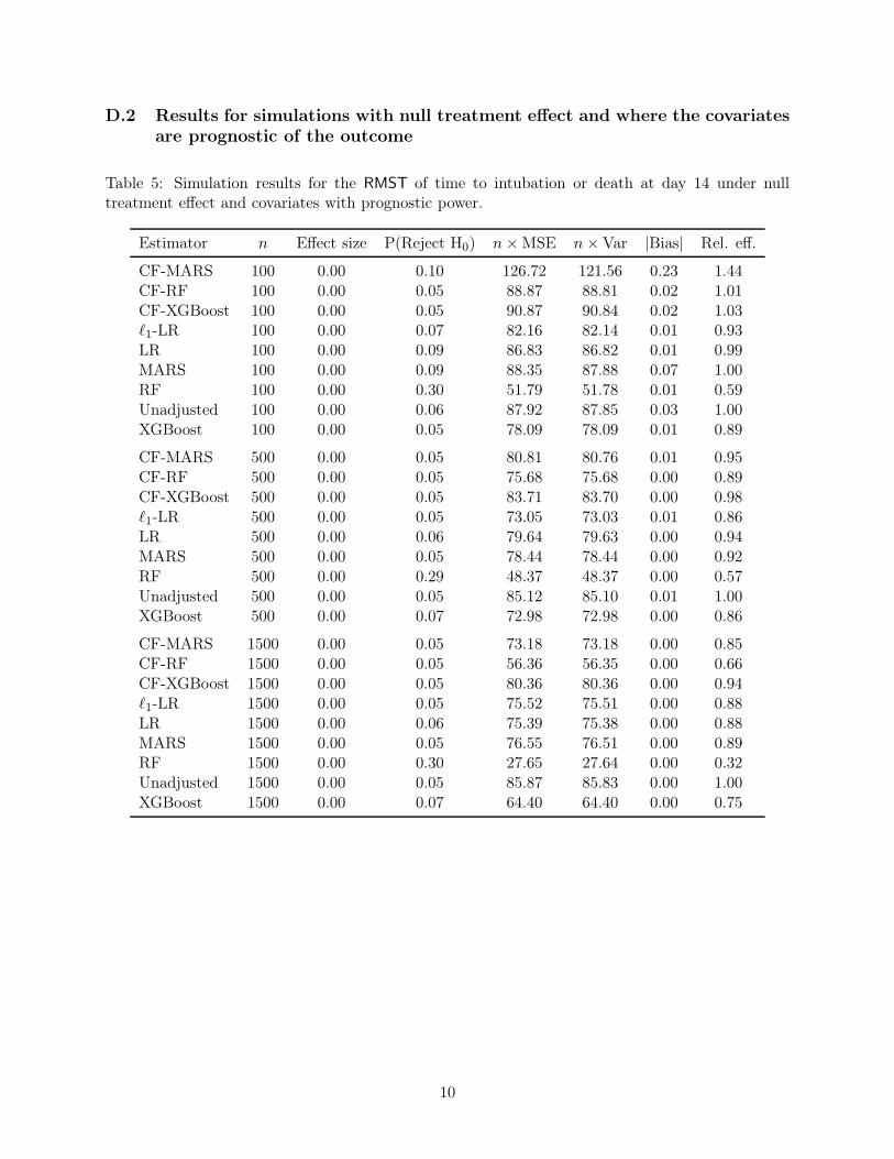
D.2 Results for simulations with null treatment effect and where the covariates
are prognostic of the outcome
Table 5: Simulation results for the RMST of time to intubation or death at day 14 under nulltreatment effect and covariates with prognostic power.
Estimator n Effect size P(Reject H0) n× MSE n× Var |Bias| Rel. eff.
CF-MARS 100 0.00 0.10 126.72 121.56 0.23 1.44CF-RF 100 0.00 0.05 88.87 88.81 0.02 1.01CF-XGBoost 100 0.00 0.05 90.87 90.84 0.02 1.03ℓ1-LR 100 0.00 0.07 82.16 82.14 0.01 0.93LR 100 0.00 0.09 86.83 86.82 0.01 0.99MARS 100 0.00 0.09 88.35 87.88 0.07 1.00RF 100 0.00 0.30 51.79 51.78 0.01 0.59Unadjusted 100 0.00 0.06 87.92 87.85 0.03 1.00XGBoost 100 0.00 0.05 78.09 78.09 0.01 0.89
CF-MARS 500 0.00 0.05 80.81 80.76 0.01 0.95CF-RF 500 0.00 0.05 75.68 75.68 0.00 0.89CF-XGBoost 500 0.00 0.05 83.71 83.70 0.00 0.98ℓ1-LR 500 0.00 0.05 73.05 73.03 0.01 0.86LR 500 0.00 0.06 79.64 79.63 0.00 0.94MARS 500 0.00 0.05 78.44 78.44 0.00 0.92RF 500 0.00 0.29 48.37 48.37 0.00 0.57Unadjusted 500 0.00 0.05 85.12 85.10 0.01 1.00XGBoost 500 0.00 0.07 72.98 72.98 0.00 0.86
CF-MARS 1500 0.00 0.05 73.18 73.18 0.00 0.85CF-RF 1500 0.00 0.05 56.36 56.35 0.00 0.66CF-XGBoost 1500 0.00 0.05 80.36 80.36 0.00 0.94ℓ1-LR 1500 0.00 0.05 75.52 75.51 0.00 0.88LR 1500 0.00 0.06 75.39 75.38 0.00 0.88MARS 1500 0.00 0.05 76.55 76.51 0.00 0.89RF 1500 0.00 0.30 27.65 27.64 0.00 0.32Unadjusted 1500 0.00 0.05 85.87 85.83 0.00 1.00XGBoost 1500 0.00 0.07 64.40 64.40 0.00 0.75
10

Table 6: Simulation results for the RD of time to intubation or death at day 7 under null treatmenteffect and covariates with prognostic power.
Estimator n Effect size P(Reject H0) n× MSE n× Var |Bias| Rel. eff.
CF-MARS 100 0.00 0.09 1.00 0.96 0.02 1.36CF-RF 100 0.00 0.05 0.75 0.75 0.00 1.02CF-XGBoost 100 0.00 0.05 0.75 0.75 0.00 1.03ℓ1-LR 100 0.00 0.07 0.69 0.69 0.00 0.95LR 100 0.00 0.09 0.72 0.72 0.00 0.98MARS 100 0.00 0.08 0.72 0.72 0.01 0.99RF 100 0.00 0.26 0.51 0.51 0.00 0.70Unadjusted 100 0.00 0.06 0.73 0.73 0.00 1.00XGBoost 100 0.00 0.05 0.66 0.66 0.00 0.90
CF-MARS 500 0.00 0.05 0.69 0.68 0.00 0.95CF-RF 500 0.00 0.04 0.63 0.63 0.00 0.88CF-XGBoost 500 0.00 0.04 0.70 0.70 0.00 0.98ℓ1-LR 500 0.00 0.05 0.63 0.63 0.00 0.88LR 500 0.00 0.06 0.69 0.69 0.00 0.95MARS 500 0.00 0.06 0.68 0.68 0.00 0.94RF 500 0.00 0.25 0.45 0.45 0.00 0.62Unadjusted 500 0.00 0.05 0.72 0.72 0.00 1.00XGBoost 500 0.00 0.06 0.62 0.62 0.00 0.86
CF-MARS 1500 0.00 0.04 0.62 0.62 0.00 0.86CF-RF 1500 0.00 0.05 0.49 0.49 0.00 0.67CF-XGBoost 1500 0.00 0.05 0.68 0.68 0.00 0.94ℓ1-LR 1500 0.00 0.05 0.64 0.64 0.00 0.89LR 1500 0.00 0.05 0.65 0.65 0.00 0.90MARS 1500 0.00 0.05 0.65 0.65 0.00 0.90RF 1500 0.00 0.25 0.26 0.26 0.00 0.36Unadjusted 1500 0.00 0.05 0.72 0.72 0.00 1.00XGBoost 1500 0.00 0.07 0.56 0.56 0.00 0.78
11

Table 7: Simulation results for the LOR of the modified WHO scale at day 14 under null treatmenteffect and covariates with prognostic power.
Estimator n Effect size P(Reject H0) n× MSE n× Var |Bias| Rel. eff.
CF-MARS 100 0.00 0.07 21.27 21.27 0.00 0.55CF-RF 100 0.00 0.06 16.93 16.93 0.01 0.44CF-XGBoost 100 0.00 0.07 18.12 18.12 0.00 0.47ℓ1-LR 100 0.00 0.09 28.01 28.01 0.00 0.73LR 100 0.00 0.11 111.68 111.61 0.03 2.89MARS 100 0.00 0.09 60.09 60.08 0.01 1.56RF 100 0.00 0.13 21.91 21.90 0.01 0.57Unadjusted 100 0.00 0.06 38.60 38.60 0.00 1.00XGBoost 100 0.00 0.10 18.97 18.96 0.01 0.49
CF-MARS 500 0.00 0.05 14.70 14.70 0.00 0.88CF-RF 500 0.00 0.05 12.57 12.57 0.00 0.75CF-XGBoost 500 0.00 0.06 14.07 14.06 0.00 0.84ℓ1-LR 500 0.00 0.06 13.51 13.51 0.00 0.81LR 500 0.00 0.06 13.76 13.75 0.00 0.82MARS 500 0.00 0.05 12.75 12.75 0.00 0.76RF 500 0.00 0.14 7.34 7.34 0.00 0.44Unadjusted 500 0.00 0.05 16.74 16.74 0.00 1.00XGBoost 500 0.00 0.08 11.07 11.07 0.00 0.66
CF-MARS 1500 0.00 0.05 13.35 13.35 0.00 0.82CF-RF 1500 0.00 0.05 8.36 8.36 0.00 0.51CF-XGBoost 1500 0.00 0.05 11.03 11.03 0.00 0.68ℓ1-LR 1500 0.00 0.05 12.87 12.87 0.00 0.79LR 1500 0.00 0.05 13.27 13.27 0.00 0.81MARS 1500 0.00 0.05 12.52 12.52 0.00 0.77RF 1500 0.00 0.15 4.56 4.56 0.00 0.28Unadjusted 1500 0.00 0.05 16.30 16.29 0.00 1.00XGBoost 1500 0.00 0.16 6.37 6.37 0.00 0.39
12

Table 8: Simulation results for the MW estimand of the modified WHO scale at day 14 under nulltreatment effect and covariates with prognostic power.
Estimator n Effect size P(Reject H0) n× MSE n× Var |Bias| Rel. eff.
CF-MARS 100 0.50 0.11 0.54 0.54 0.00 1.95CF-RF 100 0.50 0.07 0.23 0.23 0.00 0.84CF-XGBoost 100 0.50 0.07 0.25 0.25 0.00 0.92ℓ1-LR 100 0.50 0.07 0.22 0.22 0.00 0.80LR 100 0.50 0.48 2.14 2.14 0.00 7.77MARS 100 0.50 0.12 0.43 0.43 0.00 1.58RF 100 0.50 0.13 0.16 0.16 0.00 0.57Unadjusted 100 0.50 0.06 0.28 0.28 0.00 1.00XGBoost 100 0.50 0.09 0.21 0.21 0.00 0.75
CF-MARS 500 0.50 0.06 0.28 0.28 0.00 1.07CF-RF 500 0.50 0.05 0.20 0.20 0.00 0.74CF-XGBoost 500 0.50 0.06 0.22 0.22 0.00 0.85ℓ1-LR 500 0.50 0.05 0.21 0.21 0.00 0.80LR 500 0.50 0.08 0.79 0.79 0.00 2.98MARS 500 0.50 0.06 0.27 0.27 0.00 1.01RF 500 0.50 0.14 0.13 0.13 0.00 0.48Unadjusted 500 0.50 0.05 0.27 0.27 0.00 1.00XGBoost 500 0.50 0.08 0.18 0.18 0.00 0.69
CF-MARS 1500 0.50 0.05 0.22 0.22 0.00 0.84CF-RF 1500 0.50 0.05 0.13 0.13 0.00 0.52CF-XGBoost 1500 0.50 0.06 0.18 0.18 0.00 0.71ℓ1-LR 1500 0.50 0.05 0.21 0.21 0.00 0.81LR 1500 0.50 0.06 0.22 0.22 0.00 0.84MARS 1500 0.50 0.05 0.22 0.22 0.00 0.84RF 1500 0.50 0.16 0.20 0.20 0.00 0.78Unadjusted 1500 0.50 0.05 0.26 0.26 0.00 1.00XGBoost 1500 0.50 0.15 0.11 0.11 0.00 0.43
13

D.3 Results for simulations with a positive effect and where the covariates are
not prognostic of the outcome
Table 9: Simulation results for the RMST of the time to intubation or death at day 14 under apositive effect and covariates with no prognostic power.
Estimator n Effect size P(Reject H0) n× MSE n× Var |Bias| Rel. eff.
CF-MARS 100 1.04 0.25 94.58 94.56 0.01 1.46CF-RF 100 1.04 0.21 77.13 77.13 0.00 1.19CF-XGBoost 100 1.04 0.23 77.43 77.41 0.01 1.20ℓ1-LR 100 1.04 0.24 64.21 64.21 0.01 0.99LR 100 1.04 0.30 75.60 75.55 0.02 1.17MARS 100 1.04 0.25 73.38 72.61 0.09 1.14RF 100 1.04 0.58 68.20 64.12 0.20 1.06Unadjusted 100 1.04 0.25 64.64 64.64 0.01 1.00XGBoost 100 1.04 0.26 66.74 66.74 0.01 1.03
CF-MARS 500 1.04 0.81 67.36 67.36 0.00 1.02CF-RF 500 1.04 0.77 74.08 74.06 0.01 1.12CF-XGBoost 500 1.04 0.77 73.22 73.21 0.00 1.11ℓ1-LR 500 1.04 0.83 66.61 66.61 0.00 1.01LR 500 1.04 0.83 68.06 68.04 0.01 1.03MARS 500 1.04 0.82 64.56 64.54 0.01 0.98RF 500 1.04 0.91 81.56 79.70 0.06 1.24Unadjusted 500 1.04 0.82 65.85 65.85 0.00 1.00XGBoost 500 1.04 0.83 63.75 63.70 0.01 0.97
CF-MARS 1500 1.04 1.00 65.62 65.61 0.00 1.01CF-RF 1500 1.04 1.00 73.92 73.91 0.00 1.14CF-XGBoost 1500 1.04 1.00 70.56 70.55 0.00 1.08ℓ1-LR 1500 1.04 1.00 65.55 65.54 0.00 1.01LR 1500 1.04 1.00 65.55 65.55 0.00 1.01MARS 1500 1.04 1.00 65.68 65.67 0.00 1.01RF 1500 1.04 1.00 74.73 74.72 0.00 1.15Unadjusted 1500 1.04 1.00 65.07 65.06 0.00 1.00XGBoost 1500 1.04 1.00 66.71 66.69 0.00 1.03
14

Table 10: Simulation results for the RD of the time to intubation or death at day 7 under a positiveeffect and covariates with no prognostic power.
Estimator n Effect size P(Reject H0) n× MSE n× Var |Bias| Rel. eff.
CF-MARS 100 0.10 0.26 0.83 0.83 0.00 1.39CF-RF 100 0.10 0.22 0.68 0.68 0.00 1.14CF-XGBoost 100 0.10 0.26 0.70 0.70 0.00 1.17ℓ1-LR 100 0.10 0.26 0.60 0.60 0.00 1.00LR 100 0.10 0.30 0.67 0.67 0.00 1.13MARS 100 0.10 0.27 0.67 0.67 0.01 1.13RF 100 0.10 0.51 0.71 0.68 0.02 1.18Unadjusted 100 0.10 0.26 0.60 0.60 0.00 1.00XGBoost 100 0.10 0.27 0.62 0.62 0.00 1.03
CF-MARS 500 0.10 0.82 0.61 0.61 0.00 1.00CF-RF 500 0.10 0.79 0.66 0.66 0.00 1.08CF-XGBoost 500 0.10 0.79 0.66 0.66 0.00 1.07ℓ1-LR 500 0.10 0.83 0.61 0.61 0.00 0.99LR 500 0.10 0.83 0.62 0.62 0.00 1.02MARS 500 0.10 0.83 0.59 0.59 0.00 0.96RF 500 0.10 0.89 0.79 0.77 0.01 1.28Unadjusted 500 0.10 0.83 0.61 0.61 0.00 1.00XGBoost 500 0.10 0.83 0.60 0.59 0.00 0.97
CF-MARS 1500 0.10 1.00 0.61 0.61 0.00 1.01CF-RF 1500 0.10 1.00 0.67 0.67 0.00 1.11CF-XGBoost 1500 0.10 1.00 0.63 0.63 0.00 1.05ℓ1-LR 1500 0.10 1.00 0.60 0.60 0.00 0.99LR 1500 0.10 1.00 0.60 0.60 0.00 0.99MARS 1500 0.10 1.00 0.60 0.60 0.00 0.99RF 1500 0.10 1.00 0.69 0.69 0.00 1.14Unadjusted 1500 0.10 1.00 0.60 0.60 0.00 1.00XGBoost 1500 0.10 1.00 0.61 0.61 0.00 1.01
15

Table 11: Simulation results for the LOR of the modified WHO scale at day 14 under a positiveeffect and covariates with no prognostic power.
Estimator n Effect size P(Reject H0) n× MSE n× Var |Bias| Rel. eff.
CF-MARS 100 0.60 0.35 67.15 64.59 0.16 0.12CF-RF 100 0.60 0.37 62.46 58.98 0.19 0.11CF-XGBoost 100 0.60 0.40 76.06 72.37 0.19 0.13ℓ1-LR 100 0.60 0.44 95.99 90.49 0.23 0.16LR 100 0.60 0.41 392.58 330.71 0.79 0.67MARS 100 0.60 0.41 187.85 167.51 0.45 0.32RF 100 0.60 0.45 61.04 59.51 0.12 0.10Unadjusted 100 0.60 0.42 582.27 441.29 1.19 1.00XGBoost 100 0.60 0.43 132.91 124.69 0.29 0.23
CF-MARS 500 0.60 0.87 31.28 31.16 0.02 0.56CF-RF 500 0.60 0.87 23.06 23.05 0.00 0.41CF-XGBoost 500 0.60 0.88 25.83 25.62 0.02 0.46ℓ1-LR 500 0.60 0.87 24.01 23.98 0.01 0.43LR 500 0.60 0.86 53.78 53.45 0.03 0.96MARS 500 0.60 0.87 39.20 39.04 0.02 0.70RF 500 0.60 0.91 33.77 33.77 0.00 0.60Unadjusted 500 0.60 0.86 56.01 55.76 0.02 1.00XGBoost 500 0.60 0.89 22.54 22.54 0.00 0.40
CF-MARS 1500 0.60 1.00 20.98 20.98 0.00 1.04CF-RF 1500 0.60 1.00 20.93 20.92 0.00 1.04CF-XGBoost 1500 0.60 1.00 22.14 22.09 0.01 1.10ℓ1-LR 1500 0.60 1.00 20.81 20.80 0.00 1.03LR 1500 0.60 1.00 20.27 20.26 0.00 1.00MARS 1500 0.60 1.00 20.16 20.15 0.00 1.00RF 1500 0.60 1.00 20.51 20.48 0.00 1.02Unadjusted 1500 0.60 1.00 20.20 20.20 0.00 1.00XGBoost 1500 0.60 1.00 20.48 20.44 0.01 1.01
16

Table 12: Simulation results for the MW of the modified WHO scale at day 14 under a positiveeffect and covariates with no prognostic power.
Estimator n Effect size P(Reject H0) n× MSE n× Var |Bias| Rel. eff.
CF-MARS 100 0.46 0.18 0.54 0.54 0.00 2.05CF-RF 100 0.46 0.15 0.29 0.29 0.00 1.11CF-XGBoost 100 0.46 0.15 0.29 0.29 0.00 1.10ℓ1-LR 100 0.46 0.16 0.26 0.26 0.00 1.00LR 100 0.46 0.44 1.69 1.67 0.01 6.43MARS 100 0.46 0.18 0.43 0.43 0.00 1.63RF 100 0.46 0.19 0.24 0.23 0.01 0.91Unadjusted 100 0.46 0.14 0.26 0.26 0.00 1.00XGBoost 100 0.46 0.18 0.26 0.26 0.00 1.00
CF-MARS 500 0.46 0.44 0.50 0.49 0.00 1.93CF-RF 500 0.46 0.44 0.28 0.28 0.00 1.09CF-XGBoost 500 0.46 0.46 0.27 0.27 0.00 1.04ℓ1-LR 500 0.46 0.46 0.26 0.26 0.00 1.02LR 500 0.46 0.46 0.29 0.28 0.00 1.10MARS 500 0.46 0.44 0.30 0.30 0.00 1.16RF 500 0.46 0.51 0.24 0.24 0.00 0.93Unadjusted 500 0.46 0.44 0.26 0.26 0.00 1.00XGBoost 500 0.46 0.47 0.26 0.25 0.00 0.98
CF-MARS 1500 0.46 0.87 0.28 0.27 0.00 1.04CF-RF 1500 0.46 0.88 0.27 0.27 0.00 1.03CF-XGBoost 1500 0.46 0.88 0.28 0.27 0.00 1.06ℓ1-LR 1500 0.46 0.88 0.27 0.26 0.00 1.00LR 1500 0.46 0.89 0.26 0.25 0.00 0.98MARS 1500 0.46 0.88 0.27 0.26 0.00 1.03RF 1500 0.46 0.91 0.26 0.26 0.00 0.98Unadjusted 1500 0.46 0.88 0.27 0.26 0.00 1.00XGBoost 1500 0.46 0.89 0.27 0.26 0.00 1.01
17

D.4 Results for simulations with null treatment effect and where the covariates
are not prognostic of the outcome
Table 13: Simulation results for the RMST of the time to intubation or death at day 14 under nulltreatment effect and covariates with no prognostic power.
Estimator n Effect size P(Reject H0) n× MSE n× Var |Bias| Rel. eff.
CF-MARS 100 0.00 0.11 142.00 135.82 0.25 1.62CF-RF 100 0.00 0.05 103.14 103.11 0.02 1.17CF-XGBoost 100 0.00 0.05 95.76 95.76 0.00 1.09ℓ1-LR 100 0.00 0.06 87.21 87.13 0.03 0.99LR 100 0.00 0.09 99.98 99.95 0.02 1.14MARS 100 0.00 0.08 97.67 97.24 0.07 1.11RF 100 0.00 0.31 70.72 70.68 0.02 0.80Unadjusted 100 0.00 0.06 87.92 87.85 0.03 1.00XGBoost 100 0.00 0.06 87.83 87.82 0.01 1.00
CF-MARS 500 0.00 0.06 91.82 91.53 0.02 1.08CF-RF 500 0.00 0.05 98.39 98.38 0.00 1.16CF-XGBoost 500 0.00 0.05 97.91 97.91 0.00 1.15ℓ1-LR 500 0.00 0.05 87.33 87.32 0.01 1.03LR 500 0.00 0.06 92.74 92.74 0.00 1.09MARS 500 0.00 0.05 88.10 88.10 0.00 1.04RF 500 0.00 0.17 86.34 86.34 0.00 1.01Unadjusted 500 0.00 0.05 85.12 85.10 0.01 1.00XGBoost 500 0.00 0.06 86.89 86.89 0.00 1.02
CF-MARS 1500 0.00 0.05 85.92 85.89 0.00 1.00CF-RF 1500 0.00 0.05 94.58 94.57 0.00 1.10CF-XGBoost 1500 0.00 0.04 93.27 93.26 0.00 1.09ℓ1-LR 1500 0.00 0.05 85.62 85.61 0.00 1.00LR 1500 0.00 0.06 90.04 90.01 0.00 1.05MARS 1500 0.00 0.05 89.32 89.32 0.00 1.04RF 1500 0.00 0.11 89.12 89.12 0.00 1.04Unadjusted 1500 0.00 0.05 85.87 85.83 0.00 1.00XGBoost 1500 0.00 0.07 89.61 89.59 0.00 1.04
18

Table 14: Simulation results for the RD of the time to intubation or death at day 7 under nulltreatment effect and covariates with no prognostic power.
Estimator n Effect size P(Reject H0) n× MSE n× Var |Bias| Rel. eff.
CF-MARS 100 0.00 0.10 1.11 1.07 0.02 1.52CF-RF 100 0.00 0.05 0.85 0.85 0.00 1.17CF-XGBoost 100 0.00 0.05 0.80 0.80 0.00 1.09ℓ1-LR 100 0.00 0.06 0.72 0.72 0.00 0.99LR 100 0.00 0.08 0.82 0.82 0.00 1.12MARS 100 0.00 0.07 0.79 0.79 0.00 1.09RF 100 0.00 0.27 0.66 0.66 0.00 0.90Unadjusted 100 0.00 0.06 0.73 0.73 0.00 1.00XGBoost 100 0.00 0.06 0.73 0.73 0.00 1.00
CF-MARS 500 0.00 0.05 0.76 0.76 0.00 1.06CF-RF 500 0.00 0.05 0.82 0.82 0.00 1.13CF-XGBoost 500 0.00 0.05 0.80 0.80 0.00 1.11ℓ1-LR 500 0.00 0.05 0.72 0.72 0.00 1.00LR 500 0.00 0.06 0.78 0.78 0.00 1.08MARS 500 0.00 0.05 0.74 0.74 0.00 1.03RF 500 0.00 0.16 0.73 0.73 0.00 1.02Unadjusted 500 0.00 0.05 0.72 0.72 0.00 1.00XGBoost 500 0.00 0.06 0.72 0.72 0.00 1.00
CF-MARS 1500 0.00 0.05 0.71 0.71 0.00 0.99CF-RF 1500 0.00 0.05 0.79 0.79 0.00 1.09CF-XGBoost 1500 0.00 0.04 0.77 0.77 0.00 1.07ℓ1-LR 1500 0.00 0.05 0.72 0.72 0.00 0.99LR 1500 0.00 0.06 0.74 0.74 0.00 1.03MARS 1500 0.00 0.05 0.74 0.74 0.00 1.03RF 1500 0.00 0.10 0.74 0.74 0.00 1.03Unadjusted 1500 0.00 0.05 0.72 0.72 0.00 1.00XGBoost 1500 0.00 0.06 0.75 0.75 0.00 1.05
19

Table 15: Simulation results for the LOR of the modified WHO scale at day 14 under null treatmenteffect and covariates with no prognostic power.
Estimator n Effect size P(Reject H0) n× MSE n× Var |Bias| Rel. eff.
CF-MARS 100 0.00 0.07 38.32 38.30 0.01 0.99CF-RF 100 0.00 0.06 20.08 20.07 0.01 0.52CF-XGBoost 100 0.00 0.07 21.21 21.21 0.00 0.55ℓ1-LR 100 0.00 0.09 22.15 22.15 0.01 0.57LR 100 0.00 0.08 96.02 96.02 0.00 2.49MARS 100 0.00 0.07 28.91 28.90 0.01 0.75RF 100 0.00 0.11 16.61 16.60 0.01 0.43Unadjusted 100 0.00 0.06 38.60 38.60 0.00 1.00XGBoost 100 0.00 0.10 34.50 34.48 0.01 0.89
CF-MARS 500 0.00 0.05 16.92 16.91 0.00 1.01CF-RF 500 0.00 0.05 17.27 17.27 0.00 1.03CF-XGBoost 500 0.00 0.06 17.75 17.74 0.00 1.06ℓ1-LR 500 0.00 0.06 16.45 16.45 0.00 0.98LR 500 0.00 0.06 17.28 17.28 0.00 1.03MARS 500 0.00 0.06 17.26 17.26 0.00 1.03RF 500 0.00 0.09 15.20 15.20 0.00 0.91Unadjusted 500 0.00 0.05 16.74 16.74 0.00 1.00XGBoost 500 0.00 0.07 16.54 16.54 0.00 0.99
CF-MARS 1500 0.00 0.05 16.60 16.60 0.00 1.02CF-RF 1500 0.00 0.06 17.37 17.37 0.00 1.07CF-XGBoost 1500 0.00 0.06 17.11 17.11 0.00 1.05ℓ1-LR 1500 0.00 0.05 16.33 16.28 0.01 1.00LR 1500 0.00 0.05 16.61 16.61 0.00 1.02MARS 1500 0.00 0.05 16.25 16.24 0.00 1.00RF 1500 0.00 0.08 16.21 16.21 0.00 0.99Unadjusted 1500 0.00 0.05 16.30 16.29 0.00 1.00XGBoost 1500 0.00 0.06 16.30 16.29 0.00 1.00
20

Table 16: Simulation results for the MW of the modified WHO scale at day 14 under null treatmenteffect and covariates with no prognostic power.
Estimator n Effect size P(Reject H0) n× MSE n× Var |Bias| Rel. eff.
CF-MARS 100 0.50 0.08 0.42 0.42 0.00 1.54CF-RF 100 0.50 0.06 0.28 0.28 0.00 1.02CF-XGBoost 100 0.50 0.07 0.29 0.29 0.00 1.07ℓ1-LR 100 0.50 0.07 0.27 0.27 0.00 0.99LR 100 0.50 0.47 2.09 2.09 0.00 7.57MARS 100 0.50 0.08 0.36 0.36 0.00 1.32RF 100 0.50 0.11 0.22 0.22 0.00 0.79Unadjusted 100 0.50 0.06 0.28 0.28 0.00 1.00XGBoost 100 0.50 0.09 0.27 0.27 0.00 0.97
CF-MARS 500 0.50 0.05 0.28 0.28 0.00 1.04CF-RF 500 0.50 0.06 0.28 0.28 0.00 1.04CF-XGBoost 500 0.50 0.06 0.29 0.29 0.00 1.07ℓ1-LR 500 0.50 0.05 0.26 0.26 0.00 0.99LR 500 0.50 0.08 0.72 0.72 0.00 2.69MARS 500 0.50 0.06 0.28 0.28 0.00 1.05RF 500 0.50 0.09 0.24 0.24 0.00 0.91Unadjusted 500 0.50 0.05 0.27 0.27 0.00 1.00XGBoost 500 0.50 0.07 0.26 0.26 0.00 0.99
CF-MARS 1500 0.50 0.05 0.27 0.27 0.00 1.03CF-RF 1500 0.50 0.06 0.28 0.28 0.00 1.08CF-XGBoost 1500 0.50 0.06 0.28 0.28 0.00 1.06ℓ1-LR 1500 0.50 0.05 0.26 0.26 0.00 1.02LR 1500 0.50 0.05 0.27 0.27 0.00 1.03MARS 1500 0.50 0.05 0.26 0.26 0.00 1.00RF 1500 0.50 0.08 0.26 0.26 0.00 1.00Unadjusted 1500 0.50 0.05 0.26 0.26 0.00 1.00XGBoost 1500 0.50 0.06 0.27 0.27 0.00 1.02
References
P.J. Bickel, C.A.J. Klaassen, Y. Ritov, and J. Wellner. Efficient and Adaptive Estimation for
Semiparametric Models. Springer-Verlag, 1997.
Iván Díaz, Oleksandr Savenkov, and Karla Ballman. Targeted learning ensembles for optimalindividualized treatment rules with time-to-event outcomes. Biometrika, 105(3):723–738, 2018.
Iván Díaz, Elizabeth Colantuoni, Daniel F. Hanley, and Michael Rosenblum. Improved precision inthe analysis of randomized trials with survival outcomes, without assuming proportional hazards.Lifetime Data Analysis, 25(3):439–468, 2019.
Kelly L. Moore and Mark J. van der Laan. Increasing power in randomized trials with rightcensored outcomes through covariate adjustment. Journal of Biopharmaceutical Statistics, 19(6):1099–1131, 2009.
21

A. W. van der Vaart. Asymptotic Statistics. Cambridge University Press, 1998.
Aad W. van der Vaart and Jon A. Wellner. Weak Convergence and Emprical Processes. Springer-Verlag New York, 1996.
22