Optimum Liquidation Problem Associated with

the Poisson Cluster Process

Amirhossein Sadoghi 1 , Jan Vecer

Frankfurt School of Finance & Management, Frankfurt am Main

Abstract

In this research, we develop a trading strategy for the discrete-time optimalliquidation problem of large order trading with different market microstruc-tures in an illiquid market. In this framework, the flow of orders can beviewed as a point process with stochastic intensity. We model the price im-pact as a linear function of a self-exciting dynamic process. We formulatethe liquidation problem as a discrete-time Markov Decision Processes, wherethe state process is a Piecewise Deterministic Markov Process (PDMP). Thenumerical results indicate that an optimal trading strategy is dependent oncharacteristics of the market microstructure. When no orders above certainvalue come the optimal solution takes offers in the lower levels of the limitorder book in order to prevent not filling of orders and facing final inventorycosts.

Keywords: Optimum Liquidation Problem, Discrete order books,Markov-modulated Poisson process, PDMP, Hawkes processes

1Corresponding Author, address: Sonnemannstrae 9-11 60314 Frankfurt am Main,Tel: +49(069)154008-873. We are grateful for the comments of participants of FirstBerlin-Singapore Workshop on Quantitative Finance & Financial Risk, Berlin, 2014.Bachelier Finance Society 8th World Congress Brussels, 2014. SIAM Conference onFinancial Mathematics & Engineering, Chicago, 2014. 38th conference StochasticProcesses & their Applications, 2015, Oxford.

JEL classification: C60, C61, D4, G1.Email addresses: a.sadoghi@fs.de (Amirhossein Sadoghi ), j.vecer@fs.de (Jan

Vecer)

Preprint submitted to Journal October 16, 2018

arX

iv:1

507.

0651

4v2

[q-

fin.

TR

] 2

5 D

ec 2

015

1. Introduction

In an illiquid market, due to lack of counterparties and uncertainty aboutthe assets’ value, trading of assets by fair value is not guaranteed. In amarket like this, a trader faces liquidity restrictions, and behaves differentlyin comparison to an unconstrained market. Depending on the elasticity ofthe market, the effect of an increased offer will be compensated by a dropin prices. Effectively, the initial price impact partially is temporary, andvanishes after the execution of the order depending on the elasticity of themarket. Early liquidation causes an unfavorable influence on the stock price,and a late execution has liquidity risk since the stock price can move awayfrom that at the beginning of the period.

Most practitioners deal with this dilemma by predicting the trend of stockprice and adjusting their order execution speed. While the stock price startsto go down, they send positive signals to market by decreasing rapidly thesize of order; otherwise, they should wait until the end of execution periodwhen the position becomes urgent to liquidate. In such a situation, whenthey expect the stock price starts to rise, they split orders and execute withoffers in deeper levels in the order book to gain an advantage from increas-ing stock prices. Liquidation of large block orders has an impact on marketresilience and market depth. Lack of transparency in a market and splittingtrade share help larger traders to avoid reorganization by other participants,who can move against them.

In this research, we determine the optimal liquidation strategy of a singletrader, who wants to liquidate a large portfolio in an illiquid market. Weformulate the liquidation problem as a multi-stopping problem with Poissonarrival patterns of order in a discrete-time model. We set up a stochasticcontrol framework to maximize the expected revenue of trading in the entireexecution time taking into consideration the liquidity restriction of trading alarge order. The assumption of the discrete-time framework is not far fromthe classical trading algorithms. In most continuous liquidation problemsetups, it is assumed that supply and demand are in balance; this is onlypossible in a liquid market. We show how the current state of the arrivalrates of limit orders in the order book can be used to compute price impactin terms of the conditional distribution of price changes.

2

The optimal liquidation problem can be defined as an optimal controlproblem to determine optimal strategies for trading stock portfolios by min-imizing the entire cost function. These strategies depend on the state of themarket as well as price and size of stocks available during the execution ofthe limit orders. To find an optimal solution, we need to consider a trade-offbetween liquidity risk and changing the stock price. The former resultingin in slow order execution and latter caused by exogenous events or a rapidliquidation. Optimal liquidation problems seeks optimal strategies for trad-ing stock with regards to both liquidity risks and non-execution risks. Theserisks are attributable to liquidity restrictions and time delay of executionorders.

The study of the optimal execution problem dates back to 1990’s, andmainly focuses on the discrete-time models that optimal strategies are deter-mined as optimal liquidation rates per unit time. Bertsimas and Lo (1998)studied the optimal liquidation of a large block of shares with linear per-manent price impact in a fixed time horizon. Almgren and Chriss (2001)as one of the most cited optimal execution models, used a diffusion priceprocess in a continuous-time trading space. They constructed an efficientfrontier of execution strategies via mean-variance analysis of expected costsof liquidation and divided the price impact into temporary and/or linear per-manent impact. From a traditional view point on this problem (e.g. (Alfonsiand Schied, 2010), and (Alfonsi et al., 2010)), the optimal liquidation de-pends on existence of a sufficiently large limit order in the limit order book,and price impact is a function of the shape and depth of the limit order book.

Bayraktar and Ludkovski (2014) formulated the liquidation problem asa Hamilton–Jacobi–Bellman equation association with the depth function ofthe limit order book. A recent study by Horst and Naujokat (2014) addressedthe problem of optimal trading in illiquid markets. They studied a tradingalgorithm with a two-sided limit order market as well as market orders ina dark pool by controlling the bid-ask spread. Their algorithm determinedthe optimal time of crossing the bid-ask spread which is a primary problemof algorithmic trading. Under the same market condition, Horst and Nau-jokat (2011) studied optimal trading problems in an option market. In theirmathematical framework, risk-neutral and risk averse investors hold Euro-pean contingent claims and the price evolution of the underlying is affectedby agents’ trading. They proved the existence and uniqueness of equilibrium

3

for a number of interacting players of the market.

An optimal stopping problem is a link between the control theory andmarket microstructure. This problem has been studied as a single or multi-stopping problem in the classical house selling problems or best choice prob-lems by using homogeneous Poisson processes. Single stopping time problemgoverned with Poisson Process was formulated as a best choice problem in thelate 1950’s by Lindley (1961). The optimal k-stopping problem with finiteand infinite time horizon was presented with the complete solution by Peskirand Shiryaev (2006) in a Bayesian formulation. A similar problem, which hasbeen considered in the market microstructure literature by (Garman, 1976),studied a trading problem of a market maker who maximizes her profit byassuming order arrival rates depending on the price dynamics governed bythe Poisson process. Smith et al. (2003) simulated the buy and sell orderwith thr Poisson process in which the arrival rates are independent of thestate of the order book. Recent study by (Cont et al., 2010) used Laplacetransforms to analyze the behavior of the order-book with Poisson arrivalsof buy and sell orders.

The homogeneous Poisson Process of sell and buy orders arrival rate wasthe main assumption of past studies. Garman (1976) explained conditionsnecessary and sufficient for the order arrival patterns to be modeled by a ho-mogeneous Poisson processor. In this framework, none of the agents’ tradingcan dominate other agents or they place a large number of limit orders ina finite time. Nevertheless, most of these assumptions are violated in thehigh-frequency trading. Empirical studies of high-frequency data show thatthere are significant cross-correlation patterns of the arrival rate of similarlimit buy or sell orders and significant autocorrelation in durations of events,(see: Cont (2011)).

Some empirical studies like Bacry et al. (2013) showed that high frequencydata can be modeled by Hawkes processes, introduced by HAWKES (1971).The irregularity properties of high frequency financial data can be explainedby self-exciting and mutually-exciting properties of the Hawkes processes.Engle and Lunde (2003) modeled trade and quote arrivals with bivariatepoint processes.

In the illiquid market, the disparity between supply and demand causes

4

illiquidity, which means the executing larger positions need longer time. Weformulate the liquidation problem as a discrete-time Markov Decision Pro-cesses (MDP) where the state process is a Piecewise Deterministic MarkovProcess (PDMP), which is a member of right continuous Markov Processfamily introduced by Davis (1984). By applying a MDP approach, we decom-pose the liquidation problem as a continuous-time stochastic control probleminto multiplies deterministic optimal control problems and construct an ap-proximation of value function with a quantization method proposed by Ballyet al. (2003). In our numerical simulation, we compare the performance ofour algorithm with regard to various market characteristics and price impactfunctions.

The numerical results show that the trading strategy is dependent on thecharacteristics of market microstructure and dynamics of incoming orders. Inthe case of favorite offers are not coming, our algorithm will reduce the speedof trading and allows the trader to go deeper into limit order book to avoidnot filling of orders and facing an ultimate inventory penalty. The simulatedresults indicate that higher probability of same types of orders’ occurrences(self-exciting property of the point process), creates more profitable tradingopportunities.

The remainder of this paper is organized as follows. Section 2 describesthe statistical model of order book. Section 3 explains the market modelsetup and present the problem statement. Section 4 presents the stochasticdynamic of the intensity of the order arrival process. In section 5, we turnto model price impact. Section 6 describes the procedure of solution withusing discrete-time Markov Process. In section 7, we explain the numericalmethod for optimal stopping time and simulate with different micromarketstructures. Section 8 summarizes the results, and concludes the paper withfurther remarks.

2. Statistics Model of Limit Order Book

To understand the behavior of market participants, we need to analyzethe stochastic fluctuation of stock price and the reaction of players in themarket. These fluctuations can be explained by a sequence of equilibria ofdemand and supply in the market. In order-driven markets, buy and sell or-ders arrive at different time points and wait in the LOB (Limit Order Book)

5

to be traded. The limit order book contains information about orders likequantity, price and type of orders. This information can be used to reducethe complexity of the relation between price fluctuations and limit order bookdynamic. It also help to predict different market’s quantities conditional onthe current state of the order book. On other hand, this Information mightbe used against counter-parties to take advantage of price movement. Theidea of the dark pool to reduce the information linkage and adverse price risk.

Cont et al. (2010) shows that this information contains short-term pricemovements and might change quickly during the trading period. In illiquidmarkets, the relation between limit order book dynamics and the price be-havior shows that the less liquid assets wait for a longer time to be executed.Therefore queue type models can be applied to analyze the orders arrivalin the limit order book. Cont et al. (2010) developed a tractable stochasticmodel of limit order markets to capture the main statistical features of limitorder books.

The statistical characteristics of the limit order book are well-documentedby Smith et al. (2003). Garman (1976), Bayraktar et al. (2007) studied thefluctuation of the orders arrival in the electronic trading market. Some stud-ies explained the unconditional and steady-state distributions of the orderbook while Cont et al. (2010) showed the short-term price movements couldbe explained by the information on the current state of the limit order book.Their model is based on the dynamics of the best bid and offer queues sincethe best orders can move the price.

Underlying our approach is that the dynamics of limit orders arrivals fol-low a Poisson pattern of prices depending on rates of trading. We study thestochastic dynamics of the arrival rate of limit order with the help of orderstatistics.

Distribution of a limit order book

We assume in a financial market, the price processes (Sjt )(j=1···d) of limitorders satisfy the following stochastic dynamic in a finite discrete-time hori-zon t ∈ τ = 1 < T1 · · · < Tm < n:

Sjt = Sj0(µjdt+ dCjt ), (2.1)

6

where Ct =∑Nt

n=1 Jn, and Jn is an independent and identically distributedrandom variable and Nt counting process.Given a vector of price of buy (sell) orders (Sjt )1≤j≤d on the probability space

(Ω;F ;P), the orders are sorted into a vector (S(1)t , S

(2)t , · · · , S(j)

t ) satisfy:

(S(1)t ≤ S

(2)t , · · · ,≤ S

(j)t )

The vector (S(1)t , S

(2)t , · · · , S(j)

t ) is a so-called vector of order statistics of theprice processes (Sjt ).

Let L be the number of unexecuted orders at the time point s. In thetime interval (s, t), the rate of arrival of limit orders is governed by a Poissonprocess. It is assumed that noisy traders cannot have a strong influence onthe market, and no cancellation or strategic cancellation of orders can occur.Hence, this model is a pure birth Poisson process with intensity λ, and thearrivals of orders in the non-overlapping intervals are independent.

In a small time interval dt , the probability that a limit order arrives andsits in the limit order book is:

P (N(dt) = 1) = λdt1!e−λdt = λdt+O(dt)

Similarly, the probability that no limit order appears in the limit order bookin this interval is:

P (N(dt) = 0) = e−λdt = 1− λdt+O(dt)

Figure 1: Orders’ arrival governed by Poisson process

Theorem 1 (Distribution of the limit order book). Denote by L thenumber of unexecuted orders at time s. We assume that in the interval (0, t),the number of orders (Nt) is a random variable with the Poisson distribution

7

with mean value λt. Vector S1t , · · · , SNtt represents the prices of buy (sell)

orders with distribution F (S) on the probability space (Ω;F ;P). U is thenumber of unexecuted orders with prices greater than Y = maxS1

t , · · · , SNtt ,then the probability of having k unexecuted orders with prices greater than Yis:

P (U = k|Ns = L) =e−λY · λkY

k!,

where

λY = λ[1− F (Y )t− ln(eλF (Y ) − λL+1

(L+ 1)!)].

(Proof is given in the appendix)With given k = 0 , equation 2.2 gives the probability of best orders (i.e. noneof orders with price (Sit)i∈1,···,Nt has greater price than Y ), with k = 1 givesthe probability of the second best order,and so on.

3. Market Model Setup

It is assumed that our financial market consists of an illiquid asset, itcan be considered as a risky asset, and a risk-free asset as a numeraire withthe interest rate r. The market for the risk-free asset is liquid, that meanstraders can liquidate a large amount of this security without facing costs ofprice impact.

In a complete financial market with a finite discrete-time horizon τ =1 < T1 · · · < Tm < n, the price process St is a stochastic process on a com-plete filtered probability space (Ω;F ;F;P) where F is the filtration generatedby Ftt∈τ . This space is bounded by a maturity time T .

The assumption of the finite discrete-time space is contradiction to con-ventional liquidation problems. However, it is not far away from reality;order arrival patterns of buy and sell orders are not the same. Because of thefluctuation in the stock market, especially in a high-frequency environment,orders might not appear regularly in the LOB. Some empirical studies showthat in a short period of time, the percentage changes of the stock price are

8

not uniformly distributed with same centrality, but price process can be in-ternally steady state processes. Therefore, the model should be solved andinterpreted in the discrete time and space. We use these facts and propose amodel with the rate of incoming buy orders as a Poisson process in a finitediscrete-time and space.

3.1. Trading Boundaries

Traders often follow trends of the prices and construct trading bound-aries built in on market depth. They submit limit orders at touch with anoptimum volume when the stock prices hit one of these trading boundaries.Market depth reflects the information related to the prices of buy and sellorders for the price and depends on trade volume, and minimum price incre-ment known as tick size. It is constantly changing, and reflects the valuableinformation about the current orders sitting in the limit order book. Know-ing this information helps traders to understand hidden patterns of pricemovements and price impact. Traders can use this potential information,and regulate their orders in response to the net order flow.

Cont et al. (2014) studied the link between price impact and market depthand showed that there is a linear relationship between an orders flow imbal-ance and price changes in high-frequency markets. Kempf and Korn (1999)measured the market depth as a surplus demand amount that is needed forthe jumping of one unit price. They also showed that the price is sensitiveto change from counterparties’ demand. They concluded that there is a non-linear relation between market depth and price impact of the orders flow.Bessembinder and Seguin (1993) studied price, trading volume, and marketdepth in futures markets, and showed that the price impact has negativerelationships to liquidity, i.e. liquidity provisions decrease during trading ac-tivities in an illiquid market.

Market depth gives the overall picture of market conditions and a shortterm prediction to determine an optimum strategy, e.g. price movementtowards selling pressure or buying strength in the short time, especially inilliquid markets. Some platforms apply a number of restrictions for marketparticipants to observe or trade at the best level; we assume all orders areobservable and accessible for traders. Market depth can be affected by thetransparency of markets in such away that some levels are hidden, and just

9

Figure 2: Schematic model of trading boundaries built on market depth withPoisson arrival patterns

latest submitted orders are available. Limiting trading and adjusting mini-mum price increment, known as the tick size are important mechanisms toimprove the efficiency of the market.

In illiquid markets, lower price levels of market depth are more attractivethan upper levels; these depth levels include orders with significantly largervolumes. Most optimal liquidation methods focus on the best sell and buyprice levels since their imbalance can move prices. By cause of the lack ofavailable liquidity, we need to take the lower level of market depth into ac-count. We will show how to explain the dynamic of different levels of marketdepth with Point processes.

3.2. Problem statement

The dynamics of the price is described by a right-continuous process(St)(t≥0) changing while the times when the book order process meets bound-ary conditions. Later on, we will discuss the impact of the current trade onthe underlying price by using a particular approach to model price impactbased on exogenous factors as well as characteristics of the stock price pro-cesses. We will show how to model the dynamics of the intensity of orders

10

arrival corresponding feedback effects of trading and the state of the marketduring orders execution period.

We consider a discrete-time problem for an investor holding a large volume(Q0) shares of illiquid assets and a risk-free asset. The objective of theshareholder is to maximize her profit with subject to liquidity constraintsand a limited execution time.The illiquid asset, also can be considered a risky asset with the followingdynamic in a finite discrete-time horizon τ = 0 < T1 · · · < Tm < n:

dSt = S0(µtdt+ σtwt) t ∈ τ

and a risk-free asset used as a numeraire with the interest rate r with thefollowing dynamic:

dBt = B0ert

Let S = e−rtSt be a martingale with respect to the measure P on a completefiltered probability space(Ω;F ;P).The trading strategy of the trader is characterized by a trading rate (γt)t∈τ. The vector γ contains the information on the amount of trading at eachtime point t.The dynamics of the inventory of the investor holding Q0 shares of an illiquidasset with the trading rate γ as a control process is given with the followingcounting process:

dqtγ = −4 γtdNt

γ

where the 4 is a fraction of Q0 shares, assumed to be constant at eachstopping time i.e. either we fill whole orders or reject offers. This assumptioncan be questionable, but from the theoretical point of view, it reduces thecomplexity of the problem. Let Nt be a counting process, and Ft be a cashflow process with dynamics:

dFtγ = St4 γtdNt

γ

The investor has a finite time to liquidate her risky assets and maximize herwealth:

11

supγ∈Ψ(Q0)

(WT )

where WT is the amount of the cash at the end of time horizon T . We defineΨ(Q0) as a set of admissible strategies with given initial inventory with Q0

shares to have nonnegative inventory at all times:

A(Q0) ≡ γ : γ is a predictable process, and

admissible strategy from the initial inventory Q0

We shall use A ≡ A(Q0) for the set of admissible strategies γ.

The liquidation problem can be formulated as a multi-stopping prob-lem with discrete time sequences T1, · · · , Tn. The trader can liquidate hershares in the m stops 1 ≤ T1 < · · · < Tm ≤ n with a discrete limit orderbook. The goal is to maximize the expected gain at each stopping sequenceTi (i ≤ m). The interaction between price impact and price dynamics thatmakes the execution-cost control a dynamic optimization problem. We ap-ply the Bellman’s optimality equation in a recursive format to solve them-stopping problem.

max[Expected Revenue] = max[Immediate Exercise

+ Continuation]

The trader holds Q0 number of shares and places a selling order an k =4γ illiquid asset in the market with the trading rate γ in the time horizonT , the performance criteria with the strategy γ is given by:

Hγ(t, Q0) = [hγ(t, k) + Et,q[Hγ(t+ 1), Q0 − k]]

with a boundary condition: h(T, 0) = h(0, Q0) = 0.At the stopping time, when one of these expected boundaries (see figure 2)ishit by the stock price, we execute some proportion of the inventory via limitorder at the LOB with the depth function h(t, k):

h(t, k) = max[(S(t,k) − ES(t,k), 0)]

= (S(t,k) − EX(t,k))+

12

where:

S(t,k) =n∑

i=n−k+1

S(i)t 1(i≤k)

ES(t,k) =n∑

i=n−k+1

P (i ≤ k)S(i)t

Let ES(t,k) be the expected boundaries, constructed from the set of bestlimit orders in the LOB by using the distribution of the order book at thestopping time t.

The goal of the investor is to maximize her wealth at end of the timeperiod T associated to this dynamic problem, the value function can bedefined by:

V (t, q) = supγ∈A

Et,q[Hγ(t, q)], t ∈ τ, q ∈ [0, Q0].

The terminal wealth value function of the investor who maximizes her wealthat the end of time period T and give discounted price process S, and inven-tory Q0, associated to optimal trading rate γ, can be expressed with thefollowing lemma:

Lemma 2. Let V (T,Q0) be the continuation value that is obtained fromoptimal trading of Q0 shares until the end of period T and the intensityprocess λt be defined as a rate of arrival of limit orders. The expected revenuefrom execution of limit orders with arrival patterns with Poisson distributionis equal to:

V (T,Q0) = supγ∈A

Et,q[∫ T ′

0

e−rτ 4 γtStλtdt],

where T ′ = T ∧ inft ≥ 0 : Q0−qt = 0 is trading time and trading process γtis a control process, which has influence over the cash process, the inventoryprocess, and the dynamics of prices.

(Proof is given in the appendix)

13

4. Modeling Stochastic Intensity

The rate of arrival of limit orders depends on the price and size of orders;the cheaper orders will be remained for a shorter time on the limit orderbook. It is empirically shown that the distribution of the price is not con-stant and depends on the current state of the limit order book. The existenceof significant autocorrelation of price movement and correlations across timeperiods rejects the natural assumption of a constant intensity of order ar-rivals rate (see. e.g., : Cont (2011)).

In an illiquid market, bid and ask orders do not arrive consistently, andcounterparties do not meet their demands regularly. These irregular propri-eties of a high-frequency environment lead to applying point process to modeltime series of bid or ask price movements. Avellaneda and Stoikov (2008)and Garman (1976) proposed models which order arrivals are governed bya point process with constant intensity. There are several conditions in pre-vious trading models that do not hold our setting. Firstly, a small numberof traders cannot dominate the market with a large-scaled orders. Secondcondition is the submitting of orders are independent and mainly we havea assumption of efficiency of the market. These conditions are essential tohave a constant intensity of order arrivals. However, the structure of themarket is dynamic, and high-frequency traders dominate over seventy per-cents of the market; therefore, none of these above conditions can be satisfied.

Hawkes process as a point process introduced by HAWKES (1971), wasinitially is applied to model earthquake occurrences. Some recent empiricalstudies show that Hawkes process can fit with high-frequency data to explainits irregularity properties based on the positive and negative jumping behav-ior of the asset prices. Cartea et al. (2014b) used the Hawkes processes toexpress the dynamics of market orders, the limit order book as well as effectsof adverse selection. This process is a general form of a standard point pro-cess, the intensity is conditional on the recent history, are increase the rate ofarrival the same type event (Self-exciting property), and it captures the im-pact of arrivals of orders on other type of orders (Mutually-exciting property).

The concept of a point process is fundamental to the stochastic process.Before we explain the dynamic of the Hawkes process, we state the followingformal definition of a point process, a counting process and an intensity

14

process:

Definition 1. Point Process :Let ti (i ∈ N) be a sequence of non-negative random variables, which ismeasurable on the probability space (Ω;F ;P), in such a way that ∀i ∈ N, ti <ti+1, is defined as a point process on R.

Definition 2. Counting Process :The right-continuous process N(t) =

∑i∈N 1ti≤t ,with given a point process ti

(i ∈ N), is a so-called counting process if it measures the number of discreteevents up and including the time point t.

Definition 3. Intensity Process :With given Nt as a point process adapted to a filtration F , the intensityprocess λ as a left-continuous process is defined by:

λ(t|Ft) = lim∆t→0

E[Nt+∆t −Nt

∆t|Ft] (4.1)

= lim∆t→0

P1

∆t[Nt+∆t −Nt|Ft] (4.2)

To be more precise, a intensity process λt is determined by a countingprocess Nt with the following probabilities:

P(Nt+∆t −Nt = 1) = λ∆t+O(∆t) (4.3)

P(Nt+∆t −Nt = 0) = 1− λ∆t+O(∆t) (4.4)

P(Nt+∆t −Nt > 1) = O(∆t) (4.5)

Homogeneous Poisson process is a so-called intensity process that is in-dependent of the probability of the occurrence in the small interval ∆t anda filtration Ft.A general form of a linear self-exciting process can be expressed:

λt = λ0 +

∫ t

−∞σf(t− s)dNs (4.6)

where λ0 is a deterministic long run ”base” intensity,which is assumed tobe constant. The function f(t) expresses the impact of the past events on

15

the current intensity process, and the parameter σ explains the magnitudeof self-exciting and the strength of an incentive to generate the same event.

As a result of converting the integrated intensity into independent compo-nents via exponentially distributed variables, we can apply most of analyticalmethods to analyze these statistical random variables. One can calibrate theparameters of the Hawkes process with parametric estimation methods likemaximum likelihood estimation (Ozaki (1979)), or with non-parametric esti-mators like Expectation-Maximization (EM) algorithm (Bacry et al. (2012)).The goodness of the fit of these models also can be examined with conven-tional statistical tests.

Figure 3: Hawkes Process with 31 events

5. Price Impact Model

Estimating and modeling price impacts is a crucial research in the marketmicrostructure literature. It can be expressed as a relationship between trad-ing activities and price movements. Monitoring and controlling the impactof trading are the main part of algorithm trading. To minimize the marketimpact, traders split their orders into smaller chunks based on the currentliquidity in the limit order book. Price impact might be dependent on ex-ogenous factors like trade rate and some endogenous factors such as liquidity

16

and volatility. It is empirically observed that there is a changing of volatilityof prices on trading activities. Kyle (1985) proposed a simple model for theevolution of market prices and price movement. In his model, noise tradersand inform traders submit orders and in the each step, and a market makerexecutes the orders. The price is adjusted to a linear relationship betweenthe trade size and a proxy for market liquidity. As a consequence of trading,price moves permanently, information affect the price for a long time, andprice changes are strongly autocorrelated. The most recent literature on themarket microstructure shows that for liquid markets price impact cannot bepermanent. In highly liquid markets, outstanding shares are small and needless time to be liquidated.

In illiquid markets, the temporary price impact governs the enduring im-pact, and after a considerable number of trades, the price movement showsa high resilience. Empirical studies show that an elastic market can be con-verted to a plastic (inelastic) market as a consequence of lacking counterpar-ties, such that high volume trading have a long-lasting impact. In this markettraders face difficulty to find counterparties at the particular time, and theyshould wait for a longer time to execute the orders or else cooperate withcounterparties. The effect of price impact corresponding to the liquidationstrategy can be significantly large for substantial risk aversion traders wholiquidate shares at a fast rate. Modeling of price impact on illiquid marketsis not so well studied; we review some different generations of price impactmodeling in literature.

We can loosely classify price impact models based on their effects and howlong they have influence over the dynamics of the prices in four categories:The first class is a permanent price impact. As a consequence of a signif-icant discrepancy between supply and demand in the market and a spreadof bulk trading information, the dynamic of price have stable shifts. Kyle(1985) proposed a basic microstructure model to analyze the price impact.Permanent impact was one the component of Bertsimas and Lo (1998) andAlmgren and Chriss (2001) price model. Empirical researches show that ina liquid market trading activities cannot alter the dynamics of the price fora long time. Conversely, this component can be one of the basic buildingblocks of price impact models in the illiquid market.

The second tier of the price impact model is related to modeling the tem-

17

porary impacts that just have an effect on the current orders for a shorttime and not for the entire trading time. This component cannot alter thedynamics of price for a long period and just has an impact on the immediateexecution of the trades. The transient impact is a third class of price impact;this component can be significant for a finite period, and it eventually vanish[Gatheral (2010)]. Alfonsi et al. (2008); Predoiu et al. (2011)) modeled priceimpact by considering this component.

The last class of the price impact modeling is to control the rate of ar-rival of limit orders via the trading rate process. Alfonsi and Blanc (2014)introduced a mixed market impact Poisson model to analyze a temporaryshift of dynamics of the rate of order arrival. This model used the advantageof the self-exciting property of the Hawkes process to change the directionof trading in the same or opposite direction of order arrivals. Bayraktar andLudkovski (2014) and Gueant et al. (2012) controlled the intensity of limitorders for the liquidation problem in a risk-neutral and risk averse model,respectively.

In this paper, we introduce a stochastic intensity process to measure theprice impact of order executions. This model is associated with a countingprocess using the mutual-exciting property of the Hawkes process. In illiquidmarkets, the imbalance between supply and demand causes illiquidity andthe execution of a larger position need a longer time and affect on the arrivalof the new orders or stay longer in the limit order book. Also, we explainedthe coming pattern of orders governed by a stochastic point process. There-fore, the intensity of order arrival is influenced by the arrival time of ordersand the orders’ value, and indirectly the price, will be affected by trading.

According to fundamental concepts of economics, in equilibrium, the re-lationship between supply and demand determines the price that tradersare willing to take positions during a specified period (see: figure 4). Theprice movement occurs when a change in demand is caused by a change ina number of market orders. This change in the price equilibrium is sensitiveto shifts in both prices, and quantity demanded, which is called the ”priceelasticity of demand.”

We model this impact with close form solutions for the dynamics of priceimpact. Let function f(γt) be a general form of the impact market, condi-tional on the state of liquidity of the market. Similar to Kyle (1985) model,

18

Figure 4: Changes in equilibrium price as a result of increasing and decreasingof demands

we use parameter α, as inverse liquidity of the market, to measure priceimpact. Function Γ(t − s) is the decay of price impact function, which isindependent of the state of the market. This function can be shown by theexponential or power law decay of price impact.

Different types of price impact and decay functions have been used inthe algorithm trading and market microstructure literature. We define twowell-known impact functions: exponential and power law functions, linked tothe exponential decay function. The parameter α is a proxy for the inverseof the market liquidity:

• Power law impact function:

f(γ) = γα, α > 0

• Exponential impact function:

f(γ) = exp(αγ), α > 0

Gatheral (2010) examined the dynamic-arbitrage for different combinationsof the market impact function and decay function to not admit price ma-nipulation strategies. (Alfonsi and Schied (2010), proposition 2) proved the

19

convex and non-constant exponential price impact, leads to the strictly posi-tive definite property, to avoid arbitrage implication, which is already statedin Gatheral (2010). Nonlinear impact function that is not a related state ofthe market is questionable; however, above functions defined in an illiquidmarket depend on the state of market.

Hawkes processWe model the dynamics of trade arrivals intensity with the Hawkes pro-

cess as a point process. This model can capture irregular properties of thehigh frequency data like the strength of an incentive to generate the sameevent with parameter σ. With choosing the price impact function f as afunction of a trading rate γt and the parameter κ as the exponent of thedecay of market impact, we can model an impact of liquidation of a largeposition on the trade arrival dynamics as a particular form of the Hawkesprocess with the following SDE:

dλt = (f(γt)− κλt)dt+ σdNt (5.1)

In the following proposition, we model the impact of trading on the rateof arrivals based on the Hawkes process:

Proposition 3. Price Impact ModelLet f be a price impact function and a function of a trading rate γt. σ andκ represent the magnitude of self-exciting and the exponent of the decay ofmarket impact, respectively. The solution of the SDE is expressed by:

λt =

∫ t

0

(f(γs)Γ(t− s))ds+ σ

∫ t

0

e−κ(t−s)dNs (5.2)

where the function Γ is the decay of impact,

(Proof is given in the appendix)

Lemma 4. The impact stochastic intensity (equation: (.10)) is a generalfunction of price impact. It can then measure a instantaneous price impactin the short term, and a permanent price impact on the long run.

(Proof is given in the appendix)

Assumption 1. Continuity and concavity of the value functionWe assume that the value function V is a continuous and bounded function.It is also strictly concave in q, increasing in t and non-negative. The differ-entiability condition of the value function is not necessary to be satisfied.

20

6. Solving Model by Discrete-Time MDP

The liquidation problem .9 is a continuous-time stochastic control prob-lem. Bayraktar and Ludkovski (2014) formulated this problem as a Hamilton–Jacobi–Bellman equation, and provided viscosity solutions as closed-form so-lutions associated with the limit order book model and its depth function.The classical stochastic control approach solves nonlinear partial differentialequations, and it is necessary the differentiability of the value function tobe satisfied. In contrast, a discrete-time Markov Decision Processes (MDP)approach provides a set of optimal policies, condition on the differentiabilityof the value function. Bauerle and Rieder (2009) used this approach and byapplying dynamic programming principles, proved the existence and unique-ness of the solution.

This liquidation problem is a mathematical abstraction of real problemsin which an investor should make a decision on several stopping times to gaincertain revenue at each stage. The investor has a finite period to liquidatea position, and maximize the total revenue at the end of the period. There-fore, in this problem with a finite number of sub-periods, a mapping functionshould be applied to compute optimal policies through the limited numberof steps of the dynamic programming algorithm.

She must find an equilibrium to minimize the cost of the present exten-sive trading against the future abandon risk where the overall cost is notpredictable. This problem can be formulated as a deterministic or stochas-tic optimal control problem with Markov or semi-Markov decision propertyunder different setups.

Bertsekas and Shreve (1996) distinguished between the stochastic optimalcontrol problems from its deterministic form regarding available information.In a deterministic optimal control problem, we can specify a set of states andpolicy as a control process in advance. Thereby, a succeeding state is thefunction of the present state and its control process. On the other hand,in the stochastic control problem, controlling the succeeding state of thesystem leads to evaluate unforeseen states; therefore control variables thatare no longer appropriate or have ceased to exist. In this paper, we use aPiecewise Deterministic Markov Decision Model (PDMD) to decompose theliquidation (problem: .9) as a continuous-time stochastic control problem

21

into discrete-time problems.

6.1. Solution by PDMP

Piecewise Deterministic Markov Process (PDMP), introduced by Davis(1984), is now largely applied in various areas such as natural science, engi-neering, optimal control, and finance. The PDMP is a member of the cadlagMarkov Process family; it is a non-diffusion stochastic dynamic model, witha deterministic motion that is punctuated by a random jump process.

Definition 4. Piecewise Deterministic Markov ProcessA piecewise-deterministic Markov process (PDMP) is a cadlag Markov pro-cess with deterministic emotion controlled by the random jump at jump time.

This process is characterized by three measurement quantities. The firstfeature is the transition measure k, which selects the post-jump location.The other quantities are deterministic flow motion φ between jumps and theintensity of the random jump Λt, defined as Borel measures on the Borel setsof the state space E, and the control action space A.

In the state space E, set (t, x) donates the desired process value at thejump time point t. In an embedded Markov chain as a discrete-time Markovchain, the state of the PDMP process can be defined as a set of componentsof the continuous trajectory Zk = (Tk, XTk)k=1,···,n where Tk is an increasingsequence of the jump time component and Xt and Zt are a jump locationcomponent and a post jump location component, respectively: (Zt = Xt ift = tk).

This process starts at the state xt, and jumps with the Poisson rate pro-cess Λt (fixed or time dependent) to the next state or hits the boundary ofthe state space. Stochastic Kernel K(.|xt, at) by measuring the transmissionprobability selects the next location of the jump given the current informa-tion on state and action. Each Markovian policy is a function of the jumptime component (Tk) and the post jump location (ZTk) with the followingcondition:

Zt =

φ(Xt), for t < T,

Xt, for t = T.(6.1)

22

Figure 5: Iterative Procedure of PDMP

Figure 5 shows the iterative procedure of the PDMP: starting point ofthe PDMP is X0 = Z0, then X0 follows the flow φ until T1 to determinefirst jump location X1 = φ(X0). The stochastic Kernel K(.|φ(X1), .) selectsthe next location of the post-jump Z1 = K(.|φ(X1), .). Latter, similar to thefirst jump, Xt follows the flow φ until T2 so X2 = φ(Z1). In next step isthe selection of a location of the post-jump Z2 = K(.|φ(Z1), .) by using thestochastic Kernel K(.|φ(Z1), .). This iterative procedure will be continueduntil it hits a boundary of the state space.

As mentioned earlier , the process of the illiquid asset in a finite discrete-time horizon τ = 0 < T1 · · · < Tm < n is:

St = S0exp(µtdt+ σtwt)) t ∈ τ

and at time of jump (if t ∈ [Ti, Ti+1)) the price process is:

STi − STi+1= STiJi

where Ji is an independent and identically distributed random variable.The price process St is a so-called piecewise-deterministic Markov process(PDMP).

6.1.1. Markov Process Components

General speaking, Markov process models, which are not stationary inour setup, include a set of the following terms:

23

• Let A be an action space includes the action at which denotes thequantity of shares to be liquidated at time t.

at = γt4t ∈ [0, · · · , T ]

where γt is an admissible strategy which satisfies the condition γt ≤ q4

to have a non-negative inventory.

• With a given action set A, the set E is defined as a state space, thatcontains the state x of inventory after applying action a. The processstate Xt denotes the amount of not liquidated shares at jump time t.

Xt = Q0 −∫ t

0

qsdNs

= Q0 −∫ t

0

γs4 dNs

• Let K be a stochastic transition kernel from E × A, as a set of allstate-action, to a set of states E. We measure the probability of thenext state and action with transition kernel K(.|xt, at) based on thetransition law at Markov decision model.

• The reward function R represents the expected gain as a result of ap-plying the strategy γ, of each state at the jump point time t:

R(t, x, γ) =

∫ t

0

γs4 SsdNs =

∫ t

0

γs4 Ssλsds (6.2)

=

∫ t

0

Uγ(Xs)dNs (6.3)

where the function U : (0,∞)→ R+ is an increasing concave function,which represents the preference over a set of limit orders or satisfactionof the trader from offers in the market and Xs is the process state Xt

represents the amount of not liquidated shares at jump time t.

• The deterministic flow motion φ measures the movement of the inven-tory of investor between two jumps with a given the strategy η:

φη(Xt) =

∫ t

0

ηs4 dNs (6.4)

24

To be more precise on how we can solve the liquidation problem withPDMD, we explain the formal expression of deterministic optimal controlproblems, which is well documented in Bertsekas and Shreve (1996). In aformal deterministic optimal control problem, xi presents the state of thesystem at stage i and function ci is a corresponding control at that stage.System equation xi+1 = f(xi, ci) is the generating function of next state xi+1

from current state xi and its control ci. Function g(xi, ci(xi)) is the rewardingfunction of state i a associate with function ci.The total expected revenue after N decision steps is defined by:

JC(x0) = Et,x[N∑i=0

gC(xi, ci(xi))] (6.5)

The set C contains all control functions (ci)i=0,···,N, i.e. the expectedtotal revenue is set of states and corresponding a sequence of Markovian de-cision controls.

Let Π = π1, π2, · · · , πN be the sequence of all Markovian decision con-trols πi. These decision controls are corresponding to Markovian policy forpredictable admissible process γ defined in the set Ψ. Each Markovian policyis a function of the jump time component (Tk) and the post jump location(ZTk).In the each stage, the reward obtained as a result of sequential Markoviandecisions after the jump by applying the strategy πi is:

R(Zi, πi(Zi)) =

∫ t

0

Uπ(φs(Xi))dNs (6.6)

The total expected revenue after N steps is defined by:

Ψπ(t, x) = Et,x[N∑i=0

R(Zi, πi(Zi))] (6.7)

In the following theory, we explain how the above equation is mathemat-ically equivalent to our main problem: (.9).

Theorem 5. Suppose policy set Π = π1, π2, · · · , πN is a Markovian policyset and Z = Z1, Z2, · · · , Zn is a set of post jump location of PMDP and

25

R is the reward function (equation: 6.3). Then the value function is theexpected reward of the PDMP under the Markovian policy Π at time point tand in the state x:

V (t, q) = supπ∈Π

Ψπ(t, x), t ∈ τ, q ∈ [0, Q0]

where

Ψπ(t, x) = Et,x[N∑i=0

R(Zi, πi(Zi))].

(Proof is given in the appendix)

6.2. Uniqueness of solution

We started to model the optimal liquidation problem as a stochastic con-trol model (equation 3.1) and used the piecewise-deterministic Markov pro-cess to find an equivalent deterministic model for this problem. We alsoproved this problem can be constructed as a summation of the sequence ofstate processes and corresponding control processes in the set Π. The formu-lation has been given in the equation 3.1 and is more consistent with dynamicprogramming principle.Bertsekas and Shreve (1996) defined the universal measurable mapping T tomap equation 3.1 from 6.3 as follows:

T π(Ψ)(x) = H[x, π,Ψ] (6.8)

Therefore the operator T πn can be decomposed to T π0 · T π1 · T π2 · · · T πn−1 .From above definitions, we have:

Ψπn = T πn(r)

= T π0T π1 · · · T πn−kΨπn−k

The mapping T π is an universal measurable mapping, let T π0 = 0 and k ≤ n,(see: Bertsekas and Shreve (1996)(chapter 1) we have:

Ψπk = T π0T π1 · · · T πk−1Ψπ0

In the following theorem, we prove the uniqueness of the solution by applyinga piecewise-deterministic Markov process model.

26

Theorem 6. Uniqueness of the solutionLet V (t, q) be a revenue function and the optimal solution of the liquida-tion problem is a concave and decreasing function in q and increasing in t.Then the solution of the liquidation problem by applying a PMDP model isconverging to a unique solution.

(Proof is given in the appendix)

7. Numerical method and Simulation

In this section, we apply a simulation method to assist the performance ofour model under various market microstructures’ characteristics. The traderwill decide to take a number of offers in the LOB at given prices. Theoptimum trading rate is dependent on the dynamics of orders’ arrival as wellas time to maturity. We approximate the value function with a quantizationmethod.

7.1. Approximation of the value function

As we explained before, the solution of the value function V of the op-timal liquidation problem is obtained by the summing rewards of sequentialMarkovian decisions with corresponding the Markovian policies π and a setof post jump process of the PMDP:

V (t, Q0) = supγ∈A

Et,q[V (t+ 1, Q0 − q) + h(t, q)]

= supγ∈A

Et,q[∞∑i=0

R(Zi, πi(Zi))1Ti<T + h(t, q)1Ti≥T ]

We approximate the value function V with the function V , such that |V −V |Lp is minimized for the Lp norm. To approximate the continuous statespace by a discrete space, we use a technique that is called Quantizationmethod. Bally et al. (2003) and Bally et al. (2005) developed quantizationmethods to compute the approximation of a value function of the optimalstochastic control. De Saporta et al. (2010) explained the implication ofthe numerical solution to PMDP, such that transmission function cannot becomputed explicitly from local characteristics of PMDP. De Saporta et al.(2010) expressed a numerical solution for Embedded Markov chain, while

27

the only source of randomness is a set of the post jump process (Tn, Zn). Byquantization of Zn = (XTn ;Tn), we can transfer the conditional expectationsinto finite sums, and least upper bound of the value function (sup) into itsmaximum value (max) in discretized space of [0, T ]. We define V as anapproximation of the value function as follows:

V (t, Q0) = maxγ∈A

Et,x[∞∑i=0

R(Zi, πi(Zi))1Ti<T + h(t, q)1Ti≥T ]

De Saporta et al. (2010) estimated the error and the convergence rate ofthe approximated value function with Lipschitz assumption of local charac-teristics of PMDP, and showed it is bounded by the constant rate of quanti-zation error Qe.

|V (t, Q0)− V (t, Q0)|≤ Qe (7.1)

7.2. Simulation

Conditional expectation of value function can be computed with somenumerical methods in finite dimensional space, such as regression methodLongstaff and Schwartz (2001) or on Malliavin calculus (as in Cont andFournie (2010)). Bally et al. (2003) proposed a quantization method toapproximate the state space of problem; from each time step Tk, a satefunction Z can be projected to the grid Υk := zT ik1≤i≤N (see: figure 6)

ZTk =∑

1≤i≤N

zT ik1T ik∈Bki (7.2)

where Bki is a Borel partition of Rd (see: Bally et al. (2003)).

As previously stated, at each stage, the reward obtained for each stage ofsequential Markovian decision after a jump by applying strategy πi is:

Vk = R(ZTk , π(ZTk)) (7.3)

By applying dynamic programming principle for n fixed grids Υ0≤k≤n, Vksatisfies the backward dynamic programming condition:

Vn = R(ZTn , π(ZTn)) (7.4)

28

Figure 6: Quantization of state space (Zi, Ti)

Vk = max(R(ZTk , π(ZTk),E(Vk+1|ZTk)) (7.5)

We have used a particular SDE form of the Hawkes process of the intensityof the rate of order arrivals to express the impact of order execution on themarket:

dλt = (f(γt)− κλt)dt+ σdNt (7.6)

where f(γt) is a function of trade rate γt, σ explained the strength of theincentive to generate the same event , and κ is the exponent of the decay ofmarket impact.

The Hawkes process can capture both exogenous impacts and endoge-nous influence of past events to measure the probability of occurrences ofevents. This intensity is based on modeling with (σ > 0 ) to capture thecontribution of past events to amplify the chance of an occurrence of thesame type of events (Self-exciting property of the Hawkes process). By us-ing this endogenous mechanism, (while σ < 0), the model can explain thesignificant aspect of the strategic function of market participants known asa ”market manipulation” (see:, e.g., Cartea et al. (2014b)). It is often usedby traders to submit or cancel orders strategically to detect hidden liquidityor to manipulate markets.

29

If trading activity with reducing possibility occurrence has an adverseinfluence on the arrival of orders, the jump process has an adverse impacton its intensity and makes imbalance in supply and demand of the marketexponentially. This damping factor can be measured with Hawkes modelthe magnitude of self-exciting and the strength of the incentive while it isnegative (self-damping property).

7.3. Result of Simulation

In this part, we present the numerical solution of the optimal liquida-tion problem. To study characteristics of the value function and the level ofinventory associated with the control variable γ as the rate of trading, wecompute some numerical examples using different scenarios from empiricalstudies. Our simulation is an abstract of real problems. We consider a traderwho wants to liquidate Q0 shares of a risky asset within a short time andfixed time horizon T . In an illiquid market, she expects a longer time to liq-uidate the whole position. Her goal is to minimize the implicit and explicitcost of trading and keep the low-level inventory by controlling the tradingrate.

We implement our model in the discrete state space. We choose timesteps small enough to increase the chance to catch orders and larger thanthe usual tick time to make sure that quotes are not outside of the marketbid-ask spreads. We assess the performance of our model by quantizing thevalue function at a fixed position in the space and time of the mesh refine-ment.

To illustrate in more detail how our model behaves, we study the inven-tory level associated with the optimal trading rate control for both typesof price impact Hawkes models: self-damping and self-exciting properties.Concerning our simulation scenarios, we choose values of the parameters ofthe model: (a) the parameter σ as the magnitude of self-exciting, (b) theparameter κ as the exponent of the decay of market impact and (c) the sizeof the bid-ask spread is used as a proxy to measure the illiquidity. Theseparameters can be estimated from the real market data.

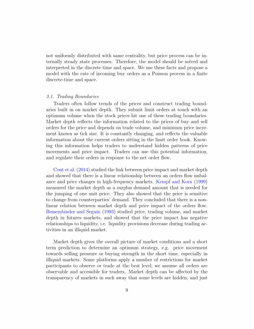
Plotting the trading boundaries (figure 8) shows that the optimal tradinglevel depends on the price process, the remainder of the inventory, and time

30

to maturity.

Due to market’s conditions and asset’s characteristics, an agent with thehigher degree of risk aversion, cares more about the execution risk and pricefluctuations. She starts the trading with available orders at a deeper level ofthe limit order book to avoid the risk execution and lack of offers in the future.She splits the original order into smaller slices to mitigate price impacts.

(a) (b)

Figure 7: (a): Inventory level of a trader with given the initial inventoryQ0 and time to maturity T, (b): Trading rate of liquidation problem withconstant order size 4

Table 1 summarizes results of simulations by our model, including the levelof inventory and its corresponding optimal trading rate for different scenariosof implementations of strategies. In the case of coming of not favorite offers,the algorithm reduces the speed of trading (panel I: self-damping property)and waited for a longer time to find better matching counterparties. In un-stable market conditions, are indicated with the higher level of self-damping,the trader should pay for final inventory to liquidate the whole position ofinitial shares. At this point, the best strategy is to accept offers in the limitorder book to avoid to never face severity penalties at the end of period. Ifestimated parameters of markets might show that the higher chance of same

31

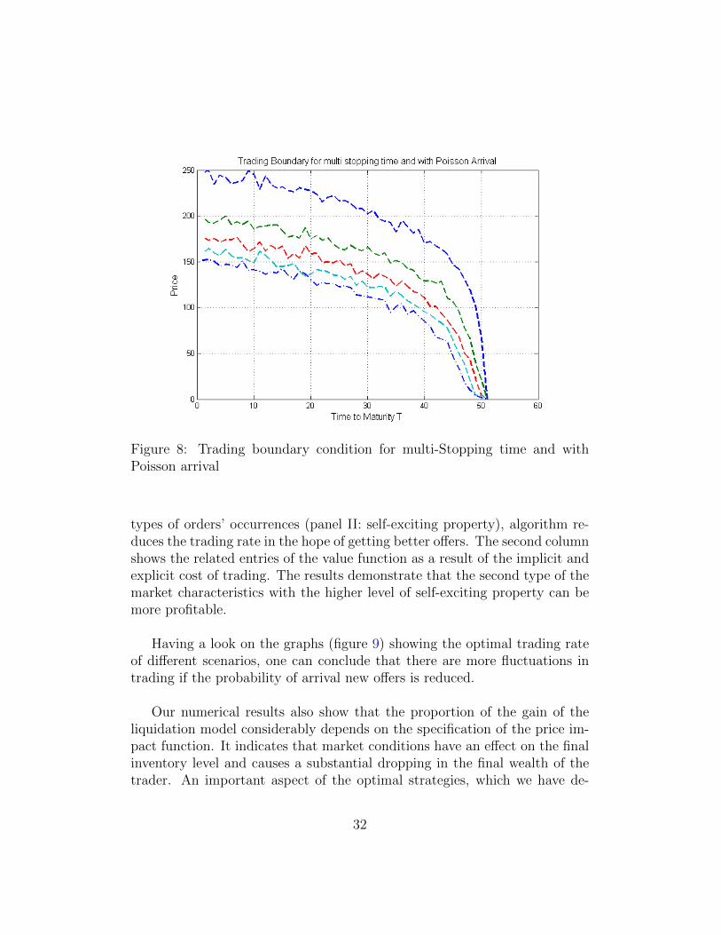
Figure 8: Trading boundary condition for multi-Stopping time and withPoisson arrival

types of orders’ occurrences (panel II: self-exciting property), algorithm re-duces the trading rate in the hope of getting better offers. The second columnshows the related entries of the value function as a result of the implicit andexplicit cost of trading. The results demonstrate that the second type of themarket characteristics with the higher level of self-exciting property can bemore profitable.

Having a look on the graphs (figure 9) showing the optimal trading rateof different scenarios, one can conclude that there are more fluctuations intrading if the probability of arrival new offers is reduced.

Our numerical results also show that the proportion of the gain of theliquidation model considerably depends on the specification of the price im-pact function. It indicates that market conditions have an effect on the finalinventory level and causes a substantial dropping in the final wealth of thetrader. An important aspect of the optimal strategies, which we have de-

32

Panel I QuantileSelf-damping Revenue 10% 25% 50% 75 % 100%κ = 0.6 $50,067 Trad˙rate 0.36 6.17 12.75 19.28 44.16σ = −0.6 Inven˙level 6205.45 14980.97 22618.06 31680.03 70000κ = 0.2 $50,352 Trad˙rate 0.27 5.69 11.92 19.09 44.59σ = −0.1 Inven˙level 6479.85 15814.89 23071.59 31534.80 70000κ = 0.6 $50,000 Trad˙rate 0.13 5.53 11.36 21.00 40.38σ = −0.1 Inven˙level 4159.49 14490.57 20724.59 30499.13 70000

Panel II QuantileSelf-exciting Revenue 10% 25 % 50% 75% 100%κ = 0.6 $50,779 Trad˙rate 0.59 6.17 12.54 19.27 43.20σ = 0.1 Inven˙level 3229.40 14751.81 22830.39 30507.01 70000κ = 0.2 $62,539 Trad˙rate 0.03 5.74 13.16 22.15 48.74σ = 0.1 Inven˙level 1593.42 11177.87 18155.91 31810.18 70000κ = 0.6 $94,691 Trad˙rate 0.34 9.68 16.12 26.71 72.67σ = 0.6 Inven˙level 2153.13 7580.03 19473.28 36405.45 70000

Table 1: Summary of the result of simulation the level of inventory and itscorresponding optimal trading rate under different market conditions

veloped, is to take into account the execution risk in an illiquid market i.e.inability to liquid shares at the given time.

The main assumption of the majority of limit order models is to trade atbest bid and ask prices (see: Cao et al. (2008), Battalio et al. (2014)). Weallow the trading procedure go to deeper into the limit order book to avoidnot filling the order and face last minute inventory penalties.

8. Discussion and Further works

In this paper, we proposed an analytical solution for the optimal liqui-dation problem with a dynamic approach and build numerical boundariesof multi-stopping problems in an illiquid market. We simulated the opti-mal splitting orders models according to the existing liquidity in the orderbook with different parameters and price impact models. We have used aPiecewise Deterministic Markov Decision Model (PDMD) to decompose the

33

Figure 9: Trading rate of liquidation Problem with different specification

liquidation problem, as a continuous-time stochastic control problem, intodiscrete period problems and applied Markov decision rules to obtain thesolution. We studied the uniqueness and existence of the optimal solution.We indicated that that the percentage gain of the liquidation model dependson the market conditions and specification of the price impact function.

In direct opposition to majority the limit order models for liquidatingmarket which only trading at best bid and ask prices, our model allows thetrading to go deeper into limit order book to avoid not filling of the orderand face last minute inventory punishment.

We believe that an attractive extension of our work would be to study;Cartea and Jaimungal (2014) discussed sophisticated models to trade at mar-ket order and post limit order; Cartea et al. (2014a) found optimal combi-nations of market and limit orders with learning from market dynamics totrade in the direction of price fluctuations.

Modeling the orders’ arrival flow with a Poisson process is quite robust ap-proach. Cartea et al. (2013) addressed several uncertainties about the arrivalrate of orders, the risk of not filling with limit orders, and misspecification inthe dynamics of the stock’s midprice, with the robust portfolio optimization

34

approach. Iyengar (2005) proposed a robust formulation which is systemat-ically alleviated the sensitivity of the Markovian policy on the uncertaintyof transition probabilities. We would like to examine the robustness of ourfindings with relaxing some assumptions of the model.

35

Reference

References

A. Alfonsi and A. Schied. Optimal trade execution and absence of pricemanipulations in limit order book models. SIAM Journal on FinancialMathematics, 1(1):490–522, 2010. doi: 10.1137/090762786. URL http:

//dx.doi.org/10.1137/090762786.

Aurelien Alfonsi and Pierre Blanc. Dynamic optimal execution in a mixed-market-impact hawkes price model. arXiv preprint arXiv:1404.0648, 2014.

Aurelien Alfonsi, Antje Fruth, and Alexander Schied. Constrained portfolioliquidation in a limit order book model. Banach Center Publ, 83:9–25,2008.

Aurelien Alfonsi, Antje Fruth, and Alexander Schied. Optimal executionstrategies in limit order books with general shape functions. QuantitativeFinance, 10(2):143–157, 2010.

Robert Almgren and Neil Chriss. Optimal execution of portfolio transactions.Journal of Risk, 3:5–40, 2001.

Marco Avellaneda and Sasha Stoikov. High-frequency trading in a limit orderbook. Quantitative Finance, 8(3):217–224, 2008.

E. Bacry, K. Dayri, and J.F. Muzy. Non-parametric kernel estimation forsymmetric hawkes processes. application to high frequency financial data.The European Physical Journal B, 85(5):157, 2012. ISSN 1434-6028. doi:10.1140/epjb/e2012-21005-8. URL http://dx.doi.org/10.1140/epjb/

e2012-21005-8.

E. Bacry, S. Delattre, M. Hoffmann, and J. F. Muzy. Modelling mi-crostructure noise with mutually exciting point processes. QuantitativeFinance, 13(1):65–77, 2013. doi: 10.1080/14697688.2011.647054. URLhttp://dx.doi.org/10.1080/14697688.2011.647054.

Vlad Bally, Gilles Pages, et al. A quantization algorithm for solving mul-tidimensional discrete-time optimal stopping problems. Bernoulli, 9(6):1003–1049, 2003.

36

Vlad Bally, Jacques Printems, et al. A quantization tree method for pricingand hedging multidimensional american options. Mathematical finance, 15(1):119–168, 2005.

Robert H Battalio, Shane A Corwin, and Robert H Jennings. Can brokershave it all? on the relation between make take fees & limit order executionquality. On the Relation between Make Take Fees & Limit Order ExecutionQuality (March 5, 2014), 2014.

Nicole Bauerle and Ulrich Rieder. Mdp algorithms for portfolio optimizationproblems in pure jump markets. Finance and Stochastics, 13(4):591–611,2009.

Erhan Bayraktar and Michael Ludkovski. Liquidation in limit order bookswith controlled intensity. Mathematical Finance, 24(4):627–650, 2014.

Erhan Bayraktar, Ulrich Horst, and Ronnie Sircar. Queueing theo-retic approaches to financial price fluctuations. Papers math/0703832,arXiv.org, March 2007. URL http://ideas.repec.org/p/arx/papers/

math-0703832.html.

Dimitri P.. Bertsekas and Steven Eugene Shreve. Stochastic optimal control:The discrete time case. Athena Scientific, 1996.

Dimitris Bertsimas and Andrew W Lo. Optimal control of execution costs.Journal of Financial Markets, 1(1):1–50, 1998.

Hendrik Bessembinder and Paul J Seguin. Price volatility, trading volume,and market depth: Evidence from futures markets. Journal of financialand Quantitative Analysis, 28(01):21–39, 1993.

Charles Cao, Oliver Hansch, and Xiaoxin Wang. Order placement strategiesin a pure limit order book market. Journal of Financial Research, 31(2):113–140, 2008.

Alvaro Cartea and Sebastian Jaimungal. Optimal execution with limit andmarket orders. Forthcoming: Quantitative Finance, 2014.

Alvaro Cartea, Ryan Donnelly, and Sebastian Jaimungal. Robust marketmaking. Available at SSRN 2310645, 2013.

37

Alvaro Cartea, Sebastian Jaimungal, and Damir Kinzebulatov. Algorithmictrading with learning. Available at SSRN 2373196, 2014a.

Alvaro Cartea, Sebastian Jaimungal, and Jason Ricci. Buy low, sell high: Ahigh frequency trading perspective. SIAM Journal on Financial Mathe-matics, 5(1):415–444, 2014b.

R. Cont. Statistical modeling of high-frequency financial data. Signal Pro-cessing Magazine, IEEE, 28(5):16–25, Sept 2011. ISSN 1053-5888. doi:10.1109/MSP.2011.941548.

Rama Cont and David-Antoine Fournie. Change of variable formulas for non-anticipative functionals on path space. Journal of Functional Analysis, 259(4):1043–1072, 2010.

Rama Cont, Sasha Stoikov, and Rishi Talreja. A stochastic model for orderbook dynamics. Operations Research, 58(3):549–563, 2010. doi: 10.1287/opre.1090.0780. URL http://dx.doi.org/10.1287/opre.1090.0780.

Rama Cont, Arseniy Kukanov, and Sasha Stoikov. The price impact of orderbook events. Journal of financial econometrics, 12(1):47–88, 2014.

Mark HA Davis. Piecewise-deterministic markov processes: A general classof non-diffusion stochastic models. Journal of the Royal Statistical Society.Series B (Methodological), pages 353–388, 1984.

Benoıte De Saporta, Francois Dufour, Karen Gonzalez, et al. Numericalmethod for optimal stopping of piecewise deterministic markov processes.The Annals of Applied Probability, 20(5):1607–1637, 2010.

Robert F Engle and Asger Lunde. Trades and quotes: a bivariate pointprocess. Journal of Financial Econometrics, 1(2):159–188, 2003.

Mark B. Garman. Market microstructure. Journal of Financial Economics,3(3):257 – 275, 1976. ISSN 0304-405X. doi: http://dx.doi.org/10.1016/0304-405X(76)90006-4. URL http://www.sciencedirect.com/science/

article/pii/0304405X76900064.

Jim Gatheral. No-dynamic-arbitrage and market impact. QuantitativeFinance, 10(7):749–759, 2010. URL http://EconPapers.repec.org/

RePEc:taf:quantf:v:10:y:2010:i:7:p:749-759.

38

Olivier Gueant, Charles-Albert Lehalle, and Joaquin Fernandez-Tapia. Op-timal portfolio liquidation with limit orders. SIAM Journal on FinancialMathematics, 3(1):740–764, 2012.

ALAN G. HAWKES. Spectra of some self-exciting and mutually excitingpoint processes. Biometrika, 58(1):83–90, 1971. doi: 10.1093/biomet/58.1.83. URL http://biomet.oxfordjournals.org/content/58/1/83.

abstract.

Ulrich Horst and Felix Naujokat. On derivatives with illiquid underlying andmarket manipulation. Quantitative Finance, 11(7):1051–1066, 2011.

Ulrich Horst and Felix Naujokat. When to cross the spread? trading in two-sided limit order books. SIAM Journal on Financial Mathematics, 5(1):278–315, 2014.

Garud N Iyengar. Robust dynamic programming. Mathematics of OperationsResearch, 30(2):257–280, 2005.

Alexander Kempf and Olaf Korn. Market depth and order size. Journal ofFinancial Markets, 2(1):29–48, 1999.

Albert S Kyle. Continuous auctions and insider trading. Econometrica:Journal of the Econometric Society, pages 1315–1335, 1985.

D. V. Lindley. Dynamic programming and decision theory. Journal of theRoyal Statistical Society. Series C (Applied Statistics), 10:39–51, 1961.

Francis A Longstaff and Eduardo S Schwartz. Valuing american options bysimulation: A simple least-squares approach. Review of Financial studies,14(1):113–147, 2001.

Ragnar Norberg. Vasicek beyond the normal. Mathematical Finance, 14(4):585–604, 2004.

T. Ozaki. Maximum likelihood estimation of hawkes’ self-exciting pointprocesses. Annals of the Institute of Statistical Mathematics, 31(1):145–155, 1979. ISSN 0020-3157. doi: 10.1007/BF02480272. URL http:

//dx.doi.org/10.1007/BF02480272.

39

Goran Peskir and Albert Shiryaev. Optimal stopping and free-boundaryproblems. Optimal Stopping and Free-Boundary Problems, pages 123–142,2006.

S. Predoiu, G. Shaikhet, and S. Shreve. Optimal execution of a generalone-sided limit-order book. SIAM Journal on Financial Mathematics, 2:183–212, 2011.

Eric Smith, J Doyne Farmer, Laszlo Gillemot, and Supriya Krishna-murthy. Statistical theory of the continuous double auction. Quantita-tive Finance, 3(6):481–514, 2003. URL http://ideas.repec.org/a/taf/

quantf/v3y2003i6p481-514.html.

40

9. Appendix

Proof of Theorem 1. If the number of orders is a random variable with thePoisson distribution and the mean value λ in a finite interval of length t. Weconsider the order with maximum price of N (0,t) number of limit orders as:

Y = maxS1t , · · · , SN

(0,t)

t

We define FN(0,t)(Y )

FN(0,t)(Y ) = P [(S1 ≤ Y ) ∩ (S2 ≤ Y )∩, · · · , SN ≤ Y )]

= F (Y )N(0,t)

The generating function with distribution function F (St) is

Gt(F (y)) = E[F (Y )N(0,t)

]

Gt+dt(F (Y )) = E[F (Y )N(0,t+dt)

]

= E[F (Y )N(0,t)+N(t,t+dt)

]

= E[F (Y )N(0,t)E[F (Y )N

(t,dt)

]

= Gt(F (Y ))(1− λdt+ λdt.F (Y ))

Gt+dt(F (Y ))−Gt(F (Y ))

dt= −λ(1− F (Y ))Gt(F (Y ))

d

dt(Gt(F (Y )) = −λ(1− F (Y ))Gt(F (Y ))

d

dtln(Gt(F (Y )) = −λ(1− F (Y ))

Gt(F (Y )) = e−λt(1−F (Y ))

41

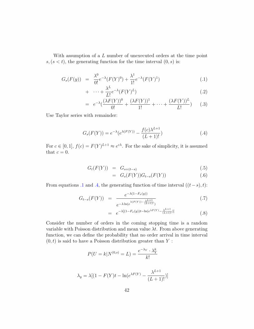
With assumption of a L number of unexecuted orders at the time points, (s < t), the generating function for the time interval (0, s) is:

Gs(F (y)) =λ0

0!e−λ(F (Y )0) +

λ1

1!e−λ(F (Y )1) (.1)

+ · · ·+ λL

L!e−λ(F (Y )L) (.2)

= e−λ((λF (Y ))0

0!+

(λF (Y ))1

1!+ · · ·+ (λF (Y ))L

L!) (.3)

Use Taylor series with remainder:

Gs(F (Y )) = e−λ(eλ(F (Y )) − f(c)λL+1

(L+ 1)!) (.4)

For c ∈ [0, 1], f(c) = F (Y )L+1 ≈ ecλ. For the sake of simplicity, it is assumedthat c = 0.

Gt(F (Y )) = Gs+(t−s) (.5)

= Gs(F (Y ))Gt−s(F (Y )) (.6)

From equations .1 and .4, the generating function of time interval ((t−s), t):

Gt−s(F (Y )) =e−λ(1−Fx(y))

e−λ ln(eλ(F (Y ))− λL+1

(L+1)! )

(.7)

= e−λ[(1−Fx(y))t−ln(eλF (Y )− λL+1

(L+1)!)] (.8)

Consider the number of orders in the coming stopping time is a randomvariable with Poisson distribution and mean value λt. From above generatingfunction, we can define the probability that no order arrival in time interval(0, t) is said to have a Poisson distribution greater than Y :

P (U = k|N (0,s) = L) =e−λY · λkY

k!

λy = λ[(1− F (Y )t− ln(eλF (Y ) − λL+1

(L+ 1)!)]

42

where F (Y ) is the distribution of the price process and L is the number ofunexecuted orders up to time point s. Where k = 0 , it gives the probabilityof the best order, k = 1 is the second the best order, etc.

Proof of Lemma 2. It is assumed the limit orders arrival rate is a point pro-cess with intensity rate λt and we liquidate 4γt at each stopping time:τ = 0 < T1 < T2 < · · · < Tn ≤ T

V (T,Q0) = supγ∈A

Et,q[V (T,Q0)]

= supγ∈A

Et,q[n∑i=1

e−rTi 4 γtSt1(Ti≤T )]

(when n→∞)(t ∈ τ) = supγ∈A

Et,q[∫ T ′

0

e−rt4 γtStdNt]

= supγ∈A

Et,q[∫ T ′

0

e−rt4 γtStλtdt]

Proof of Proposition 3. Following SDE represents the impact of trading onthe dynamics of the rate of orders’ arrival:

dλt = (f(γt)− κλt)dt+ σdNt (.9)

In order to prove, we can move the first term of SDE to the left side, thenmultiply it by eκt (see : Norberg (2004)) or alternatively we can define aninitial guess for the solution of above SDE as follows:

λt = λ0 +

∫ t

0

(f(γs)Γ(t− s))ds+ σ

∫ t

0

e−κ(t−s)dNs (.10)

43

Verify by Ito’s lemma on eκtλt

eκtλt = eκt∫ t

0

(f(τs)e−κ(t−s))ds+ eκtσ

∫ t

0

e−κ(t−s)dNs(.11)

=

∫ t

0

(f(γs)eκs)ds+ σ

∫ t

0

eκsdNs (.12)

κeκtλtdt+ eκtdλt = (f(γt)eκt)dt+ σeκtdNt (.13)

κλtdt+ dλt = (f(γt))dt+ σdNt (.14)

dλt = (f(γt)− κλt)dt+ σdNt (.15)

(.16)

Proof of Lemma 4. of a buy order (.10).

limt→∞

D(t) = limt→∞

∫ t

0

(f(γs)Γ(t− s))ds

= limt→∞

∫ t

0

(f(γs)e−κ(t−s))ds

= limt→∞

e−κt∫ t

0

(f(γs)eκs)ds

= limt→∞

∫ t0(f(γs)e

κs)ds

eκt

(apply l’Hopital’s rule) = limt→∞

(f(γt)eκt)

κeκt

= limt→∞

exp(αγt)

κ

= limt→∞

1 + αγt +O(αγt)

κ≈ 1 + αγT

κ= λ∞

We defined the liquidation problem as a finite time investing problem ona limited time horizon T . λ∞ represents the long run trading impact onthe intensity of order arrivals rate, we can think of it as a permanent priceimpact as ”base” intensity part of stochastic intensity. It is a linear functionof trading rate to avoid dynamic arbitrage Gatheral (2010). We can expressthe permanently effected stochastic intensity by:

44

λPermt = λ∞ + σ

∫ t

0

e−κ(t−s)dNs (.17)

Instantaneous market impacts can be measured from the small intervalof trading, and the difference between the pre-trade and post-trade pricemovements:

limε→0

D(t) = limε→0

∫ t+ε

t

(f(γs)Γ(t− s))ds

= limε→0

∫ t+ε

t

(exp(αγs)e−κ(t−s))ds ≈ exp(−κt+ αγε) = λε

We can simply define the instantaneously affected stochastic intensity by:

λInstt = λε + σ

∫ t

0

e−κ(t−s)dNs (.18)

Proof of Theorem 5. By using the information on the jump location fromZ = (Z1, Z2, · · · , Zn) as a set of post jump of PMDP , we have:

V π(t, q) = Et,q[∫ T ′

0

e−rt4 γtstλtdt] (t ∈ τ)

(refer to equation:6.3) = Et,x[∫ T ′

0

Uπ(XT ′)dNt]

= Et,x[N∑i=0

[

∫ Ti+1∧T ′

Ti

Uπ(φ(XTi))dNt]

(Zi define as Zi = [Ti, XTi ]) = Et,x[N∑i=0

Et[∫ Ti+1∧T ′

Ti

Uπ(φ(XTi))dNt|Zi]]

= Et,x[N∑i=0

R(Zi, πi(Zi))]

= Ψπ(t, x)

45

We define a set Π = π1, π2, · · · , πN as a sequence of all Markovian decisioncontrols πi corresponding to the Markovian policy for the predictable admis-sible process γ included in the set Ψ. We can then decompose this optimalcontrol problem into the piecewise-deterministic Markov process:

V (t, q) = supπ∈Π

Ψ(t, x)

Proof of Theorem 6. In the theorem 5, we have shown that

V (t, q) = supγHγ(t, q)

= supπ∈Π

Ψπ(t, x)

with defining the sequence of Π = π1, π2, · · · , πn as set of Markovian poli-cies (Bertsekas and Shreve (1996)), we have:

Ψπn = limn→+∞

T π0 · T π1 · T π2 · · · T πn−1Ψπ0(x0)

= limn→+∞

(T πn)n(Ψπ0(x0))

= T n(Ψπn(x0))

Therefore under the same condition, the optimal solution is defined as:

Ψ(x) = supπ∈Π

(Ψπ(x))

Equally

Ψ(x) = T (Ψ(x))

which is a subset of the Banach space, so we can apply the Banach fixedpoint theorem and show that V is an unique fixed point of the operator Ton the set Π.

46