option-implied risk-neutral distributions and risk aversion · finally, option-pricing theory...
TRANSCRIPT

The Research Foundation of AIMR™
RE
SE
AR
CH
FOUN
DA
TIO
N
OF A I M R
Jens Carsten JackwerthUniversity of Konstanz
Germany
Option-ImpliedRisk-Neutral Distributionsand Risk Aversion
The Research Foundation of The Association for Investment Management and Research™,the Research Foundation of AIMR™, and the Research Foundation logo are trademarksowned by the Research Foundation of the Association for Investment Management andResearch. CFA®, Chartered Financial Analyst®, AIMR-PPS®, and GIPS® are just a few of thetrademarks owned by the Association for Investment Management and Research. To view alist of the Association for Investment Management and Research’s trademarks and a Guide forthe Use of AIMR’s Marks, please visit our website at www.aimr.org.
© 2004 The Research Foundation of the Association for Investment Management and Research
All rights reserved. No part of this publication may be reproduced, stored in a retrieval system, or transmitted, in any form or by any means, electronic, mechanical, photocopying, recording, or otherwise, without the prior written permission of the copyright holder.
This publication is designed to provide accurate and authoritative information in regard to the subject matter covered. It is sold with the understanding that the publisher is not engaged in rendering legal, accounting, or other professional service. If legal advice or other expert assistance is required, the services of a competent professional should be sought.
ISBN 0-943205-66-2
Printed in the United States of America
March 31, 2004
Editorial Staff Elizabeth A. Collins
Book Editor
Sophia E. BattagliaAssistant Editor
Kara H. MorrisProduction Manager
Lois A. Carrier/Jesse KochisComposition and Production

Mission
The Research Foundation’s mission is to encourage education for investment practitioners worldwide and to fund, publish, and distribute relevant research.
Biography
Jens Carsten Jackwerth is a professor of economics at the University ofKonstanz, Germany. He was a visiting postdoctoral scholar at the Universityof California at Berkeley until 1997 and taught at the London BusinessSchool until 1999 and then at the University of Wisconsin at Madison beforetaking his current position in 2001. His research interests are derivativespricing and asset pricing—in particular, how to unlock the informationcontained in option prices to gain insight into the underlying probabilitiesand beliefs held by market participants. In related research, ProfessorJackwerth has investigated stochastic processes for stock prices that areconsistent with observed option prices. His work has appeared in theJournal of Finance, Review of Financial Studies, Journal of PortfolioManagement, and Journal of Derivatives. Professor Jackwerth received hisPhD in finance from Göttingen University in 1994.
Contents
Foreword . . . . . . . . . . . . . . . . . . . . . . . . . . . . . . . . . . . . . . . . . . . . . . vi
Preface . . . . . . . . . . . . . . . . . . . . . . . . . . . . . . . . . . . . . . . . . . . . . . . . viii
Option-Implied Risk-Neutral Distributions and Risk Aversion . . 1
Appendix A: Fast and Stable Method . . . . . . . . . . . . . . . . . . . . . . . 65
Appendix B: Derman–Kani Implied Binomial Tree . . . . . . . . . . . 67
Glossary . . . . . . . . . . . . . . . . . . . . . . . . . . . . . . . . . . . . . . . . . . . . . . . 71
References . . . . . . . . . . . . . . . . . . . . . . . . . . . . . . . . . . . . . . . . . . . . . 74
vi ©2004, The Research Foundation of AIMR™
Foreword
The development of option-pricing theory is perhaps the most significantachievement in financial economics, if not all of economics. Moreover, it hasa wonderfully rich history, parts of which are recounted here. Long beforeFischer Black and Myron Scholes and Robert Merton nailed it, luminaries suchas the French mathematician Louis Bachelier, the brilliant economist Paul A.Samuelson, and the famous card counter Ed Thorp contributed to the ultimatesolution. And let’s not forget Albert Einstein, whose unwitting contribution tooption-pricing theory through his exploration of Brownian motion was citedas one of the key contributions that led to his Nobel Prize in physics.
Option-pricing theory is significant not only for the intellectual advancesit inspired, however, but also because it contributes to social amenity—perhaps more so than some of the more obvious and heralded achievementsin the natural sciences. Options afford producers and service providers amechanism to hedge risk, which allows them to offer their products andservices at lower prices than they would otherwise require. A robust option-pricing framework facilitates these hedging activities and, therefore, pro-motes broad access to critical goods and services.
Finally, option-pricing theory offers a prism by which valuable informationabout expectations and risk preferences is revealed to us, which is the topicof this fine Research Foundation monograph by Jens Carsten Jackwerth.Investors have long used option prices to infer market expectations about thevolatilities and correlations of the underlying assets. After the stock marketcrashed in 1987, investors and researchers noticed that the volatilities impliedby option prices on the same underlying asset differed depending on the strikeprices of the option contracts. The initial approach for reconciling thesedifferences was to depart from the standard assumption that returns arelognormally distributed and, instead, infer the distribution that would give riseto these differences in implied volatilities. A subsequent approach has beento attribute the differences in implied volatilities to the differences in riskpreferences.
Jackwerth presents both approaches and in a style that is rigorous but,despite the technical nature of the material, readily accessible to practitioners.Moreover, Jackwerth, unlike the quintessential ivory tower academic whoviews the real world as an uninteresting, special case of his model, takes careto offer many practical insights into how practitioners can use this informationto improve their understanding of markets.
Although this material is not light reading, Jackwerth is particularlyconsiderate of the nonexpert in two ways. He offers a glossary of technical
Foreword
©2004, The Research Foundation of AIMR™ vii
terms, and he collects the seriously technical material in two appendixes.Whether you specialize in options trading or simply want a better understand-ing of some of the fascinating world of options, you will be very well servedby this excellent monograph. The Research Foundation is especially pleasedto present Option-Implied Risk-Neutral Distributions and Risk Aversion.
Mark Kritzman, CFAResearch Director
The Research Foundation of theAssociation for Investment Management and Research
viii ©2004, The Research Foundation of AIMR™
Preface
Since about 1994, considerable interest has been shown in academia and thecentral banks in “option-implied risk-neutral distributions.” The purpose ofthis Research Foundation monograph is to provide some insight into the useof such a concept for the investment professional. Much of the work in thisfield is mathematically complex, requires advanced tools of financialeconomics, and is written with fellow researchers rather than practitioners inmind. The goal of this monograph is to bridge the gap between academia andpractice by explaining what can and what cannot be learned from option pricesfor applications in financial analysis. As part of this goal, I provide step-by-stepexamples so that the reader can actually apply these concepts.
Fundamentally, the concept of learning from option prices, which under-lies the estimation of the risk-neutral distribution, is not new. Investmentprofessionals have always appreciated prices for the information they contain.For example, a high price of IBM shares compared with their historical levelsindicates that investors value IBM highly. We might not know why, but thatinformation alone (that other investors think highly of IBM) is important newsto us. Consider a different example: If we know the value of futures contractswritten on an index and know the value of the index (because shares histori-cally did not have futures written on them), we can also infer the risk-freeinterest rate as the ratio of the futures value and ex dividend index value.Similarly, we have long been accustomed to using bond prices to infer theterm structure of spot and forward rates, from which we can speculate aboutfuture spot interest rates. In this case, we are learning from each bond priceabout a particular interest rate.
We can think of security prices as some kind of expected value of futurecash flows (the exact nature of the expectation is at this point irrelevant forthe argument, and I will address it later in great detail). Then, each price tellsus a little bit about the probability distribution from which we take thoseexpectations. One price (say, the futures price) will yield one piece of infor-mation about the probability distribution. In the simple case of only one futuresprice, the price information will yield the location of that distribution—that is,the expected value that is the risk-free rate in this example. That the expectedreturn under our distribution is the risk-free rate, not the mean index return,might come as a surprise. The explanation is that for pricing purposes, we usea different distribution from the actual probability distribution; we use the risk-neutral distribution. I return to the exact nature of this risk-neutral distributionin the following pages.

Preface
©2004, The Research Foundation of AIMR™ ix
When we are able to examine option prices in addition to the stock price,we gain with each option price one more piece of information about the risk-neutral probability distribution. For example, with four options written on ashare, all of which expire at the same time but all of which have different strikeprices, we have information about four moments of the distribution—quite alot of information, which we can use to depict the risk-neutral distribution. So,although learning from prices about the location of the distributions of futuresecurity prices is an old concept, its application to options is new and rich.Options allow us to learn much more about the shape of the risk-neutraldistribution.
A final application is to compare the option-inferred risk-neutral distribu-tions with estimated actual distributions of stock prices based on, for example,the historical price path. The relationship between these two distributionsdepends on the preferences (utilities) of investors about money as they growricher or poorer. Knowing both distributions allows us to infer what thepreferences must be within an economy to be consistent with option pricesand historical returns.
Where does all this research and information leave the investment pro-fessional? Although a great deal can be learned from option prices, we needto establish what can be reasonably well analyzed (the center of the option-implied risk-neutral probability distribution) and what cannot (individualpreferences or actual movements of security prices). What this monographtries to achieve is a clear demonstration for practitioners of what can bereasonably inferred from option prices, how to do that, and what pitfalls toavoid. Another issue is the interpretation of this information. If we are observ-ing only the risk-neutral distribution, we must be careful not to immediatelyapply it for forecasting actual events. For such forecasts, the actual distributionmust be used. So, the monograph will detail the rules governing when andhow to use the option-implied risk-neutral distribution. Finally, the monographunveils an empirical irregularity, the “pricing kernel puzzle,” which suggeststhat the risk-neutral distribution, the actual distribution, and the impliedpreferences are incompatible with each other. An implication of this puzzle isthat money can be made if some securities are mispriced. I spell out in detailwhat kinds of strategies may be profitable.
I usually identify terms as the discussion develops, but because a numberof the terms in the monograph might not be familiar to the reader, I havecollected them in a glossary that briefly explains each one. Terms that areincluded in the glossary are in small capital letters when they are firstmentioned in the text or exhibits.

Option-Implied Risk-Neutral Distributions and Risk Aversion
x ©2004, The Research Foundation of AIMR™
This monograph is organized in the following manner. First, I discuss whyfinancial analysts might be interested in learning about the economy fromoption prices. I also provide a brief history of option pricing. Next, themonograph explores the empirical problems of the Black–Scholes (1973)model, especially after the 1987 market crash, and investigates potentialexplanations for the behavior of observed option prices. The monograph thenintroduces risk-neutral option pricing and the theoretical underpinnings ofasset pricing in complete and incomplete markets. The concept of the risk-neutral probability distribution formally introduced at this point is central tothe rest of the monograph. The stage is now set for a thorough discussion ofthe “inverse problem,” which concerns how to obtain risk-neutral implieddistributions from observed market option prices. Then, the discussion turnsto the question of what stochastic processes are consistent with a particularterminal risk-neutral distribution. Binomial trees are particularly simple exam-ples of such stochastic processes, but I also present extensions and alternativeapproaches. By building on the theory presented earlier, I can now use theratio of the risk-neutral implied distribution and the actual distribution toestimate economywide scaled marginal utility functions (pricing kernels), amethodology that is described thoroughly before the concluding section.
For helpful discussions related to the monograph, I would like to thankKostas Iordanidis and Mark Rubinstein. Generous funding by the AIMRResearch Foundation is gratefully acknowledged. I am also thankful to MarkKritzman, the Foundation’s research director. This monograph is based inpart on an earlier article (Jackwerth 1999), and I am grateful to InstitutionalInvestor for permission to use the 1999 article in this way.
©2004, The Research Foundation of AIMR™ 1
Option-Implied Risk-Neutral Distributions and Risk Aversion
In introducing the motivation behind this monograph, I would like to turnusual security valuation and OPTION-pricing theory upside down. For thelongest time, practitioners and academics were content with pricing securitiesbased on models that made specific assumptions about the evolution ofsecurity prices. Often, we assumed a GEOMETRIC BROWNIAN MOTION to describesecurity prices. The resulting model-based security prices were then used fortrading.1 But traders soon realized that some market prices did not adhere tothe model prices. Rubinstein (1985) documented the first such widespreadviolations of model prices. We came to realize that our stylized models do notaccount for all facets of the real world. The fact that the real world is muchricher in patterns and processes seems obvious, but only recently has thisappreciation been translated into reversing the direction of reasoning: It is nolonger from an assumed model toward theoretical prices but from observedmarket prices to the implied distributions and STOCHASTIC processes that couldhave generated them.
The reasons for this change in perspective are manifold. For one, our trustin market prices increased as exchanges became more common and morereliable. Data are more widely available nowadays. Especially for equityoptions, researchers detected pronounced deviations of observed prices frommodel prices starting after the crash of 1987. Finally, mathematical sophisti-cation and computational power became available to tackle the so-calledinverse problem: What information about the economy and security processesis contained in a set of market prices?
Before venturing to answer that question, I would like to spend some timeon the history of option pricing up to the turning point—that is, the crash of1987.2 Options have been with us for a long time. One of the first examplescomes from around 550 B.C. in ancient Greece, where CALL OPTIONS on olivepresses gave the owner of the options, Thales of Miletus, the right to use allthe olive-pressing capacity in Chios and Miletus after the harvest. Throughmost of history, options were traded—as in the 1870s in New York, for
1In the case of options, these models would begin with the famous Black–Scholes (1973) modelfor pricing options.2More detailed accounts can be found in Benhamou (2003) and Margrabe (2002).
Option-Implied Risk-Neutral Distributions and Risk Aversion
2 ©2004, The Research Foundation of AIMR™
example—between buyers and sellers as over-the-counter instruments. Someexchanges, however, traded options as early as the 17th century (Amster-dam), and Bachelier (1900) reported option trading on the Paris exchangearound 1900. The situation changed fundamentally on 26 April 1973, when theChicago Board Options Exchange (CBOE) introduced exchange-tradedoptions. Trading volume grew rapidly, and other exchanges were soon alsooffering option contracts.
Analysis of the pricing of options largely paralleled this development. Inthe beginning, investors had to think about how much an option would beworth to them without the benefit of a mathematical model; prices tended tobe the result of educated guesses, because liquid markets did not exist. Pricesof options were higher than would be produced from modern models andhigher than present-day market prices, indicating the presence of a substantialRISK PREMIUM to compensate the writer of the option for the trouble of providingsuch a rare security that was so difficult to value.
Bachelier was the first to develop a theoretical model to price options.Having been a student of the mathematician Poincare, he assumed that a stockprice evolves over time as an arithmetic BROWNIAN MOTION. The requiredassumptions were themselves problematic; they stipulated normally distrib-uted stock prices that could become negative and ignored dividends andinterest rates. Despite these drawbacks, his work was far ahead of its timebecause it was based on probabilistic assumptions about the evolution of stockprices. Nobody else thought in such a way about stock prices at the time, andhis thesis was promptly forgotten until the middle of the 20th century.
At that time, Osborne (1959) advocated geometric Brownian motion asthe model for asset prices. At this point, a mathematical model of optionpricing could finally be derived. Under the assumption of geometric Brownianmotion, we know that the stock price at some terminal date will be lognormallydistributed. Also, we can calculate the payoff of the option for each realizationof the underlying stock price. We can then calculate the expected payoff ofthe option by multiplying each payoff at a given stock price by the likelihoodof that payoff occurring and subsequently summing across all stock prices.
An important ingredient was still missing at this point. Bachelier com-pletely ignored appreciation of the stock, but simply using the expected rateof return on the stock is also not correct. The reason is that the utility of theinvestor—that is, the investor’s attitude toward risk taking—plays a role inpricing when risky payoffs are involved, as is the case with an option. The wayrisk-averse investors treat an additional dollar depends on the investors’wealth at any time. When investors are poor, they will pay more for thatadditional dollar than when they are rich. These concepts were developed for

Option-Implied Risk-Neutral Distributions and Risk Aversion
©2004, The Research Foundation of AIMR™ 3
financial applications starting in the late 1950s by, among others, Sharpe(1964) and Samuelson (1965). Incorporating utility theory’s concept of riskaversion is an essential part of Sprenkle’s (1964) option-pricing formula:
(1)
where C = value of the call optionρ = average rate of growth of the share priceT = time to maturity of the optionS = share priceN(⋅) = cumulative standard normal distribution functionK = exercise price of the optionσ = volatility of the stock returnsZ = degree of risk aversionSlightly varying models were built by Boness (1964), Samuelson, and
Thorp and Kassouf (1967). The Sprenkle formula involved the expected return on the asset, r, and
incorporated an adjustment for risk aversion, Z. The formula was thusunwieldy because analysts normally do not know the economywide coefficientof risk aversion. Also, early investors realized that the Sprenkle formula didnot work well for pricing the existing options of the time. An ad hoc adjustmentcould be made, however, by setting risk aversion to zero, replacing theexpected return on the stock with the risk-free rate, and discounting theresulting option price at the risk-free rate.
Not until the seminal work of Black and Scholes and of Merton (1973),however, could analysts have a clear theoretical understanding of why therisk-free rate should be used for discounting instead of the expected returnon the asset. The short explanation is that in COMPLETE MARKETS, investors canhedge their exposure to an option by an offsetting position in the stock andthe bond. But if any investor can costlessly eliminate the risk of the optionposition, then the expected return should be only the risk-free rate.
Black developed this idea when he applied the capital asset pricing model(CAPM) to option pricing. He was pointed in this direction by Jack Treynor,who suggested the use of a Taylor series expansion. The personal riskaversion of the investor no longer mattered in this approach because any riskcould be hedged. In particular, Black and Scholes realized that the expectedreturn on the stock did not appear in the option-pricing formula anymore andcould thus be set to any value. The risk-free rate turned out to be a convenient
C e ρT S( )N S K⁄( )ln ρ σ2 2⁄+( )T+
σ T------------------------------------------------------------ 1 Z–( ) K( )N S K⁄( )ln ρ σ2 2⁄–( )T+
σ T------------------------------------------------------------ ,–=

Option-Implied Risk-Neutral Distributions and Risk Aversion
4 ©2004, The Research Foundation of AIMR™
choice because it represents how a risk-neutral investor would discount. Thus,the terms “risk-neutral pricing” and “risk-neutral distribution” were intro-duced. The resulting Black–Scholes formula is
(2)
where r is the risk-free interest rate.This formula was a breakthrough theoretically and in practical terms
because all inputs to the Black–Scholes formula were observable except theVOLATILITY parameter, which could be estimated from historical stock returns.3Merton’s particular contribution was to show mathematically how one canhedge all risks, not just the systematic risk of the CAPM with which Blackand Scholes were concerned. The explosive growth of the options industrywas fueled by the advent of large organized exchanges at the same time andthe development of an efficient numerical scheme by Cox, Ross, and Rubin-stein (1979). We will look at that scheme in more detail in the section “ImpliedBinomial Trees.”
In the wake of development of the Black–Scholes formula, many exten-sions were proposed. Almost immediately, Merton introduced models thatincorporated stochastic interest rates, dividends, changes in STRIKE PRICES,American-style exercise before expiration, and a down-and-out call. Otherextensions involved applications to corporate debt, futures, currencies,options to exchange one asset for another, options on the minimum andmaximum of several assets, and a variety of other specialized options. Twomore modern developments came with the introduction of stochastic volatilityby Heston (1993) and the addition of stochastic jumps and stochastic interestrates by Bates (1996, 2000, 2001).
The basic modeling direction, however, was not fundamentally changed.Researchers always started out with a stochastic process that described theevolution of the underlying asset. Then, they worked out the risk-neutraldynamics of that stochastic process (e.g., changing the discount rate from theexpected return on the asset in the Sprenkle formula to the risk-free rate inthe Black–Scholes case). The final option-pricing model was then the dis-counted expected value of the option payoff under the RISK-NEUTRAL PROBABILITY
distribution.This way of thinking changed with the advent of exchange-traded options
in the early 1970s. As option prices became available in large quantities,
3Merton and Scholes received the Nobel Prize for the pricing model in 1997; Black’s death in1995 prevented him from joining his colleagues.
C S( )N S K⁄( )ln r σ2 2⁄+( )T+
σ T----------------------------------------------------------- e rT– K( )N S K⁄( )ln r σ2 2⁄–( )T+
σ T----------------------------------------------------------- ,–=

Option-Implied Risk-Neutral Distributions and Risk Aversion
©2004, The Research Foundation of AIMR™ 5
investors began to reverse the process of obtaining prices from models toworking out the implied model parameters that were consistent with observedprices. They calculated implied Black–Scholes volatilities, which are neededas inputs to the Black–Scholes formula to arrive at the observed market prices.The IMPLIED VOLATILITY of an option is simply that volatility that makes themodel price exactly equal to the observed market price. Each option has aunique implied volatility, and traders like to quote options in terms of impliedvolatilities. The main reason is that as the underlying asset price changesthrough the day, the implied volatility does not have to be adjusted as muchas the option prices, which change all the time.
The only way to calculate implied volatilities is through an iterativeprocedure based on a Newton–Raphson search.4 Manaster and Koehler(1982) worked out the details and a starting value that guarantees conver-gence. Hentschel (2003) noted that implied volatilities suffer from biases ifoption prices are observed with such errors as finite quote precision, BID–ASK
SPREADS, or nonsynchronous prices. A further upward bias results from acensoring of low prices that violate no-arbitrage bounds. These problems aremost prevalent for away-from-the-money options, and Hentschel derived opti-mal weighting schemes to mitigate these errors in implied volatilities.
The novel aspect in calculating implied volatilities is that equilibriummarket prices are now being used to learn about the stochastic process of theunderlying asset and its probability distribution rather than this process beingassumed. This monograph investigates these recent developments anddescribes what we can learn from observed option prices about the economywe live in.
Empirical FindingsWe start with a description of the empirical regularities of the implied volatil-ities in different markets. Many of the results hint at the fact that the Black–Scholes model might not hold perfectly in the real world. Thus, we investigatepotential explanations for deviations from the Black–Scholes model.
Empirical Problems with Black–Scholes. Ever since investors havebeen calculating implied volatilities, they have also plotted them across strikeprices for options with the same time to expiration and on the same underlyingstock. These plots are called (implied) volatility “smiles.” According to theBlack–Scholes formula, the VOLATILITY SMILE should be a flat line because onlyone volatility parameter governs the underlying stochastic process on whichall options are priced. Rubinstein (1985) did indeed find that the volatility
4A Newton–Raphson search is an iterative procedure for finding the roots of a function.
Option-Implied Risk-Neutral Distributions and Risk Aversion
6 ©2004, The Research Foundation of AIMR™
smiles for options on individual U.S. stocks are more or less flat. Although hefound slightly U-shaped volatility smiles for individual stock options, theviolations of the Black–Scholes model were mainly within the bid–ask spreads.An investor would thus not be able to trade profitably on these deviations.
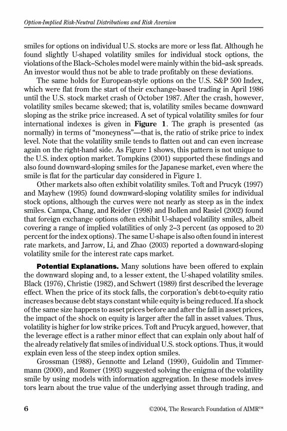
The same holds for European-style options on the U.S. S&P 500 Index,which were flat from the start of their exchange-based trading in April 1986until the U.S. stock market crash of October 1987. After the crash, however,volatility smiles became skewed; that is, volatility smiles became downwardsloping as the strike price increased. A set of typical volatility smiles for fourinternational indexes is given in Figure 1. The graph is presented (asnormally) in terms of “moneyness”—that is, the ratio of strike price to indexlevel. Note that the volatility smile tends to flatten out and can even increaseagain on the right-hand side. As Figure 1 shows, this pattern is not unique tothe U.S. index option market. Tompkins (2001) supported these findings andalso found downward-sloping smiles for the Japanese market, even where thesmile is flat for the particular day considered in Figure 1.
Other markets also often exhibit volatility smiles. Toft and Prucyk (1997)and Mayhew (1995) found downward-sloping volatility smiles for individualstock options, although the curves were not nearly as steep as in the indexsmiles. Campa, Chang, and Reider (1998) and Bollen and Rasiel (2002) foundthat foreign exchange options often exhibit U-shaped volatility smiles, albeitcovering a range of implied volatilities of only 2–3 percent (as opposed to 20percent for the index options). The same U-shape is also often found in interestrate markets, and Jarrow, Li, and Zhao (2003) reported a downward-slopingvolatility smile for the interest rate caps market.
Potential Explanations. Many solutions have been offered to explainthe downward sloping and, to a lesser extent, the U-shaped volatility smiles.Black (1976), Christie (1982), and Schwert (1989) first described the leverageeffect. When the price of its stock falls, the corporation’s debt-to-equity ratioincreases because debt stays constant while equity is being reduced. If a shockof the same size happens to asset prices before and after the fall in asset prices,the impact of the shock on equity is larger after the fall in asset values. Thus,volatility is higher for low strike prices. Toft and Prucyk argued, however, thatthe leverage effect is a rather minor effect that can explain only about half ofthe already relatively flat smiles of individual U.S. stock options. Thus, it wouldexplain even less of the steep index option smiles.
Grossman (1988), Gennotte and Leland (1990), Guidolin and Timmer-mann (2000), and Romer (1993) suggested solving the enigma of the volatilitysmile by using models with information aggregation. In these models inves-tors learn about the true value of the underlying asset through trading, and
Option-Implied Risk-Neutral Distributions and Risk Aversion
©2004, The Research Foundation of AIMR™ 7
prices adjust rapidly once learning takes place. Unfortunately, according tothese models, decreases in asset prices are as likely as increases in assetprices, whereas the downward-sloping volatility smile suggests that decreasesin asset prices are more likely than increases. The smile is thus more in tunewith our understanding that markets sometimes melt down but rarely ever“melt up.” On a downward-sloping volatility smile, the OUT-OF-THE-MONEY PUTS
are relatively expensive. Those PUT OPTIONS essentially provide portfolio insur-ance; that is, they pay off when the market crashes. The options are thus pricedin such a way that they incorporate some investors’ fear that market crashesare rather likely.
Figure 1. Empirical Volatility Smiles on Four International Indexes
Note: Moneyness = Strike price/Index level.
Volatility
Moneyness
A. U.S. S&P 500(45-day options on 15 August 2003)
0.4
0.2
0.3
0.1
0
Moneyness
Moneyness0.7
01.3
00.9
01.1
00.8
01.0
01.2
0
Volatility
B. German DAX 30(40-day options on 11 October 2003)
0.4
0.2
0.3
0.1
0
0.70
1.30
0.90
1.10
0.80
1.00
1.20
Volatility
C. U.K. FTSE 100(38-day options on 14 October 2003)
0.4
0.2
0.3
0.1
0
Moneyness0.7
01.3
00.9
01.1
00.8
01.0
01.2
0
Volatility
D. Japanese Nikkei 225(41-day options on 11 October 2003)
0.4
0.2
0.3
0.1
0
0.70
1.30
0.90
1.10
0.80
1.20
1.00

Option-Implied Risk-Neutral Distributions and Risk Aversion
8 ©2004, The Research Foundation of AIMR™
Kelly (1994) suggested that the correlations between stocks increase indown markets, thereby reducing the diversification effect of a portfolio. Thus,indexes experience higher volatility in down markets.5
Another explanation for the volatility smile could be that investors are morerisk averse in down markets than what is commonly believed by economists.Franke, Stapleton, and Subrahmanyam (1999) achieved such an effect throughthe introduction of undiversifiable background risk, whereas Benninga andMayshar (1997) achieved it through studying a setup with heterogeneousinvestors. Similarly, Grossman and Zhou (1996) modeled heterogeneous inves-tors with one group exogenously demanding portfolio insurance. Also workingwith heterogeneous investors and in a setting where some are crash averseand demand portfolio insurance (à la Grossman and Zhou), Bates (2001)showed that a jump DIFFUSION PROCESS can generate a volatility smile. All thesemodels generate only rather moderately sloped volatility smiles, however, anddo not explain the steep volatility skews in the indexes.
Pindyck (1984), French, Schwert, and Stambaugh (1987), and Campbelland Hentschel (1992) developed models with volatility feedback. In thesemodels, negative news leads to a decrease in asset prices and to an increasein volatility, which, in turn, leads to an increase in the EQUITY RISK PREMIUM. Theincreased risk premium further depresses asset prices, which again feeds theincrease in volatility.
A promising group of models suggests that the price of the underlyingasset follows a stochastic diffusion process, with additional factors such asstochastic volatility, stochastic interest rates, or stochastic jumps. Such modelswere offered by Bates (2000), Bakshi, Cao, and Chen (1997), and Pan (2002).
So far, the literature has revealed no consensus as to which of theseexplanations matters the most empirically. One of the rare studies of this issueis the research of Dennis and Mayhew (2000), but their results are not strong:A number of explanatory variables seem to matter, but no “smoking gun” isin sight. Moreover, although some of these models can indeed generatedownward-sloping volatility smiles, they normally introduce the same patterninto the probability distribution of the actual stochastic process. In this case,both the risk-neutral distribution implied from option prices, which is deter-mined by the implied volatility smile and vice versa, and the actual distributionof asset returns will be left skewed and leptokurtic. That is, they will have alarge left tail (a higher likelihood of crashes) and they will be more peakedthan a (log)normal distribution. We revisit this connection theoretically and
5As a statistical aside, Campbell, Koedijk, and Kofman (2002) showed that sensibleconditioning here should be with respect to the portfolio return being smaller than a threshold,not with respect to individual asset returns.
Option-Implied Risk-Neutral Distributions and Risk Aversion
©2004, The Research Foundation of AIMR™ 9
empirically in the section “Implied Risk Aversion.” Here, note that the actualdistribution looks empirically rather lognormal, does not exhibit a large lefttail, and is not leptokurtic.
Where does that leave us? We are in the uncomfortable situation that thesimple assumptions of the Black–Scholes model seem to be violated in anumber of subtle ways. Market microstructure–related effects provide littleexplanation, but the leverage effect (at least for companies) seems to havesome explanatory power. Other reasons—such as the beta of a stock—havesome small impact. Some explanations—such as the negative volatility feed-back—are too simplistic because they do not provide for a clear way for thestock to recover from the high-volatility regime. Also, the implied volatilitysmiles in many markets are not pronounced. Additionally, there is the ques-tion of whether the violations are even beyond the bid–ask spreads in manycases. In the case of U-shaped volatility smiles, we also need to consider thatthose options that are far away from the money have little value and any smalltransaction cost would increase their prices considerably.
We do have one particular market, however, that exhibits a strikingvolatility smile. The downward-sloping index volatility smile is much steeperthan in any other market, and deviations are much larger than the bid–askspread. Here, the existing models have little explanatory power and themarket prices might exhibit systematic deviations that can be profitablyexploited. We examine this issue in the section “Implied Risk Aversion.”
Risk-Neutral PricingFrom this section, we first need to understand the economic underpinningsof risk-neutral pricing. Once we have a simple model in place, we can turn tothe inverse problem of recovering risk-neutral probabilities from option pricesin complete markets. Finally, we will consider the inverse problem in incom-plete markets. We can then appreciate the connection between actual proba-bilities, risk-neutral probabilities, and preferences—which will be crucial forthe remainder of this monograph.
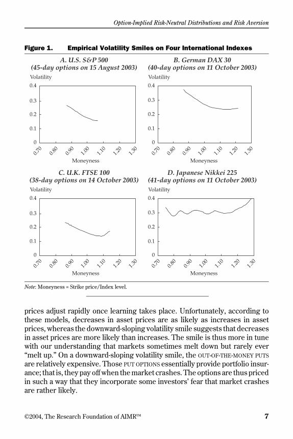
Consider a simple economy in which the stock can evolve into one of onlytwo states in the future—in this case, in one year (i.e., the stock price evolutionis modeled as a one-step BINOMIAL TREE). The current stock price is 1. In theup state, the stock price is 1.2214, and in the down state, it is 0.8187. The actualprobabilities of the two states are 0.9 and 0.1, respectively. The bond is pricedat 1 today and has a price of 1.1 in either of the two future states. This economyis depicted in Figure 2.
If we now want to value an AT-THE-MONEY CALL on the stock—that is, a callwith a strike price of 1—we can naively calculate the discounted expected
Option-Implied Risk-Neutral Distributions and Risk Aversion
10 ©2004, The Research Foundation of AIMR™
payoff (= max of 0 and the stock price minus the strike price) under the actualprobabilities. The payoff in the up state is 0.2214, and in the down state, it is 0.The expected payoff is, therefore, 0.9 × 0.2214 + (0.1 × 0) = 0.1993. The bondprices imply a risk-free rate of 10 percent, so the discounted expected payoffof the call is 0.1993/1.1 = 0.1811. The true price of the call, however, is only0.1406.
The reason for the difference is that investors receive the payoff from thecall in the up state when they are already wealthy. In that state, they have lessappreciation for additional cash flows and will accordingly pay less for the call.Therefore, to work out the true price of the call, we must turn to the conceptof STATE PRICES. The up-state price is what an investor is willing to pay for thecertain payment of 1.00 in the up state, and similarly, the down state has a stateprice. With the two existing securities, the stock and the bond, and two stateprices, πu and πd, we have a so-called complete market (one with the samenumber of states as securities and with linearly independent payoffs) and canset up a system of equations as follows: For the stock,
1 = πu1.2214 + πd0.8187, (3a)
and for the bond,
1 = πu1.1000 + πd1.1000. (3b)
Equation 3a says that the stock is worth its payoff in the up state, valuedwith the state price that we are paying for receiving 1.00 in that state, plus itspayoff in the down state, valued at the state price that we are paying forreceiving 1.00 in that state. The second equation values the bond. The solu-tions to this system of equations are πu = 0.6350 and πd = 0.2741.
Figure 2. Simple One-Period, Two-State Economy
Stock
Bond
1
1
1.2214
0.8187
1.10000.9
0.1
0.9
0.1
1.1000
Option-Implied Risk-Neutral Distributions and Risk Aversion
©2004, The Research Foundation of AIMR™ 11
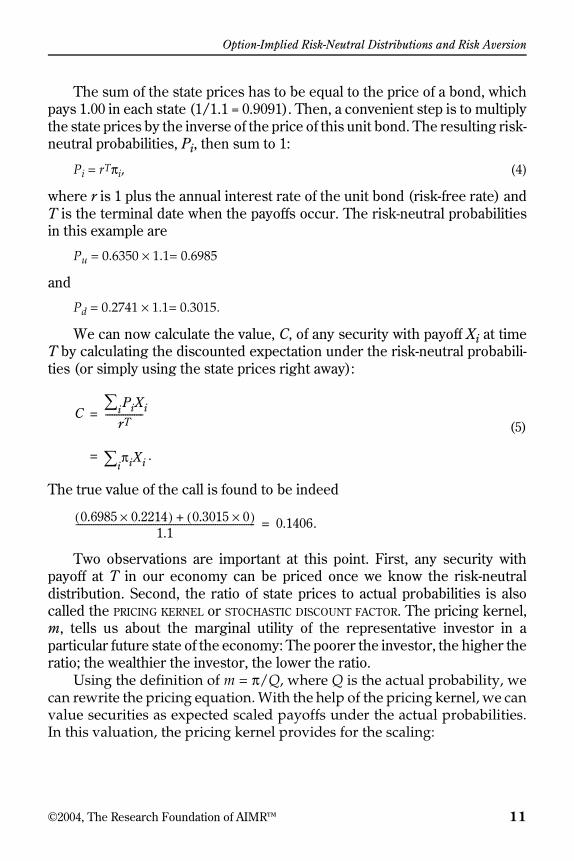
The sum of the state prices has to be equal to the price of a bond, whichpays 1.00 in each state (1/1.1 = 0.9091). Then, a convenient step is to multiplythe state prices by the inverse of the price of this unit bond. The resulting risk-neutral probabilities, Pi, then sum to 1:
Pi = rTπi, (4)
where r is 1 plus the annual interest rate of the unit bond (risk-free rate) andT is the terminal date when the payoffs occur. The risk-neutral probabilitiesin this example are
Pu = 0.6350 × 1.1= 0.6985
and
Pd = 0.2741 × 1.1= 0.3015.
We can now calculate the value, C, of any security with payoff Xi at timeT by calculating the discounted expectation under the risk-neutral probabili-ties (or simply using the state prices right away):
(5)
The true value of the call is found to be indeed
Two observations are important at this point. First, any security withpayoff at T in our economy can be priced once we know the risk-neutraldistribution. Second, the ratio of state prices to actual probabilities is alsocalled the PRICING KERNEL or STOCHASTIC DISCOUNT FACTOR. The pricing kernel,m, tells us about the marginal utility of the representative investor in aparticular future state of the economy: The poorer the investor, the higher theratio; the wealthier the investor, the lower the ratio.
Using the definition of m = π/Q, where Q is the actual probability, wecan rewrite the pricing equation. With the help of the pricing kernel, we canvalue securities as expected scaled payoffs under the actual probabilities.In this valuation, the pricing kernel provides for the scaling:
CPiXii∑
rT-----------------=
πiXi .i∑=
0.6985 0.2214×( ) 0.3015 0×( )+1.1
--------------------------------------------------------------------------------- 0.1406.=

Option-Implied Risk-Neutral Distributions and Risk Aversion
12 ©2004, The Research Foundation of AIMR™
(6)
In the example, the pricing kernel is
in the down state
and
in the up state.
Thus, when the investor is poor, he or she treats 1.00 received as if it happenedwith about three times the likelihood that it really did happen. When theinvestor is rich, he or she treats 1.00 received as if it happened with only aboutthree-quarters of the likelihood that it really did. Such an investor is risk aversebecause he or she does not like exposure to the down state at all and is willingto pay to avoid it. For a risk-averse investor, the pricing kernel is decreasing inwealth, as is the case here (2.7 in the down state and 0.71 in the up state).
Consider now the recovery of risk-neutral probabilities from option prices,after which we will return to the concept of marginal utility and the associatedpricing kernel puzzle.
Complete Markets. Complete markets are markets with exactly asmany securities (with linearly independent payoffs) as possible future states.The preceding example had such a market with two states and two securities.If the security prices in a complete market do not exhibit arbitrage opportuni-ties (that is, an investor cannot make money for sure and there is no riskless“free lunch”), then one can always recover a unique set of risk-neutral proba-bilities. Ross (1976) was one of the first researchers to investigate suchcomplete markets when he focused on the special case of a market with acomplete set of EUROPEAN OPTIONS, one for each state. Closely related is theresult presented by Breeden and Litzenberger (1978) that concerned the caseof a continuum of call options, so that the option prices can be expressed as afunction C(K) across strike prices K. Breeden and Litzenberger went on toderive an exact formula for the state prices as a function of future stock prices.The state price for the state in which stock price S is equal to a strike price K
CPiXii
∑rT
-------------------⎝ ⎠⎜ ⎟⎜ ⎟⎛ ⎞
=
QiQi------πiXii
∑=
QimiXi .i
∑=
0.27410.1
---------------- 2.7410=
0.63500.9
---------------- 0.7056=
Option-Implied Risk-Neutral Distributions and Risk Aversion
©2004, The Research Foundation of AIMR™ 13
then obtains as the second derivative of the call price function (if we use forwardcall prices, we obtain the risk-neutral probability distribution right away):
(7)
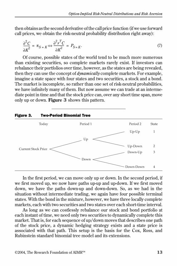
Of course, possible states of the world tend to be much more numerousthan existing securities, so complete markets rarely exist. If investors canrebalance their portfolios over time, however, as the states are being revealed,then they can use the concept of dynamically complete markets. For example,imagine a state space with four states and two securities, a stock and a bond.The market is incomplete, so rather than one set of risk-neutral probabilities,we have infinitely many of them. But now assume we can trade at an interme-diate point in time and that the stock price can, over any short time span, moveonly up or down. Figure 3 shows this pattern.
In the first period, we can move only up or down. In the second period, ifwe first moved up, we now have paths up-up and up-down. If we first moveddown, we have the paths down-up and down-down. So, as we had in thesituation without intermediate trading, we again have four possible terminalstates. With the bond in the mixture, however, we have three locally completemarkets, each with two securities and two states over each short-time interval.
As long as we can costlessly rebalance our stock and bond portfolio ateach instant of time, we need only two securities to dynamically complete thismarket. That is, for each sequence of up/down moves that describes one pathof the stock price, a dynamic hedging strategy exists and a state price isassociated with that path. This setup is the basis for the Cox, Ross, andRubinstein standard binomial tree model and its extensions.
Figure 3. Two-Period Binomial Tree
∂2C
∂K2---------- πS K=
∂2rTC
∂K2---------------⇔ PS K= .= =
Up-Up
Up
Current Stock Price
Down
Up-Down
Down-Up
Down-Down
Today Period 1 Period 2
1
2
3
4
State
Option-Implied Risk-Neutral Distributions and Risk Aversion
14 ©2004, The Research Foundation of AIMR™
Still, most markets are not even dynamically complete. Thus, we face theproblem of recovering the risk-neutral distribution in incomplete markets.
Incomplete Markets. Incomplete markets exist for many reasons. Posi-tion limits and short-sale restrictions can lead to incomplete markets, as cantrading costs. The asset price may be driven by additional stochastic factors—such as stochastic volatility, stochastic interest rates, or stochastic jumps—that are not traded. In all of these cases, an investor cannot exactly replicatethe payoff of an option state by state. In terms of risk-neutral probabilitydistributions, the result is multiple risk-neutral distributions, all of which canprice all existing assets correctly. Pricing a new security—one that is currentlynot being traded (a call option)—with these multiple risk-neutral distributionswill yield a range of option prices between a lower and an upper bound.
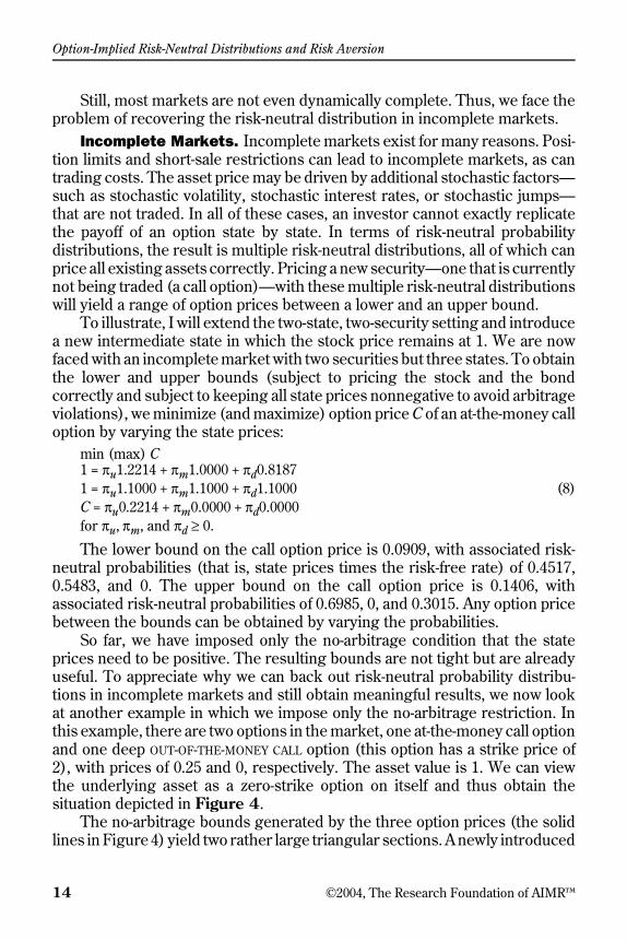
To illustrate, I will extend the two-state, two-security setting and introducea new intermediate state in which the stock price remains at 1. We are nowfaced with an incomplete market with two securities but three states. To obtainthe lower and upper bounds (subject to pricing the stock and the bondcorrectly and subject to keeping all state prices nonnegative to avoid arbitrageviolations), we minimize (and maximize) option price C of an at-the-money calloption by varying the state prices:
min (max) C1 = πu1.2214 + πm1.0000 + πd0.81871 = πu1.1000 + πm1.1000 + πd1.1000 (8)C = πu0.2214 + πm0.0000 + πd0.0000for πu, πm, and πd ≥ 0.
The lower bound on the call option price is 0.0909, with associated risk-neutral probabilities (that is, state prices times the risk-free rate) of 0.4517,0.5483, and 0. The upper bound on the call option price is 0.1406, withassociated risk-neutral probabilities of 0.6985, 0, and 0.3015. Any option pricebetween the bounds can be obtained by varying the probabilities.
So far, we have imposed only the no-arbitrage condition that the stateprices need to be positive. The resulting bounds are not tight but are alreadyuseful. To appreciate why we can back out risk-neutral probability distribu-tions in incomplete markets and still obtain meaningful results, we now lookat another example in which we impose only the no-arbitrage restriction. Inthis example, there are two options in the market, one at-the-money call optionand one deep OUT-OF-THE-MONEY CALL option (this option has a strike price of2), with prices of 0.25 and 0, respectively. The asset value is 1. We can viewthe underlying asset as a zero-strike option on itself and thus obtain thesituation depicted in Figure 4.
The no-arbitrage bounds generated by the three option prices (the solidlines in Figure 4) yield two rather large triangular sections. A newly introduced

Option-Implied Risk-Neutral Distributions and Risk Aversion
©2004, The Research Foundation of AIMR™ 15
option price would have to lie in either of those triangles to not violate the no-arbitrage condition. The resulting bounds on option prices based on only thesethree prices are so wide that they are virtually useless in real markets, but realmarket situations do often present 10 or more option prices close to at themoney, which significantly tightens the bounds.
To improve these bounds, we call on the Breeden–Litzenberger resultthat the state price density is the second derivative of a convex call pricefunction that must go through our three existing option prices. To obtainreasonable risk-neutral distributions, our call price functions themselves needto be fairly smooth. Two such candidate call price functions are plotted as thedotted lines in Figure 4. The possible locations for such smooth call pricefunctions are much more limited than the no-arbitrage bounds. Thus, as longas we require that the risk-neutral distributions be not too erratic, we canobtain significantly tighter bounds on option prices.
The proposed additional restriction here (smoothness of the call pricefunction or, equivalently, of the pricing kernel) is a novel suggestion. Otherrestrictions have been proposed in the literature. Perrakis (1986) and Ritch-ken (1985) were among the first to suggest that, in addition to keeping thestate prices (or the pricing kernel) positive, one should also (to be consistentwith risk-averse investors) require the pricing kernel to be monotonicallydecreasing in wealth. Violation of these bounds implies that risk-averse inves-tors with increasing and concave utility of wealth can increase their utility bytrading in the index, the risk-free rate, and the option in violation of the bounds.
Figure 4. No-Arbitrage Bounds on Option Prices
Note: All shaded areas represent arbitrage violation. Strike price/Index level = Moneyness.
Normalized Call Option Price
1.00
0.75
0.50
0.25
00 2.00.5 1.0 1.5
Strike Price/Index Level

Option-Implied Risk-Neutral Distributions and Risk Aversion
16 ©2004, The Research Foundation of AIMR™
Empirically, these bounds are not often violated because they are still notparticularly tight; even the steep index volatility smile fits within the boundsmost of the time.
Tightening these bounds by introducing more restrictions (and giving upthe restriction on the monotonically decreasing pricing kernel), Bernardo andLedoit (2000) and Cochrane and Saa-Requejo (2000) derived bounds on optionprices through limits on the profitability of investments. Bernardo and Ledoitargued that restrictions should be put on the ratio of expected gains toexpected losses, which limits how far the pricing kernel can deviate from areference pricing kernel. The choice of this reference pricing kernel is a majorproblem because researchers do not agree on what the reference investor,whose pricing kernel is to be used, should be like. Cochrane and Saa-Requejoargued that the SHARPE RATIO (that is, expected excess return per unit ofvolatility) should be limited, a restriction that can be expressed in terms of alimit on the variability (variance) of the pricing kernel. This argument makessense in equilibrium because extremely profitable opportunities should notexist in competitive markets (just as a free lunch as a result of arbitrage profitsshould not exist in equilibrium). Unfortunately, although Cochrane and Saa-Requejo could tighten the no-arbitrage bounds in some places, in others, theycould achieve only the no-arbitrage bounds that we have already judged to betoo loose.
Masson and Perrakis (2000) analyzed bounds on option prices when theunderlying stochastic process includes a stochastic jump component. Animportant step toward increasing realism in a model is to derive bounds thatallow intermediate trading (as opposed to buy-and-hold bounds). Constan-tinides and Perrakis (2002) provided such bounds, and empirical tests on S&P500 options have shown that they are much tighter than existing bounds.Many more index options violated these bounds than violated the one-periodbounds of Perrakis and of Ritchken. In another version of the Constantinides–Perrakis bounds, transaction costs caused the bounds to widen again whenthe investor had to pay transaction costs at each intermediate trading date.Nevertheless, we will find in the section “Implied Risk Aversion” some evi-dence that even static buy-and-hold strategies can earn abnormal profits in theindex market when the volatility smile seems to be too steep.
The Inverse ProblemKnowledge of the risk-neutral probability distribution is desirable because itallows us to price any derivative of the particular underlying asset with thesame time to expiration. Moreover, we can learn about the actual probabilities(for forecasting purposes) from the risk-neutral probability distributionthrough the link of the economywide scaled marginal utility (the pricing
Option-Implied Risk-Neutral Distributions and Risk Aversion
©2004, The Research Foundation of AIMR™ 17
kernel). As a result, several methods have been developed to back out therisk-neutral probability distributions from option prices.
In this section, we investigate these approaches and their characteristics.The approaches selected are either particularly stable or easy to implementor both. Because all the existing models have some drawback, however, Ipropose a new and particularly simple algorithm that can be used for actualwork. We then examine studies that have used risk-neutral distributions forforecasting and economic analysis. Finally, we turn to a practical question:How can investment professionals use these distributions to their advantage?
Because of the paucity of option prices in the 1970s and 1980s, not muchempirical research was conducted at that time, so the history of recoveringoption-implied risk-neutral distributions is short. Banz and Miller (1978)highlight this problem. For purposes of capital budgeting, they backed risk-neutral probabilities out of a set of option prices, but in their example, theysimply used hypothetical Black–Scholes-based option prices. As a result, theybacked out the associated lognormal probabilities.
The next attempt to derive a histogram of risk-neutral probabilities fromoption prices was made by Longstaff (1990), who distributed the risk-neutralprobability uniformly between any two adjacent strike prices. His methodturned out to be numerically unstable, however, and yielded risk-neutraldistributions for which the probabilities oscillated between large positive andlarge negative values. Mayhew investigated this problem and showed that thecause was the coarseness of the options data, which was observable only atdiscrete strikes. S&P 500 options have strike prices that differ by multiples of$5.00.
In the mid-1990s, research picked up as large options databases andpowerful computers became available. In particular, the CBOE made thecomplete tick-by-tick options record from the early 1980s to 1995 availablethrough the Berkeley Options Database. Unfortunately, the board stoppedproviding these valuable data at the end of 1995 and prohibited further sale ofany of the data. Also, a number of research papers (e.g., Rubinstein 1994;Derman and Kani 1994) provided the theoretical background needed for theexplosion in methods to recover the risk-neutral distribution.
From the multitude of these methods, we can discern two basicapproaches: One is parametric, and the other is nonparametric. They have incommon that the models of option prices developed in them depend on somenumber of variables that are moved around until they “best fit” the observedoption prices.6 Parametric approaches specify their models as functions of a
6As discussed later, “best” was defined in various ways—lowest absolute pricing error, lowestaverage error, and so on.

Option-Implied Risk-Neutral Distributions and Risk Aversion
18 ©2004, The Research Foundation of AIMR™
few (often, four) variables, whereas nonparametric models use many variables(usually 50 to 200 but up to 1,000 at times). The benefit of nonparametricmodels is the superior fit of option prices; the cost is unwieldy models thatoscillate widely from one date to the next. The fluctuations are the result ofoverfitting, when small changes in market prices arising from noise in the dataare fitted by the model.
Four articles are available to the reader who wants a deeper understand-ing of these methods—Cont (1997), Bahra (1997), Jackwerth (1999), andPerignon and Villa (2002). Cont focused on methods for obtaining the risk-neutral distributions, whereas the other surveys also covered applications. Inthis section, I follow a structure similar to that of Cont’s and Jackwerth’s; wewill explore parametric methods first and nonparametric methods second.
Parametric Methods. In the simple parametric case, we pick a trial setof parameters for our risk-neutral probability distribution (e.g., a two-param-eter lognormal distribution with known mean and volatility), price all optionsbased on this distribution, and vary the parameters of the distribution tominimize the pricing error. This method has drawbacks if we use a parametricprobability distribution that is not flexible enough for matching the observedoption prices. As we have seen, the two-parameter lognormal distribution (onwhich the Black–Scholes model is based) is not sufficiently flexible to fitobserved (index) option prices.
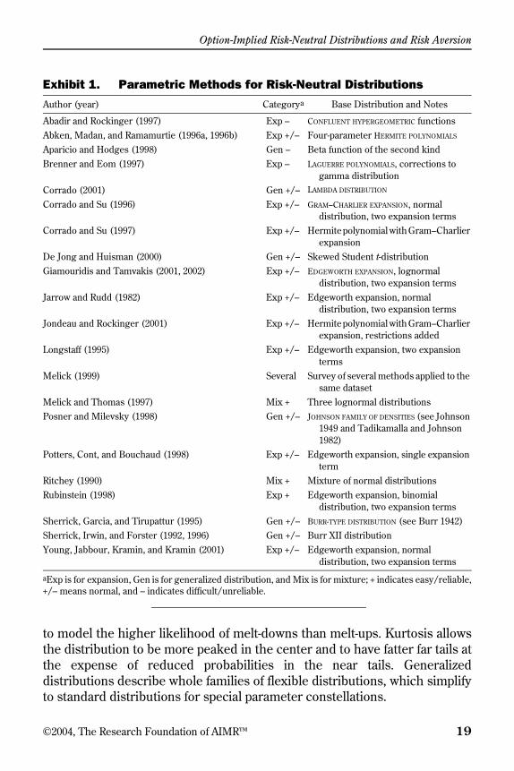
The specific models are categorized in Exhibit 1.7 Within the parametricmethods, we can identify three groups—expansion methods, generalizeddistribution methods, and mixture methods.
■ Expansion methods. Expansion methods start with a simple knownprobability distribution (often normal or lognormal) and then add correctionterms to it. Expansion methods are conceptually related to Taylor seriesexpansions for simple functions. These correction terms are often notguaranteed to preserve the integrity of the probability distribution, so the usermust always check that the resulting distribution is strictly positive andintegrates to 1.
■ Generalized distribution methods. Generalized distribution methodsuse distribution functions with more than the typical two parameters for themean and the volatility; they often add SKEWNESS and KURTOSIS parameters.Skewness allows the (left) tail of the distribution to be fatter than the right tail
7Further detail is found in the references, but I strongly suggest using the nonparametricmethod described in the next section because it avoids the problems that afflict theseparametric models.
Option-Implied Risk-Neutral Distributions and Risk Aversion
©2004, The Research Foundation of AIMR™ 19
to model the higher likelihood of melt-downs than melt-ups. Kurtosis allowsthe distribution to be more peaked in the center and to have fatter far tails atthe expense of reduced probabilities in the near tails. Generalizeddistributions describe whole families of flexible distributions, which simplifyto standard distributions for special parameter constellations.
Exhibit 1. Parametric Methods for Risk-Neutral Distributions
Author (year) Categorya Base Distribution and Notes
Abadir and Rockinger (1997) Exp – CONFLUENT HYPERGEOMETRIC functionsAbken, Madan, and Ramamurtie (1996a, 1996b) Exp +/– Four-parameter HERMITE POLYNOMIALS
Aparicio and Hodges (1998) Gen – Beta function of the second kindBrenner and Eom (1997) Exp – LAGUERRE POLYNOMIALS, corrections to
gamma distributionCorrado (2001) Gen +/– LAMBDA DISTRIBUTION
Corrado and Su (1996) Exp +/– GRAM–CHARLIER EXPANSION, normal distribution, two expansion terms
Corrado and Su (1997) Exp +/– Hermite polynomial with Gram–Charlier expansion
De Jong and Huisman (2000) Gen +/– Skewed Student t-distributionGiamouridis and Tamvakis (2001, 2002) Exp +/– EDGEWORTH EXPANSION, lognormal
distribution, two expansion termsJarrow and Rudd (1982) Exp +/– Edgeworth expansion, normal
distribution, two expansion termsJondeau and Rockinger (2001) Exp +/– Hermite polynomial with Gram–Charlier
expansion, restrictions addedLongstaff (1995) Exp +/– Edgeworth expansion, two expansion
termsMelick (1999) Several Survey of several methods applied to the
same datasetMelick and Thomas (1997) Mix + Three lognormal distributionsPosner and Milevsky (1998) Gen +/– JOHNSON FAMILY OF DENSITIES (see Johnson
1949 and Tadikamalla and Johnson 1982)
Potters, Cont, and Bouchaud (1998) Exp +/– Edgeworth expansion, single expansion term
Ritchey (1990) Mix + Mixture of normal distributionsRubinstein (1998) Exp + Edgeworth expansion, binomial
distribution, two expansion termsSherrick, Garcia, and Tirupattur (1995) Gen +/– BURR-TYPE DISTRIBUTION (see Burr 1942)Sherrick, Irwin, and Forster (1992, 1996) Gen +/– Burr XII distributionYoung, Jabbour, Kramin, and Kramin (2001) Exp +/– Edgeworth expansion, normal
distribution, two expansion terms
aExp is for expansion, Gen is for generalized distribution, and Mix is for mixture; + indicates easy/reliable,+/– means normal, and – indicates difficult/unreliable.
Option-Implied Risk-Neutral Distributions and Risk Aversion
20 ©2004, The Research Foundation of AIMR™
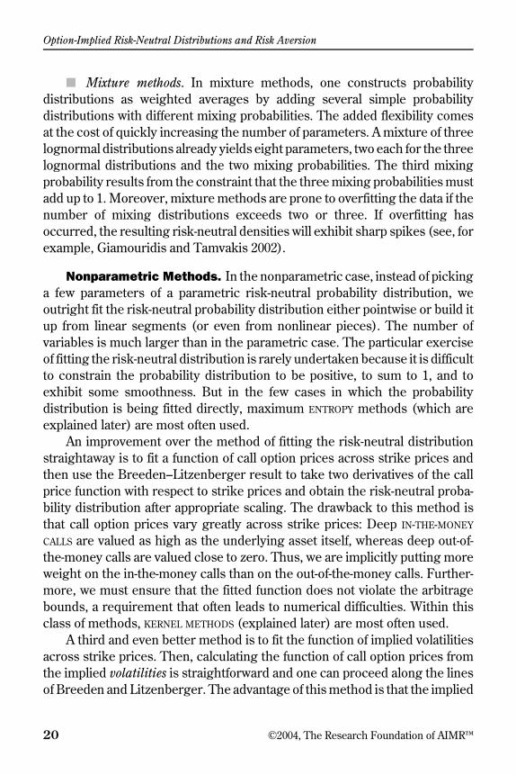
■ Mixture methods. In mixture methods, one constructs probabilitydistributions as weighted averages by adding several simple probabilitydistributions with different mixing probabilities. The added flexibility comesat the cost of quickly increasing the number of parameters. A mixture of threelognormal distributions already yields eight parameters, two each for the threelognormal distributions and the two mixing probabilities. The third mixingprobability results from the constraint that the three mixing probabilities mustadd up to 1. Moreover, mixture methods are prone to overfitting the data if thenumber of mixing distributions exceeds two or three. If overfitting hasoccurred, the resulting risk-neutral densities will exhibit sharp spikes (see, forexample, Giamouridis and Tamvakis 2002).
Nonparametric Methods. In the nonparametric case, instead of pickinga few parameters of a parametric risk-neutral probability distribution, weoutright fit the risk-neutral probability distribution either pointwise or build itup from linear segments (or even from nonlinear pieces). The number ofvariables is much larger than in the parametric case. The particular exerciseof fitting the risk-neutral distribution is rarely undertaken because it is difficultto constrain the probability distribution to be positive, to sum to 1, and toexhibit some smoothness. But in the few cases in which the probabilitydistribution is being fitted directly, maximum ENTROPY methods (which areexplained later) are most often used.
An improvement over the method of fitting the risk-neutral distributionstraightaway is to fit a function of call option prices across strike prices andthen use the Breeden–Litzenberger result to take two derivatives of the callprice function with respect to strike prices and obtain the risk-neutral proba-bility distribution after appropriate scaling. The drawback to this method isthat call option prices vary greatly across strike prices: Deep IN-THE-MONEY
CALLS are valued as high as the underlying asset itself, whereas deep out-of-the-money calls are valued close to zero. Thus, we are implicitly putting moreweight on the in-the-money calls than on the out-of-the-money calls. Further-more, we must ensure that the fitted function does not violate the arbitragebounds, a requirement that often leads to numerical difficulties. Within thisclass of methods, KERNEL METHODS (explained later) are most often used.
A third and even better method is to fit the function of implied volatilitiesacross strike prices. Then, calculating the function of call option prices fromthe implied volatilities is straightforward and one can proceed along the linesof Breeden and Litzenberger. The advantage of this method is that the implied
Option-Implied Risk-Neutral Distributions and Risk Aversion
©2004, The Research Foundation of AIMR™ 21
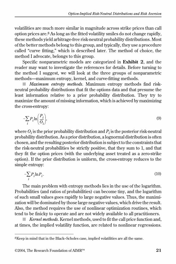
volatilities are much more similar in magnitude across strike prices than calloption prices are.8 As long as the fitted volatility smiles do not change rapidly,these methods yield arbitrage-free risk-neutral probability distributions. Mostof the better methods belong to this group, and typically, they use a procedurecalled “curve fitting,” which is described later. The method of choice, themethod I advocate, belongs to this group.
Specific nonparametric models are categorized in Exhibit 2, and thereader may want to investigate the references for details. Before turning tothe method I suggest, we will look at the three groups of nonparametricmethods—maximum entropy, kernel, and curve-fitting methods.
■ Maximum entropy methods. Maximum entropy methods find risk-neutral probability distributions that fit the options data and that presume theleast information relative to a prior probability distribution. They try tomaximize the amount of missing information, which is achieved by maximizingthe cross-entropy:
(9)
where Oi is the prior probability distribution and Pi is the posterior risk-neutralprobability distribution. As a prior distribution, a lognormal distribution is oftenchosen, and the resulting posterior distribution is subject to the constraints thatthe risk-neutral probabilities be strictly positive, that they sum to 1, and thatthey fit the option prices (with the underlying asset treated as a zero-strikeoption). If the prior distribution is uniform, the cross-entropy reduces to thesimple entropy:
(10)
The main problem with entropy methods lies in the use of the logarithm.Probabilities (and ratios of probabilities) can become tiny, and the logarithmof such small values goes rapidly to large negative values. Thus, the maximi-zation will be dominated by those large negative values, which drive the result.Also, the method requires the use of nonlinear optimization routines, whichtend to be finicky to operate and are not widely available to all practitioners.
■ Kernel methods. Kernel methods, used to fit the call price function and,at times, the implied volatility function, are related to nonlinear regressions.
8Keep in mind that in the Black–Scholes case, implied volatilities are all the same.
PiPiOi------⎝ ⎠⎜ ⎟⎛ ⎞
ln ,i∑–
Pi Piln .i∑–

Option-Implied Risk-Neutral Distributions and Risk Aversion
22 ©2004, The Research Foundation of AIMR™
They do not specify the linear form of a standard regression. Instead, they arelocalized. They start from the concept that each data point suggests the centerof a region through which the function passes. The function is assumed topass most likely right through the data point, and a kernel, k(x), measures thelikelihood that the function passes by the data point at a distance. A typicalkernel is the standard normal distribution whichmeasures the drop in likelihood of being further away from a data point.
Exhibit 2. Nonparametric Methods for Risk-Neutral Distributions
Author (year) Categorya Description and Notes
Aït-Sahalia and Lo (1998) Ker + Kernel estimator in stock price, strike, maturity, interest rate, and dividends
Andersen and Wagener (2002) Cur +/– Higher-order splines fitted to implied volatilitiesAparicio and Hodges (1998) Cur +/– Cubic B-splines fitted to implied volatilitiesBondarenko (2000) Ker +/– Convolution of kernel and standard densitiesBranger (2002) Max +/– Maximum entropyBrown and Toft (1999) Cur +/– Seventh-order splines fitted to implied volatilitiesBuchen and Kelly (1996) Max +/– Maximum entropy with uniform and lognormal priorsCampa, Chang, and Reider (1998) Cur +/– Cubic splines fitted to implied volatilitiesHärdle and Yatchew (2002) Ker – Nonparametric least squares through option pricesHartvig, Jensen, and Pedersen (1999) Cur +/– Piecewise linear fit of log of the risk-neutral probability
distributionHayes and Shin (2002) Cur +/– Cubic splines fitted to implied volatilities across deltasJackwerth (2000) Cur + Maximizing the smoothness of pointwise implied
volatilitiesMalz (1997) Cur + Quadratic polynomials fitted to implied volatilities
across deltasMayhew (1995) Cur +/– Cubic splines fitted to implied volatilitiesPritsker (1998) Ker + Kernel estimatorRockinger and Jondeau (2002) Max +/– Maximum entropy with normal, t, and generalized
error distribution priors, added restrictionsRookley (1997) Ker + Bivariate kernel in moneyness and time to expirationRosenberg (1998, 2003) Cur + Bivariate polynomial fitted to log implied volatilitiesRosenberg and Engle (2002) Cur + Polynomial fitted to log implied volatilitiesRubinstein (1994) Max +/– Maximum entropy with lognormal priorRubinstein (1994) Cur + Minimum distance between discrete and lognormal
distributionShimko (1993) Cur + Quadratic polynomial fitted to implied volatilitiesStutzer (1996) Max +/– Maximum entropy with historical distribution as prior
aKer is for kernel, Max is for maximum entropy, and Cur is for curve fitting; + indicates easy/reliable, +/–means normal, and – indicates difficult/unreliable.
n x( ) 1 2π⁄⎝ ⎠⎛ ⎞ e 0.5x2
– ,=
Option-Implied Risk-Neutral Distributions and Risk Aversion
©2004, The Research Foundation of AIMR™ 23
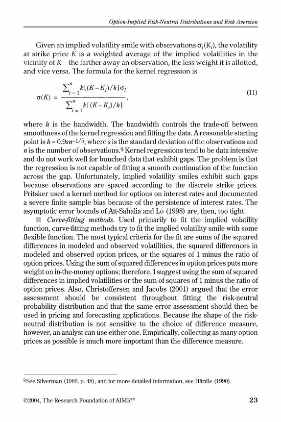
Given an implied volatility smile with observations σi(Ki), the volatilityat strike price K is a weighted average of the implied volatilities in thevicinity of K—the farther away an observation, the less weight it is allotted,and vice versa. The formula for the kernel regression is
(11)
where h is the bandwidth. The bandwidth controls the trade-off betweensmoothness of the kernel regression and fitting the data. A reasonable startingpoint is h = 0.9sn–1/5, where s is the standard deviation of the observations andn is the number of observations.9 Kernel regressions tend to be data intensiveand do not work well for bunched data that exhibit gaps. The problem is thatthe regression is not capable of fitting a smooth continuation of the functionacross the gap. Unfortunately, implied volatility smiles exhibit such gapsbecause observations are spaced according to the discrete strike prices.Pritsker used a kernel method for options on interest rates and documenteda severe finite sample bias because of the persistence of interest rates. Theasymptotic error bounds of Aït-Sahalia and Lo (1998) are, then, too tight.
■ Curve-fitting methods. Used primarily to fit the implied volatilityfunction, curve-fitting methods try to fit the implied volatility smile with someflexible function. The most typical criteria for the fit are sums of the squareddifferences in modeled and observed volatilities, the squared differences inmodeled and observed option prices, or the squares of 1 minus the ratio ofoption prices. Using the sum of squared differences in option prices puts moreweight on in-the-money options; therefore, I suggest using the sum of squareddifferences in implied volatilities or the sum of squares of 1 minus the ratio ofoption prices. Also, Christoffersen and Jacobs (2001) argued that the errorassessment should be consistent throughout fitting the risk-neutralprobability distribution and that the same error assessment should then beused in pricing and forecasting applications. Because the shape of the risk-neutral distribution is not sensitive to the choice of difference measure,however, an analyst can use either one. Empirically, collecting as many optionprices as possible is much more important than the difference measure.
9See Silverman (1986, p. 48), and for more detailed information, see Härdle (1990).
σ K( )k[ K Ki–( )/h]σii 1=
n∑
k[(K Ki– )/h]i 1=
n∑----------------------------------------------------------- ,=
Option-Implied Risk-Neutral Distributions and Risk Aversion
24 ©2004, The Research Foundation of AIMR™
Typical functions for curve fitting are polynomials in the strike price[σ(K) = α0 + α1K + α2K2 + . . . + αnKn], but they can exhibit oscillatorybehavior if they involve higher-order terms. Here, SPLINES are a better choice;splines piece together polynomial segments at so-called knots by matchinglevels and derivatives at the knots. The choice of the location of those knotsis somewhat of an art; too many knots cause overfitting of the data and toofew knots prevent the observed volatilities from being matched. Splinestend to be smoother and do not exhibit the oscillations that polynomials areprone to, but they need to be of an order higher than 3 for the probabilitydistribution to turn out to be smooth.
Shimko first proposed fitting a quadratic polynomial to the impliedvolatilities. He translated those implied volatilities into call option pricesand then obtained the risk-neutral distribution through the Breeden–Litzenberger method. Because the tails contained no options data, he addedlognormal tails to the risk-neutral distribution. Malz (1997) devised a vari-ation of this method by fitting quadratic polynomials to implied volatilitiesacross call OPTION DELTAS (that is, derivatives of call option prices with respectto the stock price) instead of strike prices. Numerically, the advantage ofthis method is that the range of feasible deltas is bounded by 0 and 1,whereas the strike price range is 0 to ∞. Translating from delta space,however, back to strike prices is cumbersome. In addition, taking therequired two derivatives of the call options prices is much easier and morestable if one uses strike prices rather than deltas.
Alternatively, an analyst can explicitly fit smooth functions by penalizingjaggedness. One way is to add into the objective function a term based on thesum or integral of squared second derivatives of the function. The morecurvature the function has, the larger this term will be. A trade-off parametergoverns how much weight is given to fit versus smoothness. Its value istypically based on trial and error.
Nonparametric Methods Compared. The easiest and most stablemethods tend to be in the group of methods for curve-fitting the impliedvolatility smile. The limiting case of a flat implied volatility function simplygives the Black–Scholes model. These methods tend to be exceedingly fastand some of them require only a single calculation. As long as the impliedvolatility smile is reasonably smooth, the associated risk-neutral probabilitydistribution will be strictly positive. Because this condition is not guaranteed,however, it should be checked separately. Clark (2002) derived conditionsunder which the risk-neutral distribution will be arbitrage free, but they areeven more complicated than simple checks for positivity. The new methodthat I will propose for fast and easy computation belongs to this group.
Option-Implied Risk-Neutral Distributions and Risk Aversion
©2004, The Research Foundation of AIMR™ 25
In the meantime, I argue that, given a reasonable number of observedoptions, the choice of method does not matter much, so the analyst might aswell pick a particularly easy method. As mentioned, the risk-neutral probabil-ity distributions are limited by the no-arbitrage bounds on option prices. Thebounds on an individual option are wide—the lower bound being the intrinsicvalue of the stock and the upper bound being the stock price itself. When weconsider the no-arbitrage bounds on the sets of 10–15 option prices that aretypically traded at the same time in a liquid options market, however, thebounds turn out to be much tighter. In turn, most methods will yield similarrisk-neutral probability distributions, particularly in the center of the distribu-tion, where many option prices lie. Because less information about the tails ofthe distributions is contained in the observed option prices, the methods tendto differ in the tails.
Empirically, this point was argued by Jackwerth and Rubinstein (1996),who decided to use five measures of the distance between the prior distributionand the risk-neutral distribution, and by Campa, Chang, and Reider, who cameto a similar conclusion. They used cubic splines fitted to implied volatilities,Rubinstein’s (1994) sum of the squared distance between prior and risk-neutraldistributions, and mixtures of lognormal distributions. Further evidence wassupplied by Coutant, Jondeau, and Rockinger (2001), who also used threemethods—mixtures of lognormal distributions, HERMITE POLYNOMIAL expan-sions, and maximum entropy. Clews, Panigirtzoglou, and Proudman (2000)compared mixtures of two lognormals with a curve-fitting method and foundmuch lower standard deviations of summary statistics for the curve-fittingmethod, which indicates that one should avoid mixtures of distributions.
In summary, because the particular choice of method does not change theresults by much, an analyst might as well choose a fast and stable algorithm.
Fast and Stable Method. To deal with all of the problems described, Isuggest a new method that has a number of advantages: (1) The trade-offbetween fit and smoothness can be controlled externally, (2) the computationsare simple and can be done in an Excel spreadsheet, and (3) it requires nocomplicated mathematical functions or optimization routines. The formalalgorithm is described in Appendix A; here, I review an example that shouldsuffice to implement the method for any set of option prices.
Consider the following set of three option prices:

Option-Implied Risk-Neutral Distributions and Risk Aversion
26 ©2004, The Research Foundation of AIMR™
To keep the example manageable but still insightful, we limit ourselves to 11future index levels that are 0.1 apart from each other, which we choose so thatthe strike prices (0.9, 1, and 1.1) lie within the following set:
0.5, 0.6, 0.7, 0.8, 0.9, 1, 1.1, 1.2, 1.3, 1.4, and 1.5.
If our resulting probability distribution is too coarse or does not tend to 0in the tails, we can introduce half-steps (0.55, 0.65, etc.) or add values to theends (0.3, 0.4, 1.6, 1.7, etc.). We discover that the trade-off parameter, λ, equalto 0.01 will provide nice results. (Normally, one needs to use trial and error here:If the distribution goes negative or is too jagged, one reduces λ; if the fittedvolatilities do not match the observed volatilities sufficiently, one increases λ.)
Now, our first step is to generate a system of equations—one for eachfuture index level—with the entries 1, –4, 6, –4, and 1 around the diagonal and–3 and 3 as the top two values of the first column and the last two values of thelast column:
The solution of this system of equations so far is zero for each row wherewe multiply each coefficient with the corresponding fitted implied volatility,σi. But now we need to add the information concerning the observed optionsinto the fifth, sixth, and seventh rows (corresponding to strike prices 0.9, 1,and 1.1). The required multiplier is as follows: Trade-off parameter × (Numberof index levels/[Number of options × Index spacing to the fourth power]) or
Call = 1Put = 2
StockPrice
StrikePrice
Time to Expiration Interest Rate
Implied Volatility
Dividend Yield Price
1 1 0.9 1 0.05 0.250 0 0.1811 1 1.0 1 0.05 0.200 0 0.1041 1 1.1 1 0.05 0.150 0 0.040
3σ1 –4σ2 +1σ3 +0σ4 +0σ5 +0σ6 +0σ7 +0σ8 +0σ9 +0σ10 +0σ11 = 0–3σ1 +6σ2 –4σ3 +1σ4 +0σ5 +0σ6 +0σ7 +0σ8 +0σ9 +0σ10 +0σ11 = 01σ1 –4σ2 +6σ3 –4σ4 +1σ5 +0σ6 +0σ7 +0σ8 +0σ9 +0σ10 +0σ11 = 00σ1 +1σ2 –4σ3 +6σ4 –4σ5 +1σ6 +0σ7 +0σ8 +0σ9 +0σ10 +0σ11 = 00σ1 +0σ2 +1σ3 –4σ4 +6σ5 –4σ6 +1σ7 +0σ8 +0σ9 +0σ10 +0σ11 = 00σ1 +0σ2 +0σ3 +1σ4 –4σ5 +6σ6 –4σ7 +1σ8 +0σ9 +0σ10 +0σ11 = 00σ1 +0σ2 +0σ3 +0σ4 +1σ5 –4σ6 +6σ7 –4σ8 +1σ9 +0σ10 +0σ11 = 00σ1 +0σ2 +0σ3 +0σ4 +0σ5 +1σ6 –4σ7 +6σ8 –4σ9 +1σ10 +0σ11 = 00σ1 +0σ2 +0σ3 +0σ4 +0σ5 +0σ6 +1σ7 –4σ8 +6σ9 –4σ10 +1σ11 = 00σ1 +0σ2 +0σ3 +0σ4 +0σ5 +0σ6 +0σ7 +1σ8 –4σ9 +6σ10 –3σ11 = 00σ1 +0σ2 +0σ3 +0σ4 +0σ5 +0σ6 +0σ7 +0σ8 +1σ9 –4σ10 +3σ11 = 0
λJ 1+
I ∆4( )------------- 0.01
11
3 0.14( )×------------------------=
366.6666667.=
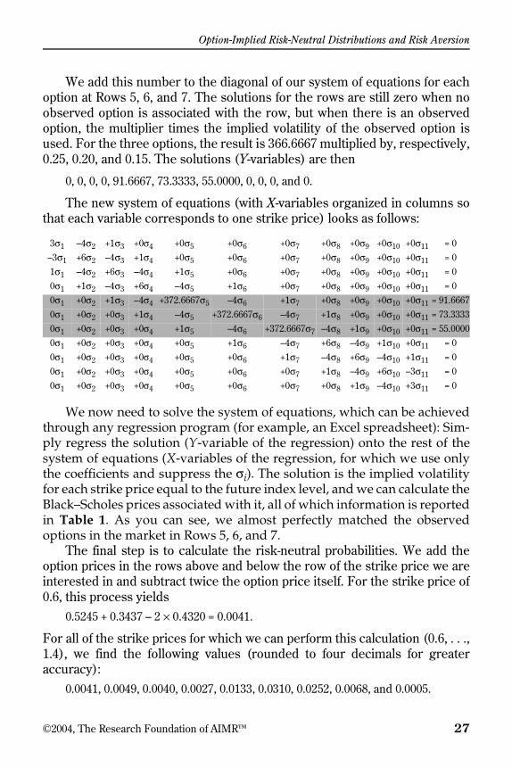
Option-Implied Risk-Neutral Distributions and Risk Aversion
©2004, The Research Foundation of AIMR™ 27
We add this number to the diagonal of our system of equations for eachoption at Rows 5, 6, and 7. The solutions for the rows are still zero when noobserved option is associated with the row, but when there is an observedoption, the multiplier times the implied volatility of the observed option isused. For the three options, the result is 366.6667 multiplied by, respectively,0.25, 0.20, and 0.15. The solutions (Y-variables) are then
0, 0, 0, 0, 91.6667, 73.3333, 55.0000, 0, 0, 0, and 0.
The new system of equations (with X-variables organized in columns sothat each variable corresponds to one strike price) looks as follows:
We now need to solve the system of equations, which can be achievedthrough any regression program (for example, an Excel spreadsheet): Sim-ply regress the solution (Y-variable of the regression) onto the rest of thesystem of equations (X-variables of the regression, for which we use onlythe coefficients and suppress the σi). The solution is the implied volatilityfor each strike price equal to the future index level, and we can calculate theBlack–Scholes prices associated with it, all of which information is reportedin Table 1. As you can see, we almost perfectly matched the observedoptions in the market in Rows 5, 6, and 7.
The final step is to calculate the risk-neutral probabilities. We add theoption prices in the rows above and below the row of the strike price we areinterested in and subtract twice the option price itself. For the strike price of0.6, this process yields
0.5245 + 0.3437 – 2 × 0.4320 = 0.0041.
For all of the strike prices for which we can perform this calculation (0.6, . . .,1.4), we find the following values (rounded to four decimals for greateraccuracy):
0.0041, 0.0049, 0.0040, 0.0027, 0.0133, 0.0310, 0.0252, 0.0068, and 0.0005.
3σ1 –4σ2 +1σ3 +0σ4 +0σ5 +0σ6 +0σ7 +0σ8 +0σ9 +0σ10 +0σ11 = 0–3σ1 +6σ2 –4σ3 +1σ4 +0σ5 +0σ6 +0σ7 +0σ8 +0σ9 +0σ10 +0σ11 = 01σ1 –4σ2 +6σ3 –4σ4 +1σ5 +0σ6 +0σ7 +0σ8 +0σ9 +0σ10 +0σ11 = 00σ1 +1σ2 –4σ3 +6σ4 –4σ5 +1σ6 +0σ7 +0σ8 +0σ9 +0σ10 +0σ11 = 00σ1 +0σ2 +1σ3 –4σ4 +372.6667σ5 –4σ6 +1σ7 +0σ8 +0σ9 +0σ10 +0σ11 = 91.66670σ1 +0σ2 +0σ3 +1σ4 –4σ5 +372.6667σ6 –4σ7 +1σ8 +0σ9 +0σ10 +0σ11 = 73.33330σ1 +0σ2 +0σ3 +0σ4 +1σ5 –4σ6 +372.6667σ7 –4σ8 +1σ9 +0σ10 +0σ11 = 55.00000σ1 +0σ2 +0σ3 +0σ4 +0σ5 +1σ6 –4σ7 +6σ8 –4σ9 +1σ10 +0σ11 = 00σ1 +0σ2 +0σ3 +0σ4 +0σ5 +0σ6 +1σ7 –4σ8 +6σ9 –4σ10 +1σ11 = 00σ1 +0σ2 +0σ3 +0σ4 +0σ5 +0σ6 +0σ7 +1σ8 –4σ9 +6σ10 –3σ11 = 00σ1 +0σ2 +0σ3 +0σ4 +0σ5 +0σ6 +0σ7 +0σ8 +1σ9 –4σ10 +3σ11 = 0
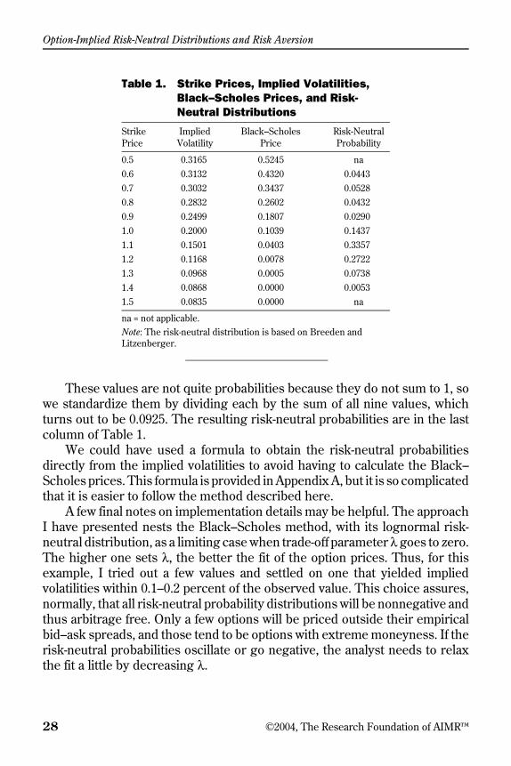
Option-Implied Risk-Neutral Distributions and Risk Aversion
28 ©2004, The Research Foundation of AIMR™
These values are not quite probabilities because they do not sum to 1, sowe standardize them by dividing each by the sum of all nine values, whichturns out to be 0.0925. The resulting risk-neutral probabilities are in the lastcolumn of Table 1.
We could have used a formula to obtain the risk-neutral probabilitiesdirectly from the implied volatilities to avoid having to calculate the Black–Scholes prices. This formula is provided in Appendix A, but it is so complicatedthat it is easier to follow the method described here.
A few final notes on implementation details may be helpful. The approachI have presented nests the Black–Scholes method, with its lognormal risk-neutral distribution, as a limiting case when trade-off parameter λ goes to zero.The higher one sets λ, the better the fit of the option prices. Thus, for thisexample, I tried out a few values and settled on one that yielded impliedvolatilities within 0.1–0.2 percent of the observed value. This choice assures,normally, that all risk-neutral probability distributions will be nonnegative andthus arbitrage free. Only a few options will be priced outside their empiricalbid–ask spreads, and those tend to be options with extreme moneyness. If therisk-neutral probabilities oscillate or go negative, the analyst needs to relaxthe fit a little by decreasing λ.
Table 1. Strike Prices, Implied Volatilities, Black–Scholes Prices, and Risk-Neutral Distributions
Strike Price
ImpliedVolatility
Black–Scholes Price
Risk-Neutral Probability
0.5 0.3165 0.5245 na0.6 0.3132 0.4320 0.04430.7 0.3032 0.3437 0.05280.8 0.2832 0.2602 0.04320.9 0.2499 0.1807 0.02901.0 0.2000 0.1039 0.14371.1 0.1501 0.0403 0.33571.2 0.1168 0.0078 0.27221.3 0.0968 0.0005 0.07381.4 0.0868 0.0000 0.00531.5 0.0835 0.0000 na
na = not applicable.Note: The risk-neutral distribution is based on Breeden and Litzenberger.

Option-Implied Risk-Neutral Distributions and Risk Aversion
©2004, The Research Foundation of AIMR™ 29
The case of AMERICAN OPTIONS presents a problem: The methods forbacking out risk-neutral distributions, including this one, strictly apply onlyto European option prices. To use American option prices, one has to eitherverify that there will be no early exercise10 or one has to approximate the earlyexercise premium and subtract it from the price of the American option. Oneway of achieving this step is to fit a standard binomial tree (Cox, Ross, andRubinstein) to the American option to obtain the implied volatility and thenuse the same binomial tree to value a hypothetical European option with thesame parameters. The estimation of the risk-neutral distributions can then bebased on the hypothetical European options. An alternative method is to usethe approximate American option-pricing formula of Barone-Adesi and Wha-ley (1987) and proceed as described here. Because Cox–Ross–Rubinstein iscorrect in the limit, not merely an approximation, I prefer that method.
Finally, here is a real-world example of application of our methodology. Ibacked out the risk-neutral distributions of four international indexes corre-sponding to the volatility smiles of Figure 1. Figure 5 provides the results.
The proposed method performed well. The shapes of the risk-neutraldistributions are what the implied volatility smiles in Figure 1 led us to expect.Because the volatility smiles are steeply downward sloping for the UnitedStates, Germany, and the United Kingdom, we would expect the risk-neutraldistributions to be left skewed and peaked in the center, just as they are inreal life. The relatively flat implied volatility smile for Japan led us to suspectthat the risk-neutral distribution would look more lognormal than the distri-bution for the other markets, and Figure 5 shows that it does.
Studies of Inverse Methods. With the risk-neutral probability distri-bution, one can price any arbitrary payoff with the same time to expiration.Normally, this method is applied to the pricing of exotic, illiquid options byfirst obtaining the risk-neutral probability distribution from plain vanillaoptions. This method then allows us to price the exotic options consistentlywith the plain vanilla options.11
An area of great interest is using the risk-neutral distribution to obtain tailprobabilities of rare (down-market) events. Such distributions could be used,for example, in value-at-risk (VAR) applications. The work of Jackwerth and
10Merton gives the exact conditions when these options will not be exercised; generally,American calls that do not pay dividends should never be exercised early.11Pricing American options is precluded because they lack a single time to expiration. ForAmerican options, we have to use either the approaches described in the preceding section orimplied binomial trees, which are described in the section “Implied Binomial Trees.” Impliedbinomial trees model the complete stochastic process between now at time t and the optionexpiration and are thus capable of pricing American or barrier options.
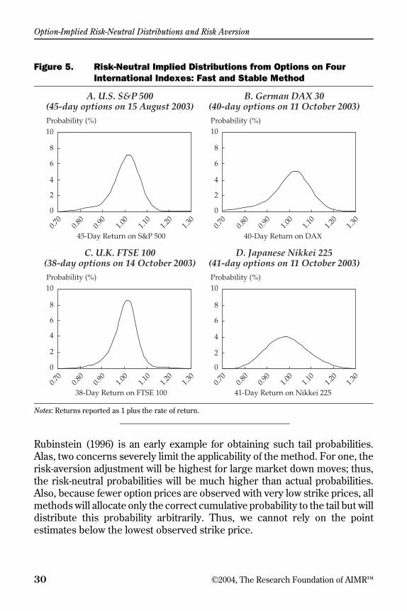
Option-Implied Risk-Neutral Distributions and Risk Aversion
30 ©2004, The Research Foundation of AIMR™
Rubinstein (1996) is an early example for obtaining such tail probabilities.Alas, two concerns severely limit the applicability of the method. For one, therisk-aversion adjustment will be highest for large market down moves; thus,the risk-neutral probabilities will be much higher than actual probabilities.Also, because fewer option prices are observed with very low strike prices, allmethods will allocate only the correct cumulative probability to the tail but willdistribute this probability arbitrarily. Thus, we cannot rely on the pointestimates below the lowest observed strike price.
Figure 5. Risk-Neutral Implied Distributions from Options on Four International Indexes: Fast and Stable Method
Notes: Returns reported as 1 plus the rate of return.
38-Day Return on FTSE 100 41-Day Return on Nikkei 225
Probability (%)
45-Day Return on S&P 500 40-Day Return on DAX
A. U.S. S&P 500(45-day options on 15 August 2003)
0.70
1.30
0.90
1.10
0.80
1.00
1.20
Probability (%)
B. German DAX 30(40-day options on 11 October 2003)
0.70
1.30
0.90
1.10
0.80
1.00
1.20
Probability (%)
C. U.K. FTSE 100(38-day options on 14 October 2003)
0.70
1.30
0.90
1.10
0.80
1.00
1.20
Probability (%)
D. Japanese Nikkei 225(41-day options on 11 October 2003)
10
8
2
4
6
0
10
8
2
4
6
0
10
8
2
4
6
0
10
8
2
4
6
0
0.70
1.30
0.90
1.10
0.80
1.00
1.20

Option-Implied Risk-Neutral Distributions and Risk Aversion
©2004, The Research Foundation of AIMR™ 31
In trying to learn from the risk-neutral probabilities about actual probabil-ities, we have to remind ourselves that they will be identical only when theeconomy is risk neutral. That is, the utility function that holds for a risk-neutraleconomy is simply a linear function and investors are indifferent as to receiv-ing a sure payment and receiving a gamble with the same expected value.Such an economy certainly does not accurately depict the world we live in.
But all is not lost yet. Rubinstein (1994) and Ziegler (2003) showed that ifwe are willing to assume that the economywide utility function is of standardtype (say, power utility or negative exponential, as is common in academicresearch), the shapes of the risk-neutral distribution and the actual distribu-tion are similar; the actual distribution simply shifts a little to the right toaccount for the risk premium—the difference between the mean of the actualdistribution and the mean of the risk-neutral distribution (i.e., the risk-freerate). Especially for small time horizons, this difference is often small. Forexample, the equity risk premium for one month is only around 0.005 whereasthe masses of the two distributions are concentrated in a range between –0.4and 0.4.
Moreover, we can use the risk-neutral distribution as a good approxima-tion of the actual distribution when the underlying security is not highlycorrelated with aggregate wealth—for example, orange juice. To a lesserextent, interest rates lack correlation with aggregate wealth.12 As a result, oneshould consider using the tail probabilities of a risk-neutral distribution forVAR applications only if the underlying asset is little correlated with aggregatewealth (e.g., orange juice but not an index) and if one can observe prices forliquid, deep out-of-the-money puts that can be translated into call pricesthrough put–call parity (C = P + Sd–T – Kr –T, where d is 1 plus the annualizeddividend yield).
■ Empirical studies. Much of the empirical research on applications ofrisk-neutral distributions has been concerned with the impact of economicnews on the shape of the risk-neutral probability distribution. A number ofpapers have backed out the risk-neutral probability distributions and describedtheir changes in shape around the time of economic announcements. Campaand Chang (1996, 1998) investigated foreign exchange options in the exchangerate mechanism (ERM) and worked out the minimal and maximal risk-neutral
12In the section “Implied Risk Aversion,” I empirically estimate the risk-neutral and actualdistributions and derive the implied marginal utility.
Option-Implied Risk-Neutral Distributions and Risk Aversion
32 ©2004, The Research Foundation of AIMR™
probabilities of the exchange rate leaving the exchange rate target zone.13
They found that option markets tend to raise the implied probabilities ofleaving the target zone prior to exchange rate crises and realignments.
Bahra investigated announcements of the inflation report and of theGerman money supply and their impact on risk-neutral probability distribu-tions. He suggested using the risk-neutral probability distributions to assessmonetary conditions and also to identify market anomalies and investigatemonetary operations.
Jondeau and Rockinger (2000) and Coutant, Jondeau, and Rockingeranalyzed the French 1997 snap election and used mixtures of lognormals andHermite polynomial expansions for, respectively, exchange rate and interestrate options. The different methods used did not change the results much.Both papers interpreted an increase in the volatility of the risk-neutral distri-butions as a sign that the market anticipated the result of the election.
These studies can essentially be viewed as event studies with a samplesize of 1. But Brown and Jackwerth (2000) carried out a large-sample eventstudy in which the events were macroeconomic announcements in the UnitedStates. They investigated the impact of eight announcements on the first fourmoments of the risk-neutral distribution of the S&P 500. The announcementswere capacity utilization, the U.S. Consumer Price Index, durable goods,housing starts, industrial production, nonfarm employment, the U.S. ProducerPrice Index, and retail sales—announcements that spanned much of theeconomic activity in the United States. Particularly interesting were theirfindings for the second moment, which measures variance and thus the overalluncertainty in the economy, and the third moment, which measures skewnessand thus the degree to which the market expects crashes to occur. Unfortu-nately, the main result was negative, in that the risk-neutral distributions didnot seem to be affected by these macroeconomic announcements. Lynch andPanigirtzoglou (2002) asked the question in reverse, but they also found littleevidence that implied volatility, skewness, or kurtosis can predict macroeco-nomic variables.
Steeley (2002), however, regressing the moments of the risk-neutraldistribution on interest rate announcements, found some impact. Glatzer andScheicher (2002) derived risk-neutral moments of the German DAX througha smile-fitting method and a mixture of lognormals. The higher momentsdiffered somewhat in magnitude while being highly correlated in the two
13The ERM was a commitment on the part of members of the European Monetary System—most members of the European Economic Community—to maintain relatively fixed currencyexchange rates. For most member currencies, fluctuations around a bilateral central rate withregard to each other currency in the European Currency Unit was to be maintained at ±2 1/4percent from an agreed upon relationship. The ERM failed in 1992.

Option-Implied Risk-Neutral Distributions and Risk Aversion
©2004, The Research Foundation of AIMR™ 33
methods. Regressions of the implied moments on a number of macroeco-nomic variables did not yield relationships other than the well-known nega-tive dependence of volatility on returns.
Instead of analyzing the whole risk-neutral distribution, the next threepapers focused on the second moment, volatility, and its changes aroundmacroeconomic announcements. Heuson and Su (2003) found that impliedvolatilities on interest rate options increase prior to such announcements andthat this uncertainty quickly dissipates after the announcement. The move-ments were too small, however, to trade on profitably. Degoeij and Marquer-ing (2002) found support for this result in the time series of actual volatilitiesof interest rates (as opposed to the risk-neutral dynamics underlying theimplied volatilities used in the Heuson–Su study) and for the index. Beber andBrandt (2003) also investigated the second moment of the risk-neutral distri-bution and found, similarly, that announcements reduce the uncertainty in theU.S. Treasury interest rate market. The evidence for higher moments is lessclear-cut than this evidence for volatility.
Efforts have been made to explore the determinants of the implied vola-tility function and thereby the risk-neutral distribution. Pena, Rubio, and Serna(1999) and Beber (2001) fitted quadratic functions to the smile and then ranregressions of the coefficients on option volume, historical volatility, volatilityof volatility, and momentum. As with previous tests, the explanatory powerwas not high. Bollen and Whaley (2001) found that the slope of the S&P 500smile does not explain future realized volatility, skewness, or kurtosis, butthey found excess buying pressure on out-of-the money puts (e.g., because ofdemand for portfolio insurance) to be negatively related to the slope of thesmile. Lynch and Panigirtzoglou provided a useful overview of the time-seriespatterns of different summary statistics of the smiles and risk-neutral distri-butions in several markets. Low (2000) investigated the well-known inverserelationship between returns and volatility because implied volatility reactsstronger to negative than to positive returns. He described this asymmetricrelationship in terms of a reclining S-shaped function.
Because of the difficulties of obtaining and working with individual stocks’volatility smiles, most studies have investigated index smiles. A notableexception is the work of Dennis and Mayhew, who analyzed individual stockoptions from the CBOE. They reached six main conclusions: • Individual stock smiles are also downward sloping but much flatter than
index smiles.• High-beta stocks and small-cap stocks have steeper smiles.• The more actively traded stocks have steeper smiles.• The steepness of the index smile is related to the ratio of put volume to
call volume.
Option-Implied Risk-Neutral Distributions and Risk Aversion
34 ©2004, The Research Foundation of AIMR™
• The ratio of put volume to call volume has little relationship to the stocksmiles.
• Contrary to standard economic arguments, the companies with moreLEVERAGE tend to have flatter smiles.Alexander (2001) applied principal component analysis to the time series
of volatility smiles. Principal component analysis is a tool that separates a timeseries of simultaneous observations (here, implied volatilities of different strikeprices) into orthogonal components. The first component is chosen to explainas much variation as possible. The second component is then chosen orthog-onal to the first and chosen to explain as much of the remaining variation aspossible, and so on. She concluded that the first three components (shifts, tilts,and curvature changes of the implied volatility smile) explain 80–90 percent ofthe variation. Principal component analysis is a purely statistical tool, however,and does not say anything about the economic causes of these moves.
What does all this research tell us? Unfortunately, not much. The impliedvolatility smiles of stocks and the indexes seem to move randomly aroundsome “typical” smile. In the section “Implied Binomial Trees,” we will encoun-ter models that cover exactly such behavior (two-factor implied trees). Mac-roeconomic announcements seem to have little impact on the risk-neutraldistributions. The only exception is that the variance of the risk-neutraldistribution increases before the announcement as uncertainty increases andthen decreases once the uncertainty is resolved. Leverage explains smiles tosome extent, but all other explanatory variables show up only weakly if at all.Some additional studies are noted in Exhibit 3.14
■ Statistical tests. A largely unresolved area of study is the developmentof statistical tests for risk-neutral distributions. Much of the current work lacksstatistical rigor and is merely descriptive. It often simply states that graphs ofrisk-neutral probability distributions exhibit fatter tails or a wider spreadbefore or after an event. A typical conclusion might read, “The distributionafter the crash has a bigger left tail; thus, the market is more fearful of crashes.”Some efforts are currently being made to improve the situation, however, bysuggesting more rigorous ways of judging the similarity of distributions.
Söderlind and Svensson fitted a mixture of two normal distributions to theprices of bond options. They assumed normally distributed pricing errors andthen estimated the multivariate normal distribution of the parameters of themixture. They derived from this estimation the 95 percent confidence intervalsof the implied risk-neutral distribution at each future bond price, which turnedout to be tight.
14These studies are replications of research described in this section, or their results are notparticularly noteworthy.
Option-Implied Risk-Neutral Distributions and Risk Aversion
©2004, The Research Foundation of AIMR™ 35
Söderlind (2000) started out with the fitted risk-neutral distribution, whichis based on the mixtures of normal distributions. He then generated optionprices that he perturbed with normally distributed errors and with bootstrappederrors (which he bootstrapped from the pricing errors generated by his initialfit of the risk-neutral distribution). He was then able to generate new risk-neutral distributions, one for each perturbed set of option prices. He found thatthe estimated 95 percent confidence intervals around the risk-neutral distribu-tion change little from one simulated set of option prices to the next.
Melick and Thomas (1998), using a different dataset, conducted a studysimilar to Söderlind’s. They found that under the strong assumption of inde-pendent and identically normally distributed pricing errors, the confidenceintervals are tight. When they bootstrapped the original sample of optionprices and reestimated the implied distributions, however, the resulting con-fidence intervals were much wider.
Exhibit 3. Applications of Risk-Neutral Distributions
Author (year) Description and Notes
Andersen and Wagener (2002) Euribor interest rate futures around 11 September 2001 attackBates (1991) S&P 500 around 1987 market crashBrenner, Eom, and Landskroner (1996) Implied foreign exchange rate from option prices only, not whole
distributionCampa and Chang (1996, 1998) Foreign exchange around exits from the ERMCampa, Chang, and Refalo (1999) Brazilian real/U.S. dollar around Brazil’s 1994–99 Real Plan Coutant, Jondeau, and Rockinger (2001) Interest rate distributions around the French 1997 snap electionGemmill and Saflekos (2000) Found that option-implied risk-neutral distributions do not
anticipate FTSE 100 crashes and do not show pronounced bimodalities before elections
Gereben (2002) New Zealand dollar/U.S. dollar around the 11 September 2001 attack
Jondeau and Rockinger (2000) French franc/German mark exchange rate around the French 1997 snap election
Leahy and Thomas (1996) Canadian foreign exchange around the 1995 Quebec sovereignty referendum
Malz (1996) Found estimates of realignment probabilities in the European Monetary System by using risk-reversal options
Mandler (2002) Euribor interest rates around the European Central Bank Governing Council meetings
McCauley and Melick (1996) Yen/U.S. dollar and German mark/U.S. dollar by using risk-reversal options
Melick and Thomas (1997) Crude oil prices around the first Gulf WarMizrach (1996) British pound exchange rate around devaluation of the poundSöderlind and Svensson (1997) Options on bonds used to extract interest rates and inflation
expectations
Option-Implied Risk-Neutral Distributions and Risk Aversion
36 ©2004, The Research Foundation of AIMR™
Bliss and Panigirtzoglou (2001) perturbed option prices within their bid–ask spreads and derived risk-neutral probability distributions based on manydifferent perturbed sets of prices. They found that the confidence intervalsaround the moments of the implied distributions can be large. The resultingset of risk-neutral probability distributions is indicative of how much risk-neutral distributions can differ from each other while still being consistentwith one set of option prices. Also, they found that implied distributions basedon smoothed smiles perform much better than distributions based on mix-tures of lognormal distributions. Cooper (1999) extended this work by usingHeston’s stochastic volatility model to generate the option prices rather thanusing market data. His results, however, closely reflect the findings in Blissand Panigirtzoglou (2001).
Many of these studies suffered from a lack of assumptions about the errorin the observed option prices. Moreover, if they did make such assumptions,we have little assurance that the pricing errors are indeed homoscedastic (thatis, have the same variance at all times and for all strike prices) and independentacross strike prices. A possible way out would be to use the generalizedmethod of moments (GMM), which does not require an exact specification ofthe pricing errors. From a fit of such GMM estimation along the lines ofBuraschi and Jackwerth’s (2001) approach, one could then find confidenceintervals around the parameters of the risk-neutral distribution.
Another way to assess whether two risk-neutral distributions are statisti-cally the same is to use the Kolmogorov–Smirnov test.15 In this case, we haveto make additional assumptions, however, that the options data are beingdrawn from the same sample. Jiltsov (2000) developed a time series of suchmaximal distances of consecutive risk-neutral distributions of the FTSE 100European options. He regressed this distance measure on option volume andopen interest but could explain only 11 percent of the variation. Anotheravenue would be to model the evolution of the stochastic instantaneous orimplied volatility surface and to base tests on these models. I discuss suchmodels in the section “Implied Binomial Trees.”
Another important issue is that the risk-neutral probability distribution isa collection of scaled prices that will not be the same as the actual probabilitydistribution unless investors happen to be risk neutral. Some research hasbeen concerned with the question of whether risk-neutral probability distri-butions are good predictors of future realized returns (see, for example,Anagnou, Bedendo, Hodges, and Tompkins 2002). The results have beenlargely negative, but the relationship between risk-neutral and actual proba-bilities is discussed further in the section “Implied Risk Aversion.”
15The Kolmogorov–Smirnov test is explained in the section “The Actual Distribution.”
Option-Implied Risk-Neutral Distributions and Risk Aversion
©2004, The Research Foundation of AIMR™ 37
In terms of the statistics of risk-neutral distributions, the conclusion is thatwe have not made much progress. Only when we make rather restrictiveassumptions about the error structure do we obtain any encouraging results.Once we use bootstrapped errors, our confidence is much smaller. As a result,we need to be cautious in interpreting risk-neutral distributions and shouldrefrain from reading them too literally.
Applications and Use. We are now ready to turn our attention to usesof the risk-neutral distribution for the investment professional. We can makesome general observations right away.
First, any information that is drawn from the center of the distribution isquite reliable as long as we have a fair number of realistic option prices (5 isthe bare minimum and, ideally, we would like more than 10).
Second, the tails beyond the last observed option are virtually useless, soany kind of VAR application should be undertaken only with restrictions inplace (e.g., little correlation with aggregate wealth, good data in the tails).
Therefore, unfortunately, risk-neutral distributions, in general, do not tellus about extreme events and are of little use for most risk managementapplications. Their usefulness is slightly higher if we are concerned withevents in the center of the distribution, such as: What is the likelihood thatthe return on Japanese bonds will outperform the U.S. risk-free rate? In thisquestion, we do not have to worry about risk aversion because Japaneseinterest rates are not highly correlated with U.S. aggregate wealth and Japa-nese future interest rates are uncorrelated with the U.S. spot interest rate thatis known with certainty. Also, we can use the risk-neutral distributions forrelative comparisons of two securities that are highly correlated with eachother and that exhibit similar risk-aversion effects (say, the S&P 500 versusNasdaq, which we can analyze on the same moneyness scale because they arealmost perfectly correlated with each other).
Another area of interest for the investment professional is using the risk-neutral distribution for making forecasts. Unfortunately, the same problemsthat we mentioned with respect to risk management applications are a botherin this situation. For forecasts, we need to know the actual distribution, notthe risk-neutral one. The distributions will be identical only if either theeconomy is risk neutral (which is not likely) or if the underlying asset isuncorrelated with aggregate wealth (which can happen for certain securi-ties—for example, weather or catastrophe derivatives). A final way to applythe risk-neutral distribution for forecasting is to be willing to assume thefunctional form of the utility function—say, a power utility or negative expo-nential utility—for the economy. Then, we know—at least for indexes, becausethey are highly correlated with aggregate wealth—that the actual distribution
Option-Implied Risk-Neutral Distributions and Risk Aversion
38 ©2004, The Research Foundation of AIMR™
will look much like the risk-neutral distribution but is shifted to the right bythe risk premium over the horizon. For short horizons, we can then use therisk-neutral distribution for making forecasts of the underlying security.
Anagnou et al. provided a survey of research that looks at whether therisk-neutral probability distribution is a good predictor of future realized stockreturns. They (and most researchers) found that it is not. Bliss and Panigirt-zoglou (2001), however, provide a partial list of papers that still, erroneously,interpret the risk-neutral distributions as a forecast of the future realizeddistribution; in essence, they assume a risk-neutral representative investor.
Rather than investigating the whole distribution, a large number of papershave examined the predictability of future realized volatility by historicalrealized volatility and option-implied volatility. Some of these works are thepapers by Jorion (1995), Christensen and Prabhala (1998), Carverhill andDyrting (2000), Fleming (1998), Blair, Poon, and Taylor (2001), and De Jongand Lehnert (2001). Unlike the results concerning the risk-neutral distribu-tion, some evidence seems to be emerging that implied volatility rather thanhistorical volatility is the better predictor of future volatility. Mixon (2000)investigated the predictability of future implied volatilities, as opposed tofuture realized volatilities, through the use of current implied volatilities.However, he did not find much forecasting ability and the forecasts werebiased. Weinberg (2001) extended this analysis to the third moment but foundthat neither historical skewness nor option-implied skewness is a good pre-dictor of future realized skewness.
Another application that practitioners are often interested in is how option-implied distributions can help in international finance. Comparisons of coun-tries in terms of option-implied risk-neutral distributions will be difficultbecause we then need to know the correlation structure between, for example,the S&P 500 and the Japanese Nikkei 225. Rosenberg (1998, 2003) investi-gated this problem, but his kernel method suffers from the large amounts ofdata needed for the estimation. Additionally, we must be concerned that therepresentative investors in different countries might exhibit quite differentdegrees of risk aversion, which would make comparisons difficult. In particu-lar, we cannot simply use individual preferences (say, our own); we need touse the economywide preferences, which are some kind of weighted averageof all the individual ones. This aggregation is a notoriously difficult problemin economics.
The situation looks much better for applying option-implied risk-neutraldistributions in portfolio management. Although portfolio managers have thesame problems with risk-neutral distributions as managers in internationalfinance, when portfolio managers need explicit forecasts, they are often more
Option-Implied Risk-Neutral Distributions and Risk Aversion
©2004, The Research Foundation of AIMR™ 39
concerned with a relative perspective: Does the market think an appreciationin IBM is becoming more likely or less likely? In this case, the manager canuse the changes in risk-neutral probabilities over a day or a week as a gauge.Because economywide preferences do not change rapidly over short periodsof time, implied risk-neutral and actual distributions will be subject to a similarrisk-aversion adjustment. But in that case, the portfolio manager wants toknow (even though the actual probability of that event is not known) whetherthe increase in the risk-neutral likelihood of an event—for example, a drop inIBM by more than 5 percent—also means that the actual likelihood of thisevent went up by about the same amount. For asset allocation purposes, suchrelative information often suffices. If the manager does not believe that themarket sentiment reflected in the option-implied distribution is true, then heor she might want to increase allocations to IBM. This decision would bereinforced if the manager saw the price of IBM getting depressed by themarket sentiment and if IBM appeared to be a cheap buy at the time.
The main, and still the most obvious, application of the risk-neutraldistribution derived from liquid vanilla options is to price illiquid securities.In this application, we found prices that are consistent with the pricing of theliquid instruments. Because we can often use the liquid options even to hedgeour exposure to the exotic option, our trust in those prices is high. Oneshortcoming is that many exotic options are path dependent; in that case, weneed to know not only the risk-neutral distribution at the terminal date butalso the complete risk-neutral evolution of the underlying security throughtime. We will encounter such models in the section “Implied Binomial Trees.”
The Actual Distribution. We have spent much time on the risk-neutraldistribution, but now we need to spend some time on the issues surroundingthe corresponding actual distribution over the same horizon—generally, amonth or so.
Much of modern financial economics is based on the assumption of aBlack–Scholes-type economy in which asset returns are lognormally distrib-uted (that is, log returns are normally distributed). But even in the early daysof finance, Mandelbrot (1963) and others noted that the distribution of daily logreturns is leptokurtic; that is, the distribution exhibits fat tails and is too peakedto be normal. Also, at times, the return distribution is skewed. Figure 6 showssuch a distribution compared with a normal distribution with the same meanand variance.
Clearly, the two distributions do not match well. Two well-known reasonscould be the cause. First, the return distribution may not be lognormal butleptokurtic. Second, a return distribution may be nonstationary over longperiods. Returns are likely to be nonstationary if the economy fundamentally

Option-Implied Risk-Neutral Distributions and Risk Aversion
40 ©2004, The Research Foundation of AIMR™
changes—as it did during the 69 years covered in Figure 6. Over the 1928–96period, the United States went through the depression, World War II, thepostwar growth, the oil crises of the early 1970s, the advent of the computerrevolution, and the modern service economy. For returns from each of theseperiods to look systematically different from the next period’s returns and fortheir distributions to exhibit different parameter values would not be surpris-ing. Nonstationarity introduces leptokurtosis even if the true underlyingdistribution is lognormal but with time-varying parameters.
A number of researchers have criticized the lognormality assumption. Forexample, proponents of GARCH (generalized autoregressive conditional het-eroscedasticity) models and stochastic volatility models make this point. Butit might be too early to throw out the lognormality assumption for two reasons.First, in the pricing of European options, we are often concerned with horizonsof one month to a year, and in portfolio theory, investment horizons tend tobe even longer. Over these longer horizons, the Central Limit Theorem tendsto support the lognormal model because the aggregation of daily log returnsinto, for example, monthly returns smooths out much of the leptokurtosis ofdaily returns. Second, we can sample over a shorter period so as to alleviatethe nonstationarity.
Figure 6. Distribution of Actual Daily Log Returns against the Lognormal Distribution
Note: Actual daily log returns on the S&P 500 for January 1928through December 1996.
Probability
Actual Daily Returns
Lognormal Returns
0.07
0.02
0.06
0.05
0.04
0.03
0.01
0−0.05 0.050−0.025 0 0.025
Log Return
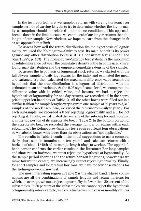
Option-Implied Risk-Neutral Distributions and Risk Aversion
©2004, The Research Foundation of AIMR™ 41
In the test reported here, we sampled returns with varying horizons oversample periods of varying lengths to try to determine whether the lognormal-ity assumption should be rejected under these conditions. This approachbreaks down in the limit because we cannot calculate longer returns than thelength of our sample. Nevertheless, we hope to learn from the changes in fitas we approach that limit.
To assess how well the return distribution fits the hypothesis of lognor-mality, we used the Kolmogorov–Smirnov test. Its main benefit is its poweragainst any other distribution because it is a consistent test (Kendall andStuart 1979, p. 483). The Kolmogorov–Smirnov test statistic is the maximumabsolute difference between the cumulative density of the hypothesized (here,lognormal) distribution and the empirical cumulative density of the sample.
To assess the hypothesis of lognormal stock returns, we started with thefull 69-year sample of daily log returns for the index and estimated the meanand variance. We then calculated the maximum difference value against thehypothesis that the true distribution is a lognormal distribution with theestimated mean and variance. At the 0.05 significance level, we compared thedifference value with its critical value, and because we had to reject thehypothesis of lognormality for one-day returns, we recorded a 0 in the appro-priate upper left-hand box of Table 2. All the other boxes were filled out in asimilar fashion for sample lengths varying from one sample of 69 years to 3,312samples of one week each. Also, we varied the returns from daily to yearly. Foreach subsample, we recorded a 0 for rejecting lognormality and a 1 for notrejecting it. Finally, we calculated the average of the subsamples and recordedit in the top portion of its appropriate box in Table 2. In the bottom portion ofthe appropriate box, we recorded the average number of returns within eachsubsample. The Kolmogorov–Smirnov test requires at least four observations,so we labeled boxes with fewer than six observations as “not applicable.”
The results in Table 2 confirm the initial suggestions to use a compara-tively short sample (months to a few years) and calculate returns with ahorizon of about 1/40th of the sample length (days to weeks). The upper left-hand corner confirms the earlier results in the literature: For long samplesand short return horizons, we must reject the hypothesis of lognormality. Asthe sample period shortens and the return horizon lengthens, however (as wemove toward the center), we increasingly cannot reject lognormality. Finally,for short samples and long return horizons, we have too few observations forthe Kolmogorov–Smirnov test.
The most interesting region in Table 2 is the shaded band. These combi-nations are all the combinations of sample lengths and return horizons forwhich, on average, we must reject lognormality in fewer than 20 percent of thesubsamples. In 80 percent of the subsamples, we cannot reject the hypothesisof lognormality—for example, weekly returns over one year or monthly returns
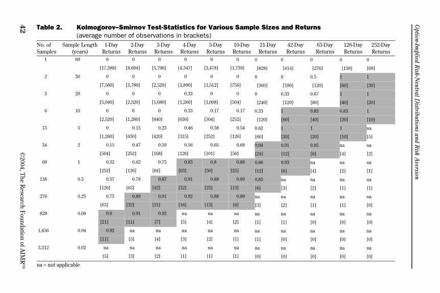
Option-Im
plied Risk-N
eutral Distributions and R
isk Aversion
42
©2004, The R
esearch Foundation of AIM
R™
Table 2. Kolmogorov–Smirnov Test-Statistics for Various Sample Sizes and Returns(average number of observations in brackets)
No. of Samples
Sample Length(years)
1-Day Returns
2-Day Returns
3-Day Returns
4-Day Returns
5-Day Returns
10-Day Returns
21-Day Returns
42-Day Returns
63-Day Returns
126-Day Returns
252-Day Returns
1 69 0 0 0 0 0 0 0 0 0 0 0
[17,388] [8,694] [5,796] [4,347] [3,478] [1,739] [828] [414] [276] [138] [69]
2 30 0 0 0 0 0 0 0 0 0.5 1 1
[7,560] [3,780] [2,520] [1,890] [1,512] [756] [360] [180] [120] [60] [30]
3 20 0 0 0 0.33 0 0 0 0.33 0.67 1 1
[5,040] [2,520] [1,680] [1,260] [1,008] [504] [240] [120] [80] [40] [20]
6 10 0 0 0 0.33 0.17 0.17 0.33 1 0.83 0.83 1
[2,520] [1,260] [840] [630] [504] [252] [120] [60] [40] [20] [10]
13 5 0 0.15 0.23 0.46 0.38 0.54 0.62 1 1 1 na
[1,260] [630] [420] [315] [252] [126] [60] [30] [20] [10] [5]
34 2 0.15 0.47 0.59 0.56 0.65 0.68 0.94 0.91 0.85 na na
[504] [252] [168] [126] [101] [50] [24] [12] [8] [4] [2]
69 1 0.32 0.62 0.75 0.83 0.8 0.88 0.88 0.93 na na na
[252] [126] [84] [63] [50] [25] [12] [6] [4] [2] [1]
138 0.5 0.57 0.78 0.87 0.91 0.88 0.89 0.85 na na na na
[126] [63] [42] [32] [25] [13] [6] [3] [2] [1] [1]
276 0.25 0.75 0.89 0.91 0.92 0.88 0.89 na na na na na
[63] [32] [21] [16] [13] [6] [3] [2] [1] [1] [0]
828 0.08 0.9 0.91 0.92 na na na na na na na na
[21] [11] [7] [5] [4] [2] [1] [1] [0] [0] [0]
1,656 0.04 0.92 na na na na na na na na na na
[11] [5] [4] [3] [2] [1] [1] [0] [0] [0] [0]
3,312 0.02 na na na na na na na na na na na
[5] [3] [2] [1] [1] [1] [0] [0] [0] [0] [0]
na = not applicable

Option-Implied Risk-Neutral Distributions and Risk Aversion
©2004, The Research Foundation of AIMR™ 43
over two years. Even for favorites of financial practitioners—such as threemonths of daily returns (for estimating the historical volatility for optionpricing) and five years of monthly returns (for asset pricing)—we must rejectlognormality for only 25 percent and 38 percent of the subsamples, respectively.
For a number of applications, the assumption of lognormally distributedreturns may hold reasonably well. Often, it holds for a short sample withreturns measured over a longer horizon, such as a month, for two reasons.One reason is that the sample mean is noisy so it is likely to be useless nomatter how long a sample is chosen. In this case, the sample mean might bepicked some other way—by, say, assuming it is the risk-free rate plus areasonable risk premium. Second, the sample variance is somewhat insensi-tive to the return horizon and can reasonably be scaled up or down by thesquare root of time. Thus, we might be able to use a short sample with shorthorizon returns for the variance estimate. Even alternative variance esti-mates—from option-implied volatility, for example—could be used.
Implied Binomial TreesOnce we understand how to obtain risk-neutral probability distributions at aparticular date, we are tempted to ask what we can infer about the stochasticprocess of the underlying asset that leads to this terminal distribution. In adeep and liquid options market, such as the S&P 500 options market, we cansimultaneously find as many as 100 different quotes for options of differenttimes to expiration and different strike prices. There is no unique stochasticprocess consistent with these option prices, however, and even if we were toknow the risk-neutral probability distributions for every instant of time, therewould still not be a unique stochastic process. The reason is that there couldbe stochastic jumps, stochastic interest rates, or stochastic volatility—any ofwhich will give rise to multiple processes consistent with observed prices. Thisproblem is related to the problem of market incompleteness: If we encountertoo many possible states and we have too few securities and too few tradingopportunities, several risk-neutral stochastic processes are feasible that willprice the observed securities correctly.
Only if we are willing to limit ourselves to single-factor diffusion processeswill we obtain a unique stochastic process. And implied binomial trees aresimply discretizations of such generalized one-dimensional diffusion pro-cesses, in which the volatility parameter is a general function of time and theasset price. This feature sets implied binomial trees apart from the Black–Scholes formula, in which volatility is constant.16 The drift of the implied
16 The associated Cox–Ross–Rubinstein tree is a discretization of the Black–Scholes economyand shares this feature of exhibiting constant volatility.

Option-Implied Risk-Neutral Distributions and Risk Aversion
44 ©2004, The Research Foundation of AIMR™
binomial tree is equal to the risk-free rate when we work with risk-neutralprobabilities. The pioneers of this literature are Rubinstein (1994), Dermanand Kani (1994), and Dupire (1994). After describing their work, we will turnto recent extensions.
Rubinstein’s Implied Binomial Trees. The simple two-step Cox–Ross–Rubinstein binomial tree serves well as an introduction to impliedbinomial trees. A binomial tree is a discretization of the Black–Scholes model.We assume a volatility of 0.2, a current stock price, S, of 1, and a risk-free rateof return, r, of 1.1. We further assume that no dividends are paid and that eachperiod lasts one year. Figure 7 exhibits the nodal stock prices and probabil-ities for the standard binomial tree.
We now complicate the situation by introducing a volatility smile. Forevery 10 percentage points of moneyness subtracted from the at-the-moneyoption, we increase volatility by a factor of 1.1 and we do the inverse forincreases in moneyness. A two-year call option with a strike price of 1.1 nowhas an implied volatility of 0.2/1.1 = 0.1818 and a price of 0.1497.
Figure 7. Standard Binomial Tree
1.4918
1.2214
1
0.8187
1.0000
0.6703
0.4879
0.6985
1
0.3015
0.4212
0.0909
A. Stock Prices
B. Nodal Probabilities
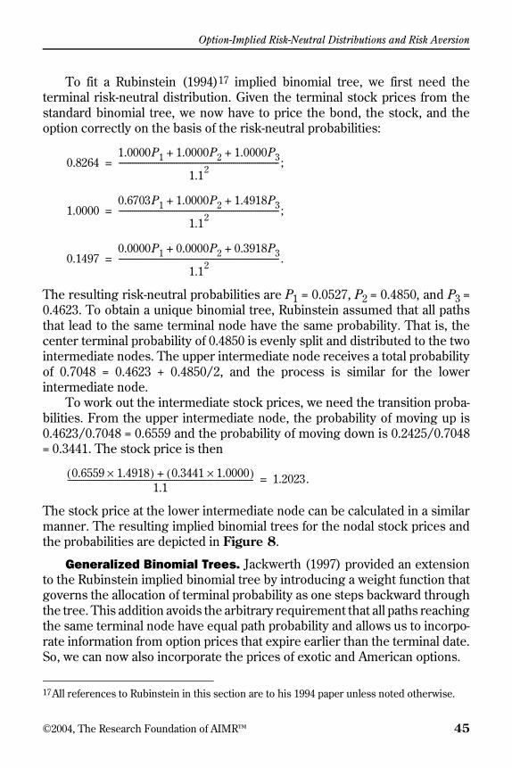
Option-Implied Risk-Neutral Distributions and Risk Aversion
©2004, The Research Foundation of AIMR™ 45
To fit a Rubinstein (1994)17 implied binomial tree, we first need theterminal risk-neutral distribution. Given the terminal stock prices from thestandard binomial tree, we now have to price the bond, the stock, and theoption correctly on the basis of the risk-neutral probabilities:
The resulting risk-neutral probabilities are P1 = 0.0527, P2 = 0.4850, and P3 =0.4623. To obtain a unique binomial tree, Rubinstein assumed that all pathsthat lead to the same terminal node have the same probability. That is, thecenter terminal probability of 0.4850 is evenly split and distributed to the twointermediate nodes. The upper intermediate node receives a total probabilityof 0.7048 = 0.4623 + 0.4850/2, and the process is similar for the lowerintermediate node.
To work out the intermediate stock prices, we need the transition proba-bilities. From the upper intermediate node, the probability of moving up is0.4623/0.7048 = 0.6559 and the probability of moving down is 0.2425/0.7048= 0.3441. The stock price is then
The stock price at the lower intermediate node can be calculated in a similarmanner. The resulting implied binomial trees for the nodal stock prices andthe probabilities are depicted in Figure 8.
Generalized Binomial Trees. Jackwerth (1997) provided an extensionto the Rubinstein implied binomial tree by introducing a weight function thatgoverns the allocation of terminal probability as one steps backward throughthe tree. This addition avoids the arbitrary requirement that all paths reachingthe same terminal node have equal path probability and allows us to incorpo-rate information from option prices that expire earlier than the terminal date.So, we can now also incorporate the prices of exotic and American options.
17All references to Rubinstein in this section are to his 1994 paper unless noted otherwise.
0.82641.0000P1 1.0000P2 1.0000P3+ +
1.12--------------------------------------------------------------------------------- ;=
1.00000.6703P1 1.0000P2 1.4918P3+ +
1.12--------------------------------------------------------------------------------- ;=
0.14970.0000P1 0.0000P2 0.3918P3+ +
1.12--------------------------------------------------------------------------------- .=
0.6559 1.4918×( ) 0.3441 1.0000×( )+1.1
---------------------------------------------------------------------------------------------- 1.2023.=

Option-Implied Risk-Neutral Distributions and Risk Aversion
46 ©2004, The Research Foundation of AIMR™
A one-year call option with strike price 1.1 would be priced on Rubinstein’simplied binomial tree at
but let us assume that the observed market price is 0.0724. In this case, aproperly fitted generalized binomial tree can match the observed option priceby splitting the center terminal probability of 0.4850, not evenly, but sendingonly 41.90 percent up to the intermediate upper node and sending 58.10percent down. The upper intermediate node then receives a total probabilityof 0.6655 = 0.4623 + 0.2032 and the lower intermediate node is calculatedsimilarly. We also recalculate the stock price tree in the manner described,and the resulting generalized binomial trees for the nodal stock prices andprobabilities are as depicted in Figure 9.
Derman–Kani Trees. Derman and Kani (1994) introduced yet a differentimplied tree.18 Their tree is constructed by building it up node by node byusing the information in an option that expires on that particular time step and
Figure 8. Implied Binomial Tree
18All references to Derman and Kani in this section are to their 1994 paper unless notedotherwise.
0.4623
0.7048
1
0.2952
0.4850
0.0527
1.4918
1.2023
1
0.8556
1.0000
0.6703
A. Stock Prices
B. Nodal Probabilities
0.7048 0.1023×( ) 0.2952 0.0000×( )+1.1
---------------------------------------------------------------------------------------------- 0.0656,=
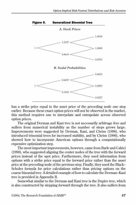
Option-Implied Risk-Neutral Distributions and Risk Aversion
©2004, The Research Foundation of AIMR™ 47
has a strike price equal to the asset price of the preceding node one stepearlier. Because these exact option prices will not be observed in the market,this method requires one to interpolate and extrapolate across observedoption prices.
The original Derman and Kani tree is not necessarily arbitrage free andsuffers from numerical instability as the number of steps grows large.Improvements were suggested by Derman, Kani, and Chriss (1996), whointroduced trinomial trees for increased stability, and by Chriss (1996), whoshowed how to incorporate American options through a computationallyexpensive optimization step.
The most important improvements, however, came from Barle and Cakici(1998), who suggested aligning the center nodes of the tree with the forwardprices instead of the spot price. Furthermore, they used information fromoptions with a strike price equal to the forward price rather than the assetprice at the preceding node of the previous step. Finally, they used the Black–Scholes formula for price calculations rather than pricing options on thecoarse binomial tree. A detailed example of how to calculate the Derman–Kanitree is provided in Appendix B.
Somewhat similar to the Derman and Kani tree is the Dupire tree, whichis also constructed by stepping forward through the tree. It also suffers from
Figure 9. Generalized Binomial Tree
0.4623
0.6655
1
0.3345
0.4850
0.0527
1.4918
1.2197
1
0.8619
1.0000
0.6703
A. Stock Prices
B. Nodal Probabilities
Option-Implied Risk-Neutral Distributions and Risk Aversion
48 ©2004, The Research Foundation of AIMR™
numerical difficulties, however, and for this reason, backward-stepping treesare preferable. Cont, Da Fonseca, and Durrleman (2002) observed that theforward smile in a Derman and Kani tree cannot be time invariant. Rather,future smiles necessarily flatten out as time evolves, which is contrary to theempirical smile’s behavior. A parametric tree model of interest in this contextis the one developed by Guidolin and Timmermann, who modeled the stockprice evolution on a tree when Bayesian learning occurs about dividend news.Their model generates symmetrical volatility smiles but not skews.
The best choice of this group seems to be the generalized binomial tree(see Jackwerth 1997) because it can incorporate information on observedexotic and American option prices. It is guaranteed to be arbitrage free, but acomplete fit involves nonlinear optimization. One can avoid nonlinear optimi-zation in the forward-stepping trees, for which I recommend using the Barle–Cakici version of the Derman–Kani tree.
Two-Factor Implied Trees. Implied binomial trees have also beenextended to incorporate additional stochastic factors—stochastic volatilityand stochastic implied volatility.
Derman and Kani (1998) fitted an implied trinomial tree with initially fixedtransition probabilities. They then specified an exogenous stochastic processof how these transition probabilities can change. The methodology is relatedto the interest rate model of Heath, Jarrow, and Morton (1992), and it similarlyintroduces path dependence. That is, the implied tree is no longer recombin-ing and the number of nodes explodes. Option prices can then be calculatedonly via MONTE CARLO SIMULATION.
Britten-Jones and Neuberger (2000) obtained the set of continuous sto-chastic processes that is compatible with observed option prices and thatgenerates the same volatility forecast. They also used implied trinomial trees,for which they specified the volatility process as a discrete Markov chain. Theyintroduced transition probabilities with which the process moves from onevolatility state to the next. Although their model is more restricted than thatof Derman and Kani (1998), it is also much faster to compute because itrequires no Monte Carlo simulation. Neither of these models has so far beentested empirically.
Recently, a line of research has approached modeling stochastic impliedvolatilities as opposed to stochastic local volatilities. A motivation for thisresearch is that practitioners like to work with the implied volatility surfaceas an ad hoc pricing model. Berkowitz (2001) established that this approach,when the surface is frequently updated, can provide accurate forecasts offuture option prices. Dumas, Fleming, and Whaley (1998) gave credence tothis argument because their deterministic volatility model performed better
Option-Implied Risk-Neutral Distributions and Risk Aversion
©2004, The Research Foundation of AIMR™ 49
when implied, rather than when local, volatilities were used. Model risk,however, affects different options differently. Hull and Suo (2002) fitted acontinually recalibrated deterministic volatility model to simulated Europeanoption prices written on a stochastic volatility process. They found thatdeterministic volatility models are better at pricing and hedging compoundoptions than certain barrier options.
Ledoit and Santa-Clara (1998) and Amerio, Fusai, and Vulcano (2001)derived conditions under which the joint process of stock price and volatilitysurface is arbitrage free. Cont et al. modeled the implied volatility surface asa three-factor MEAN-REVERTING DIFFUSION, in which the factors correspond tochanges in level, tilt, and curvature. (The choice of these factors was guidedby the principal component analysis of the implied volatility surface in Contand Da Fonseca 2002.) This restricted process is calibrated to observed optionprices and can be used to price illiquid or exotic options via Monte Carlosimulation.
In a method similar to modeling the dynamics of the implied volatilities,Panigirtzoglou and Skiadopoulos (2002) directly modeled the evolution of therisk-neutral and cumulative risk-neutral distribution. They used principalcomponent analysis and rotated the principal components to arrive at a two-component (two-factor) model in which the first factor is a level shift and thesecond factor is a change in curvature. Again, they simulated future distribu-tions via a Monte Carlo algorithm and suggested a VAR application. Skia-dopoulos and Hodges (2001) also modeled the evolution of risk-neutralmixtures of distributions when the mean or variance changes stochastically.
Other Nonparametric Models. One way to discretize the generalizedvolatility surface of a diffusion process is to build an implied binomial tree.This choice is particularly convenient, but alternatively, we could specify arectangular grid in time and asset prices in which we would record the localvolatilities. This alternative was proposed by Dumas, Fleming, and Whaleyand is called the “deterministic volatility model.” With this model, one can usefinite-difference methods to price options. Andersen and Brotherson-Ratcliffe(1997) had already suggested this methodology and described various(implicit and semi-implicit) finite-difference algorithms. He argued that deter-ministic volatility models have computational advantages over implied bino-mial trees for valuing options with discontinuous payoffs, such as barrieroptions.
A number of authors have proposed deterministic volatility models withthe additional requirement that the volatility surface be smooth. Bodurtha andJermakyan (1996a, 1996b) and Lagnado and Osher (1997a, 1997b) are exam-ples. But the authors all acknowledged that their algorithms are computation-
Option-Implied Risk-Neutral Distributions and Risk Aversion
50 ©2004, The Research Foundation of AIMR™
ally expensive. Coleman, Li, and Verma (1999) found the required smoothvolatility surface by using bicubic splines, which eases the computationalcost.19 Avellaneda, Friedman, Holmes, and Samperi (1997) achieved thesmoothness by maximizing the cross-entropy of the fitted volatility surfaceand a prior surface. Their method suffers from numerical difficulties, however,because it exhibits severe spikes. Bouchouev and Isakov (1997) built up thevolatility surface from rather complicated functions involving integral evalua-tions. They assumed that the volatility surface does not change over time,which severely restricts the flexibility of their algorithm. Brigo and Mercurio(2002) extended the mixture of distributions method to a mixture of lognormaldiffusions that are all driven by the same Brownian motion. The result is aparametric volatility surface with a closed-form option-pricing formula.
Carr and Madan (2001) added more structure to the volatility surface ofa deterministic volatility model by assuming that the asset price itself is pathindependent. This assumption implies that the asset price depends only ontime and the level of the underlying diffusion process. With this additionalassumption, the whole volatility surface can be obtained by observing one setof option prices with a common time to expiration. This information willnormally yield only one risk-neutral probability distribution, not a completedeterministic volatility model. Carr, Tari, and Zariphopoulou (1999) describedvolatility surfaces that yield closed-form option-pricing formulas and gavesome examples.
Laurent and Leisen (1998) added structure in a different way by restrictingasset prices to lie on a prespecified grid. They modeled the transition proba-bilities from one node of the grid to another as a Markov chain. Their modelimplies an incomplete market because more states can be reached than thereare available assets. Thus, they suggested either picking the risk-neutralprobability distribution that yields the highest prices for all of the nontradedassets or using cross-entropy maximization to find a risk-neutral distributionthat is closest to a prior distribution and still fits the observed option prices.Of these two choices, using cross-entropy maximization seems to make moreeconomic sense; the first choice will give only an upper bound on option prices.Also investigating incomplete markets, Samperi (1996) gave bounds for optionprices if the volatility surface of a deterministic volatility model is boundedbetween an upper and a lower bound. Assuming that investors follow risk-minimizing trading strategies, Samperi obtained a unique implied tree.
All the models described so far kept some structure for the underlyingstochastic process—namely, a generalized diffusion. A final class of nonpara-
19“Bicubic” means order 3 in the local polynomials in both dimensions (time and asset value).
Option-Implied Risk-Neutral Distributions and Risk Aversion
©2004, The Research Foundation of AIMR™ 51
metric models, however, does away with this structure completely. Kernelmethods, such as that of Aït-Sahalia and Lo (1998), view the option-pricingmodel as a mere exercise in interpolation and extrapolation of observedmarket option prices, which can be done in terms of option prices or impliedvolatilities. They proposed fitting a five-dimensional surface of option-impliedvolatilities across stock prices, strike prices, times to expiration, interest rates,and dividend yields.
Closely related in spirit are NEURAL NETWORKS, which are nonlinear regres-sion methods with functional forms that are flexible because of the layered useof such simple functions as f(x) = 1/(1 + e–x). These simple functions are appliedto the data and then combined in weighted sums. The nodal sums of a particularlayer are then used as input to the simple functions again, and weighted sumsare calculated once more, yielding still fewer nodes at the second layer. Afterseveral layers, the method culminates in one single nodal value. Hutchinson,Lo, and Poggio (1994) used such a neural network on simulated Black–Scholesoption prices to recover the Black–Scholes pricing formula, and they also fittedobserved option prices on S&P 500 futures. Herrmann and Narr (1997) useda neural network on German index option prices.
Empirical Tests. Because of the dual difficulty of dealing with compli-cated option-pricing models and the paucity of large option price datasets, onlytwo extensive studies with large samples have tested the performance ofimplied binomial trees. Dumas et al. approximated the volatility surface of theirdeterministic volatility model with polynomials in time and asset price. I willdescribe here a version of their model in which one fits the implied volatilitysurface, because this ad hoc extension works slightly better than the originalversion. For every Wednesday from June 1988 through December 1993, theyfitted the volatility surface to observed prices of options on the S&P 500. Oneweek later, they priced all options on the basis of the week-old volatility surface,where they conditioned on the change in time and asset price. These modelprices were compared with market prices, and the average root mean squaredprediction error was found to range from 47 cents to 59 cents for options withtime to expiration of more than 70 days. The authors compared this predictionerror with an average bid–ask spread of 47 cents and judged the deterministicvolatility model to be generally poor.
Lim and Zhi (2002) presented findings of a more limited study of gener-alized binomial trees and Derman–Kani trees fitted to the British FTSE 100options. The Derman–Kani trees come out ahead, but both models stillapparently contain biases.
Option-Implied Risk-Neutral Distributions and Risk Aversion
52 ©2004, The Research Foundation of AIMR™
Fully parametric models have not fared much better. Bakshi et al. fittedparametric stochastic jump/stochastic volatility models to S&P 500 optionsfrom June 1988 through May 1991. They did not report one-week predictionerrors but reported one-day prediction errors of about 40 cents for optionswith time to expiration of 60–180 days.
The only paper to simultaneously consider parametric methods (includ-ing a stochastic volatility model), implied binomial trees, and naive tradingrules is Jackwerth and Rubinstein (1998). The naive trading rules simplyassumed that the implied volatility smile in terms of strike prices (absolutemodel) or across moneyness (relative model) stays constant through time.The authors used options on the S&P 500 from April 1986 through December1995 and fitted all models to daily observations of option prices. They reportedthe prediction errors of two-week forecasts for options with time to expirationof 135–215 days. The errors were lowest (57 cents) for the naive trading rulesand similar for the implied binomial trees (75 cents) and the parametricmodels (78 cents). These prediction errors are noisy observations, whichmakes it difficult to distinguish the predictive power of the various models.Although more research into this question is certainly warranted, to dismissimplied binomial tree models at this time would be premature.
Applications and Use. Consider how an investment professional canuse implied binomial trees. The applications are much more limited than inthe case of the risk-neutral distributions for two reasons. First, the technologyinvolved to set up implied binomial trees is much more complicated than thetechnology for obtaining a single risk-neutral distribution. And the singledistribution is less sensitive to noise in the data than the same density viewedas part of a larger implied binomial tree. Second, information provided by animplied binomial tree in addition to the risk-neutral distribution is plainlyoverkill for most applications.
The only real reason to use implied binomial trees is to value exoticoptions, which depend on the complete stochastic process through timerather than simply the terminal risk-neutral distribution. For such options, theeffort of calibrating an implied binomial tree to a whole range of vanilla optionswith different times to expiration makes sense despite the difficulties. For anyother application, such as risk management, portfolio management, or fore-casting, practitioners can reasonably concentrate on a particular horizon andwork with the risk-neutral distribution at that date.
Implied Risk AversionIn pricing securities, we discount the expected payoff of the security when weuse risk-neutral probabilities, which will normally differ from the actual prob-
Option-Implied Risk-Neutral Distributions and Risk Aversion
©2004, The Research Foundation of AIMR™ 53
abilities. The reason is that investors are typically risk averse. That is, promis-ing a dollar payoff to a U.S investor in a state of the world when the investor isalready wealthy is worth less to the investor than in a state where the investoris poor. The investor will, therefore, lower his or her actual probabilities toarrive at risk-neutral probabilities for pricing purposes. Similarly, the investorwill raise the actual probability to arrive at a higher risk-neutral probability fordollars obtained in states of the world when he or she is poor.
In an economy in which such an investor is the representative agent andalone determines all prices, we can explicitly relate the ratio of risk-neutralprobabilities, P, to actual probabilities, Q, to the scaled marginal utility, U′/ξ,which is also called the “pricing kernel,” m, of the representative agent:
(12)
where ξ is the shadow price of the budget constraint. The scaling by ξ doesnot affect any of our results, and we will use the terms “pricing kernel” and“marginal utility” interchangeably.
Empirical Estimates of Risk Aversion and Pricing Kernels. Once weaccept that the risk-neutral distribution is not the same as the actual distribu-tion, we can try to estimate the two distributions and divide them into eachother to obtain empirical functions of scaled marginal utility. Bartunek andChowdhury (1997) were the first to do so, but they restricted the utilityfunction to be of the power utility type. They fitted a lognormal distribution toS&P 100 Index returns and estimated risk aversion coefficients between 0.2and 0.6 from fitting S&P 100 option prices. These values appear to be low whencompared with surveys that suggest coefficients of 2–5. Bliss and Panigirtzo-glou (2002) used the same parameterization and added exponential utilityfunctions. Using data for the British FTSE 100 Index returns and options andS&P 500 returns and options, they found rather moderate risk-aversion esti-mates—between 2 and 7—whereas the equity premium literature suggestsmuch higher values (e.g., 55 from Mehra and Prescott 1985). A problem withthese approaches is that they parameterize the utility function rather thanestimating it as a nonparametric function from the data.
A number of papers have estimated the risk-neutral distribution, however,by using one of the methods described in the section “The Inverse Problem.”The authors obtained the actual distribution from fitting a time-series modelto the index returns and divided the probability distributions to arrive at
m U′ξ
------=
PrTQ---------- ,=
Option-Implied Risk-Neutral Distributions and Risk Aversion
54 ©2004, The Research Foundation of AIMR™
nonparametric empirical functions of scaled marginal utility. Using data fromthe S&P 500 options market, Aït-Sahalia and Lo (2000) used kernel methodsfor both distributions. Rosenberg and Engle fitted a curve to the impliedvolatility smile to obtain the risk-neutral distribution and fitted a GARCHmodel to the index returns. Coutant (2000) used Hermite polynomials for therisk-neutral distribution and fitted an ARCH-type model to the French CAC 40Index. Also using the CAC 40, Perignon and Villa used kernel methods forfitting both the implied volatility smile and the historical return distribution.Hayes and Shin used a cubic spline to fit the implied volatilities across deltasin combination with a GARCH model for the S&P 500 returns. They focusedon the –20 percent return event, however, and worked out the time series ofmarginal utility estimates for these large crashes, during which marginalutility tends to be high.
In a related method, Henrotte (2002) suggested an algorithm to obtainthe pricing kernel with the smallest increase in the optimal dynamic Sharperatio while still pricing observed securities correctly. Chernov (2000) specifiedthe stochastic processes that drive the economy and was then able to estimatethe implied pricing kernel from time series on stocks, interest rates, andfutures.
The Pricing Kernel Puzzle. Jackwerth (2000) used the implied risk-aversion functions, which are closely related to marginal utility functions (theyare the negatives of the derivative of log marginal utility) and documented aso-called pricing kernel puzzle. He found that the implied marginal utilityfunction is monotonically decreasing across wealth in a precrash period, aseconomic theory would suggest. That is, people grow less appreciative ofadditional wealth as they become wealthier. This picture changes during thepostcrash period, however, when the implied marginal utility function islocally increasing in wealth for wealth levels close to the starting wealth level.The studies of Rosenberg and Engle (2002) and of Perignon and Villa con-firmed these findings. Aït-Sahalia and Lo (2000) and Bliss and Panigirtzoglou(2002), however, did not find such an effect. Aït-Sahalia and Lo used a wholeyear of option price data and averaged the information, but these authors mayhave smoothed their kernel estimates too much. Bliss and Panigirtzoglouused a parametric form of the utility function, which precluded finding apotential pricing kernel puzzle a priori.
To provide an understanding of the pricing kernel puzzle, Figure 10 depictsempirical estimates of the risk-neutral and the actual distributions for fourinternational indexes. The actual distributions appear to be somewhat(log)normally distributed, whereas the risk-neutral distributions are (exceptfor Japan) left skewed and leptokurtic; that is, they have fat left tails and are
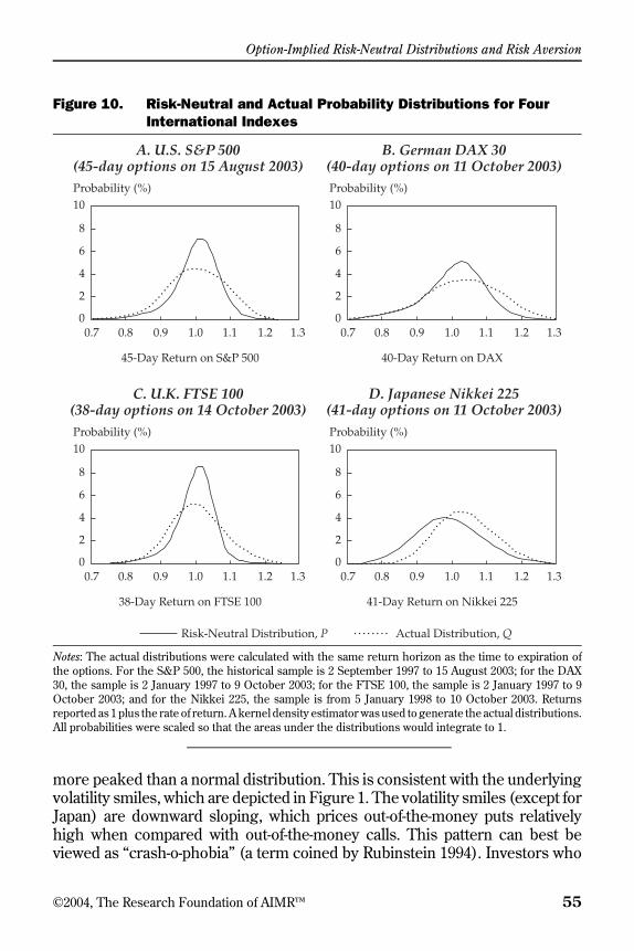
Option-Implied Risk-Neutral Distributions and Risk Aversion
©2004, The Research Foundation of AIMR™ 55
more peaked than a normal distribution. This is consistent with the underlyingvolatility smiles, which are depicted in Figure 1. The volatility smiles (except forJapan) are downward sloping, which prices out-of-the-money puts relativelyhigh when compared with out-of-the-money calls. This pattern can best beviewed as “crash-o-phobia” (a term coined by Rubinstein 1994). Investors who
Figure 10. Risk-Neutral and Actual Probability Distributions for Four International Indexes
Notes: The actual distributions were calculated with the same return horizon as the time to expiration ofthe options. For the S&P 500, the historical sample is 2 September 1997 to 15 August 2003; for the DAX30, the sample is 2 January 1997 to 9 October 2003; for the FTSE 100, the sample is 2 January 1997 to 9October 2003; and for the Nikkei 225, the sample is from 5 January 1998 to 10 October 2003. Returnsreported as 1 plus the rate of return. A kernel density estimator was used to generate the actual distributions.All probabilities were scaled so that the areas under the distributions would integrate to 1.
Probability (%)10
8
2
4
6
00.7 1.30.8 0.9 1.0 1.21.1
38-Day Return on FTSE 100 41-Day Return on Nikkei 225
45-Day Return on S&P 500 40-Day Return on DAX
A. U.S. S&P 500(45-day options on 15 August 2003)
B. German DAX 30(40-day options on 11 October 2003)
C. U.K. FTSE 100(38-day options on 14 October 2003)
Probability (%)
D. Japanese Nikkei 225(41-day options on 11 October 2003)
10
8
2
4
6
00.7 1.30.8 0.9 1.0 1.21.1
Probability (%)10
8
2
4
6
00.7 1.30.8 0.9 1.0 1.21.1
Probability (%)10
8
2
4
6
00.7 1.30.8 0.9 1.0 1.21.1
Risk-Neutral Distribution, P Actual Distribution, Q

Option-Implied Risk-Neutral Distributions and Risk Aversion
56 ©2004, The Research Foundation of AIMR™
are concerned about market crashes insure themselves by buying out-of-the-money puts, which put a floor on the maximum losses the investors can sustain.The prices of these puts are then pushed up because only a few investmentbanks and hedge funds are willing to supply such insurance in large quantity.
We are now ready to divide the two probability distributions into eachother to obtain the empirical pricing kernels for the four international indexes,which are shown in Figure 11. Notice that the empirical pricing kernels are,as expected, broadly downward sloping as wealth increases. This pattern isan indication of risk-averse investors in the economy. The pricing kernelpuzzle is that, theoretically, the pricing kernel should be monotonicallydecreasing but, at times, it increases for wealth levels close to the startingwealth level of 1. An implication of locally increasing pricing kernels is thatthe utility functions of the investors are locally convex. In that case, theinvestors would actually pay to obtain a fair gamble instead of simply pocketingthe expected value of the gamble for sure. For most investors, such behavioris inconsistent with reality and contradicts our assumption that the represen-tative investors in the different countries are risk averse. Still, the relationshipthat marginal utility is proportional to the ratio of risk-neutral probability andactual probability is based on this assumption. This is the puzzle, and a numberof research papers have examined it.
Before we dive into possible solutions to the pricing kernel puzzle, weneed to establish that it is not merely an artifact of our estimation method.Based on the dataset of daily option, bond, and index returns of Buraschi andJackwerth, the pricing kernel puzzle can be confirmed at the daily horizon forthe S&P 500. Moreover, our assumptions for the estimation are not onerous.To estimate the risk-neutral distribution, we need only assume that theobserved option prices are arbitrage free. For the estimation of the actualdistribution, we need to assume rational expectations. These two assumptionsare commonly made in empirical work and we will do so here.
Jackwerth (2000) investigated the underlying data (on the S&P 500) andmethodology in detail and did not find any problems. In particular, usingvarious methodologies to obtain the distributions did not change the results.The results were also statistically significant: They occurred for every monthin the more than eight years of data starting in June 1988 and ending inNovember 1995. The pricing kernel puzzle occurs in the center of the distri-bution and is thus not affected by mispricing of away-from-the-money options.Also, liquidity is highest around the center of the distribution, so details ofmarket microstructure (such as bid–ask spreads, transaction costs, or marginrequirements) are not likely to be causing the pricing kernel puzzle becausenone of those frictions changed dramatically around the crash of 1987; thepricing kernel puzzle came into existence instantaneously.

Option-Implied Risk-Neutral Distributions and Risk Aversion
©2004, The Research Foundation of AIMR™ 57
Solutions to the Pricing Kernel Puzzle. The existing literature islargely one-sided, in that either the risk-neutral distribution or the actualdistribution is being modeled; almost no work links the two aspects in termsof the pricing kernel as the scaled ratio of the two. For example (morereferences can be found in the section “Empirical Findings,” where I discussedthese works from a different perspective), the leverage effect suggests that asmarket values fall, the market debt-to-equity ratio (and thus index volatility)increase. As a result, we see downward-sloping implied volatility smiles, suchas in Figure 1 (except for Japan). Black and others discussed the leverage
Figure 11. Empirical Pricing Kernels for Four International Indexes
Note: The pricing kernels were calculated as the ratio of the option-implied risk-neutral distribution andthe actual distribution based on historical smoothed returns.
Pricing Kernel, m5
2
1
4
3
00.7 1.30.8 0.9 1.0 1.21.1
38-Day Return on FTSE 100 41-Day Return on Nikkei 225
45-Day Return on S&P 500 40-Day Return on DAX
A. U.S. S&P 500(45-day options on 15 August 2003)
B. German DAX 30(40-day options on 11 October 2003)
C. U.K. FTSE 100(38-day options on 14 October 2003)
Pricing Kernel, m
D. Japanese Nikkei 225(41-day options on 11 October 2003)
5
2
1
4
3
00.7 1.30.8 0.9 1.0 1.21.1
Pricing Kernel, m5
2
1
4
3
00.7 1.30.8 0.9 1.0 1.21.1
Pricing Kernel, m5
2
1
4
3
00.7 1.30.8 0.9 1.0 1.21.1

Option-Implied Risk-Neutral Distributions and Risk Aversion
58 ©2004, The Research Foundation of AIMR™
effect in terms of the actual distribution; Toft and Prucyk and Dennis andMayhew discussed it in terms of the risk-neutral distribution. None of thesepapers, however, connected the two aspects in terms of the pricing kernel.
The correlation effect suggests that in down markets, correlationsbetween companies increase, so the impact of additional bad news is asym-metrical. From a different perspective, the information effect assumes thatinvestors learn through trading, so prices can, at times, adjust sharply evenwithout any news. Both of these effects are capable of producing a downward-sloping volatility smile, but no author has modeled the two distributionsjointly.
A different line of research involves actually modeling the pricing kerneldirectly. This approach includes Franke, Stapleton, and Subrahmanyam(1998, 1999) with their models of background risk. Benninga and Maysharconsidered heterogeneous investors, and Campbell and Cochrane (2000)modeled habit persistence—in which investors get used to their current levelsof consumption and derive utility only from an increase in consumptionbeyond those levels. Grossman and Zhou modeled the demand and supply ofportfolio insurance. But all these models have in common that their pricingkernels are monotonically decreasing in wealth, and therefore, the models donot address the pricing kernel puzzle.
Finally, a number of continuous-time models have extended the geomet-ric Brownian motion of the Black–Scholes model. Heston’s work and theGARCH model of Duan (1995), for example, introduced stochastic volatility,and Bakshi et al, Bates (2000), and Pan introduced stochastic jumps in theindex and in the volatility of the index. These models move back and forthbetween the risk-neutral and the actual stochastic process (and their associ-ated probability distributions) by assuming that the price of risk is propor-tional to the volatility or to the intensity of the jump. Alas, this particularassumption about the price of risk combined with reasonable parameterestimates leads, again, to monotonically decreasing pricing kernels. Thisoutcome is depicted in Figure 12 for the simulations of Pan’s model, forwhich her estimated parameters were used.
Only a few papers have expressly dealt with the pricing kernel puzzle:Branger and Schlag (2002), Ziegler, and Brown and Jackwerth (2003).
Branger and Schlag considered an economy in which the index is com-posed of 30 stocks with both idiosyncratic and systematic diffusion compo-nents and also idiosyncratic and systematic jump components in theirstochastic processes. (For our analysis, however, we need only concentrateon the systematic components and consider the index.) Branger and Schlagnoticed that their model, by assuming that the price of jump risk is a function
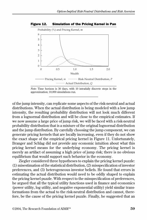
Option-Implied Risk-Neutral Distributions and Risk Aversion
©2004, The Research Foundation of AIMR™ 59
of the jump intensity, can replicate some aspects of the risk-neutral and actualdistributions. When the actual distribution is being modeled with a low jumpintensity, the resulting probability distribution will not look much differentfrom a lognormal distribution and will be close to the empirical estimates. Ifwe now assume a large price of jump risk, we will be faced with a risk-neutralprobability distribution that is a mixture of the original lognormal distributionand the jump distribution. By carefully choosing the jump component, we cangenerate pricing kernels that are locally increasing, even if they do not showthe exact shape of the empirical pricing kernel in Figure 11. Unfortunately,Branger and Schlag did not provide any economic intuition about what thispricing kernel means for the underlying economy. The pricing kernel ismerely an artifact of assuming a high price of jump risk; there is no obviousequilibrium that would support such behavior in the economy.
Ziegler considered three hypotheses to explain the pricing kernel puzzle:(1) misestimation of the statistical distribution, (2) misspecification of investorpreferences, and (3) heterogeneous investor beliefs. He found that errors inestimating the actual distribution would need to be oddly shaped to explainthe pricing kernel puzzle. With respect to the misspecification of preferences,he argued that all the typical utility functions used in finance and economics(power utility, log utility, and negative exponential utility) yield similar trans-formations from the actual to the risk-neutral distribution and cannot, there-fore, be the cause of the pricing kernel puzzle. Finally, he suggested that an
Figure 12. Simulation of the Pricing Kernel in Pan
Note: Time horizon is 30 days, with 10 intradaily discrete steps in theapproximation; 10,000 simulations run.
Probability (%) and Pricing Kernel, m
6
2
3
4
5
1
00 2.00.5 1.0 1.5
Wealth
Pricing Kernel, m Risk-Neutral Distribution, P
Actual Distribution, Q
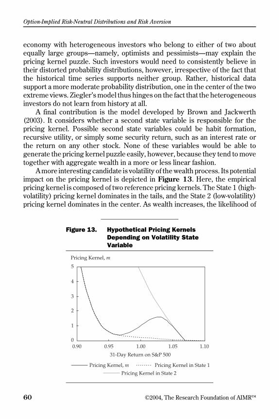
Option-Implied Risk-Neutral Distributions and Risk Aversion
60 ©2004, The Research Foundation of AIMR™
economy with heterogeneous investors who belong to either of two aboutequally large groups—namely, optimists and pessimists—may explain thepricing kernel puzzle. Such investors would need to consistently believe intheir distorted probability distributions, however, irrespective of the fact thatthe historical time series supports neither group. Rather, historical datasupport a more moderate probability distribution, one in the center of the twoextreme views. Ziegler’s model thus hinges on the fact that the heterogeneousinvestors do not learn from history at all.
A final contribution is the model developed by Brown and Jackwerth(2003). It considers whether a second state variable is responsible for thepricing kernel. Possible second state variables could be habit formation,recursive utility, or simply some security return, such as an interest rate orthe return on any other stock. None of these variables would be able togenerate the pricing kernel puzzle easily, however, because they tend to movetogether with aggregate wealth in a more or less linear fashion.
A more interesting candidate is volatility of the wealth process. Its potentialimpact on the pricing kernel is depicted in Figure 13. Here, the empiricalpricing kernel is composed of two reference pricing kernels. The State 1 (high-volatility) pricing kernel dominates in the tails, and the State 2 (low-volatility)pricing kernel dominates in the center. As wealth increases, the likelihood of
Figure 13. Hypothetical Pricing Kernels Depending on Volatility State Variable
Pricing Kernel, m
5
2
3
4
1
00.90 1.100.95 1.00 1.05
31-Day Return on S&P 500
Pricing Kernel, m Pricing Kernel in State 1
Pricing Kernel in State 2

Option-Implied Risk-Neutral Distributions and Risk Aversion
©2004, The Research Foundation of AIMR™ 61
being in State 2 first increases and then decreases again. Taking the expecta-tion over the volatility dimension yields the desired empirical pricing kernel,m. In combination, they can explain the pricing kernel puzzle because volatilitytends to be low in the center, where aggregate wealth does not change much.If wealth either increases or decreases rapidly, however, volatility shoots upand the result is a U-shaped profile of volatility as a function of wealth. Brownand Jackwerth (2003) modeled such an economy and were indeed able togenerate the pricing kernel puzzle, although it was smaller than what is shownin Figure 11. Figure 14 shows their pricing kernel.
Applications and Use. The research described in this final section iscertainly the least accessible in terms of using it in a practical context, but thematerial does have a number of applications. First, empirically plotting thepricing kernel puzzle for the index provides a measure of how much thevolatility smile is out of line with option prices that are consistent with risk-averse investors. With that information, some option prices can be consideredovervalued, and a gutsy trader can take advantage of that situation. Thisargument was made by Bondarenko (2002, 2003), Jackwerth (2000), andJones (2001). Selling out-of-the-money puts is the most obvious strategy tomake money out of overpriced portfolio insurance. This strategy entails largedownside risk, however, which many traders might not want to take or cannottake because of legal restrictions (even if such trades are utility increasing).
Figure 14. Simulated Pricing Kernel Based on Brown and Jackwerth
Pricing Kernel, m
1.10
1.00
1.05
0.95
0.900.90 1.100.95 1.00 1.05
31-Day Return on S&P 500
Option-Implied Risk-Neutral Distributions and Risk Aversion
62 ©2004, The Research Foundation of AIMR™
The strategy detailed in Jackwerth (2000), however, eliminates suchproblems. There, the most overpriced options are found to be actually thenear-the-money puts. The reason we do not see this fact in the implied volatilitychart is that, although the out-of-the-money puts are the most overvalued onesin relative terms, the near-the-money puts are more overvalued in absoluteterms. For a trading strategy, the absolute mispricing matters and a spread atwhich a trader sells the near-the-money puts and buys out-of-the-money puts(so the overall risk is comparable to being long the market) performs well.Because the out-of-the-money puts are so cheap in absolute terms, the traderis not compromising much of the profits. Although I do not know how thisstrategy will perform in the future, it performed well when historical data wereused, with an annualized excess return of 15–25 percent.
Driessen and Maenhout (2003) confirmed these results. In their study,they used the same strategy and also investigated selling at-the-money strad-dles (again, protected on the downside against market crashes by the purchaseof an out-of-the-money put). They found that these large profits are statisticallysignificant and robust to corrections for transaction costs, margin require-ments, and the “Peso Problem.”20 Even investors with nonexpected utilityfunctions (those with loss aversion or disappointment aversion or those whosuffer biases in decision making) would have found these trades desirable.21
Reasons for these profitable trades could lie either in investor irrationality,when investors pay more for portfolio insurance than they should; in a negative-volatility risk premium (Bakshi and Kapadia 2003; Coval and Shumway 2001);or in a positive jump risk premium (Bates 2001; Pan).
The discussion so far has focused on index options because the index isa large part of aggregate wealth in an economy. We can, however, look at thepricing kernel across some other variable—say, interest rates. In that case,we would need to use options on bonds to find the risk-neutral distributionand we would need to sample the historical time series of interest rates toobtain the actual distribution. The pricing kernel will then be the projectionof the economywide pricing kernel (which is normally defined across aggre-gate wealth) onto the space of interest rates. Because the correlation betweeninterest rates and aggregate wealth is typically low, the pricing kernel at anygiven interest rate level will be an average of the pricing kernel levels acrossaggregate wealth; that is, it will be almost constant at the price of a unitdiscount bond.
20The Peso Problem is when a rare event (e.g., a high-interest rate regime or a market crash)occurs less frequently in the sample data than is rationally anticipated.21These utility functions are described in behavioral finance and model investors who careabout losses and gains with respect to a reference point (such as last period’s wealth) asopposed to aggregate wealth (or consumption) or investors who consistently misestimate theprobabilities of very rare or very likely events.
Option-Implied Risk-Neutral Distributions and Risk Aversion
©2004, The Research Foundation of AIMR™ 63
Empirically, we can then measure flat pricing kernels that are just belowa level of 1 when the state variable is not highly correlated with aggregatewealth. A downward-sloping pricing kernel would be a sign of high positivecorrelation with aggregate wealth, and an upward-sloping pricing kernelwould indicate state variables that can serve as a hedge because they moveagainst movements in aggregate wealth. We could even track the time seriesof these pricing kernels to learn how much interest rates, for example, movetogether with aggregate wealth in the eyes of the market.
In conclusion, this discussion has shown that a triangular relationshipexists between risk-neutral probabilities, actual probabilities, and the scaledmarginal utility (pricing kernel). Given any two quantities, we can infer thethird. Historically, the path taken was to assume a model for the actualprobabilities and a utility function for the representative agent (or a dynami-cally complete market, in which case we can mathematically determine theassociated pricing kernel and thereby the utility function). Then, we derivedthe risk-neutral probabilities and priced all the securities. Based on thissection, this view has been turned upside down: We can estimate the risk-neutral and actual probability distributions to estimate the implied utilityfunctions, which are notoriously difficult to observe.
OutlookThe crash of 1987 was a dramatic experience for the stock market. It alsochanged the patterns in the options markets literally from one day to the next.Whereas before the crash the implied volatility smile was largely flat andbroadly consistent with Black–Scholes option prices, after the crash it becameseverely skewed, especially in the index option markets. As a result, mucheffort has been exerted to develop new parametric option-pricing models—namely, by incorporating additional stochastic factors, such as stochasticjumps, stochastic volatility, and stochastic interest rates.
A second line of research has been devoted to analyzing the observedoption prices and using the implied information to price other options. Theresults are methods that recover the risk-neutral probability distribution fromsets of option prices with common times to expiration. Once these tools becameavailable, they were soon applied to a variety of questions in addition to pricingexotic options—for example, for investigating the impact of news on probabilityassessments and for forecasting. Naturally, interest has risen in learning moreabout the stochastic process that leads up to such terminal distribution, andimplied binomial trees do provide exactly this information. Unfortunately, theworld is not quite as simple as a model that we can fit to an implied volatilitysurface once and leave unchanged over time. Rather, the implied volatilitysurfaces evolve as a stochastic process, which needs to be modeled.
Option-Implied Risk-Neutral Distributions and Risk Aversion
64 ©2004, The Research Foundation of AIMR™
Risk-neutral probabilities in conjunction with actual probabilities also tellus about implied utility functions and thus about the economywide prefer-ences that investors exhibit. This information provides a fascinating look atthe economy.
Finally, I would like to speculate a bit about the future of this area offinancial economics. The analysis of option-implied risk-neutral distributionsis now a mature field, and it is here to stay. But questions are still open toinvestigation in the area of assessing the quality of these distributions, andonce the effort is made to understand the cross-sectional error structure ofoption prices, the future will provide the necessary statistical tests. Impliedbinomial trees have faded in interest recently, because they are complicatedto handle and cannot forecast option prices well. The other parametric option-pricing models also do not forecast option prices well, but because they arealready around and being used, practitioners are showing little inclination tomove to implied binomial trees. As always, the best option-pricing model willmost likely turn out to be some mixed model that has parametric aspects aswell as implied-tree aspects that incorporate observed market prices. TheHeath–Jarrow–Morton model for interest rates might well point the way forequity option pricing.
A clear understanding of the pricing kernel puzzle will come only in time.Is it the result of widespread mispricing in the most liquid option marketsacross the world, or is it explainable within standard economic reasoning? Themost important future developments lie in finding an improved understandingof how to move from risk-neutral to actual distributions, especially for securi-ties that are correlated with aggregate wealth but not perfectly so. Forecastingand risk management will be much easier when research developments allowus to use the risk-neutral distributions even more than we do right now.
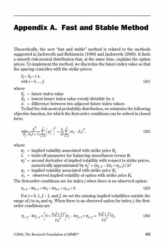
©2004, The Research Foundation of AIMR™ 65
Appendix A. Fast and Stable Method
Theoretically, the new “fast and stable” method is related to the methodssuggested in Jackwerth and Rubinstein (1996) and Jackwerth (2000). It findsa smooth risk-neutral distribution that, at the same time, explains the optionprices. To implement the method, we discretize the future index value so thatthe spacing coincides with the strike prices:
Sj = S0 + j ∆,with j = 0,…, J, (A1)
whereSj = future index valueS0 = lowest future index value evenly divisible by ∆∆ = difference between two adjacent future index valuesTo find the risk-neutral probability distribution, we minimize the following
objective function, for which the first-order conditions can be solved in closedform:
(A2)
whereσj = implied volatility associated with strike price Kjλ = trade-off parameter for balancing smoothness versus fitσj″ = second derivative of implied volatility with respect to strike prices,
numerically approximated by σj″ = (σj–1 – 2σj + σj+1)/∆2
σi = implied volatility associated with strike price Ki= observed implied volatility of option with strike price Ki
The first-order conditions are for index j when there is no observed option:
σj–2 – 4σj–1 + 6σj – 4σj+1 + σj+2 = 0. (A3)
For j = 0, 1, J – 1, and J, we set the missing implied volatilities outside therange of j to σ0 and σJ. When there is an observed option for index j, the first-order conditions are
(A4)
minσj
∆4
2 J 1+( )------------------- σ″j⎝ ⎠
⎛ ⎞2 λ
2I----- σi σi–( )
2,
i 1=
I
∑+j 0=
J
∑
σi
σj 2– 4σj 1–– 6 λ J 1+( )
I∆4-------------------+ σj 4σj 1+– σj 2++ +
λ J 1+( )
I∆4-------------------σj.=
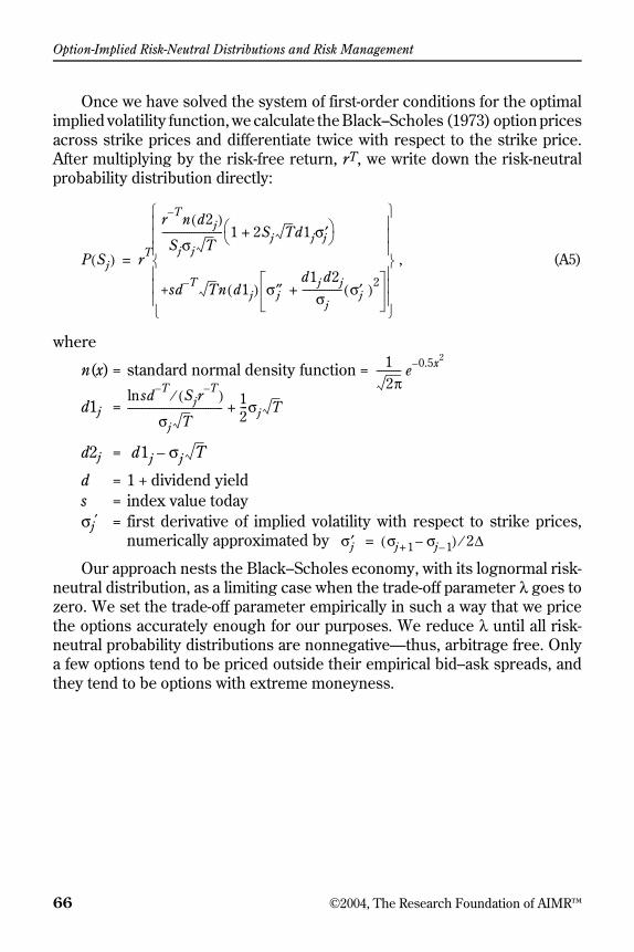
Option-Implied Risk-Neutral Distributions and Risk Management
66 ©2004, The Research Foundation of AIMR™
Once we have solved the system of first-order conditions for the optimalimplied volatility function, we calculate the Black–Scholes (1973) option pricesacross strike prices and differentiate twice with respect to the strike price.After multiplying by the risk-free return, rT, we write down the risk-neutralprobability distribution directly:
(A5)
where
n(x) = standard normal density function =
d1j =
d2j =
d = 1 + dividend yields = index value todayσj′ = first derivative of implied volatility with respect to strike prices,
numerically approximated by
Our approach nests the Black–Scholes economy, with its lognormal risk-neutral distribution, as a limiting case when the trade-off parameter λ goes tozero. We set the trade-off parameter empirically in such a way that we pricethe options accurately enough for our purposes. We reduce λ until all risk-neutral probability distributions are nonnegative—thus, arbitrage free. Onlya few options tend to be priced outside their empirical bid–ask spreads, andthey tend to be options with extreme moneyness.
P Sj( ) rT
r T– n d2j( )
Sjσj T------------------------- 1 2Sj Td1jσ′j+⎝ ⎠
⎛ ⎞
+sd T– Tn d1j( ) σ″jd1j d2j
σj---------------- σj′( )2
+
⎩ ⎭⎪ ⎪⎪ ⎪⎪ ⎪⎨ ⎬⎪ ⎪⎪ ⎪⎪ ⎪⎧ ⎫
,=
12π
---------- e 0.5x2–
sd T– SjrT–( )⁄ln
σj T---------------------------------------
12---σj T+
d1j σj T–
σ′j σj 1+ σj 1––( ) 2∆⁄=
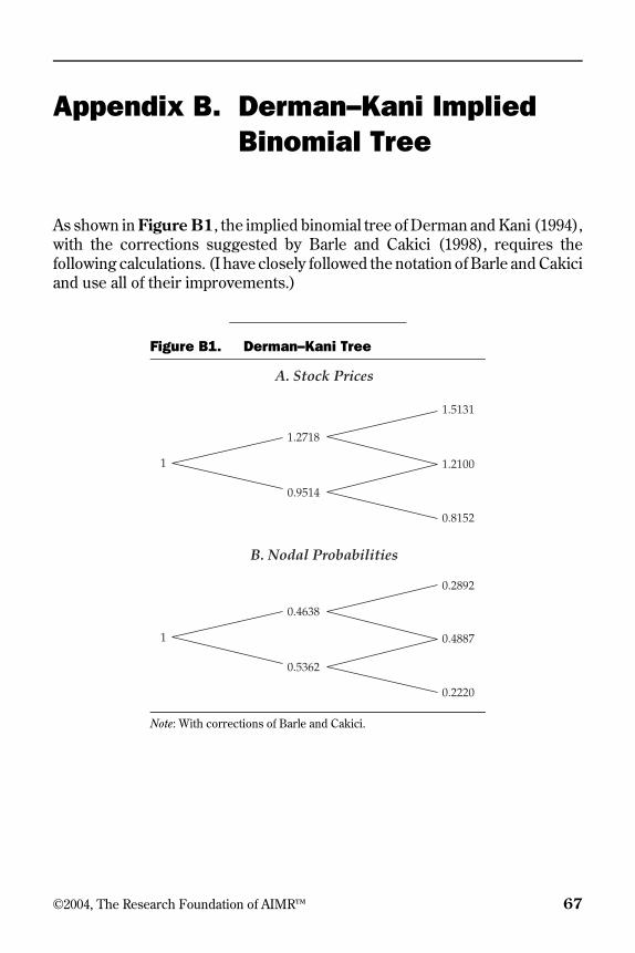
©2004, The Research Foundation of AIMR™ 67
Appendix B. Derman–Kani Implied Binomial Tree
As shown in Figure B1, the implied binomial tree of Derman and Kani (1994),with the corrections suggested by Barle and Cakici (1998), requires thefollowing calculations. (I have closely followed the notation of Barle and Cakiciand use all of their improvements.)
Figure B1. Derman–Kani Tree
Note: With corrections of Barle and Cakici.
0.2892
0.4638
1
0.5362
0.4887
0.2220
1.5131
1.2718
1
0.9514
1.2100
0.8152
A. Stock Prices
B. Nodal Probabilities

Option-Implied Risk-Neutral Distributions and Risk Management
68 ©2004, The Research Foundation of AIMR™
The lower intermediate stock price follows from (with i = 1):
where
Fi = Si (r/d)∆t = 1.1 Si = today’s stock price ∆t = one time-step of one year λi = the state-contingent price today (= 1)
C(Fi, tn+1) = 0.0724 = the call expiring next period with strike price Fi
The upper intermediate stock price follows from Si+1 = = 1.21/0.9514 =1.2718. The upper intermediate probability can then be derived from
and the lower intermediate probability is 1 – 0.4638 = 0.5362.To construct the terminal step, we start with the center node:
where n = 2.
Si FiλiFi ∆i
C–
λiFi ∆iC
+-------------------------=
1.11 1.1( ) 0.0797–1 1.1( ) 0.0797+--------------------------------------=
0.9514,=
∆iC r∆tC Fi, t n 1+( ) λj Fj Fi–( )
j i 1+=
n
∑–=
F i2 Si⁄
piFi Si–
Si 1+ Si–---------------------=
1.1 0.9514–1.2718 0.9514–---------------------------------------=
0.4638,=
S n 2⁄( ) 1+ S1rd---⎝ ⎠
⎛ ⎞tn 1+
=
1.12=
1.21,=
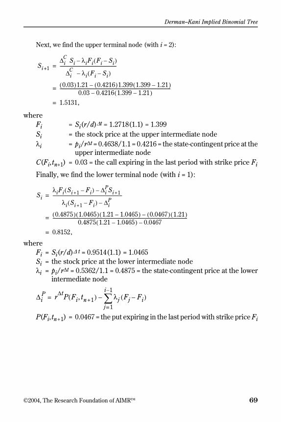
Derman–Kani Implied Binomial Tree
©2004, The Research Foundation of AIMR™ 69
Next, we find the upper terminal node (with i = 2):
where Fi = Si(r/d)∆t = 1.2718(1.1) = 1.399Si = the stock price at the upper intermediate nodeλi = pi/r∆t = 0.4638/1.1 = 0.4216 = the state-contingent price at the
upper intermediate nodeC(Fi,tn+1) = 0.03 = the call expiring in the last period with strike price Fi
Finally, we find the lower terminal node (with i = 1):
where Fi = Si(r/d)∆ t = 0.9514(1.1) = 1.0465Si = the stock price at the lower intermediate nodeλi = pi/r∆t = 0.5362/1.1 = 0.4875 = the state-contingent price at the lower
intermediate node
P(Fi, tn+1) = 0.0467 = the put expiring in the last period with strike price Fi
Si 1+
∆iC Si λiFi Fi Si–( )–
∆iC λi Fi Si–( )–
----------------------------------------------------=
0.03( )1.21 0.4216( )1.399 1.399 1.21–( )–0.03 0.4216 1.399 1.21–( )–
------------------------------------------------------------------------------------------------------=
1.5131,=
SiλiFi Si +1 Fi–( ) ∆i
PSi +1–
λi Si +1 Fi–( ) ∆iP–
----------------------------------------------------------------=
0.4875( ) 1.0465( ) 1.21 1.0465–( ) 0.0467( ) 1.21( )–0.4875 1.21 1.0465–( ) 0.0467–
----------------------------------------------------------------------------------------------------------------------------=
0.8152,=
∆iP r∆tP Fi, tn +1( ) λj Fj Fi–( )
j 1=
i 1–
∑–=
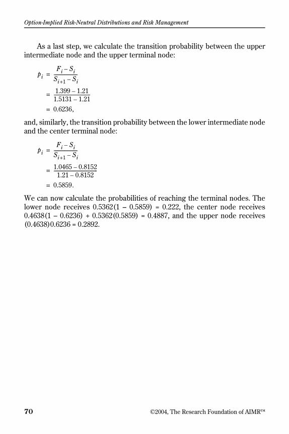
Option-Implied Risk-Neutral Distributions and Risk Management
70 ©2004, The Research Foundation of AIMR™
As a last step, we calculate the transition probability between the upperintermediate node and the upper terminal node:
and, similarly, the transition probability between the lower intermediate nodeand the center terminal node:
We can now calculate the probabilities of reaching the terminal nodes. Thelower node receives 0.5362(1 – 0.5859) = 0.222, the center node receives0.4638(1 – 0.6236) + 0.5362(0.5859) = 0.4887, and the upper node receives(0.4638)0.6236 = 0.2892.
piFi Si–
Si 1+ Si–---------------------=
1.399 1.21–1.5131 1.21–---------------------------------=
0.6236,=
piFi Si–
Si 1+ Si–---------------------=
1.0465 0.8152–1.21 0.8152–
---------------------------------------=
0.5859.=

©2004, The Research Foundation of AIMR™ 71
Glossary
AMERICAN OPTION: An option that can be exercised at any time on or before theexpiration date.
AT-THE-MONEY CALL: A call with a strike price equal to (or very near) the market priceof the underlying security.
BETA FUNCTION OF THE SECOND KIND: A generalization of the beta density function,first suggested by Bookstaber and McDonald (1987).
BID–ASK SPREAD: The difference between the current bid price (price at which aninvestor can sell) and the current ask price (price at which an investor can buy) for agiven security.
BINOMIAL TREE: A graphical representation of a binomial model showing the possibleoutcomes or states associated with an option and its underlying asset. The underlyingasset can only move up or down over each time step.
BROWNIAN MOTION: A continuous-time STOCHASTIC process with independent incre-ments that have a normal distribution with mean 0 and variance 1 per unit of time.
BURR-TYPE DISTRIBUTION: A class of 12 cumulative distribution functions suggestedby Burr (1942).
CALL OPTION: The right, but not the obligation, to buy a particular asset at a specifiedprice within a specified period of time.
COMPLETE MARKET: A market in which all future payoffs on future states of the worldcan be constructed with existing assets.
CONFLUENT HYPERGEOMETRIC FUNCTION: A degenerate form of the hypergeometricfunction that arises as a solution to the confluent hypergeometric differential equation.
DELTA: See OPTION DELTA.
DIFFUSION PROCESS: A process—for example, of the logarithm of stock prices—thatincreases at each instant of time (drifts) and also changes randomly up or down (thediffusion term) based on a BROWNIAN MOTION.
EDGEWORTH EXPANSION: An ordering of GRAM–CHARLIER EXPANSIONS by collectingterms of equal order.
ENTROPY: A measure of distance between probabilities.
EQUITY RISK PREMIUM: The extra return that the overall stock market or a particularstock must provide over the risk-free rate to compensate for market risk.
EUROPEAN OPTION: An option that can be exercised only on the expiration date.
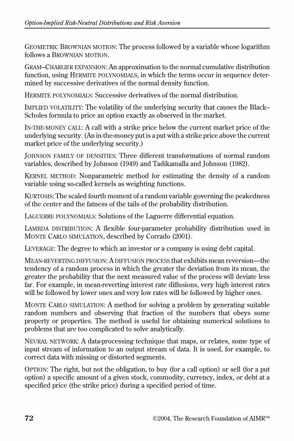
Option-Implied Risk-Neutral Distributions and Risk Aversion
72 ©2004, The Research Foundation of AIMR™
GEOMETRIC BROWNIAN MOTION: The process followed by a variable whose logarithmfollows a BROWNIAN MOTION.
GRAM–CHARLIER EXPANSION: An approximation to the normal cumulative distributionfunction, using HERMITE POLYNOMIALS, in which the terms occur in sequence deter-mined by successive derivatives of the normal density function.
HERMITE POLYNOMIALS: Successive derivatives of the normal distribution.
IMPLIED VOLATILITY: The volatility of the underlying security that causes the Black–Scholes formula to price an option exactly as observed in the market.
IN-THE-MONEY CALL: A call with a strike price below the current market price of theunderlying security. (An in-the-money put is a put with a strike price above the currentmarket price of the underlying security.)
JOHNSON FAMILY OF DENSITIES: Three different transformations of normal randomvariables, described by Johnson (1949) and Tadikamalla and Johnson (1982).
KERNEL METHOD: Nonparametric method for estimating the density of a randomvariable using so-called kernels as weighting functions.
KURTOSIS: The scaled fourth moment of a random variable governing the peakednessof the center and the fatness of the tails of the probability distribution.
LAGUERRE POLYNOMIALS: Solutions of the Laguerre differential equation.
LAMBDA DISTRIBUTION: A flexible four-parameter probability distribution used inMONTE CARLO SIMULATION, described by Corrado (2001).
LEVERAGE: The degree to which an investor or a company is using debt capital.
MEAN-REVERTING DIFFUSION: A DIFFUSION PROCESS that exhibits mean reversion—thetendency of a random process in which the greater the deviation from its mean, thegreater the probability that the next measured value of the process will deviate lessfar. For example, in mean-reverting interest rate diffusions, very high interest rateswill be followed by lower ones and very low rates will be followed by higher ones.
MONTE CARLO SIMULATION: A method for solving a problem by generating suitablerandom numbers and observing that fraction of the numbers that obeys someproperty or properties. The method is useful for obtaining numerical solutions toproblems that are too complicated to solve analytically.
NEURAL NETWORK: A data-processing technique that maps, or relates, some type ofinput stream of information to an output stream of data. It is used, for example, tocorrect data with missing or distorted segments.
OPTION: The right, but not the obligation, to buy (for a call option) or sell (for a putoption) a specific amount of a given stock, commodity, currency, index, or debt at aspecified price (the strike price) during a specified period of time.
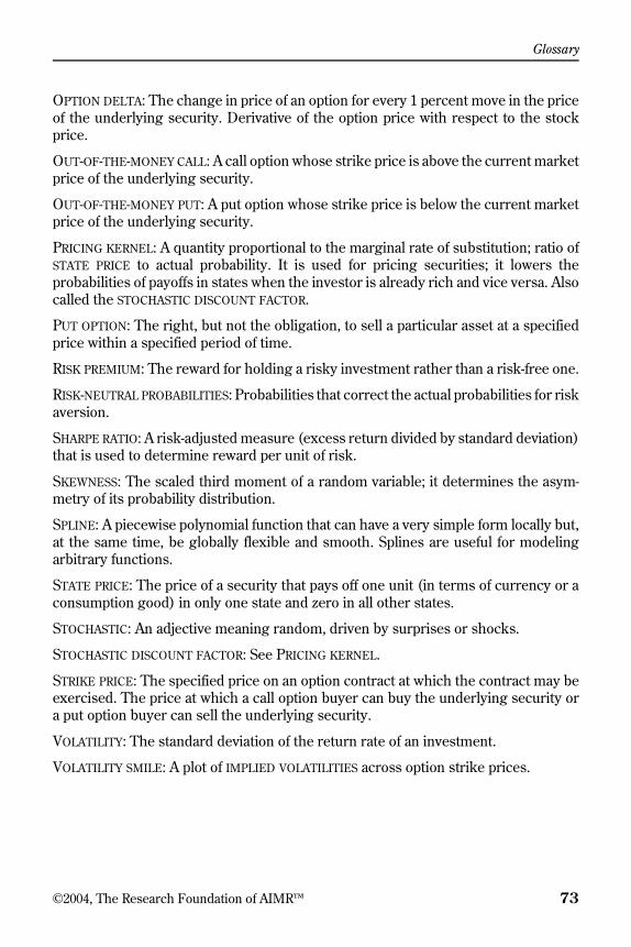
Glossary
©2004, The Research Foundation of AIMR™ 73
OPTION DELTA: The change in price of an option for every 1 percent move in the priceof the underlying security. Derivative of the option price with respect to the stockprice.
OUT-OF-THE-MONEY CALL: A call option whose strike price is above the current marketprice of the underlying security.
OUT-OF-THE-MONEY PUT: A put option whose strike price is below the current marketprice of the underlying security.
PRICING KERNEL: A quantity proportional to the marginal rate of substitution; ratio ofSTATE PRICE to actual probability. It is used for pricing securities; it lowers theprobabilities of payoffs in states when the investor is already rich and vice versa. Alsocalled the STOCHASTIC DISCOUNT FACTOR.
PUT OPTION: The right, but not the obligation, to sell a particular asset at a specifiedprice within a specified period of time.
RISK PREMIUM: The reward for holding a risky investment rather than a risk-free one.
RISK-NEUTRAL PROBABILITIES: Probabilities that correct the actual probabilities for riskaversion.
SHARPE RATIO: A risk-adjusted measure (excess return divided by standard deviation)that is used to determine reward per unit of risk.
SKEWNESS: The scaled third moment of a random variable; it determines the asym-metry of its probability distribution.
SPLINE: A piecewise polynomial function that can have a very simple form locally but,at the same time, be globally flexible and smooth. Splines are useful for modelingarbitrary functions.
STATE PRICE: The price of a security that pays off one unit (in terms of currency or aconsumption good) in only one state and zero in all other states.
STOCHASTIC: An adjective meaning random, driven by surprises or shocks.
STOCHASTIC DISCOUNT FACTOR: See PRICING KERNEL.
STRIKE PRICE: The specified price on an option contract at which the contract may beexercised. The price at which a call option buyer can buy the underlying security ora put option buyer can sell the underlying security.
VOLATILITY: The standard deviation of the return rate of an investment.
VOLATILITY SMILE: A plot of IMPLIED VOLATILITIES across option strike prices.
74 ©2004, The Research Foundation of AIMR™
References
Abadir, K., and M. Rockinger. 1997. “Density-Embedding Functions.” Workingpaper, HEC.
Abken, P., D. Madan, and S. Ramamurtie. 1996a. “Estimation of Risk-Neutral and Sta-tistical Densities by Hermite Polynomial Approximation: With an Application to Euro-dollar Futures Options.” Working paper, Federal Reserve Bank of Atlanta.
———. 1996b. “Pricing S&P 500 Index Options Using a Hilbert Space Basis.” Work-ing paper, Federal Reserve Bank of Atlanta.
Aït-Sahalia, Y., and A. Lo. 1998. “Nonparametric Estimation of State-Price DensitiesImplicit in Financial Asset Prices.” Journal of Finance, vol. 53, no. 2 (April):499–547.
———. 2000. “Nonparametric Risk Management and Implied Risk Aversion.” Jour-nal of Econometrics, vol. 94, nos. 1–2 (January/February):9–51.
Alexander, C. 2001. “Principal Component Analysis of Implied Volatility Smiles andSkews.” Working paper, University of Reading.
Amerio, E., G. Fusai, and A. Vulcano. 2001. “Price of Implied Volatility Derivatives: ARisk Neutral Model for Market Implied Volatility.” Working paper, INSEAD.
Anagnou, I., M. Bedendo, S. Hodges, and R. Tompkins. 2002. “The Relation betweenImplied and Realized Probability Density Functions.” Working paper, University ofWarwick.
Andersen, A., and T. Wagener. 2002. “Extracting Risk Neutral Probability Densitiesby Fitting Implied Volatility Smiles: Some Methodological Points and an Applicationto the 3M EURIBOR Futures Option Prices.” Working paper, European Central Bank.
Andersen, L., and R. Brotherson-Ratcliffe. 1997. “The Equity Option Volatility Smile:An Implicit Finite Difference Approach.” Journal of Computational Finance, vol. 1,no. 2 (Winter):5–38.
Aparicio, S., and S. Hodges. 1998. “Implied Risk-Neutral Distribution: A Comparisonof Estimation Methods.” Working paper, Warwick University.
Avellaneda, M., C. Friedman, R. Holmes, and D. Samperi. 1997. “Calibrating VolatilitySurfaces via Relative-Entropy Minimization.” Applied Mathematical Finance, vol. 4,no. 1 (March):37–64.
Bachelier, L. 1900. “Theorie de la Speculation,” Annales de l’Ecole NormaleSuperieure, vol. 17.
Bahra, B. 1997. “Implied Risk-Neutral Probability Density Functions from OptionPrices: Theory and Application.” Working paper, Bank of England.
Bakshi, G., and N. Kapadia. 2003. “Delta-Hedged Gains and the Negative Market Vol-atility Risk Premium.” Review of Financial Studies, vol. 16, no. 2 (Summer):527–566.

References
©2004, The Research Foundation of AIMR™ 75
Bakshi, G., C. Cao, and Z. Chen. 1997. “Empirical Performance of Alternative OptionPricing Models.” Journal of Finance, vol. 52, no. 5 (December):2003–49.
Banz, R., and M. Miller. 1978. “Prices for State-Contingent Claims: Some Estimatesand Applications.” Journal of Business, vol. 51, no. 4 (October):653–672.
Barle, S., and N. Cakici. 1998. “How to Grow a Smiling Tree.” Journal of FinancialEngineering, vol. 7, no. 2 (June):127–146.
Barone-Adesi G., and R. Whaley. 1987. “Efficient Analytic Approximation of AmericanOption Values.” Journal of Finance, vol. 42, no. 2 (June):301–320.
Bartunek, K., and M. Chowdhury. 1997. “Implied Risk Aversion Parameters fromOption Prices.” Financial Review, vol. 32, no. 1 (February):107–124.
Bates, D. 1991. “The Crash of ‘87: Was It Expected? The Evidence from Options Mar-kets.” Journal of Finance, vol. 46, no. 3 (July):1009–44.
———. 1996. “Jumps and Stochastic Volatility: Exchange Rate Processes Implicit inDeutsche Mark Options.” Review of Financial Studies, vol. 9, no. 1 (Spring):69–107.
———. 2000. “Post-’87 Crash Fears in S&P 500 Futures Options.” Journal of Econo-metrics, vol. 94, nos. 1–2 (January/February):181–238.
———. 2001. “The Market for Crash Risk.” Working Paper No. 8557, NationalBureau of Economic Research, Cambridge, MA.
Beber, A. 2001. “Determinants of the Implied Volatility Function of the Italian StockMarket.” Working paper, University of Pennsylvania.
Beber, A., and M. Brandt. 2003. “The Effect of Macroeconomic News on Beliefs andPreferences: Evidence from the Options Market.” Working paper, St. Anna School ofAdvanced Studies.
Benhamou, E. 2003. “Options, Pre-Black Scholes.” Working paper, Goldman Sachs.
Benninga, S., and J. Mayshar. 1997. “Heterogeneity and Option Pricing.” Workingpaper, University of Pennsylvania.
Berkowitz, J. 2001. “Getting the Right Option Price with the Wrong Model.” Workingpaper, University of California at Irvine.
Bernardo, A., and O. Ledoit. 2000. “Gain, Loss and Asset Pricing.” Journal of PoliticalEconomy, vol. 108, no. 1 (February):173–206.
Black, F. 1976. “Studies of Stock Price Volatility Changes.” Proceedings of the 1976Meetings of the American Statistical Association, Business and Economical StatisticsSection:177–181.
Black, F., and M. Scholes. 1973. “Pricing of Options and Corporate Liabilities.” Jour-nal of Political Economy, vol. 81, no. 3 (May/June):637–659.
Blair, B., S-H Poon, and S. Taylor. 2001. “Forecasting S&P 100 Volatility: The Incre-mental Information Content of Implied Volatilities and High Frequency IndexReturns.” Journal of Econometrics, vol. 105, no. 1 (November):5–26.

Option-Implied Risk-Neutral Distributions and Risk Aversion
76 ©2003, The Research Foundation of AIMR™
Bliss, R., and N. Panigirtzoglou. 2001. “Testing the Stability of Implied ProbabilityDensity Functions.” Journal of Banking and Finance, vol. 26, no. 2–3 (March):381–422.
———. 2002. “Option-Implied Risk Aversion Estimates: Robustness and Patterns.”Previously titled: “Recovering Risk Aversion from Options.” Working paper, FederalReserve Bank of Chicago.
Bodurtha, J., and M. Jermakyan. 1996a. “Non-Parametric Estimation of an ImpliedVolatility Surface.” Working paper, Georgetown University.
———. 1996b. “Regular Smiles.” Working paper, Georgetown University.
Bollen, N., and E. Rasiel. 2002. “The Performance of Alternative Valuation Models inthe OTC Currency Options Market.” Working paper, Vanderbilt University.
Bollen, N. and R. Whaley. 2001. “What Determines the Shape of Implied VolatilityFunctions?” Working paper, Vanderbilt University.
Bondarenko, O. 2000. “Recovering Risk-Neutral Densities: A New NonparametricApproach.” Working paper, University of Illinois.
———. 2002. “Why Are Puts So Expensive?” Working paper, University of Illinois.
———. 2003. “Statistical Arbitrage and Security Prices.” Review of Financial Studies,vol. 16, no. 3 (Fall):875–919.
Boness, A. 1964. “Elements of a Theory of Stock-Option Valuation.” Journal of Politi-cal Economy, vol. 72, no. 2 (April):163–175.
Bookstaber, R., and J. McDonald. 1987. “A General Distribution for Describing Secu-rity Price Returns.” Journal of Business, vol. 60, no. 3 (July):401–424.
Bouchouev, I., and V. Isakov. 1997. “The Inverse Problem of Option Pricing.” InverseProblems, vol. 13, no. 5 (October):L11–L17.
Branger, N. 2002. “Pricing Derivative Securities using Cross-Entropy: An EconomicAnalysis.” Working paper, School of Business and Economics, Goethe University.
Branger, N., and C. Schlag. 2002. “Why Is the Index Smile So Steep?” Working paper,University of Frankfurt.
Breeden, D., and R. Litzenberger. 1978. “Prices of State-Contingent Claims Implicitin Options Prices.” Journal of Business, vol. 51, no. 4 (October):621–651.
Brenner, M., and Y. Eom. 1997. “No-Arbitrage Option Pricing: New Evidence on theValidity of the Martingale Property.” Working paper, New York University.
Brenner, M., Y. Eom, and Y. Landskroner. 1996. “Implied Foreign Exchange Rates Us-ing Options Prices.” International Review of Financial Analysis, vol. 5, no. 3:171–183.
Brigo, D., and F. Mercurio. 2002. “Lognormal-Mixture Dynamics and Calibration toVolatility Smiles and Skews.” International Journal of Theoretical and AppliedFinance, vol. 5, no. 4 (June):427–446.
Britten-Jones, M., and A. Neuberger. 2000. “Option Prices, Implied Price Processes,and Stochastic Volatility.” Journal of Finance, vol. 55, no. 2 (April):839–866.
References
©2004, The Research Foundation of AIMR™ 77
Brown, D., and J. Jackwerth. 2000. “The Information Content of the Volatility Smile.”Working paper, University of Wisconsin at Madison.
———. 2003. “The Kernel Pricing: Reconciling Index Option Data and EconomicTheory.” Working paper, University of Wisconsin at Madison.
Brown, G., and K. Toft. 1999. “Constructing Binomial Trees from Multiple ImpliedProbability Distributions.” Journal of Derivatives, vol. 7, no. 2 (Winter):83–100.
Buchen, P., and M. Kelly. 1996. “The Maximum Entropy Distribution of an Asset In-ferred from Option Prices.” Journal of Financial and Quantitative Analysis, vol. 31,no. 1 (March):143–159.
Buraschi, A., and J. Jackwerth. 2001. “The Price of a Smile: Hedging and Spanning inOption Markets.” Review of Financial Studies, vol. 14, no. 2 (Summer):495–527.
Burr, I. 1942. “Cumulative Frequency Functions.” Annals of Mathematical Statistics,vol. 13:627–635.
Campa, J., and K. Chang. 1996. “Arbitrage-Based Tests of Target Zone Credibility:Evidence from ERM Cross-Rate Options.” American Economic Review, vol. 86, no. 4(September):726–740.
———. 1998. “ERM Realignment Risk and its Economic Determinants as Reflectedin Cross-Rate Options.” Economic Journal, vol. 108, no. 449 (July):1046–66.
Campa, J., K. Chang, and J. Refalo. 1999. “An Options-Based Analysis of EmergingMarket Exchange Rate Expectations: Brazil’s Real Plan, 1994–1999.” Working paper,New York University.
Campa, J., K. Chang, and R. Reider. 1998. “Implied Exchange Rate Distributions: Evi-dence from OTC Option Markets.” Journal of International Money and Finance, vol.17, no. 1 (February):117–160.
Campbell, J., and J. Cochrane. 2000. “Explaining the Poor Performance of Consump-tion-Based Asset Pricing Models.” Journal of Finance, vol. 55, no. 6 (December):2863–78.
Campbell, J., and L. Hentschel. 1992. “No News Is Good News: An Asymmetric Mod-el of Changing Volatility in Stock Returns.” Journal of Financial Economics, vol. 31,no. 3 (June):281–318.
Campbell, R., K. Koedijk, and P. Kofman. 2002. “Increased Correlation in Bear Mar-kets: A Downside Risk Perspective.” Discussion Paper 3172, Centre for EconomicPolicy Research.
Carr, P., and D. Madan. 2001. “Determining Volatility Surfaces and Option Valuesfrom an Implied Volatility Smile.” In Quantitative Analysis in Financial Markets, vol.11. Edited by M. Avellaneda. Singapore and River Edge, NJ: World Scientific.
Carr, P., M. Tari, and T. Zariphopoulou. 1999. “Closed Form Option Valuation withSmiles.” Working paper, Bank of America Securities and University of Texas at Austin.
Option-Implied Risk-Neutral Distributions and Risk Aversion
78 ©2003, The Research Foundation of AIMR™
Carverhill, A., and S. Dyrting. 2000. “The Information Content of Implied Volatility forCME Japanese Yen and S&P 500 Futures Options.” Working paper, University of Sci-ence and Technology, Hong Kong.
Chernov, M. 2000. “A Case of Empirical Reverse Engineering: Estimation of the Pric-ing Kernel.” Working paper, Pennsylvania State University.
Chriss, N. 1996. “Transatlantic Trees.” Risk, vol. 9, no. 7 (September):46–49.
Christensen, B., and N. Prabhala. 1998. “The Relation between Implied and RealizedVolatility.” Journal of Financial Economics, vol. 50, no. 2 (November):125–150.
Christie, A. 1982. “The Stochastic Behavior of Common Stock Variance—Value,Leverage and Interest Rate Effects.” Journal of Financial Economics, vol. 10, no. 4(December):407–432.
Christoffersen, P., and K. Jacobs. 2001. “The Importance of the Loss Function inOption Pricing.” Working paper, McGill University.
Clark, I. 2002. “Feasible Volatility Smiles and Their Implied Probability Distributionsfor Asset Prices.” Working paper, BNP Paribas.
Clews, R., N. Panigirtzoglou, and J. Proudman. 2000. “Recent Developments inExtracting Information from Options Markets.” Bank of England Quarterly Bulletin(February):50–60.
Cochrane, J., and J. Saa-Requejo. 2000. “Beyond Arbitrage: Good-Deal Asset PriceBounds in Incomplete Markets.” Journal of Political Economy, vol. 108, no. 1(February):79–119.
Coleman, T., Y. Li, and A. Verma. 1999. “Reconstructing the Unknown VolatilityFunction.” Journal of Computational Finance, vol. 2, no. 3 (Spring):77–102.
Constantinides, G., and S. Perrakis. 2002. “Stochastic Dominance Bounds on Deriva-tives Prices in a Multiperiod Economy with Proportional Transaction Costs.” Journalof Economic Dynamics and Control, vol. 26, no. 7–8 (July):1323–52.
Cont, R. 1997. “Beyond Implied Volatility.” In Econophysics. Edited by J. Kertesz andI. Kondor. Dordrecht, Netherlands: Kluwer.
Cont, R, and J. da Fonseca. 2002. “Dynamics of Implied Volatility Surfaces.” Quanti-tative Finance, vol. 2, no. 1 (February):45–60.
Cont, R., J. da Fonseca, and V. Durrleman. 2002. “Stochastic Models of Implied Vola-tility Surfaces.” Economic Notes, vol. 31, no. 2 (July):361–377.
Cooper, N. 1999. “Testing Techniques for Estimating Implied RNDs from the Pricesof European-Style Options.” Working paper, Bank of England.
Corrado, C. 2001. “Option Pricing Based on the Generalized Lambda Distribution.”Journal of Futures Markets, vol. 21, no. 3 (March):213–236.
References
©2004, The Research Foundation of AIMR™ 79
Corrado, C., and T. Su. 1996. “Skewness and Kurtosis in S&P 500 Index ReturnsImplied by Option Prices.” Journal of Financial Research, vol. 19, no. 2 (Summer):175–192.
———. 1997. “Implied Volatility Skews and Stock Index Skewness and KurtosisImplied by S&P 500 Index Option Prices.” Journal of Derivatives, vol. 4, no. 4 (Sum-mer):8–19.
Coutant, S. 2000. “Time-Varying Implied Risk Aversion in Options Prices Using Her-mite Polynomials.” Working paper, Banque de France.
Coutant, S., E. Jondeau, and M. Rockinger. 2001. “Reading PIBOR Futures Options’Smiles: The 1997 Snap Election.” Journal of Banking and Finance, vol. 25, no. 11(November): 1957–87.
Coval, J., and T. Shumway. 2001. “Expected Option Returns.” Journal of Finance, vol.56, no. 3 (June):983–1009.
Cox, J., S. Ross, and M. Rubinstein. 1979. “Option Pricing: A Simplified Approach.”Journal of Financial Economics, vol. 7, no. 3 (September):229–263.
Degoeij, P., and W. Marquering. 2002. “Do Macroeconomic Announcements CauseAsymmetric Volatility?” Working paper, University of Leuven.
De Jong, C., and T. Lehnert. 2001. “Implied Garch Volatility Forecasting.” Workingpaper, Erasmus University.
De Jong, C., and R. Huisman. 2000. “From Skews to a Skewed-t: Modelling Option-Implied Returns by a Skewed Student-t.” Working paper, Erasmus University.
Dennis, P., and S. Mayhew. 2000. “Implied Volatility Smiles: Evidence from Optionson Individual Equities.” Working paper, University of Virginia.
Derman, E., and I. Kani. 1994. “Riding on a Smile.” Risk, vol. 7, no. 2 (February):32–39.
———. 1998. “Stochastic Implied Trees: Arbitrage Pricing with Stochastic Term andStrike Structure of Volatility.” International Journal of Theoretical and AppliedFinance, vol. 1, no. 1 (February):61–110.
Derman, E., I. Kani, and N. Chriss. 1996. “Implied Trinomial Trees of the VolatilitySmile.” Journal of Derivatives, vol. 3, no. 4 (Summer):7–22.
Driessen, J., and P. Maenhout. 2003. “A Portfolio Perspective of Option PricingAnomalies.” Working paper, University of Amsterdam.
Duan, J. 1995. “The GARCH Option Pricing Model.” Mathematical Finance, vol. 5,no. 1 (January):13–32.
Dumas, B., J. Fleming, and R. Whaley. 1998. “Implied Volatility Functions: EmpiricalTests.” Journal of Finance, vol. 53, no. 6 (December):2059–2106.
Dupire, B. 1994. “Pricing With a Smile.” Risk, vol. 7, no. 1 (January):18–20.
Fleming, J. 1998. “The Quality of Market Volatility Forecasts Implied by S&P 100Index Option Prices.” Journal of Empirical Finance, vol. 5, no. 4 (October):317–345.

Option-Implied Risk-Neutral Distributions and Risk Aversion
80 ©2003, The Research Foundation of AIMR™
Franke, G., D. Stapleton, and M. Subrahmanyam. 1998. “Who Buys and Who SellsOptions: The Role and Pricing of Options in an Economy with Background Risk.”Journal of Economic Theory, vol. 82, no. 1 (September):89–109.
———. 1999. “When Are Options Overpriced? The Black–Scholes Model and Alterna-tive Characterisations of the Pricing Kernel.” European Finance Review, vol. 3, no. 1:79–102.
French, K., G. Schwert, and R. Stambaugh. 1987. “Expected Stock Returns and Vola-tility.” Journal of Financial Economics, vol. 19, no. 1 (September):3–29.
Gemmill, G., and A. Saflekos. 2000. “How Useful Are Implied Distributions? Evidencefrom Stock-Index Options.” Journal of Derivatives, vol. 7, no. 3 (Spring):83–98.
Gennotte, G., and H. Leland. 1990. “Market Liquidity, Hedging, and Crashes.” Amer-ican Economic Review, vol. 80, no. 5 (December):999–1021.
Gereben, A. 2002. “Extracting Market Expectations from Option Prices: An Applica-tion to Over-the-Counter New Zealand Dollar Options.” Working paper, ReserveBank of New Zealand.
Giamouridis, D., and M. Tamvakis. 2001. “Can We Rely on Implied Distributions? Evi-dence from the Markets.” Working paper, City University Business School.
———. 2002. “Asymptotic Distribution Expansions in Option Pricing.” Journal ofDerivatives, vol. 9, no. 4 (Summer):33–44.
Glatzer, E., and M. Scheicher. 2002. “Modelling the Implied Probability of Stock Mar-ket Declines.” Working paper, Oesterreichische Nationalbank.
Grossman, S. 1988. “An Analysis of the Implications for Stock and Futures Price Vol-atility of Program Trading and Dynamic Hedging Strategies.” Journal of Business, vol.61, no. 3 (July):275–298.
Grossman, S., and Z. Zhou. 1996. “Equilibrium Analysis of Portfolio Insurance.” Jour-nal of Finance, vol. 51, no. 4 (September):1379–1403.
Guidolin, M., and A. Timmermann. 2000. “Option Prices and Implied VolatilityDynamics under Bayesian Learning.” Working paper, University of California atSan Diego.
Härdle, W. 1990. Applied Nonparametric Regression. Cambridge, UK: CambridgeUniversity Press.
Härdle, W., and A. Yatchew. 2002. “Dynamic Nonparametric State Price Density Esti-mation Using Constrained Least Squares and the Bootstrap.” Working paper, Hum-boldt University Berlin.
Hartvig, N., J. Jensen, and J. Pedersen. 1999. “Risk Neutral Densities of the ‘Christ-mas Tree’ Type.” Working paper, Centre for Mathematical Physics and Stochastics,Aarhus University.
Hayes, S., and H. Shin. 2002. “Liquidity and Risk Appetite: Evidence from EquityIndex Option Prices.” Working paper, London School of Economics.
References
©2004, The Research Foundation of AIMR™ 81
Heath, D., R. Jarrow, and A. Morton. 1992. “Bond Pricing and the Term Structure ofInterest Rates: A New Methodology for Contingent Claims Valuation.” Econometrica,vol. 60, no. 1 (January):77–105.
Henrotte, P. 2002. “Pricing Kernels and Dynamic Portfolios.” Working paper, HEC.
Hentschel, L. 2003. “Errors in Implied Volatility Estimation.” Journal of Financial andQuantitative Analysis, vol. 38, no. 4 (December):779–810.
Herrmann, R., and A. Narr. 1997. “Risk Neutrality.” Risk, vol. 10, no. 8 (TechnologySupplement):23–29.
Heston, S. 1993. “A Closed-Form Solution for Options with Stochastic Volatility withApplications to Bond and Currency Options.” Review of Financial Studies, vol. 6, no. 2(Summer):327–343.
Heuson, A., and T. Su. 2003. “Intra-Day Behaviour of Treasury Sector Index OptionImplied Volatilities around Macroeconomic Announcements.” Financial Review, vol.38, no. 1 (February):161–177.
Hull, J., and W. Suo. 2002. “A Methodology for Assessing Model Risk and Its Appli-cation to the Implied Volatility Function Model.” Journal of Financial and Quantita-tive Analysis, vol. 37, no. 2 (June):297–318.
Hutchinson, J., A. Lo, and T. Poggio. 1994. “A Nonparametric Approach to Pricing andHedging Derivative Securities via Learning Networks.” Journal of Finance, vol. 49, no.3 (July):851–889.
Jackwerth, J. 1997. “Generalized Binomial Trees.” Journal of Derivatives, vol. 5, no. 2(Winter):7–17.
———. 1999. “Option Implied Risk-Neutral Distributions and Implied BinomialTrees: A Literature Review.” Journal of Derivatives, vol. 7, no. 2 (Winter):66–82.
———. 2000. “Recovering Risk Aversion from Option Prices and Realized Returns.”Review of Financial Studies, vol. 13, no. 2 (Summer):433–451.
Jackwerth, J., and M. Rubinstein. 1996. “Recovering Probability Distributions fromOption Prices.” Journal of Finance, vol. 51, no. 5:1611–31.
———. 1998. “Recovering Stochastic Processes from Option Prices.” Working paper,University of Konstanz.
Jarrow, R., and A. Rudd. 1982. “Approximate Valuation for Arbitrary Stochastic Pro-cesses.” Journal of Financial Economics, vol. 10, no. 3 (November):347–369.
Jarrow, R., H. Li, and F. Zhao. 2003. “Interest Rate Caps ‘Smile’ Too! But Can theLIBOR Market Models Capture It?” Working paper, Cornell University.
Jiltsov, A. 2000. “On the Dynamics of Option-Implied Distribution, Trading Volumeand Information Arrival.” Working paper, London Business School.
Johnson, N. 1949. “Systems of Frequency Curves Generated by Methods of Transla-tion.” Biometrika, vol. 36, no. 1–2 (June):149–176.

Option-Implied Risk-Neutral Distributions and Risk Aversion
82 ©2003, The Research Foundation of AIMR™
Jondeau, E., and M. Rockinger. 2000. “Reading the Smile: The Message Conveyed byMethods Which Infer Risk Neutral Densities.” Journal of International Money andFinance, vol. 19, no. 6 (December):765–941.
———. 2001. “Gram-Charlier Densities.” Journal of Economic Dynamics and Control,vol. 25, no. 10 (October):1457–83.
Jones, C. 2001. “A Nonlinear Factor Analysis of S&P 500 Index Option Returns.”Working paper, University of Rochester.
Jorion, P. 1995. “Predicting Volatility in the Foreign Exchange Market.” Journal ofFinance, vol. 50, no. 2 (June):507–528.
Kelly, M. 1994. “Correlation: Stock Answer.” Risk, vol. 7, no. 8 (August):40–43.
Kendall, M., and A. Stuart. 1979. The Advanced Theory of Statistics, vol. 2. 4th ed. NewYork: Oxford University Press.
Lagnado, R., and S. Osher. 1997a. “A Technique for Calibrating Derivative SecurityPricing Models: Numerical Solution of an Inverse Problem.” Journal of Computation-al Finance, vol. 1, no. 1 (Fall):13–25.
———. 1997b. “Reconciling Differences.” Risk, vol. 10, no. 4 (April):79–83.
Laurent, J., and D. Leisen. 1998. “Building a Consistent Pricing Model from ObservedOption Prices.” Working paper, Hoover Institute, Stanford University.
Leahy, M., and C. Thomas. 1996. “The Sovereignty Option: The Quebec Referendumand Market Views on the Canadian Dollar.” Working paper, Federal Reserve Board,Washington, DC.
Ledoit, O., and P. Santa-Clara. 1998. “Relative Pricing of Options with Stochastic Vol-atility.” Working paper, University of California at Los Angeles.
Lim, K., and D. Zhi. 2002. “Pricing Options Using Implied Trees: Evidence fromFTSE-100 Options.” Journal of Futures Markets, vol. 22, no. 7 (July):601–626.
Longstaff, F. 1990. “Martingale Restriction Tests of Option Pricing Models.” Workingpaper, University of California at Los Angeles.
———. 1995. “Option Pricing and the Martingale Restriction.” Review of FinancialStudies, vol. 8, no. 4 (Winter):1091–1124.
Low, C. 2000. “The Fear and Exuberance from Implied Volatility of S&P 100 IndexOptions.” Working paper, Yale University.
Lynch, D. and N. Panigirtzoglou. 2002. “Summary Statistics of Implied ProbabilityDensity Functions and Their Properties.” Working paper, Bank of England.
Malz, A. 1996. “Using Option Prices to Estimate Realignment Probabilities in theEuropean Monetary System: The Case of Sterling–Mark.” Journal of InternationalMoney and Finance, vol. 15, no. 5 (October):717–748.
———. 1997. “Estimating the Probability Distribution of the Future Exchange Ratefrom Option Prices.” Journal of Derivatives, vol. 5, no. 2 (Winter):18–36.
References
©2004, The Research Foundation of AIMR™ 83
Manaster, S., and G. Koehler. 1982. “The Calculation of Implied Variances from theBlack–Scholes Model: A Note.” Journal of Finance, vol. 37, no. 1 (March):227–230.
Mandelbrot, B. 1963. “The Variation of Certain Speculative Prices.” Journal of Busi-ness, vol. 36, no. 4 (October):394–419.
Mandler, M. 2002. “Comparing Risk-Neutral Probability Density Functions Impliedby Option Prices—Market Uncertainty and ECB Council Meetings.” Working paper,University of Giessen.
Margrabe, B. 2002. “Option Pricing Models and Stochastic Methods in Finance,1900–1990.” Working paper, William Margrabe Group.
Masson, J., and S. Perrakis. 2000. “Option Bounds and the Pricing of the VolatilitySmile,” Review of Derivatives Research, vol. 4, no. 1 (June):29–53.
Mayhew, S. 1995. “On Estimating the Risk-Neutral Probability Distribution Impliedby Option Prices.” Working paper, Purdue University.
McCauley, R., and W. Melick. 1996. “Risk Reversal Risk.” Risk, vol. 9, no. 11 (Novem-ber):54–57.
Mehra, R., and E. Prescott. 1985. “The Equity Premium: A Puzzle.” Journal of Mone-tary Economics, vol. 15, no. 2 (March):145–161.
Melick, W. 1999. “Results of the Estimation of Implied PDF’s from a CommonDataset.” Working paper, BIS Workshop.
Melick, W., and C. Thomas. 1997. “Recovering an Asset’s Implied PDF from OptionPrices: An Application to Crude Oil during the Gulf Crisis.” Journal of Financial andQuantitative Analysis, vol. 32, no. 1 (March):91–115.
———. 1998. “Confidence Intervals and Constant Maturity Series for ProbabilityMeasures Extracted from Options Prices.” Working paper, Kenyon College.
Merton, R. 1973. “Theory of Rational Option Pricing.” Bell Journal of Economics andManagement Science, vol. 4, no. 1 (Spring):141–183.
Mixon, S. 2000. “The Implied Volatility Term Structure of Stock Index Options.”Working paper, UBS Warburg.
Mizrach, B. 1996. “Did Option Prices Predict the ERM Crisis?” Working paper,Rutgers University.
Osborne, M. 1959. “Brownian Motion in the Stock Market.” Operations Research,vol. 7, no. 2 (March/April):145–173.
Pan, J. 2002. “The Jump-Risk Premia Implicit in Options: Evidence from an IntegratedTime-Series Study.” Journal of Financial Economics, vol. 63, no. 1 (January):3–50.
Panigirtzoglou, N., and G. Skiadopoulos. 2002. “A New Approach to Modeling theDynamics of Implied Distributions: Theory and Evidence from the S&P 500 Options.”Working paper, Bank of England.
Option-Implied Risk-Neutral Distributions and Risk Aversion
84 ©2003, The Research Foundation of AIMR™
Pena, I., G. Rubio, and G. Serna. 1999. “Why Do We Smile? On the Determinants ofthe Implied Volatility Function.” Journal of Banking and Finance, vol. 23, no. 8(August):1151–79.
Perignon, C., and C. Villa. 2002. “Extracting Information from Options Markets:Smiles, State-Price Densities and Risk Aversion.” European Financial Management,vol. 8, no. 4 (December):495–513.
Perrakis, S. 1986. “Option Bounds in Discrete Time: Extensions and the Pricing ofthe American Put.” Journal of Business, vol. 59, no. 1 (January):119–141.
Pindyck, R. 1984. “Risk, Inflation, and the Stock Market.” American EconomicReview, vol. 74, no. 3 (June):334–351.
Posner, S. and M. Milevsky. 1998. “Valuing Exotic Options by Approximating theSPD with Higher Moments.” Journal of Financial Engineering, vol. 7, no. 2(June):109–125.
Potters, M., R. Cont, and J. Bouchaud. 1998. “Financial Markets as Adaptive Sys-tems.” Europhysics Letters, vol. 41, no. 3 (February):239–244.
Pritsker, M. 1998. “Nonparametric Density Estimation and Tests of Continuous TimeInterest Rate Models.” Review of Financial Studies, vol. 11, no. 3 (Autumn):449–487.
Ritchey, R. 1990. “Call Option Valuation for Discrete Normal Mixtures.” Journal ofFinancial Research, vol. 13, no. 4 (Winter):285–295.
Ritchken, P. 1985. “On Option Pricing Bounds.” Journal of Finance, vol. 40, no. 4(September):1219–33.
Rockinger, M., and E. Jondeau. 2002. “Entropy Densities with an Application toAutoregressive Conditional Skewness and Kurtosis.” Journal of Econometrics, vol.106, no. 1 (January):119–142.
Romer, D. 1993. “Rational Asset-Price Movements without News.” American Eco-nomic Review, vol. 83, no. 5 (December):1112–30.
Rookley, C. 1997. “Fully Exploiting the Information Content of Intra Day OptionQuotes: Applications in Option Pricing and Risk Management.” Working paper, Uni-versity of Arizona.
Rosenberg, J. 1998. “Pricing Multivariate Contingent Claims using Estimated Risk-Neutral Density Functions.” Journal of International Money and Finance, vol. 17, no. 2(April):229–247.
———. 2003. “Nonparametric Pricing of Multivariate Contingent Claims.” Journal ofDerivatives, vol. 10, no. 3 (Spring):9–26.
Rosenberg, J., and R. Engle. 2002. “Empirical Pricing Kernels.” Journal of FinancialEconomics, vol. 64, no. 3 (June):341–372.
Ross, S. 1976. “Options and Efficiency.” Quarterly Journal of Economics, vol. 90, no. 1(February):75–89.
References
©2004, The Research Foundation of AIMR™ 85
Rubinstein, M. 1985. “Nonparametric Tests of Alternative Option Pricing ModelsUsing All Reported Trades and Quotes on the 30 Most Active CBOE Option Classesfrom August 23, 1976 through August 31, 1978.” Journal of Finance, vol. 40, no. 2(June):455–480.
———. 1994. “Implied Binomial Trees.” Journal of Finance, vol. 49, no. 3 (July):771–818.
———. 1998. “Edgeworth Binomial Trees.” Journal of Derivatives, vol. 5, no. 3(Spring):20–27.
Samperi, D. 1996. “Implied Trees in Incomplete Markets.” Working paper, CourantInstitute, New York University.
Samuelson, P. 1965. “Rational Theory of Warrant Pricing.” Industrial ManagementReview, vol. 6, no. 2 (Spring):13–31.
Schwert, G. 1989. “Why Does the Stock Market Volatility Change over Time?” Jour-nal of Finance, vol. 44, no. 5 (December):1115–53.
Sharpe, W. 1964. “Capital Asset Prices: A Theory of Market Equilibrium under Con-ditions of Risk.” Journal of Finance, vol. 19, no. 3 (September):425–442.
Sherrick, B., P. Garcia, and V. Tirupattur. 1995. “Recovering Probabilistic Informa-tion from Option Markets: Tests of Distributional Assumptions.” Working paper,University of Illinois at Urbana-Champaign.
Sherrick, B., S. Irwin, and D. Forster. 1992. “Option-Based Evidence of the Nonstation-arity of Expected S&P 500 Futures Price Distributions.” Journal of Futures Markets,vol. 12, no. 3 (March):275–290.
———. 1996. “An Examination of Option-Implied S&P 500 Futures Price Distribu-tions.” Financial Review, vol. 31, no. 3 (August):667–695.
Shimko, D. 1993. “Bounds on Probability.” Risk, vol. 6, no. 4 (April):33–37.
Silverman, B. 1986. Density Estimation. London: Chapman & Hall.
Skiadopoulos, G., and S. Hodges. 2001. “Simulating the Evolution of the Implied Dis-tribution.” European Financial Management, vol. 7, no. 4 (December):497–521.
Söderlind, P. 2000. “Market Expectations in the UK before and after the ERM Crisis.”Economica, vol 67, no. 265 (February):1–18.
Söderlind, P., and L. Svensson. 1997. “New Techniques to Extract Market Expecta-tions from Financial Instruments.” Journal of Monetary Economics, vol. 40, no. 2(October):383–429.
Sprenkle, C. 1964. “Warrant Prices as Indicators of Expectations and Preferences.” InThe Random Character of Stock Market Prices. Edited by Paul H. Cootner. Cambridge,MA: MIT Press.
Steeley, J. 2002. “Stock Price Distribution and News: Evidence from Index Options.”Working paper, University of Stirling.
Option-Implied Risk-Neutral Distributions and Risk Aversion
86 ©2003, The Research Foundation of AIMR™
Stutzer, M. 1996. “A Simple Nonparametric Approach to Derivative Security Valua-tion.” Journal of Finance, vol. 51, no. 5 (December):1633–52.
Tadikamalla, P., and N. Johnson. 1982. “Systems of Frequency Curves Generated byTransformations of Logistic Variables.” Biometrika, vol. 69, no. 2 (August):461–465.
Thorp, E., and S. Kassouf. 1967. Beat the Market: A Scientific Stock Market System.New York: Random House.
Toft, K., and B. Prucyk. 1997. “Options on Leveraged Equity: Theory and EmpiricalTests.” Journal of Finance, vol. 52, no. 3 (July):1151–80.
Tompkins, R. 2001. “Implied Volatility Surfaces: Uncovering the Regularities forOptions on Financial Futures.” European Journal of Finance, vol. 7, no. 3 (September):198–230.
Weinberg, S. 2001. “Interpreting the Volatility Smile: An Examination of the Informa-tion Content of Option Price.” Discussion Paper No. 706, International Finance Dis-cussion Papers.
Young, S., G. Jabbour, M. Kramin, and T. Kramin. 2001. “Option Pricing and HigherOrder Moments.” Working paper, Merrill Lynch Investor Strategies Group.
Ziegler, A. 2003. “Why Does Implied Risk Aversion Smile?” Working paper, HEC.