Option Pricing under NIG Distribution

– The Empirical Analysis of Nikkei 225 –

Ken-ichi Kawai †

Yasuyoshi Tokutsu ‡

Koichi Maekawa ††

Graduate School of Social Sciences, Hiroshima University†

Graduate School of Social Sciences, Hiroshima University‡

Department of Economics, Hiroshima University ††

FEMES 2004 – p.1/27

Introduction -1-

The distributions of assets returns have

fatter tails than Normal distribution(ExcessKurtosis)

asymmetry (Negative Skewness)

⇓

GH，Hyperbolic and NIG distributions

Barndorff-Nielsen(1995), Eberlein and Keller(1995) and Prause(1999) etc.

As for the research using those distributions inJapanese market, it has not yet been studied somuch.

FEMES 2004 – p.2/27

Introduction -2-

The aim of this report is to conduct anempirical study using the NIG distritution inthe Japanese option market.

we use the Nikkei 225 call option data

compare the model assuming the underlyingasset returns follow the NIG distribution withBlack-Scholes model.

Option pricing models:

1： The Black-Scholes model ⇒ log returns areNormally distributed

2： The NIG model ⇒ log returns follow NIGdistribution

FEMES 2004 – p.3/27

Price Process

We denote the underlying asset price at time t by S(t)and consider the price process of the form

S(t) = S(0)eX(t), t ≥ 0 (1)

Assumption（ X = {X(t)}t–0）1. X(0) is 0 with probability one

2. X has independent increments

3. X has stationary(time homogeneous) increments

4. X is stochastically continuous

From now on, we will use the NIG distribution but before it we

describe the NIG distribution.

FEMES 2004 – p.4/27

The NIG density of X(1)

fNIG(x; ¸; ˛; ‹; —) = fGH(x; `

1

2; ¸; ˛; ‹; —)

=¸‹

ıexp

n

‹p

¸2` ˛2 + ˛ (x ` —)

o K1

“

¸

q

‹2 + (x ` —)2”

q

‹2 + (x ` —)2

where K1 is the modified Bessel function of the third kind with index 1

The parameters satisfy µ ∈ R, δ > 0 and |β| ≤ α

α · · · the steepness around the peak(the tail fatness)

β · · · the degree of the asymmetry

δ · · · scale

µ · · · location

FEMES 2004 – p.5/27

Fig. 1: The effects of the parameters changes

α β

NIG(1, 0.05, 1, 0) ! NIG(2, 0.05, 1, 0) NIG(1, 0.5, 1, 0) ! NIG(1, 0.9, 1, 0)

-4 -3 -2 -1 0 1 2 3 40

0.1

0.2

0.3

0.4

0.5

0.6

0.7

0.8

N(0,1)NIG(1, 0.05, 1, 0)NIG(2, 0.05, 1, 0)

-4 -3 -2 -1 0 1 2 3 40

0.1

0.2

0.3

0.4

0.5

0.6

0.7

0.8

N(0,1)NIG(1, 0.5, 1, 0)NIG(1, 0.9, 1, 0)

α ↑ =⇒ leptokurtic β ↑ =⇒ skewed

FEMES 2004 – p.6/27

Goodness of fit to the Nikkei 225

Goodness of fit of Normal and NIG distributions to

the empirically observed returns i.e. the returns of

the Nikkei 225

Estimate parameters of Normal and NIG by using the

returns from January 5 1995 to December 30 2002

Table 1: Parameters estimates by ML method

Type Parameters

Normal µ = −0.0004, σ = 0.0153

NIG α = 82.3726, β = 2.3852, δ = 0.0193, µ = −0.0010

FEMES 2004 – p.7/27

Fig. 2: Histograms

Densities Log-Densities

-0.08 -0.06 -0.04 -0.02 0 0.02 0.04 0.06 0.08

0

5

10

15

20

25

30

Log-Returns

Density

NIGNormalEmpirical

-0.08 -0.06 -0.04 -0.02 0 0.02 0.04 0.06 0.08

-3

-2

-1

0

1

2

3

Log-Returns

Log-Density

NIGNormalEmpirical

The fitted Normal and NIG densities of the returns of Nikkei 225

FEMES 2004 – p.8/27

Fig. 3: The empirical Kernel densities

Densities Log-Densities

-0.08 -0.06 -0.04 -0.02 0 0.02 0.04 0.06 0.08

0

5

10

15

20

25

30

Log-Returns

Density

NIGNormalEmpirical

-0.08 -0.06 -0.04 -0.02 0 0.02 0.04 0.06 0.08

-3

-2

-1

0

1

2

3

Log-Returns

Log-Density

NIGNormalEmpirical

The fitted Normal and NIG densities of the returns of Nikkei 225

FEMES 2004 – p.9/27

The advantages of the NIG in option pricing

The advantages of using the NIG distribution:

The Bessel function does not appear in the momentgenerating function:

M(u; 1) = Eˆ

euX(1)˜

= exp

—u + ‹“

p

¸2` ˛2

`

q

¸2` (˛ + u)2

”

ff

The NIG distribution is closed under convolution. In

particular, it has reproductivity.

Thus, it is easier to deal with the NIG distribution mathematically.

Using the NIG distribution for the returns process X, it is known

that X becomes a process with jumps. So, we are considering

the incomplete market in option pricing.FEMES 2004 – p.10/27

Option pricing in the incomplete market

Let fNIG(x; α, β, δ, µ) be the density of X(1)

From the assumption on X and the reproductivity

The density of X(t) becomes fNIG(x; α, β, tδ, tµ)

The risk neutral Esscher transfom of fNIG(x; α, β, tδ, tµ) is

given by

f(u˜)NIG(x, t) =

eu˜X(t)

[M(u˜, 1)]tfNIG(x; α, β, tδ, tµ) (2)

where u˜ is the solution of the following equation

r = logM(1 + u, 1)

M(u, 1)(3)

= µ + δ(

√

α2 − (β + u)2 −√

α2 − (β + u + 1)2)

(4)

FEMES 2004 – p.11/27

Option pricing under the NIG distribution

Taking a European call with strike price K, expirationdate t = τ and riskfree rate r, we can calculate the calloption price as follows:

CNIG = C(S(τ ), τ )

= E(u∗)[e−rτ max(

S(τ ) − K, 0)]

= S(0)

∫

∞

log K

S(0)

f(u∗+1)NIG

(x, τ )dx − e−rτ K

∫

∞

log K

S(0)

f(u∗)NIG

(x, τ )dx

(10)

FEMES 2004 – p.12/27

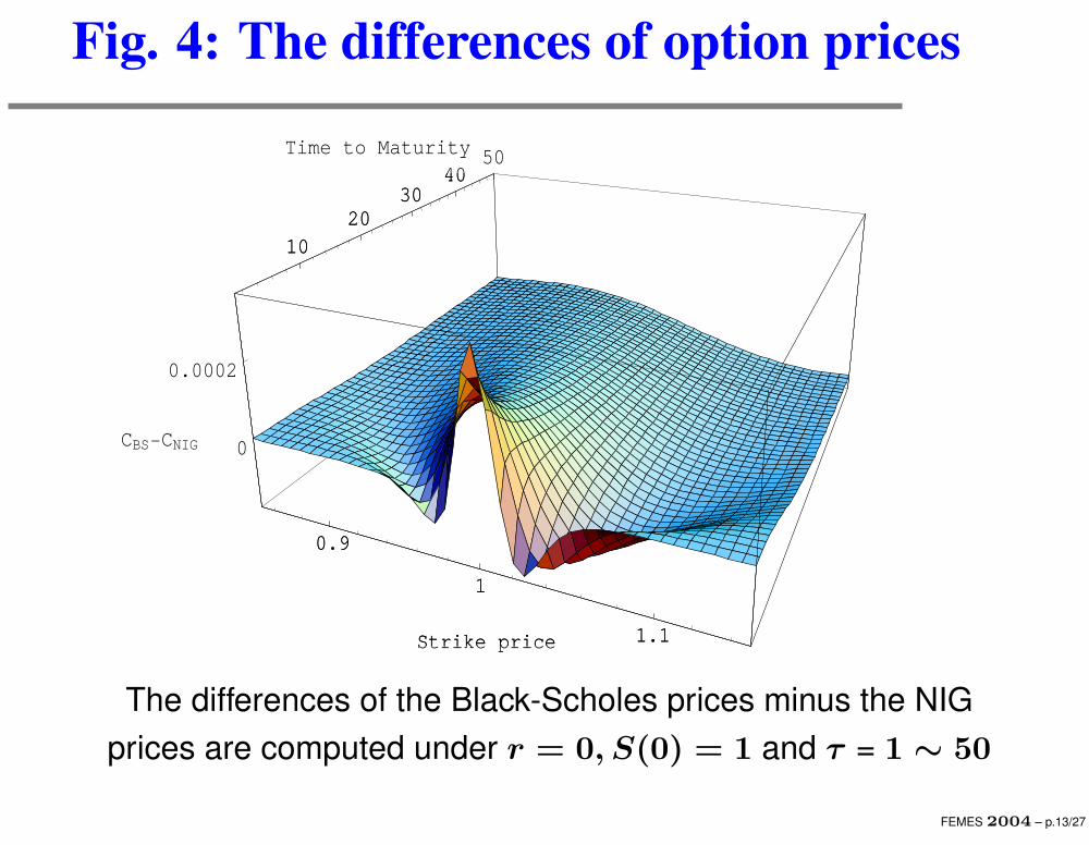
Fig. 4: The differences of option prices

0.9

1

1.1Strike price

1020

3040

50Time to Maturity

0

0.0002

CBS-CNIG

0.9

1

1.1Strike price

1020

3040

The differences of the Black-Scholes prices minus the NIG

prices are computed under r = 0, S(0) = 1 and τ = 1 ∼ 50

FEMES 2004 – p.13/27

The empirical study — About data set

As the Japanese market data, we use

the closing prices of the Nikkei 225 call option fromSeptember 10, 1999 to December 12, 2002.

the Nikkei 225 Stock Average index

We exclude call options

with trading volume less than 10 units

with greater than 100 days to expiration

FEMES 2004 – p.14/27

The empirical study — parameters estimation

● The Black-Scholes model： Historical volatility σ

We estimate the historical volatility from returns of 20

days before the option trading day.

● The NIG model：α, β, δ, µ

We estimate the parameters from returns of 1000 days

before the option trading day.

FEMES 2004 – p.15/27

The criterion to compare the pricing performance

To compare the performances of option pricing models,we compute the pricing errors between observed marketprices and model prices by

1. Mean absolute error rate(MAER)

1

M

M∑

i=1

∣

∣

∣

∣

∣

Ci − Ci

Ci

∣

∣

∣

∣

∣

(5)

2. Weighted mean absolute error rate

M∑

i=1

∣

∣

∣

∣

∣

Ci − Ci

Ci

∣

∣

∣

∣

∣

wi, wi =Vi

M∑

i=1

Vi

(6)

Ci · · · model price，Ci · · · market price，Vi · · · trading volume

FEMES 2004 – p.16/27

Table 2: MAER and Weighted MAER

Table 2: The pricing errors for BS and NIG models

BS model NIG model sample size

MAER 0.4625 0.3242 16063

Weighted MAER 0.5108 0.4084 16063

Next, we plot the pricing errors which are calculatedfrom each classified option data according to theterm to expiration.

FEMES 2004 – p.17/27

Fig. 5: The pricing errors at each term to expiration

MAER Weighted MAER

1 25 50 75 1000

0.1

0.2

0.3

0.4

0.5

0.6

0.7

0.8

Time to maturity

MAER

BSNIG

1 25 50 75 1000

0.1

0.2

0.3

0.4

0.5

0.6

0.7

0.8

0.9

1

Time to maturity

Weighted MAER

BSNIG

The pricing errors on each classification data by the samelength of time to expiration

FEMES 2004 – p.18/27

The classification by moneyness (S(0)/K)

To look at the pricing performance from a different aspect

we classify option data into the following five categories by

the size of moneyness S(0)/K:

1 : S(0)/K < 0.91, Deep-out-of-the-money (DOTM)

2 : 0.91 ≤ S(0)/K < 0.97, Out-of-the-money (OTM)

3 : 0.97 ≤ S(0)/K < 1.03, At-the-money (ATM)

4 : 1.03 ≤ S(0)/K < 1.09, In-the-money (ITM)

5 : 1.09 ≤ S(0)/K, Deep-in-the-money (DITM)

We use the size of the ratio according to Watanabe(2003).

FEMES 2004 – p.19/27

Table 3: MAER in each category

Table 3: MAER

Moneyness BS model NIG model Sample size

DOTM 0.8243 0.5194 6203

OTM 0.3929 0.3337 3996

ATM 0.1836 0.1583 3220

ITM 0.0761 0.0675 1467

DITM 0.0390 0.0371 1177

FEMES 2004 – p.20/27

Table 4: Weighted MAER in each category

Table 4: Weighted MAER

Moneyness BS model NIG model Sample size

DOTM 0.7947 0.5998 6203

OTM 0.4701 0.3871 3996

ATM 0.2444 0.2232 3220

ITM 0.0692 0.0681 1467

DITM 0.0409 0.0400 1177

FEMES 2004 – p.21/27

Fig. 6: Pricing errors (DOTM)

MAER Weighted MAER

1 25 50 75 1000

0.5

1

1.5

Time to maturity

MAER

BSNIG

1 25 50 75 1000

0.5

1

1.5

Time to maturity

Weighted MAER

BSNIG

FEMES 2004 – p.22/27

Fig. 7: Pricing errors (OTM)

MAER Weighted MAER

1 25 50 75 1000

0.2

0.4

0.6

0.8

1

Time to maturity

MAER

BSNIG

1 25 50 75 1000

0.2

0.4

0.6

0.8

1

Time to maturity

Weighted MAER

BSNIG

FEMES 2004 – p.23/27

Fig. 8: Pricing errors (ATM)

MAER Weighted MAER

1 25 50 74 1000

0.05

0.1

0.15

0.2

0.25

0.3

0.35

0.4

Time to maturity

MAER

BSNIG

1 25 50 74 1000

0.1

0.2

0.3

0.4

0.5

Time to maturity

Weighted MAER

BSNIG

FEMES 2004 – p.24/27

Fig. 9: Pricing errors (ITM)

MAER Weighted MAER

1 23 46 69 1000

0.05

0.1

0.15

0.2

0.25

Time to maturity

MAER

BSNIG

1 23 46 69 1000

0.05

0.1

0.15

0.2

0.25

Time to maturity

Weighted MAER

BSNIG

FEMES 2004 – p.25/27

Fig. 10: Pricing errors (DITM)

MAER Weighted MAER

1 24 47 70 1000

0.02

0.04

0.06

0.08

0.1

0.12

0.14

Time to maturity

MAER

BSNIG

1 24 47 70 1000

0.02

0.04

0.06

0.08

0.1

0.12

0.14

Time to maturity

Weighted MAER

BSNIG

FEMES 2004 – p.26/27

Summary

From the empirical evidence on Japanese market,the NIG distribution provides a better fit to the returnsof the Nikkei 225 than the Normal distribution.

⇓

It is appropriate that we use the NIG distribution todescribe the features of assets returns.

As suggested by the results of pricing errors, the NIGmodel can capture the behavior of the market datamore accurately than the Black-Scholes model.

FEMES 2004 – p.27/27