or lectures 2011 - part 1
DESCRIPTION
1-What's operation Researches2-The evolution of managment thinking3-Histroy of ORTRANSCRIPT

1
Prof. M. Hamdy E lwany
1 s t Ye a r P ro d u c ti o n E n g i n e e r i n g D e p a r t m e nt2 0 1 1
Operations Research

2
Lecture 1
What is Operations Research?

3
The Evolution of Management Thinking

4
Management Perspectives Over Time
1930
Humanistic Perspective19901890
Classical1940
1950
2000Systems Theory
2000
2010The Technology-Driven Workplace
1990
2010The Learning Organization
1970
Contingency Views2000
1980
Total Quality Management2000
1940
Management Science Perspective1990
20101870

5
Forces Influencing Organizations and Management
Social Forces - values, needs, and standards of behavior
Political Forces - influence of political and legal institutions on people & organizations
Economic Forces - forces that affect the availability, production, & distribution of a society’s resources among competing users

6
Classical Perspective: 3000 B.C.
Rational, scientific approach to management make organizations efficient operating machines
Scientific Management
Bureaucratic Organizations
Administrative Principles

7
Scientific Management: Taylor 1856-1915
Developed standard method for performing each job.
Selected workers with appropriate abilities for each job.
Trained workers in standard method.Supported workers by planning work and
eliminating interruptions.Provided wage incentives to workers for
increased output.

8
Scientific Management
Contributions Demonstrated the importance of compensation for
performance. Initiated the careful study of tasks and jobs. Demonstrated the importance of personnel and their
training.Criticisms
Did not appreciate social context of work and higher needs of workers.
Did not acknowledge variance among individuals. Tended to regard workers as uninformed and ignored
their ideas

9
Humanistic Perspective
Emphasized understanding human behavior, needs, and attitudes in the workplace
Human Relations Movement
Human Resources Perspective
Behavioral Sciences Approach

10
Management Science Perspective
Emerged after World War II.Applied mathematics, statistics, and other
quantitative techniques to managerial problems Operations Research – mathematical modeling Operations Management – specializes in physical
production of goods or services Information Technology – reflected in management
information systems

11
Recent Historical Trends
Systems Theory
Contingency View
Total Quality Managemen
t (TQM)

12
An Introduction to Operations Research

13
What is Operations Research?
Operations Research (OR) seeks the determination of the best (optimum) course of action of a decision problem under the restriction of limited resources.
The term operations research quite often is associated with the use of mathematical techniques to model and analyze decision problems.

14
History of OR
The beginning of the activity called Operations Research has generally been attributed to the military services early in the World War II.
There was an urgent need to allocate scarce resources to the various military operations and to the activities within each operation in an effective manner.
Therefore, the British and then the US military management called upon a large number of scientists.

15
History of OR Cont.
The scientists were asked to do research in Military Operations. These teams of scientists were, thus, the first Operations Research teams.
Through their research on how to better manage convoy and antisubmarine operations, they also played a major role in winning of: Air battle of Britain The battle of the North Atlantic. Island Campaign in the Pacific.

16
History of OR Cont.
After the success of OR in military operations, increase attention in the use of OR in industrial and organizational applications.
By the early 1950s, OR was used in a variety of organizations in business, industry, and government.
The rapid spread of OR soon followed.

17
History of OR Cont.
Two important factors played an important role in rapid growth of OR The substantial progress that was made early in
improving the techniques to OR Simplex method for solving linear programming problems,
developed by George Dantzig in 1947 Many of the standard tools of OR, such as linear
programming, dynamic programming, queuing theory, and inventory theory, were relatively well developed before the end of the 1950s.
Computer revolution The development of personal computers.

18
OR as A Problem Solving Technique
OR must be viewed as both: A science
Providing mathematical techniques and algorithms for solving appropriate decision problems.
An art as success in all the phases that precede and succeed the
solution of a mathematical model depends largely on the creativity and personal abilities of the decision-making analyst.

19
OR as A Problem Solving Technique
There are three main phases to use OR approach: Phase I: PROBLEM ANALYSIS
Define the Operations Research Analyze the problem and divide into smaller units Establish research priorities
Phase II: SOLUTION DEVELOPMENT Specify solution objectives Specify decision variables and stipulate constraints on the solution Identify or construct an appropriate model for solution
development Determine and obtain required data Develop solutions using analytical mode
20
OR as A Problem Solving Technique
Phase III: SOLUTION VALIDATION Design field test Implement field test Evaluate the propose solution Modify if necessary Integrate the solution with the larger system
Thus implementing OR approach depends on the ability of the OR team to establish good lines of
communication with the sources of information as well as with the individuals responsible for implementing recommended solutions.

21
Lecture 2
An Introduction to Linear Programming

22
Linear Programming (LP)
Linear Programming has proven to be one of the most effective operations research tools.
LP success stems from its flexibility in describing multitudes of real-life situations in the following areas: military, industry, agriculture, transportation, behavioral and
social sciences, economic sciences, … etc. LP is a mathematical modeling technique used to
determine a level of operational activity in order to achieve an objective, subject to restrictions called constraints

23
Model Formulation
Model Formulation: The first step in solving an LP model is building the mathematical model according to the following steps:
1. Determine decision variables: What does the model seek to determine? (mathematical symbols representing levels of activity of an operation)
2. Determine the objective function: A linear relationship reflecting the objective of an operation
Most frequent objective of business firms is to maximize profit Most frequent objective of individual operational units (such as a
production or packaging department) is to minimize cost
3. Determine the constraints: What restrictions must be imposed on the variables to satisfy the limitations of the modeled system? (represented by linear relationship)

24
Model Formulation
The general form of LP mathematical model will be as follows:
Max/min z = c1x1 + c2x2 + ... + cnxn
subject to:a11x1 + a12x2 + ... + a1nxn (≤, =, ≥) b1a21x1 + a22x2 + ... + a2nxn (≤, =, ≥) b2
:am1x1 + am2x2 + ... + amnxn (≤, =, ≥) bm
xj = decision variablesbi = constraint levelscj = objective function coefficientsaij = constraint coefficients

25
LP Model: Example 1
Labor Clay RevenuePRODUCT (hr/unit) (lb/unit) ($/unit)Bowl 1 4 40Mug 2 3 50
RESOURCE REQUIREMENTS
There are 40 hours of labor and 120 pounds of clay available each dayStep 1: Decision variables
x1 = number of bowls to produce
x2 = number of mugs to produce

26
LP Model: Example 1
Labor Clay RevenuePRODUCT (hr/unit) (lb/unit) ($/unit)Bowl 1 4 40Mug 2 3 50
RESOURCE REQUIREMENTS
There are 40 hours of labor and 120 pounds of clay available each dayStep 2: Objective Function
Maximize Z = $40 x1 + 50 x2
– Maximize Profit

27
LP Model: Example 1
Labor Clay RevenuePRODUCT (hr/unit) (lb/unit) ($/unit)Bowl 1 4 40Mug 2 3 50
RESOURCE REQUIREMENTS
There are 40 hours of labor and 120 pounds of clay available each dayStep 3: Constraints
x1+ 2x2 < 40 hr (labor constraint)4x1+ 3x2 < 120 lb (clay constraint)x1 , x2 > 0 (Non-negativity constraint)
Subject to:

28
LP Model: Example 1
We can write the mathematical model as one block as follows:
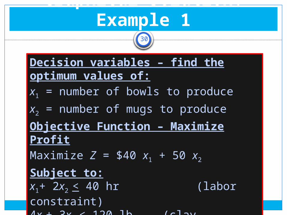
Decision variables – find the optimum values of:x1 = number of bowls to produce
x2 = number of mugs to produce
Objective Function – Maximize ProfitMaximize Z = $40 x1 + 50 x2
Subject to:x1+ 2x2 < 40 hr (labor constraint)4x1+ 3x2 < 120 lb (clay constraint)x1 , x2 > 0 (Non-negativity constraint)

29
Solving LP Problems
Graphical Solution method: is one of the most common tools in solving LP models
The steps of solving the LP problems using the graphical solution method:1. Plot model constraint on a set of coordinates in a plane.2. Identify the feasible solution space on the graph where
all constraints are satisfied simultaneously.3. Plot objective function to find the point on boundary of
this space that maximizes (or minimizes) value of objective function.
30
Graphical Solution: Example 1
Decision variables – find the optimum values of:x1 = number of bowls to produce
x2 = number of mugs to produce
Objective Function – Maximize ProfitMaximize Z = $40 x1 + 50 x2
Subject to:x1+ 2x2 < 40 hr (labor constraint)4x1+ 3x2 < 120 lb (clay constraint)x1 , x2 > 0 (Non-negativity constraint)

31
Graphical Solution: Example 1
4 x1 + 3 x2 <120 lb
x1 + 2 x2 <40 hr
Area common toboth constraints(Feasibility Region)
50 –
40 –
30 –
20 –
10 –
0 –|
10|
60|
50|
20|
30|
40 x1
x2
Maximize Z = $40 x1 + 50 x2
Optimal point:
x1 = 24 bowls,
x2 =8 mugs
Z = $1360

32
Graphical Solution: Example 2
Find the maximum and minimum values of the function z =3x1 + 5x2, given the following set of constraints,3 x1 + 2 x2 < 18
x1 < 4
2 x2 < 12
x1 and x2 > 0

33
Graphical Solution: Example 2
To solve this problem, follow the following steps:1. Represent the given inequalities and find the
solution space.2. Represent the given function, and find its direction
of increase and decrease.3. Find the points that would both belong to the
solution space and give the maximum and minimum values of the function.

34
Graphical Solution: Example 2
Representing the Inequalities

35
Graphical Solution: Example 2
Draw the objective function equation
with (0,0)

36
Graphical Solution: Example 2
The direction of decrease is the one downwards and
vice versa.
Increase
Decrease

37
Graphical Solution: Example 2
shift the straight line in the direction of increase till it reaches the furthest
point that still belongs to solution space

38
Graphical Solution: Example 2
shift the straight line in the direction of increase till it reaches the furthest
point that still belongs to solution space

39
Graphical Solution: Example 2
The Optimum Solution at (2,6) Therefore the objective function = 36
X1 = 2X2 = 6Z = 36

40
Example 3: Model Formulation
Shirtstop makes t-shirts with logos and sells them in its chain of retail stores.
They contract with two different plants—one in Puerto Rico and one in the Bahamas.
The shirts from the plant in Puerto Rice cost $0.46 apiece and 9% of them are defective and can't be sold.
The shirts from the Bahamas cost only $0.35 each but they have an 18% defective rate. Shirtstop needs 3,500 shirts.
To retain their relationship with the two plants they want to order at least 1,000 shirts from each.
They would also like at least 88% of the shirts they receive to be salable.
Formulate a linear programming model for this problem.

41
Example 3: Model Formulation
Decision variables – find the optimum values of:X1: Number of t-shirts bought from the plant in Puerto Rico
X2: Number of t-shirts bought from the plant in Bahamas
Objective Function – Minimize CostMinimize Z = 0.46X1 + 0.35X2
Subject to:X1 > 1000, X2 > 10000.82X1 + 0.91X2 > 35000.82X1 + 0.91X2 > 0.88 (X1 + X2)X1, X2 > 0

42
Lecture 2 – (Cont ’d)Examples
An Introduction to Linear Programming

Example 143
Find the maximum values of the function z = 5x + 2y, given the following set of constraints: 2x + 3y ≥ 6, 3x + 2y ≥ 6, x and y ≥ 0

Solution44
3 –
2 –
1 -
1 2 3 I I I
2x + 3y ≥ 6
3x + 2y ≥ 6
(Unbounded Solution)

Example 2 (Infeasible Solution)45
Find the minimum values of the function z = 5x + 2y, given the following set of constraints: 3x + 3y ≤ 9, 4x + 5y ≥ 20, x and y ≥ 0

Solution46
5 –
4 -
3 -
2 –
1 -
1 2 3 4 5 I I I I I
4x + 5y ≥ 20
3x + 3y ≤ 9
(Infeasible Solution)

Example 3 (Redundant Constraint)47
Find the maximum values of the function z = 3x1 + 5x2, given the following set of constraints: x1 ≤ 4, 2x2 ≤ 12, 3x1 + 2x2 ≤ 18, 3x1 + 5x2 ≤ 50, x1 and x2 ≥ 0

Solution48
13 -12 -11 -10 – 9 - 8 - 7- 6 - 5 - 4 - 3 – 2 – 1 -
1 2 3 4 5 6 7 8 9 10 11 12 13 14 15 16 17 I I I I I I I I I I I I I I I I I
Optimum Solution
Z= 36X1 =2X2 = 6
Redundant Constraint
4x + 5y ≥ 20
4x + 5y ≥ 20
4x + 5y ≥ 20
4x + 5y ≥ 20

Solution (Change Objective)49
13 -12 -11 -10 – 9 - 8 - 7- 6 - 5 - 4 - 3 – 2 – 1 -
1 2 3 4 5 6 7 8 9 10 11 12 13 14 15 16 17 I I I I I I I I I I I I I I I I I
Optimum Solution
Z= 18X1 =4X2 = 3
If z = 3x1 + 2x2

Example 450
Find the minimum value of the given functionz = 3 x1 – 2 x2, and the point at which it occurs, for the given set of constraints: 4 x1 + 5 x2 < 20 x1 + x2 > 3 x1 = 1 x1 and x2 > 0

Solution51
5 –
4 -
3 -
2 –
1 -
1 2 3 4 5 I I I I I
4 x1 + 5 x2 < 20
x1 = 1
x1 + x2 > 3
z = 3 x1 – 2 x2

Example 5 52
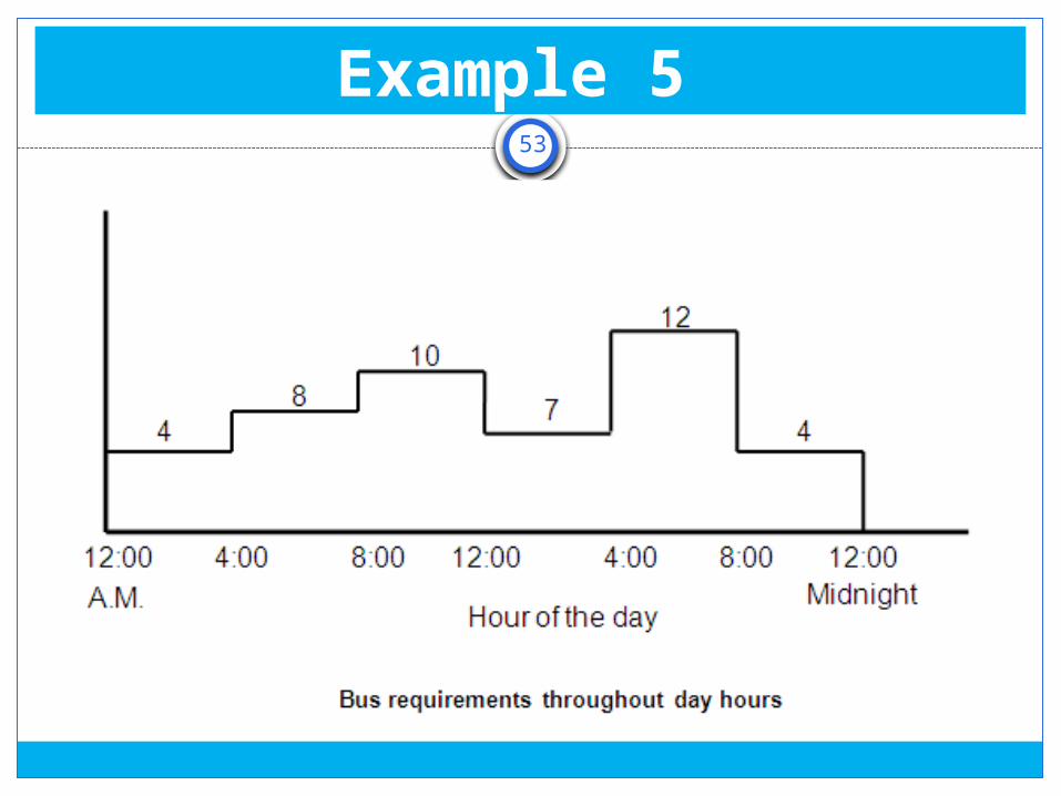
Progress city is studying the feasibility of introducing a mass transit bus system that will reduce the pollution problem by reducing in-city driving. The initial study seeks the determination of the minimum number of buses that can handle transportation needs. After gathering necessary information, the city engineer noticed that the minimum number of buses needed to meet fluctuates with the time of the day. The figure below summarizes the engineer’s findings. It was decided that to carry out the required daily maintenance, each bus could operate only 8 successive hours a day.
Example 5 53

Solution54

Solution55
Decision variables:X1: Number of buses starting at 12:01 A.M.X2: Number of buses starting at 04:01 A.M.X3: Number of buses starting at 08:01 A.M.X4: Number of buses starting at 12:01 P.M.X5: Number of buses starting at 04:01 P.M.X6: Number of buses starting at 08:01 P.M.

Solution56
Objective function:Minimize z = X1 + X2 + X3 + X4 + X5 + X6 Subject to:X1 + X6 > 4X1 + X2 > 8 X2 + X3 > 10 X3 + X4 > 7 X4 + X5 > 12 X5 + X6 > 4X1, X2, X3, X4, X5, X6 > 0

Example 657
A cargo plane has three compartments for storing cargo: front, center, and back. These compartments have capacity limits on both weight and space, as summarized below:
CompartmentWeight capacity
(tons)Space capacity
(cube feet)
Front 12 7000
Center 18 9000
Back 10 5000

Example 658
Furthermore, the weight of the cargo in the respective compartments must be the same proportion of that compartment’s weight capacity to maintain the balance of the airplane. The following four cargoes have been offered for shipment on an upcoming flight as space is available:
Cargo Weight (tons)Volume (cubic
feet/ton)Profit ($/ton)
1 20 500 320
2 16 700 400
3 25 600 360
4 13 400 290

Example 659
Any portion of these cargoes can be accepted. The objective is to determine how much (if any) of each cargo should be accepted and how to distribute each among the compartments to maximize the total profit for the flight. Formulate a linear programming model for this problem.

Solution60
Decision variables: : Number of tons of cargo type 1 stored in the front compartment : Number of tons of cargo type 1 stored in the center compartment : Number of tons of cargo type 1 stored in the back compartment : Number of tons of cargo type 2 stored in the front compartment : Number of tons of cargo type 2 stored in the center compartment : Number of tons of cargo type 2 stored in the back compartment : Number of tons of cargo type 3 stored in the front compartment : Number of tons of cargo type 3 stored in the center compartment : Number of tons of cargo type 3 stored in the back compartment : Number of tons of cargo type 4 stored in the front compartment : Number of tons of cargo type 4 stored in the center compartment : Number of tons of cargo type 4 stored in the back compartment

Solution61
Objective function:Maximize

Solution62
Subject to:

Solution63
Subject to:

Example 764
The pacific paper company produces paper rolls with a standard width of 20 feet each. Special customer orders with different widths are produced by slitting the standard rolls. Typical orders (which may vary from day to day) are summarized in the following table:
Order Desired width (ft)Desired number
of rolls
1 5 150
2 7 200
3 9 300

Example 765
In practice, an order is filled by setting the slitting knives to the desired widths. Usually, there are a number of ways in which a standard roll can be slit to fill a given order. The next figure shows three possible knife settings for the 20-foot roll. Although there are other feasible settings, we limit the discussion for the moment to considering settings A, B, and C. We can combine the given settings in a number of ways to fill orders for widths 5, 7, and 9 feet.

Example 766

Example 767
Find the optimum combination of settings to fulfill the orders while minimizing the trim loss.The following are two feasible combinations:1. Slit 300 (standard rolls) using setting A, and 75 rolls using
setting B.2. Slit 200 rolls using setting A, and 100 rolls using setting C.

Solution68
Required width (ft)
Knife settingsMinimum number of
rolls12
3 4 5 6
5 0 2 2 4 1 0 150
7 11
0 0 2 0 200
9 1 0 1 0 0 2 300
Trim loss per foot of length
4 3 1 0 1 2

Solution69
Decision VariablesXi = Number of standard rolls to be slit according to setting i for I = 1,2, …,6

Solution70
Objective FunctionMinimize Z = X1 + X2 + X3 + X4 + X5 + X6
Subject to2X1 + 2X3 + 4X4 + X5 > 150
X1 + X2 + 2X5 > 200
X1 + X3 + 2X6 > 300
X1, X2, X3, X4, X5, X6 > 0

71
Lecture 3
Solving LP Problems The Simplex Method

72
Introduction
solving LP models using graphical method is only limited to solving models with a maximum number of two decision variables.
When the number of variables exceeds this, which is the case in most practical cases, the graphical method becomes inconvenient.
We, thus, seek another method for solving LP models with more than two variables. The most common method is the analytical Simplex method.
The Simplex method is an algorithm (a sequence of steps) that solves LP models. There are many common Simplex algorithms: the extended tableau, the condensed tableau, and the 2-phase method.

73
LP Terminologies
Feasible solution: The set of feasible solutions to a linear programming problem form a convex set for which all included points satisfy all constraints and non-negativity conditions.
Infeasible solution: Any point that does not satisfy all the constraints and non-negativity conditions is termed infeasible.
Basic solution: A basic solution may be identified as the intersection of two (or more) constraints.
Extreme points: The extreme points of the convex set of feasible solutions are equivalent to the set of basic feasible solutions.
Optimal solution: The optimal solution to a given linear programming problem, if it exists, will occur at one or more extreme points.

74
Steps of the Simplex Process
The general steps to the Simplex process are:1. Begin the search at an extreme point (a basic feasible
solution).
2. Determine if movement to an adjacent extreme point can improve on the optimization of the objective function. If not, then present solution is optimal.
3. Move to the adjacent extreme point which offers the most improvement in the objective function.
4. Continue steps 2 and 3 until the optimal solution is found or until it can be shown that the problem is either unbounded or infeasible.

75
Standard LP Form
The properties of this form are as follows: All the constraints are equations. All the variables are nonnegative. The objective function may be maximization or
minimization
We shall call the inequalities with the sign of “<” Type I inequalities and inequalities of the sign “>” Type II inequalities.

76
Standard LP Form
Type I inequalities “<” In the constraint X1 + 2X2 < 6,
Converting it to this equation X1 + 2X2 + S1 = 6 (Adding a Slack Variable)
Type II inequalities “>” In the constraint 3X1 + 2X2 – 3X3 ≥ 5
Converting it to this equation 3X1 + 2X2 – 3X3 – S2 = 5 (Adding a Surplus Variable)

77
Standard LP Form
The Artificial Variable is added to overcome the negative value of the Surplus variable, the artificial variable doesn’t have any physical significance; it is truly an artificial device employed to drive an immediate recognizable basic feasible solution.
Example: 3X1 + 2X2 – 3X3 ≥ 5
Converting it to this equation 3X1 + 2X2 – 3X3 – S2 + R1 = 5

78
Standard LP Form
Impact on the objective function For Simplicity, the objective functions should be
considered as the maximization form. Thus, when dealing with a minimization objective, we
simply multiply the objective by –1 and maximize it.
Given a maximization objective z, r surplus variables, and t artificial variables, the modified objective is:
n
j
r
k
t
pppkkjj Rcscxcz
1 1 1
Maximize

79
Standard LP Form
n
j
r
k
t
pppkkjj Rcscxcz
1 1 1
Maximize
Original Objective Function
Impact of the slack and surplus variablesWhere ck = zero
Impact of the artificial variablesWhere cp = -M

80
Example on an LP Model
Maximize Z = 7X1 – 3X2 + 5X3
Subject to,
X1 + X2 + X3 > 9
3X1 + 2X2 + X3 < 12
X1, X2, X3 > 0

81
Transforming it to the Standard LP Form
The new ConstraintsX1 + X2 + X3 - S1 + R1 = 9
3X1 + 2X2 + X3 + S2 = 12
X1, X2, X3, S1, S2, and R1 > 0The new Objective Function
Maximize z= 7X1 – 3X2 + 5X3 + 0S1 – MR1 + 0S2
Note: we will use (X) instead of S and R

82
Transforming it to the Standard LP Form
The new ConstraintsX1 + X2 + X3 -X4 + X5 = 9
3X1 + 2X2 + X3 + X6 = 12
X1, X2, X3, X4, X5, and X6 > 0The new Objective Function
Maximize z= 7X1 – 3X2 + 5X3 + 0X4 – MX5 + 0X6
Therefore the solution will become

83
The Extended Tableau
After transforming the problem to the standard LP form, we set up the initial extended tableau as follows:Coefficient
of the Basic
Variables
Basic Variables
Labels
Variable Labels Basic Feasible Solution Values
X1 X2 … Xn
CB, 1 XB, 1 y1,1 y1,2 … y1,n XB,1
. . . . . . .
. . . . . . .
. . . . . . .CB, m XB, m ym,1 ym,2 … ym,n XB,m
Indicator Row z1 – c1 z2 – c2 … zn – cn z

84
The Extended Tableau
After transforming the problem to the standard LP form, we set up the initial extended tableau as follows:
Where,CB,m: The coefficient of the basic variable number “m” in
the objective function.XB,m: The basic variable number “m”ym,n: The coefficient of the variable number “n” in the constraint associated with basic variable number “m”zn – cn: The indicator value of variable number “n”. You’ll learn how to calculate it.

85
Example
Given the following problem, setup the initial extended tableau, then find the optimum solution to the problem using the Simplex algorithm.
Maximize z = 6X1 + 8X2
Subject to,4X1 + X2 ≤ 20
X1 + 4X2 ≤ 40
X1, X2 ≥ 0

86
Step 1: Find Standard LP Form
Maximize z = 6X1 + 8X2 + 0X3 + 0X4
Subject to,4X1 + X2 + X3 = 20
X1 + 4X2 + X4 = 40
X1, X2, X3, X4 ≥ 0

87
Step 2: Construct the Initial Extended Tableau
cj 6 8 0 0
cB BV X1 X2 X3 X4 XB
0 X3
0 X4

88
Step 2: Construct the Initial Extended Tableau
Fill in the values of yi,j
cj 6 8 0 0
cB BV X1 X2 X3 X4 XB
0 X3 4 1 1 0
0 X4 1 4 0 1

89
Step 2: Construct the Initial Extended Tableau
Fill in the values of the starting basic feasible solution
cj 6 8 0 0
cB BV X1 X2 X3 X4 XB
0 X3 4 1 1 0 20
0 X4 1 4 0 1 40

90
Step 2: Construct the Initial Extended Tableau
Calculate the indicator row, as follows:zj – cj = cbyj – cj
cj 6 8 0 0
cB BV X1 X2 X3 X4 XB
0 X3 4 1 1 0 20
0 X4 1 4 0 1 40

91
Step 2: Construct the Initial Extended Tableau
Calculate the indicator row, as follows:z1 – c1 = [(4x0) + (1x0)] – 6 = -6
cj 6 8 0 0
cB BV X1 X2 X3 X4 XB
0 X3 4 1 1 0 20
0 X4 1 4 0 1 40
-6
92
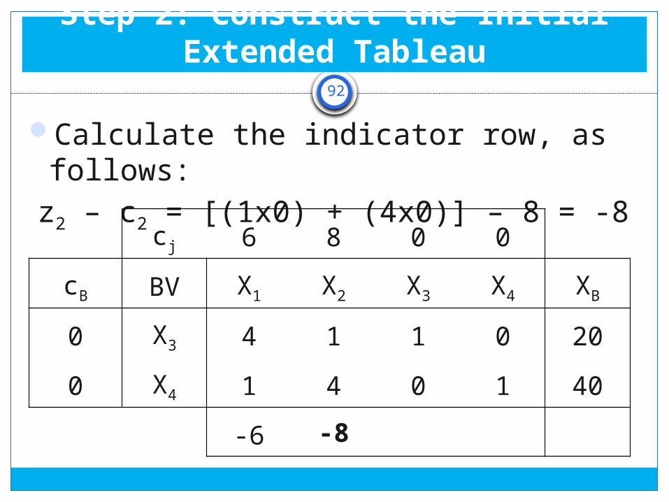
Step 2: Construct the Initial Extended Tableau
Calculate the indicator row, as follows:z2 – c2 = [(1x0) + (4x0)] – 8 = -8
cj 6 8 0 0
cB BV X1 X2 X3 X4 XB
0 X3 4 1 1 0 20
0 X4 1 4 0 1 40
-6 -8

93
Step 2: Construct the Initial Extended Tableau
Therefore the indicator row is as follows:
cj 6 8 0 0
cB BV X1 X2 X3 X4 XB
0 X3 4 1 1 0 20
0 X4 1 4 0 1 40
-6 -8 0 0
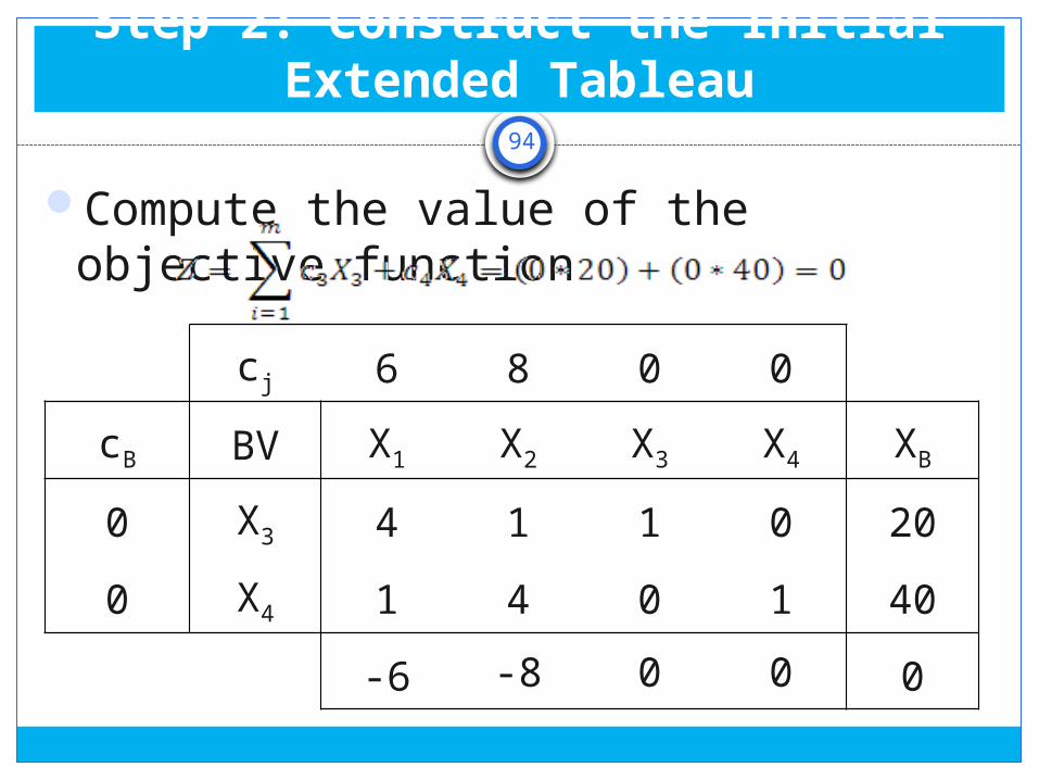
94
Step 2: Construct the Initial Extended Tableau
Compute the value of the objective function
cj 6 8 0 0
cB BV X1 X2 X3 X4 XB
0 X3 4 1 1 0 20
0 X4 1 4 0 1 40
-6 -8 0 0 0

95
Step 2: Construct the Initial Extended Tableau
This is one of the feasible solutions (iteration 0). If there are negative values in the indicator row, you can reach a better solution by continuing with the following steps.
cj 6 8 0 0
cB BV X1 X2 X3 X4 XB
0 X3 4 1 1 0 20
0 X4 1 4 0 1 40
-6 -8 0 0 0

96
cj 6 8 0 0
cB BV X1 X2 X3 X4 XB
0 X3 4 1 1 0 20
0 X4 1 4 0 1 40
-6 -8 0 0 0
Step 3: Determine the Entering Variable
The variable having the most negative zj – cj value. The entering variable is X2 (because its zj – cj is equal to -8).

97
cj 6 8 0 0
cB BV X1 X2 X3 X4 XB
0 X3 4 1 1 0 20
0 X4 1 4 0 1 40
-6 -8 0 0 0
Step 4: Determine the Departing Variable
Divide the XB column by the yi column of the entering variable, and choosing the least nonnegative value as the departing (leaving) variable.

98
cj 6 8 0 0
cB BV X1 X2 X3 X4 XB
0 X3 4 1 1 0 20
0 X4 1 4 0 1 40
-6 -8 0 0 0
Step 4: Determine the Departing Variable

99
cj 6 8 0 0
cB BV X1 X2 X3 X4 XB
0 X3 4 1 1 0 20
0 X4 1 4 0 1 40
-6 -8 0 0 0
Step 4: Determine the Departing Variable
Pivot Element (yij)

100
Step 5: Construct the new tableau “iteration 1”
Replace the departing variable with the entering variable.
cj 6 8 0 0
cB BV X1 X2 X3 X4 XB
0 X3
8 X2

101
Step 5: Construct the new tableau “iteration 1”
The row of the entering variable in the new tableau (i.e. row number i) is obtained by dividing the old row i’ by the pivot element.
cj 6 8 0 0
cB BV X1 X2 X3 X4 XB
0 X3
8 X2 1/4 1 0 1/4 10

102
Step 5: Construct the new tableau “iteration 1”
The column of the departing variable in the new tableau is all equal to zero, except to the element in the entering variable row which is equal to one.
cj 6 8 0 0
cB BV X1 X2 X3 X4 XB
0 X3 0
8 X2 1/4 1 0 1/4 10
0

103
Step 5: Construct the new tableau “iteration 1”
The remaining elements of the tableau are calculated using the following relations.
cj 6 8 0 0
cB BV X1 X2 X3 X4 XB
0 X3 0
8 X2 1/4 1 0 1/4 10
0

104
Step 5: Construct the new tableau “iteration 1”
The remaining elements of the tableau are calculated using the following relations.
cj 6 8 0 0
cB BV X1 X2 X3 X4 XB
0 X3 0
8 X2 1/4 1 0 1/4 10
0

105
Step 5: Construct the new tableau “iteration 1”
The remaining elements of the tableau are calculated using the following relations.
cj 6 8 0 0
cB BV X1 X2 X3 X4 XB
0 X3 15/4 0
8 X2 1/4 1 0 1/4 10
0

106
Step 5: Construct the new tableau “iteration 1”
The remaining elements of the tableau are calculated using the following relations.
cj 6 8 0 0
cB BV X1 X2 X3 X4 XB
0 X3 15/4 0 -1/4
8 X2 1/4 1 0 1/4 10
0

107
Step 5: Construct the new tableau “iteration 1”
The remaining elements of the tableau are calculated using the following relations.
cj 6 8 0 0
cB BV X1 X2 X3 X4 XB
0 X3 15/4 0 1 -1/4
8 X2 1/4 1 0 1/4 10
0

108
Step 5: Construct the new tableau “iteration 1”
The remaining elements of the tableau are calculated using the following relations.
cj 6 8 0 0
cB BV X1 X2 X3 X4 XB
0 X3 15/4 0 1 -1/4 10
8 X2 1/4 1 0 1/4 10
0

109
Step 5: Construct the new tableau “iteration 1”
The remaining elements of the tableau are calculated using the following relations.
cj 6 8 0 0
cB BV X1 X2 X3 X4 XB
0 X3 15/4 0 1 -1/4 10
8 X2 1/4 1 0 1/4 10
-4 0

110
Step 5: Construct the new tableau “iteration 1”
Calculate the new objective value and indicator row, and the final form of the new tableau is given as follows.
cj 6 8 0 0
cB BV X1 X2 X3 X4 XB
0 X3 15/4 0 1 -1/4 10
8 X2 1/4 1 0 1/4 10
-4 0 0 2 80

111
Repeat Steps 3 and 4 for Iteration 2
The first iteration tableau with the entering and departing variables shown.
cj 6 8 0 0
cB BV X1 X2 X3 X4 XB
0 X3 15/4 0 1 -1/4 10
8 X2 1/4 1 0 1/4 10
-4 0 0 2 80

112
Repeat Steps 5 for Iteration 2
The completed second iteration tableau
cj 6 8 0 0
cB BV X1 X2 X3 X4 XB
6 X1 1 0 4/15 -1/15 8/3
8 X2 0 1 -1/15 4/15 28/3
0 0 16/15 26/15 272/3

113
Repeat Steps 5 for Iteration 2
Now, since all the zj – cj are nonnegative, and there are no artificial variables in the basis, we have reached the optimal solution.
cj 6 8 0 0
cB BV X1 X2 X3 X4 XB
6 X1 1 0 4/15 -1/15 8/3
8 X2 0 1 -1/15 4/15 28/3
0 0 16/15 26/15 272/3

114
The Optimum Solution
X*1 = 8/3X*2 = 28/3X*3 = 0X*4 = 0z* = 272/3

115
Summary
We can summarize the Simplex algorithm in the following steps,1. Find standard LP form2. Find the starting basic solution by constructing the
initial tableau3. Decide whether the solution is now optimal,
infeasible, unbounded, or can be improved according to the following diagram.

116
Summary
Check indicator row (zj - cj)
There are negative values (Do not
stop)
There are positive ratios (Solution can
be further improved)
There are no negative ratios
(Solution is unbounded)
There are no negative values
(Stop)
There are artificial variables in the
basis (Solution is infeasible)
There are no artificial variables
in the basis (Solution is
optimal)

117
Summary
4. If the solution is optimal, infeasible, or unbounded, then the problem is completed. If the solution can be improved, then do a new iteration.
5. Go to step III.

118
Lecture 4
Special Types of LP Problems

119
Special Features
There are a number of particular features that tend to identify or isolate the special problem classes that are presented. 1. Variables: are usually integers and could also be of
binary value.2. Network Representation: consists of:
Nodes Branches
3. Computational Complexity

120
Lecture 4 – A
The Transportation Problem

121
The Transportation Problem
A transportation problem basically deals with the problem, which aims to find the best way to fulfill the demand of n demand points (sources) using the capacities of m supply points (sinks). While trying to find the best way, generally a variable cost of shipping the product from one supply point to a demand point or a similar constraint should be taken into consideration.

122
The Transportation Problem (Cont’d)
BB
CC
AA
IIII
IIIIII
IVIV
Sou
rces
II
`̀
[10]
[15]
[15]
[8]
[12]
[10]
[10]
Sinks
(2)
(2)(2)
(3)
(3)
(4)
(7)
(5) (1)
(7)
(6)
(6)

123
Formulating Transportation Problems
Example 1: Powerco has three electric power plants that supply the electric needs of four cities:• The associated supply of each plant and demand of
each city is given in the table 1.• The cost of sending 1 million kwh of electricity from a
plant to a city depends on the distance the electricity must travel.

124
The Transportation Table
A transportation problem is specified by the supply, the demand, and the shipping costs. So the relevant data can be summarized in a transportation tableau. The transportation table implicitly expresses the supply and demand constraints and the shipping cost between each demand and supply point.

125
The Transportation Table
Table 1. Shipping costs, Supply, and Demand for Powerco Example
From To
City 1
City 2 City 3 City 4
Supply (Million
kwh)
Plant 1 $8 $6 $10 $9 35
Plant 2 $9 $12 $13 $7 50
Plant 3 $14 $9 $16 $5 40Demand
(Million kwh)45 20 30 30

126
Solution
1.Decision Variable: Since we have to determine how much electricity is sent from each plant to each city; Xij = Amount of electricity produced at plant i
and sent to city j X14 = Amount of electricity produced at plant
1 and sent to city 4

127
Solution (Cont’d)
2. Objective Function: Since we want to minimize the total cost of shipping from plants to cities;
Minimize Z = 8X11+6X12+10X13+9X14+9X21+ 12X22+13X23+7X24 +14X31+9X32+16X33+5X34
3. Supply Constraints: Since each supply point has a limited production capacity; X11+X12+X13+X14 <= 35 X21+X22+X23+X24 <= 50 X31+X32+X33+X34 <= 40

128
Solution (Cont’d)
4. Demand Constraints: Since each demand point has a limited production capacity;
X11+X21+X31 >= 45 X12+X22+X32 >= 20 X13+X23+X33 >= 30 X14+X24+X34 >= 30
5.Sign Constraints: Since a negative amount of electricity can not be shipped all Xij’s must be non negative; Xij >= 0 (i= 1,2,3; j= 1,2,3,4)

129
LP Formulation of Powerco’s Problem
Min Z = 8X11+6X12+10X13+9X14+9X21+12X22+13X23
+7X24 +14X31+9X32+16X33+5X34
S.T.: X11+X12+X13+X14 <= 35 (Supply Constraints)X21+X22+X23+X24 <= 50X31+X32+X33+X34 <= 40X11+X21+X31 >= 45 (Demand Constraints)X12+X22+X32 >= 20X13+X23+X33 >= 30X14+X24+X34 >= 30Xij >= 0 (i= 1,2,3; j= 1,2,3,4) (Sign Constraints)

130
General Description of a Transportation Problem
1. A set of m supply points from which a good is shipped. Supply point i can supply at most si units.
2. A set of n demand points to which the good is shipped. Demand point j must receive at least di units of the shipped good.
3. Each unit produced at supply point i and shipped to demand point j incurs a variable cost of cij.

131
General Description of a Transportation Problem
Xij = number of units shipped from supply point i to demand point j
),...,2,1;,...,2,1(0
),...,2,1(
),...,2,1(..
min
1
1
1 1
njmiX
njdX
misXts
Xc
ij
mi
i
jij
nj
j
iij
mi
i
nj
j
ijij

132
Balanced Transportation Problem
If Total supply equals to total demand, the problem is said to be a balanced transportation problem:
nj
j
j
mi
i
i ds11

133
Balancing Transportation Problems
1. Balancing a TP if total supply exceeds total demand:
By adding dummy demand point. Since shipments to the dummy demand point are not real, they are assigned a cost of zero.
2. Balancing a transportation problem if total supply is strictly less than total demand:
There is no doubt that in such a case one or more of the demand will be left unmet. Generally in such situations a penalty cost is often associated with unmet demand and as one can guess this time the total penalty cost is desired to be minimum

134
Finding Basic Feasible Solution for TP
Unlike other Linear Programming problems, a balanced TP with m supply points and n demand points is easier to solve, although it has m + n equality constraints. The reason for that is, if a set of decision variables (xij’s) satisfy all but one constraint, the values for xij’s will satisfy that remaining constraint automatically.
135
Solving a Balanced Transportation Problem
There are three basic Methods to find the basic feasible solution for a balanced Transportation Problem:
1. Northwest Corner Method2. Minimum Cost Method3. Vogel’s Method

136
1. Northwest Corner Method
To find the BFS by the NWC method: Begin in the upper left (northwest) corner of
the transportation tableau and set x11 as large as possible (here the limitations for setting x11 to a larger number, will be the demand of demand point 1 and the supply of supply point 1. Your x11 value can not be greater than minimum of this 2 values).

137
1. Northwest Corner Method (Cont’d)
According to the explanation in the previous slide we can set x11=3 (meaning demand of demand point 1 is satisfied by supply point 1).
5
6
2
3 5 2 3
3 2
6
2
X 5 2 3

138
1. Northwest Corner Method (Cont’d)
After we check the east and south cells, we saw that we can go east (meaning supply point 1 still has capacity to fulfill some demand).
3 2 X
6
2
X 3 2 3
3 2 X
3 3
2
X X 2 3

139
1. Northwest Corner Method (Cont’d)
After applying the same procedure, we saw that we can go south this time (meaning demand point 2 needs more supply by supply point 2).
3 2 X
3 2 1
2
X X X 3
3 2 X
3 2 1 X
2
X X X 2
140
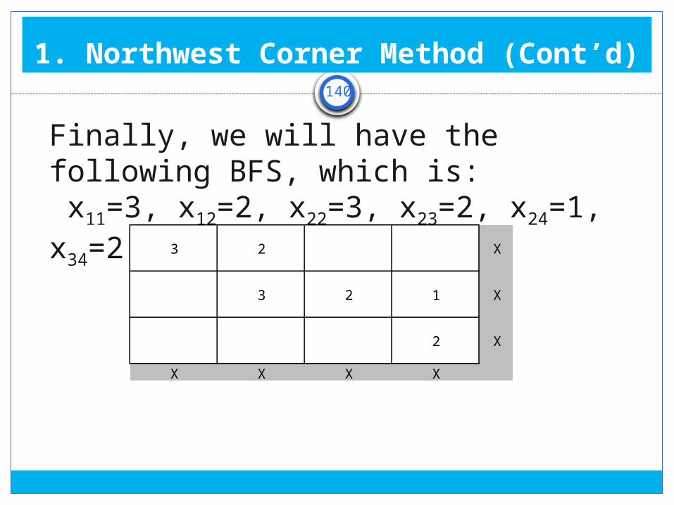
1. Northwest Corner Method (Cont’d)
Finally, we will have the following BFS, which is: x11=3, x12=2, x22=3, x23=2, x24=1, x34=2
3 2 X
3 2 1 X
2 X
X X X X

141
2. Least Cost Method
The Northwest Corner Method dos not utilize shipping costs. It can yield an initial bfs easily but the total shipping cost may be very high.
The least cost method uses shipping costs in order come up with a bfs that has a lower cost.
To begin the least cost method, first we find the decision variable with the smallest shipping cost (Xij). Then assign Xij its largest possible value, which is the minimum of si and dj

142
2. Least Cost Method (Cont’d)
After that, as in the Northwest Corner Method we should cross out row i and column j and reduce the supply or demand of the noncrossed-out row or column by the value of Xij.
Then we will choose the cell with the minimum cost of shipping from the cells that do not lie in a crossed-out row or column and we will repeat the procedure.

143
2. Least Cost Method (Cont’d)
Step 1: Select the cell with minimum cost.
2 3 5 6
2 1 3 5
3 8 4 6
5
10
15
12 8 4 6

144
2. Least Cost Method (Cont’d)
Step 2: Cross-out column 2
2 3 5 6
2 1 3 5
8
3 8 4 6
12 X 4 6
5
2
15

145
2. Least Cost Method (Cont’d)
Step 3: Find the new cell with minimum shipping cost and cross-out row 2
2 3 5 6
2 1 3 5
2 8
3 8 4 6
5
X
15
10 X 4 6

146
2. Least Cost Method (Cont’d)
Step 4: Find the new cell with minimum shipping cost and cross-out row 1
2 3 5 6
5
2 1 3 5
2 8
3 8 4 6
X
X
15
5 X 4 6

147
2. Least Cost Method (Cont’d)
Step 5: Find the new cell with minimum shipping cost and cross-out column 1
2 3 5 6
5
2 1 3 5
2 8
3 8 4 6
5
X
X
10
X X 4 6

148
2. Least Cost Method (Cont’d)
Step 6: Find the new cell with minimum shipping cost and cross-out column 3
2 3 5 6
5
2 1 3 5
2 8
3 8 4 6
5 4
X
X
6
X X X 6

149
2. Least Cost Method (Cont’d)
Step 7: Finally assign 6 to last cell. The BFS is found as: X11=5, X21=2, X22=8, X31=5, X33=4 and X34=6
2 3 5 6
5
2 1 3 5
2 8
3 8 4 6
5 4 6
X
X
X
X X X X

150
3. Vogel’s Method
Begin with computing each row and column a penalty. The penalty will be equal to the difference between the two smallest shipping costs in the row or column. Identify the row or column with the largest penalty.
Find the first basic variable which has the smallest shipping cost in that row or column. Then assign the highest possible value to that variable, and cross-out the row or column as in the previous methods.
Compute new penalties and use the same procedure.

151
3. Vogel’s Method (Cont’d)
Step 1: Compute the penalties.
Supply Row Penalty
6 7 8
15 80 78
Demand
Column Penalty 15-6=9 80-7=73 78-8=70
7-6=1
78-15=63
15 5 5
10
15
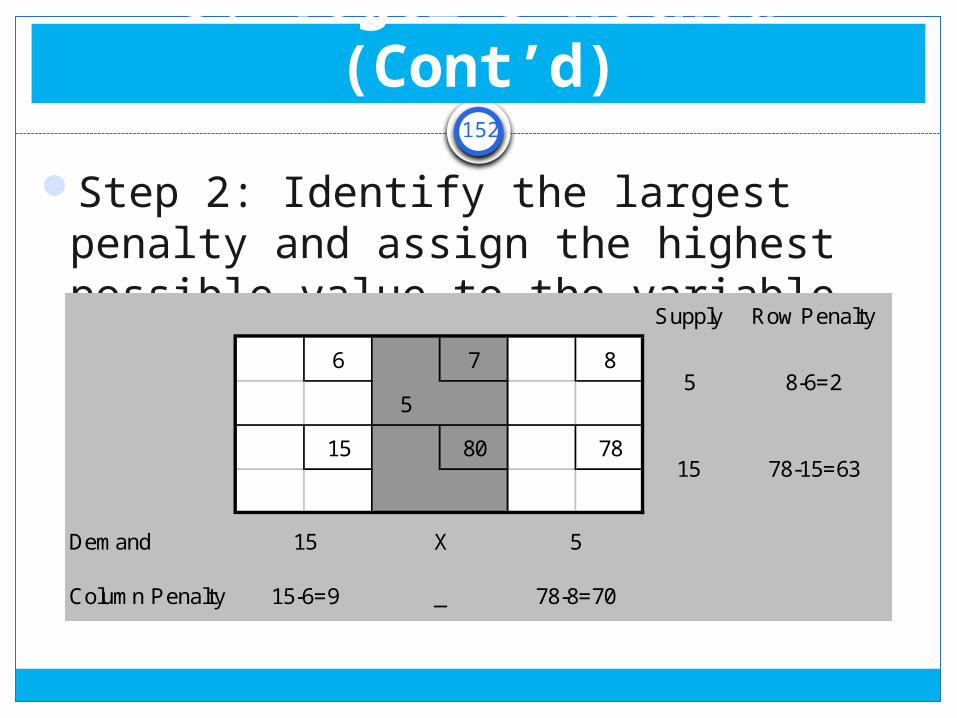
152
3. Vogel’s Method (Cont’d)
Step 2: Identify the largest penalty and assign the highest possible value to the variable.
Supply Row Penalty
6 7 8
5
15 80 78
Demand
Column Penalty 15-6=9 _ 78-8=70
8-6=2
78-15=63
15 X 5
5
15

153
3. Vogel’s Method (Cont’d)
Step 3: Identify the largest penalty and assign the highest possible value to the variable.
Supply Row Penalty
6 7 8
5 5
15 80 78
Demand
Column Penalty 15-6=9 _ _
_
_
15 X X
0
15

154
3. Vogel’s Method (Cont’d)
Step 4: Identify the largest penalty and assign the highest possible value to the variable.
Supply Row Penalty
6 7 8
0 5 5
15 80 78
Demand
Column Penalty _ _ _
_
_
15 X X
X
15

155
3. Vogel’s Method (Cont’d)
Step 5: Finally the BFS is found as X11=0, X12=5, X13=5, and X21=15
Supply Row Penalty
6 7 8
0 5 5
15 80 78
15
Demand
Column Penalty _ _ _
_
_
X X X
X
X

156
Improving the Obtained Solution
1. Determine the entering variable: Using the method of multipliers. Calculate the multipliers u & v, where:
Values of the multipliers can be determined from this relation by assuming an arbitrary value for any one of them.
For each non-basic variable , calculating
The entering variable is then selected as the one with the most positive

157
Improving the Obtained Solution (Cont’d)
x11: u1 + v1 = c11 = 10
x12: u1 + v2 = c12 = 0
x22: u2 + v2 = c22 = 7
x23: u2 + v3 = c23 = 9
x24: u2 + v4 = c24 = 20
x34: u3 + v4 = c34 = 18
1 2 3 4
1 5 10 15
2 5 15 5 25
3 5 5
5 15 15 10
1. Determine the entering variable:
For the opposite table, the equations associated with the basic variables are given as:
By letting u1 = 0, the values of the multipliers are successively determined as v1 = 10, v2 = 0, u2 = 7, v3 = 2, v4 = 13, and u3 = 5.

158
Improving the Obtained Solution (Cont’d)
1. Determine the entering variable: X31 has the most positive

159
Improving the Obtained Solution (Cont’d)
2. Determine the leaving variable (Loop construction):
A closed loop for the current entering variable is constructed.
The loop starts and ends at the designated non-basic variable.
It consists of successive horizontal and vertical (connected) segments whose end points must be basic variables, except for the end points that are associated with the entering variable.

160
Improving the Obtained Solution (Cont’d)
2. Determine the leaving variable (Loop construction):
This means that every corner element of the loop must be a cell containing a basic variable.
It is immaterial whether the loop is traced in a clockwise or counterclockwise direction.
In the example: This loop may be defined in terms of the basic
variables as X31 X11 X12 X22 X24 X34 X31

161
Improving the Obtained Solution (Cont’d)
1 2 3 4
1
10 0 20 11
155 10
– +
2
12 7 9 20
255 15 5
– +
3
0 14 16 18
5x31 5
+ –5 15 15 10

162
Improving the Obtained Solution (Cont’d)
2. Determine the leaving variable (Loop construction):
The leaving variable is selected from among the corner variables of the loop that will decrease when the entering variable X31 increases above the zero level.
These are indicated by the by the variables in the squares labeled with minus signs. In our particular problem, these variables are X11, X22, and X34.

163
Improving the Obtained Solution (Cont’d)
2. Determine the leaving variable (Loop construction):
The leaving variable is selected as the one having the smallest value, since it will be the first to reach zero value and any further decrease will cause it to be negative.
Since the three variables have the same value (=5), we arbitrarily select any of them as the leaving variable. Suppose that X34 is taken as the leaving variable, then the value of X31 is increased to 5, and the values of the corner basic variables are adjusted accordingly

164
Improving the Obtained Solution (Cont’d)
1 2 3 4
110 0 20 11
150 15
212 7 9 20
250 15 10
30 14 16 18
55
5 15 15 10

165
Improving the Obtained Solution (Cont’d)
3. Repeat the Previous Steps Till Optimality Is Reached:
The new basic solution should be checked for optimality by computing the new multipliers.
The previous steps should be repeated for each iteration.
The optimum solution is obtained when all the are non-positive.

166
Lecture 4 – B
The Transshipment Problem

167
The Transshipment Problem
It is a more general view of the transportation problem.
Not only is movement allowed from sources to sinks, but also: From sources to sources. From sinks to sinks. From sinks back to sources.
Costs are usually decreased, but problem size increases significantly.

168
Transportation Transshipment
Transportation vs. Transshipment
BB
AA
DD
EE
CC
BB
AA
DD
EE
CC

169
The Transshipment Matrix
To Source SinkAvailability
From 1…i…m 1…j…n1
(1)
Source-to-source sub-matrix
(2)
Source-to-sink sub-matrix
a1 + U
. .. .
Source i ai + U
. .
. .
m am + U
1
(3)
Sink-to-source sub-matrix
(4)
Sink-to-sink sub-matrix
U. .. .
Sink j U. .. .n U
Demand U … U … U b1 + U … bj + U … bn + U

170
The Transshipment Matrix (Cont’d)
Contains 4 main sub-matricies:1. source-to-source, 2. source-to-sink, 3. sink-to-source, 4. sink-to-sink.
All availabilities and demands include a constant U: the maximum amount that
could be transshipped

171
Transshipment Network Embedded Transportation Network
Transshipment Example
BB
AA
IIII
IIIIII
II
[20]
[7]
[9]
[9]
[9]
(12)
(14)
(10)
(6) (10)
(5)
(2)
(6)
(3) (3)
BB
AA
IIII
IIIIII
II
[20]
[7]
[9]
[9]
[9]
(12)
(14)
(10)
(6) (10)
(5)

172
Transshipment Example (Cont’d)
We shall first, for the purpose of comparison, solve for the solution to the embedded transportation problem.
I II III Available
A12 10 14
209 9 2
B6 10 5
77
Demand 9 9 9

173
Transshipment Example (Cont’d)
Then, we construct the transshipment matrix: To From
Source SinkAvailable
A B I II III
Source
A0 3 12 10 14
20 + 27
B3 0 6 10 5
7 + 27
Sink
I12 6 0 2 3
27
II10 10 2 0 6
27
III14 5 3 6 0
27
Demand 27 27 9 + 27 9 + 27 9 + 27

174
Transshipment Example (Cont’d)
Since , we have let U equal to 27 units.Next is to obtain initial feasible solution:
Could be achieved by VAM. Solution of the embedded transportation problem will
be used instead. Start by filling in the source-to-sink portion of the sub-
matrix (which is the embedded transportation matrix). Next, we allocate, to each main diagonal cell, the
amount U, which, for this problem, is 27 units.

175
Transshipment Example (Cont’d)
The resultant feasible initial allocation: To From
Source Sink
AvailableA B I II III
Source
A 270 3
912
910
214
47
B3
270 6 10
75
34
Sink
I12 6
270 2 3
27
II10 10 2
270 6
27
III14 5 3 6
270
27
Demand 27 27 36 36 36

176
Transshipment Example (Cont’d)
Next, solving the resultant matrix using the normal transportation technique.
Final transshipment solution: To From
Source SinkAvailable
A B I II III
Source
A 270
113 12
910 14
47
B3
160
96 10
75
34
Sink
I12 6
270 2 3
27
II10 10 2
270 6
27
III14 5 3 6
270
27
Demand 27 27 36 36 36

177
Transshipment Example (Cont’d)
Final solution representation:
BB
AA
IIII
IIIIII
II
[20]
[7]
[9]
[9]
[9]
11
9
9
9

178
Lecture 4 – C
The Assignment Problem

179
The Assignment Problem
The assignment problem is a special subclass of the transportation problem.
The assignment problem gets its name from a particular application in which we wish to assign "individuals" to "tasks (or tasks to machines, etc.).
It is assumed that each individual can be assigned to only one task, and each task is assigned to only one individual.

180
The Mathematical Model
Decision Variables:
Objective Function:
m = Number of source nodes (jobs, employees, etc.) n = Number of sink nodes (machines, offices, etc.) cij = Cost of assigning source i to sink j

181
The Mathematical Model (Cont’d)
Subject to:

182
The Assignment Problem Example
Machineco has four jobs to be completed. Each machine must be assigned to complete one job. The time required to setup each machine for completing each job is shown in the table below. Machinco wants to minimize the total setup time needed to complete the four jobs.

183
The Assignment Problem Example
Setup times(Also called the cost matrix)
Time (Hours)
Job1 Job2 Job3 Job4
Machine 1 14 5 8 7
Machine 2 2 12 6 5
Machine 3 7 8 3 9
Machine 4 2 4 6 10

184
The Model
According to the setup table Machinco’s problem can be formulated as follows (for i,j=1,2,3,4):
11 12 13 14 21 22 23 24
31 32 33 34 41 42 43 44
11 12 13 14
21 22 23 24
31 32 33 34
41 42 43 44
11 21 31 41
12 22 32 42
13 23
min 14 5 8 7 2 12 6 5
7 8 3 9 2 6 10
. . 1
1
1
1
1
1
Z X X X X X X X X
X X X X X X X X
s t X X X X
X X X X
X X X X
X X X X
X X X X
X X X X
X X
33 43
14 24 34 44
1
1
0 1ij ij
X X
X X X X
X or X

185
The Model
For the model on the previous page note that: Xij=1 if machine i is assigned to meet the demands of
job j Xij=0 if machine i is assigned to meet the demands of
job j In general an assignment problem is a balanced
transportation problem in which all supplies and demands are equal to 1.

186
Solution Method (Cont’d)
Although the transportation simplex appears to be very efficient, there is a certain class of transportation problems, called assignment problems, for which the transportation simplex is often very inefficient. For that reason there is an other method called The Hungarian Method.
Some basic ideas:1. Suppose we ranked all feasible assignments in
increasing order of cost.

187
Solution Method (Cont’d)
2. The ranking does not change if one subtracts the same amount, say, D, from all costs in the same row, since all assignment costs are reduced by D.
3. The ranking does not change if one subtracts the same amount, say, D, from all costs in the same column, since all assignment costs are reduced by D.
4. An assignment selects one entry in each row and one in each column.

188
Solution Method (Cont’d)
5. As long as all costs are kept nonnegative, if the reduced cost matrix allows a zero cost assignment, that assignment is optimal.
6. If there is a zero cost in each row and a zero cost in each column of the reduced cost matrix, this assignment is optimal.

189
Solution Method (Cont’d)
The steps of The Hungarian Method are as listed below: Step1: Find the minimum element in each row of the mxm cost
matrix. Construct a new matrix by subtracting from each cost the minimum cost in its row. For this new matrix, find the minimum cost in each column. Construct a new matrix (reduced cost matrix) by subtracting from each cost the minimum cost in its column.
Step 2: Draw the minimum number of lines (horizontal and/or vertical) that are needed to cover all zeros in the reduced cost matrix. If m lines are required , an optimal solution is available among the covered zeros in the matrix. If fewer than m lines are required, proceed to step 3.

190
Solution Method (Cont’d)
The steps of The Hungarian Method are as listed below: Step 3: Find the smallest nonzero element
(call its value k) in the reduced cost matrix that is uncovered by the lines drawn in step 2. Now subtract k from each uncovered element of the reduced cost matrix and add k to each element that is covered by two lines. Return to step 2.

191
Solving the Assignment Problem
Row reduction:
Time (Hours)
Job 1 Job 2 Job 3 Job 4
Machine 1 14-5 5-5 8-5 7-5
Machine 2 2-2 12-2 6-2 5-2
Machine 3 7-3 8-3 3-3 9-3
Machine 4 2-2 4-2 6-2 10-2

192
Solving the Assignment Problem
Time (Hours)
Job1 Job2 Job3 Job4
Machine 1 9 0 3 2-2
Machine 2 0 10 4 3-2
Machine 3 4 5 0 6-2
Machine 4 0 2 4 8-2
Column reduction:

193
Solving the Assignment Problem
Time (Hours)
Job1 Job2 Job3 Job4
Machine 1 9 0 3 0
Machine 2 0 10 4 1
Machine 3 4 5 0 4
Machine 4 0 2 4 6
Result of column reduction:

194
Solving the Assignment Problem
Time (Hours)
Job1 Job2 Job3 Job4
Machine 1 9+1 0 3+1 0
Machine 2 0 10-1 4 1-1
Machine 3 4 5-1 0 4-1
Machine 4 0 2-1 4 6-1
Crossing out zeros:

195
Solving the Assignment Problem
Time (Hours)
Job1 Job2 Job3 Job4
Machine 1 10 0 4 0
Machine 2 0 9 4 0
Machine 3 4 4 0 3
Machine 4 0 1 4 5
Crossing out zeros after modification:

196
Solving the Assignment Problem
Optimal AssignmentFor the Reduced Cost Matrix
Time (Hours)
Job1 Job2 Job3 Job4
Machine 1 10 0 4 0
Machine 2 0 9 4 0
Machine 3 4 4 0 3
Machine 4 0 1 4 5