orangutan distribution, density, abundance and impacts of ... · orangutan distribution, density,...

77

CHAPTER 6

Orangutan distribution, density, abundance and impacts of disturbanceSimon J. Husson, Serge A. Wich, Andrew J. Marshall, Rona D. Dennis, Marc Ancrenaz, Rebecca Brassey, Melvin Gumal, Andrew J. Hearn, Erik Meijaard, Togu Simorangkir and Ian Singleton

Photo © Perry van Duijnhoven

grinnel.indb 77grinnel.indb 77 11/24/2008 4:20:55 PM11/24/2008 4:20:55 PM

78 O R A N G U TA N S

6.2 Distribution

6.2.1 Historical distribution, dispersal and range contraction

The orangutan emerged as a distinct species

around 2–3 million years ago on the Asian main-

land, and dispersed southwards throughout South

East Asia and the Sundaland region (Steiper 2006).

Until 12,500 years ago, orangutans were distrib-

uted more or less continuously from the foothills

of the Himalaya mountain chain to the large Sunda

islands of Sumatra, Borneo and Java—a histor-

ical distribution covering at least 1.5 million km2

(Rijksen and Meijaard 1999). Environmental

changes (Jablonski et al. 2000), slash-and-burn agri-

culture and increasing hunting pressure reduced

their range, and since the seventeenth century the

orangutan has only occurred in the wild on the

islands of Borneo and Sumatra. Reliable records of

their distribution did not appear until the 1930s,

a comprehensive review of which can be found in

Rijksen and Meijaard (1999), and their complete

distribution was not satisfactorily known until the

beginning of the twenty-G rst century (Singleton et al. 2004).

Orangutans are believed to have entered south-

ern Borneo from Sumatra via the (now submerged)

Bangka–Belitung–Karimata land-bridge (Rijksen

and Meijaard 1999). They cannot cross wide rivers,

so they must have dispersed along Borneo’s cen-

tral mountain chain, traversing the headwaters of

the major rivers where they were narrow enough

to cross. In the center of Borneo is a mountainous

region where the Schwaner mountains meet the

Muller mountains and where Borneo’s three largest

rivers, the Barito, Mahakam and Kapuas, originate.

Orangutans that dispersed across the headwaters

of the Kapuas gave rise to the populations in west-

ern Borneo (West Kalimantan north of the Kapuas,

Sarawak, Brunei, and Sabah west of the Padas river)

and those that dispersed across the head waters of

the Mahakam resulted in the populations of eastern

and northern Borneo (East Kalimantan and Sabah

east of the Padas river). These dispersal routes

must have closed at some point, perhaps because

changes in sea-level and climate made the habitat

6.1 Introduction

Knowledge of a species’ distribution, density

and population size is essential for conservation,

because collecting this information is the only

adequate method of assessing a species risk of

extinction. As the Sumatran orangutan is con-

sidered critically endangered (Singleton et al. 2007) and the Bornean orangutan endangered

(Ancrenaz et al. 2007) it is important to obtain

distribution and density data for all orangutan

populations. In this chapter we provide a concise

overview of orangutan distribution and density.

In addition to being essential for orangutan con-

servation, these data also serve as the basis for

studies investigating variation in forest produc-

tivity and the effects it might have on orangutan

density (Chapter 7).

Earlier studies on orangutan density have gen-

erally suggested that Sumatran orangutans are

found at higher densities than Bornean orangutans

(Rijksen and Meijaard 1999); that orangutan density

declines with increasing altitude (Djojosudharmo

and van Schaik 1992; Rijksen and Meijaard 1999)

and that it is negatively impacted by logging (Rao

and van Schaik 1997; Morrogh-Bernard et al. 2003;

Felton et al. 2003; Johnson et al. 2005b). Because the

orangutan is a frugivore, variation in fruit avail-

ability is thought to be the main cause of these

variations in density. Fruit availability is higher

in Sumatra than Borneo (Chapter 7), declines with

altitude on both islands (Djojosudharmo and van

Schaik 1992; Cannon et al. 2007) and is reduced

by logging (Johns 1988; Grieser Johns and Greiser

Johns 1995).

These earlier studies have been limited to

comparisons between a small number of sites,

however, and have often not taken into account

variation in survey methods between the sites

under comparison. In this chapter we reinves-

tigate these hypotheses/results, armed with the

largest set of density estimates yet available, and

attempt to standardize for differences in G eld

survey methods and the parameters used to

convert nest-density data to orangutan density

estimates.


O R A N G U TA N D I S T R I B U T I O N , D E N S I T Y, A B U N D A N C E A N D I M PA C T S O F D I S T U R B A N C E 79

oil, tobacco and rubber, began during the colonial

period and has become a major source of revenue

for Indonesia and Malaysia. In Sumatra, most of

the forests surrounding Lake Toba have been con-

verted to plantation, and there has been consider-

able encroachment and forest clearance all around

the Leuser Ecosystem, notably in the Alas Valley,

Bengkung, Deli and Langkat regions. In the orang-

utan’s Bornean range, the lowland forests of the

Kapuas basin in West Kalimantan were more or

less cleared during the twentieth century for agri-

culture and commercial logging. Large oil palm

plantations have been established in most of the

lowland area between the Sampit river in Central

Kalimantan and Gunung Palung National Park in

West Kalimantan. Oil palm has also been grown on

former forest land in much of the coastal regions of

Sabah and Sarawak. Large-scale forest G res have

occurred in much of eastern and southern Borneo,

resulting from drought, peatland drainage and

arson, so that there is now virtually no lowland

forest remaining in East Kalimantan south of the

Sangkulirang peninsula, or in south-east Central

Kalimantan between the Sabangau and Barito riv-

ers. The opening up of forest to logging concessions

has led to increased opportunities for hunting.

During the mid- to late-twentieth century this has

been as much for the pet trade as for meat or for

cultural reasons. It is likely that orangutans have

been hunted to extinction in areas of forest that

naturally supported low orangutan densities, such

as in the Schwaner mountains around the head-

waters and tributaries of the Katingan and Barito

rivers, and in most of the Barisan mountain chain

in Sumatra.

6.2.2 Current distribution

Orangutan distribution in 2003 was described at the

Jakarta Orangutan Population and Habitat Viability

Analysis Workshop (Singleton et al. 2004). Using a

combination of ground and aerial G eld surveys,

LANDSAT and MODIS imagery and Indonesian

Ministry of Forestry data, Wich et al. (2008) identi-

G ed 306 separate forest blocks in Borneo and 12 in

Sumatra that potentially contained orangutans in

in the hills unsuitable for orangutans, or because

of hunting or forest clearing by humans. Whatever

the reason, evidence suggests that these popula-

tions have remained separate from each other, and

from those in southern Borneo, for a considerable

period of time (Warren et al. 2001; Chapter 1) and

they are now classed as separate subspecies, Pongo pygmaeus pygmaeus in western Borneo, P. p. morio in eastern Borneo and P. p. wurmbii in southern

Borneo.

The headwaters of the Barito river appear to have

blocked orangutans from dispersing further along

the south of the Schwaner range, as there are few

records of the species occurring in and around

these headwaters (Rijksen and Meijaard 1999) and

the orangutan is virtually absent from the south-

east of Borneo, east of the Barito river and south of

the Mahakam river, despite the presence of appar-

ently suitable habitat in the region. The only excep-

tion is an isolated population between the Barito

and Negara rivers, G rst reported in the 1930s. This

small population is most likely the result of changes

in the course of the Barito river which separated

and then isolated a group of orangutans.

Orangutans once inhabited all suitable habitat

in Sumatra and Borneo, apart from the south-east

corner of Borneo, but by the end of the twentieth

century they had disappeared from many parts

of their former range. There are no reliable recent

records of orangutans in the north-west of Borneo

(Sarawak north of the Rajang River and the coastal

zones of Brunei and western Sabah); the Kayan–

Mentarang water catchment in East Kalimantan

or most of the eastern lowlands of Sumatra. These

regions are the traditional homes for several tribes

of hunter-gatherer peoples who probably hunted

the orangutan to extinction in these forests (Rijksen

and Meijaard 1999).

Nearly the entire remaining orangutan forest

habitat has been exploited in some way, as detailed

in Rijksen and Meijaard (1999). Large areas of

forest have been cleared, initially by indigenous

groups of shifting-cultivators, and more recently

to expand settlements, build transport links and

for growing food crops. International trade in

timber and agricultural products, including palm



of other habitats including heath forest (kerangas)

on sandy soils (Payne 1987; Galdikas et al. unpub-

lished data) and limestone-karst forest (Marshall et al. 2006, 2007), and they have also been recorded

in Nypa palm stands and mangrove forest in

Sabah (Ancrenaz and Lackman-Ancrenaz 2004),

albeit at very low density. Orangutans are gen-

erally rare or absent at high altitudes (more than

500 m above sea level (asl) in Borneo and 1500m asl

in Sumatra; Rijksen and Meijaard [1999]). They are

thus rarely found in submontane and montane

forests, although the submontane (800–1000 m asl)

forest in Gunung Palung National Park occasion-

ally supports high densities of orangutan (Johnson et al. 2005b) and the highest density of orangutan

2002. Of these, 32 in Borneo and 6 in Sumatra sup-

port at least 250 individuals, the proposed mini-

mum viable population size (Singleton et al. 2004;

Chapter 22). Only 17 habitat blocks in Borneo and

3 in Sumatra support populations in excess of 1000

individuals. This distribution is shown in Figures

6.1 and 6.2.

Orangutans are found in dry lowland and

hill forests dominated by tree species from the

Dipterocarpaceae family; peat-swamp forest in

poorly drained river basins; and freshwater swamp

forest and alluvial forest in river valleys. These are

the prime habitats for orangutan, which provide

sufG cient food to support permanent populations

(Chapters 7–9). Orangutans also occur in a range

96°0'0"E 98°0'0"E

4°0'0"N

2°0'0"N

98°0'0"E96°0'0"E

2°0'0"N

4°0'0"N

N

50 25 0 50 Kilometers

Figure 6.1 Orangutan distribution in Sumatra (dark gray). Surveyed locations included in this analysis are marked with a boxed cross.



habitats it is likely that they are either dispersing

adult males (Delgado and van Schaik 2000) or

are able to utilize adjacent prime habitat types in

order to meet their nutritional requirements. For

example, the karst forests of the Sangkuliarang

peninsula are adjacent to mixed dipterocarp for-

est (Marshall et al. 2007) and the montane slopes

of Mount Palung rise steeply from the mixed dip-

terocarp and peat-swamp forests at its base. It is

nests in Mount Kinabalu National Park was found

between 800 and 1300 m asl in forest growing on

outcrops of igneous rock at the interface between hill

dipterocarp forest and montane forest (Ancrenaz

and Lackman-Ancrenaz 2004).

These marginal habitats provide less orang utan

food and it seems likely that large expanses of

these habitat types are unable to support perman-

ent populations. Where they do occur in marginal

110˚0'0"E

5˚0'0"N

0˚0'0"

5˚0'0"N

0˚0'0"

115˚0'0"E

110˚0'0"E 115˚0'0"E

N

0 75 150 300 Kilometers

Figure 6.2 Orangutan distribution in Borneo (dark gray). Surveyed locations included in this analysis are marked with a boxed cross. Dashed lines mark the boundaries between subspecies



Hypotheses 2: Orangutan density declines

with increasing altitude.

Density is reported to decline with altitude

(van Schaik et al. 1995; Rijksen and Meijaard

1999; Johnson et al. 2005b) and this is believed

to be a consequence of lower food availability at

higher altitudes, particularly of I eshy-pulp fruits

(Djojosudharmo and van Schaik 1992).

Hypotheses 3: Peat-swamp forest supports higher

densities than other habitat-types, followed by

dry forest and karst forest.

Marshall et al. (Chapter 7) conclude that the high-

est orangutan densities are found at sites with

shorter, less frequent and less extreme periods of

low food availability. This implies that peat-swamp

forests should support higher densities than dry

forest types, as dry forests experience extreme

temporal I uctuations in food availability owing

to the mast-fruiting phenomenon (Leighton and

Leighton 1983; Knott 1998a), which exhibits peaks

of synchronized fruit production followed by

several years of reproductive inactivity (Medway

1972; Ashton et al. 1988). In contrast, peat-swamp

forest displays consistent reproductive productiv-

ity (Cannon et al. 2007), and so we hypothesize

that orangutan densities are highest in this habitat

type. We expect karst forests to support the lowest

densities, owing to their relatively low tree species

diversity and more limited productivity (Marshall et al. 2007).

Hypotheses 4: ‘Mosaic’ sites support higher

orangutan densities than single habitat types.

A further category of habitat in which we may

expect overall fruit availability to be high and peri-

ods of low-fruit availability to be short are ‘mosaic’

habitats. These are deG ned as areas in which all

or most individuals in a population have access

within their home ranges to two or more different

types of habitat, e.g. dry, dipterocarp-dominated,

forest with accumulations of peat in depressions,

or peat-swamp forest margins that are seasonally

inundated with river I oodwater. In such areas

one habitat may be more productive overall but

the other have a more stable, year-round supply

of food (Cannon et al. 2007), so that the orang-

utan population can exploit different habitats at

also possible that interfaces between two habitat

types, such as found at high altitudes on Mount

Kinabalu, provide suitable conditions for orang-

utan survival, where either on its own does not.

6.3 Density

6.3.1 Hypotheses

6.3.1.1 Habitat differencesSimple ecological theory suggests that a species’

density is positively correlated with the amount of

food available to it, and more speciG cally that den-

sity of slow-reproducing species (such as orang-

utans) are limited by the frequency and duration

of periods of food shortage (Cant 1980; Marshall

and Leighton 2006). In support of this, Marshall et al. (Chapter 7, using data from 12 sites) found

that Sumatran forests were better orangutan habi-

tat than Bornean forests, and that orangutan den-

sity was positively correlated with fruit abundance

during periods of low-fruit availability, indicating

that sites which experience less extreme periods

of food shortage can support higher densities.

Here we suggest basic hypoth eses that arise from

Marshall et al.’s conclusions, and test whether they

hold true for the larger sample of sites presented

here.

Hypotheses 1: Sumatran orangutans are found at

higher densities than Bornean orangutans.

Published orangutan densities in Sumatra are

consistently higher than estimates from compar-

able habitat in Borneo (Rijksen and Meijaard 1999;

Singleton et al. 2004) and this is generally assumed

to result from higher levels of plant productivity,

and hence greater availability of orangutan food,

on Sumatra’s more fertile volcanic soils (Rijksen

and Meijaard 1999). In Chapter 7, Marshall et al. G nd that Sumatran forests have a higher propor-

tion of stems bearing fruit; are more often in peri-

ods of high-fruit availability; have higher densities

of some of the orangutan’s preferred foods; and

experience shorter periods of low-fruit availability,

than in comparable habitats in Borneo. These G nd-

ings are all consistent with, and provide support

for, the assumption stated above. Hence we test the

hypothesis that Sumatran forests support higher

densities of orangutans.



majority of studies that have directly examined the

effect of logging on orangutan density support this

hypothesis (Rao and van Schaik 1997; Felton et al. 2003; Morrogh-Bernard et al. 2003; Johnson et al. 2005b), some studies G nd no obvious relationship

(Marshall et al. 2006), or that undisturbed areas of

habitat support similar densities to partly disturbed

areas (Ancrenaz et al. 2004b), or that populations

can recover to pre-logging density in a relatively

short-period of time (Knop et al. 2004). We test to

see if densities in unlogged forest are signiG cantly

higher than those in logged forest.

Hypotheses 7: There is a degree of logging

damage that can be tolerated by orangutans.

Little, or no, difference in orangutan density

between unlogged areas and areas of ‘light’ logging

have been found in some studies (Ancrenaz et al. 2004b, 2005; Marshall et al. 2006). The most prized

timber species are those from the Dipterocarpaceae

family, which are not regarded as important food

for primates, including orangutans (Chivers 1980;

Chapter 9). Therefore a well-managed, selective-

logging operation that only removes those spe-

cies of trees and does minimal damage to the

surrounding forest may not signiG cantly alter the

forest structure and food availability from an oran-

gutan’s perspective. We test to see if there are dif-

ferences in density between four classes of logging

disturbance.

Hypotheses 8: Logging operations lead to

inflated orangutan densities in neighboring,

unlogged habitat.

MacKinnon (1971) G rst observed that orangutans

exposed to disturbance move out of the local area,

returning once the disturbance is over. This dis-

placement of orangutans leads to what has been

described as ‘refugee crowding’, i.e. an overshoot of

the carrying capacity in forested areas that neigh-

bor areas where logging is active. InI ated dens ities

in such areas have been reported in a number of

studies in Borneo (Russon et al. 2001; Morrogh-

Bernard et al. 2003; Ancrenaz and Lackman-

Ancrenaz 2004; Marshall et al. 2006) although this

has not been observed in Sumatra where at least

adult females are unwilling to leave their home

ranges (van Schaik et al. 2001).

different times of year (Singleton and van Schaik

2001). Alternatively, the species composition of

each habitat may be different, with preferred food

species fruiting at different times of the year in the

two habitat types. In either case, from an orang-

utan’s perspective, there are likely to be fewer peri-

ods of low-fruit availability in ‘mosaic’ habitats

than in areas with only one type of habitat.

Hypotheses 5: Densities of P. pygmaeus morio are

lower than the other subspecies of P. p. pygmaeus

and P. p. wurmbii.Eastern Borneo experiences long periods of drought

(MacKinnon et al. 1996; Walsh and Newbery 1999)

and so we expect that forests in this region show

greater seasonality of food availability, and hence

longer periods of extreme food shortage, than else-

where in Borneo. Thus, we hypothesize that dens-

ities of P. p. morio will be lower than those of the

other two subspecies of Bornean orangutan, unless

the local populations have evolved special adapta-

tion to food scarcity (Taylor 2006a; Chapter 2).

6.3.1.2 Impacts of disturbanceHuman disturbances complicate our analyses in

a number of ways. By felling and removing large

trees, logging theoretically lowers the availability

of food and hence carrying capacity (Johns 1988;

Grieser Johns and Greiser Johns 1995), but also

affects the behavior, diet and ranging patterns of a

species (Johns 1986; Marsh et al. 1987; Rao and van

Schaik 1997; Meijaard et al. 2005). Additionally, log-

ging operations provide increased opportunities

for hunting (Rijksen and Meijaard 1999) which can

have strong negative impacts on orangutan popu-

lations (Leighton et al. 1995; Marshall et al. 2006).

Hypotheses 6: Orangutan density is

negatively correlated with the intensity

of logging damage.

Logging damages forest structure through the

removal of commercial timber species, inciden-

tal damage to other trees, lianas and G gs and the

construction of logging access routes. This inevit-

ably reduces the number of fruit-bearing trees,

and thus is likely to reduce the carrying capacity

of the habitat and orangutan density. Although the



and 50% range 0.91–3.09 ind km–2. All estimates

are presented in Table 6.2. It should be noted that

many study sites have been purposefully chosen

in areas of high density, and lower-density sites,

such as upland areas, non-mosaic peat-swamps

and karst forests, are under-represented in our

sample. Therefore the median density of our sam-

ple is likely to be higher than the overall median

orangutan density across the species full range.

The standardization process resulted in higher

6.3.2 Density estimates and accuracy of standardization

Estimates of orangutan density were collated from

studies in which nest-count survey methods were

used (Box 6.1) and standardized for differences in

study design (Box 6.2).

Standardized density estimates were in the range

0.06 individuals per square kilometer (ind km–2)

to 9.58 ind km–2 with a median of 1.93 ind km–2

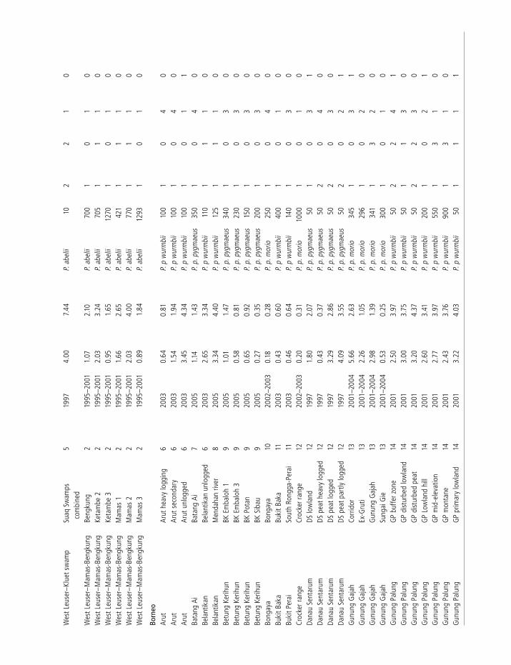
Survey data from a combination of published papers, survey reports and unpublished data are collated here. These are from 110 locations in 42 forest blocks, including 29 locations in 11 forest blocks for P. abelii; 9 locations in 3 forest blocks for P. p. pygmaeus; 37 in 16 forest blocks for P. p. morio and 35 in 12 forest blocks for P. p. wurmbii. All surveys were carried out since 1993.

At all sites orangutan density was estimated by counting orangutan nests (sleeping platforms) along straight-line transects, with the exception of sixteen sites in Sabah which were surveyed by helicopter. In the latter method the resulting aerial nest-counts were related to absolute nest density by calibrating with nest counts from concurrent ground surveys (see Ancrenaz et al. [2005b] for full details). In all cases the effective transect width was calculated using the Distance software program (Thomas et al. 2006) and nest density (DN) estimated accordingly. Nest densities are converted to orangutan density using the formula: DOU = DN/( p � r � t ) where: p = proportion of nest-builders in the population, r = number of nests built per day per individual, and t = nest decay time in days.

Each survey location was classifi ed for the following variables:

Species/subspecies:• Following the revised classifi cation of Groves (2001) and Brandon-Jones et al. (2004).

Dominant habitat type:• Three broad habitat types are described: (1) peat-swamp forest: forest growing on peat deposits, including both ombrotrophic (‘true’) peat-swamps (the only external source of water and nutrients is via aerial deposition from rain, aerosols and dust) and minerotrophic peat-swamps (which receive external supplies of water and nutrients from surface run-off, groundwater fl ow or seasonal inundation of river water);

(2) limestone–karst forest: dipterocarp-dominated forest growing on limestone bedrock, often with a dramatic landscape of pinnacles, sinkholes, caves and cliffs; (3) dryland forest: typically dipterocarp-dominated mast-fruiting forests on a wide range of soils, found in lowland plains and foothills, hilly regions and mountainsides.

‘Mosaic’ habitat• : whether more than one habitat type is present at or near to the study site.

Altitude:• in meters above sea level.Logging disturbance: • each site was classed as either

logged or unlogged. We further subdivided logged sites into lightly logged, logged or heavily logged, for cases where these divisions are made explicit in the literature, and recorded whether active logging was present in contiguous habitat adjacent to, but not in, each survey site. Classifications of logging intensity between sites in a single study is largely based on measurements of tree density, canopy disruption and stump density, and/or the visual determination of canopy structure and forest condition, although no empirical data exist to compare logging intensity between studies and thus there remains the possibility of bias.

These habitat characteristics are necessarily limited to broad defi nitions and thus we can only test for the presence of correlations without being able to identify the reasons for differences in density. Including more detailed site-specifi c variables, for example stem density, stand biomass and fruit availability, would greatly increase the power of our analyses, but these data are only available for a handful of sites, some of which are considered separately in Chapter 7. Nevertheless, we can assess whether the conclusions of Chapter 7 and other similar studies support or contrast with trends from this larger dataset.

Box 6.1 Survey methods



In order to properly compare densities between different habitat types and locations, these results have been standardized to control for the effects of different survey techniques. There is much variation in the values used for the nest-life history parameters and so we have recalculated densities using standardized values. These values are shown in Table 6.1. p has been estimated by direct observation at six sites and is similar at all sites, so the mean value of 0.89 is used. r has been estimated by direct observation at the same six sites and is distinctly higher in Sumatra compared to Borneo.

A lower r value was estimated at Lower Kinabatangan than at the three sites in southern Borneo, refl ecting a higher-than-normal incidence of nest reuse at Lower Kinabatangan (Ancrenaz et al. 2004a). This may be common to the P. p. morio sub-species or could have arisen in Lower Kinabatangan owing to heavy habitat disturbance and consequent overcrowding of the population there, meaning that there are relatively few potential nest sites. In the absence of data from other sites in P. p. morio’s range we have decided to use the value of 1.0 nests/day/individual for Lower Kinabatangan only and a mean value of 1.16 for all other sites in Borneo. For Sumatra a mean value of 1.80 is used.

There is greatest inter-site variation in t, the nest decay time. The time taken for a nest to decay is likely to (a) be positively correlated with climatic factors such

as temperature, rainfall, humidity and wind (van Schaik et al. 1995; Mathewson et al. 2008); b) depend on nest building-time and complexity (night nests last longer than day nests, which are generally built more quickly and are thus less sturdy); and (c) depend on the wood density of the trees used to build the nest (harder/denser wood, such as that of the Dipterocarpaceae family, decays slower; Ancrenaz et al. 2004a; Mathewson et al. 2008). Soil pH is thought to be a good proxy for wood density (Buij et al. 2003), as wood is denser and thus stronger on acidic soils (van Schaik and Mirmanto 1985). One study has suggested that nest decay rates are positively correlated with altitude in Sumatra (van Schaik et al. 1995) although others in Sumatra (Buij et al. 2003; Wich unpublished data) and Borneo (Johnson et al. 2005b; Marshall et al. 2006) have not found this relationship. Altitude correlates with temperature, and thus to some degree tree species composition and humidity, but not with other abiotic factors. While it may be possible to build a model to estimate t that incorporates all of these factors, these parameters are not known for most of the sites surveyed and the size of their effect on t is not fully understood. Therefore, for our purpose of standardizing density estimates, we control only those factors for which we have a good understanding, i.e. shorter decay rates in Sumatra compared to Borneo (higher incidence of day-nest construction in Sumatra), longer decay rates in

Box 6.2 Standardization of density estimates

Table 6.1 Nest ‘life history’ parameters estimated at eight sites in Sumatra and Borneo

Island Site Habitat p r t

Borneo Gunung Palung DF 0.89 1 1.16 1 259 1

Gunung Palung PSF – – 399 1

Lower Kinabatangan DF 0.85 2 1.00 2 202 2

Sabangau PSF 0.89 3 1.17 3 365 4

Mawas–Tuanan PSF 0.88 5 1.15 5 –Muara Lesan DF – – 602 * 6

Sumatra West Leuser–Ketambe DF 0.90 7 1.70 7 170 8

Kluet–Suaq PSF 0.90y9 1.90 9 199 10

Habitat: DF, Dry forest; PSF, Peat-swamp forest.

* Markov chain analysis.1 Johnson et al. 2005b; 2 Ancrenaz et al. 2004a; 3 Morrogh-Bernard unpublished data; 4 Husson unpublished data; 5 van Schaik et al. 2005a; 6 Mathewson et al. 2008; 7 van Schaik et al. 1995; 8 Wich unpublished data; 9 Singleton 2000; 10 Buij et al. 2003 (mean of backswamp and transit–swamp values).

continues



acidic peat-swamp forests than other habitat-types and longer decay rates on the east coast of Borneo–which has lower rainfall and is more drought-prone than the rest of the island (MacKinnon et al. 1996; Walsh and Newbery 1999).

t has been estimated at seven sites by following a cohort of nests from construction to disappearance. For Sumatra, values of 170 days for dryland forests and 193 days for peat-swamp forest are used. For Borneo peat-swamp forest, the value from Sabangau of 365 days is used in favor of that from Gunung Palung as the latter is based on a much smaller sample (35 nests vs 908 nests). For Borneo dryland forest, the value from Gunung Palung of 259 days is used in favor of that from Lower Kinabatangan as the latter is from a shorter period of study (2 years 4 months vs 5 years). Nest decay rates in dry forest sites in East Kalimantan are very slow, however (Mathewson et al. 2008), which can be attributed to lower annual rainfall on the east coast of Borneo compared to the rest of the island, and thus we use a value of 602 days for sites in East Kalimantan.

Once density estimates were standardized for differences in parameter values, they were corrected further for differences in survey technique. Surveys in which a transect is surveyed twice by different teams of observers obtain higher nest counts and higher nest density estimates than surveys in which transects are surveyed once only. Five separate studies indicate that densities obtained using the repeat survey method are higher by factors of 1.10–1.22 (Johnson et al. 2005b; van Schaik et al. 2005; Marshall et al. 2006; Husson unpublished data; Simorangkir unpublished data). Two studies have shown that nest densities obtained by counting nests in plots are higher by a factor of c. 1.25 than repeated line transect surveys (van Schaik et al. 2005; Husson unpublished data), and orangutan densities estimated this way closely approximate ‘real’ densities (van Schaik et al. 2005). Hence, a mean correction factor of 1.18 was applied to all data obtained by single surveys (including aerial survey data that was calibrated against single surveys on the ground), and a further correction factor of 1.25 applied to all data.

Box 6.2 continued

estimates than the original value in 83 cases and

lower estimates in the remaining 27. The stand-

ardized density was within 30% of the original

estimate in 35 of the 110 cases, and was over 80%

higher than the original estimate in 12 cases.

In order to judge the effectiveness of the nest sur-

vey method and this standardization process, these

estimates were compared to the actual density at

those sites where long-term studies have taken

place. Density estimates generated in this study

closely approximate those estimated from long-

term studies at G ve of the six sites where compa-

rable data are available (Table 6.3). The exception is

Ketambe in West Leuser, at which orangutan den-

sities exceeding 5 ind km–2 are regularly reported

by long-term researchers (Rijksen 1978; van Schaik et al. 1995, 2001) even though recent nest-survey

density estimates are invariably lower (Buij et al. 2003; Wich et al. 2004a).

This difference is unlikely to be due to either

survey error (the survey teams in Ketambe are

very experienced) or the standardization process

(which increased the published estimate). It seems

more likely that the Ketambe study site, a very fer-

tile area with high densities of strangling G gs (an

important fallback food resource; Wich et al. 2006a),

attracts large seasonal aggregations of apes (Rijksen

1978; Sugardjito et al. 1987). If orangutans make

biased use of their home range to spend as much

time as possible in the Ketambe study site during

periods of high-fruit abundance, then the estimate

of annual average density for this site will exceed

the actual density for the wider Ketambe region.

Nest counts along long, straight-line transects are

more likely to give a better estimate of density in

areas where there is markedly biased use of home

ranges, as randomly sited transects are predicted

to pass through both preferred and non-preferred

areas with equal frequency.

We must raise a note of caution before proceed-

ing. Although we show here that, in the majority

of cases, density estimates generated from nest

count surveys and this standardization closely

match ‘real’ densities at a number of sites, it must



also be noted that the estimation of parameters has

been most thorough at these same sites. Assigning

parameter values from one site to another, par-

ticularly the nest decay time t, remains the lar-

gest source of potential error (e.g. Mathewson et al. 2008). The plot method has not been validated for

habitats other than peat-swamp forest, and thus

the correction factor may not apply equally across

all habitats. The uncertainties generated by these

sources of error have led some researchers to calcu-

late nest density only. While this is perfectly valid

for comparisons within a site, nest densities are

affected by nest construction rates and decay rates,

so we have deemed it better to try and identify dif-

ferences in these parameters instead of ignoring

them. Nevertheless there is still more that can be

done to improve our estimates of t, in particular the

need to factor in effects of altitude, pH and rainfall.

At present, adequate data on these are lacking.

6.3.3 Results of analysis

Before proceeding with the analyses, we log �

1 transformed all density values as these were

highly skewed. To compare absolute densities for a

single independent variable we used independent-

samples t-tests or one-way ANOVA followed by

Tukey HSD post-hoc tests. All our tests are one-

tailed as our hypotheses are directional, and all

P-values are presented as such, with the exception

of non-directional hypothesis H5 for which two-

tailed P-values are presented.

Hypotheses 1: The G rst hypothesis, that densities

in Sumatra are higher than in Borneo, was sup-

ported when comparing all sites on the two islands

(t � 2.22, df � 108, p � 0.014). This difference was

especially strong when comparing peat-swamp

forest sites only (t � 3.20, df � 21, p � 0.002), but

was much reduced when comparing non-karst dry

forest sites (t � 1.42, df � 81, p � 0.080). The differ-

ence in density between the two islands appears

to be strongly inI uenced by higher densities in

Sumatran peat-swamp forest compared to Bornean

peat-swamp forest.

Hypotheses 2: We found no correlation between

density and altitude when comparing all sites (r �

–0.11, n � 110, p � 0.135), all dry forest sites (r �

–0.04, n � 83, p � 0.353), all Sumatran sites

(r � –0.24, n � 29, p � 0.103) or all Sumatran dry

forest sites (r � 0.57, n � 26, p � 0.783). We found

a strong signiG cant negative correlation between

density and altitude when comparing all Bornean

sites (r � –0.38, n � 81, p �0.0005) and all Bornean

non-karst dry forest sites (r � –0.39, n � 57, p �

0.002). Therefore we G nd that density declines sig-

niG cantly with increasing altitude in Borneo but

not in Sumatra.

Hypotheses 3: We hypothesized that densities

would vary between habitat types, with peat-

swamp forests expected to support the highest

densities, and karst forests the lowest. With all sites

included, mean values were in the expected order

of peat-swamp dry forest karst. Karst forest

supports signiG cantly lower densities than both

peat-swamp and dry forest but there is only a very

weak difference between peat-swamp and dry for-

est (F2, 107 � 7.13, p � 0.001; peat-swamp karst, p �

0.001; dry forest karst, p � 0.005; peat-swamp

dry forest, p � 0.052). Within each island the rank

order remained the same (there are no Sumatran

karst sites in our sample), although in Sumatra

peat-swamp density was signiG cantly higher than

density in dry forest (t � 2.94, df � 27, p � 0.003).

Differences in Borneo mirrored those for the full

sample.

Hypotheses 4: Our hypothesis that mosaic sites

support higher densities than non-mosaic sites

was strongly supported for all sites (t � 5.91, df

� 108, p �0.0005), Sumatra only (t � 2.70, df �

27, p � 0.006) and Borneo only (t � 6.25, df � 79,

p �0.0005). It seemed plausible that high densities

in mosaic habitats were strongly inI uencing our

previous test comparing between habitat types,

and so we reassigned each mosaic site to one of

three new habitat categories: (1) Peat-mosaic: pre-

dominately peat-swamp with dry or freshwater

habitats (essentially minerotrophic peat-swamps);

(2) Dry lowland-mosaic: predominately dry forest

with riverine/swamp habitats; (3) Hillside-mosaic:

dry forest sites with sharply changing altitudes

(essentially mountainsides).

Re-running the comparison showed signiG cant

differences between habitat types (F5, 104 � 9.85,

p �0.0005) and clearly separated the six habitat-

types into two groups, mosaic (mean values: peat-

mosaic dry lowland-mosaic hillside-mosaic)


Tabl

e 6.

2 De

nsity

est

imat

es a

nd s

ite d

escr

iptio

ns o

f 110

loca

tions

use

d in

this

anal

ysis

Hab

itat

uni

tRe

gion

nam

eRe

fere

nce

Surv

ey

date

(s)

Repo

rted

de

nsit

y (in

d/km

2 )

Stan

dard

ized

de

nsit

y (in

d/km

2 )

Spec

ies

Mea

n al

titu

de

(m)

Dom

inan

t ha

bita

tM

osai

cLo

ggin

g st

atus

Nei

ghbo

urin

g lo

ggin

g

Sum

atra

Bata

ng T

oru

Bata

ng T

oru

120

031.

142.

08P.

abe

lii50

01

02

0Ba

tang

Tor

uTe

luk

Nau

li1

2003

1.26

2.30

P. a

belii

850

10

21

East

Leu

ser–

Kapi

and

Upp

er

Lest

enAu

nan

219

95–2

001

1.63

3.26

P. a

belii

1036

10

10

East

Leu

ser–

Kapi

and

Upp

er

Lest

enBa

lailu

tu2

1995

–200

10.

571.

16P.

abe

lii91

61

01

0

East

Leu

ser–

Kapi

and

Upp

er

Lest

enKa

pi 1

219

95–2

001

0.52

0.97

P. a

belii

1236

10

10

East

Leu

ser–

Kapi

and

Upp

er

Lest

enKa

pi 2

219

95–2

001

0.61

1.14

P. a

belii

1266

10

10

East

Leu

ser–

Kapi

and

Upp

er

Lest

enM

arpu

nga

12

1995

–200

12.

624.

45P.

abe

lii92

51

01

0

East

Leu

ser–

Kapi

and

Upp

er

Lest

enM

arpu

nga

22

1995

–200

12.

794.

74P.

abe

lii11

221

01

0

East

Leu

ser–

Kapi

and

Upp

er

Lest

enM

arpu

nga

32

1995

–200

10.

300.

62P.

abe

lii11

001

01

0

East

Leu

ser–

Law

e Si

gala

-gal

aBa

tu 2

002

1995

–200

10.

280.

57P.

abe

lii12

831

01

0Ea

st L

euse

r–La

we

Siga

la-g

ala

Sele

dok

219

95–2

001

0.23

0.43

P. a

belii

1205

10

10

East

Leu

ser–

Siku

ndur

-Lan

gkat

Boho

rok

219

95–2

001

0.88

1.79

P. a

belii

500

10

10

East

Leu

ser–

Siku

ndur

-Lan

gkat

Siku

ndur

219

95–2

001

1.04

1.79

P. a

belii

501

01

0Ea

st L

euse

r–Si

kund

ur-L

angk

atTa

nkah

an2

1995

–200

10.

791.

58P.

abe

lii35

01

01

0Ea

st M

iddl

e Ac

ehSa

mar

kila

ng 1

219

95–2

001

1.14

2.09

P. a

belii

250

10

10

East

Mid

dle

Aceh

Sam

arki

lang

22

1995

–200

10.

410.

79P.

abe

lii75

01

01

0Tr

ipa

swam

pTr

ipa

319

932.

854.

20P.

abe

lii10

22

30

Trum

on-S

ingk

il sw

amp

Trum

on-S

ingk

il3

1993

4.00

5.90

P. a

belii

102

23

0W

est L

euse

r–Ea

st M

ount

Leu

ser/

Kem

iriAg

usan

219

95–2

001

5.99

10.1

8P.

abe

lii11

861

01

0

Wes

t Leu

ser–

East

Mou

nt L

euse

r/Ke

miri

Keda

h2

1995

–200

13.

796.

44P.

abe

lii14

561

01

0

Wes

t Leu

ser–

East

Mou

nt L

euse

r/Ke

miri

Kem

iri2

1995

–200

13.

124.

49P.

abe

lii11

831

01

0

Wes

t Leu

ser–

Klue

t hig

hlan

dsSu

aq H

ills

419

971.

572.

32P.

abe

lii50

10

10


Wes

t Leu

ser–

Klue

t sw

amp

Suaq

Sw

amps

co

mbi

ned

519

974.

007.

44P.

abe

lii10

22

10

Wes

t Leu

ser–

Mam

as-B

engk

ung

Beng

kung

219

95–2

001

1.07

2.10

P. a

belii

700

10

10

Wes

t Leu

ser–

Mam

as-B

engk

ung

Keta

mbe

22

1995

–200

12.

033.

24P.

abe

lii70

51

11

0W

est L

euse

r–M

amas

-Ben

gkun

gKe

tam

be 3

219

95–2

001

0.95

1.65

P. a

belii

1270

10

10

Wes

t Leu

ser–

Mam

as-B

engk

ung

Mam

as 1

219

95–2

001

1.66

2.65

P. a

belii

421

11

10

Wes

t Leu

ser–

Mam

as-B

engk

ung

Mam

as 2

219

95–2

001

2.03

4.00

P. a

belii

770

11

10

Wes

t Leu

ser–

Mam

as-B

engk

ung

Mam

as 3

219

95–2

001

0.89

1.84

P. a

belii

1293

10

10

Born

eoAr

utAr

ut h

eavy

logg

ing

620

030.

640.

81P.

p w

urm

bii

100

10

40

Arut

Arut

sec

onda

ry6

2003

1.54

1.94

P. p

wur

mbi

i10

01

04

0Ar

utAr

ut u

nlog

ged

620

033.

454.

34P.

p w

urm

bii

100

10

11

Bata

ng A

iBa

tang

Ai

720

051.

141.

43P.

p. p

ygm

aeus

350

10

40

Bela

ntik

anBe

lant

ikan

unl

ogge

d6

2003

2.65

3.34

P. p

wur

mbi

i11

01

11

0Be

lant

ikan

Men

daha

n riv

er8

2005

3.34

4.40

P. p

wur

mbi

i12

51

11

0Be

tung

Ker

ihun

BK E

mba

loh

19

2005

1.01

1.47

P. p

. pyg

mae

us34

01

03

0Be

tung

Ker

ihun

BK E

mba

loh

39

2005

0.58

0.81

P. p

. pyg

mae

us23

01

03

0Be

tung

Ker

ihun

BK P

otan

920

050.

650.

92P.

p. p

ygm

aeus

150

10

30

Betu

ng K

erih

unBK

Sib

au9

2005

0.27

0.35

P. p

. pyg

mae

us20

01

03

0Bo

ngay

aBo

ngay

a10

2002

–200

30.

180.

28P.

p. m

orio

250

10

40

Buki

t Bak

aBu

kit B

aka

1120

030.

430.

60P.

p w

urm

bii

400

10

10

Buki

t Per

aiSo

uth

Rong

ga-P

erai

1120

030.

460.

64P.

p w

urm

bii

140

10

30

Croc

ker r

ange

Croc

ker r

ange

1220

02–2

003

0.20

0.31

P. p

. mor

io10

001

01

0Da

nau

Sent

arum

DS lo

wla

nd12

1997

1.80

2.07

P. p

. pyg

mae

us50

10

31

Dana

u Se

ntar

umDS

pea

t hea

vy lo

gged

1219

970.

430.

37P.

p. p

ygm

aeus

502

04

0Da

nau

Sent

arum

DS p

eat l

ogge

d12

1997

3.29

2.86

P. p

. pyg

mae

us50

20

30

Dana

u Se

ntar

umDS

pea

t par

tly lo

gged

1219

974.

093.

55P.

p. p

ygm

aeus

502

02

1G

unun

g G

ajah

Corr

idor

1320

01–2

004

5.66

2.63

P. p

. mor

io34

51

03

1G

unun

g G

ajah

Ex-G

ruti

1320

01–2

004

2.26

1.05

P. p

. mor

io29

61

02

0G

unun

g G

ajah

Gun

ung

Gaj

ah13

2001

–200

42.

981.

39P.

p. m

orio

341

13

20

Gun

ung

Gaj

ahSu

ngai

Gie

1320

01–2

004

0.53

0.25

P. p

. mor

io30

01

01

0G

unun

g Pa

lung

GP

buffe

r zon

e14

2001

2.50

3.97

P. p

wur

mbi

i50

22

41

Gun

ung

Palu

ngG

P di

stur

bed

low

land

1420

013.

003.

75P.

p w

urm

bii

501

13

0G

unun

g Pa

lung

GP

dist

urbe

d pe

at14

2001

3.20

4.37

P. p

wur

mbi

i50

22

30

Gun

ung

Palu

ngG

P Lo

wla

nd h

ill14

2001

2.60

3.41

P. p

wur

mbi

i20

01

02

1G

unun

g Pa

lung

GP

mid

-ele

vatio

n14

2001

2.77

3.97

P. p

wur

mbi

i55

01

31

0G

unun

g Pa

lung

GP

mon

tane

1420

012.

433.

76P.

p w

urm

bii

900

13

10

Gun

ung

Palu

ngG

P pr

imar

y lo

wla

nd14

2001

3.22

4.03

P. p

wur

mbi

i50

11

11


Gun

ung

Palu

ngG

P pr

imar

y pe

at14

2001

4.09

5.59

P. p

wur

mbi

i50

22

11

Katin

gan

flood

plai

nsKa

t Kaj

ang

Pam

ali

1520

031.

951.

92P.

p w

urm

bii

102

22

0Ka

tinga

n flo

odpl

ains

Kat K

alur

uan

1520

020.

940.

93P.

p w

urm

bii

102

04

0Ka

tinga

n flo

odpl

ains

Kat P

erig

i15

2002

2.94

2.89

P. p

wur

mbi

i10

22

10

Katin

gan

flood

plai

nsKa

t Tar

anta

ng11

2003

1.69

1.66

P. p

wur

mbi

i10

20

30

Kuam

utKu

amut

1020

02–2

003

0.06

0.09

P. p

. mor

io50

01

03

0Ku

lam

baKu

lam

ba10

2002

–200

32.

503.

85P.

p. m

orio

100

11

31

Low

er K

inab

atan

gan

Gom

anto

ng F

R16

2002

–200

33.

803.

23P.

p. m

orio

100

11

10

Low

er K

inab

atan

gan

Low

er K

inab

atan

gan

Lot 1

1620

02–2

003

6.00

4.95

P. p

. mor

io10

01

13

0

Low

er K

inab

atan

gan

Low

er K

inab

atan

gan

Lot 1

0a16

2002

–200

31.

801.

83P.

p. m

orio

100

11

30

Low

er K

inab

atan

gan

Low

er K

inab

atan

gan

Lot 1

0b16

2002

–200

32.

402.

30P.

p. m

orio

100

11

40

Low

er K

inab

atan

gan

Low

er K

inab

atan

gan

Lot 2

1620

02–2

003

5.00

7.04

P. p

. mor

io10

01

13

0

Low

er K

inab

atan

gan

Low

er K

inab

atan

gan

Lot 3

1620

02–2

003

1.90

1.83

P. p

. mor

io10

01

13

0

Low

er K

inab

atan

gan

Low

er K

inab

atan

gan

Lot 4

1620

02–2

003

3.10

2.73

P. p

. mor

io10

01

13

0

Low

er K

inab

atan

gan

Low

er K

inab

atan

gan

Lot 5

1620

02–2

003

2.10

2.00

P. p

. mor

io10

01

13

0

Low

er K

inab

atan

gan

Low

er K

inab

atan

gan

Lot 6

1620

02–2

003

2.10

1.95

P. p

. mor

io10

01

13

0

Low

er K

inab

atan

gan

Low

er K

inab

atan

gan

Lot 7

1620

02–2

003

1.30

1.20

P. p

. mor

io10

01

14

0

Low

er K

inab

atan

gan

Low

er K

inab

atan

gan

Lot 8

1620

02–2

003

0.70

0.58

P. p

. mor

io10

01

14

0

Low

er K

inab

atan

gan

Low

er K

inab

atan

gan

Lot 9

1620

02–2

003

1.60

1.32

P. p

. mor

io10

01

14

0

Low

er K

inab

atan

gan

Pang

ui F

R16

2002

–200

32.

602.

27P.

p. m

orio

100

11

10

Man

gkut

upBl

ock

B M

ain

Cana

l15

2001

0.67

0.78

P. p

wur

mbi

i20

20

31

Mar

ang-

Baai

Baai

1320

01–2

004

1.74

0.81

P. p

. mor

io43

53

04

0M

aran

g-Ba

aiM

aran

g13

2001

–200

40.

390.

18P.

p. m

orio

125

30

40

Tabl

e 6.

2 (c

ont.)

Hab

itat

uni

tRe

gion

nam

eRe

fere

nce

Surv

ey

date

(s)

Repo

rted

de

nsit

y (in

d/km

2 )

Stan

dard

ized

de

nsit

y (in

d/km

2 )

Spec

ies

Mea

n al

titu

de

(m)

Dom

inan

t ha

bita

tM

osai

cLo

ggin

g st

atus

Nei

ghbo

urin

g lo

ggin

g


Maw

asTu

anan

1720

032.

773.

84P.

p w

urm

bii

202

24

0M

uara

Les

an/G

unun

g N

yapa

Gun

ung

Nya

pa13

2001

–200

40.

630.

29P.

p. m

orio

256

30

20

Mua

ra L

esan

/Gun

ung

Nya

paM

uara

Les

an13

2001

–200

46.

362.

96P.

p. m

orio

160

10

21

Pina

ngah

Pina

ngah

1020

02–2

003

0.23

0.35

P. p

. mor

io10

001

04

0Sa

bang

auLA

HG L

PF 1

996

1819

960.

961.

12P.

p w

urm

bii

102

01

0Sa

bang

auLA

HG M

SF 1

996

1819

962.

012.

35P.

p w

urm

bii

102

03

0Sa

bang

auLA

HG T

IF 1

996

1819

962.

132.

49P.

p w

urm

bii

102

01

0Sa

bang

auPa

ungg

ulas

1520

042.

703.

16P.

p w

urm

bii

102

23

1Sa

bang

au–K

ahay

anBl

ock

C Ka

lam

pang

an15

1999

0.42

0.49

P. p

wur

mbi

i10

20

31

Saba

ngau

–Kah

ayan

Bloc

k C

Pila

ng15

2000

1.13

1.31

P. p

wur

mbi

i10

20

31

Sam

ba–K

ahay

an u

plan

dsN

Kec

ubun

g15

2003

0.72

1.18

P. p

wur

mbi

i15

01

02

0Sa

mba

–Kah

ayan

upl

ands

N K

ecub

ung

a8

2005

1.10

1.59

P. p

wur

mbi

i17

81

03

0Sa

mba

–Kah

ayan

upl

ands

N K

ecub

ung

b8

2005

0.06

0.08

P. p

wur

mbi

i88

10

30

Sam

ba–K

ahay

an u

plan

dsS

Kecu

bung

820

051.

061.

48P.

p w

urm

bii

921

03

0Se

gam

aDa

num

Val

ley

1020

02–2

003

1.04

1.60

P. p

. mor

io25

01

01

0Se

gam

aSe

gam

a–Pr

oduc

tion

fore

sts

1020

02–2

003

1.30

2.00

P. p

. mor

io25

01

03

0

Sila

buka

nSi

labu

kan

1020

02–2

003

0.58

0.89

P. p

. mor

io25

01

03

1Ta

bin

Tabi

n10

2002

–200

31.

261.

94P.

p. m

orio

100

11

30

Tanj

ung

Putin

gTP

Cam

p Le

akey

1920

031.

962.

72P.

p w

urm

bii

102

21

0Ta

njun

g Pu

ting

TP d

istur

bed

dry

fore

st19

2003

1.59

2.21

P. p

wur

mbi

i10

10

30

Tanj

ung

Putin

gTP

dist

urbe

d sw

amp

1920

031.

991.

96P.

p w

urm

bii

102

03

0Ta

njun

g Pu

ting

TP g

ood

dry

fore

st19

2003

2.09

2.90

P. p

wur

mbi

i10

10

11

Trus

Mad

iTr

us M

adi

1020

02–2

003

0.41

0.63

P. p

. mor

io10

001

03

0U

lu K

alum

pang

Ulu

Kal

umpa

ng10

2002

–200

30.

300.

46P.

p. m

orio

250

10

20

Ulu

Tun

gud

Ulu

Tun

gud

1020

02–2

003

0.04

0.06

P. p

. mor

io10

001

04

0U

pper

Kin

abat

anga

nDe

ram

akot

1020

02–2

003

1.50

2.31

P. p

. mor

io50

01

02

0U

pper

Kin

abat

anga

nLo

kan

1020

02–2

003

1.19

1.83

P. p

. mor

io50

01

02

0U

pper

Kin

abat

anga

nTa

ngku

lap

1020

02–2

003

0.62

0.95

P. p

. mor

io50

01

04

0U

pper

Kin

abat

anga

nTa

wai

1020

02–2

003

0.07

0.11

P. p

. mor

io50

03

01

0

1, W

ich

and

Geu

rts

unpu

blish

ed; 2

, Wic

h et

al.

2004

a; 3

, van

Sch

aik

et a

l. 20

01; 4

, Bui

j et a

l. 20

03; 5

, Sin

glet

on 2

000;

6, S

imor

angk

ir un

publ

ished

; 7, G

umal

unp

ublis

hed;

8, B

rass

ey u

npub

lishe

d; 9

, Anc

rena

z 20

06; 1

0, A

ncre

naz

et a

l. 20

05; 1

1, H

earn

and

Ros

s un

publ

ished

; 12,

Rus

son

et a

l. 20

01; 1

2, M

arsh

all e

t al.

2006

; 14,

John

son

et a

l. 20

05b;

15,

Hus

son;

Mor

rogh

-Ber

nard

; McL

ardy

and

D’A

rcy

unpu

blish

ed; 1

6,

Ancr

enaz

et a

l. 20

04; 1

7, v

an S

chai

k et

al.

2005

a; 1

8, M

orro

gh-B

erna

rd e

t al.

2003

; 19,

Gal

dika

s et

al.

unpu

blish

ed.

Dom

inan

t hab

itat:

1, d

ry fo

rest

; 2, p

eat-s

wam

p fo

rest

; 3, l

imes

tone

–kar

st fo

rest

.

Mos

aic:

0, s

ingl

e ha

bita

t-typ

e; 1

, dry

-low

land

mos

aic;

2, p

eat m

osai

c, 3

, upl

and

mos

aic.

Logg

ing

stat

us: 1

, unl

ogge

d; 2

, lig

htly

logg

ed; 3

, log

ged;

4, h

eavi

ly lo

gged

.

Nei

ghbo

ring

logg

ing:

1, p

rese

nt; 0

, abs

ent.



regression for all non-peat or karst sites and then

conducted a one-way ANOVA between subspecies

on the residuals. Again, this was not signiG cant

(F2, 54 � 1.69, p � 0.195) so we G nd no evidence for

densities varying between subspecies on Borneo.

To identify those factors which explain the most

variance in population density, we conducted

an ordinary least squares (OLS) regression with

orang utan population density as the dependent

variable, coding both species and the presence/

absence of a mosaic of habitats as dichotomous var-

iables and habitat type as a block of dummy vari-

ables. The signiG cance of these dummy variables

was assessed as a set using the F test for r2 change.

We examined a scatterplot of the standardized

residuals against the standardized predicted val-

ues which conG rmed that assumptions of linearity

and homogeneity of variance were met.

In this test both mosaic and species were highly

signiG cant correlates of orangutan density (pres-

ence of mosaic absence of mosaic; P. abelii

P.pygmaeus) whereas altitude was not (whole model:

adjusted r2 � 0.36, F5, 104 � 13.44, p �0.0005; Mosaic:

β � 0.47, t � 5.65, p �0.0005; Species: β � 0.35, t �

3.54, p �0.0005; Altitude: β � –0.12, t � –1.04, p �

0.151). Habitat-type was also a signiG cant predictor

of density (r2 change � 0.05, F-change2, 104 � 3.84,

2-tailed p � 0.025) although peat-swamp forest

density was not signiG cantly higher than dry for-

est density (β � 0.13, t � 1.46, p � 0.074). Both peat-

swamp and dry forest habitats had signiG cantly

and non-mosaic (mean values: peat-swamp dry

forest karst). Post-hoc tests showed no signiG -

cant pairwise comparisons within either group.

Between groups, peat-mosaic habitat supports

signiG cantly higher densities than all non-mosaic

sites (peat-mosaic peat-swamp, p � 0.001; peat-

mosaic dry forest, p �0.0005; peat-mosaic

karst, p �0.0005); dry-lowland mosaic supports

signiG cantly higher densities than dry forest (p

� 0.002) and karst (p � 0.001) sites; and hillside-

mosaic supports signiG cantly higher densities

than karst forest (p � 0.010). Comparisons using

solely Bornean sites yielded comparable patterns;

sample sizes were too small to permit an analysis

using solely Sumatran sites.

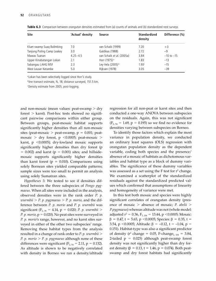
Hypotheses 5: We tested to see if densities dif-

fered between the three subspecies of Pongo pyg-maeus. When all sites were included in the analysis,

observed densities were in the rank order P. p. wurmbii P. p. pygmaeus P. p. morio, and the dif-

ference between P. p. morio and P. p. wurmbii was

signiG cant (F2, 78 � 4.14, p � 0.020; P. p. wurmbii

P. p. morio, p � 0.020). No peat sites were surveyed in

P. p. morio’s range, however, and no karst sites sur-

veyed in either of the other two subspecies’ range.

Removing these habitat types from the analysis

resulted in a change of rank order to P. p. wurmbii

P. p. morio P. p. pygmaeus although none of these

differences were signiG cant (F2, 54 � 2.11, p � 0.132).

As altitude is shown to be negatively correlated

with density in Borneo we ran a density/altitude

Table 6.3 Comparison between orangutan densities estimated from (a) counts of animals and (b) standardized nest surveys

Site ‘Actual’ density Source Standardized density

Difference (%)

Kluet swamp Suaq Balimbing 7.0 van Schaik (1999) 7.20 �3Tanjung Puting Camp Leakey 3.0 Galdikas (1988) 2.72 –9Mawas Tuanan 4.25–4.5 van Schaik et al. (2005a) 3.84 –10 to –15Upper Kinabatangan Lokan 2.1 Horr (1975) a 1.83 –13Sabangau LAHG MSF 2.3 Ley-Vela (2005) b 1.93c –15West Leuser Ketambe 5.0 Rijksen (1978) 3.05 –39

a Lokan has been selectively logged since Horr’s study.b line transect estimate, N, 18; distance surveyed, 151.5 km.c Density estimate from 2005, post-logging.



6.4 Discussion

6.4.1 Natural variation in orangutan density

In this chapter we have presented the G rst large-

scale quantitative comparison of orangutan dens-

ities between Sumatra and Borneo and between

different habitat types. We show that densities in

Sumatra are higher than in comparable habitat in

Borneo, providing support for Marshall et al.’s con-

clusion (Chapter 7) that Sumatran forests are more

productive than Bornean forests and hence pro-

vide better habitat for orangutans. This is largely

inI uenced by the very high densities found in the

Kluet, Singkil and Tripa swamps where peat soils

are regularly inundated by rivers and run-off from

adjacent hills that bring minerals from the Leuser

mountains. This must be as close to the optimum

habitat that remains in the orangutan’s range (sim-

ilar conditions are exceedingly rare in Borneo).

Within Borneo we G nd no signiG cant differences

in density between the three subspecies of P. pyg-maeus, suggesting that P. p. morio has evolved spe-

cial behavioral and anatomical adaptations to food

scarcity in eastern Borneo and therefore occurs at a

similar density as the other two subspecies (Taylor

2006a; Chapter 2).

We provide support for Marshall et al.’s second

conclusion (Chapter 7), that sites with less extreme

periods of fruit shortage support higher dens-

ities, by demonstrating that sites with a mosaic of

habitats support signiG cantly higher densities than

those areas with a single habitat-type present. We

also show that peat-swamp forests support higher

mean densities than dry forest habitat, however,

this difference was not signiG cant in our ana-

lysis, contrary to our prediction. We generated

this hypothesis from knowledge of a few, season-

ally inundated (mosaic) peat-swamp forests where

orangutan density is high, but our analysis shows

that non-mosaic peat-swamps support much lower

densities. Peat-swamp forest structure and diver-

sity depends on peat thickness, hydrology, chemis-

try and organic matter dynamics (Page et al. 1999),

with the lowest tree biomass, canopy height and

plant diversity occurring in poorly drained areas of

deep peat (Page et al. 1999). Therefore we conclude

that all peat-swamps are not equal and very poorly

drained peat areas (such as the Sabangau low pole

higher density than karst forest (peat karst, β �

0.23, t � 2.73, p � 0.003; dry karst, β � 0.17, t �

2.21, p � 0.015).

Hypotheses 6: To test the effect of logging on

density we conducted an OLS regression with

mosaic, altitude, habitat-type and logging (coded

as a dichotomous variable: 1 � unlogged, 0 �

logged) as the independent variables. We excluded

Sumatran sites from this analysis as there are very

few logged Sumatran sites in our sample. In this

analysis logging was a weakly signiG cant predic-

tor of orangutan density with logged sites having

a lower density than unlogged sites (whole model:

adjusted r2 � 0.42, F5, 75 � 12.73, p �0.0005; Logging:

β � 0.16, t � 1.79, p � 0.039).

Hypotheses 7: To test for differences between cat-

egories of logging intensity we ran the same OLS

regression, this time with the four categories of log-

ging intensity coded as dummy variables. Logging

intensity is a signiG cant predictor of density (whole

model: adjusted r2 � 0.46, F7, 73 � 10.73, p �0.0005;

r2 change � 0.07, F-change3, 73 � 3.51, 2-tailed p �

0.019). Logged sites had a lower density than both

unlogged and lightly logged sites, and a higher

density than heavily logged sites, but this differ-

ence was not signiG cant. There was very little dif-

ference between unlogged and lightly logged sites.

Heavily logged sites had signiG cantly lower dens-

ity than both unlogged and lightly logged sites.

(unlogged heavily logged, β � 0.29, t � 2.74, p �

0.004; lightly logged heavily logged, β � 0.26, t

� 2.65, p � 0.005).

Hypotheses 8: Testing our last hypothesis, that

logging causes overcrowding in neighboring areas

of unlogged habitat, is problematic as this factor

cannot be determined by a brief visual inspection

of a site only. We could only conG rm that over-

crowding has occurred at sites where we have

density estimates from both before and after log-

ging. A gross analysis of our sample reveals that

densities in areas where neighboring logging is

reported were higher than densities elsewhere

(t � 2.04, df � 108, p � 0.022), and that this was

a strongly signiG cant predictor of density when

incorporated into the regression model created for

H7 (whole model: adjusted r2 � 0.51, F8, 72 � 11.18,

p �0.0005; Neighboring logging: β � 0.23, t � 2.75,

p � 0.004).



recorded at high altitudes. Further examination of

the factors affecting nest decay rates are urgently

required across the orangutan’s range, and particu-

larly in the Leuser ecosystem.

6.4.2 Impacts of disturbance on density

Our analyses show that densities are lower in mod-

erately to heavily logged forest than in unlogged

areas of comparable habitat, in accordance with

the majority of studies already published on this

subject. This is primarily attributed to the loss

of large trees and consequent reduced level of

fruit availability (Rao and van Schaik 1997; Wich et al. 2004a). Increased energetic costs owing to a

break-up of canopy structure are also implicated

in the observed decline (Rao and van Schaik 1997).

Sumatran orangutan densities are reported to

decline by 50% (van Schaik et al. 1995) to 60% (Rao

and van Schaik 1997) post-logging, and southern

Bornean orangutan (P. p. wurmbii) densities are

reported to decline by 21% (Felton et al. 2003) to

30% (Morrogh-Bernard et al. 2003).

The size of the decline depends on a number

of factors. First is the degree to which orangutans

can survive in logged forest. Meijaard et al. (2005,

2008) suggest that a species ability to persist in

logged habitat depends on their degree of dietary

I exibility, in common with Johns (1997) who sug-

gests that the most successful species are those

which can survive on a largely folivorous diet even

if they are considered frugivorous in primary for-

est. During periods of low-fruit abundance oran-

gutans change their diet to include more leaves

and cambium (Knott 1998a) and a shift from fru-

givory to folivory following logging was recorded

at Ketambe in northern Sumatra (Rao and van

Schaik 1997). Bornean orangutans have more die-

tary I exibility than Sumatran orangutans (Wich et al. 2006a), probably evolved as a response to

longer periods of low-fruit abundance on Borneo

than Sumatra (Wich et al. 2006a, b), and this may be

why Bornean orangutans appear to be more resist-

ant to logging than their Sumatran counterparts.

Within Borneo, P. p. morio has more dietary I ex-

ibility than the other two subspecies (Chapter 8)

and thus may explain why P. p. morio seems to cope

extremely well with logging (Ancrenaz et al. 2004b;

forest) support very low densities. Additionally,

it is possible that orangutans maintain similar

densities in peat-swamp and dry forest habitats

by adopting a different foraging strategy in each.

Morrogh-Bernard et al. (Chapter 8) show that

Bornean orangutans allocate their activity budgets

differently in dry forest compared to peat-swamp

forest, and suggest that this is in response to dif-

ferent temporal patterns of fruit production in the

two habitats.

We report a strong negative correlation between

orangutan density and altitude for Borneo, as pre-

dicted, but not for Sumatra. Density is expected

to decline with altitude in Borneo because fruit

availability declines along the same gradient

(Cannon et al. 2007), but Djojosudharmo and van

Schaik (1992) G nd the same relationship between

fruit availability and altitude in Sumatra. We do

not discount the possibility of an altitude–density

relationship in Sumatra, but instead put forward a

number of reasons to explain why we do not G nd

this. First, there are very few lowland dry forest

sites in our Sumatran sample, mainly because most

of these forests have already been cleared for devel-

opment. Second, the situation in Sumatra is com-

plicated by the Massenerhebung effect, caused by

the Barisan mountain chain (Rijksen and Meijaard

1999). This results in an upwards shift of altitud-

inal vegetation limits in those parts of northern

Sumatra where high peaks are found, but this

effect does not act in a uniform manner through-

out the Leuser ecosystem. Therefore forests at the

same altitude may have very different I oral com-

positions and hence different carrying capacities

for orangutans. Third, the nest-degradation time

is expected to vary considerably in upland areas,

where mountain peaks, ridges, steep uphill gradi-

ents and plateaus are likely to cause large variations

in rainfall, exposure and soil types over relatively

small distances. For the standardization process

we assigned nest decay times estimated from low-

elevation dry forests to high-elevation sites. As a

result we could have under- or over-estimated

dens ities at high-elevation sites by a wide margin.

This is less of a concern in Borneo, where diptero-

carp-dominated hill forests generally support very

low orangutan densities, but could be signiG cant in

northern Sumatra where very high nest counts are



may outweigh the effects of logging (Marshall et al. 2006) and may be the main factor determin-

ing the survival of orangutans in exploited forests

(Ancrenaz et al. 2004b).

Fourth, the time elapsed since logging is import-

ant. As discussed above, orangutans show dietary

I exibility and this can delay an observed decline

in density, sometimes for several years. In one

study at Sabangau in southern Borneo, localized

changes in orangutan distribution were recorded

following the onset of logging activities but no

decrease in overall numbers was recorded until

four years later when a sudden and large decline

of 30% was estimated over the course of a year

(Husson et al. unpublished data) At the other end

of the scale, one study showed that orangutan

density at a site in Sumatra had recovered to its

pre-logging density after a period of twenty years

(Knop et al. 2004).

As well as long-term reductions in density, sev-

eral studies report high densities of orangutans

in old-logged and unlogged forest neighboring

areas where logging is active (Russon et al. 2001;

Morrogh-Bernard et al. 2003; Ancrenaz et al. 2004b,

2005). This is attributed to localized changes in dis-

tribution caused by orangutans moving away from

logging disturbance, resulting in overcrowding and

an overshoot of the carrying capacity in these ref-

uge areas. For example Husson et al. (unpublished

data) show that the density of an actively logged

area declined to one-sixth of its pre-logging level

while the density in a neighboring area of less-

optimal habitat doubled over the same time period.

This behavior is reported for other non-territorial

primates including Colobus spp. and Cercopithecus diana (Martin and Asibey 1979), Indri indri (Petter

and Peyrieras 1976) and Presbytis melalophos (Johns

1986) and in our analysis we G nd further evidence

for overcrowding in Bornean orangutan popu-

lations. In Sumatra, by contrast, overcrowding

has not been reported at either Ketambe or Suaq

Balimbing, even though neighboring forest at each

site has been logged and cleared, both prior to and

during surveys (van Schaik et al. 2001). Sumatran

females are believed to have stable, possibly G xed,

home ranges (Singleton and van Schaik 2001)

which may explain their reluctance to move dur-

ing or after logging.

Marshall et al. 2006) compared to the other subspe-

cies of P. pygmaeus.Second, the type and intensity of logging has

an impact. We found that orangutan density was

dependent on the intensity of logging, with heav-

ily logged forests having the lowest density, and

unlogged and lightly logged forests the highest.

This is in agreement with Ancrenaz et al. (2004b,

2005) who found that densities at a number of sites

in Sabah were not signiG cantly different between

unlogged and sustainably logged areas but signiG -

cantly lower in heavily logged areas. While it was

difG cult to empirically compare logging intensity

between all the sites included in this study, sites

with well-managed selective-logging operations

were typically classed as lightly logged, and those

subjected to uncontrolled illegal logging as heav-

ily logged. Most traditional logging operations tar-

get only a small number of valuable tree species,

especially dipterocarps which do not produce fruit

important to orangutans (Chapter 9) and the den-

sity of which is negatively correlated with oran-

gutan density (Chapter 7). Illegal logging targets

a much greater number of tree species, including

many food-trees (twelve of the twenty most-eaten

species were cut illegally at one peat-swamp forest

study site, compared to only three cut by the pre-

vious legal logging concession; Morrogh-Bernard

unpublished data) and is thus expected to have

a much more severe effect on orangutan density.

Other studies have noted differences between mech-

anized logging and hand logging. Mechanized log-

ging, in which roads are constructed and all trees

are removed by vehicles, causes far more structural

and incidental damage to the forest than hand log-

ging, in which felled timber is dragged from the

forest on greased rails, or I oated out of peat forests

along small canals. Felton et al. (2003) found that

hand-logging in Gunung Palung left the middle

canopy relatively unscathed, whereas Johns (1988)

found that mechanized logging in West Malaysia

affected all tree size classes equally.

Third, the opening up of the forest to logging

increases opportunities for hunters, and hunt-

ing has a serious negative impact on orangutan

populations above and beyond that caused by

habitat degradation (Leighton et al. 1993). In areas

where hunting is prevalent, the effects of hunting



trend in orangutan numbers which has been docu-

mented over the past twenty years has not been

stopped or slowed.

Acknowledgments

We gratefully acknowledge the cooperation

and support of the Indonesian Institute of

Sciences (LIPI, Jakarta), the Indonesian Nature

Conservation Service (PHPA) in Jakarta (and at

the various local ofG ces involved), the Malaysian

Federal Government, Sabah Wildlife Department,

forest management units and bureaus at each

site, the Centre for International Cooperation and

Management of Tropical Peatland (CIMTROP), and

Universitas Nasional, Jakarta. We thank the fol-

lowing sources of G nancial or other support: The

Orangutan Foundation UK for funding extensive

surveys of orangutan in 2003 that collected much

of the data presented here; the US Fish and Wildlife

Service Great Apes Conservation Fund (SJH), the

Netherlands Foundation for the Advancement

of Tropical Research (WOTRO), the Netherlands

Organization for ScientiG c Research (NWO), the

Golden Ark Foundation, the Leuser International

Foundation, and the Sumatran Orangutan

Conservation Programme (SAW), Chester Zoo and

the University of Bangor (RB), Joanna Ross, Helen

Morrogh-Bernard, Laura D’Arcy, Claire McLardy,

Fransiscus Harsanto and Ari Purwanto for assist-

ance with data collection (SJH, AJH).

6.4.3 Implications for conservation

Both species of orangutan are endangered and

effective forest conservation and management pro-

grams are required to save them from extinction

in the wild. The results presented in this chapter

have several implications for their conservation.

First, sites with the highest density of orangutans

should be prioritized for conservation (together

with the largest remaining populations), and we

show these to be sites with a mosaic of habitats.

It is therefore essential to preserve this habitat

heterogeneity, in particular by protecting riverine

forest that is at most risk of conversion and by pre-

venting peatland drainage. Second, we show that

orangutan density decreases with increased log-

ging intensity, but that orangutans are resistant to

light-logging disturbance. In areas where orang-

utans coexist with legal logging operations we

encourage sustainable logging management, that

restricts the type and size of trees removed and

retains patches of pristine forest. Third, the stand-

ardization process produced density estimates

that were in the most part an increase on pub-

lished estimates and closely matched estimates of

density from long-term studies. It is therefore pos-

sible that the total number of orangutans remain-

ing exceeds the most recent estimate of population

size. Nevertheless we must stress that the destruc-

tion of orangutan habitat in Borneo and Sumatra is

continuing at a rapid pace, and that the downward


orangutan distribution, density, abundance and impacts of ... · orangutan distribution, density,...

Documents