This is an Open Access document downloaded from ORCA, Cardiff University's institutional

repository: http://orca.cf.ac.uk/96519/

This is the author’s version of a work that was submitted to / accepted for publication.

Citation for final published version:

Feleqi, Ermal and Rampazzo, Franco 2015. Integral representations for bracket-generating multi-

flows. Discrete and Continuous Dynamical Systems 35 (9) , pp. 4345-4366.

10.3934/dcds.2015.35.4345 file

Publishers page: http://dx.doi.org/10.3934/dcds.2015.35.4345

<http://dx.doi.org/10.3934/dcds.2015.35.4345>

Please note:

Changes made as a result of publishing processes such as copy-editing, formatting and page

numbers may not be reflected in this version. For the definitive version of this publication, please

refer to the published source. You are advised to consult the publisher’s version if you wish to cite

this paper.

This version is being made available in accordance with publisher policies. See

http://orca.cf.ac.uk/policies.html for usage policies. Copyright and moral rights for publications

made available in ORCA are retained by the copyright holders.

DISCRETE AND CONTINUOUS doi:10.3934/dcds.2015.35.4345DYNAMICAL SYSTEMSVolume 35, Number 9, September 2015 pp. 4345–4366

INTEGRAL REPRESENTATIONS

FOR BRACKET-GENERATING MULTI-FLOWS

Ermal Feleqi and Franco Rampazzo

Dipartimento di MatematicaUniversita degli Studi di Padova

Via Trieste 63 - 35121 - Padova (PD), Italy

Abstract. If f1, f2 are smooth vector fields on an open subset of an Euclideanspace and [f1, f2] is their Lie bracket, the asymptotic formula

Ψ[f1,f2](t1, t2)(x)− x = t1t2[f1, f2](x) + o(t1t2), (1)

where we have set Ψ[f1,f2](t1, t2)(x)def= exp(−t2f2) ◦ exp(−t1f1) ◦ exp(t2f2) ◦

exp(t1f1)(x), is valid for all t1, t2 small enough. In fact, the integral, exactformula

Ψ[f1,f2](t1, t2)(x)− x =

∫ t1

0

∫ t2

0[f1, f2]

(s2,s1)(Ψ(t1, s2)(x))ds1 ds2, (2)

where [f1, f2](s2,s1)(y)def=D

(

exp(s1f1)◦exp(s2f2)))

−1(y) · [f1, f2](exp(s1f1)◦

exp(s2f2)(y)), has also been proven. Of course (2) can be regarded as animprovement of (1). In this paper we show that an integral representationlike (2) holds true for any iterated Lie bracket made of elements of a familyf1, . . . , fm of vector fields. In perspective, these integral representations might

lie at the basis for extensions of asymptotic formulas involving non-smoothvector fields.

1. Introduction and preliminaries.

1.1. A notational premise. Let us begin with a few notational conventions whichare consistent with the so-called Agrachev-Gamkrelidze formalism (see [1, 2, 9]).First, in the formulas involving flows and vector fields, we shall write the argumentof a function on the left. For instance, ifM is a differentiable manifold, x ∈ M and f

is a vector field on M , we shall use xf to denote the evaluation of f at x. Similarly,for the (assumed unique) value at t of the Cauchy problem x = f(x) x(0) = x

we shall write xetf (so in particular, the differential equation itself will be writtenddt(xetf ) = xetff). Secondly, if t ∈ R, and f, g are C1 vector fields, the notation

xfetg stands for the tangent vector at xetg obtained by i) evaluating f at x (soobtaining the vector xf) and then ii) by mapping xf though the differential (atx) of the map x → xetg. Finally, the vector fields f, g can be regarded as firstorder operators, so the notation fg reasonably stands for the second order operatorwhich, in the conventional notation, would map any C2 function φ to D(Dφ ·g) ·f1.In particular, the Lie bracket [f, g], which is a first order operator resulting as adifference between two second order operators, in this notation has the following

2010 Mathematics Subject Classification. Primary: 34A26, 34H05; Secondary: 93B05.Key words and phrases. Iterated Lie brackets, multi-flows, integral formulas, low smoothness

hypotheses, asymptotic formulas, Chow’s theorem.1In terms of Lie derivatives, this operator maps φ into LfLgφ

4345

4346 ERMAL FELEQI AND FRANCO RAMPAZZO

expression: [f, g]def= fg−gf . These conventions turn out to be particularly convenient

for the subject we are going to deal with. However, sometimes more conventionalnotation will be utilized as well and the context will be sufficient to avoid anyconfusion.

1.2. The main question. Let n be a positive integer and let M ⊆ Rn be an open

subset. If f1, f2 are C1 vector fields and x ∈ M , the Lie bracket [f1, f2] verifies thewell-known asymptotic formula

xΨ[f1,f2](t1, t2) = x+ t1t2 · (x[f1, f2]) + o(t1t2), (3)

where we have set xΨ[f1,f2](t1, t2)def= xet1f1et2f2(et1f1)−1(et2f2)−1 ( = xet1f1et2f2

e−t1f1e−t2f2). ((3) is the same as (1), just rewritten in the above-introduced for-malism). Similarly, for a bracket of degree 3 one has

xΨ[[f1,f2],f3](t1, t2, t3) = x+ t1t2t3 · (x[[f1, f2], f3]) + o(t1t2t3). (4)

where xΨ[[f1,f2],f3] := xΨ[f1,f2](t1, t2)et3f3

(

Ψ[f1,f2](t1, t2))−1

(et3f3)−1. 2 Asymp-totic estimates like (3)-(4) can be utilized, through a suitable application of openmapping arguments, to deduce various controllability results.

In this paper we aim at replacing asymptotic estimates for multiflows like theabove ones with integral, exact formulas. For a bracket of degree two such a formulahas been provided in [8]. More precisely, if f1, f2 are vector fields of class C1 thenfor every t1, t2 sufficiently small the equality

xΨ[f1,f2](t1, t2) = x+

∫ t1

0

∫ t2

0

xΨ[f1,f2](t1, s2)[f1, f2](t2,s1) ds1 ds2 (5)

holds true, where we have set

[f1, f2](t2,s1)def= et2f2es1f1 [f1, f2]e

−s1f1e−t2f2 (6)

Formula (5) says that the composition of flows xΨ[f1,f2](t1, t2) can be calculated as

the integral, over the multi-time rectangle [0, t1]× [0, t2]. of xΨ(t1, s2)[f1, f2](s2,s1),

namely the function that maps each (s1, s2) ∈ [0, t1] × [0, t2] to the estimation atxΨ[f1,f2](t1, s2) of the integrating bracket [f1, f2]

(s2,s1). Incidentally, let us observethat as a trivial byproduct of (5) one gets the commutativity theorem (stating thatthe flows of f1 and f2 locally commute if and only if [f1, f2] ≡ 0).

We shall construct integrating brackets corresponding to every iterated bracketso that formulas analogous to (5) hold true. Though we will set our problem on anopen subset of Rn, we will perform such construction in a chart invariant way, sothat the resulting formulas are meaningful on a differentiable manifold as well.

Rather than stating here the main theorem (see Theorem 3.1 below), whichwould require a certain number of technicalities, we limit ourselves to illustratingthe situation in the case of a degree 3 bracket [[f1, f2], f3]. Let us assume that f1and f2 are of class C2 and f3 is of class C1, and let us define the integrating bracket

2Notice that the left-hand side can be written as the product of 10 (=4+1+4+1) flows:

xΨ[[f1,f2],f3] = xet1f1et2f2e−t1f1e−t2f2et3f3e−t2f2et1f1et2f2et1f1

INTEGRATING BRACKETS 4347

[[f1, f2], f3](t1,t3,s1,s2) by setting, for every t1, t3, s1, s2 sufficiently small,

[[f1, f2], f3](t1,t3,s1,s2)def= (et3f3et1f1es2f2e−t1f1e−s2f2)

[

[f1 , f2](s1,s2) , f3

]

(et3f3et1f1es2f2e−t1f1e−s2f2)−1 , (7)

where [f1 , f2](s1,s2) is defined as in (6) with t2 = s1, s1 = s2. Then Theorem 3.1

says that there exists δ > 0 such that for all t1, t2, t3 ∈ [−δ, δ]

xΨ[[f1,f2],f3](t1, t3, t3)

= x+

∫ t1

0

∫ t2

0

∫ t3

0

xΨ[[f1,f2],f3](t1, t2, s3)[[f1, f2], f3](t1,s3,s1,s2) ds1 ds2 ds3 (8)

Let us point out two main facts:

i) on one hand, formula (8) is similar to (5)ii) on the other hand, there is a crucial difference in the definition of integrating

bracket passing from the degree 2 to a degree > 2; indeed while the integratingbracket[f1, f2]

(t2,s1) is defined as an integral (over [0, t1]× [0, t2]) of a suitableadjoint of the classical bracket at the points xΨ[f1,f2](t1, s2), the integrand in

[[f1, f2], f3](t1,t3,s1,s2) contains the bracket of [f1, f2]

(t2,s1) –instead of [f1, f2]–and f3. In fact, the definition of higher degree integrating bracket is given byinduction and involves various adjoint of classical brackets (see Definition 2.3).

1.3. A motivation. Integral representations may be regarded as improvementsof asymptotic formulas. In fact, our interest for this issue was raised by the aimof laying down a basic setting on which one can reasonably investigate familiesof vector fields that are less regular than what is required by the classical defini-tion of (iterated) Lie bracket. A typical case where such an investigation mightprove interesting is provided by the Chow-Rashevski’s Theorem, which, for C∞

vector fields f1, . . . , fk, guarantees small-time local controllability at x ∈ M for

driftless control systems y =∑k

i=1 uifi(y) |ui| ≤ 1 as soon as a condition likeLie{f1, . . . , fk}(x) = TxM is verified 3. Akin results are valid for vector fields fiof class Cri , ri being the maximal order of differentiation needed to define all the(classical) brackets that make the Lie algebra rank condition to hold true. (seeSubsection 4).

So, a natural question might be the following: what about a Chow-Rashevski’sTheorem in the case when, say, the vector fields f1, . . . , fk are such that each fi,i = 1, . . . ,m, is just of class Cri−1 with locally Lipschitz ri−1-th order derivatives?Some different answers have been proposed e.g. in [7, 6], [8], [10]. In particular, in[8] a set-valued notion of bracket has been introduced for locally Lipschitz vectorfields. However, a mere recursive definition of bracket of degree greater than twowould not work (see e.g. [9]*Section 7, where it is shown that such an iteratedbracket would be too small for an asymptotic formula to hold true). We thinkthat the study of integral representations in the smooth case may represent a firststep towards a useful definition of iterated bracket in the non smooth case (seeSubsection 5.2).

3 Lie{f1, . . . , fk} is the Lie algebra generated by the family {f1, . . . , fk}

4348 ERMAL FELEQI AND FRANCO RAMPAZZO

1.4. Outline of the paper. The paper is organized as follows: in the remainingpart of the present section we recall the concept of formal iterated bracket of lettersX1, X2, . . . . In Section 2 we introduce the notion of integrating bracket Section 3is devoted to the main result of the paper, namely Theorem 3.1, which providesexact representations for bracket-generating multi-flows through integrals involvingintegrating brackets. In Section 4 we discuss the question of regularity in connectionwith the validity of integral formulas. As a byproduct of the main result we state aChow-Rashewski theorem with low regularity assumptions. In Section 5 we providea simple example remarking the crucial difference between integrating brackets ofdegree 2 and those of higher degree. Finally we discuss some motivations of thepresent article coming from the aim of extending asymptotic formulas (possibly, viaflows’s regularization) to a nonsmooth setting.

1.5. Formal brackets. Given a fixed sequence X = (X1, X2, . . .) of distinct ob-jects called variables, or indeterminates, let W (X) be the set of all words in thealphabet consisting of the Xi, the left bracket, the right bracket, and the comma.The bracket of two membersW1, W2 ofW (X) is the word [W1,W2] obtained by writ-ing first a left bracket, then W1, then a comma, then W2, and then a right bracket.We call iterated brackets of X the elements of the smallest subset S of W (X) thatcontains the single-letter words Xj and is such that whenever W1 and W2 belongto S it follows that [W1,W2] ∈ S. The degree deg(W ) of a word W ∈ W (X) isthe length of the letter sequence of W , namely of the sequence Seq(B) obtainedfrom W by deleting all the brackets and commas. Clearly, if W1,W2 ∈ W (X) thendeg([W1,W2]) = deg(W1) + deg(W2).

An iterated bracket B ∈ ITB(X) is canonical if Seq(B) = X1X2 · · ·Xdeg(B).Given a canonical bracket B ∈ ITB(X) of deg(B) = m, and any finite sequence

σ = (σ1, . . . , σn) of objects (possibly with repetitions) such that n ≥ m, we useB(σ), or B(σ1, . . . , σm), to denote the expression obtained from B by substitutingσj for Xj for j = 1, . . . ,m. (For example, (a) if B = [[X1, X2], [X3, X4]] thenB(f1, f2, g, h) = [[f1, f2, [g, h]], B(f1, f2, f1, f2) = [[f1, f2, [f1, f2], (b) if B is anycanonical bracket of degree m, then B(X1, X2, . . . , Xm) = B, (c) if B = [X1, X2]and f = (f1, f2, f3) then B(f) = [f1, f2].)

Given any canonical bracket B of degree m and any nonnegative integer µ, theµ-shift of B is the iterated bracket

B(µ) = B(X1+µ, X2+µ, . . . , Xm+µ) .

(For example, if B = [[[X1, X2], [X3, [X4, X5]]], X6] , then the 4-shift of B is thebracket B(4) given by B(4) = [[[X5, X6], [X7, [X8, X9]]], X10] .)

A semicanonical bracket is an iterated bracket B which coincides with a µ-shiftof a canonical bracket for some nonnegative integer µ.

For every iterated bracket B of degree m > 1 there exists a unique pair (B1, B2)of brackets such that B = [B1, B2]. The pair (B1, B2) is the factorization of B, andthe brackets B1, B2 are known, respectively, as the left factor and the right factorof B.

If B is semicanonical then both factors of B are semicanonical as well. If B iscanonical then the left factor of B is canonical and the right factor of B.is sem-icanonical. Hence, if B is canonical of degree m > 1 and (B1, B2) is its factor-

ization, there exists a canonical bracket B2 such that B2 = B(deg(B1))2 , so that

B = [B1, B(deg(B1))2 ]. We will call the pair (B1, B2) the canonical factorization

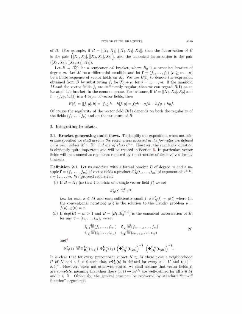
INTEGRATING BRACKETS 4349

of B. (For example, if B = [[X1, X2], [[X3, X4], X5]], then the factorization of B

is the pair(

[X1, X2], [[X3, X4], X5])

, and the canonical factorization is the pair

([X1, X2], [[X1, X2], X3]).

Let B = B(µ)0 be a semicanonical bracket, where B0 is a canonical bracket of

degree m. Let M be a differential manifold and let f = (f1, . . . , fν) (ν ≥ m + µ)be a finite sequence of vector fields on M . We use B(f) to denote the expressionobtained from B by substituting fj for Xj + µ, for j = 1, . . . ,m. If the manifoldM and the vector fields fj are sufficiently regular, then we can regard B(f) as aniterated Lie bracket, in the common sense. For instance, if B = [[X7, X8], X9] andf = (f, g, h, k)) is a 4-tuple of vector fields, then

B(f) = [[f, g], h] = [f, g]h− h[f, g] = fgh− gfh− hfg + hgf.

Of course the regularity of the vector field B(f) depends on both the regularity ofthe fields (f1, . . . , fν) and on the structure of B.

2. Integrating brackets.

2.1. Bracket generating multi-flows. To simplify our exposition, when not oth-erwise specified we shall assume the vector fields involved in the formulas are definedon a open subset M ⊆ R

n and are of class C∞. However, the regularity questionis obviously quite important and will be treated in Section 5. In particular, vectorfields will be assumed as regular as required by the structure of the involved formalbrackets.

Definition 2.1. Let us associate with a formal bracket B of degree m and a m-tuple f = (f1, . . . , fm) of vector fields a product Ψf

B(t1, . . . , tm) of exponentials etifi ,i = 1, . . . ,m. We proceed recursively:

(i) If B = X1 (so that f consists of a single vector field f) we set

Ψf

B(t)def= etf ,

i.e., for each x ∈ M and each sufficiently small t, xΨf

B(t) = y(t) where (inthe conventional notation) y(·) is the solution to the Cauchy problem y =f(y), y(0) = x.

(ii) If deg(B) = m > 1 and B = [B1, B(m1)2 ] is the canonical factorization of B,

for any t = (t1, . . . , tm), we set

f(1)def=(f1, . . . , fm1

) f(2)def=(fm1+1, . . . , fm)

t(1)def=(t1, . . . , tm1) t(2)

def=(tm1+1, . . . , tm)

(9)

and4

Ψf

B(t)def=Ψ

f(1)

B1(t(1)) Ψ

f(2)

B2(tβ)

(

Ψf(1)

B1(t(2))

)−1 (

Ψf(2)

B2(t(2))

)−1

.

It is clear that for every precompact subset K ⊂ M there exist a neighborhoodU of K and a δ > 0 such that xΨf

B(t) is defined for every x ∈ U and t ∈] −δ, δ[m. However, when not otherwise stated, we shall assume that vector fields fiare complete, meaning that their flows (x, t) 7→ xetfi are well-defined for all x ∈ M

and t ∈ R. Obviously, the general case can be recovered by standard “cut-offfunction” arguments.

4350 ERMAL FELEQI AND FRANCO RAMPAZZO

Let us illustrate the above definition of Ψf

B(t) by means of simple examples:

Figure 1. y = xΨ(f,g)[X1,X2]

(t1, t2), z = xΨ(f,g,h)[[X1,X2],X3]

(t1, t2, t3)

1. if B = [X1, X2] and f = (f, g), then

Ψf

B(t1, t2) = et1fet2ge−t1fe−t2g ;

2. if B = [X1, [X2, X3]] and f = (f, g, h), then

Ψf

B(t1, t2, t3) = et1fet2get3he−t2ge−t3he−t1fet3het2ge−t3he−t2g .

3. if B = [X1, X2], [X3, X4]] and f = (f, g, h, k), then

Ψf

B(t1, t2, t3, t4)

= et1fet2ge−t1fe−t2get3het4ke−t3he−t4ket2get1fe−t2ge−t1fet4ket3he−t4ke−t3h .

Observe that the number N(B) of exponential factors of Ψf

B is given recursivelyby N(B) = 1 if deg(B) = 1 and, for m > 1, N(B) = 2(N(B1) + N(B2)), where[B1, B2] is the canonical factorization of B.

2.2. Integrating brackets. The integrating bracket corresponding to B and f willbe defined as a (2m− 2)-parameterized (continuous) vector field on M

x 7→ xB(f)(t1,...,tm1−1,tm1+1,...,tm,s1,...,sm−1),

which, in particular, depends continuously on the parameters

(t1, . . . , tm1−1, tm1+1, . . . , tm, s1, . . . , sm−1) ∈ Rm−1 × R

m−1 ,

and verifies xB(f)(0...,0) = xB(f).To begin with, let us recall the notion of Ad operator:

Definition 2.2. Let U, V ⊆ M be open subsets and let Φ : U → V be a Cr

diffeomorphism (r ≥ 1). If h is a vector field on U , AdΦh is the vector field on U

defined by

x 7→ xAdΦhdef=xΦhΦ−1 ∀x ∈ U

4In [3], [5, 4], akin maps, usually defined for brackets B of the form

[X1, [X2[....[Xm−1, Xm], ], . . . ]

and t of the form (t, . . . , t), are called quasiexponential, almost exponential, or approximate expo-

nential maps.

INTEGRATING BRACKETS 4351

(In the conventional notation, the vector field AdΦh would be denoted by x 7→D(Φ)−1

|Φ(x)(h(Φ(x)))

We remind that the Ad operator is bracket preserving, namely

AdΦ[h1, h2] = [AdΦh1, AdΦh2],

for all vector fields h1, h2.Willing to define integrating brackets of degree greater than 2, we cannot avoid

introducing a few more notation. However, some examples following Definition 2.3should allow one to get an intuitive idea of the bracket’s construction.

If d is any positive integer and r = (r1, . . . , rd) ∈ Rd and α ∈ {1, . . . , d}, let us

use

rα

to denote the (d− 1)-tuple obtained by r by deleting the α-th element. So, forinstance, if r = (r1, r2, r3, r4) one has

r1= (r2, r3, r4) r

2= (r1, r3, r4), r

3= (r1, r2, r4) r

4= (r1, r2, r3)

For α, β ∈ {1, . . . , 2}, α < β, we also let

r{α,β}

denote the (d− 2)-tuple obtained by r by deleting the α-th and β-th elements, sothat, for instance, if r = (r1, r2, r3, r4),

r{2,4}

= (r1, r3).

When d = 1, we set

r1

def= ∅. (10)

Also, if d = 2, we set

r{α,β}

def= ∅. (11)

Let B be an iterated bracket and let B = [B1, B(m1)2 ] be its canonical factor-

ization, with deg(B) = m, deg(B1) = m1, deg(B2) = m2, m = m1 + m2. Letf = (f1, . . . , fm) be an m-tuple of vector fields . We set, as before,

t = (t1, . . . , tm) t(1)def=(t1, . . . , tm1) t(2)

def=(tm1+1, . . . , tm).

Moreover, let

s = (s1, . . . , sm−1) ∈ Rm−1

Definition 2.3 (Integrating bracket). We call integrating bracket (correspond-

ing to the pair (B, f)) the (2m − 2)-parameterized vector field B(f)

(

tm1

,s

)

definedrecursively as follows:

m = 1 If m = 1 (so that B = X1, f = f1), we let

B(f)

(

t1,s

)

= B(f)∅def= f1 . (12)

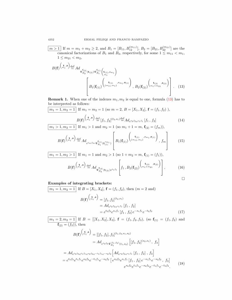
4352 ERMAL FELEQI AND FRANCO RAMPAZZO

m > 1 If m = m1 +m2 ≥ 2, and B1 = [B11, B(m11)12 ], B2 = [B21, B

(m21)22 ] are the

canonical factorizations of B1 and B2, respectively, for some 1 ≤ m11 < m1,1 ≤ m21 < m2,

B(f)

(

tm1

,s

)

def= Ad

Ψf(2)B2

(t(2))Ψf(1)B1

(

t(1)m1

,sm1

)

B1(f(1))

t(1){m11,m1}

,sm1,s(1)

, B2(f(2))

(

t(2)m1+m21

,s(2)

)

. (13)

Remark 1. When one of the indexes m1,m2 is equal to one, formula (13) has tobe interpreted as follows:

m1 = 1,m2 = 1 If m1 = m2 = 1 (so m = 2, B = [X1, X2], f = (f1, f2) ),

B(f)

(

tm1

,s

)

def= [f1, f2]

(t2,s1)def=Adet2f2es1f1 [f1 , f2] (14)

m1 > 1,m2 = 1 If m1 > 1 and m2 = 1 (so m1 + 1 = m, f(2) = (fm)),

B(f)

(

tm1

,s

)

def= Ad

etmfmΨf(1)B1

(tsm1(1)

)

B1(f(1))

t(1){m11,m1}

,sm1,s(1)

, fm

(15)

m1 = 1,m2 > 1 If m1 = 1 and m2 > 1 (so 1 +m2 = m, f(1) = (f1)),

B(f)

(

tm1

,s

)

def= Ad

Ψf(2)B2

(t(2))et1f1

f1 , B2(f(2))

(

t(2)m1+m21

,s(2)

)

, (16)

�

Examples of integrating brackets:

m1 = 1,m2 = 1 If B = [X1, X2], f = (f1, f2), then (m = 2 and)

B(f)

(

tm1

,s

)

= [f1, f2](t2,s1)

= Adet2f2es1f1 [f1 , f2]

= et2f2es1f1 [f1 , f2] e−s1f1e−t2f2 (17)

m1 = 2,m2 = 1 If B = [[X1, X2], X3], f = (f1, f2, f3), (so f(1) = (f1, f2) and

f(2) = (f3)), then

B(f)

(

tm1

,s

)

= [[f1, f2], f3](t1,t3,s1,s2)

= Adet3f3Ψ

(f1,f2)

B1(t1,s2)

[

[f1, f2](s2,s1) , f3

]

= Adet3f3et1f1es2f2e−t1f1e−s2f2

[

Ades2f2es1f1 [f1 , f2] , f3

]

= et3f3et1f1es2f2e−t1f1e−s2f2[

es2f2es1f1 [f1 , f2] e−s1f1e−s2f2 , f3

]

es2f2et1f1e−s2f2e−t1f1e−t3f3 .(18)

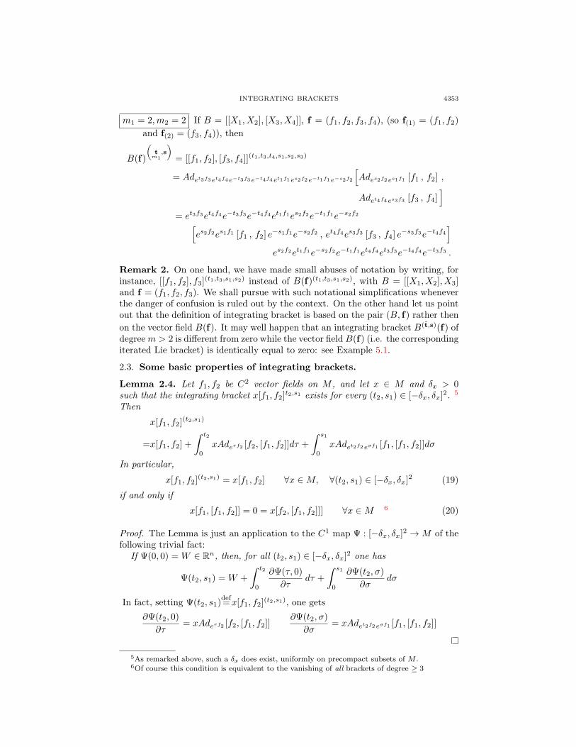
INTEGRATING BRACKETS 4353

m1 = 2,m2 = 2 If B = [[X1, X2], [X3, X4]], f = (f1, f2, f3, f4), (so f(1) = (f1, f2)

and f(2) = (f3, f4)), then

B(f)

(

tm1

,s

)

= [[f1, f2], [f3, f4]](t1,t3,t4,s1,s2,s3)

= Adet3f3et4f4e−t3f3e−t4f4et1f1es2f2e−t1f1e−s2f2

[

Ades2f2es1f1 [f1 , f2] ,

Adet4f4es3f3 [f3 , f4]]

= et3f3et4f4e−t3f3e−t4f4et1f1es2f2e−t1f1e−s2f2

[

es2f2es1f1 [f1 , f2] e−s1f1e−s2f2 , et4f4es3f3 [f3 , f4] e

−s3f3e−t4f4]

es2f2et1f1e−s2f2e−t1f1et4f4et3f3e−t4f4e−t3f3 .

Remark 2. On one hand, we have made small abuses of notation by writing, forinstance, [[f1, f2], f3]

(t1,t3,s1,s2) instead of B(f)(t1,t3,s1,s2), with B = [[X1, X2], X3]and f = (f1, f2, f3). We shall pursue with such notational simplifications wheneverthe danger of confusion is ruled out by the context. On the other hand let us pointout that the definition of integrating bracket is based on the pair (B, f) rather then

on the vector field B(f). It may well happen that an integrating bracket B(t,s)(f) ofdegreem > 2 is different from zero while the vector field B(f) (i.e. the correspondingiterated Lie bracket) is identically equal to zero: see Example 5.1.

2.3. Some basic properties of integrating brackets.

Lemma 2.4. Let f1, f2 be C2 vector fields on M , and let x ∈ M and δx > 0such that the integrating bracket x[f1, f2]

t2,s1 exists for every (t2, s1) ∈ [−δx, δx]2. 5

Then

x[f1, f2](t2,s1)

=x[f1, f2] +

∫ t2

0

xAdeτf2 [f2, [f1, f2]]dτ +

∫ s1

0

xAdet2f2eσf1 [f1, [f1, f2]]dσ

In particular,

x[f1, f2](t2,s1) = x[f1, f2] ∀x ∈ M, ∀(t2, s1) ∈ [−δx, δx]

2 (19)

if and only if

x[f1, [f1, f2]] = 0 = x[f2, [f1, f2]]] ∀x ∈ M 6 (20)

Proof. The Lemma is just an application to the C1 map Ψ : [−δx, δx]2 → M of the

following trivial fact:If Ψ(0, 0) = W ∈ R

n, then, for all (t2, s1) ∈ [−δx, δx]2 one has

Ψ(t2, s1) = W +

∫ t2

0

∂Ψ(τ, 0)

∂τdτ +

∫ s1

0

∂Ψ(t2, σ)

∂σdσ

In fact, setting Ψ(t2, s1)def=x[f1, f2]

(t2,s1), one gets

∂Ψ(t2, 0)

∂τ= xAdeτf2 [f2, [f1, f2]]

∂Ψ(t2, σ)

∂σ= xAdet2f2eσf1 [f1, [f1, f2]]

5As remarked above, such a δx does exist, uniformly on precompact subsets of M .6Of course this condition is equivalent to the vanishing of all brackets of degree ≥ 3

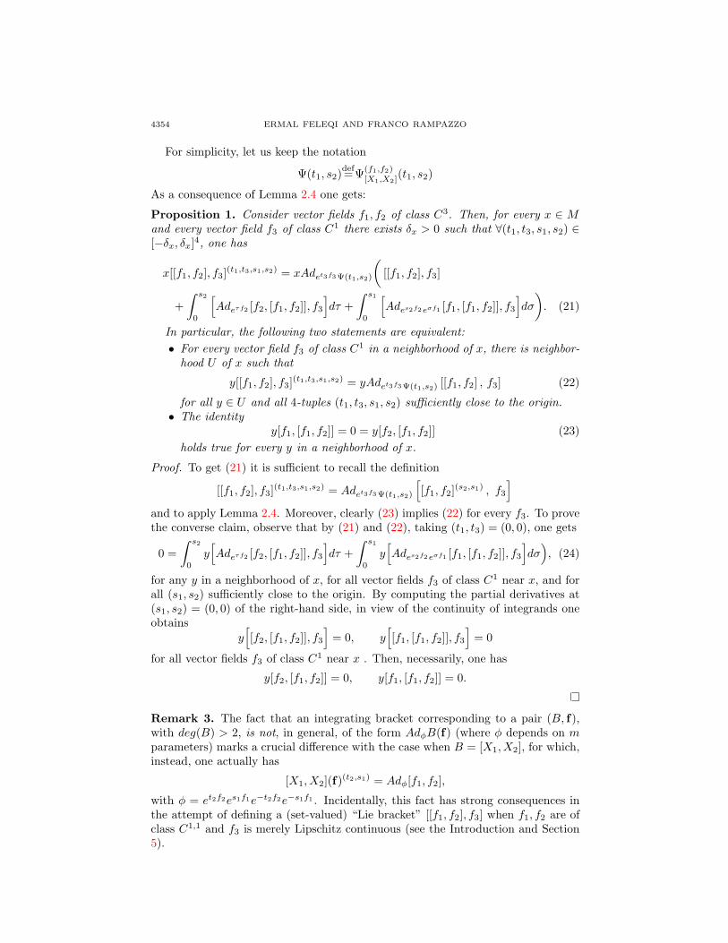
4354 ERMAL FELEQI AND FRANCO RAMPAZZO

For simplicity, let us keep the notation

Ψ(t1, s2)def=Ψ

(f1,f2)[X1,X2]

(t1, s2)

As a consequence of Lemma 2.4 one gets:

Proposition 1. Consider vector fields f1, f2 of class C3. Then, for every x ∈ M

and every vector field f3 of class C1 there exists δx > 0 such that ∀(t1, t3, s1, s2) ∈[−δx, δx]

4, one has

x[[f1, f2], f3](t1,t3,s1,s2) = xAdet3f3Ψ(t1,s2)

(

[[f1, f2], f3]

+

∫ s2

0

[

Adeτf2 [f2, [f1, f2]], f3

]

dτ +

∫ s1

0

[

Ades2f2eσf1 [f1, [f1, f2]], f3

]

dσ

)

. (21)

In particular, the following two statements are equivalent:

• For every vector field f3 of class C1 in a neighborhood of x, there is neighbor-hood U of x such that

y[[f1, f2], f3](t1,t3,s1,s2) = yAdet3f3Ψ(t1,s2) [[f1, f2] , f3] (22)

for all y ∈ U and all 4-tuples (t1, t3, s1, s2) sufficiently close to the origin.• The identity

y[f1, [f1, f2]] = 0 = y[f2, [f1, f2]] (23)

holds true for every y in a neighborhood of x.

Proof. To get (21) it is sufficient to recall the definition

[[f1, f2], f3](t1,t3,s1,s2) = Adet3f3Ψ(t1,s2)

[

[f1, f2](s2,s1) , f3

]

and to apply Lemma 2.4. Moreover, clearly (23) implies (22) for every f3. To provethe converse claim, observe that by (21) and (22), taking (t1, t3) = (0, 0), one gets

0 =

∫ s2

0

y[

Adeτf2 [f2, [f1, f2]], f3

]

dτ +

∫ s1

0

y[

Ades2f2eσf1 [f1, [f1, f2]], f3

]

dσ)

, (24)

for any y in a neighborhood of x, for all vector fields f3 of class C1 near x, and forall (s1, s2) sufficiently close to the origin. By computing the partial derivatives at(s1, s2) = (0, 0) of the right-hand side, in view of the continuity of integrands oneobtains

y[

[f2, [f1, f2]], f3

]

= 0, y[

[f1, [f1, f2]], f3

]

= 0

for all vector fields f3 of class C1 near x . Then, necessarily, one has

y[f2, [f1, f2]] = 0, y[f1, [f1, f2]] = 0.

Remark 3. The fact that an integrating bracket corresponding to a pair (B, f),with deg(B) > 2, is not, in general, of the form AdφB(f) (where φ depends on m

parameters) marks a crucial difference with the case when B = [X1, X2], for which,instead, one actually has

[X1, X2](f)(t2,s1) = Adφ[f1, f2],

with φ = et2f2es1f1e−t2f2e−s1f1 . Incidentally, this fact has strong consequences inthe attempt of defining a (set-valued) “Lie bracket” [[f1, f2], f3] when f1, f2 are ofclass C1,1 and f3 is merely Lipschitz continuous (see the Introduction and Section5).

INTEGRATING BRACKETS 4355

Remark 4. It is trivial to check that condition (23) remains necessary for (22) tohold even if the latter is verified just for n vector fields that are linearly independentat each y ∈ U . Of course, identity (22) may well be true for a particular f3 even if(23) is not verified, as it is immediately apparent by taking f3 ≡ 0, in which case (22)holds with both sides vanishing. However, unless (23) is verified, it is not true thatthe vanishing of [[f1, f2], f3] implies the vanishing of [[f1, f2], f3]

t1,t3,s1,s2 , as shownin Example 5.1 below. As a byproduct of Theorem 3.1 below, this is connectedwith the (almost obvious) fact that in general the condition [[f1, f2], f3] ≡ 0 doesnot imply Ψf

B = IdM .

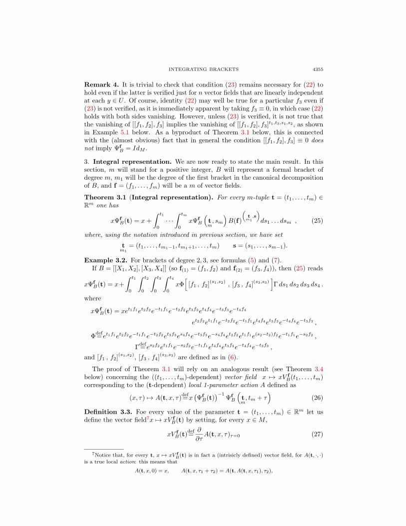
3. Integral representation. We are now ready to state the main result. In thissection, m will stand for a positive integer, B will represent a formal bracket ofdegree m, m1 will be the degree of the first bracket in the canonical decompositionof B, and f = (f1, . . . , fm) will be a m of vector fields.

Theorem 3.1 (Integral representation). For every m-tuple t = (t1, . . . , tm) ∈R

m one has

xΨf

B(t) = x+

∫ t1

0

· · ·

∫ tm

0

xΨf

B

(

tm, sm

)

B(f)

(

tm1

,s

)

ds1 . . . dsm , (25)

where, using the notation introduced in previous section, we have set

tm1

= (t1, . . . , tm1−1, tm1+1, . . . , tm) s = (s1, . . . , sm−1).

Example 3.2. For brackets of degree 2, 3, see formulas (5) and (7).If B = [[X1, X2], [X3, X4]] (so f(1) = (f1, f2) and f(2) = (f3, f4)), then (25) reads

xΨf

B(t) = x+

∫ t1

0

∫ t2

0

∫ t3

0

∫ t4

0

xΦ[

[f1 , f2](s1,s2) , [f3 , f4]

(s3,s3)]

Γ ds1 ds2 ds3 ds4 .

where

xΨf

B(t) = xet1f1et2f2e−t1f1e−t2f2et3f3et4f4e−t3f3e−t4f4

et2f2et1f1e−t2f2e−t1f1et4f4et3f3e−t4f4e−t3f3 ,

Φdef= et1f1et2f2e−t1f1e−t2f2et3f3es4f4e−t3f3e−s4f4et2f2et1f1e(s2−t2)f2e−t1f1e−s2f2 ,

Γdef= es2f2et1f1e−s2f2e−t1f1et4f4et3f3e−t4f4e−t3f3 ,

and [f1 , f2](s1,s2), [f3 , f4]

(s3,s3) are defined as in (6).

The proof of Theorem 3.1 will rely on an analogous result (see Theorem 3.4below) concerning the ((t1, . . . , tm)-dependent) vector field x 7→ xV f

B(t1, . . . , tm)corresponding to the (t-dependent) local 1-parameter action A defined as

(x, τ) 7→ A(t, x, τ)def=x

(

Ψf

B(t))−1

Ψf

B

(

tm, tm + τ

)

(26)

Definition 3.3. Foe every value of the parameter t = (t1, . . . , tm) ∈ Rm let us

define the vector field7x 7→ xV f

B(t) by setting, for every x ∈ M ,

xV f

B(t)def=

∂

∂τA(t, x, τ)τ=0 (27)

7Notice that, for every t, x 7→ xV f

B(t) is in fact a (intrisicly defined) vector field, for A(t, ·, ·)is a true local action: this means that

A(t, x, 0) = x, A(t, x, τ1 + τ2) = A(t, A(t, x, τ1), τ2),

4356 ERMAL FELEQI AND FRANCO RAMPAZZO

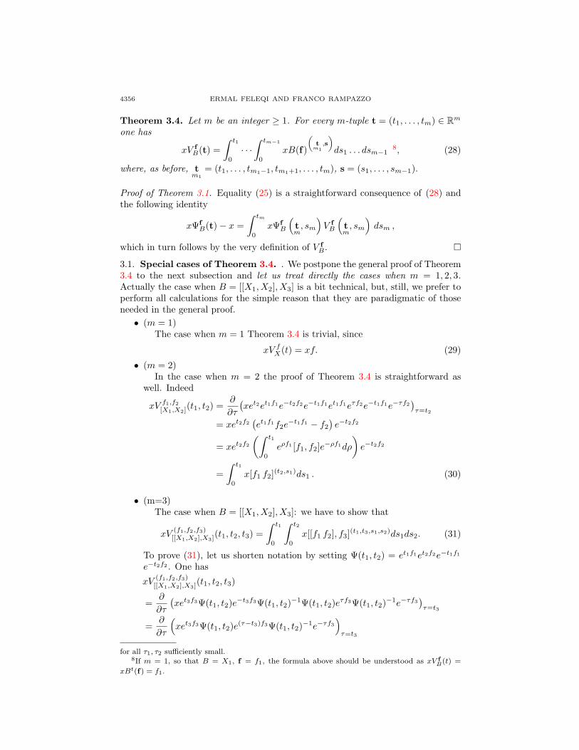
Theorem 3.4. Let m be an integer ≥ 1. For every m-tuple t = (t1, . . . , tm) ∈ Rm

one has

xV f

B(t) =

∫ t1

0

· · ·

∫ tm−1

0

xB(f)

(

tm1

,s

)

ds1 . . . dsm−18, (28)

where, as before, tm1

= (t1, . . . , tm1−1, tm1+1, . . . , tm), s = (s1, . . . , sm−1).

Proof of Theorem 3.1. Equality (25) is a straightforward consequence of (28) andthe following identity

xΨf

B(t)− x =

∫ tm

0

xΨf

B

(

tm, sm

)

V f

B

(

tm, sm

)

dsm ,

which in turn follows by the very definition of V f

B . �

3.1. Special cases of Theorem 3.4. . We postpone the general proof of Theorem3.4 to the next subsection and let us treat directly the cases when m = 1, 2, 3.Actually the case when B = [[X1, X2], X3] is a bit technical, but, still, we prefer toperform all calculations for the simple reason that they are paradigmatic of thoseneeded in the general proof.

• (m = 1)The case when m = 1 Theorem 3.4 is trivial, since

xVfX(t) = xf. (29)

• (m = 2)In the case when m = 2 the proof of Theorem 3.4 is straightforward as

well. Indeed

xVf1,f2[X1,X2]

(t1, t2) =∂

∂τ

(

xet2et1f1e−t2f2e−t1f1et1f1eτf2e−t1f1e−τf2)

τ=t2

= xet2f2(

et1f1f2e−t1f1 − f2

)

e−t2f2

= xet2f2(∫ t1

0

eρf1 [f1, f2]e−ρf1dρ

)

e−t2f2

=

∫ t1

0

x[f1 f2](t2,s1)ds1 . (30)

• (m=3)The case when B = [[X1, X2], X3]: we have to show that

xV(f1,f2,f3)[[X1,X2],X3]

(t1, t2, t3) =

∫ t1

0

∫ t2

0

x[[f1 f2], f3](t1,t3,s1,s2)ds1ds2. (31)

To prove (31), let us shorten notation by setting Ψ(t1, t2) = et1f1et2f2e−t1f1

e−t2f2 . One has

xV(f1,f2,f3)[[X1,X2],X3]

(t1, t2, t3)

=∂

∂τ

(

xet3f3Ψ(t1, t2)e−t3f3Ψ(t1, t2)

−1Ψ(t1, t2)eτf3Ψ(t1, t2)

−1e−τf3)

τ=t3

=∂

∂τ

(

xet3f3Ψ(t1, t2)e(τ−t3)f3Ψ(t1, t2)

−1e−τf3)

τ=t3

for all τ1, τ2 sufficiently small.8If m = 1, so that B = X1, f = f1, the formula above should be understood as xV f

B(t) =

xBt(f) = f1.

INTEGRATING BRACKETS 4357

= xet3f3Ψ(t1, t2)f3Ψ(t1, t2)−1e−t3f3 − xet3f3Ψ(t1, t2)Ψ(t1, t2)

−1f3e−t3f3

= xet3f3Ψ(t1, t2)f3Ψ(t1, t2)−1e−t3f3 − xet3f3f3e

−t3f3

= xet3f3Ψ(t1, t2)f3Ψ(t1, t2)−1e−t3f3 − xet3f3Ψ(t1, 0)f3Ψ(t1, 0)

−1e−t3f3

=

∫ t2

0

∂

∂σ

(

xet3f3Ψ(t1, σ)f3Ψ(t1, σ)−1e−t3f3

)

dσ

=

∫ t2

0

xet3f3∂

∂σ

(

Ψ(t1, σ)f3Ψ(t1, σ)−1)

e−t3f3dσ

(32)

To compute the last integral let us begin by observing that, in view of Defi-nition 3.3, one has

∂

∂σΨ(t1, σ) = Ψ(t1, σ)V

(f1,f2)[X1,X2]

(t1, σ) (33)

Furthermore, let us compute the derivative ∂∂σ

(

Ψ(t1, σ)−1)

, by differentiatingthe relation

Ψ(t1, σ)Ψ(t1, σ)−1 = IdM

with respect to σ. We obtain

0 =∂

∂σ

(

Ψ(t1, σ)Ψ(t1, σ)−1)

=∂

∂σ(Ψ(t1, σ))Ψ(t1, σ)

−1 +Ψ(t1, σ)∂

∂σ

(

Ψ(t1, σ)−1)

= Ψ(t1, σ)V(f1,f2)[X1,X2]

(t1, σ)Ψ(t1, σ)−1 +Ψ(t1, σ)

∂

∂σ

(

Ψ(t1, σ)−1)

,

from which we get

∂

∂σ

(

Ψ(t1, σ)−1)

= −V(f1,f2)[X1,X2]

(t1, σ)Ψ(t1, σ)−1. (34)

Using (33), (34), we can continue the row of equalities in (32), so obtaining

xV(f1,f2,f3)[[X1,X2],X3]

(t1, t2, t3)

=

∫ t2

0

(

xet3f3∂

∂σ(Ψ(t1, σ)) f3Ψ(t1, σ)

−1e−t3f3

+ xet3f3Ψ(t1, σ)f3∂

∂σ

(

Ψ(t1, σ)−1)

e−t3f3)

dσ

=

∫ t2

0

(

xet3f3Ψ(t1, σ)V(f1,f2)[X1,X2]

(t1, σ)f3Ψ(t1, σ)−1e−t3f3

− xet3f3Ψ(t1, σ)f3V(f1,f2)[X1,X2]

(t1, σ)Ψ(t1, σ)−1e−t3f3

)

dσ

=

∫ t2

0

xet3f3Ψ(t1, σ)[

V(f1,f2)[X1,X2]

(t1, σ) , f3

]

Ψ(t1, σ)−1e−t3f3dσ.

Then, using (30), we get

xV(f1,f2,f3)[[X1,X2],X3]

(t1, t2, t3)

=

∫ t2

0

xet3f3Ψ(t1, σ)

[∫ t1

0

[f1 f2](σ,s1)ds1 , f3

]

Ψ(t1, σ)−1e−t3f3dσ

=

∫ t1

0

∫ t2

0

xet3f3Ψ(t1, s2)[

[f1 f2](s2,s1) , f3

]

Ψ(t1, s2)−1e−t3f3ds1ds2

having set σ = s2. Taking into account (18), this is precisely (31).

4358 ERMAL FELEQI AND FRANCO RAMPAZZO

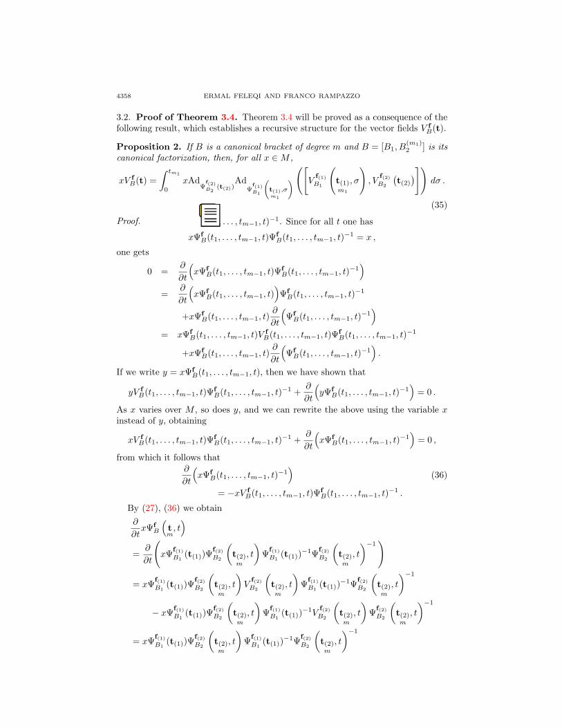
3.2. Proof of Theorem 3.4. Theorem 3.4 will be proved as a consequence of thefollowing result, which establishes a recursive structure for the vector fields V f

B(t).

Proposition 2. If B is a canonical bracket of degree m and B = [B1, B(m1)2 ] is its

canonical factorization, then, for all x ∈ M ,

xV f

B(t) =

∫ tm1

0

xAdΨ

f(2)B2

(t(2))Ad

Ψf(1)B1

(

t(1)m1

,σ

)

([

Vf(1)

B1

(

t(1)m1

, σ

)

, Vf(2)

B2

(

t(2))

])

dσ .

f

B(t1, . . . , tm−1, t)−1. Since for all t one has

xΨf

B(t1, . . . , tm−1, t)Ψf

B(t1, . . . , tm−1, t)−1 = x ,

one gets

0 =∂

∂t

(

xΨf

B(t1, . . . , tm−1, t)Ψf

B(t1, . . . , tm−1, t)−1)

=∂

∂t

(

xΨf

B(t1, . . . , tm−1, t))

Ψf

B(t1, . . . , tm−1, t)−1

+xΨf

B(t1, . . . , tm−1, t)∂

∂t

(

Ψf

B(t1, . . . , tm−1, t)−1)

= xΨf

B(t1, . . . , tm−1, t)Vf

B(t1, . . . , tm−1, t)Ψf

B(t1, . . . , tm−1, t)−1

+xΨf

B(t1, . . . , tm−1, t)∂

∂t

(

Ψf

B(t1, . . . , tm−1, t)−1)

.

If we write y = xΨf

B(t1, . . . , tm−1, t), then we have shown that

yV f

B(t1, . . . , tm−1, t)Ψf

B(t1, . . . , tm−1, t)−1 +

∂

∂t

(

yΨf

B(t1, . . . , tm−1, t)−1)

= 0 .

As x varies over M , so does y, and we can rewrite the above using the variable x

instead of y, obtaining

xV f

B(t1, . . . , tm−1, t)Ψf

B(t1, . . . , tm−1, t)−1 +

∂

∂t

(

xΨf

B(t1, . . . , tm−1, t)−1)

= 0 ,

from which it follows that∂

∂t

(

xΨf

B(t1, . . . , tm−1, t)−1)

(36)

= −xV f

B(t1, . . . , tm−1, t)Ψf

B(t1, . . . , tm−1, t)−1 .

By (27), (36) we obtain

∂

∂txΨf

B

(

tm, t)

=∂

∂t

(

xΨf(1)

B1(t(1))Ψ

f(2)

B2

(

t(2)m

, t

)

Ψf(1)

B1(t(1))

−1Ψf(2)

B2

(

t(2)m

, t

)−1)

= xΨf(1)

B1(t(1))Ψ

f(2)

B2

(

t(2)m

, t

)

Vf(2)

B2

(

t(2)m

, t

)

Ψf(1)

B1(t(1))

−1Ψf(2)

B2

(

t(2)m

, t

)−1

− xΨf(1)

B1(t(1))Ψ

f(2)

B2

(

t(2)m

, t

)

Ψf(1)

B1(t(1))

−1Vf(2)

B2

(

t(2)m

, t

)

Ψf(2)

B2

(

t(2)m

, t

)−1

= xΨf(1)

B1(t(1))Ψ

f(2)

B2

(

t(2)m

, t

)

Ψf(1)

B1(t(1))

−1Ψf(2)

B2

(

t(2)m

, t

)−1

(35)

Proof.

INTEGRATING BRACKETS 4359

(

Ψf(2)

B2

(

t(2)m

, t

)

Ψf(1)

B1(t(1))V

f(2)

B2

(

t(2)m

, t

)

Ψf(1)

B1(t(1))

−1Ψf(2)

B2

(

t(2)m

, t

)−1)

− xΨf(1)

B1(t(1))Ψ

f(2)

B2

(

t(2)m

, t

)

Ψf(1)

B1(t(1))

−1Ψf(2)

B2

(

t(2)m

, t

)−1

(

Ψf(2)

B2

(

t(2)m

, t

)

Vf(2)

B2

(

t(2)m

, t

)

Ψf(2)

B2

(

t(2)m

, t

)−1)

= xΨf

B

(

tm, t)

(

Ψf(2)

B2

(

t(2)m

, t

)

Ψf(1)

B1(t(1))V

f(2)

B2

(

t(2)m

, t

)

Ψf(1)

B1(t(1))

−1

Ψf(2)

B2

(

t(2)m

, t

)−1)

− xΨf

B

(

tm, t)

(

Ψf(2)

B2

(

t(2)m

, t

)

Vf(2)

B2

(

t(2)m

, t

)

Ψf(2)

B2

(

t(2)m

, t

)−1)

,

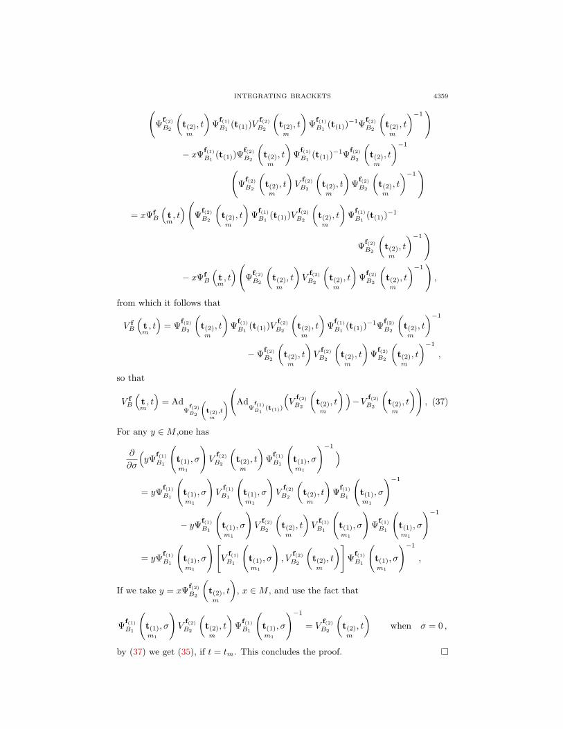
from which it follows that

V f

B

(

tm, t)

= Ψf(2)

B2

(

t(2)m

, t

)

Ψf(1)

B1(t(1))V

f(2)

B2

(

t(2)m

, t

)

Ψf(1)

B1(t(1))

−1Ψf(2)

B2

(

t(2)m

, t

)−1

−Ψf(2)

B2

(

t(2)m

, t

)

Vf(2)

B2

(

t(2)m

, t

)

Ψf(2)

B2

(

t(2)m

, t

)−1

,

so that

V f

B

(

tm, t)

= AdΨ

f(2)B2

(

t(2)m

,t

)

(

AdΨ

f(1)B1

(t(1))

(

Vf(2)

B2

(

t(2)m

, t

)

)

−Vf(2)

B2

(

t(2)m

, t

)

)

, (37)

For any y ∈ M ,one has

∂

∂σ

(

yΨf(1)

B1

(

t(1)m1

, σ

)

Vf(2)

B2

(

t(2)m

, t

)

Ψf(1)

B1

(

t(1)m1

, σ

)−1)

= yΨf(1)

B1

(

t(1)m1

, σ

)

Vf(1)

B1

(

t(1)m1

, σ

)

Vf(2)

B2

(

t(2)m

, t

)

Ψf(1)

B1

(

t(1)m1

, σ

)−1

− yΨf(1)

B1

(

t(1)m1

, σ

)

Vf(2)

B2

(

t(2)m

, t

)

Vf(1)

B1

(

t(1)m1

, σ

)

Ψf(1)

B1

(

t(1)m1

, σ

)−1

= yΨf(1)

B1

(

t(1)m1

, σ

)[

Vf(1)

B1

(

t(1)m1

, σ

)

, Vf(2)

B2

(

t(2)m

, t

)

]

Ψf(1)

B1

(

t(1)m1

, σ

)−1

,

If we take y = xΨf(2)

B2

(

t(2)m

, t

)

, x ∈ M , and use the fact that

Ψf(1)

B1

(

t(1)m1

, σ

)

Vf(2)

B2

(

t(2)m

, t

)

Ψf(1)

B1

(

t(1)m1

, σ

)−1

= Vf(2)

B2

(

t(2)m

, t

)

when σ = 0 ,

by (37) we get (35), if t = tm. This concludes the proof.

4360 ERMAL FELEQI AND FRANCO RAMPAZZO

Proof of Theorem 3.4. Let us proceed by induction on m = deg(B). For m = 1, thethesis simply follows from (29). For m > 1 let us assume the inductive hypothesisfor each of the two subbrackets B1, B2 appearing in the canonical factorization

[B1, B(m1)2 ] of B. So,

xVf(1)

B1

(

t(1)m1

, sm1

)

=

∫ t1

0

· · ·

∫ tm1−1

0

xB1(f(1))

t(1){m11,m1}

,sm1,s(1)

ds1 . . . dsm1−1 ,

(38)

xVf(2)

B2

(

t(2))

=

∫ tm1+1

0

· · ·

∫ tm−1

0

xB2(f(2))

(

t(1)m21

,s(2)

)

dsm1+1 . . . dsm−1 . (39)

If m1 = 1 (resp. if m1 = m−1, i.e., m2 = m−m1 = 1 ), we mean that formula (38)

(resp. (39)) reads xVf(1)

B1(t

sm1

(1) ) = xVf1X1

(s1) = xf1 (resp. xVf(2)

B2(t(2)) = xV

fmX1

(tm) =

xfm).By applying (35) we obtain

xV f

B(t) =

∫ t1

0

· · ·

∫ tm−1

0

xAdΨ

f(2)B2

(t(2))Ad

Ψf(1)B1

(

t(1)m1

,sm1

)

B1(f(1))

t(1){m11,m1}

,sm1,s(1)

, B2(f(2))

(

t(1)m21

,s(2)

)

ds1 . . . dsm−1 .

Since, by Definition 2.3,

xAdΨ

f(2)B2

(t(2))Ad

Ψf(1)B1

(

t(1)m1

,sm1

)

B1(f(1))

t(1){m11,m1}

,sm1,s(1)

, B2(f(2))

(

t(1)m21

,s(2)

)

= xB(f)

(

tm1

,s

)

,

the proof is concluded.

4. “CB” regularity.The main results of this paper remain valid also when vector fields fi fail to

be C∞, provided suitable Cr hypotheses are assumed. To state them, given anm-tuple of vector fields f = (f1, . . . , fm) on M and a canonical bracket B of degreem, we shall define the notion of f of class CB . Roughly speaking, it means thatall components fi, for i = 1, . . . ,m, possess the minimal order of differentiation forwhich B(f) (can be computed everywhere and) is continuous.

As a byproduct of the integral representation provided in Theorem 3.1 we get ver-sions of the asymptotic formulas (and of Chow-Rashevski’s controllability theorem)under quite low regularity hypotheses.

4.1. Number of differentiations. To give a precise meaning to the expression“ f possess the minimal order of differentiation for which B(f) (can be computedeverywhere and) is continuous” we need some formalism concerning the way any

INTEGRATING BRACKETS 4361

bracket B can be regarded as constructed in a recursive way by iterated bracket-ings. In this recursive construction, each subbracket S undergoes a certain numberof bracketings until B is obtained. When we plug in vector fields fj for the inde-terminates Xj , each bracketing involves a differentiation. So we will refer to this“number of bracketings” as “the number of differentiations of S in B,” and use theexpression ∆(S;B) to denote it. Naturally, this will only make sense for bracketsB and subbrackets S such that S only occurs once as a substring of B. For moregeneral brackets, one must define a “subbracket of B” to be not just a string thatoccurs as a substring of B and is a bracket, but as an occurrence of such a string,so that, for example, the two occurrences of X1 in B = [X1, [X1, X2]] count asdifferent subbrackets. Notice that the number of differentiations of X1 in B is 1 forthe first one and 2 for the second one. In order to avoid this extra complication,we will confine ourselves to semicanonical brackets, for which this problem does notarise, because a subbracket S of a semicanonical bracket B can only occur once asa substring of B.

The precise definition of ∆(S;B), B being canonical, and S ∈ Subb(B), is by abackwards recursion on S:

• ∆(B;B)def= 0;

• ∆(S1;B)def= ∆(S2;B)

def= 1 +∆([S1, S2];B) .

It is then easy to prove by induction that

∆(S;B) = nrbr(S;B)− nlbr(S;B) ,

where nrbr(S;B) is the number of right brackets that occur in B to the right of S,and nlbr(S;B) is the number of left brackets that occur in B to the right of S.

For example, if

B = [X3, [[[[X4, X5], X6], X7], [X8, [X9, X10]]]] ,

then ∆([X4, X5];B) = 4.It is easy to see that, if (B1, B2) is the canonical factorization of B, and deg(B1) =

m1, deg(B2) = m2, then

∆(Xj ;B) =

{

∆(Xj ;B1) + 1 if j ∈ {1, . . . ,m1}∆(Xj−m1

;B2) + 1 if j ∈ {m1 + 1, . . . ,m1 +m2} .

The following trivial but important identity then holds:If Xj is a subbracket of S and S is a subbracket B,

∆j(B) = ∆j(S) + ∆(S;B) if Xj and S are subbrackets of B.

Definition 4.1 (Class CB+k). Let m,µ, ν, k be nonnegative integers such thatν ≥ m + µ, m ≥ 1. Given a semicanonical bracket B of degree m such that

B = B(µ)0 , B0 being canonical, and a ν-tuple f = (f1, . . . , fν) of vector fields, we

say that f is of class CB+k if fj is of class C∆j(B)+k for each j ∈ {1+µ, . . . ,m+µ}.We also write f ∈ CB+k to indicate that f is of class CB+k. Finally, we simplifythe notation by just writing CB instead of CB+0.

Remark 5. The above definition can be adapted in a obvious way to the case when

M is just a manifold of class Cℓ for ℓ ≥ 1+k+max{

∆j(B) : j ∈ {1+µ, . . . ,m+µ}}

.

For example, suppose that

B = [[X1, X2], [[X3, X4], X5]] and f = (f1, f2, f3, f4, f5) .

4362 ERMAL FELEQI AND FRANCO RAMPAZZO

Then f ∈ CB if and only if f1, f2, f5 ∈ C2 and f3, f4 ∈ C3.

It is then easy to verify the following result:

Proposition 3. Assume that we are given data B, m, B0, µ, k, ν, and an ν-tuplef = (f1, . . . , fν) as in Definition 4.1. Let (B1, B2) be the factorization of B. Thenf ∈ CB+k if and only if f ∈ CB1+k+1 and f ∈ CB2+k+1.

It then follows, by an easy induction on the subbrackets S of B, that one candefine S(f) for every subbracket S of B as a true vector field, by simply letting

S(f) = [S1(f), S2(f)] if S = [S1, S2] .

The resulting vector field S(f) is of class C∆(S;B)+k as soon as f is of class CB+k.In particular:

• If f ∈ CB+k, then B(f) is a vector field on M of class Ck.

In particular,

• if f ∈ CB then B(f) is a continuous vector field.

4.2. Representation with low regularity, asymptotic formulas, and Chow-

Rashevski’s theorem. One can easily verify that

(

x, tm1

, s

)

7→ B(f)

(

tm1

,s

)

is

well-defined and continuous for any canonical bracket B with canonical factoriza-

tion B = [B1, B(m1)2 ], where 1 ≤ m1 < deg(B), and any f ∈ CB . Moreover,

with obvious reinterpretation of the notation one easily obtains the following lowregularity version of Theorem 3.1:

Theorem 4.2 (Integral representation with CB regularity). Let B be a canonicaliterated bracket of deg(B) = m ≥ 1, and let f be an m-tuple of vector fields on M

of class CB. Then, for every m− tuple t = (t1, . . . , tm) ∈ Rm one has

xΨf

B(t) = x+

∫ t1

0

· · ·

∫ tm

0

xΨf

B

(

tm, sm

)

B(f)

(

tm1

,s

)

ds1 . . . dsm ,

As an almost obvious byproduct we get the following asymptotic formulas underlow regularity assumptions.

Theorem 4.3 (Asymptotic formulas). Let B be a canonical iterated bracket ofdeg(B) = m ≥ 1, and f an m-tuple of vector fields on M . Assume that f ∈ CB.Then we have

xΨf

B(t1, . . . , tm) = x+ t1 · · · tmB(f)(x) + o(t1 · · · tm) (40)

as |(t1, . . . , tm)| → 0.

In turn, as a consequence of the asymptotic formulas above (and via a standardapplication of the open mapping theorem, see e.g. [8]), one gets a low-regularityversion of Chow-Rashevski’s controllability theorem:

Theorem 4.4 (Chow-Rashevski). Let {f1, . . . fr} be a family of (C1) vector fieldson M . Let us consider the driftless control system

x =

r∑

i=1

uifi(x) (41)

with control constraints |ui| ≤ 1 for i = 1, . . . , r. Let x∗ ∈ M , and let B1, . . . , Bℓ

and f1, . . . , fℓ be canonical iterated brackets, and finite collections of the vector fieldsfi, i = 1, . . . r, respectively, such that:

INTEGRATING BRACKETS 4363

• i) for every j = 1, . . . , ℓ, fj ∈ CBj ,• ii)

span{

B1(f1)(x∗), . . . , Bℓ(fℓ)(x∗)}

= Tx∗M (42)

Then the control system (41) is locally controllable from x∗ in small time. Moreprecisely, if d is a Riemannian distance defined on an open set A containing thepoint x∗, and if k is the maximum of the degrees of the iterated Lie brackets Bj,then there exist a neighborhood U ⊂ A of x∗ and a positive constant C such thatfor every x ∈ U one has

T (x) ≤ C(d(x, x∗))1k , (43)

where T (x) denotes the minimum time to reach x over the set of admissible controls,provided that this set contains the piecewise constant controls t → (u1(t), . . . , um(t))such that at each time t only one of the numbers ui(t), i = 1, . . . ,m, is nonzero.

Remark 6. In view of some arguments utilized in [8], the C1-regularity assumptionfor the vector fields fi in Theorem 4.4 may be further weakened: in fact, the onlyneeded regularity hypotheses are those stated at point i). The latter, in turn, allowfor some of the vector fields fi to be just continuous, so that the correspondingflows are set-valued maps. We refer to Subsection 5.2 for other considerations onthe regularity question.

5. Concluding remarks.

5.1. On the “adjoint” structure of integrating brackets. The crucial differ-ence between integrating brackets of degree 2 and brackets of degree greater than2 consists in the fact that while the former are adjoint to the corresponding Lie

brackets, namely [f1, f2](t2,s1)def=Adet2f2es1f1 [f1 , f2] , the latter in general include

intermediate adjoining operations. Indeed this is already true when the degree isequal to three, in that two adjoinings are needed. For instance:

[[f1, f2], f3](t1,t3,s1,s2) = Adet3f3et1f1es2f2e−t1f1e−s2f2

[

Ades2f2es1f1 [f1 , f2] , f3

]

In fact, this would not obstruct the possibility that

[[f1, f2], f3](t1,t3,s1,s2) = Adφ(t1,t3,s1,s2)

[

[f1 , f2] , f3

]

(44)

for some (t1, t3, s1, s2)-dependent diffeomorphism φ. However, let us point out thatif (44) were standing, then, in view of the integral representation provided by The-orem 3.1, the vanishing of the iterated Lie bracket [[f1, f2], f3] would imply that

Ψ(f1,f2,f3)[[X1,X2],X3]

= IdM . Notice incidentally that by Proposition 1, (44) holds true for

any f3, as soon as 0 = [[f1, f2], f2] = [[f1, f2], f1] = 0.

Yet, in general (44) does not hold, so that in general one has Ψ(f1,f2,f3)[[X1,X2],X3]

6= IdM .

This is in fact what we get from the following simple example:

Example 5.1. In M = R2 let us consider the linear vector fields fi(x, y) =

Ai

(

x

y

)

, i = 1, 2, 3, where

A1 =

(

0 01 0

)

, A2 =

(

0 10 0

)

, A3 =

(

1 00 0

)

.

4364 ERMAL FELEQI AND FRANCO RAMPAZZO

Let us show that [[f1, f2], f3] ≡ 0, and nevertheless Ψ(f1,f2,f3)[[X1,X2],X3]

6= IdM . Clearly

[f1, f2], [f1, f2](t2,s1), [[f1, f2], f3], [[f1, f2], f3]

(t1,t3,s1,s2) are also linear (parameter-ized) vector fields: the corresponding matrices are defined, respectively, as 9

[A1, A2]def= A2A1 −A1A2,

[A1, A2](t2,s1) def

= e−t2A2e−s1A1 [A1, A2]es1A1et2A2 ,

[[A1, A2], A3]def= A3A2A1 −A3A1A2 −A2A1A3 +A1A2A3

[[A1, A2], A3](t1,t3,s1,s2) def

= e−t3A3e−t1A1e−s2A2et1A1es2A2

[

[A1, A2](s2,s1), A3

]

e−s2A2e−t1A1es2A2et1A1et3A3 .

One finds

[A1, A2] =

(

1 00 −1

)

, [[A1, A2], A3] =

(

0 00 0

)

,

[A1, A2](t2,s1) =

(

2s1t2 + 1 (2s1t2 + 1)t2 + t2−2s1 −2s1t2 − 1

)

[[A1, A2], A3](t1,t3,s1,s2)

=

(

2s2t1(s2t1 + 1)(−2s1s2 + t1s2 − 1) 2e−t3s22(s1s2 − t1s2 + 1)

−2et3t1(

s22t1

3 − s1(

2s22t1

2 + 2s2t1 + 1))

−2s2(

−s2t12 + s1s2t1 + s1

)

)

.

By definition (or by formula (8)), one gets

(

x

y

)

Ψ(f1,f2,f3)

[[X1,X2],X3](t1, t2, t3) =

(

x

y

)

+

(

t13t2

3e−t3

(

1− et3)

x− t12t2e

−t3(

et3

− 1) (

t12t2

2 + t1t2 + 1)

y

t1t22(

et3

− 1)

(t1t2 − 1)x+ t13t2

3(

et3

− 1)

y

)

for all (x, y) ∈ R2 and t1, t2, t3 ∈ R.

Hence, although [[f1, f2], f3] vanishes (identically), Ψ(f1,f2,f3)[[X1,X2],X3]

(t1, t2, t3) 6= IdM ,

so that (44) cannot hold.

5.2. Nonsmooth vector fields and set-valued Lie brackets. Let us concludewith a theme already mentioned in the Introduction. In [8] the following notion ofset valued Lie bracket [f, g]set has been proposed for locally Lipschitz continuousvector fields f, g: for every x ∈ M , one lets

[f, g]set(x)def= co

{

limj→∞

[f, g](xj) | (xj)j∈N ⊂ DIFF (f) ∩DIFF (g), limj→∞

xj = x

}

,

(45)

9More generally, if B is a canonical bracket of deg(B) = m ≥ 1 with canonical factorization

B = [B1, B(m1)2 ] for 1 ≤ m1 < m, and f = (f1, . . . , fm) an m-tuple of linear vector fields on

some linear space M , then B(f), B(f)

(

tm1

,s

)

are also linear vector fields on M , for all t ∈ Rm,

s ∈ Rm−1. Denoting by A = (A1, . . . , Am) the m-tuple of matrices associated in order to the

components of f with respect to some fixed basis of M , then one can define in an obvious way

matrices B(A), and B(A)

(

tm1

,s

)

in such a way that they be the associated matrices of B(f) and

B(f)

(

tm1

,s

)

with respect to that same basis of M .

INTEGRATING BRACKETS 4365

where co means convex enveloping, and DIFF (f) ⊂ M and DIFF (g) ⊂ M denotethe subsets where f and g, respectively, are differentiable. By Rademacher’s theo-rem, these sets have full measure, so, in particular DIFF (f) ∩DIFF (g) is densein M . The set-valued map x 7→ [f, g]set(x) turns out to be upper semicontinuouswith compact, convex nonempty values. In [8] this bracket has been utilized toprovide a nonsmooth generalization of Chow-Rashevski’s theorem. Successively ithas been also used to prove Frobenius-like and commutativity results for nonsmoothvector fields. Therefore, a natural issue might be a generalization of this notion toformal brackets B of degree m ≥ 3 and vector fields that fail to be of class CB .As mentioned in the introduction, a mere iteration of (45), produces a (set-valued)bracket that is too small for various purposes, notably for asymptotic formulas. Forinstance (see the example in [9]*Section 7) one can find a point x ∈ M and vector

fields f, g with locally Lipschitz derivatives such that, setting hdef= [f, g], the map

t 7→ xΨ(f,g,h)[[X1,X2],X3]

(t, t, t)− x is not o(t3) 10, while

x[[f, g], h]set = x[h, h]set = 0.

Our guess is that a suitable notion of iterated (set-valued) bracket should containmore tangent vectors than those prescribed by definition (45) (namely the limitsof sequences ([[f, g], h](xj))j∈N for (xj)j∈N ⊂ DIFF (h)) with xj → x as j → ∞).More specifically, we think that the nested structure of a formal bracket B, and inparticular, the recursive definition of integrating brackets, suggests a new notion ofset-valued bracket giving rise to asymptotic formulas that might prove useful forobtaining a higher order, non-smooth, Chow-Rashevski type result.

Acknowledgments. We wish to express our deep gratitude to Hector J. Sussmannfor his active help, made in particular of very inspiring ideas, most of which at aquite advanced stage of development. We are also indebted with the anonymousreferees for crucial comments on various aspects of the paper.

REFERENCES

[1] A. A. Agracev and R. V. Gamkrelidze, Exponential representation of flows and a chronological

enumeration, Mat. Sb. (N.S.), 107 (1978), 467–532, 639.[2] A. A. Agracev and R. V. Gamkrelidze, Chronological algebras and nonstationary vector fields,

in Problems in geometry, (Russian), Akad. Nauk SSSR, Vsesoyuz. Inst. Nauchn. i Tekhn.Informatsii, Moscow, 11 (1980), 135–176, 243.

[3] M. Bramanti, L. Brandolini and M. Pedroni, Basic properties of nonsmooth Hormander’svector fields and Poincare’s inequality, Forum Math., 25 (2013), 703–769.

[4] A. Montanari and D. Morbidelli, Nonsmooth Hormander vector fields and their control balls,Trans. Amer. Math. Soc., 364 (2012), 2339–2375.

[5] A. Montanari and D. Morbidelli, Almost exponential maps and integrability results for a classof horizontally regular vector fields, Potential Anal., 38 (2013), 611–633.

[6] A. Montanari and D. Morbidelli, Step-s involutive families of vector fields, their orbits andthe Poincare inequality, J. Math. Pures Appl. (9), 99 (2013), 375–394.

[7] A. Montanari and D. Morbidelli, Generalized Jacobi identities and ball-box theorem for hor-izontally regular vector fields, J. Geom. Anal., 24 (2014), 687–720.

[8] F. Rampazzo and H. J. Sussmann, Set-valued differentials and a nonsmooth version of Chow-Rashevski’s theorem, in Proceedings of the 40th IEEE Conference on Decision and Control,Orlando, FL, December 2001, IEEE Publications, (2001), 2613–2618.

10 If f, g where of class C2 and hence h of class C1, this map would be o(t3), namely

xΨ(f,g,h)[[X1,X2],X3]

(t, t, t)− x = x[[f, g], h] · t3 + o(t3) = o(t3).

4366 ERMAL FELEQI AND FRANCO RAMPAZZO

[9] F. Rampazzo and H. J. Sussmann, Commutators of flow maps of nonsmooth vector fields, J.Differential Equations, 232 (2007), 134–175.

[10] E. T. Sawyer and R. L. Wheeden, Holder continuity of weak solutions to subelliptic equationswith rough coefficients, Mem. Amer. Math. Soc., 180 (2006), x+157pp.

Received May 2014; revised September 2014.

E-mail address: feleqi@math.unipd.itE-mail address: rampazzo@math.unipd.it