Princeton UniversityDepartment of Operations Research

and Financial Engineering

ORF 245Fundamentals of Statistics

Practice Final ExamJanuary ??, 20161:00 – 4:00 pm

Closed book. No computers. Calculators allowed.

You are permitted to use a two-page two-sided cheat sheet.

Return the exam questions and your cheat sheet with your exam booklet.

ADVICE: Spend five minutes now to read the exam from beginning to end. It only takes afew minutes and will give you a good idea of the scope of the exam and that will help youpace yourself through it.

NOTE: I have tried to make the problems “interesting”. Interesting problems are oftenmore difficult than “routine” problems.

(1) (10 pts.) Who’s your mamma?

(2) (5 pts.) Suppose that X , Y , and Z are normal random variables with these meansand variances:

mean varianceX 2 4Y 0 9Z 15 16

Rank the following probabilities (smallest to largest):

P (X ≤ 1), P (Y ≤ −2), P (Z ≤ 12)

(3) (10 pts.) Twin studies: Many characteristics of individuals are determined by ge-netics, but many others are affected by their environment. There is, therefore, muchinterest in comparing identical twins who have been raised apart.

The table below shows the IQs of ten pairs of identical twins who were raisedapart. In each pair, one twin had been raised in a “good” environment and anotherin a “poor” environment.

IQFamily Poor environment Good environment

1 100 1252 65 953 60 1004 125 1205 85 1206 145 1857 55 808 180 2109 60 105

10 135 175The genetic influence on IQ is evident – when one twin has high IQ, the other

often does too. However we can also ask...Do the twins raised in a “good” environment have a different mean IQ from those

raised in a “poor” environment?To answer this question, let X denote the difference in IQ of the “good” envi-

ronment minus the IQ of the twin from the “bad” environment. Test the hypothesisthat the mean µX is zero.

(4) (5 pts.) Recall that a random variable Y has a log-normal distribution if Y = eµ+σX

where X is a standard normal variable (i.e, X has mean zero and variance one).Compute the formula for the pdf of a log-normal distribution.

(5) (10 pts.) In class we discussed confidence intervals for the parameter p of a Bernoullirandom variable. The straight-forward approach relies on the fact that the mean µequals the parameter p and therefore the usual technique of appoximating the vari-ance σ2 by the sample variance s2 gives the standard confidence interval. But, wealso introduced what we called a “better” confidence interval, which is based onthe fact that the variance also has a simple formula relating it to the parameter pand this was used to avoid the approximation of σ2. The same trick can be appliedto other situations in which the underlying distribution has just a single parameterso that both the mean and the variance can be expressed in terms of this parameter.The Poisson distribution is such an example. Let X be a Poisson random variablewith unknown parameter λ. Recall that E(X) = λ and Var(X) = λ. Recall furtherthat, if n is large, then the central limit theorem can be invoked to get the standard

100(1− α)%-confidence interval for λ:

X − zα/2S/√n ≤ λ ≤ X + zα/2S/

√n.

Of course, we could use the fact that Var(X) = λ = E(X) to replace S with√X:

X − zα/2√X/n ≤ λ ≤ X + zα/2

√X/n.

(a) Under the same assumption that n is large, derive a “better” confidence intervalfor λ.

(b) Comment on how similar or different the better interval is relative to the stan-dard interval.

(6) (10 pts.) Suppose you are given a coin and told that it has a 2-to-1 bias. That is, thecoin favors one side coming up that way 66.66% of the time. But you weren’t toldif it favors heads or it favors tails. You must decide. Of course, you could toss thecoin a zillion times and it would be obvious which side it favors. But, to make asimplified exam question, let’s assume you decide to flip the coin n = 7 times andmake a decision based on the outcome of these seven flips.

(a) Formulate a null hypothesis, H0 and an alternative hypothesis, H1.(b) Let X denote the number of times the coin comes up heads in the n = 7

flips. Assuming that Type-I and Type-II errors are equally bad, formulate areasonable H0 rejection region based on the test statistic X .

(c) What is the probability of a Type-I error?(d) What is the probability of a Type-II error?

NOTE: Here is the probability mass function for a Binomial random variable withn = 7 and p = 2/3.

x 0 1 2 3 4 5 6 7p(x) 0.0005 0.0064 0.0384 0.1280 0.2561 0.3073 0.2048 0.0585

(7) (5 pts.) Consider the same coin described in the previous problem. Now supposethat the coin is tossed 100 times and comes up heads 60 times. What’s a 95%confidence interval for the probability p that the coin comes up heads?

(8) (15 pts.) Suppose that X1, X2, . . . , Xn are independent identically distributed withdensity function

f(x) =

{1βe−x/β, x ≥ 0

0, x < 0.

(a) Compute a formula for the mean µ = E(Xi) of the Xi’s.

(b) Compute a formula for the variance σ2 = E((Xi − µ)2) of the Xi’s.(c) What would you suggest as a good estimator for β?(d) Here is a sample of size n = 49:

0.0496 0.1271 0.2060 0.3845 0.1117 0.3066 0.18020.0379 0.0544 0.0340 0.0200 0.0649 2.1014 1.83960.7756 0.4279 1.2035 0.2731 0.3424 0.1953 0.02440.3848 0.3452 0.0482 0.3429 0.6301 0.2157 0.04920.3044 0.1155 0.1481 0.2539 0.2379 0.0164 0.79030.4054 0.2563 0.1693 0.0415 0.2409 0.2632 0.09320.2417 0.0477 0.2427 0.2218 0.2287 0.4685 0.7826

For your convenience, here is the first and second moments of these 49 num-bers:

x = 0.3336 x2 = 0.2812

Find a 95% confidence interval for β.

Hint: In case you have forgotten how to integrate simple exponential functions,here’s a few precomputed integrals you might need:∫ ∞

0

e−xdx = 1,

∫ ∞0

xe−xdx = 1,

∫ ∞0

x2e−xdx = 2,

∫ ∞0

x3e−xdx = 6.

(9) (15 pts.) The stars we observe in the night sky orbit around our Milky Way galaxyonce every few hundred million years. If all the stars circled the Milky Way in lockstep, then we wouldn’t notice any apparent variations in the night sky (ignoring, ofcourse, the daily once-around rotation caused by our own Earth’s rotation). But theydon’t. There’s a certain amount of randomness to the whole process. The stars thatare far from us don’t appear to us to be moving (at least not on human time scales)but some of the nearby stars exhibit rather significant apparent motions relative tothe background stars. The star with the greatest apparent motion is Barnard’s star.Here are two pictures of it that I took through a 10” telescope on my driveway abouttwo years apart:

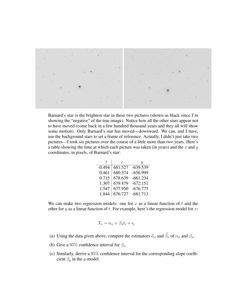
Barnard’s star is the brightest star in these two pictures (shown as black since I’mshowing the “negative” of the true image). Notice how all the other stars appear notto have moved (come back in a few hundred thousand years and they all will showsome motion). Only Barnard’s star has moved—downward. We can, and I have,use the background stars to set a frame of reference. Actually, I didn’t just take twopictures—I took six pictures over the course of a little more than two years. Here’sa table showing the time at which each picture was taken (in years) and the x and ycoordinates, in pixels, of Barnard’s star:

t x y-0.494 681.527 -639.5390.461 680.374 -656.9990.715 678.639 -661.2341.307 679.479 -672.1511.547 677.950 -676.7751.844 676.727 -681.713

We can make two regression models: one for x as a linear function of t and theother for y as a linear function of t. For example, here’s the regression model for x:

Xi = αx + βxti + εi

(a) Using the data given above, compute the estimators α̂x and β̂x of αx and βx.

(b) Give a 95% confidence interval for βx.

(c) Similarly, derive a 95% confidence interval for the corresponding slope coeffi-cient βy in the y-model.

(d) From the focal-length of the telescope and the camera’s pixel size, one canconvert the numbers computed above to standard units of arcseconds/year forthe so-called proper motion of Barnard’s star. The conversion formula for theparticular telescope/camera used is

Proper Motion =√β2x + β2

y × 0.575

Compute the proper motion in arcseconds-per-year.

(Note: Four out of four AI’s surveyed did not know what an arcsecond is. Anarcsecond is a unit of angular measurement. It is a small fraction of a circle.There are 360 degrees in a full circle. There are 60 arcminutes in one degreeand there are 60 arcseconds in one arcminute. So, there are 3600 arcseconds inone degree. As a point of reference, the Moon’s apparent diameter in the skyis about 1/2 degree or, in other words, about 1800 arcseconds.

(e) Explain how you would use bootstrap to produce a 95% confidence interval forthe proper motion. (Note: Pseudo-code in your language of choice is encour-aged here.)

PS. For your computational convenience, we have precomputed some of things youmight need:

t = 0.8967, X = 679.1160, Y = −664.7352t2 = 1.4116, X2 = 461201, Y 2 = 442072

tX = 607.8262, tY = −607.0463, XY = −451410

(10) (15 pts.) This problem is a continuation of the previous one. Here’s a highlyzoomed-in picture showing all six observations overlayed onto one picture and ro-tated so that the apparent proper motion is from left to right:

Note that there seems to be a systematic, perhaps sinusoidal, oscillation. This oscil-lation is no accident. It has a period of exactly one year and it is because the Earthis going around the Sun once a year. Hence, stars that aren’t too far away (such asBarnard’s star) have an apparent annual wobble as viewed against the more distantbackground stars (the background stars also have a wobble, but it is tiny and there-fore unnoticeable). If we can accurately measure the amplitude of this wobble, wecan derive the actual distance to Barnard’s star.

The first step to achieving this goal is to subtract the estimated proper motionfrom the data and then look at the deviation from zero in this adjusted data set. Wehave done that for you. Here are the six deviations (which, for lack of a better letter,we’ll denote by z):

t z-0.4940 -0.14100.4610 0.48330.7150 -0.83751.3070 1.11571.5470 -0.26681.8440 -0.6741

Here’s a plot of these six data points together with the best sinusoidal fit to the data:

time (years)-0.5 0 0.5 1 1.5 2

devia

tion (

pix

els

)

-1

-0.5

0

0.5

1

Parallax

The goal here is to find a formula for the statistical estimator of the amplitude ofthe sine wave. The regression model has a simple form:

Zi = α sin(2πti) + εi.

(a) Derive a least-squares regression formula for an estimator α̂ for the true am-plitude α.

(b) Use the data above to compute α̂.

(c) Explain how you would use bootstrap to produce a 95% confidence interval forα. (Note: Pseudo-code in your language of choice is encouraged here.)

(d) One of the standard units for measuring distance in astronomy is the so-calledparsec (1 parsec = 3.26 lightyears). An object is one parsec away if, by defi-nition, the amplitude of its parallax wobble is one arcsecond. It is 10 parsecsaway if its parallax is 1/10-th of an arcsecond—smaller parallax means greaterdistance. In general, the definition of the distance in parsecs is the reciprocal ofthe parallax angle expressed in arcseconds. Again, the conversion from pixelsto arcseconds requires multipling the number of pixels by 0.575. Hence, theformula for distance in parsecs is:

Parallax Distance = 1/(α× 0.575).

What is your computed distance to Barnard’s star in parsecs?(Comment: In the Star Wars movies, the term parsec is used as a unit of time,not a unit of distance. It’s one of the things George Lucas got wrong.)

Linear Regression Formulas

Here are some useful formulas you probably have on your cheat sheet...Consider the regression model:

Yi = α + βxi + εi

The least-squares regression formulas for the estimators α̂ and β̂ are

β̂ =xY − x Yx2 − x2

α̂ = Y − β̂ xAnd here are formulas for the associated 100(1−α)%-confidence intervals...

α̂− tn−2(α/2)S√n

√x2√

x2 − x2≤ α ≤ α̂+ tn−2(α/2)

S√n

√x2√

x2 − x2

β̂− tn−2(α/2)S√n

1√x2 − x2

≤ β ≤ β̂+ tn−2(α/2)S√n

1√x2 − x2

whereS2 =

1

n− 2

∑i

(Yi − α̂− β̂xi

)2

Appendix B Tables A7

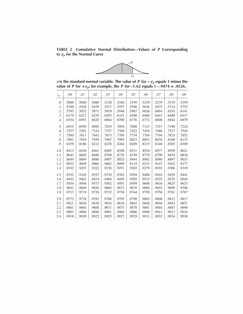
TABLE 2 Cumulative Normal Distribution—Values of P Correspondingto zp for the Normal Curve

zP

P

z is the standard normal variable. The value of P for −zp equals 1 minus thevalue of P for +zp; for example, the P for –1.62 equals 1 – .9474 = .0526.

z p .00 .01 .02 .03 .04 .05 .06 .07 .08 .09

.0 .5000 .5040 .5080 .5120 .5160 .5199 .5239 .5279 .5319 .5359

.1 .5398 .5438 .5478 .5517 .5557 .5596 .5636 .5675 .5714 .5753

.2 .5793 .5832 .5871 .5910 .5948 .5987 .6026 .6064 .6103 .6141

.3 .6179 .6217 .6255 .6293 .6331 .6368 .6406 .6443 .6480 .6517

.4 .6554 .6591 .6628 .6664 .6700 .6736 .6772 .6808 .6844 .6879

.5 .6915 .6950 .6985 .7019 .7054 .7088 .7123 .7157 .7190 .7224

.6 .7257 .7291 .7324 .7357 .7389 .7422 .7454 .7486 .7517 .7549

.7 .7580 .7611 .7642 .7673 .7704 .7734 .7764 .7794 .7823 .7852

.8 .7881 .7910 .7939 .7967 .7995 .8023 .8051 .8078 .8106 .8133

.9 .8159 .8186 .8212 .8238 .8264 .8289 .8315 .8340 .8365 .8389

1.0 .8413 .8438 .8461 .8485 .8508 .8531 .8554 .8577 .8599 .86211.1 .8643 .8665 .8686 .8708 .8729 .8749 .8770 .8790 .8810 .88301.2 .8849 .8869 .8888 .8907 .8925 .8944 .8962 .8980 .8997 .90151.3 .9032 .9049 .9066 .9082 .9099 .9115 .9131 .9147 .9162 .91771.4 .9192 .9207 .9222 .9236 .9251 .9265 .9279 .9292 .9306 .9319

1.5 .9332 .9345 .9357 .9370 .9382 .9394 .9406 .9418 .9429 .94411.6 .9452 .9463 .9474 .9484 .9495 .9505 .9515 .9525 .9535 .95451.7 .9554 .9564 .9573 .9582 .9591 .9599 .9608 .9616 .9625 .96331.8 .9641 .9649 .9656 .9664 .9671 .9678 .9686 .9693 .9699 .97061.9 .9713 .9719 .9726 .9732 .9738 .9744 .9750 .9756 .9761 .9767

2.0 .9772 .9778 .9783 .9788 .9793 .9798 .9803 .9808 .9812 .98172.1 .9821 .9826 .9830 .9834 .9838 .9842 .9846 .9850 .9854 .98572.2 .9861 .9864 .9868 .9871 .9875 .9878 .9881 .9884 .9887 .98902.3 .9893 .9896 .9898 .9901 .9904 .9906 .9909 .9911 .9913 .99162.4 .9918 .9920 .9922 .9925 .9927 .9929 .9931 .9932 .9934 .9936

2.5 .9938 .9940 .9941 .9943 .9945 .9946 .9948 .9949 .9951 .99522.6 .9953 .9955 .9956 .9957 .9959 .9960 .9961 .9962 .9963 .99642.7 .9965 .9966 .9967 .9968 .9969 .9970 .9971 .9972 .9973 .99742.8 .9974 .9975 .9976 .9977 .9977 .9978 .9979 .9979 .9980 .99812.9 .9981 .9982 .9982 .9983 .9984 .9984 .9985 .9985 .9986 .9986

3.0 .9987 .9987 .9987 .9988 .9988 .9989 .9989 .9989 .9990 .99903.1 .9990 .9991 .9991 .9991 .9992 .9992 .9992 .9992 .9993 .99933.2 .9993 .9993 .9994 .9994 .9994 .9994 .9994 .9995 .9995 .99953.3 .9995 .9995 .9995 .9996 .9996 .9996 .9996 .9996 .9996 .99973.4 .9997 .9997 .9997 .9997 .9997 .9997 .9997 .9997 .9997 .9998

A8 Appendix B Tables

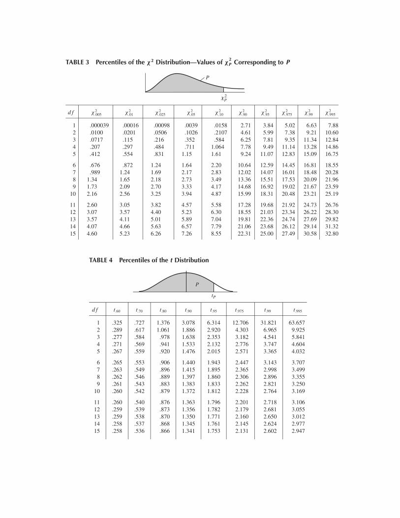
TABLE 3 Percentiles of the χ2 Distribution—Values of χ2P Corresponding to P

P2

P

d f χ2.005 χ2

.01 χ2.025 χ2

.05 χ2.10 χ2

.90 χ2.95 χ2

.975 χ2.99 χ2

.995

1 .000039 .00016 .00098 .0039 .0158 2.71 3.84 5.02 6.63 7.882 .0100 .0201 .0506 .1026 .2107 4.61 5.99 7.38 9.21 10.603 .0717 .115 .216 .352 .584 6.25 7.81 9.35 11.34 12.844 .207 .297 .484 .711 1.064 7.78 9.49 11.14 13.28 14.865 .412 .554 .831 1.15 1.61 9.24 11.07 12.83 15.09 16.75

6 .676 .872 1.24 1.64 2.20 10.64 12.59 14.45 16.81 18.557 .989 1.24 1.69 2.17 2.83 12.02 14.07 16.01 18.48 20.288 1.34 1.65 2.18 2.73 3.49 13.36 15.51 17.53 20.09 21.969 1.73 2.09 2.70 3.33 4.17 14.68 16.92 19.02 21.67 23.59

10 2.16 2.56 3.25 3.94 4.87 15.99 18.31 20.48 23.21 25.19

11 2.60 3.05 3.82 4.57 5.58 17.28 19.68 21.92 24.73 26.7612 3.07 3.57 4.40 5.23 6.30 18.55 21.03 23.34 26.22 28.3013 3.57 4.11 5.01 5.89 7.04 19.81 22.36 24.74 27.69 29.8214 4.07 4.66 5.63 6.57 7.79 21.06 23.68 26.12 29.14 31.3215 4.60 5.23 6.26 7.26 8.55 22.31 25.00 27.49 30.58 32.80

16 5.14 5.81 6.91 7.96 9.31 23.54 26.30 28.85 32.00 34.2718 6.26 7.01 8.23 9.39 10.86 25.99 28.87 31.53 34.81 37.1620 7.43 8.26 9.59 10.85 12.44 28.41 31.41 34.17 37.57 40.0024 9.89 10.86 12.40 13.85 15.66 33.20 36.42 39.36 42.98 45.5630 13.79 14.95 16.79 18.49 20.60 40.26 43.77 46.98 50.89 53.67

40 20.71 22.16 24.43 26.51 29.05 51.81 55.76 59.34 63.69 66.7760 35.53 37.48 40.48 43.19 46.46 74.40 79.08 83.30 88.38 91.95

120 83.85 86.92 91.58 95.70 100.62 140.23 146.57 152.21 158.95 163.64

For large degrees of freedom,

χ2P = 1

2 (zP + √2v − 1)2 approximately,

where v = degrees of freedom and zP is given in Table 2.

Appendix B Tables A9

TABLE 4 Percentiles of the t Distribution

tP

P

d f t.60 t.70 t.80 t.90 t.95 t.975 t.99 t.995

1 .325 .727 1.376 3.078 6.314 12.706 31.821 63.6572 .289 .617 1.061 1.886 2.920 4.303 6.965 9.9253 .277 .584 .978 1.638 2.353 3.182 4.541 5.8414 .271 .569 .941 1.533 2.132 2.776 3.747 4.6045 .267 .559 .920 1.476 2.015 2.571 3.365 4.032

6 .265 .553 .906 1.440 1.943 2.447 3.143 3.7077 .263 .549 .896 1.415 1.895 2.365 2.998 3.4998 .262 .546 .889 1.397 1.860 2.306 2.896 3.3559 .261 .543 .883 1.383 1.833 2.262 2.821 3.250

10 .260 .542 .879 1.372 1.812 2.228 2.764 3.169

11 .260 .540 .876 1.363 1.796 2.201 2.718 3.10612 .259 .539 .873 1.356 1.782 2.179 2.681 3.05513 .259 .538 .870 1.350 1.771 2.160 2.650 3.01214 .258 .537 .868 1.345 1.761 2.145 2.624 2.97715 .258 .536 .866 1.341 1.753 2.131 2.602 2.947

16 .258 .535 .865 1.337 1.746 2.120 2.583 2.92117 .257 .534 .863 1.333 1.740 2.110 2.567 2.89818 .257 .534 .862 1.330 1.734 2.101 2.552 2.87819 .257 .533 .861 1.328 1.729 2.093 2.539 2.86120 .257 .533 .860 1.325 1.725 2.086 2.528 2.845

21 .257 .532 .859 1.323 1.721 2.080 2.518 2.83122 .256 .532 .858 1.321 1.717 2.074 2.508 2.81923 .256 .532 .858 1.319 1.714 2.069 2.500 2.80724 .256 .531 .857 1.318 1.711 2.064 2.492 2.79725 .256 .531 .856 1.316 1.708 2.060 2.485 2.787

26 .256 .531 .856 1.315 1.706 2.056 2.479 2.77927 .256 .531 .855 1.314 1.703 2.052 2.473 2.77128 .256 .530 .855 1.313 1.701 2.048 2.467 2.76329 .256 .530 .854 1.311 1.699 2.045 2.462 2.75630 .256 .530 .854 1.310 1.697 2.042 2.457 2.750

40 .255 .529 .851 1.303 1.684 2.021 2.423 2.70460 .254 .527 .848 1.296 1.671 2.000 2.390 2.660

120 .254 .526 .845 1.289 1.658 1.980 2.358 2.617∞ .253 .524 .842 1.282 1.645 1.960 2.326 2.576