organizing the global value chain - … · organizing the global value chain 2129 in this paper, we...
TRANSCRIPT

http://www.econometricsociety.org/
Econometrica, Vol. 81, No. 6 (November, 2013), 2127–2204
ORGANIZING THE GLOBAL VALUE CHAIN
POL ANTRÀSHarvard University, Cambridge, MA 02138, U.S.A.
DAVIN CHORNational University of Singapore, Singapore 117570, Singapore
The copyright to this Article is held by the Econometric Society. It may be downloaded,printed and reproduced only for educational or research purposes, including use in coursepacks. No downloading or copying may be done for any commercial purpose without theexplicit permission of the Econometric Society. For such commercial purposes contactthe Office of the Econometric Society (contact information may be found at the websitehttp://www.econometricsociety.org or in the back cover of Econometrica). This statement mustbe included on all copies of this Article that are made available electronically or in any otherformat.
Econometrica, Vol. 81, No. 6 (November, 2013), 2127–2204
ORGANIZING THE GLOBAL VALUE CHAIN
BY POL ANTRÀS AND DAVIN CHOR1
We develop a property-rights model of the firm in which production entails a contin-uum of uniquely sequenced stages. In each stage, a final-good producer contracts witha distinct supplier for the procurement of a customized stage-specific component. Ourmodel yields a sharp characterization for the optimal allocation of ownership rightsalong the value chain. We show that the incentive to integrate suppliers varies system-atically with the relative position (upstream versus downstream) at which the supplierenters the production line. Furthermore, the nature of the relationship between inte-gration and “downstreamness” depends crucially on the elasticity of demand faced bythe final-good producer. Our model readily accommodates various sources of asymme-try across final-good producers and across suppliers within a production line, and weshow how it can be taken to the data with international trade statistics. Combining datafrom the U.S. Census Bureau’s Related Party Trade database and estimates of U.S. im-port demand elasticities from Broda and Weinstein (2006), we find empirical evidencebroadly supportive of our key predictions. In the process, we develop two novel mea-sures of the average position of an industry in the value chain, which we construct usingU.S. Input–Output Tables.
KEYWORDS: Property-rights theory, contractual frictions, sequential production,downstreamness, intrafirm trade.
1. INTRODUCTION
MOST PRODUCTION PROCESSES are sequential in nature. At a broad level, theprocess of manufacturing cannot commence until the efforts of R&D centersin the development or improvement of products have proven to be successful,while the sales and distribution of manufactured goods cannot be carried outuntil their production has taken place. Even within manufacturing processes,there is often a natural sequencing of stages. First, raw materials are convertedinto basic components, which are next combined with other components toproduce more complicated inputs, before themselves being assembled into fi-nal goods. This process very much resembles Henry Ford’s original Model T
1We thank the editor and three anonymous referees for their helpful comments and sugges-tions. We are also grateful to Arnaud Costinot, Don Davis, Ron Findlay, Elhanan Helpman,Kala Krishna, Marc Melitz, Esteban Rossi-Hansberg, Daniel Trefler, Jonathan Vogel, and DavidWeinstein, as well as audiences at Berkeley Haas, Chicago, Columbia, Harvard, Northeastern,Notre Dame, NYU Stern, Princeton, Stanford, UCLA, UNH, Wisconsin, Kiel, Munich, Tübin-gen, Bonn, City University of Hong Kong, HKUST, Nanyang Technological University, NationalUniversity of Singapore, Singapore Management University, the Econometric Society WorldCongress (Shanghai), the Society for the Advancement of Economic Theory Conference (Singa-pore), the Asia Pacific Trade Seminars (Honolulu), the Australasian Trade Workshop (UNSW),and the NBER Summer Institute. We thank Nathan Nunn for making available his data. RuiqingCao, Mira Frick, Gurmeet Singh Ghumann, Frank Schilbach, and Zhicheng Song provided ex-cellent research assistance. Chor acknowledges the hospitality of the International EconomicsSection at Princeton, as well as research funding provided by a Sing Lun Fellowship at SingaporeManagement University. All errors are our own.
© 2013 The Econometric Society DOI: 10.3982/ECTA10813
2128 P. ANTRÀS AND D. CHOR
production assembly line, but recent revolutionary advances in informationand communication technology, coupled with a gradual reduction in naturaland man-made trade barriers, now allow such value chains to be “sliced up”into geographically separated steps.
The implications of such sequential production for the workings of open-economy general equilibrium models have been widely explored in the litera-ture. Several papers, most notably Findlay (1978), Dixit and Grossman (1982),Sanyal (1983), Kremer (1993), Kohler (2004), and Costinot, Vogel, and Wang(2013), have emphasized that the pattern of specialization along the valuechain has implications for the world income distribution and for how shocksspread across countries. Others, including Yi (2003), Harms, Lorz, and Urban(2012), and Baldwin and Venables (2013), have unveiled interesting nonlin-earities in the response of trade flows to changes in trade frictions in models ofproduction where value is added sequentially along locations around the globe.
The focus of our paper is different. Our aim is to understand how the se-quentiality of production shapes the contractual relationships between final-good producers and their various suppliers, and how the allocation of controlrights along the value chain can be designed in a way that elicits (constrained)optimal effort on the part of suppliers. An obvious premise of our work is that,although absent from most general equilibrium models, contractual frictionsare relevant for the efficiency with which production is carried out, and also forthe way in which production processes are organized across borders. We findthis to be a natural premise particularly in international trade environments,in which determining which country’s laws are applicable to particular contrac-tual disputes is often difficult. The detrimental effects of imperfect contractenforcement on international trade flows are particularly acute in transactionsinvolving intermediate inputs, as these tend to be associated with longer lagsbetween the time an order is placed (and the contract is signed) and the timethe goods or services are delivered (and the contract is executed). Such transac-tions, moreover, often entail significant relationship-specific investments andother sources of lock-in on the part of both buyers and suppliers.2 The rele-vance of contracting frictions for the organization of production also now restson solid empirical underpinnings.3
2Suppliers often customize their output to the needs of particular buyers and would find ithard to sell those goods to alternative buyers, should the intended buyer decide not to abide bythe terms of the contract. Similarly, buyers often undertake significant investments whose returncan be severely diminished by incompatibilities, production line delays, or quality debasementsassociated with suppliers not going through with their contractual obligations.
3A recent literature (see, for instance, Nunn (2007) and Levchenko (2007)) has convincinglydocumented that contracting institutions are an important determinant of international special-ization. Another branch of the trade literature, to which our paper will contribute, has also shownthat the ownership decisions of multinational firms exhibit various patterns that are consistentwith Grossman and Hart’s (1986) incomplete-contracting, property-rights theory of firm bound-aries (see, among others, Antràs (2003), Nunn and Trefler (2008, 2013), and Bernard, Jensen,Redding, and Schott (2010)).

ORGANIZING THE GLOBAL VALUE CHAIN 2129
In this paper, we develop a property-rights model of firm boundaries thatpermits an analysis of the optimal allocation of ownership rights in a settingwhere production is sequential in nature and contracts are incomplete. Ourmodel builds on Acemoglu, Antràs, and Helpman (2007). Production of finalgoods entails a large number (formally, a continuum) of production stages.Each stage is performed by a different supplier, who needs to undertake arelationship-specific investment in order to produce components that will becompatible with those produced by other suppliers in the value chain. The ser-vices of these components are combined according to a constant-elasticity-of-substitution (CES) aggregator by a final-good producer that faces an isoelasticdemand curve. Contracts between final-good producers and their suppliers areincomplete in the sense that contracts contingent on whether components arecompatible or not cannot be enforced by third parties.
The key innovation relative to Acemoglu, Antràs, and Helpman (2007)—andrelative to the previous property-rights models of multinational firm bound-aries in Antràs (2003, 2005) and Antràs and Helpman (2004, 2008)—is thatwe introduce a natural (or technological) ordering of production stages, sothat production at a stage cannot commence until the inputs or componentsfrom all upstream stages have been delivered. Absent a binding initial (ex ante)agreement, the firm and its suppliers are left to sequentially bargain over howthe surplus associated with a particular stage is to be divided between the firmand the particular stage supplier. As in Grossman and Hart (1986), in thisincomplete-contracting environment, owning a supplier is a source of powerfor the firm because the residual rights of control associated with ownershipallow the firm to take actions (or make threats) that enhance their bargain-ing power vis-à-vis the supplier. However, the optimal allocation of ownershiprights does not always entail all production stages being integrated because, byreducing the bargaining power of suppliers, integration reduces the incentivesof suppliers to invest in the relationship.4
We begin in Section 2 by developing a benchmark model of firm behav-ior that isolates the role of the degree of “downstreamness” of a supplierin shaping organizational decisions. A key feature of our analysis is that therelationship-specific investments made by suppliers in upstream stages affectthe incentives to invest of suppliers in downstream stages. The nature of thisdependence is shaped, in turn, by whether suppliers’ investments are sequentialcomplements or sequential substitutes, according to whether higher investmentlevels by prior suppliers increase or decrease the value of the marginal productof a particular supplier’s investment. Even though, from a strict technologicalpoint of view (i.e., in light of the CES aggregator of inputs), inputs are always
4Zhang and Zhang (2008, 2011) introduced sequential elements in a standard Grossman andHart (1986) model, but focused on one-supplier environments in which either the firm or thesupplier has a first-mover advantage. Other papers that have studied optimal incentive provisionin sequential production processes include Winter (2006) and Kim and Shin (2012).
2130 P. ANTRÀS AND D. CHOR
complements, suppliers’ investments can still prove to be sequential substituteswhen the price elasticity of demand faced by the final-good producer is suffi-ciently low, since in such cases, the value of the marginal product of supplierinvestments falls particularly quickly along the value chain. Whether inputs aresequential complements or sequential substitutes turns out to be determinedonly by whether the elasticity of final-good demand is (respectively) higher orlower than the elasticity of substitution across the services provided by the dif-ferent suppliers’ investments.
The central result of our model is that the optimal pattern of ownershipalong the value chain depends critically on whether production stages are se-quential complements or substitutes. When the demand faced by the final-good producer is sufficiently elastic, then there exists a unique cutoff produc-tion stage such that all stages prior to this cutoff are outsourced, while all stages(if any) after that threshold are integrated. Intuitively, when inputs are se-quential complements, the firm chooses to forgo control rights over upstreamsuppliers in order to incentivize their investment effort, since this generatespositive spillovers on the investment decisions to be made by downstream sup-pliers. When demand is, instead, sufficiently inelastic, the converse predictionholds: it is optimal to integrate relatively upstream stages, and if outsourcing isobserved along the value chain, it necessarily occurs relatively downstream.
In Section 3, we show that these results are robust to alternative contract-ing and bargaining assumptions, and stem mainly from the sequential natureof production rather than the sequential nature of bargaining. Furthermore,we show that our framework can easily accommodate a hybrid of sequentialand modular production processes (or “snakes” and “spiders” in the terminol-ogy of Baldwin and Venables (2013)) as well as several other features whichhave been built into the recent models of global sourcing cited earlier. Theseinclude (headquarter) investments by the final-good producer, productivityheterogeneity across final-good producers, productivity and cost differencesacross suppliers within a production chain, and partial contractibility. Theseextensions prove useful in guiding our empirical analysis.
In Sections 4 and 5, we develop an empirical test of the main predictionsof our framework. The nature and scope of our test are shaped in significantways by data availability. Although our model does not explicitly distinguishbetween domestic and offshore sourcing decisions of firms, data on domes-tic sourcing decisions are not publicly available. We therefore follow the bulkof the recent empirical literature on multinational firm boundaries in usingU.S. Census data on intrafirm trade to measure the relative prevalence of ver-tical integration in particular industries.5 More specifically, we correlate the
5See, for example, Nunn and Trefler (2008, 2013), Bernard et al. (2010), and Díez (2010).Antràs (2013) contains a comprehensive survey of empirical papers using other data sets, includ-ing several firm-level studies, that have similarly used the intrafirm import share to capture thepropensity toward integration relative to outsourcing.

ORGANIZING THE GLOBAL VALUE CHAIN 2131
share of U.S. intrafirm imports in total U.S. imports reported during the period2000–2010 with the average degree of “downstreamness” of that industry, andwe study whether this dependence is qualitatively different for the sequentialcomplements versus sequential substitutes cases. We propose two measuresof downstreamness, both of which are constructed from the 2002 U.S. Input–Output Tables. Our first measure is the ratio of the aggregate direct use to theaggregate total use (DUse_TUse) of a particular industry i’s goods, where thedirect use for a pair of industries (i� j) is the value of goods from industry i di-rectly used by firms in industry j to produce goods for final use, while the totaluse for (i� j) is the value of goods from industry i used either directly or indi-rectly (via purchases from upstream industries) in producing industry j’s outputfor final use. A high value of DUse_TUse thus suggests that most of the con-tribution of input i tends to occur at relatively downstream production stagesthat are close to (one stage removed from) final demand. Our second measureof downstreamness (DownMeasure) is a weighted index of the average positionin the value chain at which an industry’s output is used (i.e., as final consump-tion, as direct inputs to other industries, as direct inputs to industries servingas direct inputs to other industries, and so on), with the weights being given bythe ratio of the use of that industry’s output in that position relative to the totaloutput of that industry. Although constructing such a measure would appearto require computing an infinite power series, we show that DownMeasure canbe succinctly expressed as a simple function of the square of the Leontief in-verse matrix. As discussed in Antràs, Chor, Fally, and Hillberry (2012), there isa close connection between DownMeasure and the measure of distance to finaldemand derived independently by Fally (2012).
Our empirical tests also call on us to distinguish between the cases of sequen-tial complements and substitutes identified in the theory. For that purpose,we use the U.S. import demand elasticities estimated by Broda and Weinstein(2006) and data on U.S. Input–Output Tables to compute a weighted averageof the demand elasticity faced by the buyers of goods from each particularindustry i. The idea is that, for sufficiently high (respectively, low) values ofthis average demand elasticity, we can be relatively confident that input sub-stitutability is lower (respectively, higher) than the demand elasticity. Ideally,one would have used direct estimates of cross-input substitutability (and howthey compare to demand elasticities) to distinguish between the two theoret-ical scenarios, but, unfortunately, these estimates are not readily available inthe literature.
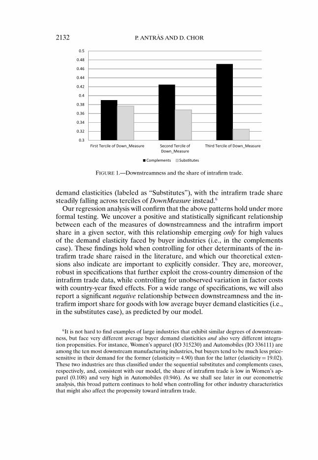
Figure 1 provides a preliminary illustration of our key empirical findings,which lend broad support for the theoretical implications of our model. As isapparent from the dark bins, for the subset of industries with above-medianaverage buyer demand elasticities (labeled as “Complements”), the averageU.S. intrafirm import share (for the year 2005) rises as we move from the lowesttercile of DownMeasure to the highest. In the light bins, this pattern is exactlyreversed when considering those industries facing below-median average buyer
2132 P. ANTRÀS AND D. CHOR
FIGURE 1.—Downstreamness and the share of intrafirm trade.
demand elasticities (labeled as “Substitutes”), with the intrafirm trade sharesteadily falling across terciles of DownMeasure instead.6
Our regression analysis will confirm that the above patterns hold under moreformal testing. We uncover a positive and statistically significant relationshipbetween each of the measures of downstreamness and the intrafirm importshare in a given sector, with this relationship emerging only for high valuesof the demand elasticity faced by buyer industries (i.e., in the complementscase). These findings hold when controlling for other determinants of the in-trafirm trade share raised in the literature, and which our theoretical exten-sions also indicate are important to explicitly consider. They are, moreover,robust in specifications that further exploit the cross-country dimension of theintrafirm trade data, while controlling for unobserved variation in factor costswith country-year fixed effects. For a wide range of specifications, we will alsoreport a significant negative relationship between downstreamness and the in-trafirm import share for goods with low average buyer demand elasticities (i.e.,in the substitutes case), as predicted by our model.
6It is not hard to find examples of large industries that exhibit similar degrees of downstream-ness, but face very different average buyer demand elasticities and also very different integra-tion propensities. For instance, Women’s apparel (IO 315230) and Automobiles (IO 336111) areamong the ten most downstream manufacturing industries, but buyers tend to be much less price-sensitive in their demand for the former (elasticity = 4.90) than for the latter (elasticity = 19.02).These two industries are thus classified under the sequential substitutes and complements cases,respectively, and, consistent with our model, the share of intrafirm trade is low in Women’s ap-parel (0.108) and very high in Automobiles (0.946). As we shall see later in our econometricanalysis, this broad pattern continues to hold when controlling for other industry characteristicsthat might also affect the propensity toward intrafirm trade.

ORGANIZING THE GLOBAL VALUE CHAIN 2133
The remainder of this paper is organized as follows. In Section 2, we developour benchmark model of sequential production with incomplete contractingand study the optimal ownership structure along the value chain. In Section 3,we develop a few theoretical extensions and discuss how we attempt to take themodel to the data. We describe our data sources and empirical specification inSection 4, and present the results in Section 5. Section 6 offers some concludingremarks. All the proofs in the paper are relegated to the Appendix (and theSupplemental Material (Antràs and Chor (2013))).
2. A MODEL OF SEQUENTIAL PRODUCTION WITH INCOMPLETE CONTRACTS
We begin by developing a benchmark model of firm behavior along the linesof Acemoglu, Antràs, and Helpman (2007), but extended to incorporate a de-terministic sequencing of production stages. The model is stylized so as toemphasize the new insights that emerge from considering the sequentiality ofproduction. We will later incorporate more realistic features and embed theframework in industry equilibrium to guide the empirical analysis.
2.1. Benchmark Model
2.1.1. Sequential Production
We consider the organizational problem of a firm producing a final good.Production requires the completion of a measure one of production stages. Weindex these stages by j ∈ [0�1], with a larger j corresponding to stages furtherdownstream (closer to the final end product), and we let x(j) be the services ofcompatible intermediate inputs that the supplier of stage j delivers to the firm.The quality-adjusted volume of final-good production is then given by
q= θ(∫ 1
0x(j)αI(j)dj
)1/α
�(1)
where θ is a productivity parameter, α ∈ (0�1) is a parameter that captures the(symmetric) degree of substitutability among the stage inputs, and I(j) is anindicator function such that:
I(j)=⎧⎨⎩
1� if input j is producedafter all inputs j′ < j have been produced�
0� otherwise.
We normalize x(j) = 0 if an incompatible input is delivered at stage j. Al-though production requires completion of all stages, note that α > 0 ensuresthat output remains positive even when some stages might be completed withincompatible inputs. In words, although all stages are essential from an engi-neering point of view, we allow some substitution in how the characteristics of
2134 P. ANTRÀS AND D. CHOR
these inputs shape the quality-adjusted volume of final output. For example,producing a car requires four wheels, two headlights, one steering wheel, andso on, but the value of this car for consumers will typically depend on the ser-vices obtained from these different components, with a high quality in certainparts partly making up for inferior quality in others.
Our production function in (1) resembles a conventional CES function witha continuum of inputs, but the indicator function I(j) makes the productiontechnology inherently sequential in that downstream stages are useless unlessthe inputs from upstream stages have been delivered. In fact, the technologyin (1) can be expressed in differential form by applying Leibniz’s rule as
q′(m)= 1αθαx(m)αq(m)1−αI(m)�
where q(m) = θ(∫ m
0 x(j)αI(j)dj)1/α. Thus, the marginal increase in output
brought about by the supplier at stage m is given by a simple Cobb–Douglasfunction of this supplier’s (compatible) input production and the quality-adjusted volume of production generated up to that stage (which can be viewedas an intermediate input to the stage-m production process).
2.1.2. Input Production
There is a large number of profit-maximizing suppliers who can engage ei-ther in intermediate input production or in an alternative activity that deliversan outside option normalized to 0. We assume that each intermediate inputmust be produced by a different supplier with whom the firm needs to con-tract. Each supplier must undertake a relationship-specific investment in orderto produce a compatible input. For simplicity, we assume that the input is fullycustomized to the final-good producer, so the value of this input for alterna-tive buyers is equal to 0. To highlight the asymmetries that will arise solely fromthe sequencing of production, we assume that production stages are otherwisesymmetric: the marginal cost of investment is common for all suppliers andequal to c, and in all stages j ∈ [0�1], one unit of investment generates oneunit of services of the stage-j compatible input when combined with the inputsfrom upstream suppliers. (We will relax these symmetry assumptions later inSection 3.) Incompatible inputs can be produced by all agents (including thefirm) at a negligible marginal cost, but they add no value to final-good produc-tion apart from allowing the continuation of the production process.
2.1.3. Preferences
The final good under study is differentiated in the eyes of consumers. Thegood belongs to an industry in which firms produce a continuum of goods andconsumers have preferences that feature a constant elasticity of substitution

ORGANIZING THE GLOBAL VALUE CHAIN 2135
across these varieties. More specifically, denoting by ϕ(ω) the quality of a va-riety and by q̃(ω) its consumption in physical units, the sub-utility accruingfrom this industry is given by
U =(∫
ω∈Ω
(ϕ(ω)q̃(ω)
)ρdω
)1/ρ
with ρ ∈ (0�1)�(2)
where Ω denotes the set of varieties. Note that these preferences feature di-minishing marginal utility with respect to not only the quantity but also thequality of the goods consumed. As a result, in our previous car example, fur-ther quality improvements on a high-end car would not add as much satis-faction to consumers as they would in a low-end car. As is well known, whenmaximizing (2) subject to the budget constraint
∫ω∈Ω p(ω)q̃(ω)dω=E, where
E denotes expenditure, consumer demand for a particular variety features aconstant price elasticity equal to 1/(1 − ρ). Furthermore, the implied revenuefunction of a firm that sells variety ω is concave in quality-adjusted outputq(ω)≡ ϕ(ω)q̃(ω) with a constant elasticity ρ. Combining this feature with theproduction technology in (1), the revenue obtained by the final-good produc-ing firm under study can be written as
r =A1−ρθρ(∫ 1
0x(j)αI(j)dj
)ρ/α�(3)
where A> 0 is an industry-wide demand shifter that the firm treats as exoge-nous.
2.1.4. Complete Contracts
Before discussing in detail our contracting assumptions, it is instructive toconsider first the case of complete contracts in which the firm has full controlover all investments and thus over input services at all stages. In such a case, thefirm makes a contract offer [x(j)� s(j)] for every input j ∈ [0�1], under which asupplier is obliged to supply x(j) of compatible input services as stipulated inthe contract in exchange for the payment s(j). It is clear that the firm will havean incentive to follow the natural sequencing of production, so that I(j) = 1for all j, and the optimal contract simply solves the following maximizationprogram:
max{x(j)�s(j)}j∈[0�1]
A1−ρθρ(∫ 1
0x(j)α dj
)ρ/α−∫ 1
0s(j)dj
s.t. s(j)− cx(j)≥ 0
Solving this problem delivers a common investment level x = (ρA1−ρθρ/c)1/(1−ρ) for all intermediate inputs and associated firm profits equal to π =(1 − ρ)A(ρθ/c)ρ/(1−ρ), while leaving suppliers with a net payoff equal to theiroutside option of zero (i.e., s = cx).

2136 P. ANTRÀS AND D. CHOR
2.1.5. Incomplete Contracts
For the above contracts to be enforceable, it is important that a court of lawbe able to verify the precise value of the input services provided by the suppli-ers of the different stages. In practice, however, a court of law will generallynot be able to verify whether inputs are compatible or not, and whether theservices provided by compatible inputs are in accordance with what was stipu-lated in a written contract. Notice also that the firm might be reluctant to signbinding contracts that are contingent on the quantity of inputs produced butnot on whether inputs are compatible, because suppliers might then have everyincentive to produce incompatible inputs at a negligible cost and still demandpayment. One could envision that contracts contingent on total revenues couldprovide investment incentives for suppliers, but in our setting, with a contin-uum of suppliers, these types of contracts have no value, as they would elicitzero investment levels. For these reasons, it is natural to study situations inwhich the terms of exchange between the firm and the suppliers are not dis-ciplined by an ex ante enforceable contract. In fact, the initial contract is as-sumed to specify only whether suppliers are vertically integrated into the firmor remain independent. In Section 3.4, we will briefly discuss the case of par-tial contractibility, in which some aspects of production (such as the quantityproduced) are contractible ex ante.
Given the lack of a binding contract, a familiar holdup problem emerges.The actual payment to a particular supplier (say, for stage m) is negotiated bi-laterally only after the stage-m input has been produced and the firm has hada chance to inspect it. For the time being, we treat this negotiation indepen-dently from the bilateral negotiations that take place at other stages (thoughwe will revisit this assumption in Section 3.1). Because the intermediate inputis assumed compatible only with the firm’s output, the supplier’s outside optionat the bargaining stage is 0. Hence, the quasi-rents over which the firm and thesupplier negotiate are given by the incremental contribution to total revenuegenerated by supplier m at that stage. To compute this incremental contribu-tion, note that the firm has no incentive to approach suppliers in an orderdifferent from that dictated by the technological sequencing of production andthat it can always unilaterally complete a production stage by producing an in-compatible input.7 As a result, we have I(j)= 1 for all j < m, and the value offinal-good production secured up to stage m is given by
r(m)=A1−ρθρ[∫ m
0x(j)α dj
]ρ/α(4)
7The assumption that the firm is able to complete any production stage with incompatible in-puts may seem strong, but it can be relaxed by considering environments with partial contractibil-ity, as in Grossman and Helpman (2005). For instance, if a fraction of the suppliers’ investmentsis verifiable and contractible, then the firm could use a formal contract to ensure the provision ofa minimum amount of compatible input services from the supplier, and the production processwould never stall.

ORGANIZING THE GLOBAL VALUE CHAIN 2137
Applying Leibniz’s integral rule to this expression, we then have that the incre-mental contribution of supplier m is given by
r ′(m)= ∂r(m)
∂m= ρ
α
(A1−ρθρ
)α/ρr(m)(ρ−α)/ρx(m)α(5)
Following the property-rights theory of firm boundaries, we let the effectivebargaining power of the firm vis-à-vis a particular supplier depend on whetherthe firm owns this supplier or not. As in Grossman and Hart (1986), we assumethat ownership of suppliers is a source of power, in the sense that the firm isable to extract a higher share of surplus from integrated suppliers than fromnonintegrated suppliers. Intuitively, when contracts are incomplete, the factthat an integrating party controls the physical assets used in production willallow that party to dictate a use of these assets that tilts the division of surplusin its favor. To keep our model as tractable as possible, we will not specify indetail the nature of these ex post negotiations and will simply assume that thefirm will obtain a share βV of the incremental contribution in equation (5)when the supplier is integrated, but only a share βO < βV of that surplus whenthe supplier is a stand-alone entity.
We now summarize the timeline of the game played by the firm and thecontinuum of suppliers:8
• The firm posts contracts for suppliers for each stage j ∈ [0�1] of the pro-duction process. The contract stipulates the organizational form—integrationwithin the boundaries of the firm or arm’s-length outsourcing—under whichthe potential supplier will operate.
• Suppliers apply for each contract and the firm chooses one supplier foreach production stage.
• Production takes place sequentially. At the beginning of each stagem, thesupplier is handed the final good completed up to that stage. After observingthe value of this unfinished product (i.e., r(m) in (4)), the supplier chooses aninput level, x(m). At the end of the stage, the firm and supplierm bargain overthe addition to total revenue that supplier m has contributed at stage m (i.e.,r ′(m) in (5)), and the firm pays the supplier.
• Output of the final good is realized once the final stage is completed. Thetotal revenue, A1−ρqρ, from the sale of the final good is collected by the firm.
Before describing the equilibrium of this game, it is worth pausing to brieflydiscuss our assumptions regarding the sequential nature of contracting andpayments. Notice, in particular, that we have assumed that the firm and thesupplier bargain only at stagem, that these agents are not allowed to exchange
8Although we focus throughout on a version of the model with a continuum of productionstages, our equilibrium corresponds to the limit ε → 0 of a discrete game in which M sup-pliers each control a measurable range ε = 1/M of the continuum of intermediate inputs. SeeAcemoglu, Antràs, and Helpman (2007) for an analogous derivation.
2138 P. ANTRÀS AND D. CHOR
lump-sum transfers, and that the terms of exchange are not renegotiated at alater stage and do not reflect the outcome of subsequent negotiations betweenthe firm and other suppliers. Although some of these assumptions could bemotivated in richer frameworks appealing to the existence of incomplete in-formation and limited commitment frictions (as in Hart and Moore (1994) orThomas and Worrall (1994)), these assumptions may admittedly seem special.For these reasons, in Section 3.1, we will explore the robustness of our resultsto alternative contracting and bargaining assumptions.
2.2. Equilibrium Firm Behavior
2.2.1. Supplier Investment in Stage m
We now characterize the subgame perfect equilibrium of the game describedabove. We start by solving for the investment level of a particular stage-m sup-plier, taking as given the value of production up to that stage and the chosenorganizational mode for that stage. Denote by β(m) the share of the incremen-tal contribution r ′(m) that accrues to the firm in its bargaining with supplierm.Our previous discussion implies that
β(m)={βO� if the firm outsources stage m�βV > βO� if the firm integrates stage m
The stage-m supplier obtains the remaining share 1 − β(m) ∈ [0�1] of r ′(m),and thus chooses an investment level x(m) to solve
maxx(m)
πS(m)= (1 −β(m))ρα
(A1−ρθρ
)α/ρr(m)(ρ−α)/ρx(m)α − cx(m)�(6)
which delivers
x(m)=[(
1 −β(m))ρ(A1−ρθρ)α/ρ
c
]1/(1−α)r(m)(ρ−α)/(ρ(1−α))(7)
The investment made by supplier m is naturally increasing in the demandlevel, A, the productivity θ of the firm, and the supplier’s bargaining share,1 − β(m), while it decreases in the investment marginal cost, c. Hence, otherthings equal, an outsourcing relationship (corresponding to a lower β(m)) pro-motes higher investments on the part of supplier m. The effect of the value ofproduction secured up to stagem (and thus of all investment decisions in priorstages, {x(j)}mj=0) is more subtle. If ρ > α, then investment choices are sequen-tial complements in the sense that higher investment levels by prior suppliers,as summarized in r(m), increase the marginal return of supplier m’s own in-vestment. Conversely, if ρ < α, investment choices are sequential substitutesbecause high values of upstream investments reduce the marginal return to

ORGANIZING THE GLOBAL VALUE CHAIN 2139
investing in x(m). Throughout the paper, we shall thus refer to ρ > α as thecomplements case and to ρ < α as the substitutes case.
Since α ∈ (0�1), it is straightforward to verify that, from a purely technolog-ical point of view, supplier investments are always (weakly) complementary.More precisely, in light of equation (1), ∂q/∂x(m) is necessarily nondecreas-ing in the investment decisions of other suppliers m′ �=m. Why is x(m) thennegatively affected by prior investments when ρ < α? The reason is that, whenρ < 1, the firm faces a downward-sloping demand curve for its product, andthus prior upstream investments also affect x(m) on account of the inducedmovements along the demand curve. When ρ is very small, the firm’s rev-enue function is highly concave in quality-adjusted output, and thus marginalrevenue falls at a relatively fast rate along the value chain. In other words,in industries where firms enjoy significant market power, large upstream in-vestment levels can significantly reduce the value of undertaking downstreaminvestments, thus effectively turning supplier investments (in quality-adjustedterms) into sequential substitutes. Equation (7) illustrates that this effect willdominate the standard physical output complementarity effect whenever theelasticity of demand faced by the firm is lower than the elasticity of substitu-tion across inputs, namely when ρ < α.
2.2.2. Suppliers’ Investments Along the Value Chain
Equation (7) characterizes supplier m’s investment level as a function ofr(m), the value of production up to stage m. We next solve for r(m) as a func-tion of the primitives of the model and obtain the equilibrium investment lev-els of all suppliers along the value chain. To achieve this, first plug equation (7)into equation (5) to obtain
r ′(m)= ρ
α
((1 −β(m))ρθ
c
)α/(1−α)Aα(1−ρ)/(ρ(1−α))r(m)(ρ−α)/(ρ(1−α))(8)
This constitutes a differential equation in r(m), which is easily solved by notingthat it is separable in r(m) and β(m). Using the initial condition r(0)= 0, wehave
r(m)=A
(1 − ρ1 − α
)ρ(1−α)/(α(1−ρ))(ρθ
c
)ρ/(1−ρ)(9)
×[∫ m
0
(1 −β(j))α/(1−α)
dj
]ρ(1−α)/(α(1−ρ))
Equation (9) illustrates how the value of production secured up to stage mdepends on all upstream organizational decisions, namely the β(j) for j < m.

2140 P. ANTRÀS AND D. CHOR
Finally, plugging this solution into equation (7) yields
x(m)=A
(1 − ρ1 − α
)(ρ−α)/(α(1−ρ))(ρ
c
)1/(1−ρ)θρ/(1−ρ)(1 −β(m))1/(1−α)
(10)
×[∫ m
0
(1 −β(j))α/(1−α)
dj
](ρ−α)/(α(1−ρ))
From this expression, it is clear that the outsourcing of stage m (i.e., choos-ing β(m) = βO < βV ) enhances investment by that stage’s supplier, while thedependence of x(m) on the prior (upstream) organizational choices of thefirm crucially depends on whether investment decisions are sequential com-plements (ρ > α) or sequential substitutes (ρ < α). In choosing its optimalorganizational structure, the firm will weigh these considerations together withthe fact that outsourcing of any stage is associated with capturing a lower shareof surplus and thus extracting less quasi-rents from suppliers. We next turn tostudy this optimal organizational structure formally.
2.2.3. Optimal Organizational Structure
The firm seeks to maximize the amount of revenue it obtains when the goodis sold net of all payments made to suppliers along the value chain. The firm’sprofits can thus be evaluated as πF = ∫ 1
0 β(j)r′(j)dj, which, after substituting
in the expressions from (8) and (9), is given by
πF =Aρ
α
(1 − ρ1 − α
)(ρ−α)/(α(1−ρ))(ρθ
c
)ρ/(1−ρ) ∫ 1
0β(j)(1 −β(j))α/(1−α)
(11)
×[∫ j
0
(1 −β(k))α/(1−α)
dk
](ρ−α)/(α(1−ρ))dj
It is, in turn, easily verified that the payoff πS(m) obtained by suppliers (seeequation (6)) is always positive, so their participation constraint can be ig-nored. The firm’s decision problem is then
max{β(j)}j∈[0�1]
πF
s.t. β(j) ∈ {βV �βO}�
namely, to choose the organizational mode for each stage j so as to maximizeits profits πF as given in (11).
To determine if integration or outsourcing is optimal at a given stage m,it proves useful to follow the approach in Antràs and Helpman (2004, 2008)

ORGANIZING THE GLOBAL VALUE CHAIN 2141
and consider first the relaxed problem in which the firm could freely choosethe function β(m) from the whole set of piecewise continuously differentiablereal-valued functions rather than from those that only take on values in the set{βV �βO}. Defining
v(j)≡∫ j
0
(1 −β(k))α/(1−α)
dk�(12)
we can write this problem as that of choosing the real-valued function v thatmaximizes the functional:
πF(v)= κ∫ 1
0
(1 − v′(j)(1−α)/α)v′(j)v(j)(ρ−α)/(α(1−ρ)) dj�(13)
where κ ≡ Aρ
α( 1−ρ
1−α)(ρ−α)/(α(1−ρ))( ρ
c)ρ/(1−ρ) is a positive constant.9 The profit-
maximizing function v must then satisfy the Euler–Lagrange condition, which,in light of (13), is given by
v(ρ−α)/(α(1−ρ))(v′)(1−α)/α−1[v′′ + ρ− α
1 − ρ(v′)2
v
]= 0�(14)
provided that v′ is at least piecewise differentiable. In the Appendix, we showthat the profit-maximizing function v must set the term in the square bracketsin (14) to 0. Imposing the initial condition v(0)= 0 and the transversality con-dition v′(1)(1−α)/α = α, and using (12), we can then conclude that the optimaldivision of surplus at stage m, which we denote by β∗(m), is simply given by
β∗(m)= 1 − αm(α−ρ)/α(15)
Proposition 1 then follows.
PROPOSITION 1: The (unconstrained) optimal bargaining share β∗(m) is anincreasing function of m in the complements case (ρ > α), while it is a decreasingfunction of m in the substitutes case (ρ < α).
Before describing the implications of this proposition, it is worth pausing tobriefly discuss two technical issues on which we further elaborate in the Sup-plemental Material (Antràs and Chor (2013)). First, equation (15) was derivedappealing to the Euler–Lagrange condition, which is a necessary condition foroptimality. In the Supplemental Material, we also solve the Hamilton–Jacobi–
9We thank an anonymous referee for suggesting this approach.

2142 P. ANTRÀS AND D. CHOR
Bellman equation associated with our problem and use it to demonstrate thatour optimality condition is also sufficient for a maximum. Second, we have notconstrained the optimal bargaining share β∗(m) to be nonnegative, consistentwith the notion that the firm might find it optimal to compensate certain suppli-ers with a payoff that exceeds their marginal contribution. In the SupplementalMaterial, we show how imposing β∗(m)≥ 0 affects the solution for the optimalbargaining share. Crucially, however, the statement in Proposition 1 remainsvalid except for the fact that, in this constrained case, β∗(m) is only weaklyincreasing in m when ρ > α.
The key implication of Proposition 1 is that the relative size of the param-eters ρ and α will govern whether the incentive for the firm to retain a largersurplus share increases or decreases along the value chain. Intuitively, whenρ is high relative to α, investments are sequential complements, and integrat-ing early stages of production is particularly costly because this reduces theincentives to invest not only of these early suppliers but also of all suppli-ers downstream. Furthermore, although integration allows the firm to capturesome rents, the incremental surplus over which the firm and the supplier nego-tiate is particularly small in these early stages of production. Conversely, whenρ is small relative to α, investments are sequential substitutes, and outsourc-ing is particularly costly in upstream stages because high investments early inthe value chain lead to reduced incentives to invest for downstream suppli-ers, whereas the firm would capture a disproportionate amount of surplus byintegrating these early stages.
Another way to convey this intuition is by comparing the supplier’s in-vestment levels in the complete versus incomplete contracting environments.As we have seen earlier, in the former case, the firm would choose quality-contingent contracts to elicit a common value of input services for all suppli-ers in the value chain. Instead, with incomplete contracting, if the bargainingweight β(m) was common for all stages, investment levels would be increasingalong the value chain for ρ > α and decreasing along the value chain for ρ < α(see equation (7)). The optimal choice of β(m) in (15) can thus be understoodas a second-best instrument that attenuates the distortions arising from incom-plete contracting, by rebalancing investment levels toward those that would bechosen in the absence of contracting frictions. In the complements case, thisinvolves eliciting more supplier investment in the early stages through out-sourcing, and (possibly) integrating the most downstream suppliers to dampenthe relative overinvestment in these latter stages; an analogous logic applies inthe substitutes case.
Evaluating the function β∗(m) in (15) at its extremes, we obtain thatlimm→0β
∗(m) = −∞ when ρ > α and β∗(0) = 1 when ρ < α, while β∗(1) =1 − α regardless of the relative magnitude of α and ρ. This implies that whenthe firm is constrained to choose β(m) from the pair of values βV and βO ,the decision of whether or not to integrate the most upstream stages depends

ORGANIZING THE GLOBAL VALUE CHAIN 2143
FIGURE 2.—Profit-maximizing division of surplus for stage m.
solely on the relative size of ρ and α. In the complements case, the firm wouldselect the minimum possible value of β(m) at m = 0, which corresponds tochoosing outsourcing in this initial stage and, by continuity, in a measurable setof the most upstream stages. Conversely, in the substitutes case, the firm nec-essarily chooses to integrate these initial stages. As for the most downstreamstages, the decision is less clear-cut. In both cases, if βV < 1 − α= β∗(1), thenit is clear that last stage will be integrated, while it will necessarily be out-sourced if βO > 1 − α. When βV > 1 − α > βO , whether stages in the immedi-ate neighborhood of m= 1 are integrated or not depends on other parameterrestrictions (see the Appendix). Figure 2 depicts the function β∗(m) when-ever βV > 1 − α > βO , in which case there is the potential for integrated andoutsourced stages to coexist along the value chain in both the sequential com-plements and substitutes cases.
Our discussion so far has focused on the optimal organizational mode forstages at both ends of the value chain. In the Appendix, we show that the setof stages under a common organizational form (integration or outsourcing) isnecessarily a connected interval in [0�1], thus implying the following.
PROPOSITION 2: In the complements case (ρ > α), there exists a unique m∗C ∈
(0�1], such that: (i) all production stages m ∈ [0�m∗C) are outsourced; and (ii) all
stages m ∈ [m∗C�1] are integrated within firm boundaries. In the substitutes case
(ρ < α), there exists a unique m∗S ∈ (0�1], such that: (i) all production stages m ∈
[0�m∗S) are integrated within firm boundaries; and (ii) all stages m ∈ [m∗
S�1] areoutsourced.
Given that β(m) takes on at most two values along the value chain, one canin fact derive a closed-form solution for the cutoff stages, m∗
C and m∗S , in terms

2144 P. ANTRÀS AND D. CHOR
of the parameters βO , βV , α, and ρ (see Appendix for details):
m∗C = min
⎧⎪⎪⎪⎪⎨⎪⎪⎪⎪⎩
⎡⎢⎢⎢⎣1 +
(1 −βO1 −βV
)α/(1−α)(16)
×
⎡⎢⎢⎢⎣⎛⎜⎜⎜⎝
1 − βO
βV
1 −(
1 −βO1 −βV
)−α/(1−α)
⎞⎟⎟⎟⎠α(1−ρ)/(ρ−α)
− 1
⎤⎥⎥⎥⎦⎤⎥⎥⎥⎦
−1
�1
⎫⎪⎪⎪⎪⎬⎪⎪⎪⎪⎭
and
m∗S = min
⎧⎪⎪⎪⎪⎨⎪⎪⎪⎪⎩
⎡⎢⎢⎢⎢⎣1 +
(1 −βV1 −βO
)α/(1−α)(17)
×
⎡⎢⎢⎢⎢⎣⎛⎜⎜⎜⎝(
1 −βV1 −βO
)−α/(1−α)− 1
βV
βO− 1
⎞⎟⎟⎟⎠α(1−ρ)/(α−ρ)
− 1
⎤⎥⎥⎥⎥⎦
⎤⎥⎥⎥⎥⎦
−1
�1
⎫⎪⎪⎪⎪⎬⎪⎪⎪⎪⎭�
where, remember, βO < βV .10 With these expressions, we can then establishthe following.
PROPOSITION 3: Whenever integration and outsourcing coexist along the valuechain (i.e., m∗
C ∈ (0�1) when ρ > α, or m∗S ∈ (0�1) when ρ < α), a decrease in ρ
will necessarily expand the range of stages that are vertically integrated.
The negative effect of ρ on integration is explained by the fact that, when thefirm has relatively high market power (low ρ), it will tend to place a relativelyhigh weight on the rent-extraction motive for integration and will thus be lessconcerned with the investment inefficiencies caused by such integration.
10Using (16) and (17), it is straightforward to derive the parameter restrictions that character-ize when the cutoff lies strictly in the interior of (0�1). In the complements case, m∗
C ∈ (0�1) ifβV (1−βV )α/(1−α) > βO(1−βO)α/(1−α), whilem∗
C = 1 otherwise. In the substitutes case,m∗S ∈ (0�1)
if βV (1 −βV )α/(1−α) < βO(1 −βO)α/(1−α), while m∗S = 1 otherwise (see the Appendix).

ORGANIZING THE GLOBAL VALUE CHAIN 2145
3. EXTENSIONS AND EMPIRICAL IMPLEMENTATION
Our Benchmark Model is stylized along several directions and omits manyfactors that have been shown to be important for the organizational decisionsof firms in the global economy. In this section, we develop a few extensions thathelp us gauge the robustness of our results and also allow us to connect ourBenchmark Model to the global sourcing framework in Antràs and Helpman(2004, 2008). These extensions will also serve to justify the regression specifi-cation and several control variables that we will adopt later in our empiricalanalysis. For simplicity, we develop these extensions one at a time, althoughthey could readily be incorporated in a unified framework.
3.1. Alternative Contracting Assumptions
3.1.1. Ex ante Transfers
We begin by exploring the robustness of our results to alternative contractingassumptions. (To conserve space, we focus on outlining the main results, andrelegate most mathematical details to the Supplemental Material.) We firstconsider the implications of allowing for ex ante transfers between the firmand suppliers, which naturally affect the ex ante division of surplus betweenagents. In our Benchmark Model, the optimal choice of ownership structurewas partly shaped by the desire of the firm to extract rents from its suppliers.If ex ante transfers were allowed, the choice of ownership structure would nowseek to maximize the joint surplus created along the value chain:
πF =A1−ρθρ(∫ 1
0x(j)α dj
)ρ/α−∫ 1
0cx(j)dj�(18)
rather than just the ex post surplus obtained by the firm, as in equation (11).Importantly, the presence of ex ante transfers has no effect on suppliers’
investment levels, which are still given by (10) and thus feature the same dis-tortions as in our Benchmark Model. In particular, supposing that bargainingweights were constant (i.e., β(m)= β), investment levels would continue to in-crease along the value chain in the complements case (ρ > α), while they wouldcontinue to decrease along the value chain in the substitutes case (ρ < α). Asa result, when studying the hypothetical case in which the firm could freelychoose β(m) from the continuum of values in [0�1] to maximize (18), we findthat the marginal return to raising β(m) is once again increasing inm for ρ > αand decreasing in m for ρ < α. In words, even in the presence of lump-sumtransfers, the central result of our paper remains intact: the incentive to inte-grate suppliers is highest for downstream suppliers in the complements case,while it is highest for upstream suppliers in the substitutes case.
There is, however, one key difference that emerges relative to the Bench-mark Model. With ex ante transfers, we find that integration and outsourcing

2146 P. ANTRÀS AND D. CHOR
coexist along the value chain only when ρ < α, in which case the firm integratesthe most upstream stages and outsources the most downstream ones.11 On theother hand, when ρ > α, although the incentive to integrate suppliers is highestfor downstream suppliers, the firm nevertheless finds it optimal to outsource allstages of production (including the most downstream ones), regardless of thevalues of βO and βV (see the Supplemental Material for details). The intuitionis simple: given that the firm can extract surplus from suppliers in a nondistor-tionary manner via ex ante transfers, the use of integration for rent-extractionpurposes is now inefficient. When ρ < α, the firm will also use ex ante transfersto extract surplus from suppliers, but integration of upstream suppliers contin-ues to be attractive because it serves a different role in providing incentives toinvest for downstream suppliers, as in our Benchmark Model.
3.1.2. Linkages Across Bargaining Rounds
In our Benchmark Model, we have assumed that the firm and the supplierin each stage m bargain only over the marginal addition of that supplier toproduction value, as captured by r ′(m) in (5), independently of the bilateralnegotiations that take place at other stages. This seems a sensible assumptionto make in environments in which suppliers might not have precise informa-tion over what other suppliers in the value chain do, but formally introducingincomplete information into our model would greatly complicate the analy-sis. Instead, in this section, we will stick to our assumption that all players havecommon knowledge of the structure and payoffs of the game, but we will brieflycharacterize the subgame perfect equilibrium of a more complicated game inwhich suppliers internalize the effect of their investment levels and their ne-gotiations with the firm on the subsequent negotiations between the firm anddownstream suppliers.
To do so, it becomes important to specify precisely the implications of an(off-the-equilibrium path) decision by a supplier to refuse to deliver its inputto the firm. Remember that we have assumed that the firm has the ability tocostlessly produce any type of incompatible input, so such a breach of con-tract would not drive firm revenues to zero. The key issue is: what is the effectof such a deviation on the productivity of downstream suppliers? In order toconsider spillovers from some bargaining stages to others, the simplest case tostudy is one in which, once the production process incorporates an incompat-ible input (say, because a supplier refused to trade with the firm), all down-stream inputs are necessarily incompatible as well, and thus their marginalproduct is zero and firm revenue remains at r(m) if the deviation happenedat stage m. (In the Supplemental Material, we outline the complications thatarise from studying less extreme environments.)
11The cutoff stage separating the upstream integrated stages from the downstream outsourcedstages can, in fact, be shown to be unique and to lie strictly in the interior of (0�1). (See theSupplemental Material.)
ORGANIZING THE GLOBAL VALUE CHAIN 2147
With these assumptions, the supplier at stage m realizes that by not deliver-ing its input, the firm will not only lose an amount of revenue equal to r ′(m),but will also lose its share of the value from all subsequent additions of com-patible inputs by suppliers positioned downstream of m. This problem clearlytakes on a recursive nature, since the negotiations between the firm and sup-plier at any given stage will be shaped by all negotiations that take place furtherdownstream. To formally characterize the subgame perfect equilibrium of thisgame, we first develop a discrete-player version of the game in which each ofM > 0 suppliers controls a measure 1/M of the production stages, and thenstudy its behavior in the limit as M → ∞. In the Supplemental Material, weshow that the profits obtained by the Kth supplier (K = 1� �M) are given by
πS(K)= (1 −β(K))M−K∑i=0
μ(K� i)(r(K + i)− r(K + i− 1)
)(19)
− 1Mcx(K)�
where
μ(K� i)=
⎧⎪⎨⎪⎩
1� if i= 0�K+i∏l=K+1
β(l)� if i≥ 1�(20)
and the discrete-player analogue of the revenue function is r(K) =A1−ρθρ[∑K
k=11Mx(k)α]ρ/α. Note that from a Taylor approximation, we have that
the marginal contribution of supplier K + i is given by
r(K + i)− r(K + i− 1)(21)
≈A1−ρθρρ
α
[K+i−1∑k=1
1Mx(l)α
](ρ−α)/α1Mx(K + i)α for all i≥ 0
The key difference relative to our Benchmark Model is that the payoff toa given supplier in equation (19) is now not only a fraction 1 − β(K) of thesupplier’s own direct contribution to production value, r(K) − r(K − 1), butalso incorporates a share μ(K� i) of the direct contribution of each supplierlocated i ≥ 1 positions downstream from K, namely, r(K + i)− r(K + i− 1).Note, however, that the share of supplier K + i’s direct contribution capturedby K quickly falls in the distance between K and K + i (see equation (20)).
At first glance, it may appear that the introduction of linkages across bar-gaining stages greatly complicates the choice of investment levels along thevalue chain. This is for at least two reasons. First, the choice of investmentx(K) will now be shaped not just by the marginal return of those investments

2148 P. ANTRÀS AND D. CHOR
on supplier K’s own direct contribution, but also by the marginal return tothose investments made in subsequent stages. Second, this will, in turn, leadupstream suppliers to internalize the effect of their investments on the invest-ment decisions of suppliers downstream. These two effects are apparent frominspection of equations (19) and (21).
In the Supplemental Material, we show, however, that when considering thelimiting case of a continuum of suppliers (M → ∞), these effects become neg-ligible, and remarkably, the investment choices that maximize πS(K) in equa-tion (19) end up being identical to those in the Benchmark Model. This is de-spite the fact that the actual ex post payoffs obtained by suppliers are distinctand necessarily higher than those in the Benchmark Model. The intuition be-hind this result is that the effect of a supplier’s investment on its own directcontribution is of a different order of magnitude from its effects on other sup-pliers’ direct contributions, as illustrated by equation (21), and only the formerremains nonnegligible asM → ∞.12 In sum, investment levels are only relevantinsofar as they affect a supplier’s own direct contribution, and thus this variantof the model ends up delivering the exact same levels of supplier investmentsas in the Benchmark Model.
Since investment levels are identical to those in the Benchmark Model, thetotal surplus generated along the value chain will also remain unaltered. Pro-vided that the firm and its suppliers have access to ex ante transfers in the initialcontract, this variant of the model will generate the exact same predictions asour Benchmark Model extended to include lump-sum transfers, as outlined inSection 3.1.1. In the absence of such ex ante transfers, however, the choice ofownership structure becomes significantly more complicated due to the factthat the ex post rents obtained by the firm in a given stage are now lower thanin the Benchmark Model, and more so the more upstream the stage in ques-tion. Other things equal, this generates an additional incentive for the firmto integrate relatively upstream suppliers, regardless of the relative size of ρand α. Unfortunately, an explicit formula for πS and πF cannot be obtained inthe limiting caseM → ∞, thus precluding an analytical characterization of theownership structure choice along the value chain.
3.1.3. On the Sequentiality of Bargaining and Production
We have so far considered environments in which both production and bar-gaining occur sequentially. How would our results differ if instead the firmwere to bargain with all suppliers simultaneously after the entire sequenceof production stages has been completed? The answer to this depends natu-rally on the details of the ex post bargaining. Consider first the approach inAcemoglu, Antràs, and Helpman (2007), who used the Shapley value to deter-mine the division of ex post surplus between the firm and its suppliers, while
12Notice that, as M → ∞, the direct effect 1Mx(K + i)α goes to zero at the same rate 1/M as
the cost term in (19). Conversely, the indirect effect goes to zero at rate 1/M2.

ORGANIZING THE GLOBAL VALUE CHAIN 2149
specifying a symmetric threat point associated with a deviation (e.g., withhold-ing of noncontractible services) on the part of any given supplier. In such acase, all suppliers would derive the same payoff and the optimal organiza-tional form would be independent of the position of an input in the valuechain (see Acemoglu, Antràs, and Helpman (2007)), a prediction that wouldbe starkly at odds with our empirical findings below. We would argue, how-ever, that this symmetric multilateral solution is not a natural one to considerin environments where production is inherently sequential. In particular, thissymmetric solution inherently assumes that despite recognizing that their in-vestments have asymmetric effects on profits depending on the stage at whichthey enter production (i.e., r ′(m) varies with m), suppliers are neverthelessable to figure out that, in an equilibrium in which the continuum of all othersuppliers cooperates, threatening to withhold her individual noncontractibleinvestments would have the same effect for any supplier. The bargaining solu-tion that would arguably be more natural is one where suppliers perceive theirmarginal contribution to be given by the increase in production value at thetime their investment takes place, regardless of whether negotiations occur se-quentially or simultaneously at the end of production.13 Our results, we wouldthen argue, hinge in a more fundamental way on the sequential nature of pro-duction than on the sequentiality of bargaining.
That said, we have explored several extensions of our framework to allowfor richer production structures that feature not just sequential but also mod-ular features. First, we have developed a variant of our model where produc-tion resembles a “spider,” following the terminology of Baldwin and Venables(2013). Specifically, the final good combines a continuum of modules or parts,which are put together simultaneously according to a technology featuring aconstant elasticity of substitution, 1/(1 − ζ) > 1, across the services of the dif-ferent modules. Prior to final-good assembly, each of these modules is, in turn,produced by sequentially combining a unit measure of intermediate inputs un-der the same technology and contracting assumptions as in our BenchmarkModel, and where each module producer decides which of its module-specificinputs to integrate. As we demonstrate in the Supplemental Material, as longas the negotiations between the final-good producer and the module produc-ers are separate from those between each module producer and its suppliers,the incentives to integrate suppliers will be shaped by the same forces as in ourBenchmark Model. In particular, the pattern of integration along each mod-ule’s chain will now depend crucially on the relative magnitude of the parame-ter α governing the substitutability of inputs within modules and the parameter
13Put differently, remember that the (symmetric) Shapley value of a player is the average ofher contributions to all coalitions that consist of players ordered below her in all feasible permu-tations. When production is simultaneous, one would take an average over all possible permuta-tions. But when production is sequential, the order in which suppliers are arranged in any givenpermutation should matter, with profits accruing only insofar as the coalition players are orderedin the same sequence as production would require.

2150 P. ANTRÀS AND D. CHOR
ζ, which turns out to govern the concavity of each module producer’s revenueswith respect to the quality of the module she delivers (as ρ did in our Bench-mark Model). If ζ > α, then module inputs will be sequential complementsand the propensity to integrate will once again be increasing with the down-streamness of module inputs; the converse statement applies when ζ < α. Thismodification has some bearing for the empirical interpretation of our results,so we will briefly return to it in Section 5.3.
In the Supplemental Material, we also study an alternative hybrid modelthat resembles more a thick “snake”: Production is sequential as in our Bench-mark Model, but each stage input m is now itself composed of a large number(formally, a unit measure) of components produced simultaneously, each by adifferent supplier, under a symmetric technology featuring a constant elasticityof substitution, 1/(1 − ξ) > 1, across components. When ξ→ 1, this capturessituations in which firms might contract with multiple suppliers to provide es-sentially the same intermediate input. We model the negotiations between thefinal-good producer and the set of stage-m suppliers using the Shapley value,as in Acemoglu, Antràs, and Helpman (2007). As it turns out, in this extension,the incentives to integrate the suppliers of the stage-m components are shapedby downstreamness (i.e., the index m) in qualitatively the same manner as inour Benchmark Model, independently of the value of ξ.
3.2. Headquarter Intensity
We next consider the introduction of investment decisions on the part ofthe firm. As first discussed by Antràs (2003), to the extent that final-good pro-ducers or “headquarters” undertake significant noncontractible, relationship-specific investments in production, their willingness to give up bargainingpower via outsourcing will be tampered by the negative effect of those deci-sions on the provision of headquarter services. The relative intensity of head-quarter services in production thus emerges as a crucial determinant of theintegration decision (see also Antràs and Helpman (2004, 2008)).
It is straightforward to incorporate these considerations into our framework.In particular, consider the case in which the production function from (1) ismodified to
q= θ(h
η
)η(∫ 1
0
(x(j)
1 −η)α
I(j)dj)(1−η)/α
� η ∈ (0�1)�(22)
where recall that I(j) is an indicator function equal to 1 if and only if input j isproduced after all inputs upstream of j have been procured. Suppose also thatthe provision of headquarter services, h, by the firm is undertaken at marginalcost ch after suppliers have been hired, but before they have undertaken anystage investments. For instance, one could think of these headquarter servicesas R&D or managerial inputs that need to be performed before the sourcing of
ORGANIZING THE GLOBAL VALUE CHAIN 2151
inputs along the supply chain can commence. As in the case of the investmentsby suppliers, we assume that ex ante contracts on headquarter services are notenforceable, and we rule out ex ante transfers to facilitate comparison with ourBenchmark Model.
Because the investment in h is sunk by the time suppliers take any actions,the introduction of headquarter services does not alter the above analysis toomuch. In particular, the value of production generated up to stage m when allinputs are compatible is now given by
r(m)=A1−ρθρ(h
η
)ρη(1 −η)−ρ̃
[∫ m
0x(j)α dj
]ρ̃/α�
where ρ̃ ≡ (1 − η)ρ. It is then immediate that one can follow the same stepsas in previous sections to conclude that the dependence of the integration de-cision on the index of a production stage m crucially depends on the relativemagnitude of ρ̃ ≡ (1 − η)ρ and α. As before, a high value of ρ relative toα leads to a higher desirability of integrating relatively downstream produc-tion stages, while the converse is true when ρ is low relative to α. What thisextension illustrates is that these effects of ρ need to be conditioned on theheadquarter intensity of the industry. In particular, we should see a greaterpropensity toward integrating downstream stages when ρ is high and η is low,with the converse being true when ρ is low and η is high.
Beyond this effect, our model also predicts that a higher headquarter in-tensity (higher η) will also have a positive “level” effect (across all stages) inthe integration decision, for reasons analogous to those laid out in previouscontributions to the property-rights theory. To see this formally, notice thatPropositions 2 and 3 will continue to hold with ρ̃≡ (1 − η)ρ replacing ρ bothin the statements of the propositions as well as in the formulas for m∗
C and m∗S
in (16) and (17). Hence, whenever our model predicts a coexistence of inte-gration and outsourcing along the value chain, an increase in η will necessarilyexpand the range of stages that are vertically integrated.14
We summarize these results as follows (see Appendix for a formal proof):
PROPOSITION 4: In the presence of headquarter services provided by the firm,the results in Propositions 2 and 3 continue to hold except for the fact that: (i) thecomplements and substitutes cases are now defined by ρ̃≡ (1 −η)ρ > α and ρ̃≡(1 −η)ρ < α, respectively, and (ii) the range of stages that are vertically integratedis now also (weakly) increasing in η.
14The counterpart of this result is that the unconstrained optimal bargaining share β∗(m)spelled out in (15) is decreasing in ρ̃ in both the complements and substitutes cases, which impliesa greater propensity to integrate each stage m the higher η is.

2152 P. ANTRÀS AND D. CHOR
3.3. Firm Heterogeneity and Prevalence of Integration
Up to now, we have considered the problem of a single firm in isolation. Wenow show that our model can be readily embedded in an industry equilibrium,in which firms produce a continuum of differentiated final-good varieties thatconsumers value according to the utility function in (2).
On the technology side, each firm within the industry produces one final-good variety under the same technology and sequencing of production stagesin (1). Following Melitz (2003), we let firms differ in their productivity param-eter θ. As is commonly done, we assume that θ is drawn independently foreach firm from an underlying Pareto distribution with shape parameter z andminimum threshold θ, namely:
G(θ)= 1 − (θ/θ)z for θ≥ θ > 0�(23)
where z is inversely related to the variance of θ and is assumed high enough toensure a finite variance of the size distribution of firms. We further introduce afixed organizational cost f (j) associated with each production stage j ∈ [0�1].For simplicity, we let the firm pay these fixed costs (or a large enough fractionof them to ensure that no supplier’s participation constraint is violated). Thevalues that these fixed costs can take are symmetric for all stages, varying onlywith the organizational structure chosen by the firm for each given stage. Morespecifically, and following the arguments in Antràs and Helpman (2004), weassume that
fV > fO�
reflecting the higher managerial overload associated with running an inte-grated relationship (fV ) relative to maintaining an arms-length arrangementwith an input supplier (fO).
The introduction of productivity heterogeneity and fixed costs of productionenriches the choice of ownership structure relative to our Benchmark Model.We relegate most mathematical details to the Appendix and focus here on de-scribing the main results. Consider first the complements case (ρ > α). As inthe Benchmark Model, the incentive for the firm to integrate a given produc-tion stage is larger the more downstream the stage, and again there exists acutoff mC ∈ (0�1] such that all stages before mC are outsourced and all stagesafter mC (if any) are integrated. The presence of fixed costs means, however,that when mC < 1, this threshold is now implicitly defined by
(mC)(ρ−α)/(α(1−ρ))
[(1 − βO
βV
)−(
1 −(
1 −βV1 −βO
)α/(1−α))(24)
×[
1 +(
1 −βV1 −βO
)α/(1−α)(1 −mC
mC
)](ρ−α)/(α(1−ρ))]= fV − fOΨθρ/(1−ρ) �

ORGANIZING THE GLOBAL VALUE CHAIN 2153
where Ψ ≡ κρ(1−α)α(1−ρ)βV (1 − βO)
ρ/(1−ρ) is a constant, κ being the same constantfrom equation (13) in the Benchmark Model.
It can be shown that the left-hand side of (24) is increasing in mC wheneverwe have an interior solution, and thus the threshold mC is now a decreasingfunction of the level of firm productivity θ. Intuitively, relatively more pro-ductive firms will find it easier to amortize the extra fixed cost associated withintegrating stages, and thus will tend to integrate a larger number of stages.Furthermore, when θ→ ∞, the effect of fixed costs on firm profits becomesnegligible and the thresholdmC converges to the one in the Benchmark Model(i.e., m∗
C in equation (16)). Following analogous steps, it is straightforwardto verify that, in the substitutes case (ρ < α), there exists again a thresholdmS ∈ (0�1] such that all stages upstream from mS are integrated and all stagesdownstream frommS (if any) are outsourced. Furthermore,mS is increasing infirm productivity θ, so again relatively more profitable firms tend to integratea larger interval of production stages.
Figure 3 illustrates these results. In both panels of the figure, it is assumedthat the firms with the lowest values of productivity (in the neighborhood ofθ) do not find it profitable to integrate any production stage m.15 As produc-tivity increases, more and more stages become integrated, with these stagesbeing the most downstream ones in the complements case, but the most up-stream ones in the substitutes case. Furthermore, both panels illustrate thateven when productivity becomes arbitrarily large, the firm might want to keepsome production stages (the most upstream ones in the complements case,
FIGURE 3.—Firm heterogeneity and the integration decision.
15We assume that fO is low to ensure that the firms with the lowest productivity level θ willoutsource all stages.

2154 P. ANTRÀS AND D. CHOR
and the most downstream ones in the substitutes case) under an outsourcingcontract.
A key implication of firm heterogeneity is that it generates smooth predic-tions for the prevalence of integration in production stages with different in-dices m, a feature that will facilitate our transition to the empirical analysisin the next section. More specifically, notice that, in the complements case(ρ > α), we have that inputm>m∗
C will be integrated by all firms with produc-tivity higher than the threshold θC(m), where θC(m) is the productivity valuefor which equation (24) holds; the input m will, in turn, be outsourced by allfirms with θ < θC(m). (Inputs with an index m<m∗
C will not be integrated byany firms.) Appealing to the Pareto distribution in (23), we thus have that theshare of firms integrating stage m is given by
σC(m)={
0� if m≤m∗C�(
θ/θC(m))z� if m>m∗
C(25)
From our previous discussion, it is clear that θC(m) is a decreasing function ofm, and thus the share of firms integrating stage m is weakly increasing in thedownstreamness of that stage. Notice also that because θ < θC(m), the share ofintegrating firms is decreasing in z and thus increasing in the dispersion of theproductivity distribution, a result that very much resonates with those derivedby Helpman, Melitz, and Yeaple (2004) and Antràs and Helpman (2004).
Following analogous steps for the substitutes case, we can conclude that thefollowing holds:
PROPOSITION 5: The share of firms integrating a particular stage m is weaklyincreasing in the downstreamness of that stage in the complements case (ρ > α),while it is decreasing in the downstreamness of the stage in the substitutes case(ρ < α). Furthermore, the share of firms integrating a particular stage m is weaklyincreasing in the dispersion of productivity within the industry.
Proposition 5 converts our previous results on the within-firm variation inthe propensity to integrate different stages into predictions regarding the rela-tive prevalence of integration of an input when aggregating over the decisionsof all firms within an industry. This is an important step because our empiri-cal application will use industry-level data on intrafirm trade. It is, moreover,worth stressing that the modeling of final-good producer heterogeneity high-lights that, to the extent that fixed costs of integration are relatively high, theset of stages that will be integrated by final-good producers will be relativelysmall. In such a case, our model would predict that in the sequential comple-ments case, only a few very downstream stages will be integrated, while in thesequential substitutes case, only a few very upstream stages will be integrated.We will come back to this observation in our empirical section.
ORGANIZING THE GLOBAL VALUE CHAIN 2155
3.4. Input and Supplier Heterogeneity
So far, we have assumed that the only source of asymmetry across productionstages is their level of downstreamness. In particular, we have assumed that allinputs enter symmetrically into production and that their production entailsa common marginal cost c. In the real world, however, different productionstages have different effects on output, suppliers differ in their productivitylevels, and the widespread process of offshoring also implies that firms under-take different stages of production in various countries where prevailing localfactor costs might differ. For these reasons, it is important to assess the robust-ness of our results to the existence of asymmetries across suppliers.
To that end, we next consider a situation in which the volume of quality-adjusted final-good production is now given by
q= θ(∫ 1
0
(ψ(j)x(j)
)αI(j)dj
)1/α
�(26)
where ψ(j) captures asymmetries in the marginal product of each input’s in-vestments. Furthermore, let the marginal cost of production of input j be givennow by c(j), which can vary across inputs due to supplier-specific productivitydifferences or the heterogeneity in factor costs across the country locations inwhich inputs are produced.
Following the same steps as in our Benchmark Model, we find that the profitsthe firm obtains are given more generally by
πF =Aρ
α
(1 − ρ1 − α
)(ρ−α)/(α(1−ρ))(ρθ)ρ/(1−ρ)(27)
×∫ 1
0β(j)
(1 −β(j)c(j)/ψ(j)
)α/(1−α)
×[∫ j
0
(1 −β(k)c(k)/ψ(k)
)α/(1−α)dk
](ρ−α)/(α(1−ρ))dj
This is clearly analogous to equation (11), except for the inclusion of inputasymmetries as captured by the term c(m)/ψ(m) for input m. How do theseasymmetries affect the firm’s choice of ownership structure β(m) ∈ {βV �βO}for each stage m ∈ [0�1]? To build intuition, it is useful once again to considerfirst the relaxed problem in which the firm could freely choose β(m) from theset of piecewise continuously differentiable real-valued functions rather thanfrom {βV �βO}. After derivations similar to those performed in the Benchmark

2156 P. ANTRÀS AND D. CHOR
Model (see the Appendix), we find that the optimal division of surplus mustsatisfy
∂β∗(m)∂m
= (ρ− α)(1 − α)(1 − ρ)α
(1 −β(m))
(1 −β(m)c(m)/ψ(m)
)α/(1−α)
∫ m
0
(1 −β(j)c(j)/ψ(j)
)α/(1−α)dj
(28)
It then follows that despite the presence of heterogeneous marginal prod-ucts and marginal costs along the value chain, Proposition 1 continues to applyin this richer framework and the sign of the derivative of β∗(m) with respectto m is again given by the sign of ρ − α. The intuition for how the optimalallocation of bargaining power varies with the stage of production m remainsthe same as in the Benchmark Model. Furthermore, Proposition 2 continues toapply, though one can no longer solve for the thresholds m∗
C and m∗S in closed
form. When embedding the model in the industry equilibrium structure de-scribed in Section 3.3, Proposition 5 continues to apply even when firms faceheterogeneous costs for their inputs. We can thus state the following:
PROPOSITION 6: Suppose that technology allows for input heterogeneity as in(26), and that marginal costs of production of inputs are also heterogeneous andgiven by c(j) for j ∈ [0�1]. Then the share of firms integrating a particular stagem is weakly increasing in the downstreamness of that stage in the complementscase (ρ > α), while it is decreasing in the downstreamness of that stage in thesubstitutes case (ρ < α). Furthermore, the share of firms integrating a particularstage m is weakly increasing in the dispersion of productivity within the industry.
The result above treats the marginal cost parameters c(j) as exogenous,while in reality they are partly shaped by the endogenous location decisionsof firms. One might worry that, to the extent that these location decisions arealso shaped by downstreamness in a systematic way, the comparative static re-sults regarding the effect of m on the integration decision might become morecomplex. Although this is not the focus of this paper, an analysis of the optimallocation of each stage of production and how it varies with the position of thatstage in the value chain can be carried out in a similar manner. Straightfor-ward calculations indicate that although the marginal incentives for the firm toreduce the marginal cost of a given stage are indeed generally affected by theindex of the production stage m, the optimal division of surplus must continueto satisfy the differential equation in (28) and thus the results in Proposition 6are robust to the endogeneity of cost parameters.
Proposition 6 appears to justify an empirical specification in which thepropensity to integrate a particular input is correlated with the degree of down-streamness of that input regardless of where that input is produced. From thepoint of view of U.S. firms importing inputs from abroad, this suggests that

ORGANIZING THE GLOBAL VALUE CHAIN 2157
one can aggregate or pool observations from several origin countries of theseinputs without worrying about variation in country characteristics that mightshape the marginal costs faced by producers in those countries. A caveat ofthis approach, however, is that it ignores the possibility of the existence of het-erogeneity in other determinants of integration across locations of input pro-duction. In our empirical analysis, we propose two ways to address this caveat.First, we will run specifications that exploit both cross-sectoral and cross-country variation in the prevalence of integration, while introducing countryfixed effects to ensure that the effect of downstreamness we identify is not es-timated off cross-country variation in unrelated parameters. Still, this does notaddress a potential selection bias related to the fact that certain inputs mightnot be sourced at all from certain destinations precisely due to their level ofdownstreamness. To deal with this concern, we will also experiment with a two-stage Heckman correction specification.
Before we turn to our empirical investigation, we briefly discuss another im-plication of the result in Proposition 6. In our Benchmark Model, we haveassumed that the only enforceable aspect of an ex ante contract is whethersuppliers are vertically integrated or not. Suppose instead that the quantity ofintermediate inputs produced by a supplier is also contractible and that the ser-vices provided by intermediate input m are given by ψ(m)x(m) as in equation(26), with ψ(m) denoting the (contractible) number of units and x(m) denot-ing the (noncontractible) services per unit (or quality). Our previous discussionof endogenous location decisions suggests that even in situations in which theinitial contract specifies heterogeneous quantities ψ(m) for different interme-diate input stages (perhaps in an effort to partly correct the inefficient ex postasymmetries arising from incomplete contracting), our key result in equation(28) characterizing the differential incentives to integrate suppliers along thevalue chain will continue to hold. Intuitively, as long as quantity and qualityare not perfect substitutes in generating value, partial contracting will not besufficient to restore efficiency, and the second-best role for vertical integrationidentified in our Benchmark Model will continue to be active.
4. IMPLEMENTING AN EMPIRICAL TEST
The Benchmark Model that we have developed focuses on firm organiza-tional decisions, and thus firm-level data would appear to be the ideal labo-ratory for testing it. Nevertheless, firm-level data on integration decisions arenot readily available, and while a small number of such data sets have beenused to test theories of multinational firm boundaries, these do not provide asufficiently rich picture of the heterogeneous sourcing decisions of firms over alarge number of inputs.16 Our approach will instead exploit industry-level vari-
16See Antràs (2013) for a discussion of three firm-level data sets (from Japan, France, and Ger-many) that have been used to test the property-rights theory of the boundaries of multinationalfirms.

2158 P. ANTRÀS AND D. CHOR
ation in the extent to which goods are transacted across borders within or out-side of firm boundaries. Although our framework has implications as well fordomestic sourcing decisions, data on international transactions are particularlyaccessible due to the existence of official records of goods crossing borders.
We describe in this section our empirical strategy based on detailed data onU.S. intrafirm imports. Specifically, we will test the prediction in Proposition 6,namely, that the relative prevalence of vertical integration of an input, whenaggregated across the decisions of all final-good producers purchasing that in-put (see equation (25)), should be a function of the average position of thatinput’s use in the value chain. Needless to say, implementing such a test re-quires that we propose appropriate measures for the downstreamness of aninput’s use and that we provide a means to distinguish between the sequentialcomplements (ρ > α) and substitutes (ρ < α) cases. We carefully describe be-low the construction of these key variables. (Additional details on the industryconcordances used and other control variables are documented in the DataAppendix.)
4.1. Intrafirm Import Share
For our dependent variable, we follow the recent literature in using infor-mation on intrafirm trade to capture the propensity to transact a particularinput within firm boundaries. We draw these data from the U.S. Census Bu-reau’s Related Party Trade Database, which reports U.S. trade volumes at thedetailed country-industry level and, more importantly, breaks down the valueof trade according to whether it was conducted with related versus non-relatedparties. We focus our analysis on the U.S. import data for manufacturing in-dustries, given the United States’ position as a large user of intermediates andconsumer of finished goods from the rest of the world. For imports, a relatedparty is defined as a foreign counterpart in which the U.S. importer has at leasta 6% equity interest.17 We work with an extensive amount of data for the years2000–2010.
For each industry, we use the share of related party imports in total U.S. im-ports, or (Related Trade)/(Related Trade + Non-Related Trade), to capture thepropensity of U.S. firms to integrate foreign suppliers of that particular indus-trial good. We will refer to this measure as simply the share of intrafirm im-ports, and we can calculate this both at the industry-year and at the exportingcountry-industry-year levels. The publicly available Census Bureau data are re-ported at the North American Industry Classification System (NAICS) six-digitlevel. To facilitate the merging with other industry variables (especially our
17While this is lower than the conventional 10% cutoff used by the IMF to determine whethera foreign ownership stake qualifies as FDI, extracts from the confidential direct investment dataset collected by the BEA nevertheless suggest that related party trade is generally associated withone of the entities having a controlling stake in the other entity; see Nunn and Trefler (2008).

ORGANIZING THE GLOBAL VALUE CHAIN 2159
measures of downstreamness), we converted the related party trade data fromNAICS to 2002 Input–Output industry codes (IO2002) using the concordanceprovided by the Bureau of Economic Analysis (BEA), before calculating theintrafirm import share. As illustrated by Antràs (2013), there is rich variationin this U.S. intrafirm import share: it varies widely across products and origincountries, and there also exists significant variation across products within ex-porting countries, as well as across exporting countries within narrowly definedproducts. In all, there were 253 IO2002 manufacturing industries for which wehad data on intrafirm imports, and that therefore made it into our eventualregression sample.18
It is further useful to point out that some trade values in the Census Bureaudata are recorded under a third category (“unreported”). These are instanceswhere the nature of the transactions—whether they were between related ornon-related parties—could not be precisely determined. This constitutes a verysmall share of total trade flows (less than 0.2% of U.S. manufacturing importsin each year of our sample), which we drop from our analysis when constructingthe intrafirm import share. This may nevertheless be a source of concern forobservations with small trade volumes, where “unreported” flows might con-tribute to measurement error in the intrafirm trade shares that we calculate.19
We will return to this point later below when discussing our empirical findings.
4.2. Downstreamness
Our model emphasizes a novel explanatory variable, namely, the relativelocation of an industry along the value chain. We propose two alternative mea-sures to capture the “downstreamness” of an industry in production processes.As we do not have information on the sequencing of stages for individual tech-nologies, we instead turn to the 2002 Input–Output Tables to obtain averagemeasures of the relative position of each industry in U.S. production processes.
To build intuition on these measures, recall the basic input–output identity:
Yi = Fi +Zi�
where Yi is total output in industry i, Fi is the output of i that goes towardfinal consumption and investment (“final use”), and Zi is the use of i’s outputas inputs to other industries (or its “total use” as an input). In a world with N
18This is out of a maximum possible of 279. Several industries dropped out due to the absenceof trade data in the original Census Bureau data set. A handful of industries were also merged inthe process of the mapping from NAICS; see the Data Appendix for more details.
19Using the industry-year observations, we find a raw negative correlation of −0.20 betweenthe log of the share of “unreported” trade and the log of total imports across the IO2002 manu-facturing industries.

2160 P. ANTRÀS AND D. CHOR
industries, this identity can be expanded as follows:
Yi = Fi +N∑j=1
dijFj
︸ ︷︷ ︸direct use of i as input
(29)
+N∑j=1
N∑k=1
dikdkjFj +N∑j=1
N∑k=1
N∑l=1
dildlkdkjFj + · · ·︸ ︷︷ ︸
indirect use of i as input
�
where dij for a pair of industries (i� j), 1 ≤ i� j ≤ N , is the amount of i usedas an input in producing one dollar worth of industry j’s output. Note that thesecond term on the right-hand side of (29) captures the value of i’s “direct use”as an input, namely, the total value of i purchased by industry j to produceoutput that immediately goes to final use. The remaining terms that involvehigher-order summations reflect the “indirect use” of i as an input, as theseenter further upstream in the value chain, at least two production stages awayfrom final use. The above can be written in compact matrix form by stackingthe identity for all industries i:
Y = F +DF +D2F +D3F + · · · = [I −D]−1F�(30)
where Y and F are the N × 1 vectors whose ith entries are respectively Yi andFi, while D is the N ×N direct requirements matrix whose (i� j)th entry is dij .Note that [I −D]−1 is often called the Leontief inverse matrix.20
Our first measure of downstreamness, DUse_TUse, is the ratio of aggregatedirect use to aggregate total use of i as an input.21 Specifically, this is calculatedby dividing the ith element of the column vectorDF (i.e., the value of i’s directuse as an input for final-use production, summed over all buyer industries j)by the ith element of Y − F (which equals the total use value of i as an input,summed over all buyer industries j). The higher is DUse_TUse for a given in-dustry i, the more intensive is its use as a direct input for final-use production,so that the bulk of i’s value enters into production relatively far downstream.Conversely, a low value of DUse_TUse would indicate that most of the con-tribution of input i to production processes occurs indirectly, namely, in moreupstream stages.
In terms of implementation, we draw on the detailed Use Table issued bythe BEA in the 2002 U.S. Input–Output Tables to construct the direct require-ments matrix,D. We also constructed the final-use vector, F , by summing over
20This inverse exists so long as∑N
i=1 dij < 1 for all j, a natural assumption given the economicinterpretation of the dij ’s as input requirement coefficients.
21See Alfaro and Charlton (2009) and di Giovanni and Levchenko (2010) for measures ofproduction line position that have a similar flavor.
ORGANIZING THE GLOBAL VALUE CHAIN 2161
the value of each industry i’s output purchased for consumption and invest-ment by private or government entities (IO2002 codes starting with “F”), butexcluding net changes in inventories (F03000), exports (F04000), and imports(F05000). Lastly, the output vector, Y , was obtained by taking the sum of allentries in row i in the Use Table (this being equal to gross output Yi). We ap-plied an open-economy and inventories adjustment to the entries of D and F ,to account for the fact that interindustry flows across borders (as well as in andout of inventories) are not directly observed.22 (For a detailed discussion of thisadjustment, see Antràs et al. (2012).)
We supplement our analysis with a second measure of downstreamness,DownMeasure, which seeks to make fuller use of the information on indirect in-put use further upstream. To motivate this, consider the example of IO 331411(Primary smelting and refining of copper). This is the manufacturing industrywith the third lowest value of DUse_TUse (about 0.07), indicating that the vastmajority of its use is indirect to final-use production. That said, it is easy totrace production chains of varying lengths which begin with 331411. An exam-ple of a short chain with just three stages is: 331411 → 336500 (Railroad rollingstock) → F02000 (Private fixed investment), while a much longer example withseven stages is: 331411 → 331420 (Copper rolling, drawing, extruding and al-loying) → 332720 (Turned product and screw, nut, and bolt) → 33291A (Valveand fittings other than plumbing) → 336300 (Motor vehicle parts) → 336112(Automobile) → F01000 (Personal consumption).23 To shed light on whether331411’s use as an input is characterized by short as opposed to long chains,we require a measure that distinguishes the indirect use value according to thenumber of stages from final-use production at which that input use enters thevalue chain.
More specifically, referring back to the identity (29), let output for final use(the first term on the right-hand side) be weighted by 1, let the input valueused directly in final-use production (the second term on the right-hand side)be weighted by 2, let the third term on the right-hand side be weighted by 3,and so on. In matrix form, this boils down to calculating
F + 2DF + 3D2F + 4D3F + · · · = [I −D]−2F(31)
Although evaluating the left-hand side of (31) would appear to require com-puting an infinite power series, it turns out that this sum is a simple function
22This entailed: (i) multiplying the (i� j)th entry of D by Yj/(Yi −Xi +Mi −Ni), and (ii) mul-tiplying the ith entry of F by 1/(Yi −Xi +Mi −Ni), where Xi , Mi , and Ni denote, respectively,the value of exports, imports, and net changes in inventories reported for industry i in the UseTable. These are the adjustment terms implied by a natural set of proportionality assumptions,namely, that the shares of i’s output purchased by other industries j or for final use in domes-tic transactions are respectively equal to the corresponding shares of i’s various uses both in netexports and net changes in inventories.
23In identifying these production chains from the U.S. Input–Output Tables, we selected buyingindustries at each stage which were among the top ten users by value of the input at that stage.

2162 P. ANTRÀS AND D. CHOR
of the square of the Leontief inverse matrix. For each industry i, we then takethe ith entry of [I − D]−2F and normalize it by Yi. Since larger weights areapplied the further upstream the input enters the production chain, this pro-vides us with a measure of upstreamness, which by construction is greater thanor equal to 1. (The value exactly equals 1 if and only if all the output of thatindustry goes to final use, and it is never used as an input by other industries.)We therefore take the reciprocal to obtain DownMeasure for each industry i,where DownMeasure now lies in the interval [0�1].
This second variable has several desirable properties that provide reassur-ance for its use as a measure of production line position. In Antràs et al. (2012),we established that the upstreamness version of the variable is, in fact, equiva-lent to a recursively defined measure of an industry’s distance to final demandproposed independently by Fally (2012), where Fally’s construction hinges onthe idea that industries that purchase a lot of inputs from other upstream in-dustries should themselves be relatively upstream. The upstreamness variablecan, moreover, be interpreted as a measure of cost-push effects or forwardlinkages—how much the output of all industries in the economy would expandfollowing a one dollar increase in value-added in the industry in question—highlighted in the so-called supply-side branch of the input–output literature(e.g., see Ghosh (1958), and Miller and Blair (2009)).
We report in Table I the ten highest and lowest values of DUse_TUse andDownMeasure across the IO2002 manufacturing industries. Not surprisingly,the industries that feature low downstreamness values tend to be in the pro-cessing of fuel, chemicals, or metals, while industries with high values appearto be goods that are near the retail end of the value chain. There is a reas-suring degree of agreement, with the two measures sharing seven out of theten bottom industries and six out of the top ten industries. While the corre-lation between DUse_TUse and DownMeasure is clearly positive (with a Pear-son coefficient of 0.60), there are, nevertheless, useful distinctions betweenthe two measures. For example, Fertilizer (325310) ranks as the 35th leastdownstream manufacturing industry according to DUse_TUse (with a value of03086), but is actually among the ten least downstream industries according toDownMeasure, indicating that a lot of its input value tends to enter early in longproduction chains. On the other hand, Plastics and rubber industry machinery(333220) is among the ten least downstream industries based on DUse_TUse,but only ranks as the 183rd least downstream according to DownMeasure (witha value of 06785), consistent with the bulk of its use occurring relatively closeto final-good production.24
24We have further experimented with two other measures of downstreamness: (i) the final-plus-direct-use value divided by total output for that industry; and (ii) the final-use value dividedby total output for an industry. Our results are reassuringly similar for both of these measures(reported in Tables S.III and S.IV of the Supplemental Material).

OR
GA
NIZ
ING
TH
EG
LO
BA
LV
AL
UE
CH
AIN
2163
TABLE I
TAIL VALUES OF INDUSTRY MEASURES OF PRODUCTION LINE POSITION (DOWNSTREAMNESS)a
IO2002 Industry DUse_TUse IO2002 Industry DownMeasure
Lowest 10 values Lowest 10 values331314 Secondary smelting and alloying of aluminum 0.0000 325110 Petrochemical 0.2150325110 Petrochemical 0.0599 331411 Primary smelting and refining of copper 0.2296331411 Primary smelting and refining of copper 0.0741 331314 Secondary smelting and alloying of aluminum 0.2461325211 Plastics material and resin 0.1205 325190 Other basic organic chemical 0.2595325910 Printing ink 0.1325 33131A Alumina refining and primary aluminum 0.2622311119 Other animal food 0.1385 325310 Fertilizer 0.2658333220 Plastics and rubber industry machinery 0.1420 335991 Carbon and graphite product 0.266833131A Alumina refining and primary aluminum 0.1447 325181 Alkalies and chlorine 0.2769335991 Carbon and graphite product 0.1615 331420 Copper rolling, drawing, extruding, and alloying 0.2769331420 Copper rolling, drawing, extruding, and alloying 0.1804 325211 Plastics material and resin 0.2800
Highest 10 values Highest 10 values334517 Irradiation apparatus 0.9669 339930 Doll, Toy, and Game 0.9705339930 Doll, Toy, and Game 0.9686 311111 Dog and cat food 0.9717337910 Mattress 0.9779 337910 Mattress 0.9720322291 Sanitary paper product 0.9790 315230 Women’s and girl’s cut and sew apparel 0.9762337121 Upholstered household furniture 0.9864 321991 Manufactured home (mobile home) 0.9810337212 Office furniture and custom woodwork & millwork 0.9868 336212 Truck trailer 0.9837336213 Motor home 0.9879 336213 Motor home 0.987933299A Ammunition 0.9956 316200 Footwear 0.9927316200 Footwear 0.9967 337121 Upholstered household furniture 0.9928336111 Automobile 0.9997 336111 Automobile 0.9997aTabulated based on the set of 253 IO2002 manufacturing industries for which data on intrafirm import shares were available.

2164 P. ANTRÀS AND D. CHOR
4.3. Empirical Specification
We now describe our empirical specifications for uncovering the effect ofproduction line position on the share of intrafirm trade. As a baseline, we workwith cross-industry regressions of the form
Sit = β1Di × 1(ρi < ρmed)+β2Di × 1(ρi > ρmed)+β31(ρi > ρmed)(32)
+βXXit + αt + εit The dependent variable, Sit , is the U.S. intrafirm import share in industry i ina given year t. We seek to explain this as a function of the downstreamness Di
of the industry in question, as captured either by DUse_TUse or DownMeasure.Importantly, taking guidance from our model, we seek to distinguish betweenthe effects of downstreamness in the sequential complements and substitutescases. We do this by interacting Di with indicator variables, 1(ρi < ρmed) and1(ρi > ρmed), that equal 1 when the average demand elasticity faced by in-dustries that purchase i as an input is below (respectively, above) the cross-industry median value of this variable.
Our theory in fact predicts that the sequential complements and substitutescases would be delineated by the conditions ρ > α and ρ < α, respectively.While it would thus be ideal to empirically capture the degree of technologicalsubstitutability across inputs within each industry also, we are unfortunatelyconstrained by the fact that estimates of cross-input substitutability are notreadily available in the literature, nor is it clear that these can be obtained fromcurrent data sources.25 To make some progress, we therefore take the agnosticview that any existing cross-sectoral variation in α is largely uncorrelated withthe elasticity of demand, ρ, faced by the average buyer of an industry’s output,so that we can associate the sequential complements case with high values of ρand the substitutes case with low values of ρ.
We construct this average buyer demand elasticity as follows. We used theU.S. import demand elasticities estimated by Broda and Weinstein (2006) fromdisaggregate ten-digit Harmonized System (HS) product-level trade data. Foreach IO2002 industry, we then computed a demand elasticity equal to thetrade-weighted average elasticity of its constituent HS10 products, using dataon U.S. imports as weights. (Details on how this crosswalk between industrycodes was implemented are documented in the Data Appendix.) Next, we tooka weighted average elasticity across industries that purchase i as an input, withweights proportional to the value of input i used from the 2002 U.S. Input–Output Tables. We included the final-use value of i in this last calculation by
25For example, one might envision estimating α by exploiting time-series variation in the di-rect requirements coefficients, but comprehensive Input–Output Tables for the United States areconstructed only every five years. Consequently, it would be challenging to separately identify in-put substitutability from biased changes in production techniques that might occur over extendedperiods of time.

ORGANIZING THE GLOBAL VALUE CHAIN 2165
assigning it the import demand elasticity of industry i itself. The average buyerdemand elasticity that results from these calculations is our empirical proxy for1/(1 − ρ). In our baseline analysis, we split the sample into industries with ρabove the industry median (sequential complements case) and below the me-dian (sequential substitutes case), with our model’s predictions leading us toexpect that β1 < 0 and β2 > 0 in the estimating equation (32). We will lateralso report estimates using a finer cut of this proxy for ρ by quintiles.
Equation (32) further includes an indicator variable to control for the leveleffect of the sequential complements case, a control vector of additional indus-try characteristics, Xit (including a constant term), and year fixed effects, αt .We cluster the standard errors by industry, since the key explanatory variablesrelated to downstreamness and the average buyer demand elasticity vary onlyat the industry level, and these are being used to explain multiple observationsof the intrafirm trade share across years.
The vector Xit comprises a set of variables that have been identified previ-ously as systematic determinants of the propensity to transact within (multi-national) firm boundaries, and which our extensions in Section 3 suggest areimportant to incorporate as additional controls. First, we verify whether mea-sures of headquarter intensity are positively associated with the share of in-trafirm trade. This would be consistent with part (ii) of our statement of Propo-sition 4, but notice further that part (i) of the proposition also highlights thatheadquarter intensity can be expected to affect the condition that distinguishesthe sequential complements and substitutes cases, with ρ being replaced byρ(1−η). With that in mind, we will also experiment with specifications that in-clude triple interactions between downstreamness, the average buyer demandelasticity proxy, and measures of headquarter intensity, as explained in moredetail in the next section. As controls for headquarter intensity, we include in-dustry measures of physical capital per worker (as first suggested by Antràs(2003)) and skill intensity (nonproduction employees over total employment)derived from the NBER-CES Database, as well as a measure of R&D intensity(R&D expenditures divided by sales) computed by Nunn and Trefler (2013)from the Orbis database. In most specifications, we further break down phys-ical capital intensity into equipment capital intensity and plant capital inten-sity. As pointed out by Nunn and Trefler (2013), capital equipment is muchmore likely to be relationship-specific than plant structures, and thus we wouldexpect the former to provide a cleaner proxy for headquarter intensity. (Wealso follow Nunn and Trefler (2013) in including a materials intensity variable,namely, materials purchases per worker.) Last but not least, we control for ameasure of the within-industry size dispersion from Nunn and Trefler (2008).In light of Proposition 5, we expect this dispersion variable to have a positiveeffect on the intrafirm import share. (See the Data Appendix for more detailson the construction of these control variables.)
We construct the above factor intensity and dispersion variables in a slightlydifferent way from past papers. The standard practice to date has been to as-sign to industry i the value of the factor intensity or size dispersion of i itself,
2166 P. ANTRÀS AND D. CHOR
namely, the industry selling the good in question. A more satisfactory approachthat maps more directly into our present model would be to control for the av-erage value over industries that purchase good i. We thus construct “averagebuyer” industry versions of these variables by taking a weighted average ofthe characteristic values of industries that purchase good i as an input, usingweights derived from the 2002 U.S. Input–Output Tables, in a manner analo-gous to our construction of the average buyer demand elasticity parameter, ρ.It turns out that using average buyer rather than seller industry variables makeslittle qualitative difference to our results, but we adopt this approach becauseit is closer in spirit to the model. (Summary statistics for all the variables can befound in Table S.I of the Supplemental Material, while their correlations withour two downstreamness measures are reported there in Table S.II.)
As argued in Section 3.4, our model suggests that cross-country variation inthe prevalence of integration can be useful for addressing biases that mightarise from the endogenous location decisions of firms regarding differentstages of production. We will thus also explore specifications that exploit thefull country-industry variation in our intrafirm import share data, as follows:
Sict = β1Di × 1(ρi < ρmed)+β2Di × 1(ρi > ρmed)+β31(ρi > ρmed)(33)
+βXXit + αct + εict In words, this seeks to explain the intrafirm import share, Sict , at the exportingcountry-industry-year level as a function of a similar set of industry variables,while controlling for country-year fixed effects, αct , and (conservatively) clus-tering the standard errors by industry. Later on, we will build on equation (33)to discuss tests that make use of this cross-country variation to address con-cerns related to the bias that might arise as a result of selection into exporting.
Before we turn to our results, it is worth acknowledging and discussing sev-eral caveats that apply to our empirical strategy. To understand how the make-or-buy decision over an input is related to that input’s location in a particularindustry’s production line, one would ideally like to observe the breakdown ofintermediate input imports by the identity of the purchasing industry. Unfor-tunately, such a level of detail is not available in the U.S. related party tradedata. For example, while we observe the share of U.S. intrafirm imports of rub-ber tires, we do not observe a breakdown vis-à-vis the intrafirm trade shares ofrubber tires purchased by automobile versus aircraft makers. We have insteadpursued what is arguably the next best possible strategy, which is to correlatethe intrafirm trade share of industry i with measures of how far downstreami tends to be used, on average, in production processes. The lack of detailedinformation at the level of the purchasing industry also constrains our abilityto empirically distinguish between the sequential complements and substitutescases, so that we have to rely instead on identifying sectors that sell on averageto industries that feature high versus low demand elasticities. In sum, while weare unable to perform a structural test of our model, we instead work with the

ORGANIZING THE GLOBAL VALUE CHAIN 2167
data at the level of aggregation that is available to us to test the implications ofour propositions.
The U.S. Census Bureau trade data themselves also come with their limi-tations, as discussed at length in Antràs (2013). For example, the data do notreport which party is owned by whom, namely, whether integration is back-ward or forward, in related party transactions. U.S. intrafirm imports also gen-erally underrepresent the true extent of U.S. multinational firms’ involvementin global sourcing strategies, as we do not get to observe the cross-border ship-ment of parts and components that takes place before goods are shipped backto the United States. That said, it is less clear how (if at all) this might system-atically bias the empirical results we are about to discuss. On the plus side, itshould be emphasized that the U.S. Census Bureau subjects its related partytrade data to several quality assurance procedures. The data do offer a com-plete picture of the sourcing strategies related to transactions that cross U.S.customs, thus making it easier to spot fundamental factors that appear to shapethe internalization decisions over these transactions at the cross-industry level.
5. EMPIRICAL RESULTS
5.1. Core Findings
We begin our empirical analysis in Table II, by running shorter versions ofthe industry-year regressions in (32) to replicate and refine some of the keyfindings from prior studies of the determinants of intrafirm trade (see, e.g.,Antràs (2003), Nunn and Trefler (2008, 2013), and Bernard et al. (2010)).Toward this end, columns 1–3 serve to verify whether the characteristics ofthe “seller” industry systematically explain the propensity to import the goodwithin firm boundaries. In column 1, we indeed find that two commonly usedmeasures of headquarter intensity—skill intensity (log(s/l)) and physical cap-ital intensity (log(k/l))—are both positively and significantly correlated withthe intrafirm import share. A third such proxy for the importance of headquar-ter services—R&D intensity (log(0001 + R&D/Sales))—displays a similarlystrong positive association when added in column 2.26 Another measure basedon factor use—the materials intensity—that one would typically not associatewith firm headquarters turns out indeed not to have predictive power for theshare of intrafirm trade. The last control added in column 2 is the measure ofindustry size dispersion, which does have a positive and significant effect on thepropensity to trade within firm boundaries, as found previously in Nunn andTrefler (2008). Column 3 further highlights the usefulness of distinguishing be-tween equipment capital and plant structures (cf. Nunn and Trefler (2013)).The former is more likely to involve noncontractible, relationship-specific in-vestments by firm headquarters, and thus it is not surprising that the plant
26We add 0.001 to the R&D expenditures over total sales ratio, in order to avoid dropping theindustries with zero reported R&D expenditures in the Orbis data set.
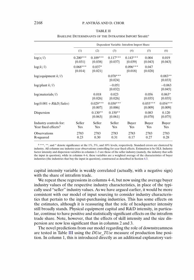
2168 P. ANTRÀS AND D. CHOR
TABLE II
BASELINE DETERMINANTS OF THE INTRAFIRM IMPORT SHAREa
Dependent Variable: Intrafirm Import Share
(1) (2) (3) (4) (5) (6)
log(s/l) 0200*** 0109*** 0117*** 0143*** 0004 0019[0031] [0038] [0037] [0039] [0043] [0043]
log(k/l) 0068*** 0037* 0096*** 0047[0014] [0021] [0018] [0028]
log(equipment k/l) 0070*** 0083**[0024] [0033]
log(plant k/l) −0051 −0063[0032] [0045]
log(materials/l) 0018 0023 0056 0063*[0026] [0026] [0035] [0035]
log(0001 + R&D/Sales) 0029*** 0030*** 0055*** 0054***[0007] [0006] [0009] [0009]
Dispersion 0130** 0150** 0083 0120[0063] [0061] [0070] [0075]
Industry controls for: Seller Seller Seller Buyer Buyer BuyerYear fixed effects? Yes Yes Yes Yes Yes Yes
Observations 2783 2783 2783 2783 2783 2783R-squared 023 030 031 017 027 028
a ***, **, and * denote significance at the 1%, 5%, and 10% levels, respectively. Standard errors are clustered byindustry. All columns use industry-year observations controlling for year fixed effects. Estimation is by OLS. Industryfactor intensity and dispersion variables in columns 1–3 are those of the seller industry (namely, the industry that sellsthe input in question), while in columns 4–6, these variables are a weighted average of the characteristics of buyerindustries (the industries that buy the input in question), constructed as described in Section 4.3.
capital intensity variable is weakly correlated (actually, with a negative sign)with the share of intrafirm trade.
We repeat these regressions in columns 4–6, but now using the average buyerindustry values of the respective industry characteristics, in place of the typi-cally used “seller” industry values. As we have argued earlier, it would be moreconsistent with our model of input sourcing to consider industry characteris-tics that pertain to the input-purchasing industries. This has some effects onthe estimates, although it is reassuring that the role of headquarter intensitystill broadly stands. Physical equipment capital and R&D intensity, in particu-lar, continue to have positive and statistically significant effects on the intrafirmtrade share. Note, however, that the effects of skill intensity and the size dis-persion are now less significant than in columns 2 and 3.
The novel predictions from our model regarding the role of downstreamnessare tested in Table III using the DUse_TUse measure of production line posi-tion. In column 1, this is introduced directly as an additional explanatory vari-
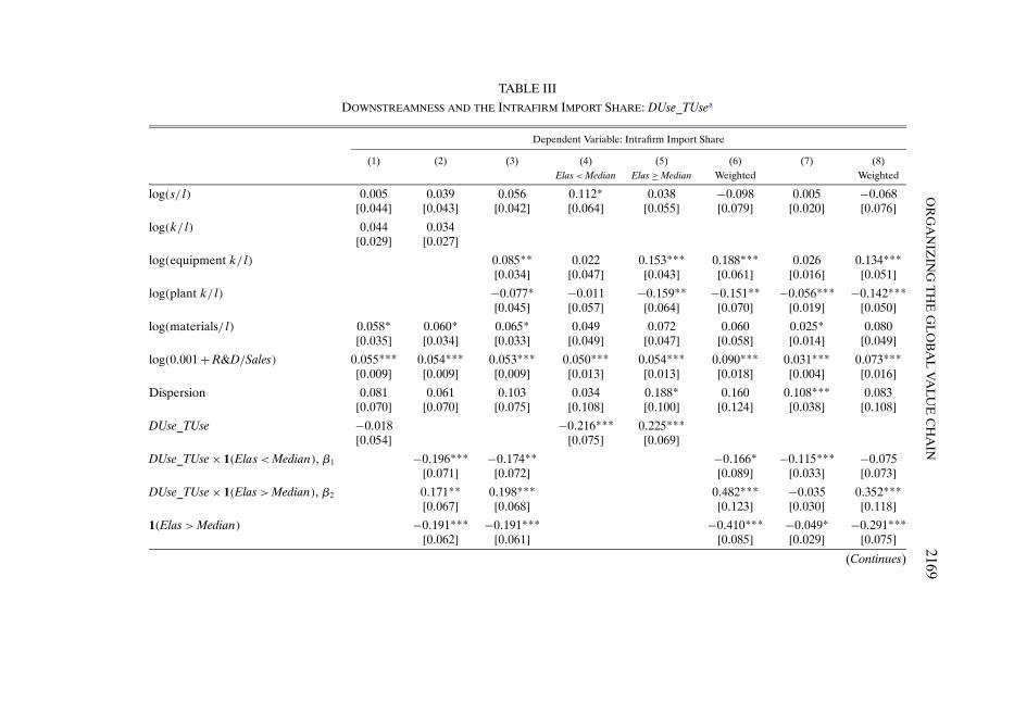
OR
GA
NIZ
ING
TH
EG
LO
BA
LV
AL
UE
CH
AIN
2169TABLE III
DOWNSTREAMNESS AND THE INTRAFIRM IMPORT SHARE: DUse_TUsea
Dependent Variable: Intrafirm Import Share
(1) (2) (3) (4) (5) (6) (7) (8)Elas<Median Elas ≥ Median Weighted Weighted
log(s/l) 0005 0039 0056 0112* 0038 −0098 0005 −0068[0044] [0043] [0042] [0064] [0055] [0079] [0020] [0076]
log(k/l) 0044 0034[0029] [0027]
log(equipment k/l) 0085** 0022 0153*** 0188*** 0026 0134***[0034] [0047] [0043] [0061] [0016] [0051]
log(plant k/l) −0077* −0011 −0159** −0151** −0056*** −0142***[0045] [0057] [0064] [0070] [0019] [0050]
log(materials/l) 0058* 0060* 0065* 0049 0072 0060 0025* 0080[0035] [0034] [0033] [0049] [0047] [0058] [0014] [0049]
log(0001 + R&D/Sales) 0055*** 0054*** 0053*** 0050*** 0054*** 0090*** 0031*** 0073***[0009] [0009] [0009] [0013] [0013] [0018] [0004] [0016]
Dispersion 0081 0061 0103 0034 0188* 0160 0108*** 0083[0070] [0070] [0075] [0108] [0100] [0124] [0038] [0108]
DUse_TUse −0018 −0216*** 0225***[0054] [0075] [0069]
DUse_TUse × 1(Elas <Median), β1 −0196*** −0174** −0166* −0115*** −0075[0071] [0072] [0089] [0033] [0073]
DUse_TUse × 1(Elas>Median), β2 0171** 0198*** 0482*** −0035 0352***[0067] [0068] [0123] [0030] [0118]
1(Elas>Median) −0191*** −0191*** −0410*** −0049* −0291***[0062] [0061] [0085] [0029] [0075]
(Continues)

2170P.A
NT
RÀ
SA
ND
D.C
HO
R
TABLE III—Continued
Dependent Variable: Intrafirm Import Share
(1) (2) (3) (4) (5) (6) (7) (8)Elas<Median Elas ≥ Median Weighted Weighted
p-value: Joint significance of β1 and β2 [00008] [00005] [00000] [00021] [00013]p-value: Test of β2 −β1 = 0 [00002] [00001] [00000] [00595] [00003]Industry controls for: Buyer Buyer Buyer Buyer Buyer Buyer Buyer BuyerYear fixed effects? Yes Yes Yes Yes Yes Yes No NoCountry-year fixed effects? No No No No No No Yes Yes
Observations 2783 2783 2783 1375 1408 2783 270,991 207,991R-squared 027 032 033 037 028 061 018 059
a ***, **, and * denote significance at the 1%, 5%, and 10% levels, respectively. Standard errors are clustered by industry. Columns 1–6 use industry-year observationscontrolling for year fixed effects, while columns 7–8 use country-industry-year observations controlling for country-year fixed effects. Estimation is by OLS. In all columns, theindustry factor intensity and dispersion variables are a weighted average of the characteristics of buyer industries (the industries that buy the input in question), constructed asdescribed in Section 4.3. Columns 4 and 5 restrict the sample to observations where the buyer industry elasticity is smaller (respectively, larger) than the industry median value.“Weighted” columns use the value of total imports for the industry-year or country-industry-year, respectively, as regression weights.

ORGANIZING THE GLOBAL VALUE CHAIN 2171
able in the industry-year regressions.27 When included on its own, the effect ofDUse_TUse on the share of intrafirm trade turns out to be statistically insignif-icant. Following the guidance of our theoretical model, we run our benchmarkspecification from equation (32) in column 2, which includes the interactionsof DUse_TUse with our proxies for the sequential substitutes (Elas<Median)and complements (Elas>Median) cases, as well as a dummy variable for thesequential complements case.28 The empirical results here are indeed stronglysupportive of our model’s central prediction: The effect of downstreamness ispositive and significant at the 5% level when the average buyer demand elas-ticity is above the median for this variable (β2 > 0), consistent with a greaterpropensity toward the integration of input suppliers that enter further down-stream in the value chain. Conversely, the negative and significant β1 coeffi-cient confirms a greater propensity toward integrating upstream productionstages in the sequential substitutes case. As indicated in the table, we can com-fortably reject the null hypothesis that β1 = β2 = 0 (the F-test for joint signifi-cance yields a small p-value of 0.0008), while β2 −β1 is also significantly differ-ent from zero at the 1% level of significance. On a separate note, the effect ofthe (Elas>Median) dummy variable turns out to be negative and statisticallysignificant, which resonates with our comparative static result in Proposition 3on the effect of ρ.
It is particularly reassuring that these new findings stand even while includ-ing the same set of controls for average buyer headquarter intensity and dis-persion that were used earlier in Table II. When we break the physical cap-ital intensity variable in column 3 down into its equipment and plant capitalcomponents, we in fact find that equipment intensity and R&D intensity (twonatural proxies for headquarter intensity) are positively and significantly corre-lated with the intrafirm trade share, consistent with part (ii) of Proposition 4.In Figure 4, we provide further reassurance that our findings are not undulydriven by possible influential observations. After partialing out the effects ofall the control variables used in the column 3 regression, the intrafirm importshare displays a clear upward-sloping relationship with DUse_TUse in the com-plements case (right panel), with a converse slope in the substitutes case (leftpanel).29
The next two columns of Table III verify that the effects we have found inthe pooled sample are also present when we run our regressions separately on
27All our core results reported in Tables III and IV remain very similar if the regressions areinstead run year-by-year, namely, with the intrafirm trade share of industries in a particular yearas the dependent variable, with Huber–White robust standard errors; see Tables S.V and S.VI ofthe Supplemental Material.
28Note that there is no need to include the dummy variable for the sequential substitutes case,as the regressions include a constant term.
29The slope in both of these scatterplots is significantly different from zero at the 1% level(robust standard errors used). The Supplemental Material provides similar figures that illustratethese partial correlations for DownMeasure, as well as for our weighted regression specifications.
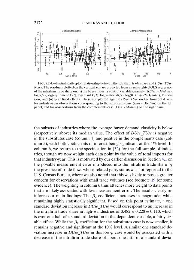
2172 P. ANTRÀS AND D. CHOR
FIGURE 4.—Partial scatterplot relationship between the intrafirm trade share and DUse_TUse.Notes: The residuals plotted on the vertical axis are predicted from an unweighted OLS regressionof the intrafirm trade share on: (i) the buyer industry control variables, namely: 1(Elas>Median),log(s/l), log(equipment k/l), log(plant k/l), log(materials/l), log(0001+R&D/Sales), Disper-sion, and (ii) year fixed effects. These are plotted against DUse_TUse on the horizontal axis,for industry-year observations corresponding to the substitutes case (Elas<Median) on the leftpanel, and for observations from the complements case (Elas>Median) on the right panel.
the subsets of industries where the average buyer demand elasticity is below(respectively, above) its median value. The effect of DUse_TUse is negativein the substitutes case (column 4) and positive in the complements case (col-umn 5), with both coefficients of interest being significant at the 1% level. Incolumn 6, we return to the specification in (32) for the full sample of indus-tries, though we now weight each data point by the value of total imports forthat industry-year. This is motivated by our earlier discussion in Section 4.1 onthe possible measurement error introduced into the intrafirm trade share bythe presence of trade flows whose related party status was not reported to theU.S. Census Bureau, where we also noted that this was likely to pose a greaterconcern for observations with small trade volumes (see footnote 19 for someevidence). The weighting in column 6 thus attaches more weight to data pointsthat are likely associated with less measurement error. The results clearly re-inforce our main findings: The β2 coefficient increases in magnitude, whileremaining highly statistically significant. Based on this point estimate, a onestandard deviation increase in DUse_TUse would correspond to an increase inthe intrafirm trade share in high-ρ industries of 0482 × 0228 = 0110, whichis over one-half of a standard deviation in the dependent variable, a fairly siz-able effect. While the β1 coefficient for the substitutes case is now smaller, itremains negative and significant at the 10% level. A similar one standard de-viation increase in DUse_TUse in this low-ρ case would be associated with adecrease in the intrafirm trade share of about one-fifth of a standard devia-

ORGANIZING THE GLOBAL VALUE CHAIN 2173
tion. Note, too, that the fit of the regression in terms of its R2 also improvesmarkedly under weighted least squares.30
We exploit the additional variation in the intrafirm import share acrosssource countries in the final two columns of Table III. Following the specifi-cation in (33), column 7 includes country-year fixed effects and clusters thestandard errors by industry. Column 8, in turn, weights each observation bythe total import value for that country-industry-year, for reasons analogous tothose discussed above. The unweighted results in column 7 are relatively noisy,while also delivering a low R2. The negative effect of downstreamness on in-tegration remains evident in the substitutes case, but that in the complementscase is now imprecisely estimated (with a sign opposite to that expected fromour model).31 When working with the full country variation, though, there is ar-guably a stronger case for the weighted specification, as there are many moresmall import flow observations and hence a greater scope for measurement er-ror in the intrafirm trade share to matter. These results in column 8, in fact,look very similar to the purely cross-industry findings, with the β2 coefficientpositive and significant at the 1% level, while β1 remains negative (althoughnot statistically significant). The remaining coefficients are also consistent withthe theory, with positive effects for our preferred headquarter intensity mea-sures (equipment capital and R&D intensities), and a negative effect of thedummy variable for the sequential complements case.
In Table IV, we repeat the exercise from Table III using our second down-streamness variable, DownMeasure, in place of DUse_TUse. This reassuringlycorroborates our earlier findings on how production line position influences in-tegration outcomes, particularly in the complements case. We consistently finda positive and significant effect of DownMeasure on the propensity to importgoods within firm boundaries in the high-ρ case, both in the specifications thatpool all industries (columns 2, 3, 6) and when we focus on the subset of indus-tries with above-median average buyer demand elasticities (column 5). This ef-fect is especially strong when we weight observations by import volumes: basedon column 6, a one standard deviation increase in DownMeasure would imply arise in the intrafirm import share of 0526 × 0222 = 0117, which is once againjust over half a standard deviation for our dependent variable. We likewise ob-tain a similar set of results in column 8, which uses the country-industry-yeardata with weighted least squares. Admittedly, the evidence in Table IV is more
30One might be concerned that the largest manufacturing industry by import value, IO 336311(Automobile), is also the most downstream according to both DUse_TUse and DownMeasure, andthat this might be driving the significant findings in the weighted regressions. Our results remainqualitatively similar and significant when dropping this industry, in both the cross-industry andthe cross-industry, cross-country specifications (available on request).
31Note, nevertheless, that these point estimates are still consistent with the weaker predictionthat downstreamness should have a more negative effect on integration in the substitutes than inthe complements case. Formally, we can reject the null hypothesis that the two coefficients areequal (β1 = β2) at the 10% level of significance.
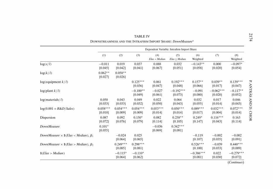
2174P.A
NT
RÀ
SA
ND
D.C
HO
R
TABLE IV
DOWNSTREAMNESS AND THE INTRAFIRM IMPORT SHARE: DownMeasurea
Dependent Variable: Intrafirm Import Share
(1) (2) (3) (4) (5) (6) (7) (8)Elas<Median Elas ≥ Median Weighted Weighted
log(s/l) −0011 0019 0037 0088 0032 −0143** 0000 −0097*[0045] [0042] [0041] [0067] [0051] [0058] [0020] [0054]
log(k/l) 0062** 0058**[0027] [0026]
log(equipment k/l) 0125*** 0061 0192*** 0157** 0039** 0139***[0036] [0047] [0048] [0066] [0017] [0047]
log(plant k/l) −0100** −0027 −0192*** −0091 −0062*** −0117**[0049] [0061] [0073] [0080] [0020] [0052]
log(materials/l) 0050 0043 0049 0022 0064 0032 0017 0046[0033] [0033] [0032] [0050] [0043] [0055] [0014] [0043]
log(0001 + R&D/Sales) 0058*** 0054*** 0054*** 0053*** 0050*** 0089*** 0032*** 0072***[0010] [0009] [0009] [0014] [0014] [0017] [0004] [0014]
Dispersion 0087 0092 0150* 0082 0258** 0249* 0116*** 0163[0072] [0076] [0079] [0114] [0105] [0147] [0043] [0114]
DownMeasure 0101* −0036 0342***[0055] [0069] [0081]
DownMeasure × 1(Elas<Median), β1 −0024 0025 −0119 −0002 −0002[0064] [0065] [0107] [0035] [0091]
DownMeasure × 1(Elas>Median), β2 0249*** 0298*** 0526*** −0039 0440***[0085] [0081] [0100] [0033] [0089]
1(Elas>Median) −0115* −0110* −0386*** 0022 −0279***[0064] [0062] [0081] [0030] [0072]
(Continues)

OR
GA
NIZ
ING
TH
EG
LO
BA
LV
AL
UE
CH
AIN
2175
TABLE IV—Continued
Dependent Variable: Intrafirm Import Share
(1) (2) (3) (4) (5) (6) (7) (8)Elas<Median Elas ≥ Median Weighted Weighted
p-value: Joint significance of β1 and β2 [00138] [00013] [00000] [04995] [00000]p-value: Test of β2 −β1 = 0 [00103] [00067] [00000] [04180] [00001]Industry controls for: Buyer Buyer Buyer Buyer Buyer Buyer Buyer BuyerYear fixed effects? Yes Yes Yes Yes Yes Yes No NoCountry-year fixed effects? No No No No No No Yes Yes
Observations 2783 2783 2783 1375 1408 2783 207,991 207,991R-squared 028 031 033 033 033 064 018 061
a ***, **, and * denote significance at the 1%, 5%, and 10% levels, respectively. Standard errors are clustered by industry. Columns 1–6 use industry-year observationscontrolling for year fixed effects, while columns 7–8 use country-industry-year observations controlling for country-year fixed effects. Estimation is by OLS. In all columns, theindustry factor intensity and dispersion variables are a weighted average of the characteristics of buyer industries (the industries that buy the input in question), constructed asdescribed in Section 4.3. Columns 4 and 5 restrict the sample to observations where the buyer industry elasticity is smaller (respectively, larger) than the industry median value.“Weighted” columns use the value of total imports for the industry-year or country-industry-year, respectively, as regression weights.

2176 P. ANTRÀS AND D. CHOR
mixed with regard to the role of DownMeasure for industries that fall under thesubstitutes case. The overall results do point toward a negative effect, althoughthe point estimates are much smaller and not statistically distinguishable fromzero. Still, the difference between β1 and β2 remains statistically significant atconventional levels.
5.2. Alternative Specifications
We turn next to address potential criticisms regarding the use of a mediancutoff value for the ρ proxy to distinguish between the sequential substitutesand complements cases. Given that technological substitutability (α in ourmodel) might well vary across sectors, it would be reasonable to expect thatthe positive effects of downstreamness would be concentrated in the high-est ranges of the elasticity demand parameter ρ, while the negative effects ofdownstreamness might only be evident for particularly low values of ρ. Thisleads us to consider a more flexible variant of (32) that breaks down our em-pirical proxy for ρ by quintiles:
Sit =5∑s=1
βsDi × 1(ρi ∈Ωρ�s)+5∑s=2
γs1(ρi ∈Ωρ�s)+βXXi + αt + εit (34)
Here, Ωρ�s refers to the subset corresponding to the sth quintile of ρ (fors = 1�2� �5), with 1(ρi ∈ Ωρ�s) being a dummy variable equal to 1 if in-dustry i falls within this sth quintile.32 We report three regressions in Table Vfor each of the downstreamness variables, DUse_TUse and DownMeasure. Foreach measure, we estimate (34) both without and with regression weights in thefirst and second columns, respectively; the third column then runs the analo-gous weighted specification with the country-industry-year data, while control-ling for country-year fixed effects. (For all regressions reported in the remain-der of this paper, standard errors will be clustered by industry; the full set ofaverage buyer industry variables used in column 3 in Tables III and IV will alsobe included as controls.)
Table V confirms that the effect of downstreamness on the intrafirm importshare differs qualitatively depending on the average buyer demand elasticity.The point estimates obtained on the downstreamness variables in the lower(first and second) quintiles of the ρ proxy are negative, barring a few excep-tions, even being significant at the 10% level in two of the DUse_TUse speci-fications. These coefficients progressively increase as we move from β1 in thelowest quintile to β5 in the highest, eventually becoming positive and statis-tically significant in all columns in the fifth quintile of ρ, precisely for those
32We drop the level effect of the first quintile dummy, as the regression already includes aconstant term.
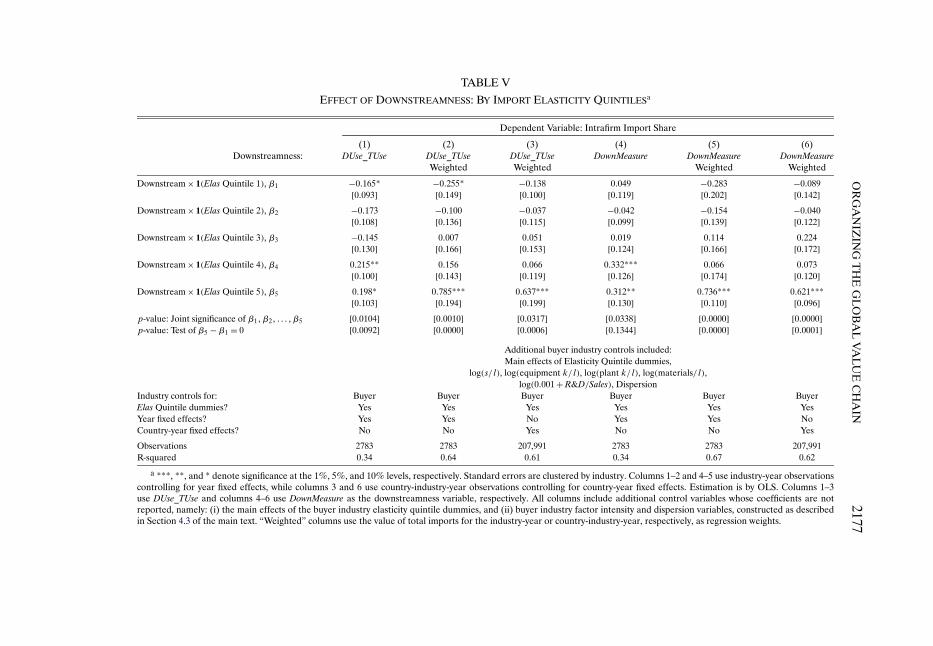
OR
GA
NIZ
ING
TH
EG
LO
BA
LV
AL
UE
CH
AIN
2177TABLE V
EFFECT OF DOWNSTREAMNESS: BY IMPORT ELASTICITY QUINTILESa
Dependent Variable: Intrafirm Import Share
(1) (2) (3) (4) (5) (6)Downstreamness: DUse_TUse DUse_TUse DUse_TUse DownMeasure DownMeasure DownMeasure
Weighted Weighted Weighted Weighted
Downstream × 1(Elas Quintile 1), β1 −0165* −0255* −0138 0049 −0283 −0089[0093] [0149] [0100] [0119] [0202] [0142]
Downstream × 1(Elas Quintile 2), β2 −0173 −0100 −0037 −0042 −0154 −0040[0108] [0136] [0115] [0099] [0139] [0122]
Downstream × 1(Elas Quintile 3), β3 −0145 0007 0051 0019 0114 0224[0130] [0166] [0153] [0124] [0166] [0172]
Downstream × 1(Elas Quintile 4), β4 0215** 0156 0066 0332*** 0066 0073[0100] [0143] [0119] [0126] [0174] [0120]
Downstream × 1(Elas Quintile 5), β5 0198* 0785*** 0637*** 0312** 0736*** 0621***[0103] [0194] [0199] [0130] [0110] [0096]
p-value: Joint significance of β1�β2� �β5 [00104] [00010] [00317] [00338] [00000] [00000]p-value: Test of β5 −β1 = 0 [00092] [00000] [00006] [01344] [00000] [00001]
Additional buyer industry controls included:Main effects of Elasticity Quintile dummies,
log(s/l), log(equipment k/l), log(plant k/l), log(materials/l),log(0001 + R&D/Sales), Dispersion
Industry controls for: Buyer Buyer Buyer Buyer Buyer BuyerElas Quintile dummies? Yes Yes Yes Yes Yes YesYear fixed effects? Yes Yes No Yes Yes NoCountry-year fixed effects? No No Yes No No Yes
Observations 2783 2783 207,991 2783 2783 207,991R-squared 034 064 061 034 067 062
a ***, **, and * denote significance at the 1%, 5%, and 10% levels, respectively. Standard errors are clustered by industry. Columns 1–2 and 4–5 use industry-year observationscontrolling for year fixed effects, while columns 3 and 6 use country-industry-year observations controlling for country-year fixed effects. Estimation is by OLS. Columns 1–3use DUse_TUse and columns 4–6 use DownMeasure as the downstreamness variable, respectively. All columns include additional control variables whose coefficients are notreported, namely: (i) the main effects of the buyer industry elasticity quintile dummies, and (ii) buyer industry factor intensity and dispersion variables, constructed as describedin Section 4.3 of the main text. “Weighted” columns use the value of total imports for the industry-year or country-industry-year, respectively, as regression weights.

2178 P. ANTRÀS AND D. CHOR
industries most likely to fall under the sequential complements case. Collec-tively, we find that the coefficients of downstreamness over these five quintilesare jointly significant, while the difference β5 − β1 is also significantly differ-ent from zero at the 1% level except in one specification (column 4). Theseresults, therefore, strengthen our confidence in the empirical relevance of ourkey theoretical predictions.
We further seek to allay concerns regarding omitted variables bias, specifi-cally those arising from other industry characteristics that could affect the in-trafirm trade share which we have not explicitly controlled for so far. Towardthis end, we revert to our cross-industry specification in equation (32) and in-troduce several plausible controls; these results are reported in Table VI forDUse_TUse and in Table VII for DownMeasure.33 We control for the value-added content of each industry—the ratio of value-added to total shipments—in column 1. Column 2 examines whether the importance of a good as an inputin production processes might have an effect on the propensity to trade thatgood within firm boundaries. We capture this through a measure equal to thevalue of an industry’s total use as an input, divided by the total input pur-chases made by all its buyer industries, constructed from the 2002 U.S. Input–Output Tables.34 We incorporate the intermediation variable from Bernard etal. (2010) in column 3, this being a measure of the extent to which wholesalersthat serve as intermediaries to transactions are observed to be active in a givenindustry. Finally, column 4 controls for proxies for industry contractibility, assuggested by Nunn and Trefler (2008). These are based on the underlying shareof products from an industry that are transacted on organized exchanges or arereference-priced according to Rauch (1999), and which thus can be regardedas homogeneous and readily contractible goods.35 We control here for both theown contractibility of the good in question as well as an average contractibil-ity taken over industries that purchase the good, so as to distinguish betweencontracting frictions inherent to the seller and average buyer industries, re-spectively. (Further details on the construction of these additional variablescan be found in the Data Appendix.)
Our central finding on the contrasting effects of downstreamness in the sub-stitutes versus complements case turns out to be remarkably robust. This is
33We have also run these same robustness checks on the full country-industry-year data, usingthe specification in (33). These results are reported in Tables S.VII and S.VIII of the Supple-mental Material, respectively, for DUse_TUse and DownMeasure, for the weighted least squaresregressions. We consistently obtain results akin to our baselines: a positive and significant effectof downstreamness in the complements case, and a negative (albeit insignificant) effect in thesubstitutes case.
34The robustness results are very similar if we alternatively divide by the total gross output ofbuyer industries when constructing this input “importance” variable (available on request).
35We report results using the liberal classification in Rauch (1999). The findings are very similarwhen using his conservative classification, or when excluding reference-priced products from thedefinition of what constitutes a contractible good (results available on request).
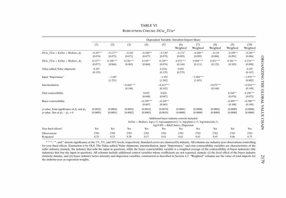
OR
GA
NIZ
ING
TH
EG
LO
BA
LV
AL
UE
CH
AIN
2179TABLE VI
ROBUSTNESS CHECKS: DUse_TUsea
Dependent Variable: Intrafirm Import Share
(1) (2) (3) (4) (5) (6) (7) (8) (9) (10)Weighted Weighted Weighted Weighted Weighted
DUse_TUse × 1(Elas<Median), β1 −0187** −0177** −0103 −0180** −0130* −0171* −0188** −0119 −0199** −0185**[0074] [0072] [0071] [0077] [0079] [0093] [0093] [0080] [0091] [0084]
DUse_TUse × 1(Elas<Median), β2 0157** 0198*** 0236*** 0159** 0158** 0472*** 0504*** 0451*** 0391*** 0374***[0077] [0068] [0065] [0068] [0074] [0144] [0111] [0125] [0103] [0090]
Value-added/Value shipments 0187 0216∗ 0054 0107[0135] [0125] [0275] [0167]
Input “Importance” −1687 −1453 −3484*** −3975***[1231] [1302] [1021] [0802]
Intermediation −0464*** −0413*** −0673*** −0654***[0106] [0102] [0168] [0149]
Own contractibility 0019 0024 0184** 0198***[0048] [0047] [0076] [0075]
Buyer contractibility −0199*** −0169** −0499*** −0508***[0067] [0065] [0108] [0109]
p-value: Joint significance of β1 and β2 [00022] [00004] [00003] [00012] [00074] [00001] [00000] [00002] [00000] [00000]p-value: Test of β2 −β1 = 0 [00005] [00001] [00002] [00003] [00019] [00000] [00000] [00000] [00000] [00000]
Additional buyer industry controls included:1(Elas>Median), log(s/l), log(equipment k/l), log(plant k/l), log(materials/l),
log(0001 + R&D/Sales), DispersionYear fixed effects? Yes Yes Yes Yes Yes Yes Yes Yes Yes Yes
Observations 2783 2783 2783 2783 2783 2783 2783 2783 2783 2783R-squared 033 033 038 037 041 061 063 065 066 073
a ***, **, and * denote significance at the 1%, 5%, and 10% levels, respectively. Standard errors are clustered by industry. All columns use industry-year observations controllingfor year fixed effects. Estimation is by OLS. The Value-added/Value shipments, intermediation, input “Importance,” and own contractibility variables are characteristics of theseller industry (namely, the industry that sells the input in question), while the buyer contractibility variable is a weighted average of the contractibility of buyer industries (theindustries that buy the input in question). All columns include additional control variables whose coefficients are not reported, namely: (i) the level effect of the buyer industryelasticity dummy, and (ii) buyer industry factor intensity and dispersion variables, constructed as described in Section 4.3. “Weighted” columns use the value of total imports forthe industry-year as regression weights.

2180P.A
NT
RÀ
SA
ND
D.C
HO
R
TABLE VII
ROBUSTNESS CHECKS: DownMeasurea
Dependent Variable: Intrafirm Import Share
(1) (2) (3) (4) (5) (6) (7) (8) (9) (10)Weighted Weighted Weighted Weighted Weighted
DownMeasure × 1(Elas<Median), β1 0014 0021 0083 0007 0046 −0137 −0152 −0040 −0213** −0216**[0067] [0065] [0062] [0067] [0065] [0110] [0110] [0101] [0103] [0099]
DownMeasure × 1(Elas<Median), β2 0277*** 0294*** 0310*** 0284*** 0270*** 0515*** 0505*** 0500*** 0442*** 0371***[0084] [0081] [0076] [0075] [0075] [0098] [0098] [0097] [0084] [0066]
Value-added/Value shipments 0168 0235* 0331 −0599***[0130] [0120] [0208] [0150]
Input “Importance” −0954 −0866 −1565* −2805***[1351] [1403] [0806] [0633]
Intermediation −0488*** −0443*** −0652*** −0599***[0104] [0103] [0161] [0150]
Own contractibility 0062 0059 0204*** 0211***[0046] [0044] [0077] [0064]
Buyer contractibility −0238*** −0197*** −0509*** −0514***[0065] [0063] [0110] [0102]
p-value: Joint significance of β1 and β2 [00050] [00015] [00002] [00009] [00018] [00000] [00000] [00000] [00000] [00000]p-value: Test of β2 −β1 = 0 [00102] [00066] [00170] [00039] [00169] [00000] [00000] [00000] [00000] [00000]
Additional buyer industry controls included:1(Elas>Median), log(s/l), log(equipment k/l), log(plant k/l), log(materials/l),
log(0001 + R&D/Sales), DispersionYear fixed effects? Yes Yes Yes Yes Yes Yes Yes Yes Yes Yes
Observations 2783 2783 2783 2783 2783 2783 2783 2783 2783 2783R-squared 033 039 033 037 042 065 068 065 069 075
a ***, **, and * denote significance at the 1%, 5%, and 10% levels, respectively. Standard errors are clustered by industry. All columns use industry-year observations controllingfor year fixed effects. Estimation is by OLS. The Value-added/Value shipments, intermediation, input “Importance,” and own contractibility variables are characteristics of theseller industry (namely, the industry that sells the input in question), while the buyer contractibility variable is a weighted average of the contractibility of buyer industries (theindustries that buy the input in question). All columns include additional control variables whose coefficients are not reported, namely: (i) the level effect of the buyer industryelasticity dummy, and (ii) buyer industry factor intensity and dispersion variables, constructed as described in Section 4.3. “Weighted” columns use the value of total imports forthe industry-year as regression weights.

ORGANIZING THE GLOBAL VALUE CHAIN 2181
true when we introduce the aforementioned additional industry variables ei-ther individually (columns 1–4) or jointly (column 5), as well as when we runthe regressions using total imports as weights (columns 6–10). Throughout Ta-ble VI, DUse_TUse consistently has a negative correlation with the intrafirmtrade share in the low-ρ case, with this coefficient being significant at least atthe 10% level except in columns 3 and 8 where we control for the intermedi-ation variable on its own. On the other hand, the positive correlation for thehigh-ρ case is always significant at the 5% level. We also obtain results simi-lar to our baseline regressions when using DownMeasure instead in Table VII.Once again, we find that downstreamness is strongly associated with a higherintrafirm trade share in the complements case, although the coefficients for thesubstitutes case remain, for the most part, imprecisely estimated.
Of independent interest, the intermediation variable always shows up witha negative and highly significant coefficient when included. This is consistentwith Bernard et al. (2010), who interpreted the presence of wholesale interme-diation as indicative of a reduced need to expand the boundaries of the firmto secure the input in question. Separately, in the columns that control for therole of contracting frictions, we generally find that inputs that are more con-tractible appear to be transacted more within firm boundaries, while a greaterdegree of buyer industry contractibility is associated with a reduced propen-sity toward integration, with these correlations being particularly strong in theweighted specifications.36 In the case of DownMeasure, the negative coefficienton downstreamness in the substitutes case even becomes statistically significantin columns 9–10.37
5.3. Extensions
We round off our empirical analysis by testing several auxiliary implicationsfrom the extensions that we developed in Sections 3.2–3.4, in order to explorehow far the patterns in the data are consistent with these additional predictionsof our model of sequential production and sourcing.
Table VIII examines further the role of headquarter intensity. In Section 3.2,we showed that an increase in η not only expands the range of stages that arevertically integrated, but also affects the range of parameter values for whichdownstreamness is predicted to have a positive effect on the share of intrafirm
36Incidentally, this dovetails with the predictions of the theoretical model in Antràs and Help-man (2008) which introduced a formulation of partial input contractibility; see, in particular, theirProposition 5.
37In regressions that use the additional source country dimension in the intrafirm import share,Nunn and Trefler (2008) have further interacted the industry contractibility variables with a coun-try index of the rule of law to get a richer proxy for contracting frictions. We have done the sameusing the most updated version of the rule of law index from Kaufmann, Kraay, and Mastruzzi(2010), and verified that this does not affect our main findings at all (see column 5 in Tables S.VIIand S.VIII of the Supplemental Material).
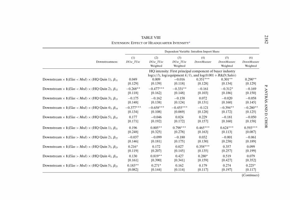
2182P.A
NT
RÀ
SA
ND
D.C
HO
R
TABLE VIII
EXTENSION: EFFECT OF HEADQUARTER INTENSITYa
Dependent Variable: Intrafirm Import Share
(1) (2) (3) (4) (5) (6)Downstreamness: DUse_TUse DUse_TUse DUse_TUse DownMeasure DownMeasure DownMeasure
Weighted Weighted Weighted Weighted
HQ intensity: First principal component of buyer industrylog(s/l), log(equipment k/l), and log(0001 + R&D/Sales)
Downstream × 1(Elas<Med)× (HQ Quin 1), β11 0049 0009 −0016 0351*** 0301** 0290**[0129] [0139] [0118] [0128] [0134] [0129]
Downstream × 1(Elas<Med)× (HQ Quin 2), β12 −0268** −0477*** −0331** −0161 −0312* −0169[0118] [0162] [0148] [0103] [0186] [0150]
Downstream × 1(Elas<Med)× (HQ Quin 3), β13 −0175 −0162 −0158 0072 −0020 −0058[0148] [0138] [0124] [0131] [0160] [0145]
Downstream × 1(Elas<Med)× (HQ Quin 4), β14 −0377*** −0658*** −0455*** −0121 −0394** −0280**[0134] [0108] [0069] [0128] [0172] [0125]
Downstream × 1(Elas<Med)× (HQ Quin 5), β15 0177 −0046 0024 0229 −0181 −0050[0171] [0192] [0172] [0157] [0160] [0158]
Downstream × 1(Elas>Med)× (HQ Quin 1), β21 0196 0805** 0798*** 0465*** 0624*** 0593***[0248] [0325] [0278] [0163] [0113] [0087]
Downstream × 1(Elas>Med)× (HQ Quin 2), β22 −0037 −0099 −0180 0032 −0001 −0061[0146] [0181] [0175] [0130] [0238] [0189]
Downstream × 1(Elas>Med)× (HQ Quin 3), β23 0216* 0172 0027 0358*** 0357 0099[0119] [0207] [0145] [0135] [0257] [0199]
Downstream × 1(Elas>Med)× (HQ Quin 4), β24 0130 0819** 0427 0280* 0519 0079[0161] [0390] [0341] [0159] [0427] [0352]
Downstream × 1(Elas>Med)× (HQ Quin 5), β25 0183** 0271* 0162 0179 0274 0225*[0082] [0144] [0114] [0117] [0197] [0117]
(Continues)

OR
GA
NIZ
ING
TH
EG
LO
BA
LV
AL
UE
CH
AIN
2183
TABLE VIII—Continued
Dependent Variable: Intrafirm Import Share
(1) (2) (3) (4) (5) (6)Downstreamness: DUse_TUse DUse_TUse DUse_TUse DownMeasure DownMeasure DownMeasure
Weighted Weighted Weighted Weighted
p-value: Joint significance of β11� �β15�β21� �β25 [00065] [00000] [00000] [00004] [00000] [00000]p-value: Test of β11 −β15 = 0 [05271] [08062] [08438] [05397] [00182] [00833]p-value: Test of β21 −β25 = 0 [09599] [01790] [00477] [01699] [01921] [00262]
Additional buyer industry controls included:Main and double interaction effects,
log(s/l), log(equipment k/l), log(plant k/l), log(materials/l),log(0001 + R&D/Sales), Dispersion
Main and double interaction effects? Yes Yes Yes Yes Yes YesYear fixed effects? Yes Yes No Yes Yes NoCountry-year fixed effects? No No Yes No No Yes
Observations 2783 2783 207,991 2783 2783 207,991R-squared 040 069 063 040 071 065
a ***, **, and * denote significance at the 1%, 5%, and 10% levels, respectively. Standard errors are clustered by industry. Columns 1–2 and 4–5 use industry-year observationscontrolling for year fixed effects, while columns 3 and 6 use country-industry-year observations controlling for country-year fixed effects. Estimation is by OLS. Columns 1–3 useDUse_TUse and columns 4–6 use DownMeasure as the downstreamness variable, respectively. The hq intensity measure is the first principal component of the buyer industry’slog(s/l), log(equipment k/l), and log(0001 + R&D/Sales). All columns include additional control variables whose coefficients are not reported, namely: (i) the main and doubleinteraction effects of the buyer industry elasticity dummies and hq intensity quintile dummies, and (ii) buyer industry factor intensity and dispersion variables, constructed asdescribed in Section 4.3. “Weighted” columns use the value of total imports for the industry-year or country-industry-year, respectively, as regression weights.

2184 P. ANTRÀS AND D. CHOR
trade. In particular, recall from Proposition 4 that the complements and sub-stitutes cases are now defined by ρ̃≡ (1−η)ρ > α and ρ̃ < α, respectively, andthus the larger η is, the less likely it is that downstreamness will have a positiveeffect on the intrafirm trade share, even for large values of the buyer demandelasticity ρ.
The findings from Table VIII uncover some evidence of this. The key differ-ence relative to the specifications in (32) and (33) is that we now include tripleinteractions, betweenDi×1(ρi < ρmed) andDi×1(ρi > ρmed) on the one hand,and a set of five dummy variables corresponding to the quintiles of a summarymeasure of headquarter intensity on the other. The latter is computed as thefirst principal component of the three main industry measures of headquarterintensity that we have been using, namely, the average buyer skill, equipmentcapital, and R&D intensities. We report three specifications in Table VIII foreach downstreamness measure, namely, an unweighted cross-industry regres-sion, a weighted cross-industry regression, as well as a weighted cross-country,cross-industry regression. (Throughout, we also control for the main and dou-ble interaction effects of the terms in our triple interactions.) We find herethat the positive effect of Di × 1(ρi > ρmed) on the intrafirm trade share is con-centrated in the lowest quintile of headquarter intensity, with few systematicpatterns apparent for the other quintiles of our composite proxy for η. Thereis some evidence also that the negative effect of Di × 1(ρi < ρmed) is strongestin a relatively high (fourth) quintile of η; the coefficients in the fifth quintileare generally negative, though admittedly not significant.38
We turn in Table IX to an implication of the model that arises from incor-porating firm heterogeneity in Section 3.3. As anticipated there, to the extentthat the fixed costs of integration are relatively high, only the most downstreamof stages would be integrated in the sequential complements case, with theconverse prediction (integration of the most upstream stages) applying in thesubstitutes case. We thus attempt to capture these predictions, by replacingour two main interaction terms in (32) and (33) with quintiles of Di inter-acted with each of 1(ρi > ρmed) and 1(ρi < ρmed).39 These results are presentedin Table IX, where the columns correspond to the same estimation proceduresused previously in Table VIII for DUse_TUse (columns 1–3) and DownMeasure(columns 4–6). We indeed find throughout all six columns that the positive ef-fect of downstreamness on the intrafirm import share is concentrated in thehighest quintile of Di in the high-ρ case. Moreover, in the low-ρ case, the
38These qualitative patterns should be taken with a pinch of salt. We are not able to consistentlyreject across all the specifications the hypothesis that the coefficients of Di × 1(ρi > ρmed) in thehighest and lowest headquarter intensity quintiles are in fact equal; a similar caveat applies to thecoefficients for the substitutes case.
39We drop one of these interactions due to the collinearity with the constant term in the re-gressions.

OR
GA
NIZ
ING
TH
EG
LO
BA
LV
AL
UE
CH
AIN
2185
TABLE IX
EXTENSION: IMPLICATIONS OF FIRM HETEROGENEITYa
Dependent Variable: Intrafirm Import Share
(1) (2) (3) (4) (5) (6)Downstreamness: DUse_TUse DUse_TUse DUse_TUse DownMeasure DownMeasure DownMeasure
Weighted Weighted Weighted Weighted
(Downstream Quin 1) × 1(Elas<Median), β11 0101** 0210*** 0145*** 0060 0184*** 0145**[0045] [0058] [0045] [0051] [0067] [0059]
(Downstream Quin 2) × 1(Elas<Median), β12 0041 0131** 0096* −0005 0062 0019[0043] [0062] [0054] [0045] [0069] [0055]
(Downstream Quin 3) × 1(Elas<Median), β13 0008 0063 0010 −0016 0089 0049[0046] [0057] [0046] [0049] [0076] [0060]
(Downstream Quin 4) × 1(Elas<Median), β14 −0047 0092 0047 0024 0064 0032[0043] [0065] [0051] [0045] [0075] [0058]
(Downstream Quin 5) × 1(Elas<Median), β15 0017 0084 0082 0023 0039 0058[0042] [0063] [0053] [0042] [0081] [0064]
(Downstream Quin 2) × 1(Elas>Median), β22 0021 0031 0016 0013 −0054 −0068[0036] [0067] [0056] [0039] [0069] [0052]
(Downstream Quin 3)× 1(Elas>Median), β23 0086** 0150** 0072 0035 0076 0018[0044] [0065] [0052] [0047] [0069] [0066]
(Downstream Quin 4) × 1(Elas>Median), β24 0030 0086 0017 0073* 0056 0013[0048] [0056] [0050] [0043] [0072] [0060]
(Downstream Quin 5) × 1(Elas>Median), β25 0181*** 0352*** 0257*** 0171*** 0380*** 0300***[0048] [0067] [0062] [0059] [0085] [0074]
(Continues)

2186P.A
NT
RÀ
SA
ND
D.C
HO
R
TABLE IX—Continued
Dependent Variable: Intrafirm Import Share
(1) (2) (3) (4) (5) (6)Downstreamness: DUse_TUse DUse_TUse DUse_TUse DownMeasure DownMeasure DownMeasure
Weighted Weighted Weighted Weighted
p-value: Joint significance of β11� �β15�β21� �β25 [00002] [00000] [00000] [00607] [00000] [00000]p-value: Test of β11 −β15 = 0 [00644] [00530] [01986] [04766] [00278] [01006]p-value: Test of β25 = 0 [00002] [00000] [00000] [00043] [00000] [00001]
Additional buyer industry controls included:Main effects of Downstreamness Quintiles and Elasticity dummies,
log(s/l), log(equipment k/l), log(plant k/l), log(materials/l),log(0001 + R&D/Sales), Dispersion
Downstream Quin and Elasticity dummies? Yes Yes Yes Yes Yes YesYear fixed effects? Yes Yes No Yes Yes NoCountry-year fixed effects? No No Yes No No Yes
Observations 2783 2783 207,991 2783 2783 207,991R-squared 035 063 061 033 067 063
a ***, **, and * denote significance at the 1%, 5%, and 10% levels, respectively. Standard errors are clustered by industry. Columns 1–2 and 4–5 use industry-year observationscontrolling for year fixed effects, while columns 3 and 6 use country-industry-year observations controlling for country-year fixed effects. Estimation is by OLS. Columns 1–3 useDUse_TUse and columns 4–6 use DownMeasure as the downstreamness variable, respectively. All columns include additional control variables whose coefficients are not reported,namely: (i) the main effects of the downstreamness quintile dummies and the buyer industry elasticity dummies, and (ii) buyer industry factor intensity and dispersion variables,constructed as described in Section 4.3. “Weighted” columns use the value of total imports for the industry-year or country-industry-year, respectively, as regression weights.
ORGANIZING THE GLOBAL VALUE CHAIN 2187
propensity toward integration is strongest in the lowest quintile of Di.40 Ta-ble IX thus provides strong evidence consistent with this further predictionfrom our model.
In Table X, we seek to correct our cross-country, cross-industry regressionsfor potential selection bias. As explained in Section 3.4, controlling for countryfixed effects may not be sufficient for this purpose when the location of inputproduction is itself affected by the level of downstreamness. For this reason,we carry out a two-stage Heckman selection procedure in Table X that seeks tocorrect for selection into foreign sourcing. In the context of our data set, obser-vations for which no imports were observed entering the United States are nec-essarily dropped from our regression sample, since the denominator of the in-trafirm import share would equal zero in these cases. Any bias that might arisewould, moreover, be more salient in the specifications that incorporate the fullcross-country variation, since up to 60% of all potential country-industry-yearobservations are, in fact, zero import flows, and hence are dropped. To addressthis, we adopt as selection variables (to be included only in the first stage)an interaction term between an indicator for whether countries have abovesample-median entry costs (taken from the Doing Business data set) and theselling industry’s R&D intensity. This country measure of entry costs is specif-ically the first principal component of the number of procedures, number ofdays, and the cost (as a percentage of income per capita) incurred to legallystart a local business. (Note, however, that a number of countries have to bedropped due to the lack of entry cost data.) We, in turn, view the seller in-dustry R&D variable as a proxy for high fixed costs particularly at the entrystage.41 Following the logic of Helpman, Melitz, and Rubinstein (2008), thelevel of such country-industry entry costs can be expected to affect the entrydecisions of firms, and thus to also be positively correlated with the fixed coststhat would be associated with expanding a firm to engage in export activities tothe United States. In contrast, these entry costs are less likely to directly shapethe intensive margin of trade.42
40In this low-ρ case, the difference between the coefficients of Di in the highest and lowestquintiles is marginally significant at the 10% level in three out of the six columns. On the otherhand, for the high-ρ case, the effect of downstreamness in its highest quintile is always signifi-cantly different from that in its lowest quintile (the latter effect having been normalized to zero).
41In unreported results, we have also experimented with measures of industry scale economiescalculated as the employment per establishment, drawn from the U.S. Census Bureau’s CountyBusiness Patterns data set. Our conclusions are largely unaffected with such alternative proxiesof industry fixed costs.
42International tax considerations are often seen as another key factor that influences entrydecisions by multinational firms. We have nevertheless verified that our results from specification(33) remain very similar when we restrict our sample to countries whose effective corporate taxrates for U.S. multinationals were within a 5% range of that for these multinationals’ domesticU.S. activities, based on a 2011 PriceWaterhouseCoopers survey canvassing U.S. firms entitled“Global Effective Tax Rates.” We thank Brent Neiman for bringing this survey to our attention.

2188P.A
NT
RÀ
SA
ND
D.C
HO
R
TABLE X
SELECTION INTO INTRAFIRM TRADEa
Dependent Variable: Intrafirm Import Share
(1) (2) (3) (4) (5) (6)Downstreamness: DUse_TUse DUse_TUse DUse_TUse DownMeasure DownMeasure DownMeasure
Weighted Weighted Weighted Weighted
log(s/l) 0424** −0079 −0072 0343** −0107** −0104**[0166] [0065] [0059] [0167] [0048] [0050]
log(equipment k/l) −0084 0131*** 0130*** −0056 0125*** 0124***[0203] [0040] [0041] [0176] [0040] [0041]
log(plant k/l) −0026 −0139*** −0140*** −0030 −0113** −0113**[0234] [0046] [0046] [0217] [0049] [0048]
log(materials/l) −0083 0063 0061 −0098 0042 0040[0136] [0043] [0042] [0133] [0042] [0041]
Buyer log(0001 + R&D/Sales) −0015 0080*** 0080*** 0001 0080*** 0080***[0064] [0014] [0014] [0061] [0014] [0014]
Dispersion −0234 0117 0113 −0284 0178 0175[0405] [0104] [0104] [0392] [0115] [0117]
Downstream × 1(Elas<Median), β1 0047 −0073 −0072 0634** −0020 −0011[0310] [0074] [0074] [0317] [0097] [0088]
Downstream × 1(Elas>Median), β2 0274 0310*** 0314*** −0291 0353*** 0347***[0252] [0106] [0102] [0246] [0078] [0084]
1(Elas>Median) 0003 −0268*** −0268*** 0661*** −0244*** −0234***[0231] [0075] [0075] [0233] [0076] [0073]
Seller log(0001 + R&D/Sales) −0028*** −0028***× Country Entry Costs [0007] [0007]
Seller log(0001 + R&D/Sales) 0030 0026[0045] [0041]
(Continues)

OR
GA
NIZ
ING
TH
EG
LO
BA
LV
AL
UE
CH
AIN
2189
TABLE X—Continued
Dependent Variable: Intrafirm Import Share
(1) (2) (3) (4) (5) (6)Downstreamness: DUse_TUse DUse_TUse DUse_TUse DownMeasure DownMeasure DownMeasure
Weighted Weighted Weighted Weighted
Inverse Mills ratio −0120 −0082[0250] [0197]
p-value: Joint significance of β1 and β2 [00036] [00024] [00000] [00001]p-value: Test of β2 −β1 = 0 [00009] [00006] [00007] [00008]Industry controls for: Buyer Buyer Buyer Buyer Buyer BuyerCountry-year fixed effects? Yes Yes Yes Yes Yes Yes
Sample: Total Total Total Total Total Totalimports ≥ 0 imports > 0 imports > 0 imports ≥ 0 imports > 0 imports > 0
Observations 462,990 186,029 186,029 462,990 186,029 186,029R-squared – 063 063 – 064 064
a ***, **, and * denote significance at the 1%, 5%, and 10% levels, respectively. Standard errors are clustered by industry. Columns 1 and 4 report the first-stage probits. Theexclusion restriction variable is the seller industry’s R&D intensity, log(0001 + R&D/Sales), and its interaction with a dummy variable for countries with above sample-medianentry costs. The latter is constructed from the first principal component of the number of procedures, number of days, and monetary cost of starting a business, from the DoingBusiness data set. Columns 2 and 5 report the second stage, which is run using weighted least squares; the observation weights are the value of total imports for the country-industry-year in question. Columns 3 and 6 report the second-stage regression excluding the inverse Mills ratio, to provide a comparison. Columns 1–3 use DUse_TUse andcolumns 4–6 use DownMeasure as the downstreamness variable, respectively. All columns also control for the buyer industry factor intensity and dispersion variables (constructedas described in Section 4.3), as well as country-year fixed effects.

2190 P. ANTRÀS AND D. CHOR
The estimation itself proceeds in two steps. We first run a probit model basedon equation (33), in which the dependent variable is a 0–1 variable indicat-ing the presence of positive imports into the United States for the country-industry-year observation in question. Our proposed interaction variable in-deed turns out to have a negative and significant effect at the 1% level, sothat higher entry costs are ceteris paribus associated with a lower probabil-ity of importing to the U.S. (see column 1 for DUse_TUse and column 4 forDownMeasure). The second stage involves a weighted least squares specifica-tion (using the total import volume as weights) based on (33) once again, inwhich the inverse Mills ratio calculated from the first stage is included as a fur-ther regressor (columns 2 and 5). We once again obtain a positive and signifi-cant coefficient onDi in the sequential complements case, as well as a negativebut insignificant point estimate for the effect in the substitutes case. Relativeto a weighted least squares specification that excludes the inverse Mills ratio(reported in columns 3 and 6), we find that correcting for selection tends tohave relatively little effect on the coefficients of downstreamness in either thecomplements or the substitutes cases. This provides reassurance that any suchselection bias is unlikely to be driving our core results on the relationship be-tween downstreamness and integration decisions in foreign sourcing.
As a final note, we have further considered how our empirical strategy to dis-tinguish the sequential complements and substitutes cases could be modified toaccommodate the alternative “spider”-like production setting described in Sec-tion 3.1.3. As we saw earlier, with symmetric Shapley bargaining across moduleproducers, the sensitivity of each module-producer’s revenues with respect tothe services of the module delivered would instead depend on the parameterthat governs the cross-module elasticity of substitution (denoted by ζ). Directestimates of this elasticity of substitution are naturally difficult to obtain, butwe have nevertheless experimented with using import demand elasticities thatwere estimated by Broda and Weinstein (2006) for more aggregate productcategories, namely, at the SITC Revision 3, three-digit level. As documentedin their paper (see, in particular, their footnote 22), these elasticities were esti-mated in part off the substitution seen across HS10 product codes that fall un-der each SITC three-digit heading, and thus would contain information on thedegree of substitution across production modules under the further assump-tion that the constituent HS10 products in each SITC three-digit category aretypically used together as module inputs in final-good production. We do notpresent these results in detail in our main paper, given the rough nature of thisproxy for ζ, but the patterns we find are qualitatively similar to our baselinefindings, albeit with slightly lower levels of significance.43
43The interested reader is directed to Tables S.IX and S.X of the Supplemental Material, wherethese results are reported using DUse_TUse and DownMeasure, respectively. To construct thisproxy for ζ, we associated each SITC three-digit elasticity to each of its constituent HS10 productcodes, before following analogous steps as with our earlier proxy for ρ to construct a weighted-

ORGANIZING THE GLOBAL VALUE CHAIN 2191
6. CONCLUSION
In this paper, we have developed a model of the organizational decisions offirms in which production entails a continuum of sequential stages. We haveshown that, for each stage, the firm’s make-or-buy decision depends on thatstage’s position in the value chain, and that dependence is crucially shapedby the relative magnitude of the average buyer demand elasticity faced by thefirm and the degree of complementarity between inputs in production. Whenthe average buyer demand elasticity is high relative to input substitutabil-ity, stage inputs are sequential complements and the firm finds it optimal tooutsource relatively upstream stages and vertically integrate relatively down-stream stages. In the converse case of a low demand elasticity relative to in-put substitutability, stage inputs are sequential substitutes and the firm insteadfinds it optimal to integrate relatively upstream stages and outsource relativelydownstream stages. We have shown that our framework can be readily embed-ded into existing theoretical frameworks of global sourcing, which motivatesour use of international trade data to test the model. Using data on U.S. re-lated party trade shares, we have shown that the evidence is broadly consistentwith the model’s main predictions, as well as with several auxiliary predictionsof our framework.
Although our empirical results are suggestive of the empirical relevance ofour theory, we acknowledge the existence of a tension between our “firm-level”theoretical model and our “industry-level” empirical analysis. We are limited,however, by the data that are currently available to researchers in our field. Itis our hope that, in the near future, new firm-level data sets featuring detailedinformation on the sourcing decisions of firms for different inputs will becomeavailable.
APPENDIX A: MATHEMATICAL APPENDIX
PROOF OF PROPOSITION 1: The result is immediate given the optimal bar-gaining share β∗(m) in (15), so we focus here on providing more details onthe derivation of this equation. Let L≡ (1 − (v′)(1−α)/α)v′v(ρ−α)/(α(1−ρ)) and notethat
∂L
∂v= ρ− αα(1 − ρ)
(1 − (v′)(1−α)/α)
v′v(ρ−α)/(α(1−ρ))−1; and
∂L
∂v′ =(
1 − 1α
(v′)(1−α)/α
)v(ρ−α)/(α(1−ρ))
average buyer elasticity. A median cutoff was once again used to delineate the complements casefrom the substitutes case.

2192 P. ANTRÀS AND D. CHOR
The Euler–Lagrange condition associated with profit maximization is then
ρ− αα(1 − ρ)
(1 − (v′)(1−α)/α)
v′v(ρ−α)/(α(1−ρ))−1
=(
1 − 1α
(v′)(1−α)/α
)ρ− αα(1 − ρ)v
(ρ−α)/(α(1−ρ))−1v′
− 1α
1 − αα
(v′)(1−α)/α−1
v′′v(ρ−α)/(α(1−ρ))�
where we have assumed (for the time being) that v′ is at least piecewise differ-entiable. Simplifying the above expression yields
v(ρ−α)/(α(1−ρ))(v′)(1−α)/α−1[v′′ + ρ− α
1 − ρ(v′)2
v
]= 0
To rule out discontinuous jumps in v′, we appeal to the Weierstrass–Erdmann condition. Suppose that v′ has a discontinuous jump (and hence vhas a corner) at some j̃ ∈ (0�1). In other words, limj→j̃− v(j) = limj→j̃+ v(j),but limj→j̃− v
′(j) �= limj→j̃+ v′(j). By the Weierstrass–Erdmann condition, we
must have, however, that limj→j̃− Lv′(j) = limj→j̃+ Lv′(j). Using the above ex-pression for Lv′ and the fact that limj→j̃− v(j)= limj→j̃+ v(j), this immediatelyimplies that limj→j̃− v
′(j) = limj→j̃+ v′(j), which contradicts our assumption of
a point of discontinuity for v′ at j̃. In sum, v′ is continuous.There are three types of solutions to the Euler–Lagrange equation above:(
v(j))(ρ−α)/(α(1−ρ)) = 0 for all j;(35) (
v′(j))(1−α)/α−1 = 0 for all j;
v′′ + ρ− α1 − ρ
(v′)2
v= 0 for all j
The first solution would generate a value of the problem equal to 0, while thesecond one implies v′(j)= 0 (β(j)= 1) for α < 1/2 and v′(j)→ +∞ (β(j)→−∞) for α > 1/2. In the former case, the functional attains a value of 0, andin the latter case, it goes to −∞, so neither of these can constitute a maximumfor the problem at hand. We will thus focus hereafter on the third case, whichgenerates a strictly positive profit for the firm.
The second-order differential equation implied by the Euler–Lagrange nec-essary equation is straightforward to solve. In particular, define z ≡ v′ and notethat we can write (35) as
ρ− α1 − ρ
(z)2
v= −dz
dj= −dz
dv
dv
dj= −dz
dvz�
ORGANIZING THE GLOBAL VALUE CHAIN 2193
so that
α− ρ1 − ρ
z
v= dz
dv
It is simple to see that the solution to this first-order differential equationsatisfies
z = v′ = C1v(α−ρ)/(1−ρ)�
where C1 is a positive constant. This leaves us with a new first-order differentialequation, which again is straightforward to solve and yields
v(j)=((1 − α)C1
1 − ρ (j −C2)
)(1−ρ)/(1−α)�
where C2 is a second constant of integration. Now, imposing the initial con-dition v(0) = 0 and the transversality condition v′(1)(1−α)/α = α at the right-boundary of the unit interval, we finally obtain
v(j)=(
1 − α1 − ρ
)αα/(1−α)j(1−ρ)/(1−α)�
from which β∗(m) can be derived by recalling that β(j)= 1 − v′(j)(1−α)/α.In the Supplemental Material, we show that this solution also satisfies a suf-
ficient condition for a maximum, and we also characterize the solution whenβ∗(m) is constrained to take nonnegative values. Q.E.D.
PROOF OF PROPOSITION 2: As discussed in the main text, when ρ > α, itis optimal for the firm to choose βO (namely, outsourcing) for stages with asmall index in the neighborhood of m = 0, since 0 < βO < βV . Conversely, inthe ρ < α case, it is optimal for the firm to choose βV (namely, integration) forstages in a neighborhood of m= 0.
To fully establish Proposition 2 for the case ρ > α, we proceed to show thatwe cannot have a positive measure of integrated stages located upstream rel-ative to a positive measure of outsourced stages in the optimal organizationalstructure. Since the limit values above indicate that stage 0 will be outsourced,it follows that if any stages are to be integrated, they have to be downstreamrelative to all outsourced stages. In other words, there exists an optimal cutoffm∗C ∈ (0�1] such that all stages in [0�m∗
C) are outsourced and stages in [m∗C�1]
are integrated. (If m∗C = 1, then all stages along the production line are out-
sourced.)We establish the above claim by contradiction. Suppose that there exists a
stage m̃ ∈ (0�1) and a positive constant ε > 0 such that stages in (m̃ − ε� m̃)are integrated, while stages in (m̃� m̃+ε) are outsourced. The width of both of

2194 P. ANTRÀS AND D. CHOR
these subintervals, ε, can clearly be chosen to be equal without loss of general-ity. Let profits from this mode of organization be Π1. On the other hand, con-sider an alternative organizational mode which instead outsources the stagesin (m̃−ε� m̃) and integrates the stages in (m̃� m̃+ε), while retaining the sameorganizational decision for all other stages. Let profits from this alternative beΠ2. Using the expression for the firm’s profits from (11), one can show that, upto a positive multiplicative constant:
Π1 −Π2
∝∫ m̃
m̃−εβV (1 −βV )α/(1−α)
× [B+ (j − m̃+ ε)(1 −βV )α/(1−α)](ρ−α)/(α(1−ρ))dj
+∫ m̃+ε
m̃
βO(1 −βO)α/(1−α)
× [B+ ε(1 −βV )α/(1−α) + (j − m̃)(1 −βO)α/(1−α)](ρ−α)/(α(1−ρ))dj
−∫ m̃
m̃−εβO(1 −βO)α/(1−α)
× [B+ (j − m̃+ ε)(1 −βO)α/(1−α)](ρ−α)/(α(1−ρ))dj
−∫ m̃+ε
m̃
βV (1 −βV )α/(1−α)
× [B+ ε(1 −βO)α/(1−α) + (j − m̃)(1 −βV )α/(1−α)](ρ−α)/(α(1−ρ))dj�
where we define B ≡ ∫ m̃−ε0 (1 − β(k))α/(1−α) dk. That the difference in profits
depends only on profits in the interval (m̃− ε� m̃+ ε) and is not affected bydecisions downstream follows from the fact that we have chosen the width ε tobe common for both subintervals. Evaluating the integrals above with respectto j and simplifying, we obtain, after some tedious algebra,
Π1 −Π2
∝ (βV −βO)[(B+ ε(1 −βV )α/(1−α))ρ(1−α)/(α(1−ρ))
+ (B+ ε(1 −βO)α/(1−α))ρ(1−α)/(α(1−ρ))
− (B+ ε(1 −βV )α/(1−α) + ε(1 −βO)α/(1−α))ρ(1−α)/(α(1−ρ))
−Bρ(1−α)/(α(1−ρ))]Since βV − βO > 0, it suffices to show that the expression in brackets is
negative. To see this, consider the function f (y) = yρ(1−α)/(α(1−ρ)). Simple dif-

ORGANIZING THE GLOBAL VALUE CHAIN 2195
ferentiation will show that, for y�a > 0 and b ≥ 0, f (y + a + b) − f (y + b)is an increasing function in b when ρ > α. Hence, (y + a + b)ρ(1−α)/(α(1−ρ)) −(y + b)ρ(1−α)/(α(1−ρ)) > (y + a)ρ(1−α)/(α(1−ρ)) − (y)ρ(1−α)/(α(1−ρ)). Setting y = B, a=ε(1 −βO)α/(1−α), and b= ε(1 −βV )α/(1−α), it follows that the last term in brack-ets is negative and that Π1 −Π2 < 0. This yields the desired contradiction, asprofits can be strictly increased by switching to the organizational mode thatyields profits Π2.
The full proof for the ρ < α case can be established using an analogous proofby contradiction. The limit values in this case imply that it is optimal to inte-grate stage 0. One can then show that if any stages are to be outsourced, theyoccur downstream to all the integrated stages, so that there is a unique cutoffm∗S ∈ (0�1] with all stages prior to m∗
S being integrated and all stages after m∗S
being outsourced. Q.E.D.
PROOF OF PROPOSITION 3: We begin by deriving equations (16) and (17).For each case, this is achieved by first plugging the optimal values of β(m) ∈{βV �βO} for allm ∈ [0�1] implied by Proposition 2 into the firm’s maximand in(11), and then solving
m∗C = arg max
m
{βO(1 −βO)ρ/(1−ρ)
∫ m
0j(ρ−α)/(α(1−ρ)) dj
+βV (1 −βV )α/(1−α)∫ 1
m
[(1 −βO)α/(1−α)m
+ (1 −βV )α/(1−α)(j −m)](ρ−α)/(α(1−ρ))dj
};
m∗S = arg max
m
{βV (1 −βV )ρ/(1−ρ)
∫ m
0j(ρ−α)/(α(1−ρ)) dj
+βO(1 −βO)α/(1−α)∫ 1
m
[(1 −βV )α/(1−α)m
+ (1 −βO)α/(1−α)(j −m)](ρ−α)/(α(1−ρ))dj
}
Let us illustrate the solution for this in the case ρ > α. The first-order condi-tion associated with the optimal choice of m is given by
βO(1 −βO)ρ/(1−ρ)m(ρ−α)/(α(1−ρ))
−βV (1 −βV )α/(1−α)(1 −βO)(ρ−α)/((1−α)(1−ρ))m(ρ−α)/(α(1−ρ))
+βV (1 −βV )α/(1−α) ρ− αα(1 − ρ)
((1 −βO)α/(1−α) − (1 −βV )α/(1−α))

2196 P. ANTRÀS AND D. CHOR
×∫ 1
m
[(1 −βO)α/(1−α)m
+ (1 −βV )α/(1−α)(j −m)](ρ−α)/(α(1−ρ))−1dj
= 0�
which, after a few simplifications, can be written as
βV −βO = βV
(1 −(
1 −βV1 −βO
)α/(1−α))
×([
1 +(
1 −βV1 −βO
)α/(1−α)(1 −mm
)](ρ−α)/(α(1−ρ)))�
from which the formula for m∗C in (16) is obtained. (One can, moreover, verify
that the second-order condition when evaluated atm∗C is indeed negative.) The
formula for m∗S in (17) can be derived in an analogous manner.
Using the expression in (16), one can show that m∗C < 1 when βV (1 −
βV )α/(1−α) > βO(1−βO)α/(1−α). When this inequality is satisfied, one can readily
check that 1 − βOβV> 1 − ( 1−βO
1−βV )−α/(1−α), which from (16) implies that m∗
C > 0, sothat the cutoff stage lies strictly in the interior of (0�1). Conversely, using (17)for the substitutes case, we have that m∗
S < 1 whenever βV (1 − βV )α/(1−α) <
βO(1 − βO)α/(1−α), and that this condition is also sufficient to ensure that
m∗S > 0, so that m∗
S ∈ (0�1).Next, consider the effect of ρ on these thresholds. For m∗
C , the exponentα(1−ρ)ρ−α is positive and decreasing in ρ. Moreover, when the parameter restric-
tions for m∗C ∈ (0�1) apply, the fraction that is the base of this exponent is
strictly greater than 1. It thus follows that dm∗C/dρ > 0, as claimed in the propo-
sition, namely, that when ρ falls, m∗C also falls, expanding the range of stages
downstream of m∗C that are integrated. An analogous set of arguments can be
applied to show that dm∗S/dρ < 0. Q.E.D.
PROOF OF PROPOSITION 4: From the discussion in Section 3.2 and equation(10), we have that investments by suppliers in this extension with headquarterintensity will be given by
x(m)=(A1−ρθρ
ρ̃
c
(h
η
)ρη(1 −η)−ρ̃
)1/(1−ρ̃)(1 − ρ̃1 − α
)(ρ̃−α)/(α(1−ρ̃))
× (1 −β(m))1/(1−α)[∫ m
0
(1 −β(j))α/(1−α)
dj
](ρ̃−α)/(α(1−ρ̃))�
where remember that ρ̃≡ (1 −η)ρ.

ORGANIZING THE GLOBAL VALUE CHAIN 2197
It follows from equation (11) that the final-good producer will capture rev-enues given by
RF =(A1−ρθρ
(ρ̃
c
)ρ̃(h
η
)ρη(1 −η)−ρ̃
)1/(1−ρ̃)ρ̃
α
(1 − ρ̃1 − α
)(ρ̃−α)/(α(1−ρ̃))(36)
×∫ 1
0β(j)(1 −β(j))α/(1−α)
×[∫ j
0
(1 −β(k))α/(1−α)
dk
](ρ̃−α)/(α(1−ρ̃))dj
Before suppliers make any investments, the firm will choose h to maximizeRF −chh. From equation (36), it is clear that this optimal choice of h will satisfy
ρη
1 − ρ̃RF = chh�
and thus the firm obtains profits equal to πF = ( 1−ρ1−ρ̃ )RF . One can then substi-
tute the optimal value of h from the above first-order condition back into theexpression forRF in (36), to solve for πF as a function of the model parametersand the organizational decisions (the β(j)’s) only. From this, it will be straight-forward to see that the sequence of organizational forms that maximizes profitswill be that which maximizes∫ 1
0β(j)(1 −β(j))α/(1−α)
[∫ j
0
(1 −β(k))α/(1−α)
dk
](ρ̃−α)/(α(1−ρ̃))dj�
but this is precisely analogous to the objective function in the BenchmarkModel, except with ρ replaced by ρ̃. This establishes part (i) of Proposition 4.
For part (ii) of the proposition, the cutoff expressions for the two cases, m∗C
and m∗S , are now given by (16) and (17), respectively, with ρ replaced by ρ̃.
Differentiating (16) and (17) with respect to ρ (as in Proposition 3), and bear-ing in mind that ρ̃ is decreasing in η, yields the desired comparative staticresults. Q.E.D.
PROOF OF PROPOSITION 5: A firm with productivity parameter θ nowchooses its organizational structure along the value chain to maximize
πF =Aρ
α
(1 − ρ1 − α
)(ρ−α)/(α(1−ρ))(ρθ
c
)ρ/(1−ρ)
×∫ 1
0β(j)(1 −β(j))α/(1−α)

2198 P. ANTRÀS AND D. CHOR
×[∫ j
0
(1 −β(k))α/(1−α)
dk
](ρ−α)/(α(1−ρ))dj
−∫ 1
0f (j)dj�
where (β(m)� f (m)) = (βV � fV ) when stage m is integrated and (β(m)�f (m))= (βO� fO) when it is outsourced. It should be clear that the choice of a(hypothetical) unconstrained optimal division of surplus β∗(m) for stage m isnot affected by the fixed costs terms, since these do not impact the derivativeand the fixed costs are independent of the stage of production being consid-ered.
For the complements case, we thus have
m∗C = arg max
m
{κθρ/(1−ρ)
{βO(1 −βO)ρ/(1−ρ)
∫ m
0j(ρ−α)/(α(1−ρ)) dj
+βV (1 −βV )α/(1−α)∫ 1
m
[(1 −βO)α/(1−α)m
+ (1 −βV )α/(1−α)(j −m)](ρ−α)/(α(1−ρ))dj
}
−mfO − (1 −m)fV}�
where recall that κ = Aρ
α( 1−ρ
1−α)(ρ−α)/(α(1−ρ))( ρ
c)ρ/(1−ρ). Solving this in a manner
analogous to the proof of Proposition 3 delivers equation (24). The rest of theproof follows from the discussion in Section 3.3. Q.E.D.
PROOF OF PROPOSITION 6: We focus here on deriving equation (28), withthe rest of the proof following from the same steps as the case with homogene-ity in input costs and productivity. Notice first that we can write equation (27)as
πF(v)=Aρ
α
(1 − ρ1 − α
)(ρ−α)/(α(1−ρ))(ρθ)ρ/(1−ρ)
×∫ 1
0
[1 − v′(j)(1−α)/αγ(j)
]v′(j)[v(j)](ρ−α)/(α(1−ρ))
dj�
where
v(j)≡∫ j
0
(1 −β(k)γ(k)
)α/(1−α)dk(37)

ORGANIZING THE GLOBAL VALUE CHAIN 2199
and γ(j)≡ c(j)/ψ(j). The Euler–Lagrange equation associated with maximiz-ing πF(v) is given by
ρ− αα(1 − ρ)
[1 − v′(j)(1−α)/αγ(j)
]v′(j)[v(j)](ρ−α)/(α(1−ρ))−1
= d
dj
[[v(j)](ρ−α)/(α(1−ρ))
(1 − 1
αv′(j)(1−α)/αγ(j)
)]�
which, after a couple of manipulations, can be reduced to
ρ− α1 − ρ
[v′(j)]2
v(j)+ v′(j)
α
1 − αγ′(j)γ(j)
= −v′′(j)(38)
Plugging (37) and its two first derivatives into (38) and simplifying produces(28). Q.E.D.
APPENDIX B: DATA APPENDIX
B.1. Intrafirm Trade
From the U.S. Census Bureau’s Related Party Trade Database, for theyears 2000–2010. The data in NAICS industry codes were mapped to six-digitIO2002 industries using the correspondence provided by the Bureau of Eco-nomic Analysis (BEA) as a supplement to the 2002 U.S. Input–Output (I–O)Tables. This is a straightforward many-to-one mapping for the manufacturingindustries (NAICS first digit = 3). Two industries required a separate treat-ment, as the Census Bureau data were at a coarser level of aggregation thancould be mapped into six-digit IO2002 codes. A synthetic code 31131X wascreated to merge IO 311313 (Beet sugar manufacturing) and 31131A (Sugarcane mills and refining), while a separate code 33641X merged IO 336311,336412, 336413, 336414, 33641A (all related to the manufacture of aircraft andrelated components). All other industry variables described below were alsoconstructed for these two synthetic IO2002 codes. After converting the relatedparty and non-related party import data to the IO2002 codes, the share of in-trafirm imports was calculated for each industry-year or country-industry-yearas: (Related Trade)/(Related Trade + Non-Related Trade).
B.2. DUse_TUse
Calculated from the 2002 U.S. I–O Tables, as described in Section 4.2, usingthe detailed Supplementary Use Table after redefinitions issued by the BEA.For the synthetic codes 33131X and 33641X, we took a weighted average ofthe DUse_TUse values of the component IO2002 industries, using the outputof these component industries as weights.

2200 P. ANTRÀS AND D. CHOR
B.3. DownMeasure
Calculated from the 2002 U.S. I–O Tables, as described in Section 4.2. Inparticular, DownMeasure is the reciprocal of the upstreamness measure dis-cussed in detail in Antràs et al. (2012). A treatment analogous to that describedabove for DUse_TUse was used to obtain DownMeasure for the synthetic codes33131X and 33641X.
B.4. Import Demand Elasticities
U.S. import demand elasticities for HS10 products were from Broda andWeinstein (2006). These were merged with a comprehensive list of HS10 codesfrom Pierce and Schott (2009). For each HS10 code missing an elasticity value,we assigned a value equal to the trade-weighted average elasticity of the avail-able HS10 codes with which it shared the same first nine digits. This was donesuccessively up to codes that shared the same first two digits, to fill in as manyHS10 elasticities as possible. Using the IO-HS concordance provided by theBEA with the 2002 U.S. I–O Tables, we then took the trade-weighted averageof the HS10 elasticities within each IO2002 category. At each stage, the weightsused were the total value of U.S. imports by HS10 code from 1989 to 2006, cal-culated from Feenstra, Romalis, and Schott (2002). There remained 13 IO2002industries without elasticity values after the above procedure. For these, we as-signed a value equal to the weighted average elasticity of the IO2002 codeswith which the industry shared the same first four digits, or (if the value wasstill missing) the same first three digits, using industry output values as weights.This yielded import elasticities for the industry that sells the input in question.For the average buyer elasticity, we took a weighted average of the elasticitiesof industries that purchase the input in question, with weights equal to theseinput purchase values as reported in the 2002 U.S. I–O Tables.
B.5. Factor Intensities
From the NBER-CES Manufacturing Industry Database (Becker and Gray(2009)). Skill intensity is the log of the number of non-production workers di-vided by total employment. Physical capital intensity is the log of the real capi-tal stock per worker. Equipment capital intensity and plant capital intensity arerespectively the log of the equipment and plant capital stock per worker. Ma-terials intensity is the log of materials purchases per worker. The NBER-CESdata for NAICS industries were mapped to IO2002 codes using the proceduredescribed above for the related party trade data. For each factor intensity vari-able, a simple average of the annual values from 2000 to 2005 was taken to ob-tain the seller industry measures. The factor intensities for the average buyerwere then calculated using the same procedure as described for the averagebuyer import demand elasticity.
ORGANIZING THE GLOBAL VALUE CHAIN 2201
B.6. R&D Intensity
From Nunn and Trefler (2013), who calculated R&D expenditures to totalsales on an annual basis for IO1997 industries using the U.S. firms in the Or-bis data set. We constructed a crosswalk from IO1997 to IO2002 through theNAICS industry codes. The R&D intensity for each IO2002 industry was thencalculated as the weighted average value of log(0001 + R&D/Sales) over thatof its constituent IO1997 industries over the years 2000–2005, using the indus-try output values in the 1997 U.S. I–O Tables as weights. A similar procedureto that described above for the import demand elasticity was used to obtain theR&D intensity for the remaining 13 IO2002 codes. The R&D intensity for theaverage buyer was then calculated using the same procedure as described forthe average buyer import demand elasticity.
B.7. Dispersion
From Nunn and Trefler (2008), who constructed dispersion for each HS6code as the standard deviation of log exports for its HS10 sub-codes acrossU.S. port locations and destination countries in the year 2000, from U.S. De-partment of Commerce data. We associated the dispersion value of each HS6code to each of its HS10 sub-codes. These were mapped into IO2002 industriesusing the IO-HS concordance, taking a trade-weighted average of the disper-sion value over HS10 constituent codes; the weights used were the total valueof U.S. imports for each HS10 code from 1989 to 2006, from Feenstra, Ro-malis, and Schott (2002). A similar procedure to that described above for theimport demand elasticity was used to obtain the dispersion measure for theremaining 13 IO2002 codes. The dispersion for the average buyer was thencalculated using the same procedure described for the average buyer importdemand elasticity.
B.8. Other Industry Controls
Value-added over the value of shipments was calculated from the NBER-CES Manufacturing Industry Database, as described for the factor intensityvariables; an average over 2000–2005 was used. Input “importance” was com-puted from the 2002 U.S. I–O Tables, as the industry’s total use value as aninput divided by the total input purchases made by all of its buyer industries.
Contractibility was computed from the 2002 U.S. I–O Tables, following themethodology of Nunn (2007). For each IO2002 industry, we first calculatedthe fraction of HS10 constituent codes classified by Rauch (1999) as neitherreference-priced nor traded on an organized exchange, under Rauch’s “lib-eral” classification. (The original Rauch classification was for SITC Rev. 2products; these were associated with HS10 codes using a mapping derived fromU.S. imports in Feenstra, Romalis, and Schott (2002).) We took 1 minus thisvalue as a measure of the own contractibility of each IO2002 industry. The

2202 P. ANTRÀS AND D. CHOR
average buyer contractibility was then calculated using the same procedure de-scribed for computing the average buyer import demand elasticity.
Intermediation was from Bernard et al. (2010), who calculated this from U.S.establishment-level data as the weighted average of the wholesale employmentshare of firms in 1997, using the import share of each firm as weights. This vari-able was reported at the HS2 level in the NBER long version of their paper.We associated the intermediation value for each HS2 code to each of its HS10sub-codes. These were mapped into IO2002 industries using the IO-HS con-cordance, taking a trade-weighted average of the intermediation value overHS2 constituent codes; the weights used were the total value of U.S. importsfor each HS10 code from 1989 to 2006, from Feenstra, Romalis, and Schott(2002). A similar procedure to that described above for the import demandelasticity was used to obtain the intermediation measure for the remaining 13IO2002 codes.
B.9. Country Variables
Country entry costs were taken from the Doing Business data set. Data onthe number of procedures, number of days, and cost (as a percentage of in-come per capita) required to start a business were used. These were averagedover 2003–2005 for each variable. Country rule of law was from the WorldwideGovernance Indicators (Kaufmann, Kraay, and Mastruzzi (2010)). The annualindex was linearly rescaled from its original range of −25 to 2.5, to lie between0 and 1.
REFERENCES
ACEMOGLU, D., P. ANTRÀS, AND E. HELPMAN (2007): “Contracts and Technology Adoption,”American Economic Review, 97 (3), 916–943. [2129,2133,2137,2148-2150]
ALFARO, L., AND A. CHARLTON (2009): “Intra-Industry Foreign Direct Investment,” AmericanEconomic Review, 99 (5), 2096–2119. [2160]
ANTRÀS, P. (2003): “Firms, Contracts, and Trade Structure,” Quarterly Journal of Economics, 118(4), 1375–1418. [2128,2129,2150,2165,2167]
(2005): “Incomplete Contracts and the Product Cycle,” American Economic Review, 95(4), 1054–1073. [2129]
(2013): “Grossman–Hart (1986) Goes Global: Incomplete Contracts, Property Rights,and the International Organization of Production,” Journal of Law, Economics and Organiza-tion (forthcoming). Working Paper 17470, NBER. [2130,2157,2159,2167]
ANTRÀS, P., AND D. CHOR (2013): “Supplement to ‘Organizing the Global Value Chain’,”Econometrica Supplemental Material, 81, http://www.econometricsociety.org/ecta/supmat/10813_proofs.pdf; http://www.econometricsociety.org/ecta/supmat/10813_data_and_programs.zip. [2133,2141]
ANTRÀS, P., AND E. HELPMAN (2004): “Global Sourcing,” Journal of Political Economy, 112 (3),552–580. [2129,2140,2145,2150,2152,2154]
(2008): “Contractual Frictions and Global Sourcing,” in The Organization of Firms in aGlobal Economy, ed. by E. Helpman, D. Marin, and T. Verdier. Cambridge: Harvard UniversityPress. [2129,2140,2145,2150,2181]

ORGANIZING THE GLOBAL VALUE CHAIN 2203
ANTRÀS, P., D. CHOR, T. FALLY, AND R. HILLBERRY (2012): “Measuring the Upstreamnessof Production and Trade Flows,” American Economic Review: Papers & Proceedings, 102 (3),412–416. [2131,2161,2162,2200]
BALDWIN, R., AND A. VENABLES (2013): “Spiders and Snakes: Offshoring and Agglomeration inthe Global Economy,” Journal of International Economics, 90 (2), 245–254. [2128,2130,2149]
BECKER, R. A., AND W. B. GRAY (2009): “NBER-CES Manufacturing Industry Database (1958–2005).” [2200]
BERNARD, A. B., J. B. JENSEN, S. J. REDDING, AND P. K. SCHOTT (2010): “Intrafirm Trade andProduct Contractibility,” American Economic Review: Papers & Proceedings, 100 (2), 444–448.[2128,2130,2167,2178,2181,2202]
BRODA, C., AND D. WEINSTEIN (2006): “Globalization and the Gains From Variety,” QuarterlyJournal of Economics, 121 (2), 541–585. [2127,2131,2164,2190,2200]
COSTINOT, A., J. VOGEL, AND S. WANG (2013): “An Elementary Theory of Global SupplyChains,” Review of Economic Studies, 80 (1), 109–144. [2128]
DI GIOVANNI, J., AND A. LEVCHENKO (2010): “Putting the Parts Together: Trade, Vertical Link-ages, and Business Cycle Comovement,” American Economic Journal: Macroeconomics, 2 (2),95–124. [2160]
DÍEZ, F. (2010): “The Asymmetric Effects of Tariffs on Offshoring Industries: How North/SouthTariffs Affect Intra-Firm Trade,” Working Paper 10-4, Federal Reserve Bank of Boston Re-search Department. [2130]
DIXIT, A., AND G. GROSSMAN (1982): “Trade and Protection With Multistage Production,” Re-view of Economic Studies, 49 (4), 583–594. [2128]
FALLY, T. (2012): “On the Fragmentation of Production in the U.S.,” Report. [2131,2162]FEENSTRA, R. C., J. ROMALIS, AND P. K. SCHOTT (2002): “U.S. Imports, Exports and Tariff Data,
1989–2001,” Working Paper 9387, NBER. [2200-2202]FINDLAY, R. (1978): “An ‘Austrian’ Model of International Trade and Interest Rate Equaliza-
tion,” Journal of Political Economy, 86 (6), 989–1007. [2128]GHOSH, A. (1958): “Input–Output Approach in an Allocation System,” Economica, 25 (97),
58–64. [2162]GROSSMAN, G. M., AND E. HELPMAN (2005): “Outsourcing in a Global Economy,” Review of
Economic Studies, 72 (1), 135–159. [2136]GROSSMAN, S. J., AND O. D. HART (1986): “The Costs and Benefits of Ownership: A Theory
of Vertical and Lateral Integration,” Journal of Political Economy, 94 (4), 691–719. [2128,2129,2137]
HARMS, P., O. LORZ, AND D. URBAN (2012): “Offshoring Along the Production Chain,” Cana-dian Journal of Economics, 45 (1), 93–106. [2128]
HART, O., AND J. MOORE (1994): “A Theory of Debt Based on the Inalienability of Human Cap-ital,” Quarterly Journal of Economics, 109 (4), 841–879. [2138]
HELPMAN, E., M. J. MELITZ, AND Y. RUBINSTEIN (2008): “Estimating Trade Flows: TradingPartners and Trading Volumes,” Quarterly Journal of Economics, 123 (2), 441–487. [2187]
HELPMAN, E., M. J. MELITZ, AND S. R. YEAPLE (2004): “Exports versus FDI With Heteroge-neous Firms,” American Economic Review, 94 (1), 300–316. [2154]
KAUFMANN, D., A. KRAAY, AND M. MASTRUZZI (2010): “The Worldwide Governance Indica-tors: Methodology and Analytical Issues,” Policy Research Working Paper 5430, World Bank.[2181,2202]
KIM, S.-J., AND H. S. SHIN (2012): “Sustaining Production Chains Through Financial Linkages,”American Economic Review: Papers & Proceedings, 102 (3), 402–406. [2129]
KOHLER, W. (2004): “International Outsourcing and Factor Prices With Multistage Production,”Economic Journal, 114 (494), C166–C185. [2128]
KREMER, M. (1993): “The O-Ring Theory of Economic Development,” Quarterly Journal of Eco-nomics, 108 (3), 551–575. [2128]
LEVCHENKO, A. (2007): “Institutional Quality and International Trade,” Review of EconomicStudies, 74 (3), 791–819. [2128]

2204 P. ANTRÀS AND D. CHOR
MELITZ, M. J. (2003): “The Impact of Trade on Intra-Industry Reallocations and Aggregate In-dustry Productivity,” Econometrica, 71 (6), 1695–1725. [2152]
MILLER, R. E., AND P. D. BLAIR (2009): Input–Output Analysis: Foundations and Extensions (Sec-ond Ed.). Cambridge: Cambridge University Press. [2162]
NUNN, N. (2007): “Relationship-Specificity, Incomplete Contracts and the Pattern of Trade,”Quarterly Journal of Economics, 122 (2), 569–600. [2128,2201]
NUNN, N., AND D. TREFLER (2008): “The Boundaries of the Multinational Firm: An EmpiricalAnalysis,” in The Organization of Firms in a Global Economy, ed. by E. Helpman, D. Marin,and T. Verdier. Cambridge: Harvard University Press. [2128,2130,2158,2165,2167,2178,2181,
2201]NUNN, N., AND D. TREFLER (2013): “Incomplete Contracts and the Boundaries of the Multina-
tional Firm,” Journal of Economic Behavior and Organization (forthcoming). [2128,2130,2165,2167,2201]
PIERCE, J. R., AND P. K. SCHOTT (2009): “A Concordance Between Ten-Digit U.S. HarmonizedSystem Codes and SIC/NAICS Product Classes and Industries,” Working Paper 15548, NBER.[2200]
RAUCH, J. E. (1999): “Networks versus Markets in International Trade,” Journal of InternationalEconomics, 48 (1), 7–35. [2178,2201]
SANYAL, K. K. (1983): “Vertical Specialization in a Ricardian Model With a Continuum of Stagesof Production,” Economica, 50 (197), 71–78. [2128]
THOMAS, J., AND T. WORRALL (1994): “Foreign Direct Investment and the Risk of Expropria-tion,” Review of Economic Studies, 61 (1), 81–108. [2138]
WINTER, E. (2006): “Optimal Incentives for Sequential Production Processes,” RAND Journal ofEconomics, 37 (2), 376–390. [2129]
YI, K.-M. (2003): “Can Vertical Specialization Explain the Growth of World Trade?” Journal ofPolitical Economy, 111 (1), 52–102. [2128]
ZHANG, Y., AND Y. ZHANG (2008): “Sequential Hold-up, and Ownership Structure,” Report.[2129]
(2011): “Sequential Hold-up, and Strategic Delay,” Report. [2129]
Dept. of Economics, Harvard University, 1805 Cambridge Street, Littauer Cen-ter 207, Cambridge, MA 02138, U.S.A.; [email protected]
andDept. of Economics, National University of Singapore, 1 Arts Link, AS2 #06-
02, Singapore 117570, Singapore; [email protected].
Manuscript received May, 2012; final revision received March, 2013.