original research geographic information systems and

Journal of Linguistic Geography (2013), 1, 1–32. & Cambridge University Press 2013doi:10.1017/jlg.2013.4

ORIGINAL RESEARCH

1 Geographic information systems and perceptual2 dialectology: a method for processing draw-a-map3 data

4 Chris Montgomery,1* and Philipp Stoeckle2

5 1 School of English, University of Sheffield, Sheffield, UK6 2 Deutsches Seminar, Universitat Zurich, Zurich, Switzerland

7

8 This article presents a new method for processing data gathered using the ‘‘draw-a-map’’ task in perceptual dialectology9 (PD) studies. Such tasks produce large numbers of maps containing many lines indicating nonlinguists’ perceptions of

10 the location and extent of dialect areas. Although individual maps are interesting, and numerical data relating to the11 relative prominence of dialect areas can be extracted, an important value of the draw-a-map task is in aggregating data.12 This was always an aim of the contemporary PD method, although the nature of the data has meant that this has not13 always been possible. Here, we argue for the use of geographic information systems (GIS) in order to aggregate, process,14 and display PD data. Using case studies from the United Kingdom and Germany, we present examples of data processed15 using GIS and illustrate the future possibilities for the use of GIS in PD research.

16 1. Introduction

17 Aggregating data in perceptual dialectology (PD) is18 something which has occupied researchers since the19 earliest research was undertaken in the field (Weijnen,20 1946; Mase, 1999). Modern approaches to PD use21 methods designed to assess respondents’ mental maps22 of language variation and ‘‘dig deeply into the23 conceptual world, not only for the concepts of dialect24 areas but for the associated beliefs about speakers and25 their varieties’’ (Preston, 2010:11). Such methods,26 involving the use of hand-drawn maps (termed27 ‘‘draw-a-map’’ tasks, cf. Preston, 1982) have at their28 heart the aim of arriving at aggregate composite maps29 of dialect areas from respondents’ maps (Preston &30 Howe, 1987:363). Such aggregate maps can be used to31 give an account of where respondents perceive dialect32 areas to exist, along with the extent of these areas.33 In this way, the methods of PD extend our knowledge34 of speech communities (Kretzschmar, 1999:xviii) by35 exploring the social space (Britain, 2010:70) of these36 communities.37 PD research can also play a role in looking afresh at38 the results of production studies. Indeed, the ability of39 the discipline to challenge assumptions made from40 such studies has been noted as one of its strengths41 (Butters, 1991:296). In order to do this effectively, data42 must be aggregated in order to produce composite43 maps of perceptual dialect areas. Perceptual geographers,

44who provided the impetus for contemporary45approaches to PD, knew this (see Gould & White,461986). The power of an aggregate is that it gives a47generalized ‘‘picture’’ of perception which has more48explicative power than single images of mental maps49produced by individual respondents (cf. Lynch, 1960;50Orleans, 1967; Goodey, 1971).51Data from PD studies can be processed simply by52counting the number of areas drawn on a number of53maps in order to arrive at the recognition level for each54area. However, to stop at this stage as some have done55(e.g. Bucholtz et al., 2007) is to neglect much of the data56supplied by respondents. This geographical data57relating to the placement and extent of dialect areas58is a valuable resource that, once properly processed,59can be used for direct comparison with data from other60studies (linguistic and beyond).61Despite this, it is clear why some linguists have not62attempted to produce aggregate maps. This is due to the63lack of a stable and useable method for completing64this type of analysis for maps from large numbers65of respondents. This is due to the lack of a stable and66useable method for completing this type of analysis for67maps from large numbers of respondents, in spite of68being one of the aims for PD (Preston & Howe,691987:363). In Bucholtz et al.’s (2007) study, for example,70maps were drawn by 703 respondents. Manually71processing and aggregating data from such a large72number of respondents is simply not possible given that73the most widely available technique is line tracing using74overhead transparencies (see Montgomery, 2007:61–68).1

75In order to work with maps from large numbers of76respondents there is a need for an up-to-date, portable,

*Address for correspondence: Chris Montgomery, The School ofEnglish Literature, Language and Linguistics, 2.27 Jessop West,1 Upper Hanover Street, Sheffield S3 7RA, UK.

(Email: [email protected])

77 accessible, computerized method of processing and78 aggregating PD data. Attempts at creating such a79 method have been made in the past. The first was80 made by Preston & Howe (1987), who developed a81 technique involving the use of a digitizing pad and82 custom software. This allowed the storage of digitized83 line information relating to a dialect area, along with84 the demographic data of the respondent who drew it.85 Many lines could be traced using the digitizing pad86 with the result that aggregate maps of the dialect area87 could be displayed. These areas could also be queried88 on the basis of the demographic information. A map89 created using Preston and Howe’s technique can be90 seen in Map 1.91 Preston & Howe’s (1987) method ensured that there92 was a method for producing aggregate maps, which93 also meant that they would be able to be queried.94 This is a major advantage over a noncomputerized95 technique, as it did not require separate aggregation96 techniques for each social variable one wished to97 examine. This approach was built upon by Onishi &98 Long (1997) as they updated Preston & Howe’s (1987)99 technique for use with Windows computers. The

100 resulting software, entitled Perceptual Dialectology101 Quantifier (PDQ) for Windows, processed data in the102 same way as Preston & Howe’s (1987) technique. A103 digitizing pad was again used to input area line data,104 and the software package did the rest of the data105 processing. Map 2 shows an aggregate map produced106 using PDQ.107 Although the methods developed by Preston &108 Howe (1987) and Onishi & Long (1997) made working109 with draw-a-map data easier, there were problems110 with their approaches. The most pressing problem was

111the lack of ‘‘future proofing’’ built into the technology.112The technology used by Preston & Howe (1987)113quickly became obsolete, as did the technology used114by Onishi & Long (1997). Thus, although PDQ for115Windows is still functional to some extent, there are116major problems with it. It is not portable and is only117available for use in Japan (running on three increas-118ingly elderly computers). A second issue is the low119resolution of the maps produced by the program120(as can be seen in Map 2), which renders them less121suitable for publication. A third problem is the way122in which the program permits the display of only123one area on a map, which makes it unsuitable for124producing composite maps showing multiple percep-125tual areas on one map (e.g. Preston, 1999a:362).126More recent studies (e.g. Purschke, 2011) have used127simple overlay techniques in vector (cf. section 3.1)128graphics programs (such as CorelDraw, Adobe Illus-129trator, etc.). Such programs can yield quite impressive130results and an example can be seen in Map 3, which131shows a summary of subjective dialect areas in132Germany drawn by informants from Northern (left133map) and Eastern (right map) Hessian informants.134The different colors in Map 3 indicate aggregate135perceptions of different dialect areas, and the color136densities show different degrees of agreement.137This method clearly improves on the quality of138visualization, and the researcher is able to get an139impression of which dialect areas are the most140prominent and where they are located. However, the141use of this type of technology does not allow any further142analyses such as the exact calculation of agreement143levels, area sizes, or distances (e.g. to the next political144border). Also, due to an inability to ‘‘anchor’’ the

Map 1. Preston & Howe’s map aggregation technique – map shows southern Indiana-based respondents perception of a‘‘South’’ dialect area (1987:373).

2 C. Montgomery and P. Stoeckle

145 visualization in the real world (cf. section 3.2), it is146 difficult to merge PD data with other kinds of datasets147 (such as streets, topography, etc.).148 Given the difficulty of processing and aggregating149 geographical data from draw-a-map tasks without the150 use of a computer, and the general insufficiency of151 useable computerized techniques, there is a pressing152 need for new technology which can be used in this153 area. In this article, we discuss the role Geographic154 Information Systems (GIS) may play in filling the gap.155 After a short review of the use of the draw-a-map156 task in PD (section 1.1) we will introduce the surveys157 and methods of data collection our analyses are based158 on (section 2). Following that, the principles of GIS will

159be presented and how they can be applied to PD data160discussed (section 3). We will then demonstrate some161examples of the possibilities of GIS to visualize and162analyze geospatial data (section 4) before summarising163our findings and arguing for a more extensive use of164this technology (section 5).

1651.1. The draw-a-map task in PD

166One of the aims of PD research, as mentioned above, is167to assess where respondents believe dialect areas to168exist (Preston, 1988:475–6). The technique used to169investigate this is the draw-a-map task (Preston, 1982).170Respondents undertaking the task are asked to ‘‘draw

Map 2. ‘‘Tohoku-ben’’ area, data processed in PDQ (Long, 1999:183).

GIS and Perceptual Dialectology 3

171 boundaries on a y map around areas where they believe172 regional speech zones exist’’ (Preston, 1999b:xxxiv). An173 example of a completed draw-a-map task, from one of174 the studies considered here, can be seen in Map 4.175 Data gathered via the draw-a-map task has a176 twofold usefulness (Garrett, 2010:183): ‘‘Firstly, it177 provides some insight into what and where dialect178 regions actually exist in people’s minds. y Secondly,179 the task generates attitudinal comment alongside more180 descriptive data.’’ We are interested in this article in181 the first use of the data (the spatial aspect). We focus182 on how we might best process these data in order183 that we can better understand what respondents think184 of regional variation, as well as ‘‘how concentrated185 or extensive’’ (Garrett, 2010:183) respondents think186 dialect regions are.187 The draw-a-map task has been used in very large188 countries such as the United States (e.g. Preston, 1986)189 and Canada (McKinnie & Dailey-O’Cain, 2002), as190 well as in individual states (Bucholtz et al., 2007;191 Bucholtz et al., 2008; Anders, 2010; Evans, 2011;192 Cukor-Avila et al., 2012) and smaller countries (Long,193 1999; Montgomery, 2007; Jeon & Cukor-Avila, 2012).194 While this PD research is interested mainly in the195 question of how nonlinguists classify large-scale196 dialect areas, other studies focus on the subjective197 construction of local dialect areas in the speakers’

198immediate neighborhood. Questions of this kind were199especially of interest in the early years of PD [see200studies conducted in the Netherlands (Weijnen, 1946)201or in Japan (Mase, 1999; Sibata, 1999)]. Indeed, the202draw-a-map task is based on those used by perceptual203geographers in both small and large areas [see Gould204& White (1986) for more discussion of such methods].205This paper uses data from two studies that took206different approaches to the investigation of the percep-207tion of language variation. The first (Study 12) is a large-208scale survey, whose aim was to look at the national209‘‘picture’’ of language variation. The second (Study 23)210took a small-scale approach, with the aim of investigat-211ing local perceptions of variation. In the next section we212discuss the datasets we will consider in this article.

2132. Methods

214The two studies considered here used the draw-a-map215task. Both gathered data in Europe, although in different216countries, and investigate perceptions of variation in217different languages. Study 1 investigated the large-218scale perceptions of dialects in Great Britain. The data219presented from Study 2 deal with the subjective220construction of local dialect areas in the southwest of221Germany as well as in some places in Switzerland and222in France (for first results, see Stoeckle, 2010, 2011, 2012).

Map 3. Prominent large-scale regional language areas for Northern Hessian (left) and Eastern Hessian (right) informants(Purschke, 2011:99).


223 Map 4 shows a completed hand-drawn map from224 Study 1, while Map 5 shows dialect areas drawn by a225 respondent from Study 2.226 Study 1 took a large-scale approach, with the aim of227 gathering data relating to the national ‘‘picture’’ of228 perception in Great Britain from five survey locations229 around the Scottish-English border. In this way, the230 study aimed to investigate the impact of the Scottish-231 English border on the perception of language variation232 in English (see Montgomery, forthcoming). Map 6233 shows each of the survey locations and the survey area234 (Scotland, Wales, and England).235 Respondents in Study 1 were given a minimally236 detailed map containing country borders and some237 city location dots.4 In all locations, they were asked to238 complete the paper map with a pen or pencil in the239 following fashion:

(1)240 Label the nine well-known cites marked with a dot241 on the map.5

(2)242 Do you think that there is a north-south language243 divide in the country?6 If so, draw a line where you244 think this is.

(3)245 Draw lines on the map where you think there are246 regional speech (dialect) areas.

(4)247 Label the different areas that you have drawn on248 the map.

(5)249 What do you think of the areas you have just250 drawn? How might you recognize people from251 these areas? Write some of these thoughts on the252 map if you have time.

253A location map which contained a number of cities254and towns in England, Scotland, and Wales was255projected for respondents (who completed the task as256part of a class) for the first five minutes of the task,257which lasted for ten minutes overall. One hundred258and fifty-one respondents in total completed the259fieldwork, seventy-six on the Scottish side of the border,260and seventy-five on the English side. The mean age of261the respondents was sixteen years and six months.262Respondents drew 970 lines delimiting seventy-nine263separate areas (an average of 6.4 areas drawn per map).264Study 2 is a small-scale survey dealing with the265question of how nonlinguists construct dialect areas on a266local level. The data collection took place in the south-267west of Germany as well as in some places in France and268in Switzerland. Map 7 gives an overview of the research269area and the thirty-seven investigated locations.270As demonstrated in Map 7, thirty-two survey271locations are found in Germany, three in Alsace272(France) and two in Switzerland. It was the aim in273each location to interview six respondents, differen-274tiated by the sociodemographic variables of age, sex,275and profession. In some locations it was not possible to276find speakers for all categories, and the total number of277interviews was therefore 218 (instead of 222, the278number originally aimed for).279As part of the interview, respondents were asked to280complete a draw-a-map task where they were given a281map and asked to draw:

(1) 282their own local dialect area, and(2) 283all other surrounding dialect areas they knew of

284Once they had completed the initial task,7 the map285served as a starting point for further characterizations286of the dialect areas. These concerned:

(3) 287dialect features or stereotypes,(4) 288similarities/differences with regard to the

289respondents’ own dialect,(5) 290evaluations of the intensity of dialect of the

291identified areas and(6) 292judgments about the most (and least) pleasant dialects.

293The data generated in the interviews were subject to294both qualitative and quantitative analyses. In this295paper we will focus on the latter.296Studies 1 and 2 take slightly different approaches to297the study of large- and small-scale perceptions.298However, their similar use of a draw-a-map task in299order to gather spatial data relating to the mental maps300of dialect area boundaries (seen in Maps 3 and 4)301means that, although the cognitive concepts may differ302in each case, the data generated in both types of303research are very similar and thus require the same304type of digital processing.

Map 4. Completed draw-a-map task (Montgomery, 2011).


305 3. What is a GIS, what does it do, and why should306 we use one?

307 In the following we present some characteristics of a308 GIS. Since these systems are very complex in nature,309 the literature contains many different approaches to310 the topic. Some deal with detailed explanations of the311 workings of the technology whereas others discuss312 specific aspects and tools provided by it. We wish to313 give a more basic outline here, focussing on what a GIS314 is and what it can be used for in relation to PD work.315 A GIS is defined as a system that integrates the three316 basic elements of hardware, software, and data ‘‘for317 capturing, managing, analyzing, and displaying all

318forms of geographically referenced information’’ (ESRI,3192011b). In this article we use ArcGIS8 (cf. Evans, 2011)320to process and display our data, although we will321attempt to explain the steps undertaken for data322processing in a general fashion so that they can be323adapted for other types of GIS software.324The main way in which a GIS works is by325combining different types of data (see section 3.1) by326linking them to the earth’s surface. This technique is327termed ‘‘georeferencing’’ and it permits a GIS to328‘‘combine semantic and geometrical information’’329(Gomarasca, 2009:481). Georeferencing uses coordinate330systems in order to tie data to a set position on the331earth’s surface. Spatial data are usually stored in GIS

Map 5. Hand-drawn local dialect areas by a respondent from Todtnauberg from Study 2 already entered into a GIS system.


332 by using latitude and longitude as the common333 referencing system, and they are displayed using a334 projection system (such as Lambert’s conformal conic335 for mid-latitude areas or the Universal Transverse336 Mercator). The choice of the projection may depend on

337location of the area or by the need to minimize338distortion in size, area, direction, etc., depending on339the shape of the area. However, the use of different340projections can cause some confusion for users of GIS341programs, although in most cases the national grid

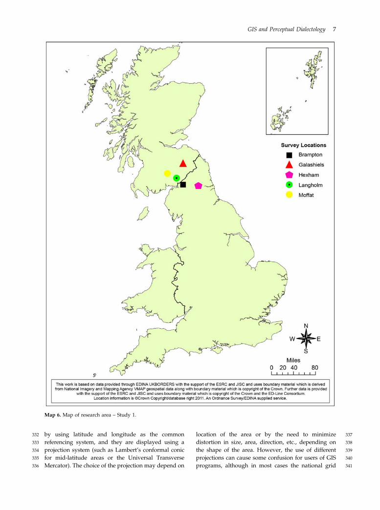
Map 6. Map of research area – Study 1.


342 projection of the users’ home country should be used343 in georeferencing. We discuss georeferencing in rela-344 tion to PD data in more detail below.345 Once data has been georeferenced, a GIS offers346 many possibilities for advanced data processing347 (known as ‘‘geoprocessing’’). Many geoprocessing tools348 are designed for commercial or environmental ends,349 although they can also be used for other purposes such350 as working with linguistic data. In addition to various351 possibilities offered by geoprocessing tools, a GIS also352 provides different ways of visualizing data or creating353 maps. Thus, maps are georeferenced and therefore354 spatially meaningful, unlike conventional maps which355 contain only visual information (i.e. they consist of pixels356 of different colors). Moreover, all geographical data can357 have or be linked to many different types of attributes358 (metrical, numerical, descriptive, complex; cf. Gomarasca,359 2009:484).360 In summary, a GIS enables a user to process,361 analyze, and visualize all kinds of models of the362 earth’s surface. This makes the technology attractive363 not only for geographers and geologists, but also for364 researchers of other disciplines (like archeology,365 forestry, architecture, or civil engineering) as well as366 administrative applications (like urban planning or367 traffic control) (Saurer & Behr, 1997:10). In (perceptual)368 dialectology, however, such technology has been used369 very rarely so far (exceptions being Kirk & Kretzsch-370 mar, 1992; Labov et al., 2006; Lameli et al., 2008; Evans,371 2011; Cukor-Avila et al., 2012; Jeon & Cukor-Avila,372 2012). This is despite the fact that dialectological373 questions and problems are by definition related to

374geographical space. Generally speaking, much simpler375technologies have been used to create maps, the aims376of which were not necessarily ‘‘spatially sensitive’’377(Britain, 2009:144).378In dialect production studies, all necessary geogra-379phical information is selected by the researcher in380advance (e.g. the survey locations). Geographical space381then serves as a template (or ‘‘blank canvass’’; Britain,3822009:144) onto which different linguistic features can383be assigned to predefined places. In PD, however,384geographical data do not only serve as background.385They also present the object of study as they are the386data given by the respondents though their completion387of hand-drawn maps. The enormous advantage of GIS388lies in its ability to process, analyze and visualize these389data and to combine them with reference to other390geography-related data such as topography, political391boundaries, population statistics or dialect isoglosses392(cf. section 4.1).

3933.1. How a GIS works with data

394Computers ‘‘require unambiguous instructions on how395to turn data about spatial entities into geographical396representations’’ (Heywood et al., 2006:77), and as a397result a GIS works with data in specific ways.398Understanding the different ways in which a GIS399deals with data from the real world is important if we400wish to use the technology to process data from PD401(Heywood et al., 2006:77).402A GIS works with data in ‘‘layers,’’ overlaying them403in order to produce composite maps. These layers of

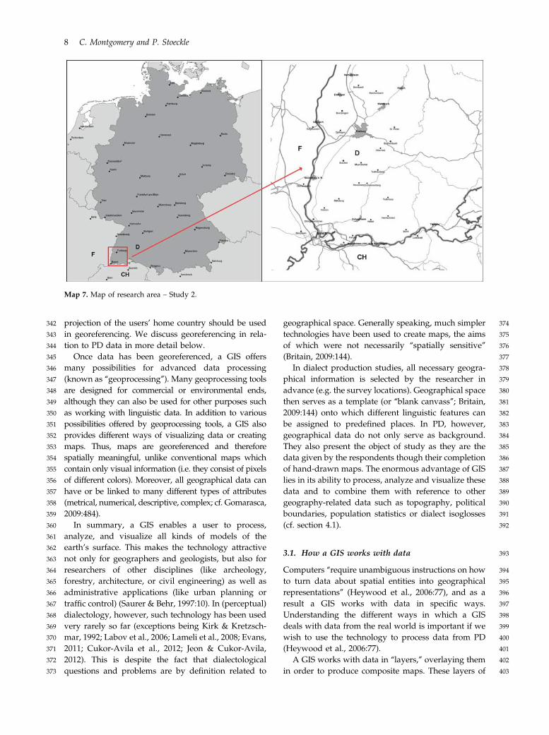
Map 7. Map of research area – Study 2.


404 data can be queried and manipulated, and the405 relationships between them investigated. This makes406 GIS technology particularly attractive for multi-407 layered data such as that gathered in PD research.408 A GIS works with different types of data, and we wish to409 draw readers’ attention to the distinction between the410 two primary types of (spatial) data: raster and vector.

411Raster data can be imagined as a grid, or as412consisting of cells. Each of these cells has a certain413value that is ‘‘mirrored by an equivalent row of414numbers in the file structure’’ (Heywood et al.,4152006:79). A real-world object mapped as a raster will416therefore ‘‘fill’’ some of the cells in the grid, which will417correspond to its shape in the real world. Since every

Figure 1. Vector and raster data (adapted from Heywood et al., 2006:78).


418 pixel – the smallest element that can be visualized—419 has a value, raster datasets can become very large420 regarding storage requirements. In this respect the421 pixel size is also an important factor. While a smaller422 pixel (or cell) size implies a higher resolution of the423 presented surface and may therefore give a more424 detailed view of the phenomena to be dealt with, it425 also leads to a larger file size and slower processing of426 the data. So the choice of the pixel size should always427 depend on the level of detail to be captured from the428 real world. For these reasons, raster datasets are429 especially useful as surface models of small geographic430 areas. Unlike vector datasets, they cannot be connected431 to or contain attribute tables (see below), which limits432 their usefulness if a user wishes to query the data at a433 later stage.434 Vector data use co-ordinates to map real world435 objects, as opposed to the grid and cell method used by436 raster datasets. The file structure of a vector dataset is a437 series of co-ordinate points. These points can be438 connected in order to form lines or polygons. Unlike439 areas in raster datasets there is no information stored440 about surface characteristics (i.e., the individual points441 within an area). Figure 1 shows the different ways in442 which vector and raster data are represented in a GIS.443 Attribute data are a third type of data (Nash Parker444 & Asencio, 2008:xvi), and they are also important for445 GIS processing. This data type provides descriptive

446information linked to the map data by the GIS. It can447contain information about the name of an individual448piece of the map data, for example, but can also449contain a good deal more information about the map450data (such as population size, statistical information,451etc.). We will demonstrate the use of both raster and452vector datasets in this article, along with attribute data,453which assists in querying processed data.

4543.2. General steps involved in processing data from455hand-drawn maps

456The steps involved in processing data from hand-457drawn maps described below do not differ signifi-458cantly from those used by Preston & Howe (1987) or459Onishi & Long (1997). Data relating to dialect areas460still need to be extracted from maps, attribute data461(in the form of demographic information) added, and462the data processed. Only then can aggregate maps of463dialect areas be displayed. The ArcGIS-based method464we detail below follows these steps relatively closely,465although it does not use technology designed specifi-466cally for the task. This means that what we describe467can at first seem daunting; however, the advantage468of using a widely used and available ‘‘off-the-shelf’’469program will be demonstrated as we proceed.470Although a complete account of every data processing471stage will not be possible here for reasons of space, it is

Map 8. Georeferencing and control points.


472 worth noting at this point that the instructions below will473 require some basic familiarity with the ArcGIS environ-474 ment (or the equivalent environment of the GIS you wish475 to use). This cannot be conveyed here, although there are476 several useful resources available online and elsewhere.9

477 We should also emphasize that the benefits of ‘‘picking478 up’’ techniques by using the software should not be479 underestimated.480 As we discuss above, the essential characteristic of a481 GIS is that it enables users to work with data that are482 georeferenced. The first data processing stage is483 therefore to scan all of the hand-drawn maps and to484 add them to an ArcGIS ‘‘project’’ (the term the program485 gives to map documents). Georeferencing can then486 be done using the ‘‘Georeferencing’’ tool by adding487 ‘‘control points.’’ ‘‘Control points’’ are points that have488 been selected on a map that can be aligned with489 known points on another map. This means that if there is490 no information about a map’s coordinate system, it can491 be georeferenced by using existing data (such as borders,492 rivers, etc.) as reference points that can be associated493 with the map with the help of the control points. Map 8494 shows the principle behind georeferencing, in which495 three control points have been identified.10

496The remainder of this section will use data from497Study 2, in order that a clear workflow can be observed.498Map 9 shows a sample of a map from this study that499has been scanned, added to an ArcGIS project, and500then georeferenced.501Once the map is georeferenced, the dialect areas502drawn by the respondents must be digitized. In503ArcGIS this can be managed by creating a polygon504feature class (a vector data type; cf. section 3.2). After505the creation of the polygon feature class, a file is506created which as yet contains no data. Slots for507attribute data can be created during this step, which508will allow the user to input further data (such as509demographic or attitudinal data) at a later stage.510In order to populate the new polygon feature class,511the ‘‘Editor’’ tool is started and the tool ‘‘Create New512Feature’’ used. This permits the dialect area indicated513on the hand drawn map to be entered into the feature514dataset (here named ‘‘Mental Maps’’) by tracing515around it. As we have discussed above, respondents516in both studies were not only asked to draw maps,517but were also requested to label the areas and to518evaluate them according to different aspects (cf.519section 2). GIS offers the possibilities to add any kind

Map 9. Redrawing of mental map.


520 of attributes to the datasets (cf. section 4.1). In the521 case of Study 2, attributes relating to the respondents522 (place of origin, sex, age) and the dialect area (name of523 dialect area, characteristics) were added to the attri-524 bute table. Map 10 shows both the redrawn dialect525 area as well as the table containing different attributes526 relating to it.11

527 The next stage of the processing method is the hand-528 drawn map aggregation. The first step of this process529 involves adding every redrawn area to one dataset530 (using the same process as described above). Map 11531 shows the same dataset as in Map 10, but now containing532 six different polygons (each representing perceptions of533 the same dialect area drawn by six different respondents)534 with their respective attributes in the table.535 Up to this point, the different polygons are stored in536 one dataset and as a result it is not possible to show537 different degrees of agreement, which is one of the538 aims of the method. This can be achieved by a two-539 stage process: First the self-union of the feature class540 containing all the polygons has to be calculated541 (by using the ‘‘Union’’ tool), and then the frequency542 of each of the polygons in the output has to be counted543 (by using the ‘‘Frequency’’ tool) and the output of this

544calculation added to the map. The frequency count of545all the polygons, in this case ranging from one to six,546gives the different degrees of overlap. Map 12 shows a547possible visualization as a result of this process.548Above, we have outlined the steps that will produce a549basic map displaying agreement about the placement550and extent of a dialect area among a group of respon-551dents. Data processing should not stop here, however, as552this type of dataset (i.e. vector data) requires a large553amount of memory space and is thus hard to handle.12

554Second, it is difficult to either merge the dataset with555other kinds of datasets (e.g. more polygons indicating a556dialect area, or neighboring regions) or to perform557further analyses on it. Third, it displays all of the558single values of overlap, which results in too much559influence from single areas and many sharp borders.560Conversion from vector to raster data is therefore561helpful13 as this data format permits processing without562these drawbacks.563The process outlined above requires the use of a564large dataset in order that the benefits become most565apparent. To this end we have used data from Study 2566relating to the so-called ‘‘Kaiserstuhl’’ [literally emperor’s567chair], a small mountain and former volcano very close

Map 10. Redrawn dialect area (red oval) and attributes table.


568 to the French border that is very well known for its569 viticulture. This was the most readily recognized area570 among respondents in Study 2. Of the total of 218571 respondents, ninety-five identified and drew this area.572 Using the same stage of the data processing technique573 as shown in Map 12, Map 13 shows the perceived574 ‘‘Kaiserstuhl’’ dialect area. For comparison, Map 14575 shows a raster-based map of the perception of the same576 area. The different colors indicate different degrees of577 overlap, ranging from one (green) to ninety (red).578 Although containing the same data, the raster579 dataset shown in Map 14 gives a much better580 impression of respondents’ perception of the ‘‘Kaiser-581 stuhl’’ dialect area than that displayed in Map 13.582 The ‘‘Neighbourhood Statistics’’ tool has been used in583 Map 14 in order to smooth the surface of the data,584 which makes any sharp edges between the different585 degrees of overlap disappear.14 A continuous scale has586 been used with contour lines added. The contour lines587 (unlike in topographic maps) do not indicate altitude,588 but degree of overlap.589 The data processing technique described above is590 summarized in the flow chart shown in Figure 2.15

591There is no doubt that, in addition to improving the592processing and display of PD data, the use of GIS has593numerous advantages over the other processing594techniques discussed above. Chief among these is the595ability to make PD data more useable alongside other596datasets. Other advantages include the customization597of aggregate data, the ability to combine individual598areas on the same map, as well as the numerous599possibilities to perform calculations and statistical600analyses on the data.

6014. Merging different datasets on one map

602GIS allows us to examine the impact of many factors603on a much wider scale and in a much more efficient604fashion by permitting us to merge many different605datasets on the same map, as well as enabling606interrogation of these datasets using tools within607the GIS. This ability permits spatially sophisticated608analysis of (perceptual) dialectological data (Britain,6092002:633). There are a vast number of additional610datasets for Great Britain available via various611sources such as data.gov (HM Government, 2011),

Map 11. Several dialect perceptions added to one dataset.


612 Digimap collections (Edina, 2011), OS Open Data613 (Ordnance Survey, 2011) and in the numerous collections614 gathered at census.ac.uk (U.K. Data Archive, 2011).615 Datasets relating to Germany can be found at the616 GeoDatenZentrum (Bundesamt fur Kartographie617 und Geodasie, 2011) or at Geofabrik (2011). Such datasets618 contain georeferenced data relating to a whole host of619 factors, and we will demonstrate some of these below.620 We have already demonstrated merged datasets621 in Maps 12–14. These maps show aggregate perceptual622 dialect areas overlaid onto nonlinguistic datasets (like623 places, streets, political borders, or topography). This624 is of course the least that we would expect of the625 technology. Indeed, some of the visualizations pre-626 sented in the last section (i.e. Map 13 and a simplified627 version of Map 14) can be achieved by using ‘‘regular’’628 vector graphics editors (such as Corel Draw, Adobe629 Illustrator, etc.). However, besides the fact that all630 information contained within such packages is purely631 visual (i.e. pixels of different colors), with no attributes632 associated to the data, another major disadvantage633 is that such data cannot be used for any further634 processing or analyses. Thus, such tools do not move

635us any further past the opportunities offered by636previous or existing data display/processing tools.637This necessitates the use of GIS in order to undertake638Gomarasca’s three different types of data analysis:639‘‘Spatial Data Analysis, [y] Attributes Analysis, [y]640and Integrated Analysis of Spatial Data and Attri-641butes’’ (Gomarasca, 2009:498f).642Aggregate maps produced by perceptual dialectol-643ogists have always been examined alongside other644maps in order to attempt to find correlations. Early645perceptual work in Japan found that physical and646political boundaries were important for respondents647when completing perceptual tasks (Preston, 1993:376;648Grootaers, 1999). Map 15 shows perceptual areas in the649Northern part of England and the Southern part650of Scotland from Study 1 with the Scottish-English651border and English county boundaries superimposed.652Map 16 shows aggregate data from Study 2, with653religious affiliation boundaries superimposed.654Both Map 15 and 16 demonstrate that there is655agreement between ‘‘official’’ boundaries. As discussed656in more detail in Montgomery (forthcoming), the effect657of the Scottish-English border is striking, with almost

Map 12. Map showing different degrees of overlap.


658 no crossing of the border for each perceptual area.659 The ‘‘Cumbria’’ dialect area in the northwest of660 England also fits almost entirely within the modern661 county of Cumbria. The ‘‘Geordie’’ dialect area is less662 respectful of modern county boundaries, although it663 fits well within the boundaries of the older county664 of Northumberland (cf. Llamas, 2000). A similar665 correlation between perceptual data and traditional666 boundaries can also be seen in Map 16. Indeed, in667 the interviews from Study 2, it was a striking668 observation that in Protestant locations many respon-669 dents explicitly referred to the traditional religious670 borders as the main influences on the current dialect671 structure (cf. Stoeckle, 2010, 2012). The ability to672 test qualitative statements such as this in a GIS is

673another factor that should recommend the use of the674technology.675The use of GIS can also allow us to interrogate data676in order to investigate evidence of specific linguistic677phenomena. For example, regional dialect levelling is678said to be having a large impact on linguistic diversity679in Great Britain (Kerswill, 2003). This is underlined by680maps drawn by Kerswill (The Economist, 2011;681Kinchen, 2011) and Trudgill (1999:83). Such maps682predict a future dialect landscape in England typified683by large city-centred dialect areas. As nonlinguists’684perceptions could act as a bellwether for language685change of this type, a comparison between urban686areas and aggregate perceptual data is appropriate.687Map 17 shows this type of comparison.

Map 13. Self-union of hand-drawn maps indicating agreement rates (vector data).


688 Map 17 does appear to demonstrate that urban689 areas were important when completing draw-a-map690 tasks. Despite the predictions made by others (Trud-691 gill, 1999; Kinchen, 2011), these areas have not yet692 been identified by dialectologists (Montgomery, forth-693 coming). The ability to combine PD data with that694 from other sources (be they datasets relating to urban695 areas as in Map 17 or georeferenced linguistic data) is696 important if we are to continue to test theories of697 language change.698 This section has demonstrated the capabilities of a699 GIS in overlaying many different datasets in order to700 answer specific questions about the perception of701 dialect areas, and (in addition) it has underlined the702 possibilities for combining large amounts of data in the703 same place at the same time.

7044.1. Querying and customizing the display of705aggregate data

706As we discussed above, the ability to query the707aggregate dataset was one of the main motivations708for Preston’s shift to a computer-based method of709working with draw-a-map data (Preston & Howe,7101987:369). The advantage of using a computer to711query data and display the result is clear: The712data only need to be entered once. To redraw areas713by hand for each variable the researcher wishes to714examine is neither desirable nor practical. To this715end, query functions were built into both Preston &716Howe’s (1987) method as well as PDQ (Onishi & Long,7171997). PDQ’s query facilities were limited to age,718sex, and informant number (which could then be

F

D

90

...

1

15

30

45

60

75

Freiburg

Waldkirch

Elzach

Endingen

Breisach

Neuenburg a. R.

Herbolzheim

Staufen

Bombach

Neuenweg

Oberried

Opfingen

St. Peter

Buchenbach

Boetzingen

Volgelsheim

Ottmarsheim

Todtnauberg

Muenstertal

Reichenbach

Schoenenberg

Map 14. Rasterized version of hand-drawn maps (with contours).


Figure 2. Workflow for processing draw-a-map data and projecting onto a map in ArcGIS.


719 used for isolating a group of respondents from a720 particular location) (Montgomery, 2007:95). The ability721 to query data entered into a GIS is, on the other hand,722 practically unlimited, dependent only on what an

723attribute table has been set up to contain (step 4 of the724workflow in Figure 2).725The attribute table could contain information726about basic biographical data of the type we might

Map 15. English respondents perceptions of dialect areas and Northern England and Southern Scotland, with national andcounty boundaries superimposed.


727 expect of modern sociolinguistic approaches to speech728 communities (e.g., social variables such as sex, age,729 gender, social network score, etc.). As (perceptual)730 dialectologists are interested in spatiality in addition to731 these factors, other attributes might also be important,732 such as travel history or postcode (ZIP code) informa-733 tion relating to each respondent. We might also be734 interested in those dialect areas characterized as735 ‘‘rough,’’ ‘‘posh,’’ or ‘‘friendly’’ areas (or other labels736 of this sort). Details of all such variables can be added737 to the attribute table and then used to query the data.738 Map 18 shows the result of a query from Study 2 in739 which polygons drawn only by the male and female740 respondents are indicated.741 Querying the datasets in a GIS need not only rely on742 information contained within the attribute table, and it743 is possible to use the geoprocessing tools, which we744 have previously discussed (e.g. for the calculation and745 display of unions, frequencies, and contours, etc.) to746 further interrogate processed data. In a similar fashion,747 GIS programs contain different kinds of measuring

748functions which allow calculations of distances, areas,749and lengths (Gomarasca, 2009:500). Common ques-750tions that perceptual dialectologists may want to ask751are: How large is perceived area A in comparison to752perceived area B? Which people draw the largest dialect753areas? (Cf. Map 18, where female respondents appear754to have drawn larger areas than male respondents);755How big is the distance between a subjective dialect area and756the national border? Of course it is also possible to757combine different types of dialect areas, for example758‘‘subjective’’ and ‘‘objective’’ dialect areas, and examine759where they intersect and how much they overlap.760Although the primary function of PD research is to761examine perceptions of dialect areas through aggregation762of hand-drawn maps, in some contexts it can be763interesting to determine where subjective borders are764particularly stable (cf. Preston, 1986). Map 19 shows a765summary of all dialect areas drawn by the respondents766from Study 2. At first glance the image looks quite767confusing, although it already gives an idea of where768lines occur at a higher frequency.

Map 16. Mental maps from Schopfheim respondents and traditional confessional structuring.


769 For a more sophisticated insight, it is possible to770 calculate the line density of the subjective dialect borders771 using a GIS ‘‘Line Density’’ tool. The result is the raster772 map shown in Map 20 that displays the number of lines773 that occur within a certain research radius for each cell.

774This technique gives a much clearer idea of775where mental borders accumulate. There are certain776correlations that are immediately apparent, most777significantly the coincidence of mental and political778borders.

Map 17. English respondents perceptual areas, with urban areas superimposed.


779 GIS tools also permit the customization of the780 display of aggregate data, something that the techni-781 ques used by Preston & Howe (1987) and Onishi &782 Long (1997) were not able to accomplish. In many783 cases it is useful to show percentages of agreement784 instead of absolute values (cf. Long, 1999; Montgom-785 ery, 2007). This can easily be achieved using raster786 datasets by using interval shading instead of contin-787 uous visualization scales (such as that seen in Map 14).788 Map 21 shows the use of interval shading.789 Map 21 shows the hand drawn maps from the790 ninety-five respondents who drew the ‘‘Kaiserstuhl’’791 dialect area. The interval size to display steps of792 10 percent is therefore 9.5. Of course, PDQ permitted793 such a display of percentage agreement, as demon-794 strated in Map 2. However, what PDQ did not allow795 was the customization of the percentage display, for

796which there were fixed intervals (either 5 or 7 percentage797boundaries). In addition, all of the data are shown on the798composite map. There is no possibility of making some799of the lower agreement level transparent, for example, in800order to present the ‘‘best fit’’ data.801The approach that we describe here enables the user802to control the amount of information presented in803the aggregate map. Percentage agreement levels16 can804be customized, with low levels of agreement made805transparent. Although it is possible for the user to806customize the percentage agreement levels in the GIS807program, most GIS software has in-built methods for808class interval shading (Heywood et al., 2006:258–60).809Such methods include the ‘‘equal interval’’ described in810relation to the percentage agreement levels above, as811well as other techniques including ‘‘nested means’’812and ‘‘natural breaks’’ (Heywood et al., 2006:259).

Map 18. Mental maps drawn by female and male respondents.


813 Solid blocks of color without percentage shading can814 also be created using the equal interval method in815 order to compare PD data with other raster datasets.816 Map 22 demonstrates this functionality, with all exam-817 ples taken from data gathered as part of Study 1818 indicating a Geordie [Newcastle upon Tyne] dialect area.819 That a GIS divides datasets into layers means that it820 is very easy to change the order in which layers appear821 in a map projection. This is especially true when822 the impact of various extra-linguistic (or linguistic)823 factors on subjective dialect perception is considered824 (cf. section 4.0). It is also possible to modify the825 transparency of layers in the GIS in order to examine

826the possible effects of other factors more clearly. In827Map 23, roads, places, and political borders have been828placed on top of the hand-drawn maps, and transpar-829ency has been used. In this way multiple possible830influences, such as the political border between Germany831and France, or topography, become more apparent

8324.2. Combining aggregates of individual areas on833the same map

834Preston (1999a:326) pioneered the approach which saw835the combination of aggregate data for individual dialect836areas on the same map, resulting in maps similar to that

Map 19. Summary of all dialect areas drawn by the respondents from Study 2.


837 shown in Map 24. This approach has generally been used838 to display results from large-scale dialect studies, although839 its utility is also clear for small-scale research projects.840 Such composite maps are helpful as they can be841 compared with other maps indicating boundaries842 arising from production-based studies (see Montgomery,843 2007:242). They also give a useful overview of the844 perception of dialectal variation in a particular country845 (or area of a country). Hitherto, however, they have846 not been straightforward to create. PDQ does not847 easily allow the creation of such maps. Instead, in848 order to compile such a map the researcher must trace849 around the edge of an agreement level for each of the

850aggregate dialect areas. Each of these lines is then851placed back onto a map and labeled manually. This852is a relatively laborious process, and it introduces853another level of potential error into the data. This is854not the largest issue with the technique, but the loss of855the agreement data for each of the areas is a more856substantial problem. This means that for each area,857the map reader is left with outline data only and as858such has no idea where the perceptual ‘‘cores’’ of each859area are to be found, nor where the lowest levels of860agreement can be seen.861The GIS method we advocate here removes the need862to undertake an additional stage of data processing.

F

D

CH

Freiburg

Waldkirch

Weil a. R.

Elzach

Tiengen

opfheim

Endingen

Breisach

Neuenburg a. R.

Bad SaeckingenRheinfelden (CH)

Herbolzheim

Buch

Hasel

Herten

Holzen

Karsau

Staufen

Bombach

Malsburg Todtmoos

Neuenweg

Oberried

Opfingen

Leibstadt

Blotzheim

St. Peter

Buchenbach

Boetzingen

Volgelsheim

Ottmarsheim

Todtnauberg

Muenstertal

Reichenbach

Herrischried

Schoenenberg

Efringen-KirchenSch

Map 20. Line density of mental dialect borders.


863 Instead the GIS can work with all of the aggregate864 areas together in one map. Map 25 shows the type of865 map that can be achieved using this method.866 The resulting composite map loses none of the867 agreement data, while also permitting the display of868 overlapping dialect areas. In addition, the raster data869 generated using the method described here can be870 displayed alongside data held in a vector model, such871 as roads, political boundaries and other linear data.

872 5. Summary: the benefits of the use of GIS873 for PD study

874 The ability to offer improved visualization quality, to875 customize aggregate data, to combine individual areas876 on the same map, and to perform calculations and

877statistical analyses are all steps forward in the878processing and aggregation of PD data. The use of879GIS improves the quality of visualization tools avail-880able to researchers. This is a persuasive reason for881us to move toward the wholesale adoption of the882technology, although the way in which a GIS can work883with data presents an even more appealing proposi-884tion. Thus, the ability to use the functionality of GIS885technology to make PD data more comparable with886that from elsewhere, as well as to subject them to all887kinds of geoprocessing makes the case for using GIS888very strong.889We hope to have demonstrated above that the use of890GIS for processing PD data can result in a good many891benefits. Although the processing techniques can be892labor intensive and time consuming, they are no more

F

D

1-10 %

11-20 %

21-30 %

31-40 %

41-50 %

51-60 %

61-70 %

71-80 %

81-90 %

91-100 %

Freiburg

Waldkirch

Elzach

Endingen

Breisach

Neuenburg a. R.

Herbolzheim

Staufen

Bombach

Neuenweg

Oberried

Opfingen

St. Peter

Buchenbach

Boetzingen

Volgelsheim

Ottmarsheim

Todtnauberg

Muenstertal

Reichenbach

Schoenenberg

Map 21. Rasterised version of hand-drawn maps displaying percentages.


893 so than the alternatives that have been used in the past894 (such as Onishi & Long, 1997). The time and effort895 spent processing data in a GIS is also not to be seen as896 an end in itself, as we have mentioned above. The897 ability to display PD data in a more readily accessible

898and visually more appealing manner is not the main899benefit of the approach we outline in this article.900Instead, the huge possibilities of working with PD901data in a truly ‘‘spatially sensitive’’ (Britain, 2009:144)902fashion should open up the use of this technology to

Map 22. Differences in map display as a result of customizing aggregate data display.


903 others in the fields of dialectology and sociolinguistics.904 We urge that GIS be seen as an exciting new tool that905 can be used to integrate and interrogate data. In this906 way we echo van Hout (in Nerbonne et al., 2008), who907 has stated that this type of approach ‘‘opens up new908 vistas for doing research’’ by giving us ‘‘opportunities909 to open up, combine and integrate various rich data910 sources (e.g. historical, geographical, social, political,911 linguistic), again and again’’ (van Hout in Nerbonne912 et al., 2008:25).913 The processes we have detailed above mean that914 the datasets created within the GIS are useable in a915 widely supported format, permitting further use of them916 by other interested parties. The use of georeferenced917 datasets in other areas of geolinguistics (Lameli et al.,

9182010) means that similarly referenced datasets from PD919research can be used in conjunction with these data in920order to further query data we already know well.921In addition to this, the processing techniques we outline922here mean that we can move beyond the static923representation of perceptions of dialect areas, and instead924use the tools present within GIS programs to perform925sophisticated analyses on the data. This was always the926aim of Long, who adapted parts of the PDQ program to927do just this (see Long, 1997), and continuing along this928path should make the use of GIS essential for accessing929some of the hitherto ‘‘hidden’’ aspects of PD data.930Other visualization possibilities should also not be931neglected, and it seems that the ability to produce 3D932animation in order to further explore PD data

F

D

1-10 %

11-20 %

21-30 %

31-40 %

41-50 %

51-60 %

61-70 %

71-80 %

81-90 %

91-100 %

Freiburg

Waldkirch

Elzach

Endingen

Breisach

Neuenburg a. R.

Herbolzheim

Staufen

Bombach

Neuenweg

Oberried

Opfingen

St. Peter

Buchenbach

Boetzingen

Volgelsheim

Ottmarsheim

Todtnauberg

Muenstertal

Reichenbach

Schoenenberg

Map 23. Transparent rasterised version of hand-drawn maps.


933 (see Animation 1) might have its uses. The production934 of change-over-time animations, which the use of GIS935 can facilitate, is also of clear benefit to sociolinguists936 and dialect geographers, as well as those involved in937 PD study, who wish to examine such phenomena in938 their data.

939 5.1. Possibilities of GIS for general linguistic study

940 Having demonstrated some of the advantages of941 GIS for PD research, we do not think that this is all942 that can be said about this technology. Although943 the possibilities offered by GIS may be essential for944 processing and analyzing hand-drawn map data, there945 are also many benefits for other types of linguistic946 research. Many of the questions and research referring to947 the relationship between language and space (cf. Auer &948 Schmidt, 2010; Lameli et al., 2010) could profit from the949 opportunities outlined in this paper.950 Among their observations concerning the digitiza-951 tion of language mapping, Kehrein et al. state that952 mappings of linguistic data often are ‘‘subject to all953 kinds of limitations’’ (2010:xvii); that is, large parts of

954the data are not displayed and thus not accessible for955other linguists. The use of GIS could contribute to956overcoming this lack of information, since the out-957comes of linguistic studies could be presented as958datasets (cf. section 5.3) rather than just as images.959Even more important seems to be another aspect960which Kehrein et al. observe: ‘‘Linguistic maps are961often difficult to compare because they all use their962own (idiosyncratic) symbolization, map projection,963scale, etc.’’ (2010:xvii). In a GIS, all of these factors964can be handled freely, which would enhance the965comparability of different data.

9665.2. Use of the technology: future directions

967This article has focussed on PD data and the benefits of968working with it in a GIS. However, we do not wish to969claim that this is the only area of sociolinguistic970investigation that can benefit from the use of the971technology. Scholars working in neighboring disci-972plines, such as those who deal with questions about973language and space, can also benefit greatly from the974use of GIS. Georeferenced data is all that is needed for

Map 24. Composite perceptual map of England (Montgomery, 2007:237).


975 such scholars to start using the technology, and all that976 is required for this is the collection of postcode/ZIP977 code data. Once such data is captured, results of these978 studies can be worked within a GIS. In order for data979 from linguistic investigations (PD or otherwise) to be980 truly useful for those in other fields, gathering accurate981 metadata is essential. Metadata documents how spatial982 information has been captured and stored, which is983 important, since when data is captured and stored in984 digital form it is seldom questioned by later users (which985 means that metadata must be accurate and fulsome in986 order that later users do not compare ‘‘apples and987 oranges’’). Accurate and complete metadata is therefore988 vital if linguists wish to add to the body of spatial data.989 In PD, however, the use of this technology is not990 only helpful but instead it seems vital. Not only does it991 improve the quality of visualization of data, but it also992 permits spatial analyses of linguistic data that would993 not be possible with other types of computer software.994 Besides the gains that could be made in PD research,995 more extensive use of GIS by a greater number of996 linguists would lead to a good deal of progress in

997many respects. Comparable to other databases [such as998the ‘‘Archiv fur Gesprochenes Deutsch’’ [Archive for999spoken German] (Institut fur Deutsche Sprache, 2011),

1000the Digital Wenker atlas (Lameli et al., 2010), and the1001Linguistic Atlas Projects web pages (Kretzschmar,10022005)], data and outcomes from studies in PD could1003be available for other linguists. As we have argued,1004they could also be compared with and merged very1005easily with other datasets, be they linguistic or1006nonlinguistic. Moreover, like any other kinds of1007statistical data published on the web (e.g. population1008density, demographic factors, education, etc.) linguis-1009tic data could make up databases available for other1010linguists, but also accessible for the interested public1011(cf. Lameli et al., 2010; Evans, 2011).1012As GIS is used in many fields, it is subject to1013constant development and improvement. More users1014dealing with linguistic topics would promote academic1015exchange and lead to more ideas, more forums, and1016more progress in answering questions related to1017language and space. Kehrein et al. predict that the1018connection between linguistics and GIS ‘‘will be of

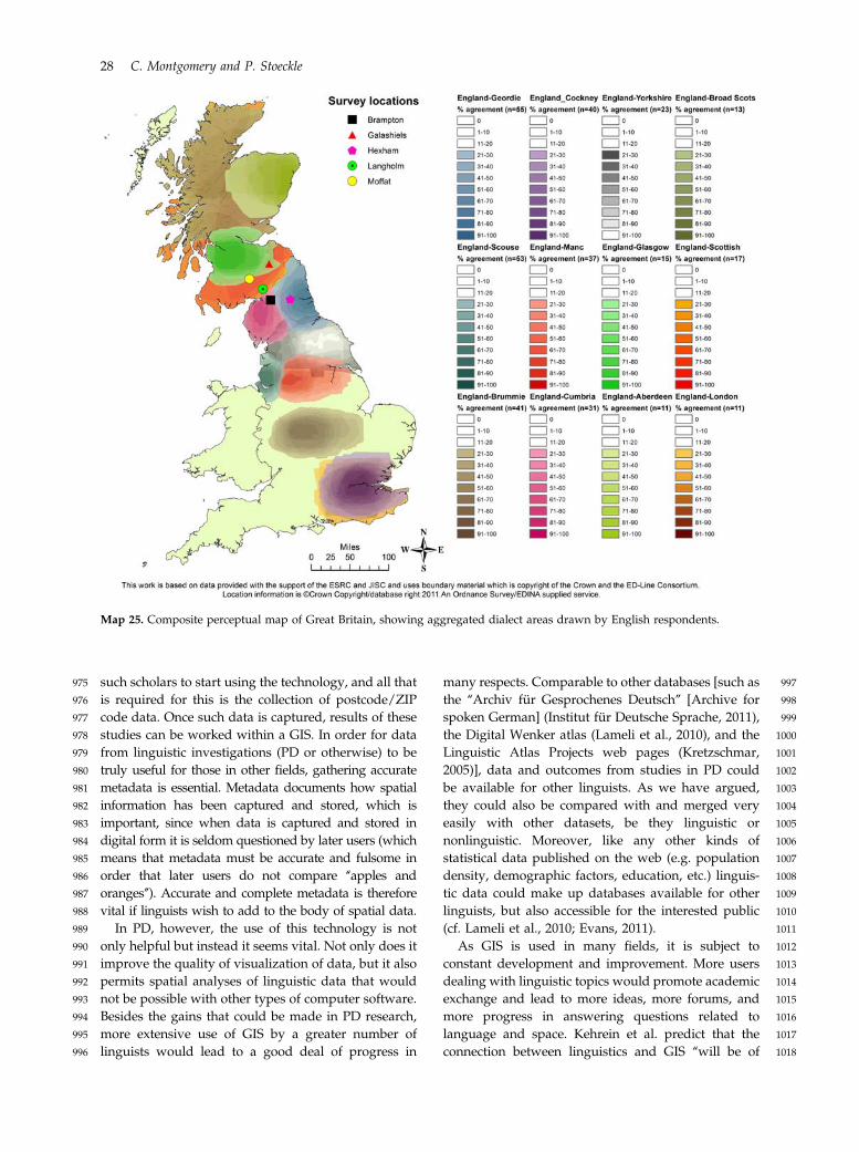
Map 25. Composite perceptual map of Great Britain, showing aggregated dialect areas drawn by English respondents.


1019 increasing importance in the coming years’’ (2010:xviii).1020 We hope to have established some of the most important1021 uses of GIS in PD and delivered some of the decisive1022 arguments for the use of GIS.

1023 Notes

1024 1 Trace-and-overlay techniques can be useful for ‘‘quick and1025 dirty’’ analyses, and should not be dismissed out of hand1026 as they can be instructive as to the general patterning of1027 perceptual areas. In such a technique, lines are compiled1028 using an overhead transparency onto which can be traced1029 all instances of a particular dialect area. The same can be1030 done by scanning maps and manually overlaying them in1031 a graphics program. Producing very detailed composite1032 maps using this type of technique is, however, almost1033 impossible, as is working with data from more than a1034 limited sample (around thirty respondents). Therefore, a1035 trace-and-overlay technique should only be used for1036 small-scale or preliminary studies, or where the aim is to1037 find broad general patterns from a limited cohort.

1038 2 The research in Study 1 was funded by the Economic and1039 Social Research Council, Grant number PTA-026-27-1956.

1040 3 The survey was part of a larger project called ‘‘Regional1041 Dialects in the Alemannic Border Triangle’’ (together with1042 Sandra Hansen). The investigation aims at analysing1043 dialectal variation from both linguistic and folk perspec-1044 tives and to combine the outcomes of the two approaches.

1045 4 The question of how different types of information (such as1046 cities, rivers, administrative boundaries, etc.) may influ-1047 ence the outcome of the draw-a-map task is addressed by1048 Lameli et al. (2008) and shall not be discussed here. In this

1049case, the decision to include the city location dots was1050made to ensure that respondents’ geographical knowl-1051edge was consistent and the spatial data they provided1052could be treated as accurate (cf. Preston, 1993:335).1053Further details relating to this methodological decision1054can be found in Montgomery (2007).

10555 This question was included in order to increase the like-1056lihood of respondents completing the draw-a-map task.1057As Montgomery (2007:71–73) has discussed elsewhere, the1058inclusion of such dots increases the number of respondents1059willing to draw lines on the map, as it reduces the chance of1060getting the geography of the country ‘‘wrong.’’

10616 A question relating to the ‘‘north-south’’ divide was inclu-1062ded as it is an important concept in the United Kingdom1063(although it is perhaps of most importance in England).1064Barely a month goes by without media outlets reporting1065on the existence of the divide (or its ‘‘widening’’1066or ‘‘shrinking’’) (e.g. Wachman, 2011). In this sense, the1067concept is convenient shorthand for a complex situation.1068Although often thought of as a modern or recent concept,1069Jewell has stated that it is ‘‘literally, as old as the hills’’1070(Jewell, 1994:28). The preoccupation with a countrywide1071‘‘divide’’ is perhaps not as surprising as one might think, as1072implicit or explicit contrasts have been shown to be impor-1073tant in creating a sense of ‘‘social self’’ (Cohen, 1985:115).1074Despite this, the divide is not an official boundary and, as1075such, there is a great deal of disagreement about where the1076dividing line falls (Montgomery, 2007:1–4). This question1077was included for the reason that the north-south divide1078is: (a) consistently mentioned, (b) a persistent concept,1079(c) potentially important for a sense of ‘‘social self,’’ and1080(d) undefined.

Animation 1. Fly-over of a 3D representation of North-South dividing lines drawn by respondents from English locations inStudy 1.


1081 7 All interviews were attended by at least one of the1082 researchers, which made it possible to resolve confusions1083 concerning the task immediately.

1084 8 There are various other pieces of GIS software, such as1085 MapInfo (MapInfo Corporation, 2011). Some GIS platforms1086 have a free license [such as Quantum GIS (QGIS, 2011) and1087 GRASS GIS (GRASS Development Team, 2011)].

1088 9 General introductions to GIS can be found in Gomarasca1089 (2009) or Wise (2002). Moreover, there are individual1090 information sites and tutorials for different GIS software1091 providers (such as ESRI, 2011a; GRASS Development1092 Team, 2011; QGIS, 2011).1093 10 It should be noted that three control points are the mini-1094 mum required to georeference an image. More can be1095 used in order to improve accuracy and best practice dic-1096 tates that four or more control points should be used in1097 digitizing or georeferencing. Ideally numerous control1098 points spread out within the area of interest should be1099 identified using discrete (unambiguous) locations (such as1100 borders).1101 11 It is worth noting here that the red coloring of the area is1102 totally at random and that the visualization, as will be1103 shown in section 4.2, can be performed at will.1104 12 This is especially true if many nodes—as in our case,1105 where large numbers of polygons are combined in one1106 dataset – are digitized. Simple vector datasets containing1107 few nodes, however, require less memory than compar-1108 able raster datasets.1109 13 If following this process, make sure to use the frequency1110 count given by the use of the ‘‘Frequency’’ tool as the1111 value field for the raster.1112 14 It has to be mentioned here that all modifications should1113 be carried out thoughtfully. While smoothing the sharp1114 edges makes the map ‘‘cleaner’’ looking, this technique1115 can also distort the data.1116 15 It should be noted that this is not the only way of1117 producing aggregate maps in GIS. For example, it is1118 also possible to convert each single hand-drawn map1119 into a raster dataset and then calculate the sum of all1120 datasets. Since with this method data queries are1121 much more laborious (step 7/8), we follow the scheme1122 presented here.1123 16 Known as ‘‘choroplethic’’ values in the GIS literature, but1124 termed ‘‘percentages’’ here because of the familiarity of1125 this concept in sociolinguistics.

1126 References

1127 Anders, Christina A. 2010. Wahrnehmungsdialektologie: Das1128 Obersachsische im Alltagsverstandnis von Laien. Berlin: De1129 Gruyter Mouton.1130 Auer, Peter & Jurgen E. Schmidt. 2010. Language and space:1131 An international handbook of linguistic variation, vol. 1:1132 Theories and methods. Berlin: De Gruyter Mouton.1133 Britain, David. 2002. Space and spatial diffusion. In1134 J. K. Chambers, P. Trudgill & N. Schilling-Estes (eds),1135 The handbook of language variation and change, 603–637.1136 Oxford: Blackwell.1137 Britain, David. 2009. Language and space: The variationist1138 approach. In P. Auer & J. E. Schmidt (eds), Language and

1139space, an international handbook of linguistic variation, 142–162.1140Berlin: Mouton de Gruyter.1141Britain, David. 2010. Conceptualisations of geographic space1142in linguistics. In A. Lameli, R. Kehrein & S. Rabanus (eds),1143Language and space, an international handbook of linguistic1144variation, vol. 2: Language mapping, 69–97. Berlin: Mouton de1145Gruyter.1146Bucholtz, Mary, Nancy Bermudez, Victor Fung, Lisa Edwards1147& Rosalva Vargas. 2007. Hella nor Cal or totally so Cal?1148The perceptual dialectology of California. Journal of English1149Linguistics 35: 325–352.1150Bucholtz, Mary, Nancy Bermudez, Victor Fung, Rosalva1151Vargas & Lisa Edwards. 2008. The normative North and the1152stigmatized South: Ideology and methodology in the1153perceptual dialectology of California. Journal of English1154Linguistics 36: 62–87.1155Bundesamt fur Kartographie und Geodasie. 2011.1156GeoDatenZentrum. Bundesamt fur Kartographie und1157Geodasie. http://www.bkg.bund.de/ (6 November, 2011).1158Butters, Ronald R. 1991. Dennis Preston, perceptual1159dialectology. Language in Society 20: 294–299.1160Cohen, Anthony. 1985. The symbolic construction of community.1161London: Routledge.1162Cukor-Avila, Patricia, Lisa Jeon, Patrıcia C. Rector,1163Chetan Tiwari & Zak Shelton. 2012. Texas – It’s1164like a whole nuther country: Mapping Texans’1165perceptions of dialect variation in the Lone Star state.1166In Proceedings from the Twentieth Annual Symposium1167about Language and Society, Austin, TX: Texas Linguistics1168Forum.1169Edina. 2011. Digimap collections. http://edina.ac.uk/1170digimap/ (28 September, 2011).1171ESRI. 2011a. ArcGIS Resource Center. http://resources.arcgis.1172com/content/web-based-help (10 November, 2011).1173ESRI. 2011b. What is GIS? GIS.com. http://www.gis.com/1174content/what-gis (12 October, 2011).1175Evans, Betsy E. 2011. Seattle to Spokane: Mapping English in1176Washington state. http://depts.washington.edu/folkling/.1177(12 October, 2011).1178Garrett, Peter. 2010. Attitudes to language. Cambridge:1179Cambridge University Press.1180Geofabrik. 2011. Geofabrik. www.geofabrik.de (2 July, 2012).1181Gomarasca, Marion A. 2009. Basics of geomatics. London1182and New York: Springer Dordrecht Heidelberg.1183Goodey, Brian. 1971. City scene: An exploration into the image1184of central Birmingham as seen by area residents. Birmingham:1185Centre for Urban and Regional Studies, University of1186Birmingham.1187Gould, Peter & Rodney White. 1986. Mental maps, 2nd edn.1188Boston: Allen & Unwin.1189GRASS Development Team. 2011. GRASS GIS. http://grass.1190osgeo.org/ (12 October, 2011).1191Grootaers, Willem A. 1999. The discussion surrounding the1192subjective boundaries of dialects. In D. R. Preston (ed.),1193Handbook of perceptual dialectology 1: 115–129. Amsterdam:1194John Benjamins.1195Heywood, Ian, Sarah Cornelius & Steve Carver. 2006.1196An introduction to geographical information systems, 3rd edn.1197Harlow, UK: Pearson Prentice Hall.


1198 HM Government. 2011. Opening up government. http://data.1199 gov.uk/ (28 September, 2011).1200 Institut fur Deutsche Sprache. 2011. Archiv fur Gesprochenes1201 Deutsch. http://agd.ids-mannheim.de/ (6 November, 2011).1202 Jeon, Lisa & Patricia Cukor-Avila. 2012. Urbanicity and1203 language variation and change: Mapping dialect1204 perceptions in and of Seoul. Sociolinguistic Symposium 19,1205 Berlin, Germany.1206 Jewell, Helen M. 1994. The north-south divide: The origins of1207 northern consciousness in England. Manchester: Manchester1208 University Press.1209 Kehrein, Roland, Lameli Alfred & Rabanus Stefan. 2011.1210 Introduction, xi–xvii. In A. Lameli, R. Kehrein & S. Rabanus1211 (eds), Language and Space – An International Handbook of1212 Linguistic Variation, Volume 2: Language Mapping. Berlin:1213 Mouton de Gruyter.1214 Kerswill, Paul. 2003. Dialect levelling and geographical1215 diffusion in British English. In D. Britain & J. Cheshire1216 (eds), Social dialectology: In honour of Peter Trudgill, 223–243.1217 Amsterdam: John Benjamins.1218 Kinchen, Rosie. 2011. Howay! Youths adopt hip accents.1219 The Sunday Times, p. 11.1220 Kirk, John M. & William A. Kretzschmar. 1992. Interactive1221 linguistic mapping of dialect features. Literary and Linguistic1222 Computing 7: 168–175.1223 Kretzschmar, William A. 1999. Preface. In D. R. Preston (ed.),1224 Handbook of perceptual dialectology 1: xvii–xviii. Amsterdam:1225 John Benjamins.1226 Kretzschmar, William A. 2005. Linguistic atlas projects. http://1227 us.english.uga.edu/cgi-bin/lapsite.fcgi/ (10August, 2011).1228 Labov, William, Sharon Ash & Charles Boberg. 2006.1229 The atlas of North American English: Phonetics, phonology, and1230 sound change: A multimedia reference tool. Berlin: Walter de1231 Gruyter.1232 Lameli, Alfred, Tanja Giessler, Roland Kehrein, Alexandra1233 Lenz, Karl-Heinz Muller, Jost Nickel, Christoph Purschke &1234 Stefan Rabanus. 2010. DiWA. Digital Wenker Atlas. http://1235 www.diwa.info/ (10 August, 2011).1236 Lameli, Alfred, Roland Kehrein & Stefan Rabanus. 2010.1237 Language and space, an international handbook of linguistic1238 variation, vol. 2: Language mapping. Berlin: De Gruyter1239 Mouton.1240 Lameli, Alfred, Christoph Purschke & Roland Kehrein. 2008.1241 Stimulus und Kognition. Zur Aktivierung mentaler1242 Raumbilder. Linguistik Online 35(3): 55–86.1243 Llamas, Carmen. 2000. Middlesbrough English: Convergent1244 and divergent trends in a ‘‘part of Britain with no identity’’.1245 Leeds Working Papers in Linguistics and Phonetics 8: 123–148.1246 Long, Daniel. 1997. The perception of ‘‘standard’’ as the1247 speech variety of a specific region: Computer-produced1248 maps of perceptual dialect regions. In Thomas, A. R. (ed.),1249 Issues and methods in dialectology, 256–270. Bangor:1250 University of Wales Press.1251 Long, Daniel. 1999. Geographical perception of Japanese1252 dialect regions. In D. R. Preston (ed.), Handbook of perceptual1253 dialectology 1: 177–198. Amsterdam: John Benjamins.1254 Lynch, Kevin. 1960. The image of the city. Cambridge, MA: MIT1255 Press.1256 MapInfo Corporation. 2011. MapInfo. http://www.mapinfo.1257 com/ (12 October, 2011).

1258Mase, Yoshio. 1999. Dialect consciousness and dialect1259divisions: Examples in the Nagano-Gifu boundary region.1260In D. R. Preston (ed.), Handbook of perceptual dialectology12611: 71–99. Amsterdam: Benjamins.1262McKinnie, Meghan & Jennifer Dailey-O’Cain. 2002. A1263perceptual dialectology of Anglophone Canada from the1264perspective of young Albertans and Ontarians. In D. Long1265& D. R. Preston (eds), Handbook of perceptual dialectology 2:1266277–294. Amsterdam: John Benjamins.1267Montgomery, Chris. 2007. Northern English dialects:1268A perceptual approach. Sheffield: University of Sheffield1269dissertation.1270Montgomery, Chris. 2011. Perceptual dialectology, bespoke1271methods and the future for data processing. 8th United1272Kingdom Language Variation and Change Conference1273(UKLVC8), Edge Hill University.1274Montgomery, Chris. 2012. The effect of proximity in perceptual1275dialectology. Journal of Sociolinguistics 16(5): 638–668.1276Nash Parker, Robert & Emily K. Asencio. 2008. GIS and spatial1277analysis for the social sciences: Coding, mapping and modelling.1278London: Routledge.1279Nerbonne, John, Paul Heggarty, Roeland van Hout & David1280Robey. 2008. Panel discussion on computing and the1281humanities. In J. Nerbonne, C. Gooskens, S. Kurschner &1282R. van Bezooijen (eds), International journal of humanities and1283arts computing, special issue on computing and language variation.12842: 243–259. Edinburgh: Edinburgh University Press.1285Onishi, Isao & Daniel Long. 1997. Perceptual dialectology1286quantifier (PDQ) for Windows. http://nihongo.hum.1287tmu.ac.jp/,long/maps/perceptmaps.htm (2 July, 2012).1288Ordnance Survey. 2011. OS open data. http://1289www.ordnancesurvey.co.uk/oswebsite/products/1290os-opendata.html (28 September, 2011).1291Orleans, Peter. 1967. Differential cognition of urban residents:1292Effects of social scale on mapping. In J. G. Truxal (ed.),1293Science, engineering, and the city, 103–117. Washington, DC:1294National Academy of Sciences.1295Preston, Dennis R. 1982. Perceptual dialectology: Mental1296maps of United States dialects from a Hawaiian1297perspective. Hawaii Working Papers in Linguistics 14: 5–49.1298Preston, Dennis R. 1986. Five visions of America. Language in1299Society 15: 221–240.1300Preston, Dennis R. 1988. Change in the perception of language1301varieties. In J. Fisiak (ed.), Historical dialectology: Regional and1302social, 475–504. Berlin: Mouton de Gruyter.1303Preston, Dennis R. 1993. Folk dialectology. In D. R. Preston1304(ed.), American dialect research, 333–377. Amsterdam: John1305Benjamins.1306Preston, Dennis R. 1999a. A language attitude approach to the1307perception of regional variety. In D. R. Preston (ed.),1308Handbook of perceptual dialectology 1: 359–375. Amsterdam:1309John Benjamins.1310Preston, Dennis R. 1999b. Introduction. In D. R. Preston (ed.),1311Handbook of perceptual dialectology 1: xxiii–xxxix.1312Amsterdam: John Benjamins.1313Preston, Dennis R. 2010. Perceptual dialectology in the 21st1314century. In C. A Anders, M. Hundt & A. Lasch (eds),1315Perceptual dialectology. Neue Wege der Dialektologie (Linguistik –1316Impulse & Tendenzen), 1–30. Berlin: Mouton de Gruyter.


1317 Preston, Dennis R & George M Howe. 1987. Computerized1318 studies of mental dialect maps. In K. M. Denning, S.1319 Inkelas, F. McNair-Knox & J. Rickford (eds), Variation in1320 language: NWAV-XV at Stanford (Proceedings of the Fifteenth1321 Annual Conference on New Ways of Analyzing Variation).1322 361–378. Stanford, CA: Department of Linguistics, Stanford1323 University.1324 Purschke, Christoph. 2011. Regional linguistic knowledge and1325 perception: On the conceptualization of Hessian.1326 Dialectologia 2, Special Issue, 91–118.1327 QGIS. 2011. Quantum GIS: Welcome to the Quantum GIS1328 project. http://www.qgis.org/ (12 October, 2011).1329 Saurer, Helmut & Franz-Joseph Behr. 1997. Geographische1330 Informationssysteme. Eine Einfuhrung, Darmstadt:1331 Wissenschaftliche Buchgesellschaft.1332 Sibata, Takesi. 1999. Consciousness of dialect boundaries.1333 In D. R. Preston (ed.), Handbook of perceptual dialectology 1:1334 39–63. Amsterdam: John Benjamins.1335 Stoeckle, Philipp. 2010. Subjektive Dialektgrenzen im1336 Alemannischen Dreilandereck. In C. A. Anders, M. Hundt1337 & A. Lasch (eds), Perceptual dialectology – Neue Wege der1338 Dialektologie, 291–315. Berlin: Mouton de Gruyter.1339 Stoeckle, Philipp. 2011. The constitution of subjective dialect1340 areas: Towards a hierarchisation of lay classification1341 strategies. 6th International Conference on Language Variation1342 in Europe, Freiburg, Germany.

1343Stoeckle, Philipp. 2012. The folk-linguistic construction1344of local dialect areas – linguistic and extra-linguistic factors.1345In S. Hansen, C. Schwarz, P. Stoeckle & T. Streck (eds),1346Dialectological and folk dialectological concepts of space.1347Current methods and perspectives in sociolinguistic1348research on dialect change, 142–163, 271–275. Berlin:1349Mouton de Gruyter.1350The Economist. 2011. England’s regional accents: Geordie’s1351still alreet. http://www.economist.com/node/187750291352(7 September, 2011).1353Trudgill, Peter. 1999. The dialects of England, 2nd edn. Oxford:1354Blackwell.1355U.K. Data Archive. 2011. Census.ac.uk. http://1356www.census.ac.uk/ (28 September, 2011).1357Wachman, Richard. 2011. North-South divide widens as1358public sector cuts hit businesses. The Guardian. http://1359www.guardian.co.uk/business/2011/oct/17/north-south-1360divide-widens-cuts (2 July, 2012).1361Weijnen, Antonius A. 1946. De Grenzen Tussen de Oost-1362Noordbrabantse Dialecten Onderin. In A. A. Weijnen,1363M. Renders & J. van Guineken (eds), Oost-Noordbrabantse1364Dialectproblernen, 1–15. Bijdragen en Mededelingen der1365Dialecrencommissie van de Koninkjke Nederlandse1366Akademie van Wetenschappen te Amsterdam VII.1367Amsterdam: Noord-Hollandsche Uitgevers Maatschappij.1368Wise, Stephen. 2002. GIS basics. London: Taylor & Francis.


original research geographic information systems and

Documents