Originally published as:

Martre, P., Wallach, D., Asseng, S., Ewert, F., Jones, J. W., Rötter, R. P., Boote, K.

J., Ruane, A. C., Thorburn, P. J., Cammarano, D., Hatfield, J. L., Rosenzweig, C.,

Aggarwal, P. K., Angulo, C., Basso, B., Bertuzzi, P., Biernath, C., Brisson, N.,

Challinor, A. J., Doltra, J., Gayler, S., Goldberg, R., Grant, R. F., Hooker, J., Hunt,

L. A., Ingwersen, J., Izaurralde, R. C., Kersebaum, K. C., Müller, C., Kumar, S. N.,

Nendel, C., o'Leary, G., Olesen, J. E., Osborne, T. M., Palosuo, T., Priesack, E.,

Ripoche, D., Semenov, M. A., Shcherbak, I., Steduto, P., Stöckle, C. O.,

Stratonovitch, P., Streck, T., Supit, I., Tao, F., Travasso, M., Waha, K., White, J.

W., Wolf, J. (2015): Multimodel ensembles of wheat growth: Many models are better

than one. - Global Change Biology, 21, 2, 911-925

DOI: 10.1111/gcb.12768

Available at http://onlinelibrary.wiley.com

© John Wiley & Sons, Inc.

1

Multimodel ensembles of wheat growth: many models are better than one P I E R RE M A R T R E 1 , 2 , D A N I E L W A L LA C H 3 , S E N T H O L D A S S E NG 4 , F RA N K EWERT 5 , J A M E S

W. J O N E S 4 , R E I M U N D P . R Ö T T E R 6 , K ENN E T H J. BO O T E 4 , A LEX C . R U A N E 7 , P ET ER J.

T H O R B U RN 8 , D A V I D E C A M M A R A N O 4 , J E R R Y L . H A T F I E LD 9 , C YN T H I A RO S EN Z W E IG 7 ,

P R A M O D K. A G G A R W A L 1 0 , C A R L O S A N G U L O 5 , B R U N O B A S S O 1 1 , P A T R I C K B E R TU Z Z I 1 2 ,

C H R I S T I A N B I E R N A T H 1 3 , N A D I N E B R I S S O N 1 4 , 1 5 † , A N D R E W J . C H A L L I N O R 16 , 1 7 , J O R D I

D O L T R A 1 8 , S E BA S T I A N G A Y L E R 1 9 , R I C H I E G O L D B E R G 7 , R O B E R T F . G R A N T 20 , L E E

H EN G 2 1 , J O S H H O O K E R 2 2 , L E S L I E A . H U N T 2 3 , J OA C H I M IN G W E R S E N 2 4 , R OB ER TO C . I Z A U R R A L D E 2 5 , K UR T C H R I S T I A N K E R S E B A UM 26 , C HR I S T O P H M U€ L L E R 2 7 , S O O R A

N A R E S H K U M A R 2 8 , C L A A S N E N D E L 2 6 , G A R R Y O ’ L E A R Y 2 9 , J Ø R G E N E . O L E S E N 30 , T O M

M . O S B O RN E 3 1 , T A RU P A L O S U O 6 , E C K A R T P R I ES A C K 1 3 , D O M I N I Q U E R I P O C H E 1 2 , M I K H A I L A . S E M EN O V 3 2 , I U R I I S H C H E R BA K 1 1 , P A S Q U A L E S T E DU T O 3 3 , C LA U D I O O.

ST Ö C K L E 3 4 , P I E R R E S T R A T O N O V I T C H 32 , T H I L O S T R E C K 2 4 , I WAN S U P I T 35 , F ULU T AO 36 ,

M A R I A T R A V A S S O 3 7 , K A TH A R I N A W A H A 27 , J E F F R E Y W . W H I T E 38 and JOOST WOLF 39

1INRA, UMR1095 Genetics, Diversity and Ecophysiology of Cereals (GDEC), 5 chemin de Beaulieu, F-63 100 Clermont-Ferrand,

France, 2Blaise Pascal University, UMR1095 GDEC, F-63 170 Aubiere, France, 3INRA, UMR1248 Agrosystemes et

Developpement Territorial, F-31 326 Castanet-Tolosan, France, 4Agricultural & Biological Engineering Department, University of

Florida, Gainesville, FL 32611, USA, 5Institute of Crop Science and Resource Conservation, Universität Bonn, D-53 115 Bonn,

Germany, 6Plant Production Research, MTT Agrifood Research Finland, FI-50 100 Mikkeli, Finland, 7National Aeronautics and

Space Administration, Goddard Institute for Space Studies, New York, NY 10025, USA, 8Commonwealth Scientific and Industrial

Research Organization, Ecosystem Sciences, Dutton Park, QLD 4102, Australia, 9National Laboratory for Agriculture and

Environment, Ames, IA 50011, USA, 10Consultative Group on International Agricultural Research, Research Program on Climate

Change, Agriculture and Food Security, International Water Management Institute, New Delhi 110012, India, 11Department of

Geological Sciences and Kellogg Biological Station, Michigan State University, East Lansing, MI 48823, USA, 12INRA, US1116

AgroClim, F-84 914 Avignon, France, 13Institute of Soil Ecology, Helmholtz Zentrum München, German Research Center for

Environmental Health, Neuherberg D-85 764, Germany, 14INRA, UMR0211 Agronomie, F-78 750 Thiverval-Grignon, France, 15AgroParisTech, UMR0211 Agronomie, F-78 750 Thiverval-Grignon, France, 16Institute for Climate and Atmospheric Science,

School of Earth and Environment, University of Leeds, Leeds LS29JT, UK, 17CGIAR-ESSP Program on Climate Change,

Agriculture and Food Security, International Centre for Tropical Agriculture, A.A. 6713 Cali, Colombia, 18Cantabrian

Agricultural Research and Training Centre, 39600 Muriedas, Spain, 19Water & Earth System Science Competence Cluster, c/o

University of Tübingen, D-72 074 Tübingen, Germany, 20Department of Renewable Resources, University of Alberta, Edmonton, AB

T6G 2E3, Canada, 21International Atomic Energy Agency, 1400 Vienna, Austria, 22School of Agriculture, Policy and

Development, University of Reading, RG6 6AR Reading, UK, 23Department of Plant Agriculture, University of Guelph, Guelph,

ON N1G 2W1, Canada, 24Institute of Soil Science and Land Evaluation, Universität Hohenheim, D-70 599 Stuttgart, Germany, 25Department of Geographical Sciences, University of Maryland, College Park, MD 20782, USA, 26Institute of Landscape Systems

Analysis, Leibniz Centre for Agricultural Landscape Research, D-15 374 Müncheberg, Germany, 27Potsdam Institute for Climate

Impact Research, D-14 473 Potsdam, Germany, 28Centre for Environment Science and Climate Resilient Agriculture, Indian

Agricultural Research Institute, New Delhi 110 012, India, 29Department of Primary Industries, Landscape & Water Sciences,

Horsham, Vic., 3400, Australia, 30Department of Agroecology, Aarhus University, 8830 Tjele, Denmark, 31National Centre for

Atmospheric Science, Department of Meteorology, University of Reading, RG6 6BB Reading, UK, 32Computational and Systems

Biology Department, Rothamsted Research, Harpenden, Herts AL5 2JQ, UK, 33Food and Agriculture Organization of the United

Nations, Rome 00153, Italy, 34Biological Systems Engineering, Washington State University, Pullman, WA 99164-6120, USA, 35Earth System Science-Climate Change, Wageningen University, 6700AA Wageningen, The Netherlands, 36Institute of

Geographical Sciences and Natural Resources Research, Chinese Academy of Science, Beijing 100101, China, 37Institute for

Climate and Water, INTA-CIRN, 1712 Castelar, Argentina, 38Arid-Land Agricultural Research Center, USDA, Maricopa, AZ

85138, USA, 39Plant Production Systems, Wageningen University, 6700AA Wageningen, The Netherlands

Correspondence: Pierre Martre, tel. +33 473 624 351,

fax +33 473 624 457, e-mail: pierre.martre@clermont.inra.fr †Dr Nadine Brisson passed away in 2011 while this work was being

carried out.

2

Abstract

Crop models of crop growth are increasingly used to quantify the impact of global changes due to climate or crop

management. Therefore, accuracy of simulation results is a major concern. Studies with ensembles of crop models

can give valuable information about model accuracy and uncertainty, but such studies are difficult to organize and

have only recently begun. We report on the largest ensemble study to date, of 27 wheat models tested in four con-

trasting locations for their accuracy in simulating multiple crop growth and yield variables. The relative error aver-

aged over models was 24–38% for the different end-of-season variables including grain yield (GY) and grain protein

concentration (GPC). There was little relation between error of a model for GY or GPC and error for in-season vari-

ables. Thus, most models did not arrive at accurate simulations of GY and GPC by accurately simulating preceding

growth dynamics. Ensemble simulations, taking either the mean (e-mean) or median (e-median) of simulated values,

gave better estimates than any individual model when all variables were considered. Compared to individual models,

e-median ranked first in simulating measured GY and third in GPC. The error of e-mean and e-median declined

with an increasing number of ensemble members, with little decrease beyond 10 models. We conclude that

multimodel ensembles can be used to create new estimators with improved accuracy and consistency in simulating

growth dynamics. We argue that these results are applicable to other crop species, and hypothesize that they apply

more generally to ecological system models.

Keywords: ecophysiological model, ensemble modeling, model intercomparison, process-based model, uncertainty, wheat

(Triticum aestivum L.)

Received 28 May 2014; revised version received 7 August 2014 and accepted 25 September 2014

Introduction

Global change with increased climatic variability are

projected to strongly impact crop and food produc-

tion, but the magnitude and trajectory of these impacts

remain uncertain (Tubiello et al., 2007). This

uncertainty, together with the increasing demand for

food of a growing world population (Bloom, 2011), has

raised concerns about food security and the need to

develop more sustainable agricultural practices

(Godfray et al., 2010). More confident understanding of

global change impacts is needed to develop effec- tive

adaptation and mitigation strategies (Easterling et al.,

2007). Methodologies to quantify global change

impacts on crop production include statistical models

(Lobell et al., 2011) and process-based crop simulation

models (Porter & Semenov, 2005), which are increas-

ingly used in basic and applied research and to sup-

port decision making at different scales (Challinor et

al., 2009; Ko et al., 2010; Angulo et al., 2013; Rosen-

zweig et al., 2013).

Different crop growth and development processes

are affected by climatic variability via linear or non-

linear relationships resulting in complex and unex-

pected responses (Trewavas, 2006). It has been argued

that such responses can best be captured by process-

based crop simulation models that quantitatively

represent the interaction and feedback responses of

crops to their environments (Porter & Semenov, 2005;

Bertin et al., 2010). Wheat is the most important

staple crop in the world providing over

20% of the calories and proteins in human diet

(FAOSTAT, 2014). It has therefore received much

attention from the crop modeling community and over

40 wheat crop models are in use (White et al., 2011).

These differ in the processes included in the models

and the mechanistic detail used to model individual

processes like evapotranspiration or photo- synthesis.

Therefore, a thorough comparative evalua- tion of

models is essential to understand the reliability of

model simulations and to quantify and reduce the

uncertainty of such simulations (Rötter et al., 2011).

The Wheat Pilot study (Asseng et al., 2013) of the

Agricultural Model Intercomparison and Improvement

Project (AgMIP; Rosenzweig et al., 2013) compared 27

wheat models, the largest ensemble of crop models cre-

ated to date. The models vary greatly in their complex-

ity and in the modeling approaches and equations used

to represent the major physiological processes that

determine crop growth and development and their

responses to environmental factors, see Table S3 in As-

seng et al. (2013).

An initial study (Asseng et al., 2013) analyzed the

variability between crop models in simulating grain

yield (GY) under climate change situations without

specifically investigating multimodel ensemble estima-

tors considering other end-of-season and in-season

variables to better justify their possible application. The

present analysis uses the resulting dataset to study how

the multimodel ensemble average or median can repro-

duce in-season and end-of-season observations. In its

3

simplest and most common form, a multimodel ensem-

ble simulation is produced by averaging the simula-

tions of member models weighted equally (Knutti,

2010). This method has been practiced in climate fore-

casting (Räisänen & Palmer, 2001; Hagedorn et al.,

2005) and in ecological modeling of species distribution

(Grenouillet et al., 2011), and it has been shown that

multimodel ensembles can give better estimates than

any individual model. Such improvement in skill of a

multimodel ensemble may be also applicable to crop

models. Preliminary evidence suggests that the average

of ensembles of simulations is a good estimator of GY

for several crops (Palosuo et al., 2011; Rötter et al., 2012;

Bassu et al., 2014) and possibly even better than the best

individual model across different seasons and sites

(Rötter et al., 2012). However, a detailed quantitative

analysis of the quality of simulators based on crop

model ensembles, compared to individual models is

lacking. By looking at outputs of multiple growth vari-

ables (both in-season and end-of-season), we would get

a broader picture of how ensemble estimators perform

and a better understanding of why they perform well

compared to individual models. It is important there-

fore to consider not only GY but also other growth vari-

variables. If multimodel ensembles are truly more

skillful than the best model in the ensemble, or even

simply better than the average of the models, then using

ensemble medians or means may be a powerful

estimator to evaluating crop response to crop

management and environmental factors.

Model evaluations can give quite different results

depending on the use of the model that is studied. Here,

we investigate the situation where models are applied in

environments for which they have not been specifically

calibrated, which is typically the situation in global

impact studies (Rosenzweig et al., 2014). The model

results were compared to measured data from four

contrasting growing environments. The modeling

groups were provided with weather data, soil

characteristics, soil initial conditions, management, and

flowering and harvest dates for each site. Although only

four locations were tested in the AgMIP Wheat Pilot

study, this limitation is partially compensated for by the

diversity of the sites ranging from high to low yielding,

from short to long season, and irrigated and not

irrigated situations.

Two main approaches to evaluate the accuracy and

uncertainty of the AgMIP wheat model ensemble were

followed. First, we evaluated the range of errors and the

average error of the models for multiple growth

variables, including both in-season and endof- season

variables. Secondly, we evaluated two ensemble-based

models, the mean (e-mean) and the median (e-median)

of the simulated values of the

ensemble members. Finally, we studied how the error

of e-mean and e-median changed with the size of the

ensemble.

Materials and methods

Experimental data

Quality-assessed experimental data from single crops at four

contrasting locations representing diverse agro-ecological

conditions were used. The locations were Wageningen, The

Netherlands (NL; Groot & Verberne, 1991), Balcarce, Argentina

(AR; Travasso et al., 2005), New Delhi, India (IN; Naveen,

1986), and Wongan Hills, Australia (AU; Asseng et al., 1998).

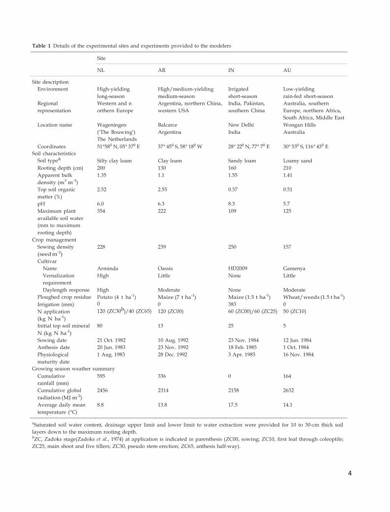
Typical regional crop management was used at each site. In all

experiments, the plots were kept weed-free, and plant

protection methods were used as necessary to minimize

damage from pests and diseases. Crop management and soil

and cultivar information, as given to each individual modeling

group, are given in Table 1.

Daily values of solar radiation, maximum and minimum

temperature, and precipitation were recorded at weather

stations at or near the experimental plots, except for IN solar

radiation which was obtained from the NASA POWER dataset

of modeled data (Stackhouse, 2006) that extends back to 1983.

Daily values of 2-m wind speed (m s-1), dew point temperature

(°C), vapor pressure (hPa), and relative humidity (%) were

estimated for each location from the NASA Modern Era

Retrospective-Analysis for Research and Applications

(Bosilovich et al., 2011), except for NL wind speed and vapor

pressure that were measured on site. Air CO2 concentration

was taken to be 360 ppm at all sites. A weather summary for

each site is shown in Table 1 and Fig. 1.

For all sites, end-of-season (i.e. ripeness-maturity) values for

GY (t DM ha-1), total aboveground biomass (AGBMm, t DM ha-

1), total aboveground nitrogen (AGNm, kg N ha-1), and grain N

(GNm, kg N ha-1) were available. From these values, biomass

harvest index (HI = 100 9 GY/AGBMm, %), N harvest index

(NHI = 100 9 GNm/AGNm, %), and grain protein

concentration (GPC = 0.57 9 GNm/GY, % of grain dry mass)

were calculated. In-season measurements included leaf area

index (LAI, m2 m-2; 15 measurements in total), total

aboveground biomass (AGBM, t DM ha-1; 28 measurements),

total aboveground N (AGN, kg N ha-1; 27 measurements), and

soil water content to maximum rooting depth (mm, 28

measurements). Plant-available soil water to maximum rooting

depth (PASW, mm) was calculated from the measured soil

water content by layer (ΘV, vol%), the estimated lower limit of

water extraction (LL, vol%), and the thickness of the soil layers

(d,m):

𝑃𝐴𝑆𝑊 = ∑ 𝑑𝑖 × (

𝑘

𝑖=1

Θ𝑉,𝑖 − 𝐿𝐿𝑖) (1)

where k is the number of sampled soil layers. Based on the

critical N dilution curve of wheat (Justes et al., 1994), a N

nutrition index (NNI, dimensionless) was calculated to quantify

crop N status. Although this curve is empirical, it is based on

solid theoretical grounds (Lemaire & Gastal,

4

Table 1 Details of the experimental sites and experiments provided to the modelers

Site

NL AR IN AU

Site description Environment High-yielding High/medium-yielding Irrigated Low-yielding

long-season medium-season short-season rain-fed short-season

Regional Western and n Argentina, northern China, India, Pakistan, Australia, southern

representation orthern Europe western USA southern China Europe, northern Africa,

South Africa, Middle East

Location name Wageningen Balcarce New Delhi Wongan Hills

(‘The Bouwing’) Argentina India Australia

The Netherlands Coordinates 51°580 N, 05° 370 E 37° 450 S, 58° 180 W 28° 220 N, 77° 70 E 30° 530 S, 116° 430 E

Soil characteristics

Soil typea Silty clay loam

Clay loam

Sandy loam

Loamy sand

Rooting depth (cm) 200 130 160 210

Apparent bulk 1.35 1.1 1.55 1.41

density (m3 m-3) Top soil organic 2.52 2.55 0.37 0.51

matter (%) pH 6.0 6.3 8.3 5.7

Maximum plant 354 222 109 125

available soil water (mm to maximum rooting depth)

Crop management Sowing density 228 239 250 157

(seed m-2) Cultivar

Name Arminda Oassis HD2009 Gamenya

Vernalization High Little None Little

requirement Daylength response High Moderate None Moderate

Ploughed crop residue Potato (4 t ha-1) Maize (7 t ha-1) Maize (1.5 t ha-1) Wheat/weeds (1.5 t ha-1)

Irrigation (mm)

N application

0

120 (ZC30b)/40 (ZC65)

0

120 (ZC00)

383

60 (ZC00)/60 (ZC25)

0

50 (ZC10)

(kg N ha-1) Initial top soil mineral 80 13 25 5

N (kg N ha-1) Sowing date 21 Oct. 1982 10 Aug. 1992 23 Nov. 1984 12 Jun. 1984

Anthesis date 20 Jun. 1983 23 Nov. 1992 18 Feb. 1985 1 Oct. 1984

Physiological 1 Aug. 1983 28 Dec. 1992 3 Apr. 1985 16 Nov. 1984

maturity date Growing season weather summary

Cumulative 595 336 0 164

rainfall (mm) Cumulative global 2456 2314 2158 2632

radiation (MJ m-2) Average daily mean 8.8 13.8 17.5 14.1

temperature (°C) aSaturated soil water content, drainage upper limit and lower limit to water extraction were provided for 10 to 30-cm thick soil

layers down to the maximum rooting depth. bZC, Zadoks stage(Zadoks et al., 1974) at application is indicated in parenthesis (ZC00, sowing; ZC10, first leaf through coleoptile;

ZC25, main shoot and five tillers; ZC30, pseudo stem erection; ZC65, anthesis half-way).

5

40

(a) The Netherlands

30 Radiation Temperature

Rainfall

Irrigation 20

10

0

40

(b) Argentina m

30 a

20

10

0

40

(c) India m

30 a

20

10

0

40

(d) Australia m

30 a

20

10

0

240

210

a 180 m

150

120

90

60

30

0

210

180

150

120

90

60

30

0

210

180

150

120

90

60

30

0

210

180

150

120

90

60

30

140

120

100

80

60

40

20

0 140

120

100

80

60

40

20

0 140

120

100

80

60

40

20

0 140

120

100

80

60

40

20

0

Models and setup of model intercomparison

The models considered here were the 27 wheat crop models

(Table S1) used in the AgMIP Wheat Pilot study (Asseng et al.,

2013). All of these models have been described in publications

and are currently in use. Not all models simulated all mea-

sured variables, either because the models did not simulate

them or because they were not in the standard outputs. Of the

27 models, 23 models simulated PASW values, and 20 simu-

lated AGN and GN, and therefore NNI and GPC could be cal-

culated for these 20 models. NHI could be calculated for 19

models.

All modeling groups were provided with daily weather

data (i.e. precipitation, minimum and maximum air temper-

ature, mean relative air humidity, dew point temperature,

mean air vapor pressure, global radiation, and mean wind

speed), basic physical characteristics of soil, initial soil water

and N content by layer and crop management infor- mation

(Table S1). No indication of how to interpret or con- vert

this information into parameter values was given to the

modelers. Modelers were provided with observed anthesis

and maturity dates for the cultivars grown at each site.

Qualitative information on vernalization requirements and

daylength responses were also provided. All models were

calibrated for phenology to avoid any confounding effects.

In the simulations, phenology parameters were adjusted to

reproduce the observed anthesis and maturity dates, but

otherwise models were not specifically adjusted to the growth

data, which were only revealed to the modelers at the end of

the simulation phase of the project. The information provided

correspond to the partial model calibration in Asseng et al.

(2013). Modelers were instructed to keep all parameters except

for genotypic coefficients, constant across all four sites. The

soil characteristics and initial conditions and crop manage-

ment were specific to each site but were the same across all

models.

0 50 100 150 200 250 300

Days after sowing

Fig. 1 Weather data at the four studied sites. Mean weekly tem-

perature (solid lines), cumulative weekly solar radiation

(dashed lines), cumulative weekly rainfall (vertical solid bars)

and irrigation (vertical open bars) in (a) Wageningen, The Neth-

erlands, (b) Balcarce, Argentina, (c) New Delhi, India, and (d)

Wongan Hills, Australia. Vertical arrows indicate (a) anthesis

and (m) physiological maturity dates.

1997). Climatic conditions can affect growth and N uptake dif-

ferently, but the NNI reflects these effects in terms of crop N

needs (Lemaire et al., 2008; Gonzalez-Dugo et al., 2010). For a

given AGBM, NNI was calculated as the ratio between the

actual and critical (NC; g N g-1 DM) AGN concentrations

defined by the critical N dilution curve (Justes et al., 1994):

𝑁𝐶 = 5.35 × 𝐴𝐺𝐵𝑀−0.442 (2)

If the NNI value is close to 1 it indicates an optimal crop N

status, a value lower than 1 indicates N deficiency and a value

higher than 1 indicates N excess.

The experimental data used in this study have not been used

to develop or calibrate any of the 27 models. Experi- ments at

AU and NL were used by one and two models as part of

large datasets for model testing in earlier studies, respectively;

but no calibration of the models was done. Except for the

four Expert-N models which were run by the same group,

all models were run by different groups with- out

communication between the groups regarding the

parameterization of the initial conditions or cultivar specific

parameters. In most cases, the model developers ran their

own model.

Model evaluation

Many different measures of the discrepancies between simula-

tions and measurements have been proposed (Bellocchi et al.,

2010; Wallach et al., 2013), and each captures somewhat differ-

ent aspects of model behavior. We concentrated on the root

mean squared error (RMSE) and the root mean squared rela-

tive error (RMSRE), where each error is expressed as a per-

centage of the observed value. The RMSE has the advantage

of expressing error in the same units as the variable. For

Me

an w

ee

kly

tem

ep

era

ture

(°C

)

Cum

ula

ted

sola

r ra

dia

tio

n (

MJ m

–2 w

ee

k–

1)

Rain

fall o

r ir

rig

atio

n (

mm

week–

1)

6

comparing very different environments likely to give a broad

range of crop responses, the relative error may be more

meaningful than the absolute error as it gives more equal weight to

each measurement. However, RMSRE needs to be interpreted with

care because it is very sensitive to errors when measured values

are small, as occurred for several early-season growth

measurements.

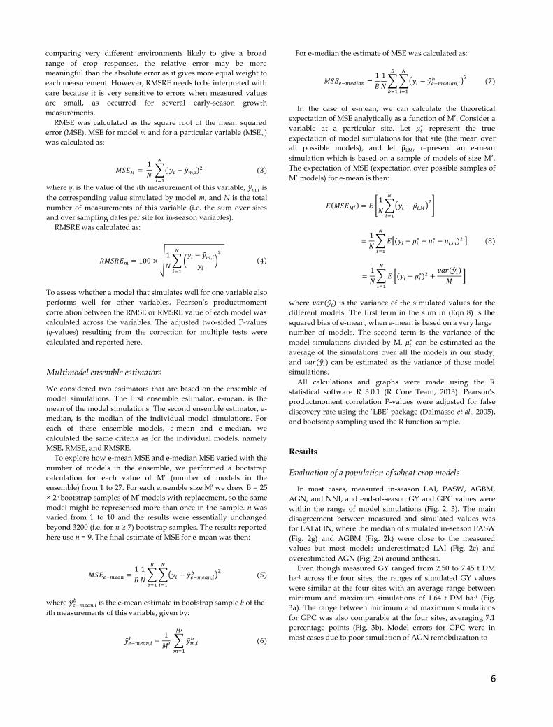
RMSE was calculated as the square root of the mean squared

error (MSE). MSE for model m and for a particular variable (MSEm)

was calculated as:

𝑀𝑆𝐸𝑀 = 1

𝑁 ∑(

𝑁

𝑖=1

𝑦𝑖 − 𝑦𝑚,𝑖)2 (3)

where yi is the value of the ith measurement of this variable, �̂�𝑚,𝑖 is

the corresponding value simulated by model m, and N is the total

number of measurements of this variable (i.e. the sum over sites

and over sampling dates per site for in-season variables).

RMSRE was calculated as:

𝑅𝑀𝑆𝑅𝐸𝑚 = 100 × √1

𝑁∑ (

𝑦𝑖 − �̂�𝑚,𝑖

𝑦𝑖

)2

𝑁

𝑖=1

(4)

To assess whether a model that simulates well for one variable also

performs well for other variables, Pearson’s productmoment

correlation between the RMSE or RMSRE value of each model was

calculated across the variables. The adjusted two-sided P-values

(q-values) resulting from the correction for multiple tests were

calculated and reported here.

Multimodel ensemble estimators

We considered two estimators that are based on the ensemble of

model simulations. The first ensemble estimator, e-mean, is the

mean of the model simulations. The second ensemble estimator, e-

median, is the median of the individual model simulations. For

each of these ensemble models, e-mean and e-median, we

calculated the same criteria as for the individual models, namely

MSE, RMSE, and RMSRE.

To explore how e-mean MSE and e-median MSE varied with the

number of models in the ensemble, we performed a bootstrap

calculation for each value of M’ (number of models in the

ensemble) from 1 to 27. For each ensemble size M’ we drew B = 25

× 2n bootstrap samples of M’ models with replacement, so the same

model might be represented more than once in the sample. n was

varied from 1 to 10 and the results were essentially unchanged

beyond 3200 (i.e. for n ≥ 7) bootstrap samples. The results reported

here use n = 9. The final estimate of MSE for e-mean was then:

𝑀𝑆𝐸𝑒−𝑚𝑒𝑎𝑛 =1

𝐵

1

𝑁∑ ∑(𝑦𝑖 − �̂�𝑒−𝑚𝑒𝑎𝑛,𝑖

𝑏 )2

𝑁

𝑖=1

𝐵

𝑏=1

(5)

where �̂�𝑒−𝑚𝑒𝑎𝑛,𝑖𝑏 is the e-mean estimate in bootstrap sample b of the

ith measurements of this variable, given by:

�̂�𝑒−𝑚𝑒𝑎𝑛,𝑖𝑏 =

1

𝑀′ ∑ �̂�𝑚,𝑖

𝑏

𝑀′

𝑚=1

(6)

For e-median the estimate of MSE was calculated as:

𝑀𝑆𝐸𝑒−𝑚𝑒𝑑𝑖𝑎𝑛 =1

𝐵

1

𝑁∑ ∑(𝑦𝑖 − �̂�𝑒−𝑚𝑒𝑑𝑖𝑎𝑛,𝑖

𝑏 )2

(7)

𝑁

𝑖=1

𝐵

𝑏=1

In the case of e-mean, we can calculate the theoretical

expectation of MSE analytically as a function of M’. Consider a

variable at a particular site. Let 𝜇𝑖∗ represent the true

expectation of model simulations for that site (the mean over

all possible models), and let μ̂i,M′ represent an e-mean

simulation which is based on a sample of models of size M’.

The expectation of MSE (expectation over possible samples of

M’ models) for e-mean is then:

𝐸(𝑀𝑆𝐸𝑀′) = 𝐸 [1

𝑁∑(𝑦𝑖 − �̂�𝑖,𝑀)

2𝑁

𝑖=1

]

=1

𝑁∑ 𝐸[(𝑦𝑖 − 𝜇𝑖

∗ + 𝜇𝑖∗ − 𝜇𝑖,𝑚)2 ]

𝑁

𝑖=1

(8)

=1

𝑁∑ 𝐸 [(𝑦𝑖 − 𝜇𝑖

∗)2 +𝑣𝑎𝑟(�̂�𝑖)

𝑀 ]

𝑁

𝑖=1

where 𝑣𝑎𝑟(�̂�𝑖) is the variance of the simulated values for the

different models. The first term in the sum in (Eqn 8) is the

squared bias of e-mean, when e-mean is based on a very large

number of models. The second term is the variance of the

model simulations divided by M. 𝜇𝑖∗ can be estimated as the

average of the simulations over all the models in our study,

and 𝑣𝑎𝑟(�̂�𝑖) can be estimated as the variance of those model

simulations.

All calculations and graphs were made using the R

statistical software R 3.0.1 (R Core Team, 2013). Pearson’s

productmoment correlation P-values were adjusted for false

discovery rate using the ‘LBE’ package (Dalmasso et al., 2005),

and bootstrap sampling used the R function sample.

Results

Evaluation of a population of wheat crop models

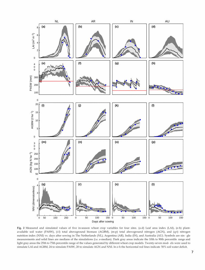
In most cases, measured in-season LAI, PASW, AGBM,

AGN, and NNI, and end-of-season GY and GPC values were

within the range of model simulations (Fig. 2, 3). The main

disagreement between measured and simulated values was

for LAI at IN, where the median of simulated in-season PASW

(Fig. 2g) and AGBM (Fig. 2k) were close to the measured

values but most models underestimated LAI (Fig. 2c) and

overestimated AGN (Fig. 2o) around anthesis.

Even though measured GY ranged from 2.50 to 7.45 t DM

ha-1 across the four sites, the ranges of simulated GY values

were similar at the four sites with an average range between

minimum and maximum simulations of 1.64 t DM ha-1 (Fig.

3a). The range between minimum and maximum simulations

for GPC was also comparable at the four sites, averaging 7.1

percentage points (Fig. 3b). Model errors for GPC were in

most cases due to poor simulation of AGN remobilization to

7

NL AR IN AU

8

6

4

2

0

400

300

200

100

0

20

15

10

5

0

300

250

200

150

100

50

0

4

3

2

1

0 0 50 150 250

0 50 100 150

0 50 100 150

0 50 100 150

Days after sowing

Fig. 2 Measured and simulated values of five in-season wheat crop variables for four sites. (a-d) Leaf area index (LAI), (e-h) plant-

available soil water (PASW), (i-l) total aboveground biomass (AGBM), (m-p) total aboveground nitrogen (AGN), and (q-t) nitrogen

nutrition index (NNI) vs. days after sowing in The Netherlands (NL), Argentina (AR), India (IN), and Australia (AU). Symbols are sin- gle

measurements and solid lines are medians of the simulations (i.e. e-median). Dark gray areas indicate the 10th to 90th percentile range and

light gray areas the 25th to 75th percentile range of the values generated by different wheat crop models. Twenty-seven mod- els were used to

simulate LAI and AGBM, 24 to simulate PASW, 20 to simulate AGN and NNI. In e-h the horizontal red lines indicate 50% soil water deficit.

(a)

(e)

(i)

(m)

(q)

(b)

(f)

(j)

(n)

(r)

(c)

(g)

(k)

(o)

(s)

(d)

(h)

(l)

(p)

(t)

AG

N (

kg

N h

a

1)

PA

SW

(m

m)

AG

BM

(t h

a

1)

LA

I (m

2 m

2)

NN

I (d

ime

nsio

nle

ss)

8

12

10

8

6

4

2

0

20

15

10

5

0

Fig. 3 Measured and simulated values of two major end-of-

season wheat crop variables for four sites. Measured (red

crosses) and simulated (box plots) values for end-of-season (a)

grain yield (GY) and (b) grain protein concentration (GPC) are

shown for The Netherlands (NL), Argentina (AR), India (IN),

and Australia (AU). Simulations are from 27 different wheat

crop models for GY and 20 for GPC. Boxes show the 25th to

75th percentile range, horizontal lines in boxes show medians,

and error bars outside boxes show the 10th to 90th percentile

range.

grains. Most models overestimated GPC at AR because

they overestimated N remobilization to grains, while at

NL most models underestimated GPC because they

underestimated N remobilization.

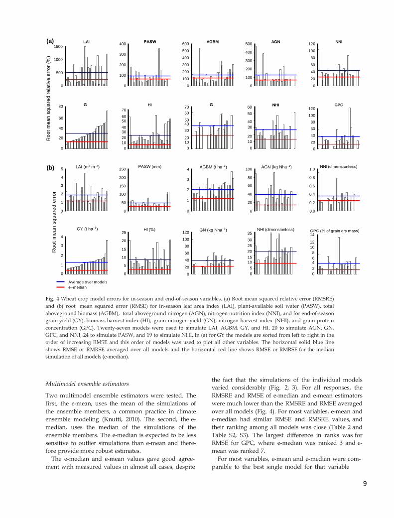
The RMSRE averaged over all models was 29%

(Fig. 4a and Table S2), and the RMSE average over all

models was 1.25 t DM ha-1 for GY (Fig. 4b and Table

2 and Table S3). The uncertainty in simulated GY was

large, with RMSRE ranging from 8% to 73% among the

27 models, but 80% of the models had an RMSRE for

GY comprised between 14% and 47% (Fig. 4a). For the

other end-of-season variables RMSRE ranged from 7%

to 60% for HI (averaging 24%), 22% to 61% for GN

(averaging 38%), 15% to 52% for NHI (averaging 26%),

and 8% to 122% for GPC (averaging 34%; Fig. 4a). For

the in-season variables with multiple measurements

per site, the RMSRE ranged from 48% to 1496% for LAI,

37% to 355% for PASW, 41% to 542% for AGBM, 49% to

472% for AGN, and 16% to 104% for NNI (Fig. 4a). The

large variability between models occurs because the

models have different equations for many functions (as

shown in Asseng et al. (2013) Table S2 in Supplemen-

tal) and different parameter values (Challinor et al.,

2014).

Of the three models with the smallest RMSE for GY,

only the second-ranked model had RMSE values

below the average of all models for all variables con-

sidered (Table 2). The other two models had an RMSE

substantially higher than the average for at least one

variable. The first- and second-ranked mod- els

simulated GY closely because of compensating errors.

They underestimated LAI around anthesis and final

AGBM which was compensated for by overesti-

mating HI. For instance, the first-ranked model simu-

lated that the canopy intercepted 83%, 74% and 51% of

the incident radiation around anthesis in AR, IN and

NL, respectively, while according to measured LAI

values the percentage of radiation interception was

close to 93% at the three sites (assuming an extinction

coefficient of 0.55, an average value reported for wheat

canopies (Sylvester-Bradley et al., 2012)). This model

compensated by having unrealisti- cally high HI

values that were 19% to 93% higher than measured

HI. Theoretical maximum HI has been estimated at

62–64% for wheat (Foulkes et al., 2011), while this

model had simulated values up to 69% (in NL). The

third-ranked model showed no significant

compensation of errors. This model overestimated LAI

around anthesis by 16% in AR and NL, but this

translated into only a small effect on intercepted radi-

ation, since the canopy intercepted more than 90% of

incident radiation based on observed LAI.

Relation between the error for grain yield and that for underlying variables

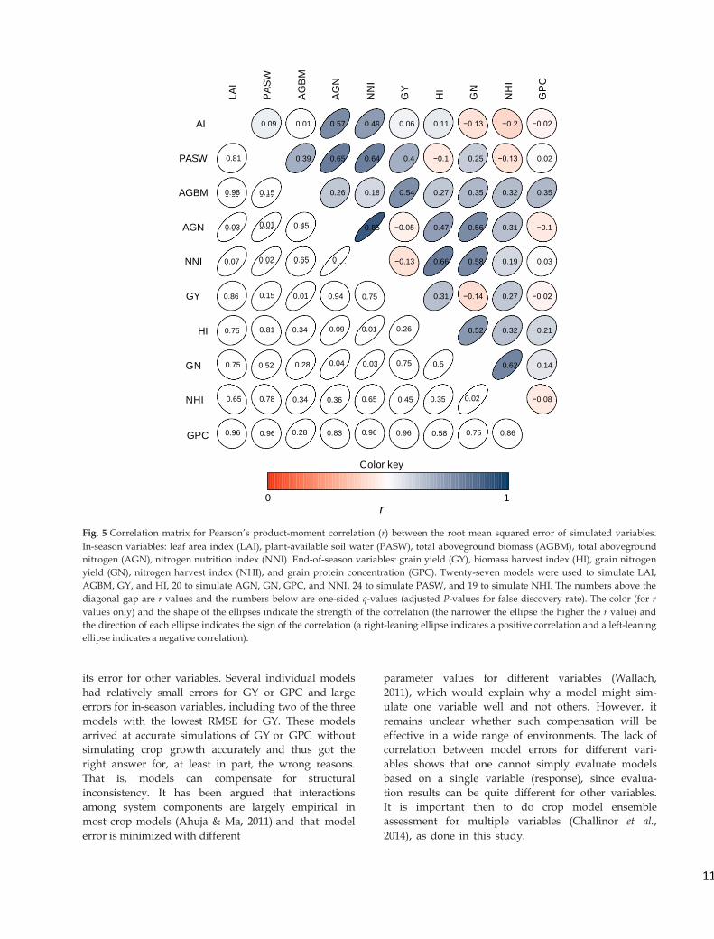
There was little relation between the errors for differ-

ent variables (Fig. 4a, b). There were some excep- tions,

however. Notably, RMSE for AGBM was highly

correlated with that for GY, and that for AGN was

correlated with GN (Fig. 5). Similarly, RMSE for

AGN was highly correlated with that for LAI, PASW,

and NNI. Finally, RMSE for NNI was correlated with

that for PASW, HI, and GN and to a lesser extent with

that for NNI. RMSE for GPC was not signifi- cantly

correlated with any other variable. Overall, the

correlations between RMSRE for different variables

were similar to that between RMSE for different vari-

ables (Fig. S1).

(a)

(b)

NL AR IN AU

GY

(t

ha1)

GP

C (

% o

f g

rain

dry

ma

ss)

9

LAI (m2 m2) AGBM (t ha1) AGN (kg Nha1)

(a)

1500

1000

500

0

400

300

200

100

0

600

500

400

300

200

100

0

500

400

300

200

100

0

120

100

80

60

40

20

0

80 70

60 60 50

40 40 30

20 20

10

0 0

70 60

60 50

50 40 40

30 30

20 20

10 10

0 0

120

100

80

60

40

20

0

(b) 5

4

3

2

1

250

200

150

100

50

4 100

3 80

60 2

40

1 20

1.0

0.8

0.6

0.4

0.2

0 0 0

0 0.0

GY (t ha1)

25 4

20

3 15

2 10

1 5

0 0

Average over models

e−median

120

100

80

60

40

20

0

35 GPC (% of grain dry mass) 14

30 12

25 10

20 8

15 6

10 4

5 2

0 0

Fig. 4 Wheat crop model errors for in-season and end-of-season variables. (a) Root mean squared relative error (RMSRE)

and (b) root mean squared error (RMSE) for in-season leaf area index (LAI), plant-available soil water (PASW), total

aboveground biomass (AGBM), total aboveground nitrogen (AGN), nitrogen nutrition index (NNI), and for end-of-season

grain yield (GY), biomass harvest index (HI), grain nitrogen yield (GN), nitrogen harvest index (NHI), and grain protein

concentration (GPC). Twenty-seven models were used to simulate LAI, AGBM, GY, and HI, 20 to simulate AGN, GN,

GPC, and NNI, 24 to simulate PASW, and 19 to simulate NHI. In (a) for GY the models are sorted from left to right in the

order of increasing RMSE and this order of models was used to plot all other variables. The horizontal solid blue line

shows RMSE or RMRSE averaged over all models and the horizontal red line shows RMSE or RMRSE for the median

simulation of all models (e-median).

Multimodel ensemble estimators

Two multimodel ensemble estimators were tested. The

first, the e-mean, uses the mean of the simulations of

the ensemble members, a common practice in climate

ensemble modeling (Knutti, 2010). The second, the e-

median, uses the median of the simulations of the

ensemble members. The e-median is expected to be less

sensitive to outlier simulations than e-mean and there-

fore provide more robust estimates.

The e-median and e-mean values gave good agree-

ment with measured values in almost all cases, despite

the fact that the simulations of the individual models

varied considerably (Fig. 2, 3). For all responses, the

RMSRE and RMSE of e-median and e-mean estimators

were much lower than the RMSRE and RMSE averaged

over all models (Fig. 4). For most variables, e-mean and

e-median had similar RMSE and RMSRE values, and

their ranking among all models was close (Table 2 and

Table S2, S3). The largest difference in ranks was for

RMSE for GPC, where e-median was ranked 3 and e-

mean was ranked 7.

For most variables, e-mean and e-median were com-

parable to the best single model for that variable

LAI AGBM AGN NNI

NHI GPC

GN (kg Nha1)

Ro

ot

me

an

sq

ua

red

re

lative

err

or

(%)

Ro

ot

me

an

sq

ua

red

err

or

10

(Fig. 4a, b). When e-median was ranked with the other

models based on RMSRE, it ranked fourth for GY and

third for GPC (Table S2); and first for GY and third for GPC

when ranked based on RMSE (Table S3). One way to

quantify the overall skill of e-mean and e-median is to

consider the sum of ranks over all the variables. The sum of

ranks based on RMSE for the 10 variables ana- lyzed in this

study was 37 for e-median and 45 for e-mean, while the

lowest sum of ranks for an individ- ual model (among the

17 models that simulated all variables) was 53 (Table S2). If

we only considered the four variables simulated by all 27

models (i.e. LAI, AGBM, GY, and HI), the sum of ranks for

e-median and e-mean was 15 and 17, respectively, while the

best sum of ranks for an individual model with these four

variables was 28.

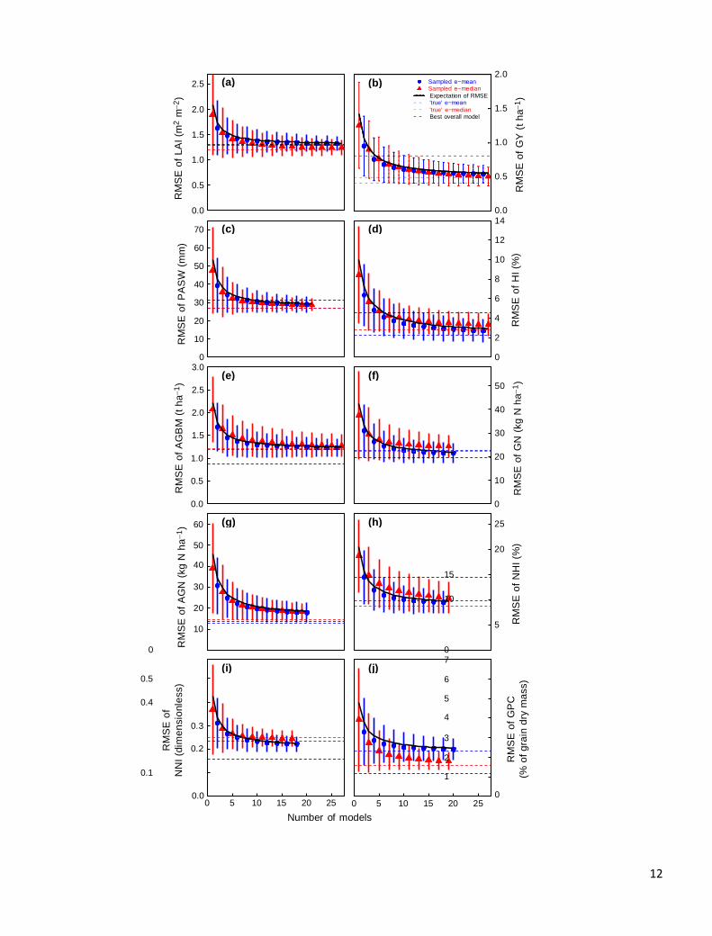
To analyze the relationship between the number of

models in an ensemble and the RMSE of both e-mean and

e-median, we used a bootstrap approach to create a large

number of ensembles for different multi-model ensemble

sizes M’. For each M’, the RMSE of both e-mean and e-

median in each bootstrap ensemble was calculated and

averaged over bootstrap samples (Fig. 6). The standard

deviation of RMSE for each M’ shows how RMSE varies

depending on the models that are included in the sample.

The bootstrap average for e-mean followed very closely the

theoretical expecta- tion of RMSE (Fig. 6). The average

RMSE of e-median also decreased with the number of

models, in a manner similar to, but not identical to, the

average e-mean RMSE. The differences were most

pronounced for GPC (Fig. 6j).

Discussion

Working with multimodel ensembles is well-estab- lished

in climate modeling, but only recently has the necessary

international coordination been developed to make this also

possible for crop models (Rosenzweig et al., 2013). Here,

we examined the performance of an ensemble of 27 wheat

models, created in the context of the AgMIP Wheat Pilot

study (Asseng et al., 2013). Mul- tiple crop responses,

including both end-of-season and in-season growth

variables were considered. Among these, GY and GPC are

the main determinants of wheat productivity and end-use

value. The other variables helped indicate whether models

are realistic and con- sistent in their description of the

processes leading to GY and GPC. This provides more

comprehensive infor- mation on crop system properties

beyond GY and is essential for the analysis of adaptation

and mitigation strategies to global changes (Challinor et al.,

2014).

In only a few cases there were significant correla- tions

between a model’s error for one variable and

Ta

ble

2

RM

SE

fo

r in

-sea

son

an

d e

nd

-of-

sea

son

va

ria

ble

s. E

nse

mb

le a

ver

ag

es

an

d e

-mea

n a

nd

e-m

edia

n v

alu

es a

re b

ase

d o

n 2

7 d

iffe

ren

t m

od

els

for

LA

I, A

GB

M,

GY

, a

nd

HI;

24

fo

r P

AS

W,

20

fo

r A

GN

, G

N,

GP

C,

an

d N

NI;

an

d 1

9 f

or

NH

I. V

alu

es f

or

the

thre

e b

est

mo

del

s fo

r G

Y (

ba

sed

on

RM

SE

) si

mu

lati

on

are

als

o g

iven

. D

ata

fo

r ea

ch i

nd

ivid

ua

l

mo

del

are

giv

en i

n T

ab

le S

4.

Th

e n

um

ber

s in

pa

ren

thes

is i

nd

ica

te t

he

ran

k o

f th

e m

od

els

(in

clu

din

g e

-mea

n a

nd

e-m

edia

n)

wh

ere

1 i

nd

ica

tes

the

mo

del

wit

h t

he

low

est

RM

SE

(i.e

. b

est

ran

k)

for

tha

t v

ari

ab

le.

Fo

r ea

ch v

ari

ab

le t

he

mo

del

wit

h t

he

low

est

RM

SE

is

in b

old

ty

pe.

RM

SE

fo

r in

-sea

son

va

ria

ble

s R

MS

E f

or

end

-of-

sea

son

va

ria

ble

s

LA

I

(m-

2 m-

2)

1.9

0

2.3

1 (

23

)

1.2

4 (

7)

1.7

5 (

16

)

1.2

0 (

6)

1.2

9 (

8)

PA

SW

(mm

)

AG

BM

(t D

M h

a-

1)

2.0

7

2.2

6 (

17

)

1.7

1 (

13

)

1.0

1 (

3)

1.2

0 (

6)

1.1

9 (

5)

AG

N

(kg

N h

a-

1)

39

89

(2

1)

24

(8

)

22

(7

)

15

(3

)

13

(1

)

NN

I

(-)

GY

(t D

M h

a-

1)

1.2

5

0.4

2 (

2)

0.5

6 (

4)

0.6

3 (

5)

0.4

1 (

1)

0.4

9 (

3)

HI

(%)

GN

(kg

N h

a-

1)

38

10

0 (

22

)

27

(9

)

29

(1

0)

22

(5

)

23

(6

)

NH

I

(%)

GP

C

(% o

f g

rain

DM

) E

stim

ato

r

Av

era

ge

ov

er a

ll m

od

els

Mo

del

ra

nk

ed 1

fo

r G

Y

Mo

del

ra

nk

ed 2

fo

r G

Y

Mo

del

ra

nk

ed 3

fo

r G

Y

e-m

edia

n

e-m

ean

47

60

(2

1)

36

(9

)

63

(2

2)

27

(3

)

27

(5

)

0.3

5

0.9

2 (

22

)

0.2

6 (

8)

0.2

1 (

4)

0.2

5 (

7)

0.2

4 (

6)

8.5

20

.0 (

28

)

7.2

(1

6)

3.8

(5

)

2.8

(2

)

2.2

(1

)

18

.7

23

.6 (

18

)

9.1

(2

)

11

.7 (

5)

8.8

(1

)

9.8

(3

)

3.9

3

6.9

1 (

21

)

2.7

5 (

9)

2.1

3 (

6)

1.5

7 (

3)

2.3

2 (

7)

11

AI

PASW

AGBM

AGN

NNI

GY

HI

GN

NHI

GPC

Color key

0 1

r

Fig. 5 Correlation matrix for Pearson’s product-moment correlation (r) between the root mean squared error of simulated variables.

In-season variables: leaf area index (LAI), plant-available soil water (PASW), total aboveground biomass (AGBM), total aboveground

nitrogen (AGN), nitrogen nutrition index (NNI). End-of-season variables: grain yield (GY), biomass harvest index (HI), grain nitrogen

yield (GN), nitrogen harvest index (NHI), and grain protein concentration (GPC). Twenty-seven models were used to simulate LAI,

AGBM, GY, and HI, 20 to simulate AGN, GN, GPC, and NNI, 24 to simulate PASW, and 19 to simulate NHI. The numbers above the

diagonal gap are r values and the numbers below are one-sided q-values (adjusted P-values for false discovery rate). The color (for r

values only) and the shape of the ellipses indicate the strength of the correlation (the narrower the ellipse the higher the r value) and

the direction of each ellipse indicates the sign of the correlation (a right-leaning ellipse indicates a positive correlation and a left-leaning

ellipse indicates a negative correlation).

its error for other variables. Several individual models

had relatively small errors for GY or GPC and large

errors for in-season variables, including two of the three

models with the lowest RMSE for GY. These models

arrived at accurate simulations of GY or GPC without

simulating crop growth accurately and thus got the

right answer for, at least in part, the wrong reasons.

That is, models can compensate for structural

inconsistency. It has been argued that interactions

among system components are largely empirical in

most crop models (Ahuja & Ma, 2011) and that model

error is minimized with different

parameter values for different variables (Wallach,

2011), which would explain why a model might sim-

ulate one variable well and not others. However, it

remains unclear whether such compensation will be

effective in a wide range of environments. The lack of

correlation between model errors for different vari-

ables shows that one cannot simply evaluate models

based on a single variable (response), since evalua-

tion results can be quite different for other variables.

It is important then to do crop model ensemble

assessment for multiple variables (Challinor et al.,

2014), as done in this study.

0.09 0.01 0.57 0.49 0.06 0.11 −0.13 −0.2 −0.02

0.39 0.65 0.64 0.4 −0.1 0.25 −0.13 0.02

0.26 0.18 0.54 0.27 0.35 0.32 0.35

0.85 −0.05 0.47 0.56 0.31 −0.1

−0.13 0.66 0.58 0.19 0.03

0.31 −0.14 0.27 −0.02

0.52 0.32 0.21

0.62 0.14

−0.08

LA

I

PA

SW

AG

BM

AG

N

NN

I

GY

HI

GN

NH

I

GP

C

0.81

0.98 0.81

0.15 0.81

0.03 0.81

0.01 0.81

0.45 0.81

0.07 0.81

0.02 0.81

0.65 0.81

0 0.81

0.86 0.15 0.01 0.94 0.75

0.75 0.81 0.34 0.09 0.01 0.26

0.75 0.52 0.28 0.04 0.03 0.75 0.5

0.65 0.78 0.34 0.36 0.65 0.45 0.35 0.02

0.96 0.96 0.28 0.83 0.96 0.96 0.58 0.75 0.86

12

(e)

(g)

(i)

(f)

(h)

(j)

2.5

2.0

2.0 1.5

1.5

1.0

0.5

1.0

0.5

0.0

70

60

50

40

30

20

10

0 3.0

2.5

2.0

1.5

0.0 14

12

10

8

6

4

2

0

50

40

30

1.0 20

0.5 10

0.0 0

60 25

50 20

40 15

30

10 20

10 5

0 0 7

0.5 6

0.4 5

4 0.3

3

0.2 2

0.1 1

0.0 0 5 10 15 20 25

0

0 5 10 15 20 25

Number of models

(a)

(c)

(b) Sampled e−mean Sampled e−median

Expectation of RMSE'true' e−mean

'true' e−medianBest overall model

(d)

RM

SE

of

NN

I (d

ime

nsio

nle

ss)

RM

SE

of

AG

BM

(t

ha1)

RM

SE

of

LA

I (m

2 m

2)

RM

SE

of

AG

N (

kg N

ha1)

RM

SE

of

PA

SW

(m

m)

RM

SE

of

GP

C

(% o

f g

rain

dry

ma

ss)

RM

SE

of

NH

I (%

) R

MS

E o

f G

N (

kg N

ha

1)

RM

SE

of

HI

(%)

RM

SE

of

GY

(t

ha1)

13

Fig. 6 How the number of models in an ensemble affects error estimates. Average root mean squared error (RMSE) (± 1 s.d.) of e-mean

and e-median for in-season (a) leaf area index (LAI), (c) plant-available soil water (PASW), (e) total aboveground biomass (AGBM), (g)

total aboveground nitrogen (AGN), and (i) nitrogen nutrition index (NNI) and for end-of-season (b) grain yield (GY), (d) biomass har-

vest index (HI), (f) grain nitrogen yield (GN), (h) nitrogen harvest index (NHI), and (j) grain protein concentration (GPC) vs. number of

models in the ensemble. Values are calculated based on 12,800 bootstrap samples. The solid line is the analytical result for RMSE as a

function of sample size (equation (8)). The blue dashed line shows the RMSE for e-mean and the red dashed line the RMSE for e-med-

ian of the multimodel ensemble. The black dashed line is the RMSE for the individual model with lowest sum of ranks for RMSE. For

visual clarity the RMSE for e-mean is plotted for even numbers of models, and the RMSE for e-median for odd numbers of models.

Compensation of errors may be related to the way

models are calibrated. If they are calibrated using only

observed variable, e.g. GY, this may give parameter

values that lead to unrealistic values of intermediate

variables. The calibration insures that any errors in the

intermediate variables compensate however, so that GY

values are reasonably well-simulated. If final results are

not used in calibration, for example if GPC is not used

for calibration, then there may be compensation or

compounding of the errors in the intermediate vari-

ables that lead to GPC.

There does not seem to be any simple relationship

between model structure or the approach used to simu-

late individual processes and model error. Asseng et al.

(2013) analyzed the response of the 27 crop models

used in this study to a short heat shock around anthesis

(seven consecutive days with a maximum daily temper-

ature of 35 °C) and found that accounting for heat

stress impact does not necessarily result in correctly

simulating that effect. Similarly, we found that even

closely related models did not necessarily cluster

together and no single process could account for model

error (data not shown). Therefore, it seems that model

performances are not simply related to how a single

process is modeled, but rather to the overall structure/

parameterization of the model.

The behavior of the median and mean of the ensem-

ble simulations was similar. Both estimators had much

smaller errors and better skills than that averaged over

models, for all variables. In comparing the sum of ranks

of error for all variables, which provides an aggregated

performance measure, the e-median was better than e-

mean, but most importantly both were superior to even

the best performing model in the ensemble. Differ- ent

measures of performance might give slightly differ- ent

results, but would not change the fact that e-median

and e-mean compare well with even the best models.

E-mean and e-median had small errors in simulating

not only end-of-season variables but also in-season

variables. This suggests that multimodel ensembles

could be useful not only for simulating GY and GPC,

but also for relating those results to in-season growth

processes. This is important if crop model ensembles are

to be useful in exploring the consequences of global

change and the benefits of adaptation or mitigation

strategies.

A fundamental question is the origin of the advan-

tage of ensemble predictors over individual models.

Two possible explanations relate to compensation

among errors in processes descriptions and to more

coverage of the possible crop and soil phase spaces. The

first possible explanation is that certain models had

large errors with compensations to achieve a reasonable

yield simulation. In those cases, e-median can supply a

better estimate when multiple responses are consid-

ered, since it gives reasonable results for all variables.

In other cases, it is simply the fact that the errors in the

different models tend to compensate each other well,

that makes e-median the best estimator over multiple

responses. The compensation of errors among models

comes, at least in part, from the fact that models do not

produce random outputs but are driven by environ-

mental and management inputs and bio-physical pro-

cesses and therefore they tend to converge to the

measured crop response. It is an open question, how-

ever, as to whether the superiority of crop model

ensemble estimators compared to individual models

extends to conditions not tested in this study. Will this

still be the case if the models are used to predict the

impact of climate change? Or, will multimodel ensem-

bles also be better capable than individual models to

simulate the impact of interannual variability in

weather at one site?

The second possible explanation relates to phase-

space coverage. For climate models, the main reason for

the superiority of multimodel ensemble estimators is

that better coverage of the whole possible climate phase

space leads to greater consistency (Hagedorn et al.,

2005). An analogous advantage holds as well for crop

model ensembles, they have more associated

knowledge and represent more processes than any

individual model. Each of the individual models has

been developed and calibrated based on a limited data-

set. The ensemble simulators are in a sense averaging

over these datasets, which gives them the advantage of

a much broader database than any individual model

and thus reduces the need for site- and varietal-specific

model calibration.

14

The use of ensemble estimators to answer new ques-

tions in the future poses specific questions regarding

the best procedure for creating an ensemble. Several of

these questions have been debated in the climate sci-

ence community (Knutti, 2010), but not always in a way

that is directly applicable to crop models. One question

is how performance varies with the number of models

in the ensemble. Here we found that the change in

ensemble error (MSEM’) with the number of model in

an ensemble (M’) follows the expectation of MSE. Thus when planning ensemble studies, one can estimate the potential reduction in MSEM’ and therefore, do a costs

vs. benefits analysis for increasing M’. In the ensemble

studied here, for all the variables, MSE for an ensemble

of 10 models was close to the asymptotic limit for very large M’.

Other questions include how to choose the models in

the ensemble, and whether one should weight the mod-

els in the ensemble differently, based on past perfor-

mance and convergence for new situations (Tebaldi &

Knutti, 2007). In this respect, the crop modeling com-

munity might employ some of the ensemble weighting

methods developed by the climate modeling commu-

nity (Christensen et al., 2010). There are also questions

about the possible multiple uses of models. Would it be

advantageous to have multiple simulations, based on a

diversity of initial conditions (including ‘spin-up’ peri-

ods for models that depend on simulation of changes in

soil organic matter) or multiple parameter sets from

each model? In any case, the first step is to document

the accuracy of multimodel ensemble estimators in spe-

cific situations, as done here.

In summary, by reducing simulation error and

improving the consistency of simulation results for

multiple variables, crop model ensembles could sub-

stantially increase the range of questions that could be

addressed. A lack of correlation between end-of-season

and in-season errors in the individual models indicates

that further work is needed to improve the representa-

tion of the dynamics of growth and development pro-

cesses leading to GY in crop models. This is crucial for

their application under changed climatic or manage-

ment conditions.

Most of the physical and physiological processes that

are simulated in wheat models are the same as for other

crops. In fact, several of the models in this study have a

generic structure so that they can be applied to various

crops, and for some of them the differences between

crops are simply in the parameter values. It is thus rea-

sonable to expect that the results obtained here for

wheat are broadly applicable to other crop species. It

would be worthwhile to study whether these results

also apply more generally to biological and ecological

system models.

Acknowledgements

P.M. is grateful to the INRA metaprogram ‘Adaptation of Agri- culture and Forests to Climate Change’ and Environment and Agronomy Division for supporting several stays at the Univer-

sity of Florida during this work.

References

Ahuja LR, Ma L (2011) A synthesis of current parameterization approaches and needs

for further improvements. In: Methods of Introducing System Models into Agricultural

Research (eds Ahuja LR, Ma L), pp. 427–440. American Society of Agronomy, Crop

Science Society of America, Soil Science Society of America, Madison, WI.

Angulo C, Ro€tter R, Lock R, Enders A, Fronzek S, Ewert F (2013) Implication of crop

model calibration strategies for assessing regional impacts of climate change in

Europe. Agricultural and Forest Meteorology, 170, 32–46.

Asseng S, Keating BA, Fillery IRP et al. (1998) Performance of the APSIM-wheat

model in Western Australia. Field Crops Research, 57, 163–179.

Asseng S, Ewert F, Rosenzweig C et al. (2013) Uncertainty in simulating wheat yields

under climate change. Nature Climate Change, 3, 827–832.

Bassu S, Brisson N, Durand J-L et al. (2014) How do various maize crop models vary

in their responses to climate change factors? Global Change Biology, 20, 2301–2320.

Bellocchi G, Rivington M, Donatelli M, Matthews K (2010) Validation of biophysical

models: issues and methodologies. A review. Agronomy for Sustainable Develop-

ment, 30, 109–130.

Bertin N, Martre P, Genard M, Quilot B, Salon C (2010) Under what circumstances

can process-based simulation models link genotype to phenotype for complex

traits? Case-study of fruit and grain quality traits. Journal of Experimental Botany,

61, 955–967.

Bloom DE (2011) 7 Billion and Counting. Science, 333, 562–569.

Bosilovich MG, Robertson FR, Chen JY (2011) Global energy and water budgets in

MERRA. Journal of Climate, 24, 5721–5739.

Challinor AJ, Wheeler T, Hemming D, Upadhyaya HD (2009) Ensemble yield simula-

tions: crop and climate uncertainties, sensitivity to temperature and genotypic

adaptation to climate change. Climate Research, 38, 117–127.

Challinor A, Martre P, Asseng S, Thornton P, Ewert F (2014) Making the most of cli-

mate impacts ensembles. Nature Climate Change, 4, 77–80.

Christensen JH, Kjellstro€m E, Giorgi F, Lenderink G, Rummukainen M (2010) Weight

assignment in regional climate models. Climate Research, 44, 179–194. Dalmasso C, Bro€et P, Moreau T (2005) A simple procedure for estimating the

false discovery rate. Bioinformatics, 21, 660–668.

Easterling WE, Aggarwal PK, Batima P et al. (2007) Food, fibre and forest products.

In: Climate Change 2007: Impacts, Adaptation and Vulnerability. Contribution of Work-

ing Group II to the Fourth Assessment Report of the intergovernmental Panel on Climate

Change (eds Parry ML, Canziani OF, Palutikof JP, Van De Linden P, Hanson CE),

pp. 273–313. Cambridge University Press, Cambridge, UK.

FAOSTAT (2014) Food and Agricultural organization of the United Nations (FAO).

FAO Statistical Databases. Available at: faostat3.fao.org (accessed 28 October

2014).

Foulkes MJ, Slafer GA, Davies WJ et al. (2011) Raising yield potential of wheat. III.

Optimizing partitioning to grain while maintaining lodging resistance. Journal of

Experimental Botany, 62, 469–486.

Godfray HCJ, Beddington JR, Crute IR et al. (2010) Food security: the challenge of

feeding 9 billion people. Science, 327, 812–818.

Gonzalez-Dugo V, Durand J-L, Gastal F (2010) Water deficit and nitrogen nutrition of

crops. A review. Agronomy for Sustainable Development, 30, 529–544.

Grenouillet G, Buisson L, Casajus N, Lek S (2011) Ensemble modelling of species dis-

tribution: the effects of geographical and environmental ranges. Ecography, 34, 9–17.

Groot JJR, Verberne ELJ (1991) Response of wheat to nitrogen fertilization, a data set

to validate simulation models for nitrogen dynamics in crop and soil. In: Nitrogen

Turnover in the Soil-Crop System. Modelling of Biological Transformations, Transport of

Nitrogen and Nitrogen Use Efficiency. Proceedings of a Workshop (eds Groot JJR, De

Willigen P, Verberne ELJ), pp. 349–383. Institute for Soil Fertility Research, Haren,

The Netherlands.

Hagedorn T, Doblas-Reyes FJ, Palmer TN (2005) The rationale behind the success of

multi-model ensembles in seasonal forecasting – I. Basic concept. Tellus, 57A, 219–

233.

Justes E, Mary B, Meynard JM, Machet JM, Thelier-Huche L (1994) Determination of

a critical nitrogen dilution curve for winter wheat crops. Annals of Botany, 74, 397–

407.

15

Knutti R (2010) The end of model democracy? An editorial comment. Climatic Change,

102, 395–404.

Ko J, Ahuja L, Kimball B et al. (2010) Simulation of free air CO2 enriched wheat

growth and interactions with water, nitrogen, and temperature. Agricultural and

Forest Meteorology, 150, 1331–1346.

Lemaire G, Gastal F (1997) N uptake and distribution in plant canopies. In: Diagnosis

of the Nitrogen Status in Crops (ed. Lemaire G), pp. 3–43. Springer Verlag, Berlin,

Germany.

Lemaire G, Jeuffroy M-H, Gastal F (2008) Diagnosis tool for plant and crop N status

in vegetative stage: theory and practices for crop N management. European Journal

of Agronomy, 28, 614–624.

Lobell DB, Schlenker W, Costa-Roberts J (2011) Climate trends and global crop pro-

duction since 1980. Science, 333, 616–620.

Naveen N (1986) Evaluation of soil water status, plant growth and canopy environ-

ment in relation to variable water supply to wheat. Unpublished PhD, IARI, New

Delhi.

Palosuo T, Kersebaum KC, Angulo C et al. (2011) Simulation of winter wheat yield

and its variability in different climates of Europe: a comparison of eight crop

growth models. European Journal of Agronomy, 35, 103–114.

Porter JR, Semenov MA (2005) Crop responses to climatic variation. Philosophical

Transactions of the Royal Society of London B Biological Sciences, 360, 2021–2035.

R Core Team (2013) R: A Language and Environment for Statistical Computing. R Foun-

dation for Statistical Computing, Vienna, Austria.

R€ais€anen J, Palmer TN (2001) A probability and decision-model analysis of a

multimodel ensemble of climate change simulations. Journal of Climate, 14,

3212–3226.

Rosenzweig C, Elliott J, Deryng D et al. (2014) Assessing agricultural risks of climate

change in the 21st century in a global gridded crop model intercomparison. Pro-

ceedings of the National Academy of Sciences, 111, 3268–3273.

Rosenzweig C, Jones JW, Hatfield JL et al. (2013) The Agricultural Model Intercom-

parison and Improvement Project (AgMIP): protocols and pilot studies. Agricul-

tural and Forest Meteorology, 170, 166–182.

Ro€tter RP, Carter TR, Olesen JE, Porter JR (2011) Crop-climate models need an over-

haul. Nature Climate Change, 1, 175–177.

Ro€tter RP, Palosuo T, Kersebaum KC et al. (2012) Simulation of spring barley yield in

different climatic zones of Northern and Central Europe: a comparison of nine

crop models. Field Crops Research, 133, 23–36.

Stackhouse P (2006) Prediction of worldwide energy resources. Available at: http://

power.larc.nasa.gov (accessed 28 October 2014).

Sylvester-Bradley R, Riffkin P, O’leary G (2012) Designing resource-efficient ideo-

types for new cropping conditions: wheat (Triticum aestivum L.) in the High Rain-

fall Zone of southern Australia. Field Crops Research, 125, 69–82.

Tebaldi C, Knutti R (2007) The use of the multi-model ensemble in probabilistic cli-

mate projections. Philosophical Transactions of the Royal Society A: Mathematical,

Physical and Engineering Sciences, 365, 2053–2075.

Travasso MI, Magrin GO, Rodr'ıguez R, Grondona MO (2005) Comparing

CERES-wheat and SUCROS2 in the Argentinean Cereal Region. In: MODSIM

2005 International Congress on Modelling and Simulation (eds Zerger A, Argent

RM), pp. 366–369. Modelling and Simulation Society of Australia and New

Zealand. Available at: http://www.mssanz.org.au/MODSIM95/Vol%201/Tra-

vasso.pdf. (accessed 28 October 2014)

Trewavas A (2006) A brief history of systems biology: “every object that biology stud-

ies is a system of systems”. Francois Jacob (1974). Plant Cell, 18, 2420–2430.

Tubiello FN, Soussana J-F, Howden SM (2007) Crop and pasture response to climate

change. Proceedings of the National Academy of Sciences, 104, 19686–19690.

Wallach D (2011) Crop Model Calibration: a Statistical Perspective. Agronomy Journal,

103, 1144–1151.

Wallach D, Makowski D, Jones JW, Brun F (2013) Working with Dynamic Crop Models.

Methods Tools and Examples for Agriculture and Environment. Academic Press, London.

White JW, Hoogenboom G, Kimball BA, Wall GW (2011) Methodologies for simulat-

ing impacts of climate change on crop production. Field Crops Research, 124,

357–368.

Zadoks JC, Chang TT, Konzak CF (1974) A decimal code for the growth stages of

cereals. Weed Research, 14, 415–421.