Origins & Evolution of the Universean introduction to cosmology — Fall 2018

Rychard Bouwens

Origins'&'Evolu.on'of'the'Universe'an'introduc.on'to'cosmology'–'Fall'2016'

Henk'Hoekstra'&'Andrej'Dvornik'hDp://www.strw.leidenuniv.nl/~hoekstra/TEACHING/OEU/OEU.html'

This'course'in'the'cosmology'track'

Related'courses'

Observa.onal'cosmology' 3'EC'

Theore.cal'cosmology' 3'EC'

Core'courses'for'the'MSc'cosmology'track''

Origin'and'Evolu.on'of'the'Universe' 6'EC'

Par.cle'Physics'and'Early'Universe' 6'EC'

Large'Scale'Structure'and'Galaxy'Forma.on' 6'EC'

Theory'of'General'Rela.vity' 6'EC'

Although'General'Rela.vity'is'cri.cal'to'understand'our'Universe,'we'can'do'without'

for'the'moment.'We'will'assume'a'basic'BSc'level'knowledge'of'astronomy.'

Origins'and'Evolu.on'of' the'Universe' is' the' introduc.on'to'physical'cosmology'at'

Leiden'Universe.' The' course' can'be' taken'as' a' standZalone' course'and' requires' a'

minimum'of'preZrequisites.'

Lectures

Rychard BouwensOort 459

bouwens@strw.leidenuniv.nl

Course Website:http://www.strw.leidenuniv.nl/~bouwens/oeu/

Lecture Hours:Huygens 414

Monday 1:30-3:15

Layout of the Course

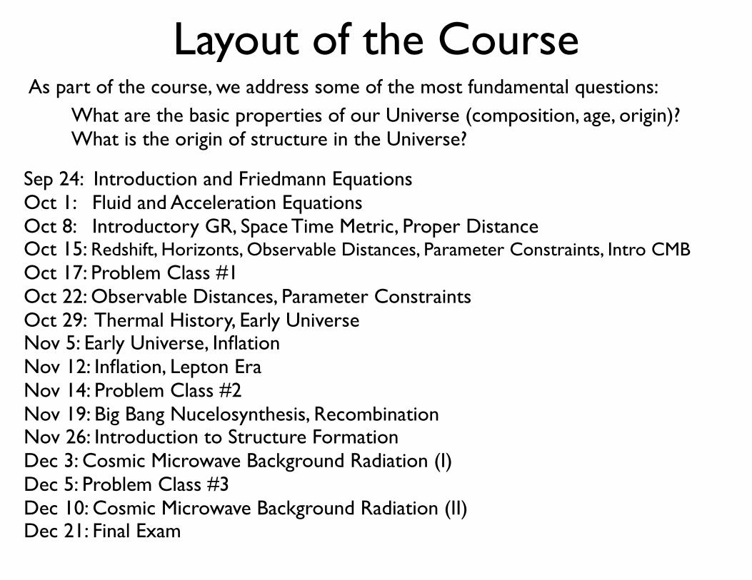
Sep 24: Introduction and Friedmann EquationsOct 1: Fluid and Acceleration EquationsOct 8: Introductory GR, Space Time Metric, Proper DistanceOct 15: Redshift, Horizonts, Observable Distances, Parameter Constraints, Intro CMBOct 17: Problem Class #1Oct 22: Observable Distances, Parameter ConstraintsOct 29: Thermal History, Early UniverseNov 5: Early Universe, InflationNov 12: Inflation, Lepton EraNov 14: Problem Class #2Nov 19: Big Bang Nucelosynthesis, RecombinationNov 26: Introduction to Structure FormationDec 3: Cosmic Microwave Background Radiation (I)Dec 5: Problem Class #3Dec 10: Cosmic Microwave Background Radiation (II)Dec 21: Final Exam

As part of the course, we address some of the most fundamental questions:What are the basic properties of our Universe (composition, age, origin)?What is the origin of structure in the Universe?

ExaminationA written exam is scheduled for December 21, 2018. The material covered in this class delimits what will be tested in the exam.

Do not forget to register for the exam in uSIS!

Problem ClassesTo aid in the preparation for the exam, there are three scheduled problem classes with the homework. This accounts for 20% of the grade, if it is higher than the result for the written exam.

The homework needs to be handed in before the start of the problem class.

Oct 17: Problem Class #1Oct 22: Observable Distances, Parameter ConstraintsOct 29: Thermal History, Early UniverseNov 5: Early Universe, InflationNov 12: Inflation, Leption EraNov 14: Problem Class #2Nov 19: Big Bang Nucelosynthesis, RecombinationNov 26: Introduction to Structure FormationDec 3: Cosmic Microwave Background Radiation (I)Dec 5: Problem Class #3Dec 10: Cosmic Microwave Background Radiation (II)Dec 21: Final Exam

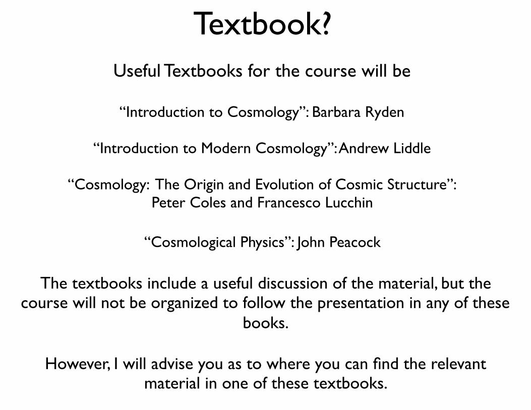
Textbook?Useful Textbooks for the course will be

“Introduction to Cosmology”: Barbara Ryden

“Introduction to Modern Cosmology”: Andrew Liddle

“Cosmology: The Origin and Evolution of Cosmic Structure”:Peter Coles and Francesco Lucchin

“Cosmological Physics”: John Peacock

The textbooks include a useful discussion of the material, but the course will not be organized to follow the presentation in any of these

books.

However, I will advise you as to where you can find the relevant material in one of these textbooks.

Who am I?

My name is Rychard Bouwens(studied in the United States: Berkeley & Santa Cruz)

I study the most distant galaxies in the universe

A good understanding of galaxies is very important for my research

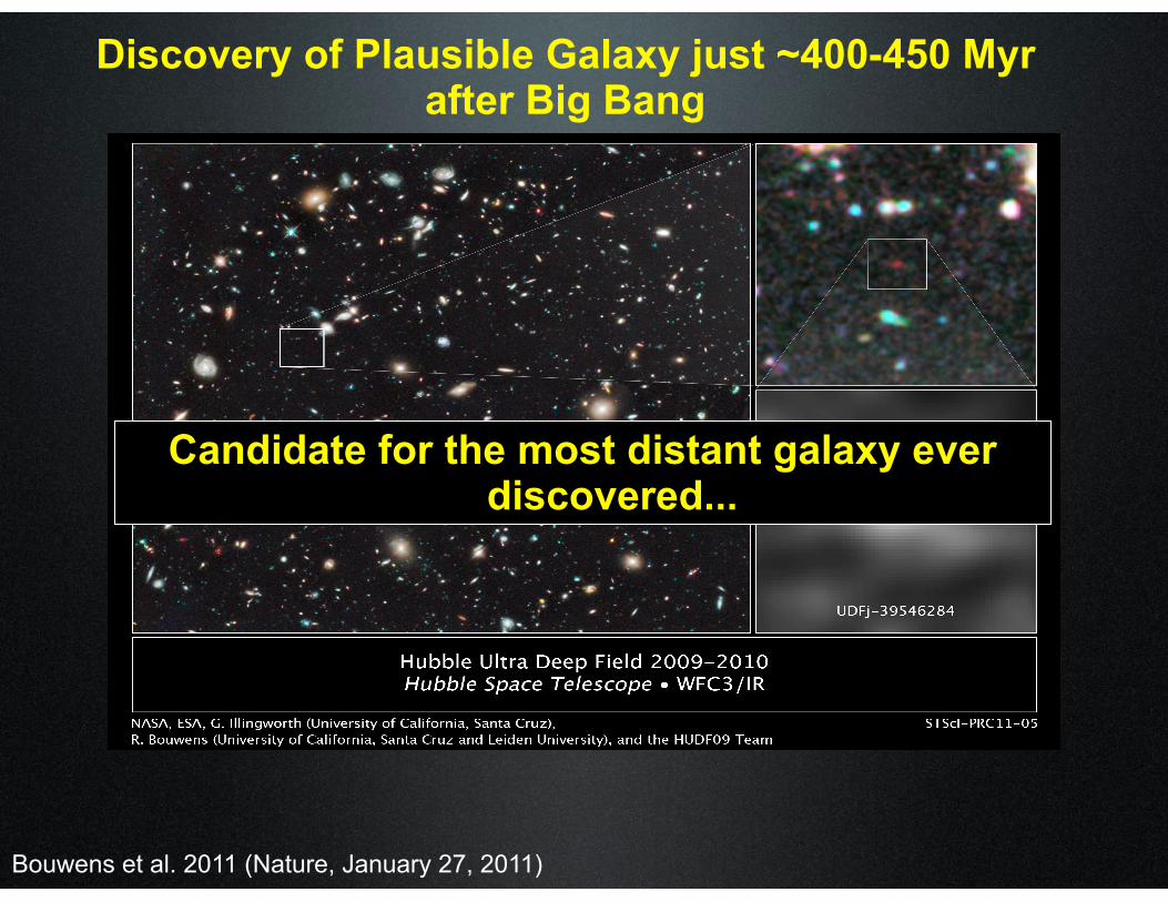
Bouwens et al. 2011 (Nature, January 27, 2011)

Discovery of Plausible Galaxy just ~400-450 Myr after Big Bang

Candidate for the most distant galaxy ever discovered...

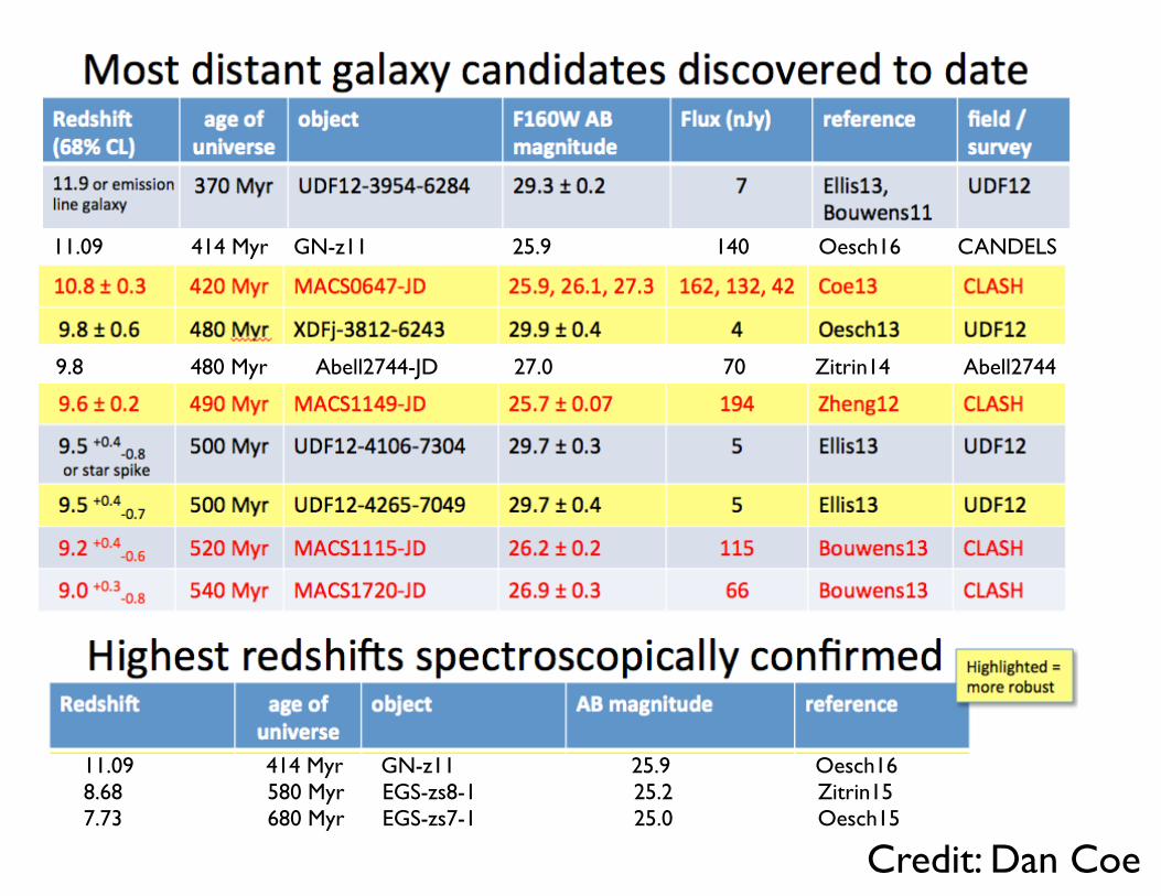
Credit: Dan Coe

9.8 480 Myr Abell2744-JD 27.0 70 Zitrin14 Abell2744

11.09 414 Myr GN-z11 25.9 Oesch168.68 580 Myr EGS-zs8-1 25.2 Zitrin157.73 680 Myr EGS-zs7-1 25.0 Oesch15

11.09 414 Myr GN-z11 25.9 140 Oesch16 CANDELS

Teaching Assistant

Anna de GraaffOort 532

graaff@strw.leidenuniv.nl

Anna should also be available by appointment to answer your questions.

Who are you?

Why don’t we go around the class and introduce ourselves briefly?

NameProgram -- Physics or Astronomy?

Master’s Student?First or Second Year?

Why interested in course?

What’s your background?

How many of you have taken Huub’s or Marijn’s course “Galaxies and Cosmology” when you were a

bachelor student?

How many of you are from the physics program?

Please ask questions

This is *your* course. It is your opportunity to learn.

By asking questions, you allow me to clarify issues

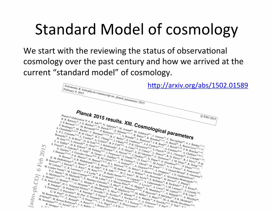
Standard'Model'of'cosmology'We'start'with'the'reviewing'the'status'of'observa.onal'cosmology'over'the'past'century'and'how'we'arrived'at'the'current'“standard'model”'of'cosmology.'

Astronomy & Astrophysics manuscript no. planck˙parameters˙2015

c� ESO 2015

February 9, 2015

Planck 2015 results. XIII. Cosmological parameters

Planck Collaboration: P. A. R. Ade100, N. Aghanim70, M. Arnaud84, M. Ashdown80,7, J. Aumont70, C. Baccigalupi99, A. J. Banday111,11,

R. B. Barreiro76, J. G. Bartlett1,78, N. Bartolo36,77, E. Battaner114,115, R. Battye79, K. Benabed71,110, A. Benoıt68, A. Benoit-Levy27,71,110,

J.-P. Bernard111,11, M. Bersanelli39,58, P. Bielewicz111,11,99, A. Bonaldi79, L. Bonavera76, J. R. Bond10, J. Borrill16,104, F. R. Bouchet71,102,

F. Boulanger70, M. Bucher1, C. Burigana57,37,59, R. C. Butler57, E. Calabrese107, J.-F. Cardoso85,1,71, A. Catalano86,83, A. Challinor73,80,14,

A. Chamballu84,18,70, R.-R. Chary67, H. C. Chiang31,8, J. Chluba26,80, P. R. Christensen94,43, S. Church106, D. L. Clements66, S. Colombi71,110,

L. P. L. Colombo25,78, C. Combet86, A. Coulais83, B. P. Crill78,95, A. Curto7,76, F. Cuttaia57, L. Danese99, R. D. Davies79, R. J. Davis79, P. de

Bernardis38, A. de Rosa57, G. de Zotti54,99, J. Delabrouille1, F.-X. Desert63, E. Di Valentino38, C. Dickinson79, J. M. Diego76, K. Dolag113,91,

H. Dole70,69, S. Donzelli58, O. Dore78,13, M. Douspis70, A. Ducout71,66, J. Dunkley107, X. Dupac46, G. Efstathiou80,73 ⇤, F. Elsner27,71,110,

T. A. Enßlin91, H. K. Eriksen74, M. Farhang10,97, J. Fergusson14, F. Finelli57,59, O. Forni111,11, M. Frailis56, A. A. Fraisse31, E. Franceschi57,

A. Frejsel94, S. Galeotta56, S. Galli71, K. Ganga1, C. Gauthier1,90, M. Gerbino38, T. Ghosh70, M. Giard111,11, Y. Giraud-Heraud1, E. Giusarma38,

E. Gjerløw74, J. Gonzalez-Nuevo76,99, K. M. Gorski78,117, S. Gratton80,73, A. Gregorio40,56,62, A. Gruppuso57, J. E. Gudmundsson31,

J. Hamann109,108, F. K. Hansen74, D. Hanson92,78,10, D. L. Harrison73,80, G. Helou13, S. Henrot-Versille81, C. Hernandez-Monteagudo15,91,

D. Herranz76, S. R. Hildebrandt78,13, E. Hivon71,110, M. Hobson7, W. A. Holmes78, A. Hornstrup19, W. Hovest91, Z. Huang10,

K. M. Hu↵enberger29, G. Hurier70, A. H. Ja↵e66, T. R. Ja↵e111,11, W. C. Jones31, M. Juvela30, E. Keihanen30, R. Keskitalo16, T. S. Kisner88,

R. Kneissl45,9, J. Knoche91, L. Knox33, M. Kunz20,70,3, H. Kurki-Suonio30,52, G. Lagache5,70, A. Lahteenmaki2,52, J.-M. Lamarre83, A. Lasenby7,80,

M. Lattanzi37, C. R. Lawrence78, J. P. Leahy79, R. Leonardi46, J. Lesgourgues109,98,82, F. Levrier83, A. Lewis28, M. Liguori36,77, P. B. Lilje74,

M. Linden-Vørnle19, M. Lopez-Caniego46,76, P. M. Lubin34, J. F. Macıas-Perez86, G. Maggio56, N. Mandolesi57,37, A. Mangilli70,81, A. Marchini60,

P. G. Martin10, M. Martinelli116, E. Martınez-Gonzalez76, S. Masi38, S. Matarrese36,77,49, P. Mazzotta41, P. McGehee67, P. R. Meinhold34,

A. Melchiorri38,60, J.-B. Melin18, L. Mendes46, A. Mennella39,58, M. Migliaccio73,80, M. Millea33, S. Mitra65,78, M.-A. Miville-Deschenes70,10,

A. Moneti71, L. Montier111,11, G. Morgante57, D. Mortlock66, A. Moss101, D. Munshi100, J. A. Murphy93, P. Naselsky94,43, F. Nati31, P. Natoli37,4,57,

C. B. Netterfield22, H. U. Nørgaard-Nielsen19, F. Noviello79, D. Novikov89, I. Novikov94,89, C. A. Oxborrow19, F. Paci99, L. Pagano38,60, F. Pajot70,

R. Paladini67, D. Paoletti57,59, B. Partridge51, F. Pasian56, G. Patanchon1, T. J. Pearson13,67, O. Perdereau81, L. Perotto86, F. Perrotta99,

V. Pettorino50, F. Piacentini38, M. Piat1, E. Pierpaoli25, D. Pietrobon78, S. Plaszczynski81, E. Pointecouteau111,11, G. Polenta4,55, L. Popa72,

G. W. Pratt84, G. Prezeau13,78, S. Prunet71,110, J.-L. Puget70, J. P. Rachen23,91, W. T. Reach112, R. Rebolo75,17,44, M. Reinecke91,

M. Remazeilles79,70,1, C. Renault86, A. Renzi42,61, I. Ristorcelli111,11, G. Rocha78,13, C. Rosset1, M. Rossetti39,58, G. Roudier1,83,78, B. Rouille

d’Orfeuil81, M. Rowan-Robinson66, J. A. Rubino-Martın75,44, B. Rusholme67, N. Said38, V. Salvatelli38,6, L. Salvati38, M. Sandri57, D. Santos86,

M. Savelainen30,52, G. Savini96, D. Scott24, M. D. Sei↵ert78,13, P. Serra70, E. P. S. Shellard14, L. D. Spencer100, M. Spinelli81, V. Stolyarov7,80,105,

R. Stompor1, R. Sudiwala100, R. Sunyaev91,103, D. Sutton73,80, A.-S. Suur-Uski30,52, J.-F. Sygnet71, J. A. Tauber47, L. Terenzi48,57,

L. To↵olatti21,76,57, M. Tomasi39,58, M. Tristram81, T. Trombetti57, M. Tucci20, J. Tuovinen12, M. Turler64, G. Umana53, L. Valenziano57,

J. Valiviita30,52, B. Van Tent87, P. Vielva76, F. Villa57, L. A. Wade78, B. D. Wandelt71,110,35, I. K. Wehus78, M. White32, S. D. M. White91,

A. Wilkinson79, D. Yvon18, A. Zacchei56, and A. Zonca34

(A�liations can be found after the references)February 5 2015ABSTRACT

This paper presents cosmological results based on full-mission Planck observations of temperature and polarization anisotropies of the cosmic mi-

crowave background (CMB) radiation. Our results are in very good agreement with the 2013 analysis of the Planck nominal-mission temperature

data, but with increased precision. The temperature and polarization power spectra are consistent with the standard spatially-flat six-parameter

⇤CDM cosmology with a power-law spectrum of adiabatic scalar perturbations (denoted “base ⇤CDM” in this paper). From the Planck tempera-

ture data combined with Planck lensing, for this cosmology we find a Hubble constant, H0 = (67.8±0.9) km s�1Mpc�1, a matter density parameter

⌦m = 0.308 ± 0.012, and a tilted scalar spectral index with ns = 0.968 ± 0.006, consistent with the 2013 analysis. (In this abstract we quote 68 %

confidence limits on measured parameters and 95 % upper limits on other parameters.) We present the first results of polarization measurements

with the Low Frequency Instrument at large angular scales. Combined with the Planck temperature and lensing data, these measurements give a

reionization optical depth of ⌧ = 0.066 ± 0.016, corresponding to a reionization redshift of zre = 8.8+1.7�1.4 . These results are consistent with those

from WMAP polarization measurements cleaned for dust emission using 353 GHz polarization maps from the High Frequency Instrument. We

find no evidence for any departure from base ⇤CDM in the neutrino sector of the theory. For example, combining Planck observations with other

astrophysical data we find Ne↵ = 3.15 ± 0.23 for the e↵ective number of relativistic degrees of freedom, consistent with the value Ne↵ = 3.046 of

the Standard Model of particle physics. The sum of neutrino masses is constrained to Pm⌫ < 0.23 eV. The spatial curvature of our Universe is

found to be very close to zero with |⌦K | < 0.005. Adding a tensor component as a single-parameter extension to base ⇤CDM we find an upper

limit on the tensor-to-scalar ratio of r0.002 < 0.11, consistent with the Planck 2013 results and consistent with the B-mode polarization constraints

from a joint analysis of BICEP2, Keck Array, and Planck (BKP) data. Adding the BKP B-mode data to our analysis leads to a tighter constraint of

r0.002 < 0.09 and disfavours inflationary models with a V(�) / �2 potential. The addition of Planck polarization data leads to strong constraints on

deviations from a purely adiabatic spectrum of fluctuations. We find no evidence for any contribution from isocurvature perturbations or from cos-

mic defects. Combining Planck data with other astrophysical data, including Type Ia supernovae, the equation of state of dark energy is constrained

to w = �1.006 ± 0.045, consistent with the expected value for a cosmological constant. The standard big bang nucleosynthesis predictions for the

helium and deuterium abundances for the best-fit Planck base ⇤CDM cosmology are in excellent agreement with observations. We also analyse

constraints on annihilating dark matter and on possible deviations from the standard recombination history. In both cases, we find no evidence for

new physics. The Planck results for base ⇤CDM are in good agreement with baryon acoustic oscillation data and with the JLA sample of Type Ia

supernovae. However, as in the 2013 analysis, the amplitude of the fluctuation spectrum is found to be higher than inferred from some analyses

of rich cluster counts and weak gravitational lensing. We show that these tensions cannot easily be resolved with simple modifications of the base

⇤CDM cosmology. Apart from these tensions, the base ⇤CDM cosmology provides an excellent description of the Planck CMB observations and

many other astrophysical data sets.Key words. Cosmology: observations – Cosmology: theory – cosmic microwave background – cosmological parameters 1

arX

iv:1

502.

0158

9v2

[astr

o-ph

.CO

] 6

Feb

2015

hDp://arxiv.org/abs/1502.01589'

Planck Collaboration: Cosmological parameters

0

1000

2000

3000

4000

5000

6000

DT

T�

[µK

2]

30 500 1000 1500 2000 2500�

-60-3003060

�D

TT

�

2 10-600-300

0300600

Fig. 1. The Planck 2015 temperature power spectrum. At multipoles ` � 30 we show the maximum likelihood frequency averagedtemperature spectrum computed from the Plik cross-half-mission likelihood with foreground and other nuisance parameters deter-mined from the MCMC analysis of the base ⇤CDM cosmology. In the multipole range 2 ` 29, we plot the power spectrumestimates from the Commander component-separation algorithm computed over 94% of the sky. The best-fit base ⇤CDM theoreticalspectrum fitted to the Planck TT+lowP likelihood is plotted in the upper panel. Residuals with respect to this model are shown inthe lower panel. The error bars show ±1� uncertainties.

sults to the likelihood methodology by developing several in-dependent analysis pipelines. Some of these are described inPlanck Collaboration XI (2015). The most highly developed ofthese are the CamSpec and revised Plik pipelines. For the2015 Planck papers, the Plik pipeline was chosen as the base-line. Column 6 of Table 1 lists the cosmological parameters forbase ⇤CDM determined from the Plik cross-half-mission like-lihood, together with the lowP likelihood, applied to the 2015full-mission data. The sky coverage used in this likelihood isidentical to that used for the CamSpec 2015F(CHM) likelihood.However, the two likelihoods di↵er in the modelling of instru-mental noise, Galactic dust, treatment of relative calibrations andmultipole limits applied to each spectrum.

As summarized in column 8 of Table 1, the Plik andCamSpec parameters agree to within 0.2�, except for ns, whichdi↵ers by nearly 0.5�. The di↵erence in ns is perhaps not sur-prising, since this parameter is sensitive to small di↵erences inthe foreground modelling. Di↵erences in ns between Plik andCamSpec are systematic and persist throughout the grid of ex-tended ⇤CDM models discussed in Sect. 6. We emphasise thatthe CamSpec and Plik likelihoods have been written indepen-dently, though they are based on the same theoretical framework.None of the conclusions in this paper (including those based on

the full “TT,TE,EE” likelihoods) would di↵er in any substantiveway had we chosen to use the CamSpec likelihood in place ofPlik. The overall shifts of parameters between the Plik 2015likelihood and the published 2013 nominal mission parametersare summarized in column 7 of Table 1. These shifts are within0.71� except for the parameters ⌧ and Ase�2⌧ which are sen-sitive to the low multipole polarization likelihood and absolutecalibration.

In summary, the Planck 2013 cosmological parameters werepulled slightly towards lower H0 and ns by the ` ⇡ 1800 4-K linesystematic in the 217 ⇥ 217 cross-spectrum, but the net e↵ect ofthis systematic is relatively small, leading to shifts of 0.5� orless in cosmological parameters. Changes to the low level dataprocessing, beams, sky coverage, etc. and likelihood code alsoproduce shifts of typically 0.5� or less. The combined e↵ect ofthese changes is to introduce parameter shifts relative to PCP13of less than 0.71�, with the exception of ⌧ and Ase�2⌧. The mainscientific conclusions of PCP13 are therefore consistent with the2015 Planck analysis.

Parameters for the base ⇤CDM cosmology derived fromfull-mission DetSet, cross-year, or cross-half-mission spectra arein extremely good agreement, demonstrating that residual (i.e.uncorrected) cotemporal systematics are at low levels. This is

8

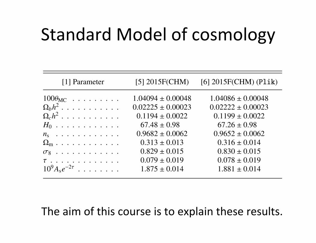
Standard'Model'of'cosmology'

hDp://arxiv.org/abs/1502.01589'

Standard'Model'of'cosmology'Planck Collaboration: Cosmological parameters

0.0216 0.0224 0.0232

�bh2

0.0

0.2

0.4

0.6

0.8

1.0

P/P

max

1.0405 1.0420 1.0435

100��

2.00 2.25 2.50 2.75

109As

0.05 0.10 0.15 0.20

�

0.24 0.28 0.32 0.36

�m

0.110 0.115 0.120 0.125

�ch2

0.0

0.2

0.4

0.6

0.8

1.0

P/P

max

0.94 0.96 0.98 1.00

ns

0.80 0.84 0.88 0.92

�8

5 10 15 20

zre

65.0 67.5 70.0 72.5

H0

Planck TT Planck TT,TE,EE Planck TT+lensing Planck TT,TE,EE+lensing Planck TT,TE,EE+lensing+BAO Planck TT+lowP

Fig. 7. Marginalized constraints on parameters of the base ⇤CDM model for various data combinations, excluding low multipolepolarization, compared to the Planck TT+lowP constraints.

WMAP polarization data are statistically consistent. The HFIpolarization maps have higher signal-to-noise than the LFI andcould, in principle, provide a third cross-check. However, at thetime of writing, we are not yet confident that systematics in theHFI maps at low multipoles (` <⇠ 20) are at negligible levels. Adiscussion of HFI polarization at low multipoles will thereforebe deferred pending the third Planck data release.

Given the di�culty of making accurate CMB polarizationmeasurements at low multipoles, it is useful to investigate otherways of constraining ⌧. Measurements of the temperature powerspectrum provide a highly accurate measurement of the ampli-tude Ase�2⌧. However, as shown in PCP13 CMB lensing breaksthe degeneracy between ⌧ and As. The observed Planck TT spec-trum is, of course, lensed, so the degeneracy between ⌧ and Asis partially broken when we fit models to the Planck TT likeli-hood. However, the degeneracy breaking is much stronger if wecombine the Planck TT likelihood with the Planck lensing like-lihood constructed from measurements of the power spectrum ofthe lensing potential C��` . The 2015 Planck TT and lensing like-lihoods are statistically more powerful than their 2013 counter-parts and the corresponding determination of ⌧ is more precise.The 2015 Planck lensing likelihood is summarized in Sec. 5.1and discussed in more detail in Planck Collaboration XV (2015).The constraints on ⌧ and zre

13 for various data combinations ex-cluding low multipole polarization data from Planck are summa-rized in Fig. 7 and compared with the baseline Planck TT+lowPparameters. This figure also shows the shifts of other parame-ters of the base ⇤CDM cosmology, illustrating their sensitivityto changes in ⌧.

13We use the same specific definition of zre as in the 2013 papers,where reionization is assumed to be relatively sharp with a mid-pointparameterized by a redshift zre and width �zre = 0.5. Unless otherwisestated we impose a flat prior on the optical depth with ⌧ > 0.01.

The Planck constraints on ⌧ and zre in the base⇤CDM modelfor various data combinations are:

⌧ = 0.078+0.019�0.019, zre = 9.9+1.8

�1.6, Planck TT+lowP; (17a)

⌧ = 0.070+0.024�0.024, zre = 9.0+2.5

�2.1, Planck TT+lensing; (17b)

⌧ = 0.066+0.016�0.016, zre = 8.8+1.7

�1.4, Planck TT+lowP (17c)+lensing;

⌧ = 0.067+0.016�0.016, zre = 8.9+1.7

�1.4, Planck TT+lensing (17d)+BAO;

⌧ = 0.066+0.013�0.013, zre = 8.8+1.3

�1.2, Planck TT+lowP (17e)+lensing+BAO.

The constraint from Planck TT+lensing+BAO on ⌧ is com-pletely independent of low multipole CMB polarization data andagrees well with the result from Planck polarization (and hascomparable precision). These results all indicate a lower redshiftof reionization than the value zre = 11.1± 1.1 derived in PCP13,based on the WMAP9 polarization likelihood. The low valuesof ⌧ from Planck are also consistent with the lower value of ⌧derived from the WMAP Planck 353 GHz-cleaned polarizationlikelihood, suggesting strongly that the WMAP9 value is biasedslightly high by residual polarized dust emission.

The Planck results of Eqs. (17a) – (17e) provide evidence fora lower optical depth and redshift of reionization than inferredfrom WMAP (Bennett et al. 2013), partially alleviating the dif-ficulties in reionizing the intergalactic medium using starlightfrom high redshift galaxies. A key goal of the Planck analysisover the next year is to assess whether these results are consis-tent with the HFI polarization data at low multipoles.

Given the consistency between the LFI and WMAP polariza-tion maps when both are cleaned with the HFI 353 GHz polariza-tion maps, we have also constructed a combined WMAP+Plancklow-multipole polarization likelihood (denoted lowP+WP). This

18

Standard'Model'of'cosmology'

The'aim'of'this'course'is'to'explain'these'results.'

Planck Collaboration: Cosmological parameters

Table 1. Parameters of the base ⇤CDM cosmology (as defined in PCP13) determined from the publicly released nominal-missionCamSpec DetSet likelihood [2013N(DS)] and the 2013 full-mission CamSpec DetSet and crossy-yearly (Y1 ⇥Y2) likelihoods withthe extended sky coverage [2013F(DS) and 2013F(CY)]. These three likelihoods are combined with the WMAP polarization like-lihood to constrain ⌧. The column labelled 2015F(CHM) lists parameters for a CamSpec cross-half-mission likelihood constructedfrom the 2015 maps using similar sky coverage to the 2013F(CY) likelihood (but greater sky coverage at 217 GHz and di↵erentpoint source masks, as discussed in the text). The column labelled 2015F(CHM) (Plik) lists parameters for the Plik cross-half-mission likelihood that uses identical sky coverage to the CamSpec likelihood. The 2015 temperature likelihoods are combinedwith the Planck lowP likelihood to constrain ⌧. The last two columns list the deviations of the Plik parameters from those ofthe nominal-mission and the CamSpec 2015(CHM) likelihoods. To help refer to specific columns, we have numbered the first sixexplicitly.

[1] Parameter [2] 2013N(DS) [3] 2013F(DS) [4] 2013F(CY) [5] 2015F(CHM) [6] 2015F(CHM) (Plik) ([2] � [6])/�[6] ([5] � [6])/�[5]

100✓MC . . . . . . . . . 1.04131 ± 0.00063 1.04126 ± 0.00047 1.04121 ± 0.00048 1.04094 ± 0.00048 1.04086 ± 0.00048 0.71 0.17⌦bh2 . . . . . . . . . . . 0.02205 ± 0.00028 0.02234 ± 0.00023 0.02230 ± 0.00023 0.02225 ± 0.00023 0.02222 ± 0.00023 �0.61 0.13⌦ch2 . . . . . . . . . . . 0.1199 ± 0.0027 0.1189 ± 0.0022 0.1188 ± 0.0022 0.1194 ± 0.0022 0.1199 ± 0.0022 0.00 �0.23H0 . . . . . . . . . . . . 67.3 ± 1.2 67.8 ± 1.0 67.8 ± 1.0 67.48 ± 0.98 67.26 ± 0.98 0.03 0.22ns . . . . . . . . . . . . 0.9603 ± 0.0073 0.9665 ± 0.0062 0.9655 ± 0.0062 0.9682 ± 0.0062 0.9652 ± 0.0062 �0.67 0.48⌦m . . . . . . . . . . . . 0.315 ± 0.017 0.308 ± 0.013 0.308 ± 0.013 0.313 ± 0.013 0.316 ± 0.014 �0.06 �0.23�8 . . . . . . . . . . . . 0.829 ± 0.012 0.831 ± 0.011 0.828 ± 0.012 0.829 ± 0.015 0.830 ± 0.015 �0.08 �0.07⌧ . . . . . . . . . . . . . 0.089 ± 0.013 0.096 ± 0.013 0.094 ± 0.013 0.079 ± 0.019 0.078 ± 0.019 0.85 0.05109Ase�2⌧ . . . . . . . . 1.836 ± 0.013 1.833 ± 0.011 1.831 ± 0.011 1.875 ± 0.014 1.881 ± 0.014 �3.46 �0.42

pixel-based likelihood that extends up to multipoles ` = 29. Useof the polarization information in this likelihood is denoted as“lowP” in this paper The optical depth inferred from the lowPlikelihood combined with the Planck TT likelihood is typically⌧ ⇡ 0.07, and is about 1� lower than the typical values of⌧ ⇡ 0.09 inferred from the WMAP polarization likelihood (seeSect. 3.4) used in the 2013 papers. As discussed in Sect. 3.4(and in more detail in Planck Collaboration XI 2015) the LFI70 GHz and WMAP polarization maps are consistent when bothare cleaned with the HFI 353 GHz polarization maps.7

(3) In the 2013 papers, the Planck temperature likelihood wasa hybrid: over the multipole range `= 2–49, the likelihoodwas based on the Commander algorithm applied to 94 % ofthe sky computed using a Blackwell-Rao estimator. The like-lihood at higher multipoles (`=50–2500) was constructed fromcross-spectra over the frequency range 100–217 GHz using theCamSpec software (Planck Collaboration XV 2014), which isbased on the methodology developed in (Efstathiou 2004) and(Efstathiou 2006). At each of the Planck HFI frequencies, thesky is observed by a number of detectors. For example, at217 GHz the sky is observed by four unpolarized spider-webbolometers (SWBs) and eight polarization sensitive bolometers(PSBs). The TOD from the 12 bolometers can be combined toproduce a single map at 217 GHz for any given period of time.Thus, we can produce 217 GHz maps for individual sky surveys(denoted S1, S2, S3, etc.), or by year (Y1, Y2) or split by half-mission (HM1, HM2). We can also produce a temperature mapfrom each SWB and a temperature and polarization map from

7Throughout this paper, we adopt the following labels for likeli-hoods: (i) Planck TT denotes the combination of the TT likelihood atmultipoles ` � 30 and a low-` temperature-only likelihood based onthe CMB map recovered with Commander; (ii) Planck TT+lowP fur-ther includes the Planck polarization data in the low-` likelihood, as de-scribed in the main text; (iii) labels such as Planck TE+lowP denote theT E likelihood at ` � 30 plus the polarization-only component of themap-based low-` Planck likelihood; and (iv) Planck TT,TE,EE+lowPdenotes the combination of the likelihood at ` � 30 using TT , T E,and EE spectra and the low-` temperature+polarization likelihood. Wemake occasional use of combinations of the polarization likelihoods at` � 30 and the temperature+polarization data at low-`, which we denotewith labels such as Planck TE+lowT,P.

quadruplets of PSBs. For example, at 217 GHz we produce fourtemperature and two temperature+polarization maps. We referto these maps as detectors-set maps (or “DetSets” for short);note that the DetSet maps can also be produced for any arbitrarytime period. The high multipole likelihood used in the 2013 pa-pers was computed by cross-correlating HFI DetSet maps forthe “nominal” Planck mission extending over 15.5 months.8 Forthe 2015 papers we use the full-mission Planck data extendingover 29 months for the HFI and 48 months for the LFI. In thePlanck 2015 analysis, we have produced cross-year and cross-half-mission likelihoods in addition to a DetSet likelihood. Thebaseline 2015 Planck temperature-polarization likelihood is alsoa hybrid, matching the high multipole likelihood at ` = 30 to thePlanck pixel-based likelihood at lower multipoles.

(4) The sky coverage used in the 2013 CamSpec likelihood wasintentionally conservative, retaining 58 % of the sky at 100 GHzand 37.3 % of the sky at 143 and 217 GHz. This was done toensure that on the first exposure of Planck cosmological resultsto the community, corrections for Galactic dust emission weredemonstrably small and had negligible impact on cosmologicalparameters. In the 2015 analysis we make more aggressive useof the sky at each of these frequencies. We have also tuned thepoint-source masks to each frequency, rather than using a sin-gle point-source mask constructed from the union of the pointsource catalogues at 100, 143, 217, and 353 GHz. This results inmany fewer point source holes in the 2015 analysis compared tothe 2013 analysis.

(5) Most of the results in this paper are derived from a revisedPlik likelihood based on cross half-mission spectra. The Pliklikelihood has been modified since 2013 so that it is now similarto the CamSpec likelihood used in PCP13. Both likelihoods usesimilar approximations to compute the covariance matrices. Themain di↵erence is in the treatment of Galactic dust correctionsin the analysis of the polarization spectra. The two likelihoodshave been written independently and give similar (but not iden-tical) results, as discussed further below. The Plik likelihood is

8Although we analysed a Planck full-mission temperature likeli-hood extensively prior to the release of the 2013 papers.

6

Planck Collaboration: Cosmological parameters

Table 1. Parameters of the base ⇤CDM cosmology (as defined in PCP13) determined from the publicly released nominal-missionCamSpec DetSet likelihood [2013N(DS)] and the 2013 full-mission CamSpec DetSet and crossy-yearly (Y1 ⇥Y2) likelihoods withthe extended sky coverage [2013F(DS) and 2013F(CY)]. These three likelihoods are combined with the WMAP polarization like-lihood to constrain ⌧. The column labelled 2015F(CHM) lists parameters for a CamSpec cross-half-mission likelihood constructedfrom the 2015 maps using similar sky coverage to the 2013F(CY) likelihood (but greater sky coverage at 217 GHz and di↵erentpoint source masks, as discussed in the text). The column labelled 2015F(CHM) (Plik) lists parameters for the Plik cross-half-mission likelihood that uses identical sky coverage to the CamSpec likelihood. The 2015 temperature likelihoods are combinedwith the Planck lowP likelihood to constrain ⌧. The last two columns list the deviations of the Plik parameters from those ofthe nominal-mission and the CamSpec 2015(CHM) likelihoods. To help refer to specific columns, we have numbered the first sixexplicitly.

[1] Parameter [2] 2013N(DS) [3] 2013F(DS) [4] 2013F(CY) [5] 2015F(CHM) [6] 2015F(CHM) (Plik) ([2] � [6])/�[6] ([5] � [6])/�[5]

100✓MC . . . . . . . . . 1.04131 ± 0.00063 1.04126 ± 0.00047 1.04121 ± 0.00048 1.04094 ± 0.00048 1.04086 ± 0.00048 0.71 0.17⌦bh2 . . . . . . . . . . . 0.02205 ± 0.00028 0.02234 ± 0.00023 0.02230 ± 0.00023 0.02225 ± 0.00023 0.02222 ± 0.00023 �0.61 0.13⌦ch2 . . . . . . . . . . . 0.1199 ± 0.0027 0.1189 ± 0.0022 0.1188 ± 0.0022 0.1194 ± 0.0022 0.1199 ± 0.0022 0.00 �0.23H0 . . . . . . . . . . . . 67.3 ± 1.2 67.8 ± 1.0 67.8 ± 1.0 67.48 ± 0.98 67.26 ± 0.98 0.03 0.22ns . . . . . . . . . . . . 0.9603 ± 0.0073 0.9665 ± 0.0062 0.9655 ± 0.0062 0.9682 ± 0.0062 0.9652 ± 0.0062 �0.67 0.48⌦m . . . . . . . . . . . . 0.315 ± 0.017 0.308 ± 0.013 0.308 ± 0.013 0.313 ± 0.013 0.316 ± 0.014 �0.06 �0.23�8 . . . . . . . . . . . . 0.829 ± 0.012 0.831 ± 0.011 0.828 ± 0.012 0.829 ± 0.015 0.830 ± 0.015 �0.08 �0.07⌧ . . . . . . . . . . . . . 0.089 ± 0.013 0.096 ± 0.013 0.094 ± 0.013 0.079 ± 0.019 0.078 ± 0.019 0.85 0.05109Ase�2⌧ . . . . . . . . 1.836 ± 0.013 1.833 ± 0.011 1.831 ± 0.011 1.875 ± 0.014 1.881 ± 0.014 �3.46 �0.42

pixel-based likelihood that extends up to multipoles ` = 29. Useof the polarization information in this likelihood is denoted as“lowP” in this paper The optical depth inferred from the lowPlikelihood combined with the Planck TT likelihood is typically⌧ ⇡ 0.07, and is about 1� lower than the typical values of⌧ ⇡ 0.09 inferred from the WMAP polarization likelihood (seeSect. 3.4) used in the 2013 papers. As discussed in Sect. 3.4(and in more detail in Planck Collaboration XI 2015) the LFI70 GHz and WMAP polarization maps are consistent when bothare cleaned with the HFI 353 GHz polarization maps.7

(3) In the 2013 papers, the Planck temperature likelihood wasa hybrid: over the multipole range `= 2–49, the likelihoodwas based on the Commander algorithm applied to 94 % ofthe sky computed using a Blackwell-Rao estimator. The like-lihood at higher multipoles (`=50–2500) was constructed fromcross-spectra over the frequency range 100–217 GHz using theCamSpec software (Planck Collaboration XV 2014), which isbased on the methodology developed in (Efstathiou 2004) and(Efstathiou 2006). At each of the Planck HFI frequencies, thesky is observed by a number of detectors. For example, at217 GHz the sky is observed by four unpolarized spider-webbolometers (SWBs) and eight polarization sensitive bolometers(PSBs). The TOD from the 12 bolometers can be combined toproduce a single map at 217 GHz for any given period of time.Thus, we can produce 217 GHz maps for individual sky surveys(denoted S1, S2, S3, etc.), or by year (Y1, Y2) or split by half-mission (HM1, HM2). We can also produce a temperature mapfrom each SWB and a temperature and polarization map from

7Throughout this paper, we adopt the following labels for likeli-hoods: (i) Planck TT denotes the combination of the TT likelihood atmultipoles ` � 30 and a low-` temperature-only likelihood based onthe CMB map recovered with Commander; (ii) Planck TT+lowP fur-ther includes the Planck polarization data in the low-` likelihood, as de-scribed in the main text; (iii) labels such as Planck TE+lowP denote theT E likelihood at ` � 30 plus the polarization-only component of themap-based low-` Planck likelihood; and (iv) Planck TT,TE,EE+lowPdenotes the combination of the likelihood at ` � 30 using TT , T E,and EE spectra and the low-` temperature+polarization likelihood. Wemake occasional use of combinations of the polarization likelihoods at` � 30 and the temperature+polarization data at low-`, which we denotewith labels such as Planck TE+lowT,P.

quadruplets of PSBs. For example, at 217 GHz we produce fourtemperature and two temperature+polarization maps. We referto these maps as detectors-set maps (or “DetSets” for short);note that the DetSet maps can also be produced for any arbitrarytime period. The high multipole likelihood used in the 2013 pa-pers was computed by cross-correlating HFI DetSet maps forthe “nominal” Planck mission extending over 15.5 months.8 Forthe 2015 papers we use the full-mission Planck data extendingover 29 months for the HFI and 48 months for the LFI. In thePlanck 2015 analysis, we have produced cross-year and cross-half-mission likelihoods in addition to a DetSet likelihood. Thebaseline 2015 Planck temperature-polarization likelihood is alsoa hybrid, matching the high multipole likelihood at ` = 30 to thePlanck pixel-based likelihood at lower multipoles.

(4) The sky coverage used in the 2013 CamSpec likelihood wasintentionally conservative, retaining 58 % of the sky at 100 GHzand 37.3 % of the sky at 143 and 217 GHz. This was done toensure that on the first exposure of Planck cosmological resultsto the community, corrections for Galactic dust emission weredemonstrably small and had negligible impact on cosmologicalparameters. In the 2015 analysis we make more aggressive useof the sky at each of these frequencies. We have also tuned thepoint-source masks to each frequency, rather than using a sin-gle point-source mask constructed from the union of the pointsource catalogues at 100, 143, 217, and 353 GHz. This results inmany fewer point source holes in the 2015 analysis compared tothe 2013 analysis.

(5) Most of the results in this paper are derived from a revisedPlik likelihood based on cross half-mission spectra. The Pliklikelihood has been modified since 2013 so that it is now similarto the CamSpec likelihood used in PCP13. Both likelihoods usesimilar approximations to compute the covariance matrices. Themain di↵erence is in the treatment of Galactic dust correctionsin the analysis of the polarization spectra. The two likelihoodshave been written independently and give similar (but not iden-tical) results, as discussed further below. The Plik likelihood is

8Although we analysed a Planck full-mission temperature likeli-hood extensively prior to the release of the 2013 papers.

6

Let’s'get'started…'

Basic'principles'

The'Universe'is'enormous'and'we'can'observe'only'a'single'one…''We' cannot' carry' out' experiments' to' test' our' ideas:' we' use' our' knowledge' of'terrestrial'(or'solar'system)'physics'to'interpret'our'observa.ons.'This'can'lead'to'metaphysical' considera.ons.' Only' in' the' past' 60' years' has' cosmology' been'considered'a'“real”'science.''All'we'observe'is'the'twoZdimensional'sky:'the'radial'direc.on'is'a'combina.on'of'distance'and'.me'into'the'past.'''A'cri.cal'aspect'is'the'establishment'of'a'distance'ladder'than'can'be'extended'to'cosmological' scales.' This'work' started' in'earnest'with' the'work'of'Hubble,' and'con.nues'to'the'present'day'with'the'Gaia'satellite.''Suppor.ng'informa.on'may'come'from'the'ages'of'old'stars,'meteorites,'etc.'

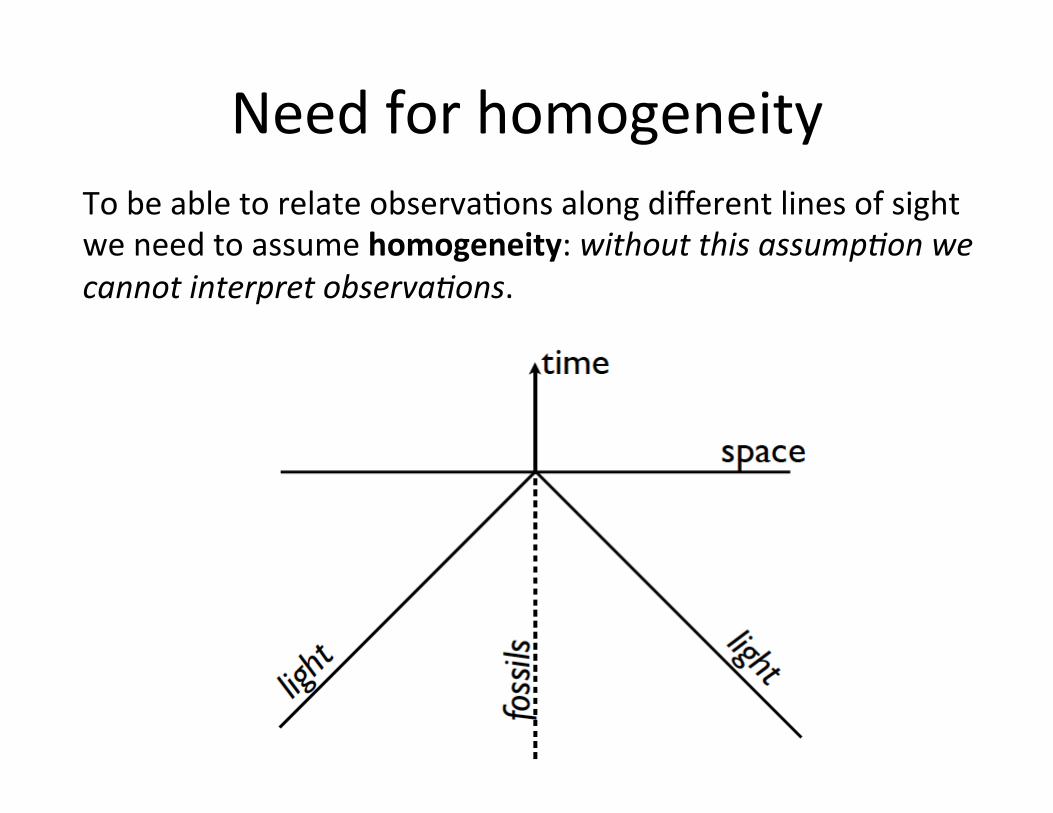
Need'for'homogeneity'To'be'able'to'relate'observa.ons'along'different'lines'of'sight'we'need'to'assume'homogeneity:'without+this+assump0on+we+cannot+interpret+observa0ons.'

Homogeneity'and'Isotropy'Homogeneity:'the'Universe'looks'the'same'at'each'point.'Isotropy:'the'Universe'looks'the'same'in'all'direc.ons.''Homogeneity'does'not'imply'isotropy,'and'isotropy'does'not'imply'homogeneity.'

Copernican'Principle'

The'Earth'is'not'a'special'place'in'the'Universe''(or:'we'are'not'privileged'observers).''This'is'a'major'shin'from'the'Ptolemaic'system'that'formed'the'basis'of'medieval'cosmology.''This'implies'that'the'Universe'is'isotropic'about'every'point,'which'implies'homogeneity'as'well.'

Cosmological'Principle'

The'cosmological'principle:''the'Universe'is'homogeneous'and+isotropic.'

‘Perfect’'Cosmological'Principle:''

Z  “The'universe'is'the'same'in'all'places,'direc.ons'and'.mes'

Z  This'mo.vated'the'‘SteadyZState’'universe'(Bondi,'Gold,'Hoyle)'

In'fact'it'does'not'apply'–'the'Universe'evolves'(as'we'shall'see).'

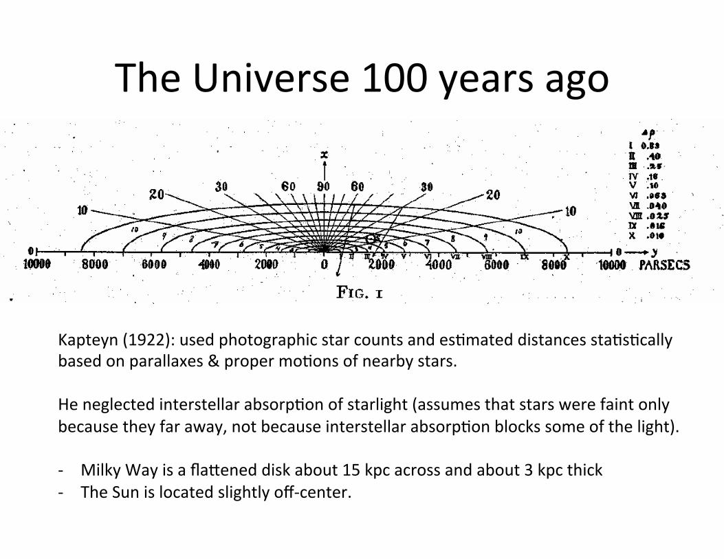
The'Universe'100'years'ago'

Kapteyn'(1922):'used'photographic'star'counts'and'es.mated'distances'sta.s.cally'

based'on'parallaxes'&'proper'mo.ons'of'nearby'stars.''

'

He'neglected'interstellar'absorp.on'of'starlight'(assumes'that'stars'were'faint'only'

because'they'far'away,'not'because'interstellar'absorp.on'blocks'some'of'the'light).'

'

Z  Milky'Way'is'a'flaDened'disk'about'15'kpc'across'and'about'3'kpc'thick''

Z  The'Sun'is'located'slightly'offZcenter.''

Shapley’s'Universe'Shapley's'Results'(1921):''''''Globular'clusters'form'a'subsystem'centered'on'the'Milky'Way.'''''The'Sun'is'16'kpc'from'the'MW'center.'''''MW'is'a'flaDened'disk'about'100'kpc'across'''Right'basic'result,'but'too'big:''''''Shapley'ignored'interstellar'absorp.on'''''Caused'him'to'overes.mate'the'distances'

Distances'to'other'galaxies'

At'the'same'.me'there'was'an'ongoing'discussion'about'the'nature'of'the'“nebulae”:'are'they'part'of'our'Galaxy'or'“island'Universes”.''Technology'came'to'the'rescue'thanks'to'the'construc.on'of'the'100Zinch'(2.5'm)'Hooker'telescope,'which'allowed'Hubble'to'iden.fy'Cepheid'variables'in'nearby'galaxies.''He'showed'that'the'“nebulae”'are'not'part'of'the'Milky'Way.'By'combining'his'distances'with'redshin'measurements'by'Slipher'and'Humason'he'found'that:'

VelocityZDistance'diagram'

Hubble'(1929):'the'recession'velocity'is'propor.onal'to'the'distance'(aner'allowing'for'the'Sun’s'mo.on):'v'='H0'r.+'Hubble'obtained'H0'=464'km/s/Mpc.'

Implica.on'of'Hubble’s'discovery'

At'first'glance,'this'result'may'violate'the'Copernican'Principle,'but'this'is'in'fact'not'true!'''''

The'recession'velocity'is'symmetric:'if'A'sees'B'receding,'then'B'sees'that'A'is'receding.'The'diagrams'from'the'two'different'points'of'view'are'iden.cal'except'for'the'names'of'the'galaxies.'

Implica.on'of'Hubble’s'discovery'The'linear'rela.on'is'the'only'one'consistent'with'the'Copernican'Principle.'For'e.g.'a'quadra.c'rela.on'different'observers'would'see'different'rela.ons.''

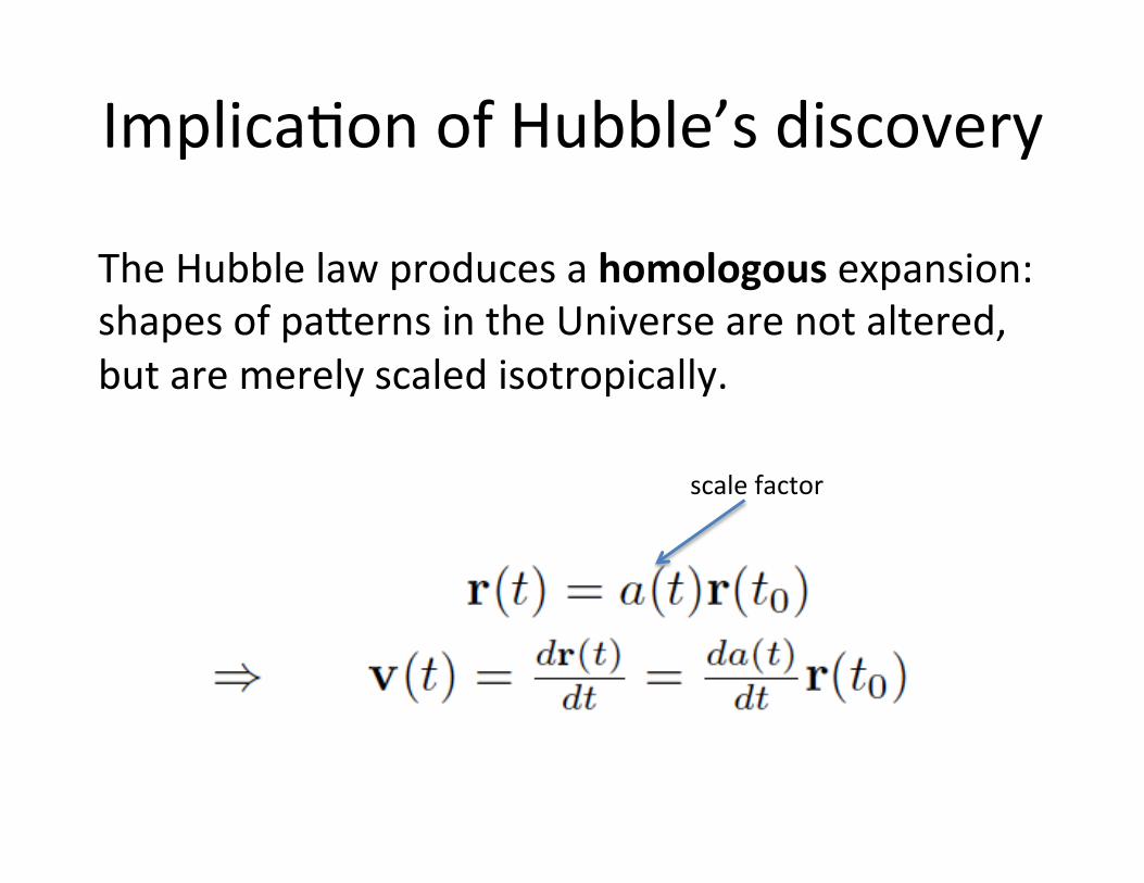
Implica.on'of'Hubble’s'discovery'

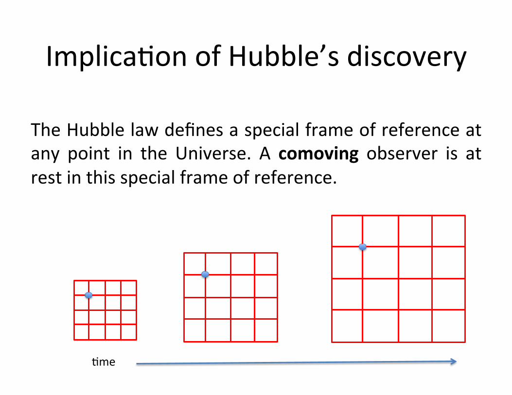
The'Hubble'law'produces'a'homologous'expansion:'shapes'of'paDerns'in'the'Universe'are'not'altered,'but'are'merely'scaled'isotropically.'

scale'factor'

Implica.on'of'Hubble’s'discovery'

The'Hubble'law'defines'a'special'frame'of'reference'at'any' point' in' the' Universe.' A' comoving' observer' is' at'rest'in'this'special'frame'of'reference.'

.me'

Age'of'the'Universe'

Note'that'the'Hubble'constant'has'dimension'1/.me:''1/H0=(978'Gyr)/(H0'in'km/s/Mpc)''If'the'expansion'velocity'is'constant'then'all'galaxies'were'in'the'same'place't=1/H0'years'ago.'With'the'current'es.mates'of'H0=71±3'km/s'this'implies'an'age'of'14'Gyr.''The'expansion'rate'is'not'a'constant,'so'the'result'is'only'an'indica.on:'typically'the'age'of'the'Universe'is'<1/H0.''Similarly'c/H0'is'a'natural'scale'for'the'Universe.'

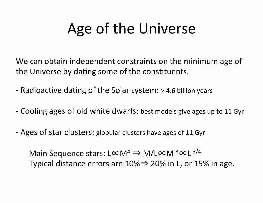
Age'of'the'Universe'

We'can'obtain'independent'constraints'on'the'minimum'age'of'

the'Universe'by'da.ng'some'of'the'cons.tuents.'

'

Z'Radioac.ve'da.ng'of'the'Solar'system:'>'4.6'billion'years'

'

Z'Cooling'ages'of'old'white'dwarfs:'best'models'give'ages'up'to'11'Gyr'

'

Z'Ages'of'star'clusters:'globular'clusters'have'ages'of'11'Gyr'

'

'Main'Sequence'stars:'L�M4'�'M/L�MZ3�LZ3/4'

'Typical'distance'errors'are'10%�'20%'in'L,'or'15%'in'age.''

Implica.on'of'Hubble’s'discovery'

The'Hubble'law'defines'a'special'frame'of'reference'at'any' point' in' the' Universe.' A' comoving' observer' is' at'rest'in'this'special'frame'of'reference.'

.me'

Reaching'the'Hubble'flow'

Our'Solar'System'is'not'quite'comoving:'it'moves'with'a'peculiar'velocity'of'370'km/s'rela.ve'to'the'observable'Universe.'''The' Local'Group'of' galaxies,'which' includes' the'Milky'Way,' appears' to' be'moving' at' 600' km/sec' rela.ve' to'the'observable'Universe.''''

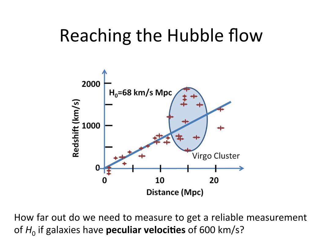
Reaching'the'Hubble'flow'

How'far'out'do'we'need'to'measure'to'get'a'reliable'measurement'of'H0'if'galaxies'have'peculiar'veloci>es'of'600'km/s?'

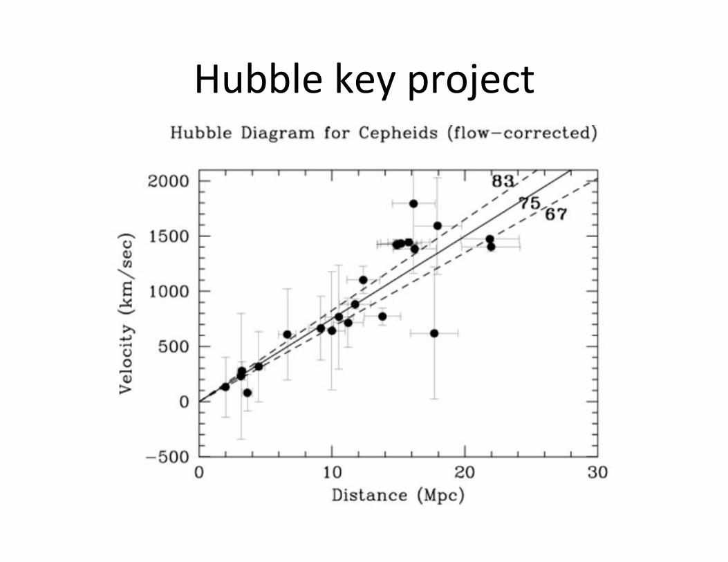
Hubble'key'project'

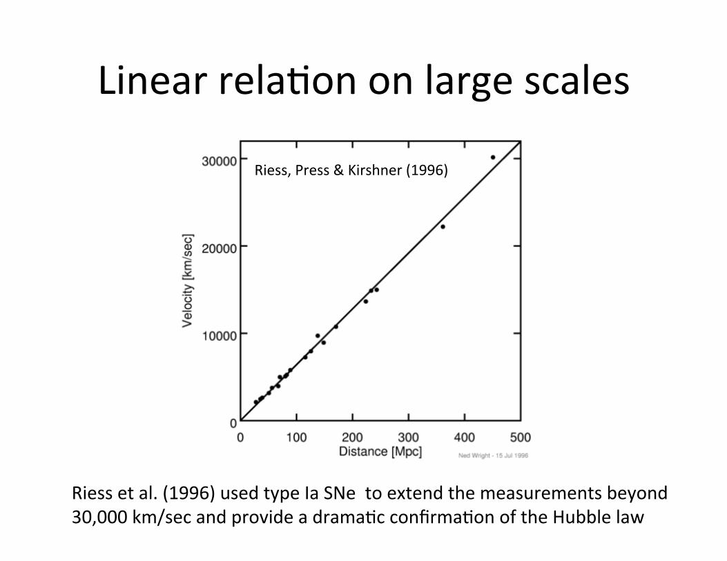
Linear'rela.on'on'large'scales'

Riess,'Press'&'Kirshner'(1996)'

Riess'et'al.'(1996)'used'type'Ia'SNe''to'extend'the'measurements'beyond'30,000'km/sec'and'provide'a'drama.c'confirma.on'of'the'Hubble'law'

Linear'rela.on'on'large'scales'

Type'Ia'SNe''allow'us'to'extend'the'measurements'beyond'30,000'km/sec'and'provide'a'drama.c'confirma.on'of'the'Hubble'law'

Evolving'Universe!'

The'posi.ve'value'for'H0'implies'the'Universe'is'expanding,'which'is'a'natural'consequence'of'General'Rela.vity.''The'Universe'was'smaller'in'the'past,'and'the'physical'condi.ons'must'have'differed;'observa.ons'of'distant'objects'show'a'different'epoch.''The+Universe+is+evolving.+

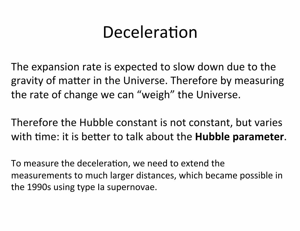
Decelera.on'

The'expansion'rate'is'expected'to'slow'down'due'to'the'gravity'of'maDer'in'the'Universe.'Therefore'by'measuring'the'rate'of'change'we'can'“weigh”'the'Universe.'''Therefore'the'Hubble'constant'is'not'constant,'but'varies'with'.me:'it'is'beDer'to'talk'about'the'Hubble'parameter.''To'measure'the'decelera.on,'we'need'to'extend'the'measurements'to'much'larger'distances,'which'became'possible'in'the'1990s'using'type'Ia'supernovae.'

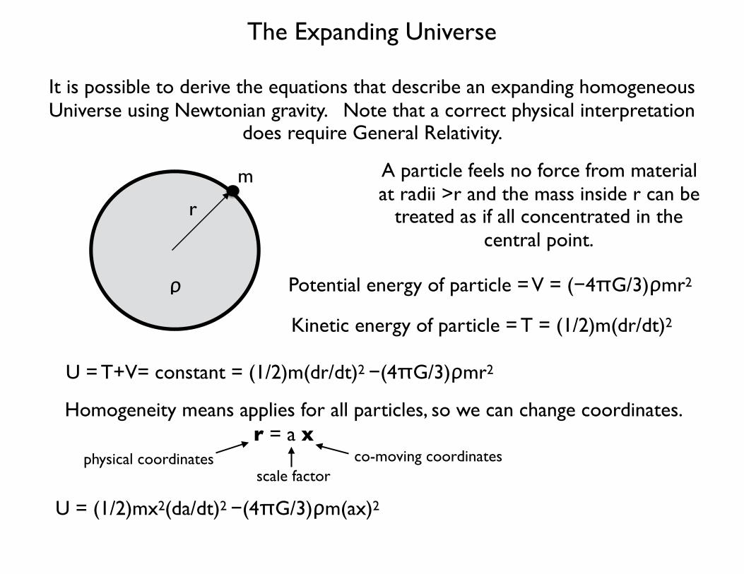
The Expanding Universe

It is possible to derive the equations that describe an expanding homogeneous Universe using Newtonian gravity. Note that a correct physical interpretation

does require General Relativity.

A particle feels no force from material at radii >r and the mass inside r can be

treated as if all concentrated in the central point.

r

ρ Potential energy of particle = V = (−4πG/3)ρmr2

m

Kinetic energy of particle = T = (1/2)m(dr/dt)2

U = T+V= constant = (1/2)m(dr/dt)2 −(4πG/3)ρmr2

Homogeneity means applies for all particles, so we can change coordinates.r = a x

co-moving coordinatesphysical coordinatesscale factor

U = (1/2)mx2(da/dt)2 −(4πG/3)ρm(ax)2

The Expanding Universe

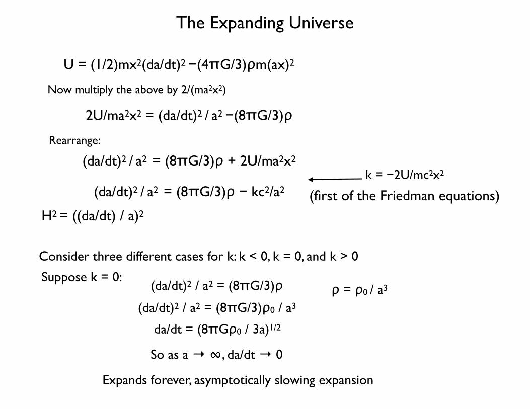
U = (1/2)mx2(da/dt)2 −(4πG/3)ρm(ax)2

Now multiply the above by 2/(ma2x2)

2U/ma2x2 = (da/dt)2 / a2 −(8πG/3)ρ

(da/dt)2 / a2 = (8πG/3)ρ + 2U/ma2x2

Rearrange:

k = −2U/mc2x2

(da/dt)2 / a2 = (8πG/3)ρ − kc2/a2

Consider three different cases for k: k < 0, k = 0, and k > 0

H2 = ((da/dt) / a)2

Suppose k = 0:(da/dt)2 / a2 = (8πG/3)ρ ρ = ρ0 / a3

(da/dt)2 / a2 = (8πG/3)ρ0 / a3

da/dt = (8πGρ0 / 3a)1/2

So as a → ∞, da/dt → 0

(first of the Friedman equations)

Expands forever, asymptotically slowing expansion

The Expanding Universe

Suppose k < 0:(da/dt)2 / a2 = (8πG/3)ρ − kc2/a2

As a → ∞,

small

(da/dt)2 = |k|c2

Suppose k > 0:

(da/dt)2/a2 = (8πG/3)ρ − kc2/a2

a = (3kc2/8πGρ)1/2

So eventually expansion will stop and da/dt = 0, so

d2a/dt2 = (1/2(da/dt))(−8πGρ0 / 3a2)(da/dt)) = −4πGρ0 / 3a2 < 0

da/dt = (8πGρ0 / 3a - kc2)1/2

Expands forever, asymptotically slowing expansion

(8πG/3)ρ0/a3 − kc2/a2

As a → ∞, first term grow slower than second

(8πG/3)ρ0/a3 − kc2/a2 = 0

Let’s look at how the evolution of the scale factor proceeds

Expansion stops… turns around such that the universe recollapses…

The'fate'of'the'Universe'

What'sets'the'value'of'k?'

The Expanding Universe

Suppose k = 0:da/dt = (8πGρ0 / 3a)1/2

da a1/2= (8πGρ0 / 3)1/2 dt

(2/3)a3/2 = (8πGρ0 / 3)1/2 ta = t2/3 (6πGρ0)1/2

a = (t/t0)2/3

Note that H = (da/dt)/a = (2/3)(t/t0)−1/3 / (t/t0)2/3 = 2/3 (1/t0)

t0 = 2/(3H0)

∫da a1/2 = ∫(8πGρ0 / 3)1/2 dt

If we take t0 = (1/6πGρ0)1/2, then

As such, the scale factor a equals 1 at the present day t0

Note that the k = 0 is between the k < 0 and k > 0 cases and hence represents the critical density.

H2 = (da/dt)2/a2 = (8πG/3)ρcrit

ρcrit = 3H2 / (8πG) ρcrit,0 = 3H02 / (8πG)

The Expanding Universe

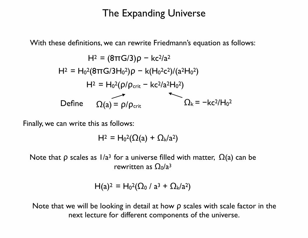
With these definitions, we can rewrite Friedmann’s equation as follows:

H2 = (8πG/3)ρ − kc2/a2

H2 = H02(ρ/ρcrit − kc2/a2H02)

H2 = H02(8πG/3H02)ρ − k(H02c2)/(a2H02)

H2 = H02(Ω(a) + Ωk/a2)

Ωk = −kc2/H02Ω(a) = ρ/ρcritDefine

Finally, we can write this as follows:

H(a)2 = H02(Ω0 / a3 + Ωk/a2)

Note that ρ scales as 1/a3 for a universe filled with matter, Ω(a) can be rewritten as Ω0/a3

Note that we will be looking in detail at how ρ scales with scale factor in the next lecture for different components of the universe.

Decelera.on'

The'expansion'rate'is'expected'to'slow'down'due'to'the'gravity'of'maDer'in'the'Universe.'Therefore'by'measuring'the'rate'of'change'we'can'“weigh”'the'Universe.'''Therefore'the'Hubble'constant'is'not'constant,'but'varies'with'.me:'it'is'beDer'to'talk'about'the'Hubble'parameter.''To'measure'the'decelera.on,'we'need'to'extend'the'measurements'to'much'larger'distances,'which'became'possible'in'the'1990s'using'type'Ia'supernovae.'

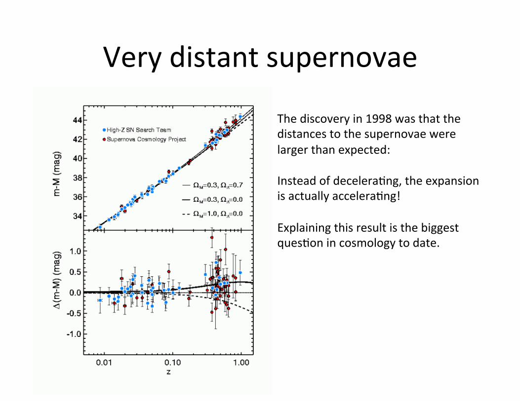
Very'distant'supernovae'

The'discovery'in'1998'was'that'the'distances'to'the'supernovae'were'larger'than'expected:''Instead'of'decelera.ng,'the'expansion'is'actually'accelera.ng!''Explaining'this'result'is'the'biggest'ques.on'in'cosmology'to'date.'