orlov spectra as a filtered cohomology theory · the orlov spectrum compares the generation times...

Available online at www.sciencedirect.com

Advances in Mathematics 243 (2013) 232–261www.elsevier.com/locate/aim

Orlov spectra as a filtered cohomology theory✩

Ludmil Katzarkova,b, Gabriel Kerra,∗

a Department of Mathematics, University of Miami, Coral Gables, FL, 33146, USAb Fakultat fur Mathematik, Universitat Wien, 1090 Wien, Austria

Received 7 November 2012; accepted 3 April 2013Available online 23 May 2013

Communicated by Tony Pantev

Abstract

This paper presents a new approach to the dimension theory of triangulated categories by consideringinvariants that arise in the pretriangulated setting.c⃝ 2013 The Authors. Published by Elsevier Inc. All rights reserved.

Keywords: Differential graded categories; Homological dimension; Triangulated categories; A-infinity modules

1. Introduction

In [17], Rouquier gave several results on the dimension theory of triangulated categories.Following this paper, Orlov computed the dimension of the derived category of coherent sheaveson an arbitrary smooth curve and found it to equal one in [16]. Orlov then advanced a moregeneral perspective on dimension theory by defining the spectrum of a triangulated category,now called the Orlov spectrum, which includes the generation times of all strong generators.The relevance of strong generators in triangulated categories and their connection to algebraicgeometry was thoroughly established in the seminal paper [3] by Bondal and Van den Bergh. Asthe Orlov spectrum compares the generation times amongst all strong generators, it serves as amore nuanced invariant than dimension.

In the important recent work [1] of Ballard, Favero and Katzarkov, gaps in the Orlov spectrumwere found to depend on the existence of algebraic cycles. To further this line of reasoning,

✩ This is an open-access article distributed under the terms of the Creative Commons Attribution License, whichpermits unrestricted use, distribution, and reproduction in any medium, provided the original author and source arecredited.

∗ Corresponding author.E-mail address: [email protected] (G. Kerr).

0001-8708/$ - see front matter c⃝ 2013 The Authors. Published by Elsevier Inc. All rights reserved.http://dx.doi.org/10.1016/j.aim.2013.04.002

http://www.elsevier.com/locate/aim

http://dx.doi.org/10.1016/j.aim.2013.04.002

http://www.elsevier.com/locate/aim

mailto:[email protected]

http://dx.doi.org/10.1016/j.aim.2013.04.002

L. Katzarkov, G. Kerr / Advances in Mathematics 243 (2013) 232–261 233

they stated the following conjectures which link large gaps in the Orlov spectrum to birationalinvariants.

Conjecture 1.1. Let X be a smooth algebraic variety. If ⟨A1, . . . ,An⟩ is a semi-orthogonaldecomposition of T , then the length of any gap in Db(X) is at most the maximal Rouquierdimension amongst the Ai .

Conjecture 1.2. Let X be a smooth algebraic variety. If A is an admissible subcategory ofDb(X), then the length of any gap of A is at most the maximal length of any gap of Db(X).Conversely, if A has a gap of length at least s, then so does Db(X).

These have many important corollaries connecting birational geometry to triangulated cate-gories and their Orlov spectrum. We recall again from [1] two such results.

Corollary 1.3. Suppose Conjectures 1.1 and 1.2 hold. Let X and Y be birational smooth propervarieties of dimension n. The category, Db(X), has a gap of length n or n − 1 if and only ifDb(Y ) has a gap of the same length i.e. the gaps of length greater than n − 2 are a birationalinvariant.

Corollary 1.4. Suppose Conjectures 1.1 and 1.2 hold. If X is a rational variety of dimension n,then any gap in Db(X) has length at most n − 2.

Establishing a procedure for computing the Orlov spectrum of Db(X) would also allow us topursue, for example, the following.

Conjecture 1.5. Let X be a generic smooth four dimensional cubic. Then the gap of the spectraof the derived category of this cubic is equal to two.

From the considerations above, this conjecture implies that generic smooth four dimensionalcubic is not rational, a standing question in algebraic geometry.

While the triangulated setting serves as an accessible model for homological invariants, it isgenerally accepted that triangulated categories are inadequate for giving a natural characteriza-tion of homotopy theory for derived categories. Instead of working in this setting, it is advisableto lift to a pretriangulated category, or (∞, 1)-category framework, where several constructionsare more natural [15,7]. In this paper, we study the Orlov spectra of triangulated categories bylifting to pretriangulated DG or A∞-categories.

When the category T is strongly generated by a compact object G, we upgrade several clas-sical results in dimension theory of abelian categories to the pretriangulated setting and find thatthe natural filtration given by the bar construction plays a determining role in the calculus ofdimension. Indeed, if G is such a generator, using a result of Lefevre-Hasegawa, we can regardT as the homotopy category of perfect modules over an A∞ algebra AG = Hom∗(G,G). Inaddition to being a DG category, the category of perfect A∞ modules over AG is enhanced overfiltered chain complexes, where the filtration is obtained through the bar construction. This filtra-tion descends to the triangulated level. The first main result, Theorem 3.12, in this paper is thatthe generation time of a strong generator G equals the maximal length of this filtration.

Theorem 1.6. The generation time of G ∈ T equals the supremum over all M, N ∈ AG-mod∞

of the lengths of HomAG -mod∞(M, N ) with respect to the filtration induced by the bar

construction.

As a result, we develop a filtered cohomology theory which yields the generation times thatoccur in Orlov spectra. The lengths referred to in this theorem are those of the filtrations induced

234 L. Katzarkov, G. Kerr / Advances in Mathematics 243 (2013) 232–261

on the cohomology of the complexes, or the Ext groups, by the pretriangulated filtrations. Inpractice, it is possible to compute these lengths by calculating their spectral sequences whichwill converge under very mild assumptions.

Another filtration that occurs naturally from the bar construction is on the tensor product. Thisfiltration is especially useful as one may define change of base as a tensor product with an ap-propriate bimodule. After establishing basic adjunction results in the next section, we generalizethe classical change of base formula for dimension to the A∞ algebra setting in Theorem 3.20.A new multiplicative constant appears in this version which is related to the speed at which aspectral sequence associated to the tensor product filtration converges.

Theorem 1.7. Let P be a (B, A)-bimodule and M a left A-module. Suppose the spectral se-

quence of P∞

⊗A M degenerates at the (s + 1)-st page. If the convolution functor P∞

⊗ is faithful,then

lvlA(M) ≤ lvlA(P)+ s · lvlB(P∞

⊗A M).

Here lvlA(M) plays the role of homological, or projective, dimension of a module M . If thealgebra A is formal, the constant s is 1 and we see the classical formula. If higher products arerelevant, one must modify the classical inequality.

2. A∞ constructions

This section will review many definitions and constructions related to A∞ algebras and mod-ules. The aim of our treatment is to approach this subject with a special emphasis on the filtrationsarising from the bar constructions. These filtrations are the main technical structure we use in thedimension theory for pretriangulated categories.

After reviewing some standard definitions, we will give the definitions of filtered tensor prod-uct, filtered internal Hom and duals in the category of A∞-bimodules. The mantra that all con-structions in the A∞ setting are derived constructions will be continually reinforced. Moreover,the above functors will land in the category of lattice filtered A∞-modules, which preserves therelevant data for a study of dimension. The ⊗ − Hom adjunction, usually written in either theabelian or derived setting, will be formed as an adjunction between filtered DG functors. The cat-egorical formulation of this statement is that the category Alg∞ is a biclosed bicategory enrichedover filtered cochain complexes. We will utilize this to update classical results on the relationshipbetween flat and projective dimensions for perfect modules.

2.1. Fundamental notions

We take a moment to lay out some basic notation and fix our sign conventions. All algebrasand vector spaces will be over a fixed field K and categories will be K-linear categories. Letgr be the category of graded vector spaces over K and finite sums of homogeneous maps. Wetake Ch to be the category of cochain complexes of vector spaces over K and finite sums ofhomogeneous maps. We will identify HomCh with the internal Hom whose differential of

f ∈ HomkCh((C, dC ), (C

′, dC ′))

is the usual one, namely,

d f := f ◦ dC − (−1)kdC ′ ◦ f.

Finally, we take K to be the category of chain complexes and cochain maps. In other words,maps which are cocycles relative to d in Ch. For most of the paper, we will assume our chain


complexes are Z-graded, but there will be examples of the (Z/2Z)-graded case. This shouldcause no difficulty as the proofs will be independent of this choice.

We view Ch as a closed category with respect to the tensor product along with the Koszulsign rule γV,W : V ⊗ W → W ⊗ V given by:

γV,W (v ⊗ w) = (−1)|v||w|w ⊗ v. (2.1)

We will need to implement this sign convention when discussing tensor products of mapsas well. For this we follow the usual convention. Namely, given homogeneous maps f ∈

Hom∗gr (V1, V2) g ∈ Hom∗

gr (W1,W2) then we define f ⊗ g ∈ Homgr (V1 ⊗ W1, V2 ⊗ W2)

via ( f ⊗ g)(v ⊗ w) = (−1)|g||v| f (v)⊗ g(w).

By a differential graded, or DG, category D we mean a category enriched in Ch. We let

h : D → ChDop

be the Yoneda functor given by hE (E ′) = HomD(E ′, E).

In categories gr , Ch and K , we have the shift functor s which sends V ∗ to V ∗+1. On mor-phisms we have s( f ) = (−1)| f | f . There is also a (degree 1) natural transformation σ : I → sdefined as σ(v) = (−1)|v|v. One can utilize σ to translate the signs occurring in various bar con-structions given in this text and those in the ordinary desuspended case. In particular, given a mapf : V ⊗n

→ W ⊗m in Ch we define s⊗( f ) : (sV )⊗n→ (sW )⊗m to be σ⊗m

◦ f ◦ (σ−1)⊗n . Wewill often use this notation to write the equations defining various structures without mentioningthe elements of our algebras or modules. A nice account of the various choices and techniquesused in sign conventions can be found in [6].

Filtrations will occur throughout this paper and our initial approach will be rather general. Wepartially order Zk for any k ∈ N with the product order. A lattice filtered complex will consistof the data V =

V, {Vα}α∈Zk

for some k ∈ N, where V is an object in Ch and {Vα}α∈Zk is a

collection of subcomplexes partially ordered by inclusion. If k = 1, we simply call V filtered.Given two lattice filtered complexes V =

V, {Vα}α∈Zk

and W =

W, {Wβ}β∈Zl

, we define

the lattice filtered tensor product and internal hom as follows.

V ⊗ W =V ⊗ W, {Vα ⊗ Wβ}(α,β)∈Zk+l

and

Hom (V,W) =

Hom (V,W ) , {Hom−α,β (V,W )}(α,β)∈Zk+l

where Hom−α,β (V,W ) = {φ : V → W |φ(Vα) ⊆ Wβ}. The category of lattice filtered com-plexes and filtered complexes will be denoted Chl f and Ch f respectively. We note that the aboveconstructions make Chl f a closed symmetric monoidal category.

Given a DG category D, we define the category Dl f to have objects consisting of the dataE =

E, {Eα}α∈Zk

where

hE (E ′), {(hEα (E

′))}α∈Zk

∈ Chl f for every object E ′∈ D. The

cochain complex of morphisms between D and E is simply HomD(D, E). Restricting to the caseof k = 1 yields the definition of D f .

The total filtration functor Tot : Chl f→ Ch f is defined as

TotV, {Vα}α∈Zk

=V, {∪|α|=n Vα}n∈Z


for k = 0 where |α| = a1 + · · · + ak for α = (a1, . . . , ak). One needs to deal with k = 0 a bitdifferently and define Tot (V, {V0}) =

V, {V ′

n}

with V ′n = 0 for n < 0 and V ′

n = V0 otherwise.Now suppose V ∈ Ch f is a filtered complex. Letting Zn be the subspace of cocycles in Vn ,

we have that the cohomology

H∗(V) =

H∗(V ),

H∗(V )n =

Zn

im(d) ∩ Zn

n∈Z

is then a filtered object in gr . We define the upper and lower length of the filtration as follows. If∪n H∗(V) = H∗(V ) we take ℓ+(V) = ∞ and if ∩n H∗(V) = 0 then ℓ−(V) = −∞. Otherwise,we define these lengths as

ℓ+(V) = inf{n : H∗(V )n = H∗(V )} ℓ−(V) = inf{n : H∗(V )n = 0}. (2.2)

By the length ℓ(V) of V we will mean the maximum of |ℓ+(V)| and |ℓ−(V)|. We extend thesedefinitions to V ∈ Chl f by taking length of Tot(V).

Given a DG category D and an object E ∈ Dl f , we define the lengths of E as

ℓ+(E) = sup{ℓ+(hE(E′)) : E ′

∈ D},

ℓ−(E) = inf{ℓ−(hE(E′)) : E ′

∈ D},

ℓ(E) = sup{ℓ(hE(E′)) : E ′

∈ D}.

Given two DG categories D, D, a DG functor F : D → D f and E ∈ D, we take ℓF±(E) =

ℓ±(F(E)) and ℓF= sup{ℓF (E) : E ∈ D}. One can consider ℓF as a generalization of the

cohomological dimension of a functor between abelian categories. Note that in the DG categoryCh the two notions of length are equal. In other words, the definition given by Eqs. (2.2) yieldthe same quantities as the definition above using the Yoneda embedding h .

A motivating example for the above definitions is the case where D and D are categories ofbounded below cochain complexes of injective objects in abelian categories D and D. Note thatthese categories admit embeddings into their filtered versions by sending any complex E∗ to(E∗, {τn(E∗)}n∈Z) where τn(E∗)k = Ek for k ≤ n and zero otherwise. Assuming D and D haveenough injectives, any functor F : D → D has the (pre)derived DG functor RF : D → D andafter composition with the embedding above one has a DG functor F : D → D f . It is then plainto see that ℓF equals the cohomological dimension of F .

2.2. A∞-algebras

One of the fundamental structures in our study is an A∞-algebra.

Definition 2.1. A non-unital A∞-algebra A is an object A ∈ Ch and a collection of degree 1maps µn

A : (s A)⊗n→ s A for n > 0 satisfying the relation

nk=0

n−kr=0

µn−k+1A ◦ (1⊗r

⊗ µkA ⊗ 1⊗(n−r−k))

= 0

for every n.

We note that it is common to see the definition utilizing the desuspended maps s−1⊗ (µn

A)whichinvolves more intricate signs.


In this paper we will assume that our A∞-algebras come equipped with a strict unit. We recallthat this means there exists a unit map u : K → A[1] where

µ2A(u ⊗ 1) = 1 = −µ2

A(1 ⊗ u) (2.3)

µn(1⊗r⊗ u ⊗ 1⊗(n−r−1)) = 0 for n = 2. (2.4)

We will normally write eA for u(1) (or e if the algebra is implicit).If A is an A∞-algebra, we take Aop to be the algebra with structure maps µk

Aop = µkA ◦ σk

where σk : (s A)⊗k→ (s A)⊗k reverses the ordering of the factors via the symmetric monoidal

transformation γ in Eq. (2.1).It is immediate that the cohomology H∗(A) defined with respect to µ1

A is a graded K-algebrawith multiplication induced by µ2

A. However, the higher products determine more structure thanthe cohomology algebra can express on its own. In order to see this we need to be able to comparetwo different algebras. A homomorphism of A∞-algebras is defined as follows.

Definition 2.2. If (A, µ∗

A) and (B, µ∗

B) are A∞-algebras then a collection of graded maps φn:

(s A)⊗n→ s B for n ≥ 1 is an A∞-map if

nk=1

n−kr=1

φn−k+1◦ (1⊗r

⊗ µkA ⊗ 1⊗(n−r−k))

=

nj=1

i1+···+i j =n

µjB ◦ (φ⊗i1 ⊗ · · · ⊗ φ⊗i j )

.A strictly unital homomorphism is also required to preserve the unit as well as satisfying the

identities

φr+s+1◦ (1⊗r

⊗ u ⊗ 1⊗s) = 0

for all r + s > 0. The category of unital and non-unital A∞-algebras will be denoted Alg∞ andAlgnu

∞ respectively.When all maps φk

= 0 except φ1, we call {φk} strict. If there is an A∞-map ϵA : A → K

we will call A augmented. Any augmented, strictly unital A∞ algebra is required to satisfy theequation ϵAu = 1K.

It is important to observe that [φ1] induces an algebra homomorphism H∗(A) to H∗(B) so

that cohomology is a functor from A∞-algebras to ordinary algebras. When the induced map [φ1]

is an isomorphism, we call φ∗ a quasi-isomorphism. The following proposition can be found inany of the basic references given above.

Proposition 2.3. Given a quasi-isomorphism φ∗: A → B there exists a quasi-isomorphismψ∗

:

B → A for which [φ1] and [ψ1

] are inverse.

Some of the A∞-algebras discussed in this paper satisfy additional conditions.

Definition 2.4. (i) An A∞-algebra is formal if it is quasi-isomorphic to its cohomology algebra.(ii) An A∞-algebra is compact if its cohomology algebra is finite dimensional.

While it is rarely the case that an A∞-algebra is formal, there is an A∞-structure on itscohomology, called the minimal model, which yields a quasi-isomorphic A∞-algebra. It is a


well known fact that, for (A, µ∗

A), this is a uniquely defined A∞-structure (H∗(A), µ∗

A) withµ1

A = 0 (here µ2A = [µ2

A] and the higher µ∗

A are determined by a tree level expansion formula).Let us state this as a proposition.

Proposition 2.5. For any A∞-algebra (A, µ∗

A) there is an A∞-algebra (H∗(A), µ∗

A), uniquelydefined up to A∞-isomorphism, and a quasi-isomorphism φA : A → H∗(A). We call (H∗(A),µ∗

A) a minimal model of (A, µ∗

A).

It will be important to have at our disposal another equivalent definition, the algebra bar con-struction, for which we closely follow [13,10]. First, given V ∈ gr we denote the tensor algebraand coalgebra by T a V and T cV respectively. As graded vector spaces, both are equal to

T V =

∞n=0

V ⊗n .

For space considerations, we will use bar notation and write [v1| · · · |vn], or simply v, for v1⊗· · ·⊗vn for an arbitrary element of T V . These spaces are bigraded, with one grading denotingthe length of a tensor product, and the other denoting the total degree. Our notation conventionsfor these gradings will be

(T V )r,s =

[v1| · · · |vr ] :

|vi | = s

.

In many situations, we will be interested only in the length grading, in which case we use thenotation

(T V )n = ⊕nk=0(T V )k,• (T V )>n = ⊕k>n(T V )k,•.

The algebra map for T a V is the usual product and the coalgebra map ∆ : T cV → T cV⊗K T cV is defined as

∆[v1| · · · |vn] =

ni=0

[v1| · · · |vi ] ⊗ [vi+1| · · · |vn]

where the empty bracket [] denotes the identity in K.The tensor coalgebra naturally lives in the category of coaugmented, counital, dg coalgebras

Cog′. The objects in this category consist of data (C, d, η, ϵ) where C is a coalgebra, d is adegree 1, square zero, coalgebra derivation, η : C → K and ϵ : K → C are the counit andcoaugmentation satisfying ηϵ = 1K. However, this category is too large for our purposes and weinstead consider a subcategory Cog consisting of cocomplete objects. To define these objects,take π : C → C = C/K to be the cokernel of ϵ. Consider the kernel Cn = ker(∆n) where

∆n: C

∆n

−→ C⊗n π⊗n

−→ C⊗n.

Elements of Cn are called n-primitive and C1 is referred to as the coaugmentation ideal. Theyform an increasing sequence

C0 ⊂ C1 ⊂ · · ·

called the canonical filtration.


This defines a natural inclusion Cog′→ (Cog′) f and we say that the augmented coalgebra C

is cocomplete if C = lim Cn . One easily observes that the tensor coalgebra is an object of Cog as

(T cV )n = (T V )n,•.

Moreover, the tensor coalgebra T cV is cofree in the category Cog (i.e. the tensor coalgebrafunctor is right adjoint to the forgetful functor).

Now we recall the (coaugmented) bar functor

B : Algnu∞ → Cog

which takes any non-unital A∞-algebra (A, µA) to B A = (T c(s A), bA, ηB A, ϵB A). The defi-nitions of the counit and coaugmentation are clear. We define bA : T c(s A) → T c(s A) via itsrestriction to (s A)⊗n as

bA|(s A)⊗n =

nk=1

n−kr=0

1⊗r⊗ µk

A ⊗ 1⊗(n−r−k)

.

There are several variants of this construction, most importantly the ordinary bar constructionB A = (T (s A)>0, bA) which takes values in cocomplete coalgebras. We fix notation for theinclusion to be

ιA : B A ↩→ B A. (2.5)

The differential is simply the restriction of the one defined in the coaugmented case. It is helpfulto understand B A when A is an ordinary algebra A. In this case, we see that B A is just theaugmented bar resolution for A (and hence, acyclic).

The bar construction of A inherits the increasing filtration

Bn A := ⊕i≤n(B A)i,• = (B A)n .

We refer to this, and the module variants to come, as the length filtration.

Remark 2.6. We note here that one advantage of the bar construction is the ease at which one candiscuss structures that are more difficult to define in the category Alg∞. One example of this isthe tensor product of two A∞-algebras A, A′ which has more than one fairly intricate definition.In Cog we define the tensor product of B A⊗B A′ in the usual way. We then say that B ∈ Alg∞ isquasi-isomorphic to the tensor product if B = A ⊗ A′ and B B is quasi-isomorphic to B A ⊗ B A′

in Cog f . See [14] for an article comparing various constructions of a natural quasi-isomorphism.

2.3. A∞ polymodules

We start this section with a general definition of a module over several A∞-algebras whichwe call a polymodule. It is both useful and correct to think of a polymodule as a bimodulewith respect to the tensor product of several algebras or, even more simply, as a module overthe tensor product of algebras and their opposites. This is analogous to defining an (R, S)bimodule as opposed to an R ⊗ Sop module. We take this approach at the outset to avoid someof the cumbersome notation and uniqueness issues surrounding the tensor product of multipleA∞-algebras. This is accomplished utilizing the bar construction and working in the category ofcomodules where many structures are more accessible. The definitions and results in this sectionare adaptations of those for modules and bimodules which can be found in [13]. We add the


caveat that Lefevre-Hasegawa uses the different term polymodules to define what we would calla module.

For this section, we fix A∞-algebras A1, . . . , Ar and B1, . . . , Bs and write (a, b) for the data(A1, . . . , Ar |B1, . . . , Bs). Let P be a graded vector space and write

B(a,b)P = B A1 ⊗ · · · ⊗ B Ar ⊗ P ⊗ B B1 ⊗ · · · ⊗ B Bs (2.6)

for the bar construction of P .When (a, b) is fixed or understood from the context, we simply write BP . We make a note

that BP is naturally an object of Chl f where the lattice is Zr+s and the filtration is induced bythe length filtrations on the bar constructions. Given any γ ∈ Zr+s , we denote the γ filteredpiece of BP by Bγ P . Observe also that BP is a cofree left comodule over the coalgebrasB Ai and a cofree right comodule over coalgebras B Bi where ∆i,P : BP → B Ai ⊗ BP and∆P, j : BP → BP ⊗ B B j are the comodule maps. These are defined by repeatedly applyingγ from Eq. (2.1) to permute the left factor of B Ai and right factor of B B j to the left and rightrespectively, after having applied their comultiplications. We take,

∆P = ∆P,s ◦ · · · ◦ ∆P,1 ◦ ∆r,P ◦ · · · ◦ ∆1,P

as the polymodule comultiplication from BP to B A1 ⊗ · · · ⊗ B Ar ⊗ BP ⊗ B B1 ⊗ · · · ⊗ B Bs .The differentials on each coalgebra tensor to define the differential d ′

P : BP → BP .

Definition 2.7. A non-unital (a, b) = (A1, . . . , Ar |B1, . . . , Bs) polymodule (P, µP ) is a gradedvector space P along with a degree 1 map

µP : B(a,b)P → P (2.7)

satisfying the equation

µP ◦ [(1B A1 ⊗ · · · ⊗ 1B Ar ⊗ µP ⊗ 1B B1 ⊗ · · · ⊗ 1B Bs ) ◦ ∆ + d ′

P ] = 0. (2.8)

We call the P a polymodule if µP satisfies the unital conditions for every i and j ,

µP ◦ (ϵB A1 ⊗ · · · ⊗ uB Ai ⊗ · · · ⊗ ϵB Ar ⊗ 1P ⊗ ϵB B1 ⊗ · · · ⊗ ϵB Br ) = 1P ,

µP ◦ (ϵB A1 ⊗ · · · ⊗ ϵB Ar ⊗ 1P ⊗ ϵB B1 ⊗ · · · ⊗ uB B j ⊗ · · · ⊗ ϵB Br ) = 1P ,

µP ◦ (ιA1 ⊗ · · · ⊗ uB Ai ⊗ · · · ⊗ ιAr ⊗ 1P ⊗ ιB1 ⊗ · · · ⊗ ιBr ) = 0,

µP ◦ (ιA1 ⊗ · · · ⊗ ιAr ⊗ 1P ⊗ ιB1 ⊗ · · · ⊗ uB B j ⊗ · · · ⊗ ιBr ) = 0,

where ϵ is the coaugmentation and ι the inclusion from Eq. (2.5).

A bimodule is a polymodule for which r = 1 = s. A left module is a bimodule for whichB1 = K and similarly, a right module is a bimodule for which A1 = K. A non-unital morphismfrom the polymodule P to P ′ is defined as any gr map φ : BP → P ′. The collection of thesemaps forms a complex Hom(a,b)-Modnu

∞(P, P ′) with differential defined as

dφ = φ ◦ (1B A1 ⊗ · · · ⊗ 1B Ar ⊗ µP ⊗ 1B B1 ⊗ · · · ⊗ 1B Bs ) ◦ ∆P

+φ ◦ d ′

P − (−1)|φ|µP ′ ◦ (1B A1 ⊗ · · · ⊗ 1B Ar ⊗ φ ⊗ 1B B1 ⊗ · · · ⊗ 1B Bs ) ◦ ∆P .

(2.9)

A morphism φ ∈ Hom(a,b)-Mod∞(P, P ′) is a non-unital morphism satisfying the unital condi-

tions

φ ◦ (1B A1 ⊗ · · · ⊗ uB Ai ⊗ · · · ⊗ 1B Ar ⊗ 1P ⊗ 1B B1 ⊗ · · · ⊗ 1B Br ) = 0,


φ ◦ (1B A1 ⊗ · · · ⊗ 1B Ar ⊗ 1P ⊗ 1B B1 ⊗ · · · ⊗ uB B j ⊗ · · · ⊗ 1B Br ) = 0.

The fact that Hom(a,b)-Mod∞(P, P ′) is indeed a subcomplex follows from the unital condition

on algebras and modules. A morphism φ ∈ Hom(a,b)-Mod∞(P, P ′) is called strict if φ|B>0 P

= 0. A homomorphism is defined to be a cocycle in this complex. A homomorphism φ forwhich φ|B0 P : P → P ′ is a quasi-isomorphism will be called a quasi-isomorphism. Given ψ ∈

Hom(a,b)-Mod∞(P ′, P ′′) we define composition as

ψφ = ψ ◦ (1B A1 ⊗ · · · ⊗ 1B Ar ⊗ φ ⊗ 1B B1 ⊗ · · · ⊗ 1B Bs ) ◦ ∆P .

It is a straightforward, albeit tedious check to see that these definitions make (a, b) polymod-ules into a DG category which we label (a, b)-Mod∞, or just Mod∞. We write H0(Mod∞)

(H∗(Mod∞)) for the zeroth (graded) cohomology category. The next proposition follows imme-diately from Remark 2.6 and the naturality of γ . A rigorous proof is omitted but can be assembledfrom results in [13].

Proposition 2.8. The category of filtered (a, b) = (A1, . . . , Ar |B1, . . . , Bs) polymodules isquasi-equivalent to the category of filtered left A1 ⊗ · · · ⊗ Ar ⊗ Bop

1 ⊗ · · · ⊗ Bops -modules.

From this, or from a direct argument, one obtains the following corollary which will be appliedoften implicitly.

Corollary 2.9. The category of filtered (A1, . . . , Ar |B1, . . . , Bs) polymodules is naturallyequivalent to the category of filtered (A1, . . . , Ar , Bop

1 , . . . , Bops |K) polymodules.

Following [4], we observe that Mod∞ is a pretriangulated category with sums and shiftsdefined in the obvious way and the natural cone construction cone(φ) given in the usual way.Namely, cone(φ) is the graded vector space P ⊕ s P ′ and its structure morphism is

µcone(φ) =

µP σ ◦ φ

0 µs P ′

.

Given (a, b) we let

U(a,b) = A1 ⊗ · · · ⊗ Ar ⊗ B1 ⊗ · · · ⊗ Bs

be the trivial polymodule whose structure map is induced by suspension, γ and the algebrastructure maps. A free polymodule is defined as a direct sum of copies of U(a,b) and a projectivepolymodule as a direct summand of a free polymodule. A projective polymodule will be calledfinitely generated if it is a submodule of a finite sum of copies of U(a,b).

Definition 2.10. The subcategory of perfect (a, b) polymodules is the category mod∞ of allpolymodules quasi-isomorphic to a module built by finitely many cones of finitely generatedprojective polymodules.

The concept of a polymodule is derived from the more natural notion of a differential comod-ule over several coalgebras in Cog. From this point of view, we have taken a backwards approachby defining the polymodule first, as the structure maps and definitions of morphisms are moretransparent in the comodule setting. Nevertheless, we continue along our path full circle towardsa realization of this structure as the bar construction of a polymodule.

Given an (a, b) = (A1, . . . , Ar |B1, . . . , Bs) polymodule (P, µP ), we take the free comoduleB(a,b)P as its bar construction (note that this is not free as a DG comodule). We define its


differential bP as

bP = (1B A1 ⊗ · · · ⊗ 1B Ar ⊗ µP ⊗ 1B B1 ⊗ · · · ⊗ 1B Bs ) ◦ ∆P + d ′

P .

Then it follows from the defining equation (2.8) that (B(a,b)P, bP ) is a left and right differentialcomodule over the coalgebras B Ai and B B j respectively. We denote the DG category of suchDG comodules with comodule morphisms as (a, b)-cmod∞ or simply cmod∞.

Given a morphism φ ∈ Hom(a,b)-Mod∞(P, P ′) we take bφ : BP → BP ′ to be the map

bφ = (1B A1 ⊗ · · · ⊗ 1B Ar ⊗φP ⊗ 1B B1 ⊗ · · · ⊗ 1B Bs ) ◦∆P . It then becomes an exercise that thebar construction gives a full and faithful functor from Mod∞ to cmod∞ whose essential imageconsists of free comodules.

For our purposes, this is not enough as we wish to keep track of the length filtration through-out. The category (a, b)-cmod∞ has a natural embedding into ((a, b)-cmod∞)

l f given by theprimitive filtration. More concretely, given (i, j) = (i1, . . . , ir , j1, . . . , js) ∈ Zr+s we define

B(a,b)(i,j) P = Bi1 A1 ⊗ · · · ⊗ Bir Ar ⊗ P ⊗ B j1 B1 ⊗ · · · ⊗ B js Bs .

This induces an embedding

B : (a, b)-Mod∞ → ((a, b)-cmod∞)l f . (2.10)

The induced length filtration on polymodule morphisms is then given by

F (i,j)HomMod∞(P, P ′) = {φ : φ|B(i,j)P = 0}. (2.11)

An advantage of the bar construction is the ease at which one sees the following proposition.

Proposition 2.11. The category (a, b)-Mod∞ is enriched over Zr+s-lattice filtered complexes.

In other words, morphism composition respects the total filtration on the tensor product. Asstated above, this follows immediately from the definition of comodule morphism in the categorycmod∞.

Remark 2.12. One should make certain not to confuse this enrichment with the notion that theobjects of (a, b)-Mod∞ are lattice filtered, as this only occurs if we resolve the polymodules.

2.4. Filtered constructions

In this section we define tensor products and inner homs of polymodules. To do this effec-tively, it is helpful to have a picture in mind as well as the appropriate notation associated tothis picture. We will say s = (S+, S−, κ) is a labelled set if S+ and S− are finite sets and κ isa function from S+

⊔ S− to the objects of Alg∞. We will write A ∈ s (or A ∈ s±) if there iss ∈ S+

⊔ S− (or s ∈ S±) such that κ(s) = A. Given a labelled set s = (S+, S−, κ), we writes∗ for the labelled set (S−, S+, κ). We take L to be the category of labelled sets with morphismsthat are injective maps respecting the labelling. Note that L is closed under finite direct limits.

Given a labelled set s = ({t+1 , . . . , t+r }, {t−1 , . . . , t−s }, κ) we take s-Mod∞ to denote the cate-gory of (κ(t+1 ), . . . , κ(t

+r )|κ(t

−

1 ), . . . , κ(t−s )) polymodules. We abbreviate the differential coal-

gebra

B[κ(t+1 )] ⊗ · · · ⊗ B[κ(t+r )] ⊗ B[κ(t−1 )] ⊗ · · · ⊗ B[κ(t−s )]

by B As. Any morphism i : s1 → s2 induces a forgetful functor i∗ : s2-Mod∞ → s1-Mod∞.


By gluing data t = (s0, s1, s2, i1, i2, j1, j2), we mean a pushout diagram as below in L

s0 s∗

1

s2 s∗

1 ⊔s0 s2

i1

i2

j2

j1

and we abbreviate s1♯s0s2 for the labelled set [s1 − i1(s∗

0)] ⊔ [s2 − i2(s0)].Given gluing data t = (s0, s1, s2, i1, i2, j1, j2), we define the tensor product as a functor

∞

⊗s0 : s1-Mod∞ × s2-Mod∞ → (s1♯s0s2-Mod∞)l f . (2.12)

As usual, this product is given by first passing through the bar construction, applying the cotensorproduct and then recognizing the result as the bar construction of a polymodule. The details ofthis are now given.

Let P1, P2 be s1, s2 polymodules respectively. Then we let

P1∞

⊗s0 P2 = P1 ⊗ B As0 ⊗ P2.

To simplify the definition of the structure map, we write ∆1 = ∆i∗1 (P1) and ∆2 = ∆i∗2 (P2) aspartial comultiplications. These are the comultiplications obtained when considering BP1 andBP2 as comodules over B As0 . Then we see that there is an isomorphism of graded vector spaces:

α : Bs1♯s0s2(P1∞

⊗s0 P2) → Bs1 P1�B As0Bs2 P2

where �B As0is the cotensor product (see, e.g. [9]). Recall that this is the kernel of

∆1 ⊗ 1 − 1 ⊗ ∆2 : Bs1 P1 ⊗ Bs2 P2 → Bs1 P1 ⊗ B As0 ⊗ Bs2 P2.

Restricting α to P1∞

⊗s0 P2, it is defined as α(p1 ⊗ a ⊗ p2) = p1 ⊗ ∆B As0(a) ⊗ p2 where, as

always, we implicitly use the symmetric monoidal map γ . It is extended to the bar constructionby tensoring with the remaining coalgebras. Utilizing α, one pulls back the differential from the

cotensor product to obtain a differential d on Bs1♯s0s2(P1∞

⊗s0 P2). As this differential is a squarezero comodule coderivation, it is induced by its composition with the projection

π : Bs1♯s0s2(P1∞

⊗s0 P2) → P1∞

⊗s0 P2

and one obtains the A∞-module map µP1

∞

⊗s0 P2= π ◦ d.

Given morphisms φi : Pi → P ′

i in si , we have that the cotensor product of the bar construc-tions

bφ1�B As0bφ2 : Bs1♯s0s2(P1

∞

⊗s0 P2) → Bs1♯s0s2(P ′

1

∞

⊗s0 P ′

2)

yields a natural map φ1∞

⊗s0φ2 in s1♯s0s2-Mod∞. When considering P1∞

⊗s0 as a functor, we take

φ2 to 1P1

∞

⊗s0φ2. Note that it follows from the definitions above and that of the cone that P1∞

⊗s0

is an exact functor.


Since the coalgebra B As0 is Z|s0|-filtered by the primitives of B A for A ∈ s0, we have that

P1∞

⊗s0 P2 is lattice filtered by Z|s0|. We will preserve this filtration in the definition and write

P1 ⊗[γ ]

s0 P2 = P1 ⊗

⊗A∈s+

0Bki Aop

⊗

⊗B∈s−

0Bl j B

⊗ P2

where γ = (k1, . . . , ka, l1, . . . , lb) ∈ Z|s0|. Thus, we have obtained the DG functor (2.12).It will be useful to have notation for filtered quotients in this setting. For this, we write

P1 ⊙γs0 P2 :=

P1∞

⊗s0 P2

P1 ⊗[γ ]

s0 P2

. (2.13)

As expected, the tensor product of a given polymodule with the diagonal polymodule yields aquasi-equivalent polymodule. However, the filtration is added structure which will be exploitedlater in the paper. For now, we simply define the natural quasi-equivalence and its inverse. Fix alabelled set s = (S+, S−, κ), let 2s = s∗

⊔ s and t = (s, 2s, s, i1, i2, j1, j2) the natural gluingdata. We take Ds to be the diagonal 2s polymodule

⊗t∈S+∪S− κ(t).

The structure maps for Ds are simply the tensor products of the A∞ algebra maps composed withthe shift for the various labelling algebras. Then we define the natural equivalences

ξP : Ds

∞

⊗s P → P ϵP : P → Ds

∞

⊗s P. (2.14)

Here ξP is defined as the map induced by tensor multiplication m, the shift σ and the polymodulemultiplication map µP ,

ξP = µP ◦ (m ⊗ 1P ) ◦ (1B As⊗ σ ⊗ 1B As

⊗ 1P ).

Letting uB As: K → B As send 1 to es = ⊗t∈S+∪S− eB[κ(s)], we take

ϵP = σ−1⊗ (es)⊗ 1B As

⊗ 1P .

Using the unital conditions, it is easy to verify that ξP and ϵP are quasi-inverse maps. As aconsequence, we obtain the following basic lemma which is instructive as to the bar constructionof a module.

Lemma 2.13. Suppose A is an A∞ algebra and denote A regarded as a right module over itself

as Ar . Let P be a left A module, then the vector space Ar∞

⊗P is naturally quasi-isomorphic toH∗(P).

Proof. Let s = (S+, S−, κ) be the labelled set with S+= ∅, S−

= {t} and κ(t) = A. Then thelemma follows from the basic observation that, by definition,

Ar ∞

⊗P = D2s

∞

⊗s P

as a complex. Using the natural equivalence in (2.14), latter is quasi-isomorphic to P which hasminimal model H∗(P). �

Combining this lemma with earlier remarks, we obtain the following important fact.


Proposition 2.14. Let t = (s0, s1, s2, i1, i2, j1, j2) be gluing data such that the algebras la-

belled by s0 are compact. If Pi are perfect si polymodules then P1∞

⊗s0 P2 is a perfect s1♯s0s2polymodule.

Proof. The previous lemma implies that there is a quasi-isomorphism

φ : Us1

∞

⊗s0Us2

q.i.−→ Us1♯s0s2 ⊗

⊗A∈s0 H∗(A)

.

By the compactness assumption, this implies that tensor products of finitely generated projectivepolymodules are finitely generated projective polymodules. Together with the definition of

perfect modules and the fact that tensor product∞

⊗s0 is exact, we have the result. �

To define the internal Hom, we again follow the approach for the tensor product and pass tocoalgebras and comodules. There is an additional notion needed here from classical homotopytheory, that of a twisting cochain which we recall here. If C is a DG coalgebra and A aDG algebra, a map ρ : C → A is called a twisting cochain if ∂ρ + ρ · ρ = 0 where∂ρ = dAρ − (−1)|ρ|ρdC and ρ · ρ := m ◦ ρ ⊗ ρ ◦ ∆C where m is multiplication in A.

One of the central features of twisted cochains is that they allow one to define twisted tensorproducts [5,13]. We take a moment to recall this construction for the case of a left module.

Definition 2.15. Given a dg coalgebra C , a dg algebra A, a dg C bicomodule M , a left dg Amodule N and a twisting cochain ρ : C → A, the twisted tensor product M ⊗ρ N (or N ⊗ρ M)is defined as the ordinary tensor product of vector spaces with chain map dM⊗1N +1M⊗dN +ρ∩

where

ρ ∩ = (1M ⊗ m N ) ◦ (1M ⊗ ρ ⊗ 1N ) ◦ (∆M ⊗ 1N ).

The result is a left (or right) C comodule.

The case of right module and bimodule is analogous.Now, let s = s′

⊔s′′ in L and i : s′→ s, j : s′′

→ s the inclusion maps. Given a s polymoduleP , we define a map

ρ j : B As′ → Homs′′-Mod∞( j∗(P), j∗(P))

as [ρ j (c)](a ⊗ p ⊗ b) = µP (c ⊗ a ⊗ p ⊗ b) where a ⊗ p ⊗ b ∈ Bs′′

P . It follows from Eqs.(2.8) and (2.9) that ρ j is a twisting cochain from the DG coalgebra B As′ to the DG algebraHoms′′-Mod∞

( j∗(P), j∗(P)).Suppose t = (s0, s1, s2, i1, i2, j1, j2) is gluing data and P1, P2 are s∗

1, s2 polymodules re-spectively. Then, as a graded vector space, we define Homs0(P1, P2) as Homs0-Mod∞

(i∗1 (P1)

, i∗2 (P2)). The structure map

µHoms0 (P1,P2) : Bs∗

1♯s0s2 Homs0(P1, P2) → Homs0(P1, P2)

is set to equal the differential on the twisted tensor product composed with the projection π :

Bs∗

1♯s0s2 Homs0(P1, P2) → Homs0(P1, P2), where the former is induced by the isomorphism

Bs∗

1♯s0s2 Homs0(P1, P2) = B As2−i2(s0)⊗ρi2Homs0(P1, P2)⊗ρi1

B As1−i1(s0).

Again we keep track of the lattice filtration so that Homs0(P1, P2) is a Z|s0| filtered polymodule.


As in the case of the tensor product, for any s polymodule P , the diagonal polymodule Ds

plays the role of a unit for Homt(Ds, P). Again we define the natural transformations

χP : Homs(Ds, P) → P υP : P → Homs(Ds, P).

Where χP (a ⊗ φ ⊗ b) = (−1)|φ||a|φ(a ⊗ uB As(1) ⊗ b) and υP is the strict map sending p to themorphism φp defined as φp(a ⊗ q ⊗ b) = µP (a ⊗ q+

⊗ p ⊗ q−⊗ b) where q± is the tensor

factor of q in Ds± .

2.5. Filtered adjunction

In this section we observe the classic adjunction between tensor product and internal Homfor polymodules. This leads to elementary, but powerful, observations on dual A∞-modules. Wewill be concerned with preserving the lattice filtrations naturally throughout.

To state the theorem, we need to specify the gluing data between three categories of polymod-ules. Assume si are labelled sets for i = 1, 2, 3. We say that the data r = (t12, t23, t31) form agluing cycle if ti j are the gluing data

t12 = (s12, s1, s2, i12, i ′12, j12, j ′12),

t23 = (s23, s∗

2, s3, i23, i ′23, j23, j ′23),

t31 = (s31, s3, s∗

1, i31, i ′31, j31, j ′31),

and im(ikl) is disjoint from im(i ′mk). A gluing cycle can be represented graphically as a directedgraph with three vertices. Vertices v1, v2 have incoming and outgoing edges s∓

i and v3 has in-coming and outgoing edges s±

3 . Those edges that connect vertices vi and v j form the labelled setsi j . This is depicted in Fig. 1.

We take sr to be the labelled set (s1♯s12s2)∗♯s23⊔s31s3, i.e. sr consists of the half edges in

Fig. 1. With this notation, we can prove the following classic adjunction:

Theorem 2.16. Given a gluing cycle r and polymodules Pi ∈ si -Mod∞, there is a naturalisomorphism Φ in (sr-Mod∞)

l f ,

Φ : Homs31⊔s23(P1∞

⊗s12 P2, P3) → Homs31⊔s12(P1,Homs23(P2, P3)). (2.15)

Proof. This is simply an exercise in the definitions of the last section and the observation thatgr l f is a closed category. Recall that closed means that there is an internal Hom and tensor

with the usual adjunction. Letting ⋆ = Homs31⊔s23(P1∞

⊗s12 P2, P3) we have the following naturalisomorphisms of Z|s31|+|s12|+|s23| filtered graded vector spaces

⋆ = Hom(s31⊔s23)-Mod∞(P1

∞

⊗s12 P2, P3)

= Homgr (B As31 ⊗ P1 ⊗ B As12 ⊗ P2 ⊗ B As23 , P3)

≃ Homgr (B As31 ⊗ P1 ⊗ B As12 ,Homgr (P2 ⊗ B As23 , P3)),

= Homs31⊔s12(P1,Homs23(P2, P3)).

The first equality follows from the definition A∞-morphism, the second from the closednessof gr l f and the third from the definitions of internal Hom and A∞-morphism. To completethe proof, one must show that the isomorphisms above respect the differentials, which followsimmediately from the definitions. �


Fig. 1. The gluing cycle r.

The same proof gives a natural equivalence

Φl: Homs31⊔s23(P1

∞

⊗s12 P2, P3) → Homs32⊔s23(P2,Homs13(P1, P3)),

making the bicategory of A∞-algebras and bimodules into a biclosed bicategory (see [12]). Weapply this theorem to a simple gluing cycle to obtain the following corollary.

Corollary 2.17. Suppose A ∈ Alg∞ and P ∈ A-Mod∞. Then:

ℓ∞

⊗A P≤ ℓHom A(P, ). (2.16)

Proof. Here we take s1 = s∗

2 to be the labelled set S−= {A} and S+

= ∅ while s3 is just theempty labelled set. We take P1 = Q to be any A module and P2 = P , P3 = K. Then the filteredadjunction (2.15) reads

HomK(Q∞

⊗A P,K) ≃ Hom A(P,HomK(Q,K)).

By universal coefficients, the left hand side has length equal to ℓ(Q∞

⊗A P). The right hand sidehas length ℓ(Hom A(P,HomK(Q,K))). As the Q is arbitrary, we have then that the supremum

ℓ∞

⊗A P is less than or equal to the supremum ℓHom A(P, ) verifying the claim. �

For formal algebras concentrated in degree zero, the above corollary is the elementary fact thatflat dimension is less than or equal to projective dimension. We note that for arbitrary (formaland non-formal) algebras A, it is not the case that all left modules are quasi-isomorphic toHomK(Q,K) for some Q, so just as in the formal setting, this inequality can be strict. Wewill observe conditions for which this inequality is an equality below.

The dual P∨ of an s polymodule P is the s∗ polymodule HomK(P,K). We start with anelementary lemma for perfect polymodules over compact algebras.

Proposition 2.18. Suppose s labels compact algebras. Then∨

: s-mod∞ → s∗-mod∞

is an equivalence of categories and there is a natural isomorphism Θ : I → (I ∨)∨.


Proof. We prove this for the case of s labelling a single compact algebra A as the general caseis the same. Every perfect A module P has a finite dimensional minimal model Pmin defineduniquely up to isomorphism. Thus there is the usual graded vector space natural isomorphismΘgr : Pmin → (P∨

min)∨ defined in the usual way [Θgr (p)](l) = (−1)|l||p|l(p). It is imme-

diate from the definition of internal hom that Θ := Θgr is indeed a strict A-module homo-morphism. �

To generalize this proposition, we fix gluing data t between s∗

1 and s2. The following proposi-tion, which was observed early in homological algebra, is stated below in terms of polymodules.

Proposition 2.19. Suppose Pi is a si polymodule and P2 is a perfect s2 polymodule. If thealgebras labelled by s2 − i2(s0) are compact, then there is a natural filtered quasi-equivalence

P∨

1

∞

⊗s0 P2 ≃ Homs0(P2, P1)∨.

Proof. First we define a morphism Ψ : P∨

1

∞

⊗s0 P2 → Homs0(P2, P1)∨ of filtered s∗

1♯s0s2 poly-modules by

[Ψ(a ⊗ φ ⊗ b ⊗ p ⊗ c)](ψ)

= (−1)|ψ |(|p|+|b|+|c|)+|φ||a|φ(µHoms0 (P2,P1)(a ⊗ ψ ⊗ c)(b ⊗ p)).

It is plain to see that Ψ preserves the lattice filtrations and that Ψ is a natural transformation.Now we check to see that Ψ is a quasi-isomorphism for P2 = Us2 . Write s′

2 for s2 − i2(s0)

and note that Us2 = Us0 ⊗ Us′

2. By choosing minimal models for the algebras labelled by s′

2 wemay assume Us′

2is a finite dimensional vector space over K. This gives

P∨

1

∞

⊗s0Us2 = (P∨

1

∞

⊗s0Us0)⊗ Us′

2.

While on the other side we obtain

Homs0(Us2 , P1)∨

= Homs0(Us0 , P1)∨

⊗ (U∨

s′

2)∨,

= Homs0(Us0 , P1)∨

⊗ Us′

2,

where the last equality follows from the compactness assumption. It is easy to see that Ψ fac-tors through this tensor decomposition of Us2 , so we may cancel the Us′

2factor and show the

equivalence on the Us0 factor.For this, observe that the tensor product and internal Hom with P2 = Us0 yields the same

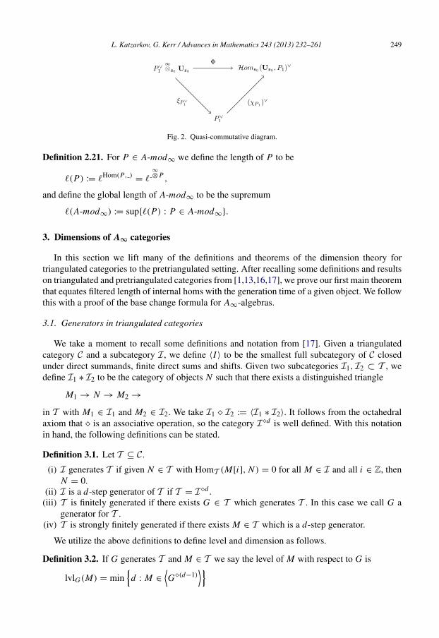
complex as P2 = Ds0 we restrict ξ to obtain the quasi-commutative diagram in Fig. 2.

By exactness of P∨

1

∞

⊗s0 and Homs0( , P1)∨ and naturality of Ψ , we have that Ψ induces

a quasi-isomorphism on perfect s2 polymodules. As was observed above, Ψ respects filtrationswhich yields the claim. �

As a corollary, we have the following important fact

Corollary 2.20. Suppose A ∈ Alg∞ and P ∈ A-mod∞. Then

ℓHom(P, )= ℓ

∞

⊗ P .

This equality motivates the following definition.


Fig. 2. Quasi-commutative diagram.

Definition 2.21. For P ∈ A-mod∞ we define the length of P to be

ℓ(P) := ℓHom(P, )= ℓ

∞

⊗ P ,

and define the global length of A-mod∞ to be the supremum

ℓ(A-mod∞) := sup{ℓ(P) : P ∈ A-mod∞}.

3. Dimensions of A∞ categories

In this section we lift many of the definitions and theorems of the dimension theory fortriangulated categories to the pretriangulated setting. After recalling some definitions and resultson triangulated and pretriangulated categories from [1,13,16,17], we prove our first main theoremthat equates filtered length of internal homs with the generation time of a given object. We followthis with a proof of the base change formula for A∞-algebras.

3.1. Generators in triangulated categories

We take a moment to recall some definitions and notation from [17]. Given a triangulatedcategory C and a subcategory I , we define ⟨I ⟩ to be the smallest full subcategory of C closedunder direct summands, finite direct sums and shifts. Given two subcategories I1, I2 ⊂ T , wedefine I1 ∗ I2 to be the category of objects N such that there exists a distinguished triangle

M1 → N → M2 →

in T with M1 ∈ I1 and M2 ∈ I2. We take I1 � I2 := ⟨I1 ∗ I2⟩. It follows from the octahedralaxiom that � is an associative operation, so the category I �d is well defined. With this notationin hand, the following definitions can be stated.

Definition 3.1. Let T ⊆ C.

(i) I generates T if given N ∈ T with HomT (M[i], N ) = 0 for all M ∈ I and all i ∈ Z, thenN = 0.

(ii) I is a d-step generator of T if T = I �d .(iii) T is finitely generated if there exists G ∈ T which generates T . In this case we call G a

generator for T .(iv) T is strongly finitely generated if there exists M ∈ T which is a d-step generator.

We utilize the above definitions to define level and dimension as follows.

Definition 3.2. If G generates T and M ∈ T we say the level of M with respect to G is

lvlG(M) = min

d : M ∈

G�(d−1)


Fig. 3. Quivers of generators for Db(P1).

and the generation time of G is

t (G) = min

d : T =

G�(d−1)

= max {lvlG(M) : M ∈ T } .

The dimension of a category T with generators is defined to be the smallest generation time.The Orlov spectrum of T is the set of all generation times.

The central theme of this paper is to enhance the above definitions into the language of DG andA∞-categories. Thus we will assume our category T is always a subcategory of the homotopycategory H0(A) for some pretriangulated A∞-category A. If T is an algebraic triangulatedcategory, this is implied by a theorem of Lefevre-Hasegawa which we site below. Recall thata triangulated category is algebraic if it is the stable category of a k-linear Frobenius category(see [11]). First we fix notation and, in a triangulated category T , write Hom∗

T (M, N ) for thealgebra ⊕n∈Z HomT (M, N [n]).

Theorem 3.3 (7.6.0.4, [13]). If T is an algebraic triangulated category which is stronglygenerated by an object G, then there is an A∞ structure on AG := Hom∗

T (G,G) such thatthe Yoneda functor evaluated at G from T to H0(AG-mod∞) is a triangulated equivalence.

We say that a pretriangulated A∞-subcategory B (strongly) generates if H0(B) does inH0(A). We also use the same language and notation as above for level, generation time anddimension.

Before proceeding with this discussion, we take a moment to illustrate this theorem with someexamples.

Example 3.4. For Pn , Beilinson showed [2] that ⟨O,O(1), . . .O(n)⟩ forms a full exceptionalcollection for Db(Pn). Taking G = ⊕

ni=0 O(i) then gives a generator. From grading considera-

tions, the endomorphism algebra AG has no higher products so Db(Pn) ≃ H0(AG-mod∞). Inthe case of n = 1, AG is the path algebra of the Kronecker quiver illustrated in Fig. 3.

Exceptional collections in the dimension theory of triangulated categories were studied in [1].In general, one can mutate an exceptional collection to obtain a new exceptional collectionand thereby a new generator. Below we examine a generator which does not arise from suchmutations and in fact is not defined as the direct sum of objects in an exceptional collection.

Example 3.5. Let n = 1 in the previous example and let G ′= O ⊕ O p where p ∈ P1 is any

point. The algebra AG ′ is the quiver algebra with relations given in the middle of Fig. 3 wheredeg(a) = 1 = deg(c) and deg(b) = 0 and ba = c. Here, the grading does not preclude theexistence of higher products, but it is not hard to exhibit a quasi-isomorphism from this algebrato the DG algebra endomorphism algebra of the mutated objects in AG-mod∞. Again we obtainthe isomorphism Db(P1) ≃ H0(AG ′ -mod∞) from coherent sheaves to graded modules over thegraded algebra AG ′ .

Example 3.6. Another studied example is the category of matrix factorizations for the functionfn : C → C via fn(z) = zn , or equivalently the derived category of singularities Db

sg( f −1n (0)).


It was observed in [1] that every non-zero object of M F(C[[z]], fn) is a strong generator andthat the generator

C C∈ M F(C[[z]], fn)

zn−1

z

which is equivalent to O0 ∈ Dbsg( f −1

n (0)) had maximal generation time. Also, in [8], the com-putation of a minimal model for AG as a Z/2Z graded A∞-algebra was performed and foundto equal AG = k[θ ]/(θ2) where deg(θ) = 1 and all higher products vanish except µn(θ, θ,

. . . , θ) = 1. Again, we have Dbsg( f −1

n (0)) ≃ H0(AG-mod∞).

Now, starting with an A∞ pretriangulated category A, let G ∈ A be a generator and AG =

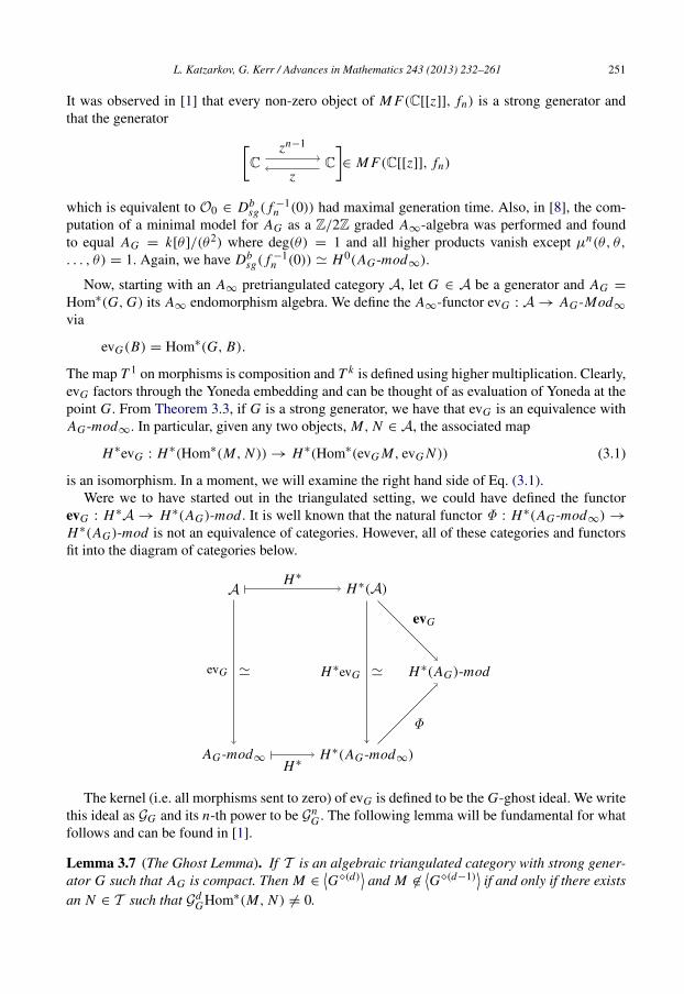
Hom∗(G,G) its A∞ endomorphism algebra. We define the A∞-functor evG : A → AG-Mod∞

via

evG(B) = Hom∗(G, B).

The map T 1 on morphisms is composition and T k is defined using higher multiplication. Clearly,evG factors through the Yoneda embedding and can be thought of as evaluation of Yoneda at thepoint G. From Theorem 3.3, if G is a strong generator, we have that evG is an equivalence withAG-mod∞. In particular, given any two objects, M, N ∈ A, the associated map

H∗evG : H∗(Hom∗(M, N )) → H∗(Hom∗(evG M, evG N )) (3.1)

is an isomorphism. In a moment, we will examine the right hand side of Eq. (3.1).Were we to have started out in the triangulated setting, we could have defined the functor

evG : H∗A → H∗(AG)-mod. It is well known that the natural functor Φ : H∗(AG-mod∞) →

H∗(AG)-mod is not an equivalence of categories. However, all of these categories and functorsfit into the diagram of categories below.

A H∗(A)

AG-mod∞ H∗(AG-mod∞)

H∗(AG)-mod

H∗

H∗

≃evG ≃H∗evG

evG

Φ

The kernel (i.e. all morphisms sent to zero) of evG is defined to be the G-ghost ideal. We writethis ideal as GG and its n-th power to be G n

G . The following lemma will be fundamental for whatfollows and can be found in [1].

Lemma 3.7 (The Ghost Lemma). If T is an algebraic triangulated category with strong gener-ator G such that AG is compact. Then M ∈

G�(d)

and M ∈

G�(d−1)

if and only if there exists

an N ∈ T such that G dGHom∗(M, N ) = 0.


An important conceptual point about this perspective is that, by choosing a generating objectG, the homotopy category of A has been enhanced to a filtered category. This is not an invariantof the A∞-category A, nor is it an invariant of the triangulated category H∗A. It is an additionalstructure introduced by the choice of generator which provides homological information relativeto G.

3.2. Ghosts and length

We will now establish the link between generation time and filtration length. The followinglemma is straightforward, but we supply a proof to establish some notation.

Lemma 3.8. In A-Mod∞ we have ℓ(UA) = 0.

Before we begin the proof, we set up the more general comodule notation and define a weakerclass of maps Mapk

C (P, P ′) between two DG comodules of a coalgebra C . First, given a DGcoalgebra C ∈ Cog and DG comodule P , we have a canonical filtration on P given by

P[k] := ker(∆kP ).

The analogue of the length filtration in (2.11) for DG comodules is then

F i Hom(P, P ′) = {φ : φ(P[k]) ⊆ P[k−i]}.

This induces a filtration F• on the cohomology of Hom(P, P ′). We will often abuse notationand write φ ∈ Fk to indicate that the cohomology class [φ] ∈ Fk . In the context of the DGcategory of A-modules Mod∞ for some A∞ algebra A, it follows from the definition that thelength filtration in (2.11) equals that of the F • filtration on the bar constructions

F •HomMod∞(M, N ) = F •Hom(BM,BN ).

This filtration is on morphisms in the pretriangulated category Mod∞, while the filtration F•

is on morphisms H∗(HomMod∞(M, N )) or H0(HomMod∞

(M, N )) in the derived categoryH∗(Mod∞) or H0(Mod∞) respectively.

For any map of comodules f : P → P ′, we take

[∆, f ] := ∆P ′ f − (1C ⊗ f )∆P

and note that

[∆, f g] = (1C ′ ⊗ f ⊗ 1C )[∆, g] + [∆, f ]g.

For k ≥ 0, define

MapkC (P, P ′) =

f : image([∆, f ]) ⊂ C ⊗ P ′

[k]

.

It is immediate that the vector spaces Map•

C (P, P ′) form an increasing filtration. These classesof maps will be useful when defining homotopies. Indeed, they naturally appear in the cobarcomplex of morphisms from the cobar of P to the cobar of P ′ satisfying filtration properties ontheir differential in that complex. A straightforward generalization Mapk,l

C0,C1(P, P ′) of the above

definition to (C0,C1) bicomodules P and P ′ will also be used. We leave the elementary proof ofthe following properties to the reader.


Lemma 3.9. (i) If f ∈ MapkC (P, P ′), g ∈ F i Hom(P ′, P ′′) with k ≤ i , then g f ∈ F i−k

Hom(P, P ′′).(ii) If f ∈ Mapk

C (P, P ′) then f (P[n]) ⊆ P ′

[n+k].

(iii) If f ∈ MapkC (P, P ′), g ∈ Mapi

C (P′, P ′′) then g f ∈ Mapk+i

C (P, P ′′).(iv) If f ∈ Mapk

C (P, P ′) then ∂ f ∈ MapkC (P, P ′).

Utilizing these properties, we proceed with the proof of Lemma 3.8.

Proof (Proof of Lemma 3.8). To prove the lemma, we define a homotopy contraction

h A : BUA → BUA

as

∞

m=1 1⊗m⊗ η where η is the insertion of the identity. More concretely,

h A([a1| · · · |am]) = (−1)|a1|+···+|am |[a1| · · · |am |e]

where |ai | is the degree of ai in A[1]. A quick computation shows that indeed

h AbA + bAh A = 1

so that h A is a vector space contracting homotopy of BUA.Note that h A is not a B A-comodule morphism of BUA (otherwise, the entire category

A-Mod∞ would be zero). Indeed, we have, for any a ∈ BUA,

(∆h A − (1 ⊗ h A)∆)(a) = (−1)|a|a ⊗ [e]

This implies that h A ∈ Map1B A(BUA,BUA). By Lemma 3.9, we have that if φ ∈ F 1

HomMod∞(UA,M) then bφ ◦ h A ∈ Map0

B A(BUA,BUA) is a comodule morphism. Thus, ifφ ∈ F 1HomMod∞

(A,M) is a homomorphism, then ∂(bφh A) = bφ∂h A = bφ implying thatit is a boundary and therefore F1Hom(UA,M) = 0. �

Applying this lemma yields the following corollary.

Corollary 3.10. For any A∞-algebra A, G A = F1.

Proof. Clearly, if φ : M → N is in F 1, then φ∗ : HomMod∞(A,M) → F 1Hom(A, N ) so

[φ]∗ = 0. Conversely, using the homotopy retract above, one sees that there exists a map

HomMod∞(A, K ) → HomMod∞

(A, K )/F 1HomMod∞(A, K )

which is natural with respect to K ∈ Mod∞. This induces a natural inclusion

Hom(A, K ) ↩→ Hommod(H(A), H(K )),

≃ H(K ).

Thus if [φ]∗ = 0 then [φ0] = 0 implying [φ] ∈ F1Hom(M, N ). �

Indebted to the compatibility of the length filtration with composition, we also easily obtain.

Corollary 3.11. For all r we have GrA ⊆ Fr .

The following theorem asserts that this inclusion is an equality.

Theorem 3.12. For any A∞-algebra A, GrA = Fr .


Proof. We start this proof by writing down two homotopies of the diagonal (A, A)-bimodule

h±

diag : BA → BA

where

h+

diag([a|a|a′]) = (−1)|a|+|a|

[[a|a]|e|a′]

h−

diag([a|a|a′]) = (−1)|a|

[a|e|[a|a′]].

While these maps fail to be bicomodule morphisms, it is the case that h+

diag ∈ Map1,0B A,B A

(DA,DA) and h−

diag ∈ Map0,1B A,B A(DA,DA). Indeed, we have

[∆, h+

diag]([a|a|a′]) = [a|a] ⊗ [e] ⊗ [a′

]

and

[∆, h−

diag]([a|a|a′]) = [a] ⊗ [e] ⊗ [a|a′

].

Furthermore, letting τ± be the translation maps

τ+(a|a|[a′

1| · · · |a′m]) = (−1)1+|a|+|a|

[[a|a]|a′

1|[a′

2| · · · |a′m]],

τ−([a1| · · · |an]|a|[a′]) = (−1)1+|a1|+···+|an−1|[[a1| · · · |an−1]|an|[a|a′

]],

our homotopies bound to

∂h±

diag = 1 − τ±.

Thus τ− ∈ Map0,1B A,B A(DA,DA) by part (iv) of Lemma 3.9. More generally, we have

∂h±

diag(1 + τ± + τ 2± + · · · + τ k−1

± )

= 1 − τ k±.

We observe that, from the fact that Map0,•(DA,DA) is an increasing filtration, and by part (iii)of Lemma 3.9,

σ−

k := h±

diag(1 + τ± + τ 2± + · · · + τ k−1

± ) ∈ Map0,k(B A,B A)(BDA,BDA). (3.2)

Finally, we note that for any l, as a map in Ch the translation map satisfies

τ k−(B(k,l)DA) = 0. (3.3)

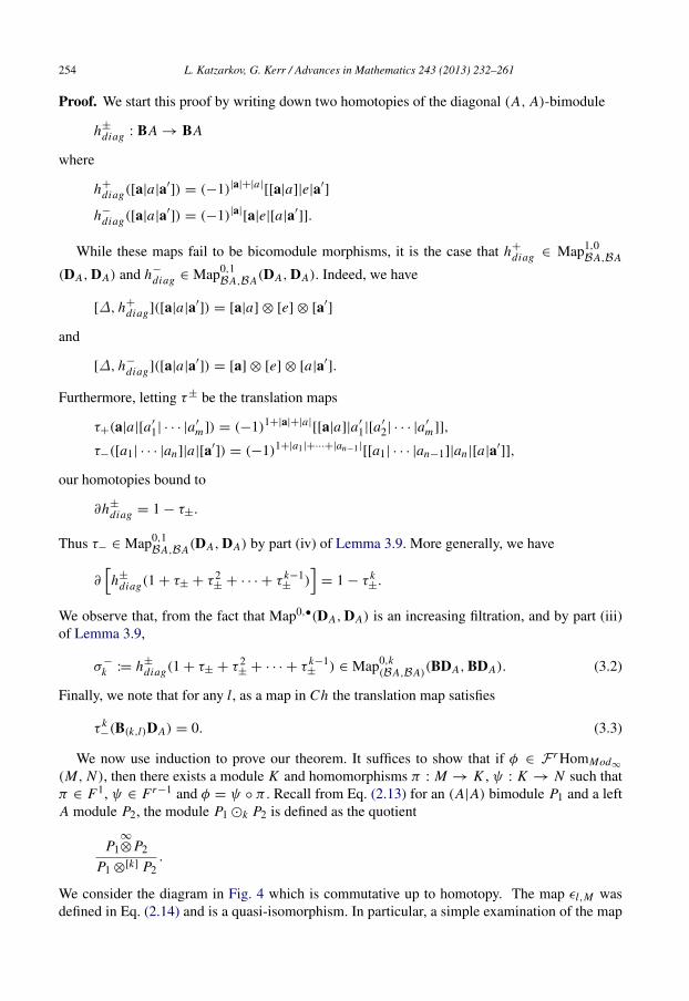
We now use induction to prove our theorem. It suffices to show that if φ ∈ F r HomMod∞

(M, N ), then there exists a module K and homomorphisms π : M → K , ψ : K → N such thatπ ∈ F1, ψ ∈ Fr−1 and φ = ψ ◦ π . Recall from Eq. (2.13) for an (A|A) bimodule P1 and a leftA module P2, the module P1 ⊙k P2 is defined as the quotient

P1∞

⊗P2

P1 ⊗[k] P2.

We consider the diagram in Fig. 4 which is commutative up to homotopy. The map ϵl,M wasdefined in Eq. (2.14) and is a quasi-isomorphism. In particular, a simple examination of the map


Fig. 4. Diagram factoring φ.

shows thatDA

∞

⊗M,

DA ⊗[n−1] M

n∈Z

has length 0 as a filtered module. We note that the proof of Lemma 3.19 is independent of the

results of this section and apply it here. Taking p = 0, N = DA∞

⊗M , Nt = DA ⊗[t] M and

n = 0, Lemma 3.19 implies that π ∈ F1.On the other hand, as ψ is the restriction of ξl,M ◦ (1 ⊗ φ), we can write it out concretely. It

is a strict map whose restriction to A ⊗ A[1]⊗n

⊗ M is

ψ0n ([a|a1| · · · |an|m]) =

ni=0

(−1)|a1|+···+|ai |µi+1N ([a|a1| · · · |ai |φ

n−i ([ai | · · · |an|m])])

for n > 1. As φ ∈ Fr , we see in particular that ψ0n = 0 for n ≤ r . Thus ψ factors as a

composition

A ⊙1 Mπ

−→ A ⊙r Mψ

−→ N

where ψ is a strict homomorphism. Utilizing equation (3.2), a direct calculation shows thatσr−1 ⊗ 1M : BDA ⊗K BM → BDA ⊗K BM restricts to a well defined A∞-module morphism

σ−

r−1 ⊙1 1M : A ⊙1 M → A ⊙r M.

Composing with ψ and applying the differential gives

∂[(−1)|ψ |ψ ◦ (σ−

r−1 ⊙1 1M )] = ψ ◦ ((∂σ−

r−1)⊙1 1M )

= ψ ◦ ((1A − τ r−1− )⊙1 1M )

= ψ ◦ (1A ⊙1 1M )− ψ ◦ (τ r−1− ⊙1 1M )

= ψ ◦ π − ψ ◦ (τ r−1− ⊙1 1M )

= ψ − ψ ◦ (τ r−1− ⊙1 1M ).

Thus ψ is cohomologous to ψ ◦ (τ r−1− ⊙1 1M ). Yet, by Eq. (3.3) we have that

(τ r−1− ⊙1 1M )

B(r−1,0)DA ⊗K BM

= 0

and since ψ is strict, this implies that

ψ ◦ (τ r−1− ⊙1 1M )

B(r−1,0)DA ⊗K BM

= 0.

Thus, ψ ≃ ψ ◦ (τ r− ⊙1 1M ) ∈ Fr−1. �


Combining this theorem with the Ghost Lemma of the previous section, we have the followinghomological criteria for generation time.

Corollary 3.13. Given an A∞-algebra A, the generation time of an A∞-module UA inH0(A-Mod∞) is the global length ℓ(A-mod∞).

Coupling this to the theory of enhanced triangulated categories, we also obtain the corollarybelow.

Corollary 3.14. If A is a pretriangulated A∞-category and G ∈ A is a generator, thent (G) = ℓ(AG-Mod∞).

More refined statements on the level lvlG(M) of an object with respect to a given generatorG are also of use. We write the result in the A∞-module category as opposed to concentratingon the AG-module case.

Corollary 3.15. If M is an A-module then lvlA(M) = ℓ(M).

Example 3.16. As was mentioned at the end of Section 2.1, when AG is an ordinary algebra,the global length of ℓ(AG-Mod∞) is precisely its homological dimension. For the cases ofthe Beilinson exceptional collection ⟨O, . . . ,O(n)⟩, one may use Beilinson’s resolution of thediagonal to see that this dimension is n.

Example 3.17. For the generator O ⊕ O p of P1, we again have formality, but AG ′ is now agraded algebra. Viewing G ′ as a quiver with relations whose vertices correspond to O and O p,one observes that the graded simple modules S1 and S2 arise from considering the idempotentsat the vertices while the graded projective modules P1, P2 from considering all arrows mappingout of each vertex. The projective resolutions below for the simple objects give the homologicaldimension of AG ′ as 2.

· · · 0 → P1 → P2 → P1 → S1 → 0

· · · 0 → P1 → P2 → S2 → 0.

The final example explores a case where higher products have a significant effect on genera-tion time.

Example 3.18. From Example 3.6, we recalled that M F(C[[z]], zn) had a generator G withAG = k[θ ]/(θ2) with a single higher product µn(θ, . . . θ) = 1. To describe H0(AG-mod∞),we examine the A∞-relation for the products of a minimal AG-module M . First, we recall thatM is Z/2Z graded and the usual A∞-module map µr

M : ArG ⊗ M → M is degree r + 1 (due

to the desuspension of AG). Since we assume M is unital, µrM is completely determined by

µrM ([θ | · · · |θ |m]). Writing Lr = µr

M ([θ | · · · |θ | ]) ∈ Hom1gr (M,M), we may condense µM

into a power series L =

∞

r=1 Lr ur∈ Hom1

gr (M,M) ⊗ C[[u]]. It is not hard to see that theA∞-relation on µr

M translates into the equality

L · L = 1M · un .

Decomposing M into its graded summands M = M0 ⊕ M1, we may split Lr = L0r ⊕ L1

r whereL0

r : M0 → M1 and L1r : M1 → M0. Summing, we write Li

=

∞

r=1 L ir ur and after tensoring


M with C[[u]] we then have

M0 ⊗ C[[u]] M1 ⊗ C[[u]]

L0

L1

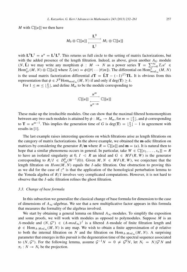
with L0L1= un

= L1L0. This returns us full circle to the setting of matrix factorizations, butwith the added presence of the length filtration. Indeed, as above, given another AG module(N , L) we may write any morphism φ : M → N as a power series T =

∞

r=0 Tr ur∈

Hom∗gr (M, N )⊗ C[[u]] where Tr (m) = φ([θ | · · · |θ |m]). The differential on Hom∗

mod∞(M, N )

is the usual matrix factorization differential dT = LT − (−1)|T |TL. It is obvious from thisrepresentation that φ ∈ F kHommod∞

(M, N ) if and only if deg(T) ≥ k.For 1 ≤ m ≤ ⌊

n2 ⌋, and define Mm to be the module corresponding to

C[[u]] C[[u]]

um

un−m

These make up the irreducible modules. One can show that the maximal filtered homomorphismbetween any two such modules is attained by φ : Mm → Mm , for m = ⌊

n2 ⌋, and φ corresponding

to T = um−1. This implies the generation time of G is deg(T) = ⌊n2 ⌋ − 1 in agreement with

results in [1].

The last example raises interesting questions on which filtrations arise as length filtrations onthe category of matrix factorizations. In the above example, we obtained the m-adic filtration onmatrices by considering the generator R/m where R = C[[u]] and m = (u). It is natural then tohope that a similar phenomena occurs in general. In particular, take W ∈ C[[x1, . . . , xn]] = Rto have an isolated singularity at 0, I ▹ R an ideal and G ∈ M F(R,W ) is the generatorcorresponding to R/I ∈ Db

sg(W−1(0)). Given M, N ∈ M F(R,W ), we conjecture that the

length filtration on Hom(M, N ) equals the I -adic filtration. One obstruction to proving thisas we did for the case of zn is that the application of the homological perturbation lemma tothe Yoneda algebra of R/I involves very complicated computations. However, it is not hard toobserve that the I -adic filtration refines the ghost filtration.

3.3. Change of base formula

In this subsection we generalize the classical change of base formula for dimension to the caseof dimensions of A∞-algebras. We see that a new multiplicative factor appears in this formulathat measures the formality of the algebras involved.

We start by obtaining a general lemma on filtered A∞-modules. To simplify the expositionand some proofs, we will work with modules as opposed to polymodules. Suppose M is anA-module and (N ,G∗) ∈ (A-mod∞)

f is a filtered A-module of finite filtration length andφ ∈ HomA-Mod∞

(M, N ) is any map. We wish to obtain a finite approximation of φ relativeto both the internal filtration on N and the filtration on HomA-Mod∞

(M, N ). A surprisingparameter that emerges in this pursuit is the degeneration time of the spectral sequence associatedto (N ,G∗). For the following lemma, assume G−1 N = 0 = G 0 N , let Nt = N/G t N andπt : N → Nt be the projection.


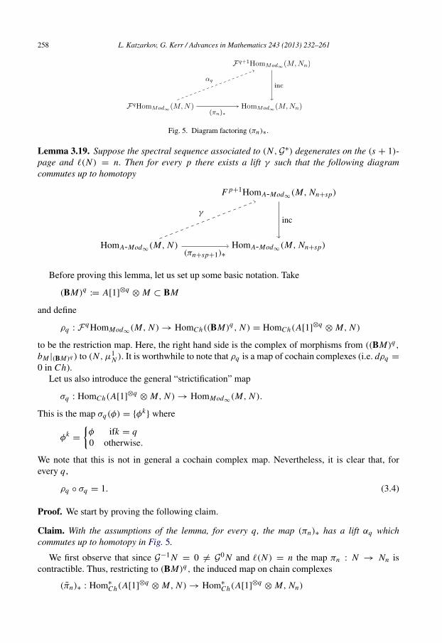
Fig. 5. Diagram factoring (πn)∗.

Lemma 3.19. Suppose the spectral sequence associated to (N ,G∗) degenerates on the (s + 1)-page and ℓ(N ) = n. Then for every p there exists a lift γ such that the following diagramcommutes up to homotopy

HomA-Mod∞(M, N ) HomA-Mod∞

(M, Nn+sp)

F p+1HomA-Mod∞(M, Nn+sp)

(πn+sp+1)∗

γinc

Before proving this lemma, let us set up some basic notation. Take

(BM)q := A[1]⊗q

⊗ M ⊂ BM

and define

ρq : F qHomMod∞(M, N ) → HomCh((BM)q , N ) = HomCh(A[1]

⊗q⊗ M, N )

to be the restriction map. Here, the right hand side is the complex of morphisms from ((BM)q ,bM |(BM)q ) to (N , µ1

N ). It is worthwhile to note that ρq is a map of cochain complexes (i.e. dρq =

0 in Ch).Let us also introduce the general “strictification” map

σq : HomCh(A[1]⊗q

⊗ M, N ) → HomMod∞(M, N ).

This is the map σq(φ) = {φk} where

φk=

φ ifk = q0 otherwise.

We note that this is not in general a cochain complex map. Nevertheless, it is clear that, forevery q,

ρq ◦ σq = 1. (3.4)

Proof. We start by proving the following claim.

Claim. With the assumptions of the lemma, for every q, the map (πn)∗ has a lift αq whichcommutes up to homotopy in Fig. 5.

We first observe that since G−1 N = 0 = G 0 N and ℓ(N ) = n the map πn : N → Nn iscontractible. Thus, restricting to (BM)q , the induced map on chain complexes

(πn)∗ : Hom∗

Ch(A[1]⊗q

⊗ M, N ) → Hom∗

Ch(A[1]⊗q

⊗ M, Nn)


is also contractible. Here the differential associated to A[1]⊗q

⊗ M is the restriction of bM . Weuse the notation of πn above in order to distinguish it from the map in the claim, but both areobtained through composition and the equation

ρq ◦ (πn)∗ = (πn)∗ ◦ ρq (3.5)

holds. Let

τ : Hom∗

Ch(A[1]⊗q

⊗ M, N ) → Hom∗−1Ch (A[1]

⊗q⊗ M, Nn)

be a cochain bounding (πn)∗ (i.e. (πn)∗ = dτ in Ch) and take

αq(φ) = [(πn)∗ − d(σq ◦ τ ◦ ρq)](φ).

Observe that, for every φ, this is a cocycle by virtue of (πn)∗ being a cochain map and thefact that d f is a cochain map for any f in Ch. It is equally obvious that the diagram in Fig. 5then commutes up to homotopy. So the only point left to prove for the claim is that any modulehomomorphism φ ∈ HomMod∞

(M, N ) has image in F q+1HomMod∞(M, Nn). This is true iff

ρq(αq(φ)) = 0. Since ρq is a chain map, we have ρq(dg) = d(ρq(g)), and by Eqs. (3.4), (3.5)

ρq(αq(φ)) = ρq([(πn)∗ − d(σq ◦ τ ◦ ρq)](φ))

= ρq ◦ (πn)∗(φ)− ρq [d(σq ◦ τ ◦ ρq)(φ)]

= (πn)∗ ◦ ρq(φ)− d[(ρq ◦ σq ◦ τ ◦ ρq)(φ)]

= (πn)∗ ◦ ρq(φ)− d[(τ ◦ ρq)(φ)]

= (πn)∗ ◦ ρq(φ)− (dτ) ◦ ρq(φ)

= (πn)∗ ◦ ρq(φ)− (πn)∗ ◦ ρq(φ)

= 0.

One now uses the claim to prove the lemma by observing that if (C∗,G) is any filtered chaincomplex whose length is r and whose spectral sequence converges at the (p + 1)-th page, thenℓ(C/Gr C,G) ≤ p. This argument relies on simply unravelling the definition of the spectralsequence associated to a filtration. We recall that the page Eq

k = Zqk /Bq

k is the subquotient ofG kC/G k−1C where

Zqk = {[c] : c ∈ G kC, dc ∈ G k−qC}

and

Bqk = {[dc] : c ∈ G k+q−1C, dc ∈ G kC}.

Note then that Er+qk is the same as Eq

k for q > p where the later is the spectral sequence for(C/Gr C,G∗−r ). In particular, Eq

k = 0 for all q > p implying the length ℓ(C/Gr C,G) ≤ p. Tofinish the proof, just inductively apply the claim above and this observation with (N ,G∗). �

The following theorem is a result of 3.19.

Theorem 3.20. Let P be a (B, A)-bimodule and M a left A-module. Suppose the spectral

sequence of P∞

⊗A M degenerates at the (s+1)-st page. If the convolution functor P∞

⊗ is faithful,then

lvlA(M) ≤ lvlA(P)+ s · lvlB(P∞

⊗A M)


Proof. Assume that this is not the case. Then there exists a nonzero morphism f ∈ Fr Hom∗

(M, N ) with r > lvlA P∨+ s · lvlB(P

∞

⊗A M). Then by definition, 1P∞

⊗ f is zero on P ⊗[r−1] M

implying 1P∞

⊗ f = ψ ◦ πr = π∗r (ψ) where

πr : P∞

⊗M → P ⊙r M.

Now, by assumption, the spectral sequence associated to P∞

⊗A M degenerates at (s + 1) and by2.20,

ℓ(P∞

⊗A M) ≤ ℓ(P∨) = lvlA(P).

Letting n = lvlA P , the following lifting problem is solvable for all p by Lemma 3.19.

HomMod∞(P

∞

⊗ M, P∞

⊗ M) HomMod∞(P

∞

⊗ M, P ⊙n+sp+1 M)

F p+1HomMod∞(P

∞

⊗ M, P ⊙n+sp+1 M)

(πn+sp+1)∗

γinc

In particular, if p = lvlB(P∞

⊗A M) we have that πn+sp+1 ≃ 0. This implies that for all

t ≥ n + sp + 1 = lvlA P∨+ s · lvlB(P

∞

⊗A M)

we must have πt ≃ 0 so that πr ≃ 0 and therefore 1P∞

⊗ f ≃ 0. This contradicts the assumption

that P∞

⊗ is faithful. �

We observe that in the case of formal algebras with formal modules, this theorem reproducesthe classical change of base theorem in the dimension theory of rings. In more generality, it ispossible to relate the constant s with matric Massey products of the algebra A and module M .This quantifies a lack of formality and ties it directly to the Orlov spectrum of a category.

Acknowledgments

Support was provided by NSF Grant DMS0600800, NSF FRG Grant DMS-0652633, FWFGrant P20778, and an ERC Grant — GEMIS. Both authors would like to thank Matt Ballard,Colin Diemer, David Favero, Maxim Kontsevich, Dima Orlov, Pranav Pandit, Tony Pantev andPaul Seidel for helpful comments and conversation during the preparation of this work. Thesecond author would like to thank David Favero in particular for his patient explanations ofresults on the dimension theory of triangulated categories.

References

[1] M. Ballard, D. Favero, L. Katzarkov, Orlov spectra: bounds and gaps. 2011.[2] A. Beilinson, Coherent sheaves on Pn and problems in linear algebra, Funksional. Anal. i Prilozhen. 12 (3) (1978)

68–69.[3] A. Bondal, M. Van den Bergh, Generators and representability of functors in commutative and noncommutative

geometry, Mosc. Math. J. 3 (1) (2003) 1–36.[4] A. Bondal, M. Kapranov, Enhanced triangulated categories, Mat. Sb. 181 (5) (1990) 669–683.


[5] E. Brown, Twisted tensor products. i, Ann. of Math. 69 (2) (1959) 223–246.[6] P. Deligne, D. Freed, Sign manifesto, in: Quantum Fields and Strings: A Course for Mathematicians, vols. 1, 2,

Amer. Math. Soc, 1999, pp. 357–363.[7] V. Drinfeld, DG quotients of DG categories, J. Algebra 272 (2) (2004) 643–691.[8] T. Dyckerhoff, Compact generators in categories of matrix factorizations, Duke Math. J. 159 (2) (2011) 223–274.[9] S. Eilenberg, J. Moore, Homology and fibrations. I. Coalgebras, cotensor product and its derived functors,

Comment. Math. Helv. 40 (1966) 199–236.[10] B. Keller, A∞ algebras, modules and functor categories, in: Proceedings of the workshop of the ICRA XI (Quertaro,

Mexico, 2004), 2005.[11] B. Keller, On differential graded categories, in: Proc. ICM, Madrid, vol. 2, 2006, pp. 151–190.[12] G. Kelly, Basic concepts of enriched category theory, in: London Mathematical Society Lecture Note Series,

vol. 64, Cambridge University Press, 1982.[13] K. Lefevre-Hasegawa, Sur les A∞-categories, Ph.D. Thesis, Universite Denis Diderot Paris 7, November 2003.[14] J. Loday, The diagonal of the Stasheff polytope, in: Higher Structures in Geometry and Physics, in: Progress in

Mathematics, vol. 287, 2011, pp. 269–292.[15] J. Lurie, Higher Topos Theory, in: Annals of Mathematics Studies, vol. 170, Princeton University Press, 2009.[16] D. Orlov, Remarks on generators and dimensions of triangulated categories, Mosc. Math. J. 9 (1) (2009) 143–149.[17] R. Rouquier, Dimensions of triangulated categories, J. K-Theory 1 (2) (2008) 193–256.

orlov spectra as a filtered cohomology theory · the orlov spectrum compares the generation times...

Documents