orthogonal basis and gram schmidth process
TRANSCRIPT

.TOPIC- ORTHOGONAL SET & BASIS THE GRAM-SCHMIDT
PREPARED BY RAJESH GOSWAMI
Outline
Orthogonal Sets Orthogonal basis The Gram-Schmidt Orthogonalization Process
Slide 6.2- 3 © 2012 Pearson Education, Inc.
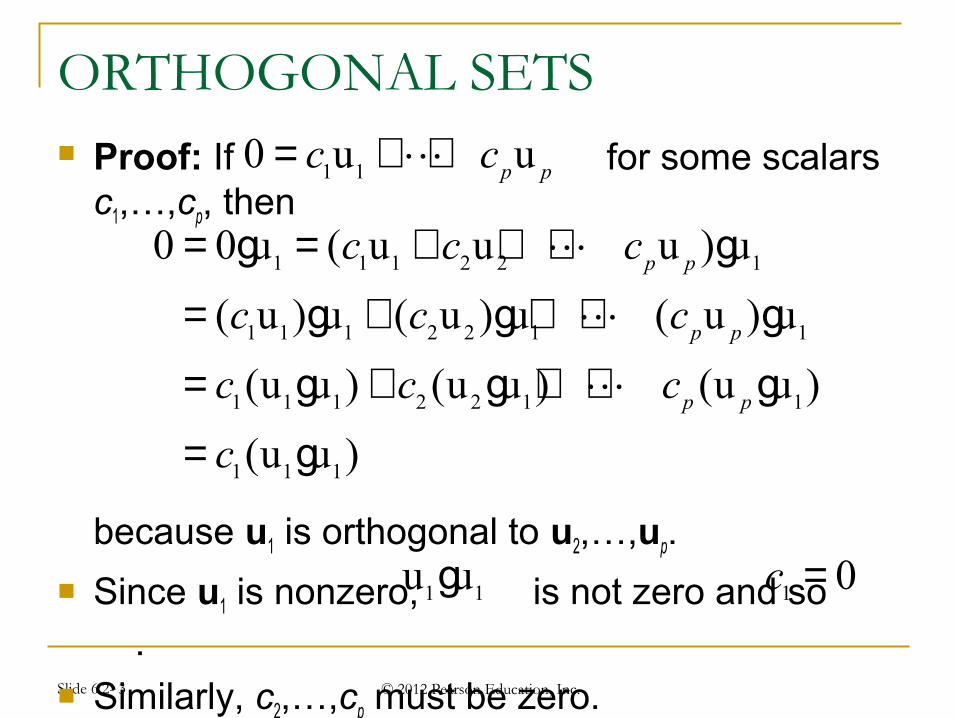
ORTHOGONAL SETS Proof: If for some scalars c1,…,cp, then
because u1 is orthogonal to u2,…,up.
Since u1 is nonzero, is not zero and so .
Similarly, c2,…,cp must be zero.
1 10 u up pc c= + +L
1 1 1 2 2 1
1 1 1 2 2 1 1
1 1 1 2 2 1 1
1 1 1
0 0 u ( u u u ) u
( u ) u ( u ) u ( u ) u
(u u ) (u u ) (u u )
(u u )
p p
p p
p p
c c c
c c c
c c c
c
= = + + +
= + + +
= + + +
=
Lg gLg g gLg g g
g
1 1u ug 1 0c =
Slide 6.2- 4 © 2012 Pearson Education, Inc.
ORTHOGONAL SETS
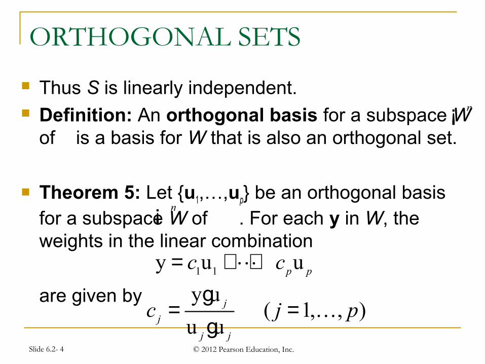
Thus S is linearly independent. Definition: An orthogonal basis for a subspace W
of is a basis for W that is also an orthogonal set.
Theorem 5: Let {u1,…,up} be an orthogonal basis for a subspace W of . For each y in W, the weights in the linear combination
are given by
n¡
n¡
1 1y u up pc c= + +L
y u
u uj
j
j j
c =gg
( 1, , )j p= K
Slide 6.2- 5 © 2012 Pearson Education, Inc.
ORTHOGONAL SETS
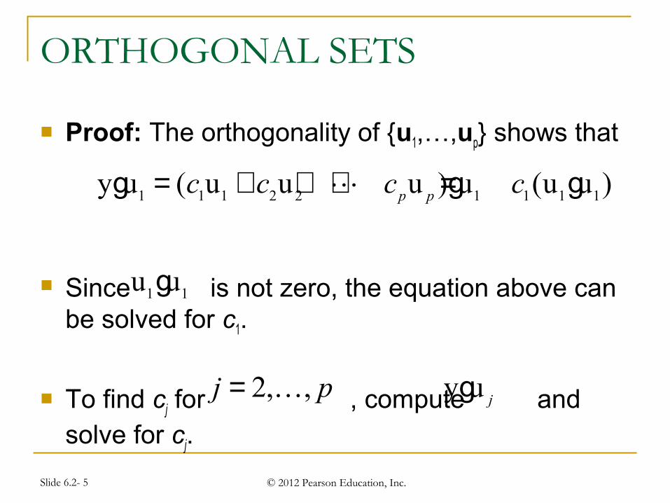
Proof: The orthogonality of {u1,…,up} shows that
Since is not zero, the equation above can be solved for c1.
To find cj for , compute and solve for cj.
1 1 1 2 2 1 1 1 1y u ( u u u ) u (u u )p pc c c c= + + + =Lg g g
1 1u ug
2, ,j p= K y u jg

.
Orthogonal basis: A basis consisting of orthogonal vectors in an inner product space.
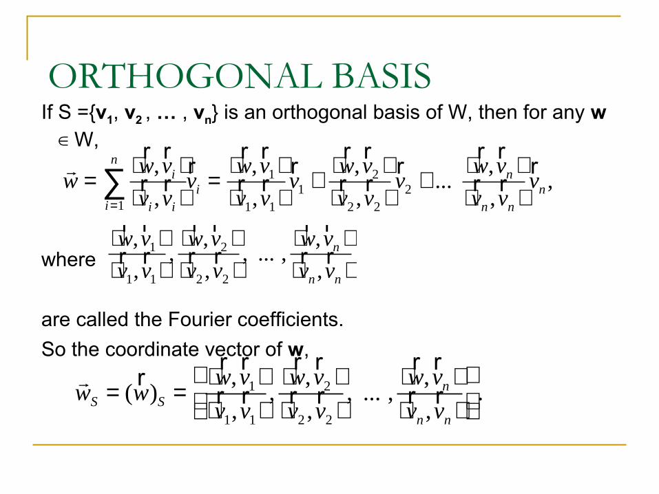
ORTHOGONAL BASIS If S ={v1, v2 , … , vn} is an orthogonal basis of W, then for any w ∈ W,
where
are called the Fourier coefficients.
So the coordinate vector of w,
rw =
⟨ rw,
rvi ⟩
⟨rvi ,
rvi ⟩i=1
n
∑ rvi =
⟨ rw,
rv1⟩
⟨rv1,
rv1⟩
rv1 +
⟨ rw,
rv2 ⟩
⟨rv2 ,rv2 ⟩
rv2 + ...
⟨ rw,
rvn ⟩
⟨rvn ,
rvn ⟩
rvn ,
rwS = (
rw)S =
⟨ rw,
rv1⟩
⟨rv1,
rv1⟩
,⟨ rw,
rv2 ⟩
⟨rv2 ,
rv2 ⟩
, ... ,⟨ rw,
rvn ⟩
⟨rvn ,
rvn ⟩
.
⟨ rw,
rv1⟩
⟨rv1,rv1⟩
,⟨ rw,
rv2 ⟩
⟨rv2 ,rv2 ⟩
, ... ,⟨ rw,
rvn ⟩
⟨rvn ,
rvn ⟩
8
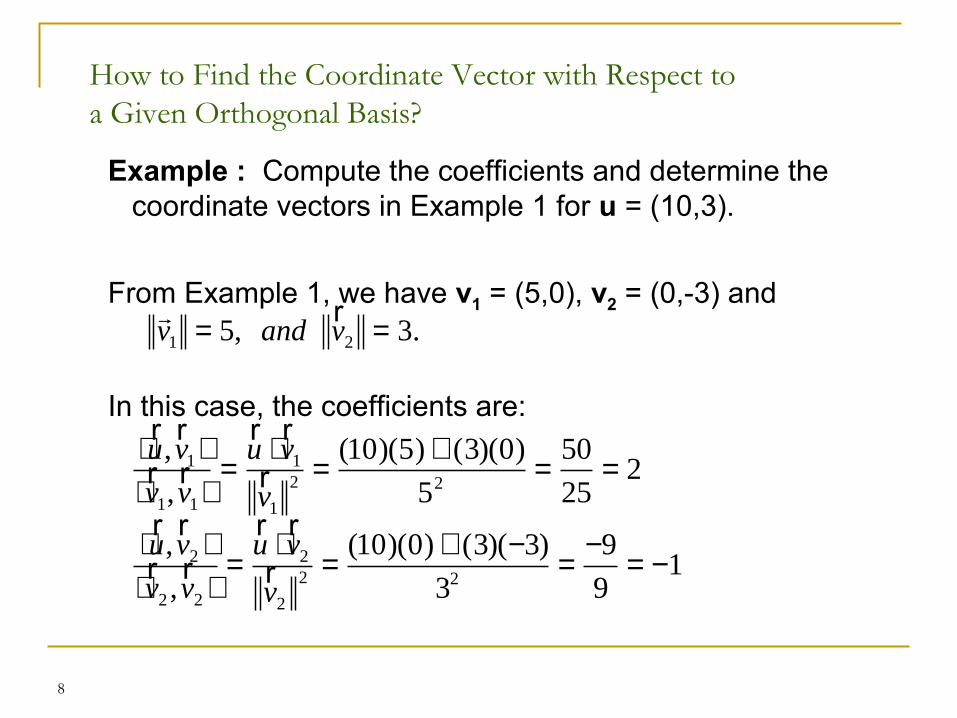
How to Find the Coordinate Vector with Respect to a Given Orthogonal Basis?
Example : Compute the coefficients and determine the coordinate vectors in Example 1 for u = (10,3).
From Example 1, we have v1 = (5,0), v2 = (0,-3) and
In this case, the coefficients are:
⟨ ru,
rv1⟩
⟨rv1,
rv1⟩
=ru ⋅ r
v1rv1
2 =(10)(5) + (3)(0)
52=
50
25= 2
⟨ ru,
rv2 ⟩
⟨rv2 ,
rv2 ⟩
=ru ⋅ r
v2rv2
2 =(10)(0) + (3)(−3)
32=
−9
9= −1
rv1 = 5, and
rv2 = 3.
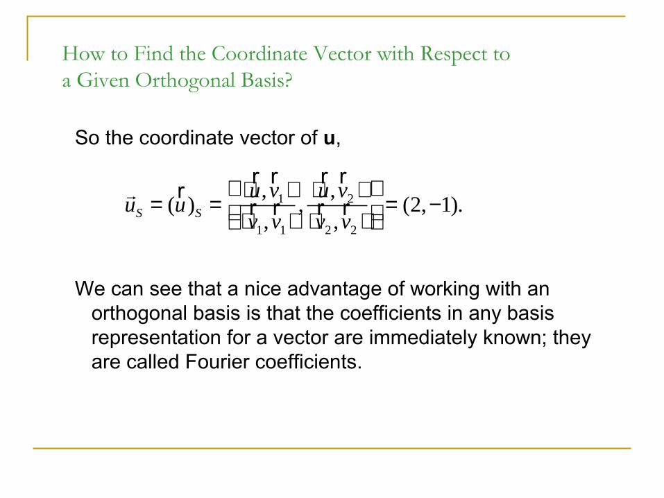
How to Find the Coordinate Vector with Respect to a Given Orthogonal Basis?
So the coordinate vector of u,
We can see that a nice advantage of working with an orthogonal basis is that the coefficients in any basis representation for a vector are immediately known; they are called Fourier coefficients.
ruS = (
ru)S =
⟨ ru,
rv1⟩
⟨rv1,rv1⟩
,⟨ ru,
rv2 ⟩
⟨rv2 ,
rv2 ⟩
= (2,−1).
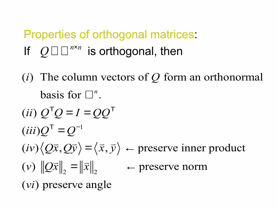
Properties of orthogonal matrices:
If is orthogonal, thenn nQ ×∈ ℜ
1
2 2
( ) The column vectors of form an orthonormal
basis for .
( )
( )
( ) , , preserve inner product
( ) preserve norm
( ) preserve angle
n
i Q
ii Q Q I QQ
iii Q Q
iv Qx Qy x y
v Qx x
vi
Τ Τ
Τ −
ℜ= =
== ←
= ←
Gram-Schmidt Orthogonalization Process
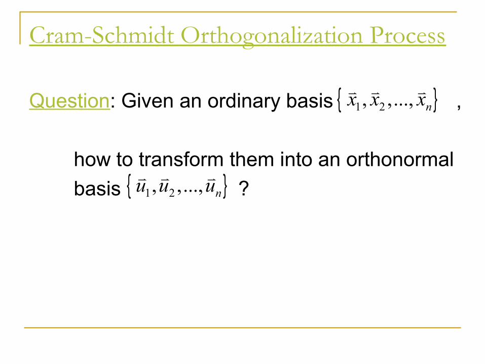
Cram-Schmidt Orthogonalization Process
Question: Given an ordinary basis ,
how to transform them into an orthonormal
basis ?
{ }1 2, ,..., nx x x
{ }1 2, ,..., nu u u
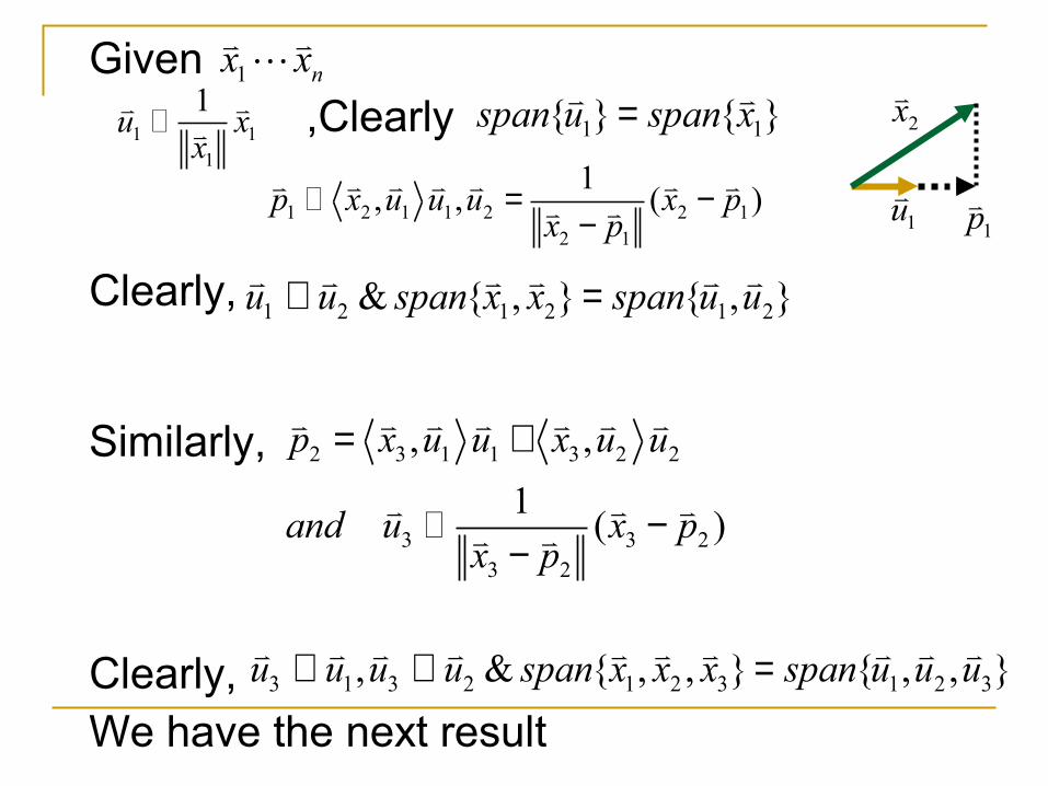
Given ,Clearly
Clearly,
Similarly,
Clearly, We have the next result
1 nx x
1 11
1u x
x 1 1{ } { }span u span x=
1 2 1 1 2 2 12 1
1, , ( )p x u u u x p
x p= −
−
1 2 1 2 1 2& { , } { , }u u span x x span u u⊥ =
2 3 1 1 3 2 2
3 3 23 2
, ,
1( )
p x u u x u u
and u x px p
= +
−−
3 1 3 2 1 2 3 1 2 3, & { , , } { , , }u u u u span x x x span u u u⊥ ⊥ =
1u
1p
2x
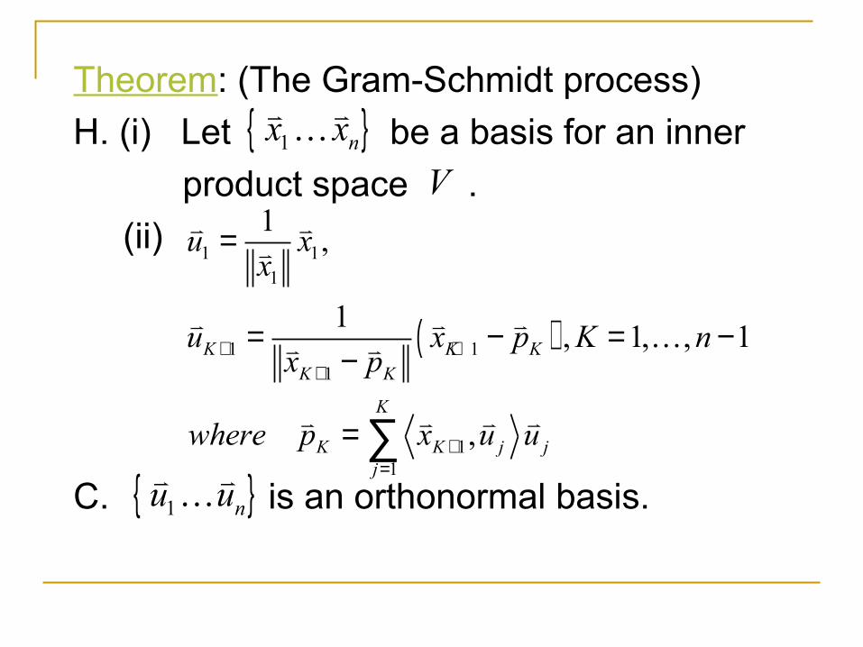
Theorem: (The Gram-Schmidt process)
H. (i) Let be a basis for an inner
product space .
(ii)
C. is an orthonormal basis.{ }1 nu u
{ }1 nx x
V
( )
1 11
1 11
11
1,
1, 1, , 1
,
K K KK K
K
K K j jj
u xx
u x p K nx p
where p x u u
+ ++
+=
=
= − = −−
= ∑
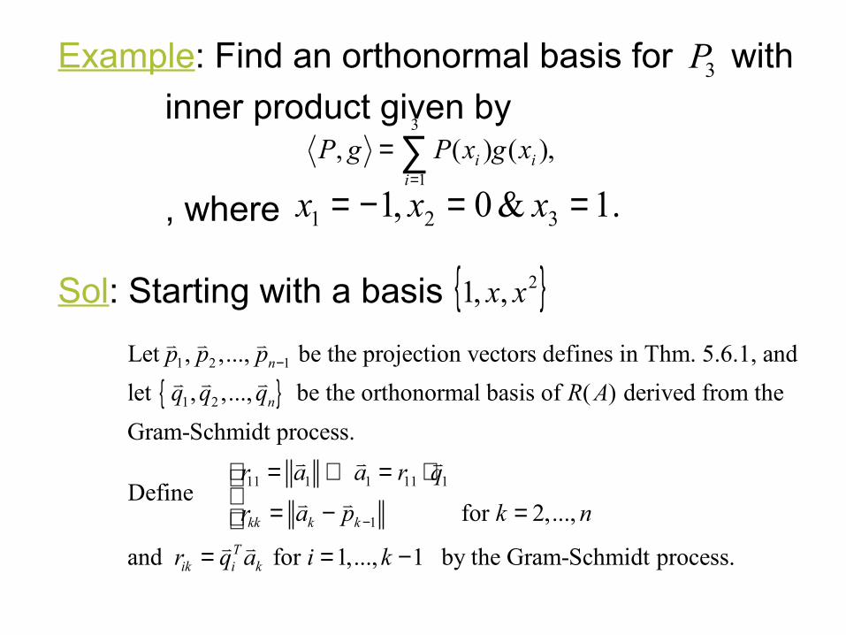
Example: Find an orthonormal basis for with
inner product given by
, where
Sol: Starting with a basis
3P
),()(,3
1i
ii xgxPgP ∑
=
=
.1&0,1 321 ==−= xxx
{ }2,,1 xx
{ }1 2 1
1 2
11 1 1 11 1
Let , ,..., be the projection vectors defines in Thm. 5.6.1, and
let , ,..., be the orthonormal basis of ( ) derived from the
Gram-Schmidt process.
Define
n
n
kk
p p p
q q q R A
r a a r q
r
−
= ⇒ = ⋅
=
1 for 2,...,
and for 1,..., 1 by the Gram-Schmidt process.
k k
Tik i k
a p k n
r q a i k
−
− == = −

Theorem: (QR Factorization)
If A is an m×n matrix of rank n, then A
can be factored into a product QR, where Q
is an m×n matrix with orthonormal columns
and R is an n×n matrix that is upper triangular
and invertible.

Proof. of QR-Factorization
{ }1 2 1
1 2 1
11 1
Let , ,..., be the projection vectors defined in Thm.5.6.1,
and let , ,..., be the orthonormal basis of ( ) derived from
the Gram-Schmidt process.
Define
n
n
kk k k
p p p
q q q R A
r a
r a p
−
−
−
=
−
@ 1
1 11 1
2 12 1 22 2
1 1
and for 1,... -1 for 2,...,
By the Gram-Schmidt process,
Tik i k
n n
r q a i kk n
a r q
a r q r q
a r q
= ==
== +
= +
M M
... nn nr q+
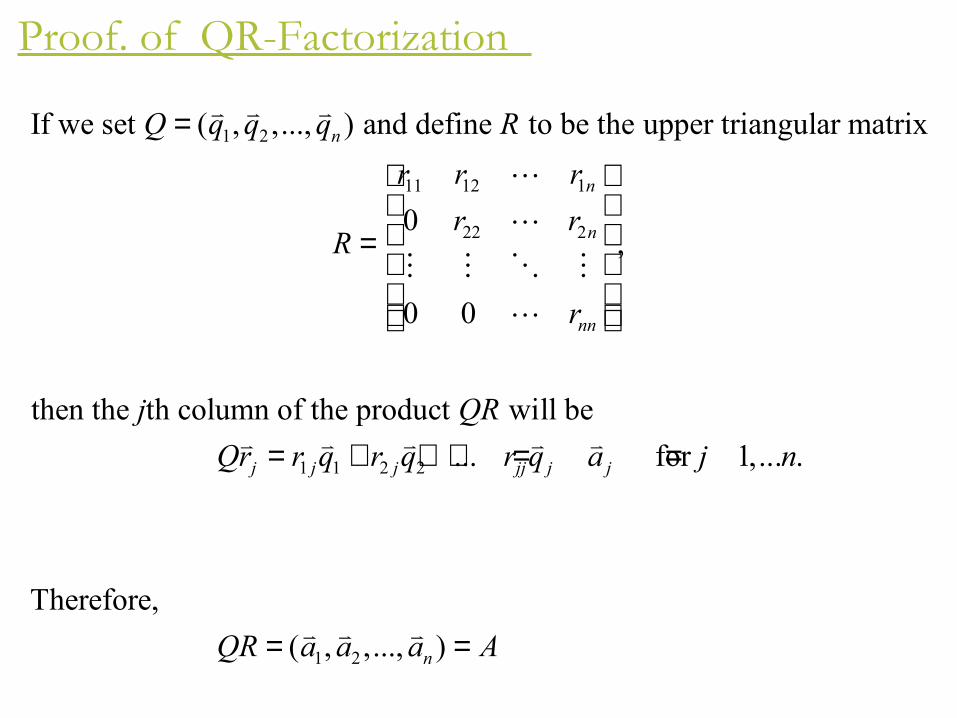
Proof. of QR-Factorization
1 2
11 12 1
22 2
If we set ( , ,..., ) and define to be the upper triangular matrix
0 ,
0 0
then the th column of the product wi
n
n
n
nn
Q q q q R
r r r
r rR
r
j QR
=
=
M M O M
1 1 2 2
1 2
ll be
... for 1,... .
Therefore,
( , ,..., )
j j j jj j j
n
Qr r q r q r q a j n
QR a a a A
= + + + = =
= =

Theorem:
If A is an m×n matrix of rank n, then the
solution to the least squares problem
is given by , where Q and R are the
matrices obtained from Thm.5.6.2. The solution
may be obtained by using back substitution to solve .
Ax b=vv
1x̂ R Q b− Τ=vv
x̂v
ˆRx Q bΤ=vv
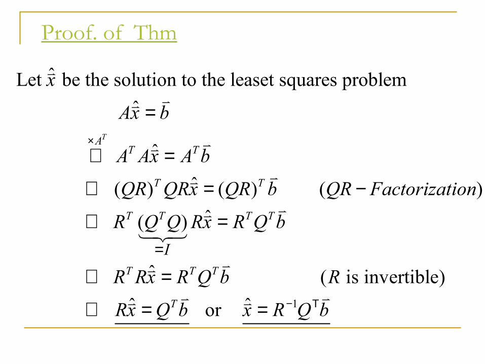
Proof. of Thm
ˆLet be the solution to the leaset squares problem
ˆ
ˆ
ˆ ( ) ( ) ( )
ˆ ( )
TAT T
T T
T T
I
x
Ax b
A Ax A b
QR QRx QR b QR Factorization
R Q Q R
×
=
=
⇒ =
⇒ = −
⇒
v
vv
vv
vv
v
1
ˆ ( is invertible)
ˆ ˆ or
T T
T T T
T
x R Q b
R Rx R Q b R
Rx Q b x R Q b− Τ
=
⇒ =
⇒ = =
v
vv
v vv v

Example : Solve
By direct calculation,
1
2
3
1 2 1 1
2 0 1 1
2 4 2 1
4 0 0 2bA
x
x
x
− − − = − −
v
R
Q
QRA
−
−
−
−
−
−
==200
140
125
1
2
2
4
2
4
1
2
4
2
2
1
5
1
1
1
2
Q bΤ−
= −
v
The solution can be obtained from
5 2 1 1
0 4 1 1
0 0 2 2
⇒− −
− −