Vol. 1, no. 2, 2002

ISSN 1311 - 6797

INTERNATIONAL

MATHEMATICAL JOURNAL

M. Amamiya ( Japan )

J. M. Ash (USA)

T. Colding ( USA)

M. Fliess ( France )

A. Fokas ( UK)

K. Fuller ( USA)

J. Glimm (USA)

W. Goldman ( USA)

F. C. Graham ( USA)

T. Hall (Australia )

M. Hilsum ( France )

D. Hong (USA)

Editorial Board

S. Kichenassamy ( France )

F.- H. Lin (USA)

J. Lyness ( USA)

K. Ono (USA)

I. Prigogine (Belgium)

L. Reichel ( USA)

P. C. Sabatier ( France )

P. Sarnak (USA)

R. Stanley ( USA)

M. Tang ( USA)

W. Veech (USA)

X. Zhou (USA)

Managing Editor: Emil Minchev

International Scientific Publications

International Mathematical Journal

Aims and scopes: The journal will publish carefully selected original

research papers in the area of pure and applied mathematics as follows:

combinatorics, order, lattices, ordered algebraic structures, general

mathematical systems, number theory, field theory and polynomials,

commutative rings and algebras, algebraic geometry, linear and multi linear

algebra, matrix theory, associative and nonassociative rings, category theory,

homological algebra, K- theory, group theory, Lie algebras, real functions,

measure and integration, functions of complex variables, potential theory,

special functions, ordinary differential equations, partial differential

equations, finite difference and functional equations, approximation and

expansion, Fourier analysis, abstract harmonic analysis, integral transforms,

operational calculus, integral equations, functional analysis, operator theory,

calculus of variation and optimal control, optimization, geometry,

differential geometry, topology, manifolds, probability theory and stochastic

processes, statistics, numerical analysis, computer science, mechanics,

thermodynamics, quantum theory, relativity, economics, programming,

games, mathematical biology, information and communication, circuits.

Call for papers: The authors are cordially invited to submit papers in

triplicate to the Managing Editor: Emil Minchev. Manuscripts submitted to

this journal will be considered for publication with the understanding that

the same work has not been published and is not under consideration for

publication elsewhere.

Managing Editor: Dr. Emil Minchev, Department of Mathematics,

Faculty of Education, Chiba University, Yayoi- cho 1-33, lnage- ku,

Chiba 263 - 8522, Japan

e - mail: eminchev@hotmail.com

Intern. Math. Journal, Vol. 1, no. 2, 2002, 133- 147

A REPRESENTATION OF ORTHOGONAL COMPONENTS IN ANALYSIS OF

VARIANCE

Brenton R. Clarke

Mathematics and Statistics, School of Mathematical and Physical Sciences,

Division of Science 8 Engineering, Murdoch University

Murdoch, Westem Australia 6150

ABSTRACT

The history of orthogonal components in the analysis of variance and of the

Helmert transformation is allied to more recent mathematical representations

of Kronecker products. The latter are well known tools useful in the teaching

of factorial designs. Presented here are quick derivations of the usual orthogo­

nal projection matrices associated with independent sums of squares for some

familiar balanced designs. Succinct representations used to form orthogonal

contrasts clearly illustrate the proofs of independence of sums of squares and

give obvious interpretation to degrees of freedom. Resultant central and non­

central chi-squared distributions follow easily. A relationship between recursive

residuals and the Helmert transformation is also noted.

Mathematics Subject Classifications 2000: 62Jl0

Key Words: Helmert transformation; Kronecker Product; Orthogonal pro­

jection matrix; Recursive residuals; Two factor experiment.

134

1. INTRODUCTION

Early in the development of analysis of variance Irwin (1934) gave explicit

expressions for independent squares in the usual randomised block and latin

square experiments in order to explain to students and others interested in

the subject the mathematical theory underlying the "Analysis of Variance"

Method of R.A. Fisher. He alluded to a result of Cochran (1934) where given

x1 , ... , Xn independent normal variables with mean zero and unit standard de­

viation, if xi + ... + x~ = q1 + ... + qk and the q's are each distributed as

chi-squared with degrees of freedom n1 , ... , nk and n = n 1 + ... + nk, then

the q's are all independent. Irwin made use of the Helmert transformation

formulating component sums of squares as the qi which were in turn sums

of squares of independent normal variables. This illustrated independence of

component sums of squares in the analysis of variance. However, Irwin never

used matrix algebra, nor did he refer to the Helmert transformation as such.

Rather, contrasts formulated from coefficients taken from the Helmert matrix

were written out longhand. Helmert transformations are referred to in the

two texts of Searle (1971,1982), though only with respect to the example that

is used in our preliminary illustration in section 2. Other references to the

Helmert transformation are Farebrother (1987) and Lancaster (1965). In this

article Helmert transformations are combined with Kronecker products, also

called direct products in Searle ( 1982), to represent concisely the contrasts

used by Irwin and from there indicate how related simple algebra can be used

to describe higher and more complex experiments with an illustration for the

balanced two factor experiment with replications, allowing for the possibility

of interaction. Properties of Kronecker products given in Rao (1973), Searle

(1982) are thus combined with Helmert matrices to provide concise matrix

representations which lead to orthogonal projection matrices and noncentral

chi-squared distributions. This demonstration which highlights an historical

135

explanation of analysis of variance allied with the more recent advances of Kro­

necker products goes beyond simple discussions of analysis of variance using

the latter products as in Rogers(1984), Saw(1992), and Hocking(1996).

While the Helmert transformation is not necessary in deriving the inde­

pendence of constituent items in the analysis of variance it can be noted that

the original proof of independence of x and s~, the usual sample mean and

variance goes back to Helmert. Fisher (1938) acknowledges Helmert (1875) in

which the chi-squared distribution is first discovered for (n- 1)s~/o-2 • Lan­

caster (1965) makes the first reference to the Helmert transformation as being

due to Helmert (1876) where the independence of x and s~ is discussed. In­

terestingly the contrasts in the analysis of variance for a randomised complete

block design can be described easily using Helmert transformations where co­

incidentally a link is also noted to what are termed the recursive residuals.

2. KRONECKER PRODUCT AND THE HELMERT

TRANSFORMATION

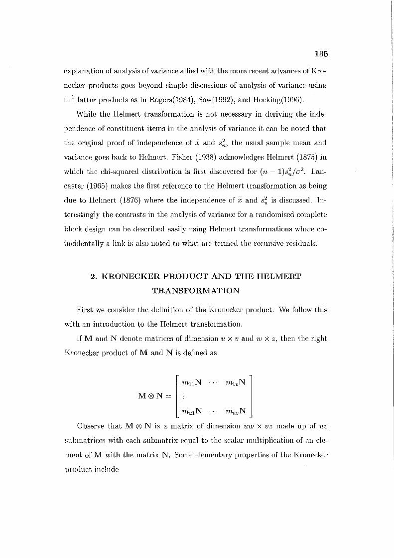
First we consider the definition of the Kronecker product. We follow this

with an introduction to the Helmert transformation.

If M and N denote matrices of dimension u x v and w x z, then the right

Kronecker product of M and N is defined as

M0N=

mulN

Observe that M 0 N is a matrix of dimension uw x vz made up of uv

submatrices with each submatrix equal to the scalar multiplication of an ele­

ment of M with the matrix N. Some elementary properties of the Kronecker

product include

136

1. (M ® N)' = M' ® N'

2. (M®N)(U®V) = MU®NV,

assuming the matrices involved in regular matrix multiplication are conformable.

Saw (1992) includes more rules of Kronecker product in his discussion but

these are not needed here, a more succinct and extensive development being

given to the sums of squares and orthogonal projection matrices in chapter 3.

Further discussion of the properties of the products of the Kronecker prod­

uct and other matrix algebra may be found in Searle (1982) or Rao (1973).

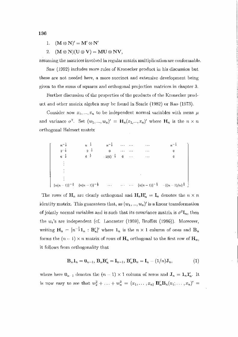
Consider now x1, ... , Xn to be independent normal variables with mean 1-L

and variance CJ2

. Set (w1, ... , wn)' Hn(x1, ... , Xn)' where Hn is the n x n

orthogonal Helmert matrix

_l I 1 I n 2 n -2 n -2 n -2

1 I 2-2 -2-2 0 0

I I -2(6)-! 6-2 6-2 0 0

I 1 {n(n -1)}-2 {n(n- 1)}-2 ...... {n(n-1)}-! -{(n-1)/n}!

The rows of Hn are clearly orthogonal and HnH~ = In denotes the n x n

identity matrix. This guarantees that, as (w1 , ... , wn)' is a linear transformation

of jointly normal variables and is such that its covariance matrix is CJ21n, then

the wi's are independent (cf. Lancaster (1959), Broffitt (1986)). Moreover,

writing Hn = [n-~ln : B~]' where ln is the n x 1 column of ones and Bn

forms the (n- 1) x n matrix of rows of Hn orthogonal to the first row of Hn,

it follows from orthogonality that

(1)

where here On_1 denotes the (n- 1) x 1 column of zeros and Jn = lnl~. It

is now easy to see that w~ + ... + w~ = (xt, ... , Xn) B~Bn(:ct·, ... , Xn)'

137

:Z::::(:ri- x) 2 = (n- 1)s;. Also 'WI = nhf. Since thew's are independent so are

- 1 2 x anc sn.

This illustration also described by Irwin, who acknowledges Burnside(1928)

as having also discovered it, is often given in the literature on recursive residu­

als. Here w2 , ... , Wn have mean zero. Addition of an extra normal observation

Xn+l easily leads to the construction of one new recursive residual 'Wn+l that

is independent ofw2 , ... , Wn previously calculated. The new estimate of vari­

ance s;+I = ((n 1)s; + w;+l)jn. They are referred to in Cox (1975) and

Fare brother (1987).

3. RANDOMISED COMPLETE BLOCK DESIGN

The observations from a randomisecl complete block design with r treat­

ments and s blocks are typically arranged in the following scheme

Blocks

1 2 s Means

Treatments

1 Yn Y12 Yts Yl.

2 y21 y22 Y2s Y2.

-r Y;.l 1~·2 Yrs Yr.

- -Means Y.1 Y.2 Y.s Y ..

The mathematical model for these data is

1'ij = p, + ai + (3j + eij , i = 1, ... , r; j = 1, · · · , s.

Here fl is the overall grand mean, ai is the i'th treatment effect, {3j is the j'th

block effect and the treatment and block effects satisfy restraints a. = (3. = 0

where a clot indicates summation over the index replaced by the dot. The errors

138

eij are independent normal variables with mean zero and variance a 2 . Express­

ing observations in the form of a vector Y = [Yn, ... , 1~·1, Y12, ... , Yr2, ... , Y1s,

... , 1";.8 ]', thereby ordering the columns of the table underneath each other, it

is easy to express the model as

Y = X,B+e (2)

where the vector ,8 = (J-t, a 1 , ... , an ,81 , ... , ,88 )', e is the vector of errors which

have the same indices as the elements ofY and the design matrix X is expressed

succinctly using Kronecker products as

(3)

An example of the derivation of such a design matrix can be found in Rogers

(1984, p.l98) for the two way model, though note that there observations are

ordered row by row from the two way table.

In essence Irwin(l934) expresses the treatment, block, and residual sums

of squares in terms of sums of squares of independent normal variables having

common variance a 2 . Thus,

1'

s L (}\ - i.Y = z~ + ... + z; i=l

s - -T L (1~j - Y . .)2 = z;+l + ... + z;+s-l

t=~ (1/· ·- 17. - 17 . + 17 )2- z2 + + z2 tSI f;:t tJ t. ·J .. - r+s · · · 1·s

(4)

-2 We include here the extra variable z? = rs Y .. to describe the correction for

the mean sum of squares. The vector z = (z1 , ... , Zrs)' is given here in matrix

notation by

eM (rs)-t1~ 01~.

z=CY= Cr

Y= s-t1~ 0 Br y (5)

CB r-tB 01' s r

CE Bs0Br

139

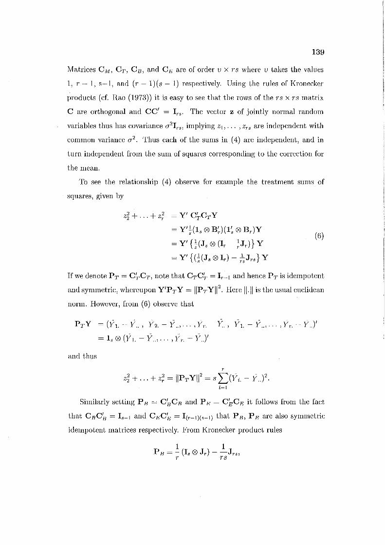
Matrices CM, Cr, C 8 , and CE are of order v x 7'3 where v takes the values

1, 7'- 1, s-1, and (7'- 1)(3- 1) respectively. Using the rules of Kronecker

r;roducts (cf. Rao (1973)) it is easy to see that the rows of the T3 x rs matrix

C are orthogonal and CC' = ITs· The vector z of jointly normal random

variables thus has covariance a 2I1's, implying z1 , ... , z1's are independent with

common variance a 2 . Thus each of the sums in ( 4) are independent, and in

turn independent from the sum of squares corresponding to the correction for

the mean.

To see the relationship (4) observe for example the treatment sums of

squares, given by

z~ + ... + z; = Y' C~Cr Y

= Y'~(ls ® B~)(l~ ® B~')Y

= Y' {~(Js ® (I1'- ~J1.)} Y

= Y' { (~(Js ® I1')- 1'1sJ1's} Y

(6)

If we denote Pr = C~Cr, note that CrC~ = I1'_1 and hence Pr is idempotent

and symmetric, whereupon Y'PrY = IIPr YW. Here 11.11 is the usual euclidean

norm. However, from (6) observe that

PTY = (}\.- Y .. , Y2.- Y .. , ... , Y1'.- Y., Yt.- Y .. , ... , Y1'.- Y .. )' - 1 ,'0, (171 - 17 17 - 17 )' - s '<Y • .. ' ••• ) 1'. ..

and thus

1' 2 2 2 "'"'- -2

Z2 + ... + z~' = IIPT Yll = s L...,.(Yi. - Y .. ) . i=1

Similarly setting P 8 = C~C8 and PE = C~CE it follows from the fact

that C8C~ = Is-1 and CEC~ = I(1'-1)(s-l) that P 8 , PE are also symmetric

idempotent matrices respectively. From Kronecker product rules

1 1 PB =-(Is® J1')- -J1·s,

r 7'3

140

and

whence the remaining two sums for (4) are simply IIPBYII2 and IIPEYII 2 re­

spectively.

Each Zi accounts for a degree of freedom. Consequently Irwin (1934) ob­

served that under the assumption of homogeneity (i.e. no treatment or block ef­

fect) that the variables z2 , •.• , z7•8 have zero mean, whence the sums of squares

of (4) are independent a2x2 with (r -1), (s -1), and (r -1)(s -1) degrees of

freedom. The matrix representation (5) allows us to arrive at the distributions

of these component sums of squares easily. in the more general situation of

non-zero treatment. and block effect parameters.

Considering E to be the linear expectation operator operating on each

element of a vector then

E[(z2, ... ,zr)'] = E[CrY] = CrE[Y] = CrXf3.

Observe from (3) and (5) and multiplication using Kronecker product rules

that

It follows from elementary distribution theory that the treatment sum of

squares given by (z2, ... , Zr)(z2, ... , Zr)' is distributed a2x;_hl where X;-bl , ,

is the noncentral chi-squared distribution on r - 1 degrees of freedom with

noncentrality parameter 8. Here

8 = (s/a2)(al, ... ,ar)B:.Br(o:l, ... ,ar)'

= (s/a2)(al, ... , O:r)(Ir- ~Jr)(o:1, · · · , ar)' 1'

= (s/a 2) 2::: az

i=l

141

Thus for example, the mean sum of squares for treatments has expectation r

cr2((r- 1) + 5)/(r- 1) = cr2 + (s/(r- 1)) I: af. Similar calculations for the . i=l

block sum of squares yield an expected vector E[(z,.+l, ... , Zr+s- 1)'] to be

whence the expected value for the mean block sum of squares is CJ2 + (r/(s-

s

1)) I: f3]. Since C EX is a matrix of zeros it follows that variables (zr+s, ... , ZTs) j=l

have mean zero and the residual sum of squares is distributed with central chi-

squared distribution cr2x(T-l)(s-l)'

A point which follows from the orthogonality of the matrix C is that

where here PM= c~[CM. This demonstrates the usual decomposition of the

sums of squares in the analysis of variance via

Y'Y =Y'(PM+Pr+PB+PE)Y

= IIPMYII2 + IIPrYII2 + IIPBYII2 + IIPEYII2

The orthogonal projection matrices PM, Pr, P B, P E yield unique compo­

nent sums of squares, whereas the choices of matrices Cr, CB and CE can

vary. We simply have made the choice suggested by Irwin (1934).

Interestingly, in the case of a randomised complete block design the recur­

sive residuals of Brown, Durbin and Evans (1975) can be shown to correspond

to the vector

This is established in Clarke and Godolphin (1992, Section 7). This highlights

the further historical link between the Helmert transformation and recursive

residuals, a link being earlier established by Farebrother (1978) to the work of

Pizzetti (1891).

142

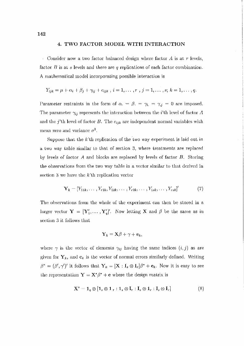
4. TWO FACTOR MODEL WITH INTERACTION

Consider now a two factor balanced design where factor A is at r levels,

factor B is at s levels and there are q replications of each factor combination.

A mathematical model incorporating possible interaction is

Yijk = Jl + ai + /3j + "/ij + eijk , i = 1, ... , r , j = 1, ... , s; k = 1, ... , q.

Parameter restraints in the form of a. = {3. = "/i. = "/.j = 0 are imposed.

The parameter "/ij represents the interaction between the i'th level of factor A

and the j'th level of factor B. The eijk are independent normal variables with

mean zero and variance CJ2

.

Suppose that the k'th replication of the two way experiment is laid out in

a two way table similar to that of section 3, where treatments are replaced

by levels of factor A and blocks are replaced by levels of factor B. Storing

the observations from the two way table in a vector similar to that derived in

section 3 we have the k 'th replication vector

The observations from the whole of the experiment can then be stored in a

larger vector Y = [Yi, ... , Y~]'. Now letting X and f3 be the same as in

section 3 it follows that

where ry is the vector of elements "/ij having the same indices ( i, j) as are

given for Y k, and ek is the vector of normal errors similarly defined. Writing

{3* = (/3', ry')' it follows that Y k = [X : Is ® Ir]/3* + ek. Now it is easy to see

the representation Y = X* /3* + e where the design matrix is

(8)

143

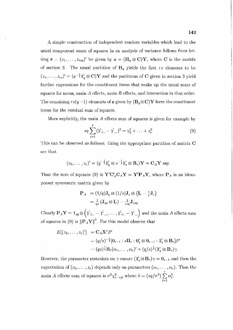
A simple construction of independent random variables which lead to the

usual component sums of squares in an analysis of variance follows from let­

ting z = (z1, ... , Zrsq) 1 be given by z = (Hq ® C)Y, where C is the matrix

of section 3. The usual partition of Hq yields the first rs elements to be

(z1 , ... , zTs)' = (q-~1~ ® C)Y and the partitions of C given in section 3 yield

further expressions for the constituent items that make up the usual sums of

squares for mean, main A effects, main B effects, and interaction in that order.

The remaining rs(q-1) elements of z given by (Bq®C)Y form the constituent

items for the residual sum of squares.

More explicitly, the main A effects sum of squares is given for example by 7'

sq :2)ii .. - i .. Y = ·z~ + ... + z?, (9) i=1

This can be observed as follows. Using the appropriate partition of matrix C

see that

Thus the sum of squares (9) is Y'CACA Y = Y'P A Y, where P A is an idem­

potent symmetric matrix given by

P A = (1/q)Jq ® (1/s)Js ® (17'- ~JT)

= 1_ (Jqs@ 17')- -1 JTSq qs rsq

Clearly PAY = 1sq ® ( Y 1.. - Y ... , . .. , Yr .. - 11- ... ) and the main A effects sum

of squares in (9) is liP A Yll 2. For this model observe that

E[(z2, ... , Zr)'] = CAX*(J*

= (q/st~[OT-1: sBT: 0~ ® Or-1: 1~ ® Br]fJ*

= (qs)~B7.(a1, ... , ar)' + (q/ s)~ (1~ ® Brh·

However, the parameter restraints on ry ensure ( 1 ~ ® Br )'y = 07'_1 and then the

expectation of (z2 , ... , z7') depends only on parameters (a1 , ... , aT). Thus the 7'

main A effects sum of squares is cr2x;-H where o = (sq/cr2) 2...:: aT. ' i=1

144

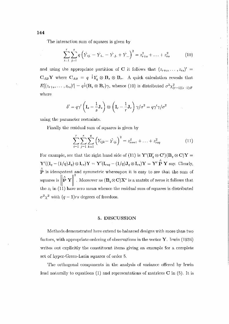
The interaction sum of squares is given by

Lr Ls ( - - - - )2 2 2

7 .. - 7. - 7 . 7 = z z q 1 tJ. 1 t.. 1 .J. + 1 ... 1·+s + · · · + rs (10) i=l j=l

and using the appropriate partition of C it follows that (zr+s, ... , z1•8 )1 =

CAB Y where CAB = q-11~ ® B 8 ® B 7•• A quick calculation reveals that

E[(zr+s, ... , ZrsY] = ql (Bs ® Br )'Y, whence (10) is distributed a2

x(r-l)(s-l);<>'

where

I I( 1 ) ( 1 ) I 2 I I 2 6 = qry Is - -; J s ® Ir - ;: J r '"'( a = qry '"'( a

using the parameter restraints.

Finally the residual sum of squares is given by

T s q

L L L ( 1~jk- iij.) 2

= z;s+l + · · · + z;sq (11) i=l j=l k=l

For example, see that the right hand side of (11) is Y1 (B~ ® C 1)(Bq ® C)Y = 1\

Y 1((Iq- (1lq)Jq) ® 11·s)Y = Y 1(1rsq- (1lq)Jq ® Irs)Y = Y 1 P Y say. Clearly, 1\ P is idempotent and symmetric whereupon it is easy to see that the sum of

squares is II p y r M oreovcr as ( Bq 0 c) X. is a matrix of ?.eros it fo !lows that

the Zi in (11) have zero mean whence the residual sum of squares is distributed

a 2x2 with (q- 1)rs degrees of freedom.

5. DISCUSSION

Methods demonstrated here extend to balanced designs with more than two

factors, with appropriate ordering of observations in the vector Y. Irwin (1934)

writes out explicitly the constituent items giving an example for a complete

set of hyper-Greco-Latin squares of order 5.

The orthogonal components in the analysis of variance offered by Irwin

lead naturally to equations (1) and representations of matrices C in (5). It is

145

not surprising that the arguments used in this article can be generalized to any

choice of matrix Bn satisfying equations (1). This is related to the question

of the representation of the error contrasts that one chooses to make. As has

been noted in Clarke and Godolphin (1992) the choice of Irwin leads to the

recursive residuals. In that paper it is shown that other choices of contrasts are

carrying an equivalent amount of information about a 2 and indeed about the

unobserved errors as they are orthogonal transformations of each other. This

is reinforced in this article in noting that regardless of the choice of matrices B

satisfying (1) the same sums of squares and orthogonal components in analysis

of variance are obtained. The sums of squares are, after all, unique. The de­

velopment of the current article highlights how the historical development of

the Helmert transformation can, along with Kronecker products, give simple

representations in analysis of variance leading to easy evaluation and interpre­

tation of distribution theory for some well known experimental designs. These

methods can be extended to more complicated designs.

ACKNOWLEDGEMENT

The author thanks Mr. Edward J. Godolphin for helpful comments and

the reference by Saw. The author thanks both Mr. Godolphin and Professor

Toby Lewis for the encouragement to pursue this publication.

BIBLIOGRAPHY

l.J.D. Broffitt, Zero correlation, independence, and normality, Amer. Statist.,

40 (1986), 276-277.

146

2.M.D. Brown, J. Durbin and J.M. Evans, Techniques for testing the constancy

of regression relationships over time, J.R. Statist. Soc. Ser. B, 37

(1975), 149-192.

3.W.Burnside, Theory of Probability, Cambridge Univ. Press, (1928).

4.B.R. Clarke and E.J. Godolphin, Uncorrelated residuals and an exact test

for two variance components in experimental design, Commun. Statist.

A Theory Methods, 21 (1992), 2501-2526.

5.W.G. Cochran, The distribution of quadratic forms in a normal system with

applications to the analysis of covariance, Proc. Camb. Phil. Soc., 30

(1934), 178-191.

6.D.R. Cox, In discussion of Techniques for testing the constancy of regression

relationships over time, by R.L. Brown, J. Durbin and J.M. Evans, J.R.

Statist. Soc. Ser. B, 37 (1975), 163-164.

7.R.W. Farebrother, An historical note on recursive residuals, J.R. Statist.

Soc., Ser. B, 40 (1978), 373-375.

8.R.W. Farebrother, N-dimensional geometry, Amer. Statist., 41 (1987), 242.

9.R.A. Fisher, Statistical Methods for Research Workers, Oliver, Edinburgh,

7th eel. (1938).

10.F.R. Helmert, Uber die Berechnung des wahrscheinlichen Fehlers aus einer

encllichen Anzahl wahrer Beobachtungsfehler, Z. Math. Phys., 20 (1875),

300-303.

11.F.R. Helmert, Die Genauigkeit der Formel von Peters zur Berechnung des

wahrscheinlichen Beo bachtungsfehlers directer Beo bachtungen gleicher

Genauigkeit, Astronom. Nachr., 88 (1876), 115-132.

12.R.R. Hocking, (1996) Methods and Applications of Linear Models Regres­

sion and the Analysis of Variance, Wiley, New York (1996).

147

13.J.O. Irwin, On the independence of constituent items in the analysis of

variance, J.R. Statist. Soc., Supplement 1 (1934) , 236-251.

14.H.O. Lancaster, Zero correlation and independence, Austral. J. Statist.,

21 (1959), 53-56.

15.H.O. Lancaster, The Helmert matrices, Amer. Math. Month., 72 (1965),

4-12.

16.P. Pizzetti, I Fondamenti Matmematici per la Critica dei Risultati Sper­

imentali, Genoa. (1891),Reprinted in Atti della Universita di Geniova,

(1892).

17.C.R. Rao, Linear statistical infeTence and its applications, Wiley, New York,

2nd eel. (1973).

18.G.S. Rogers, Kronecker products in ANOVA-A first step, AmeT. Statist.,

38 (1984), 197-202.

19.S.L.C. Saw, ANOVA sums of squares as quadratic forms, Amer. Statist.,

46 (1992)' 288-290.

20.S.R. Searle, Linear models, Wiley, New York (1971).

2l.S.R. Searle, Matrix algebra useful for statistics , Wiley, New York (1982).

Received: October 30, 2000

International Mathematical Journal

Aims and scopes: The journal will publish carefully selected original

research papers in the area of pure and applied mathematics as follows:

combinatorics, order, lattices, ordered algebraic structures, general

mathematical systems, number theory, field theory and polynomials,

commutative rings and algebras, algebraic geometry, linear and multi linear

algebra, matrix theory, associative and nonassociative rings, category theory,

homological algebra, K - theory, group theory, Lie algebras, real functions,

measure and integration, functions of complex variables, potential theory,

special functions, ordinary differential equations, partial differential

equations, finite difference and functional equations, approximation and

expansion, Fourier analysis, abstract harmonic analysis, integral transforms,

operational calculus, integral equations, functional analysis, operator theory,

calculus of variation and optimal control, optimization, geometry,

differential geometry, topology, manifolds, probability theory and stochastic

processes, statistics, numerical analysis, computer science, mechanics,

thermodynamics, quantum theory, relativity, economics, programming,

games, mathematical biology, information and communication, circuits.

Call for papers: The authors are cordially invited to submit papers in

triplicate to the Managing Editor: Emil Minchev. Manuscripts submitted to

this journal will be considered for publication with the understanding that

the same work has not been published and is not under consideration for

publication elsewhere.

Managing Editor: Dr. Emil Minchev, Department of Mathematics,

Faculty of Education, Chiba University, Yayoi- cho 1-33, lnage- ku,

Chiba 263-8522, Japan

e - mail: eminchev@hotmail.com

International Mathematical Journal, Vol. 1, no. 2, 2002

Contents

J. J. Shepherd, H. J. Connell, Helical flow of a power law fluid

between coaxial cylinders with small radial separation . . . . . . . . . . . . . 105

B. R. Clarke, A representation of orthogonal components in analysis

of variance 133

L. M. Batten, Decompositions of finite projective planes 149

T. - S. Kim, H. Ch. Kim, A functional central limit theorem for the

multivariate linear process generated by associated random vectors 161

M.S. Metwally, On the generalized Hadamard product functions

of two complex matrices 171

D. Applebaum, On the subordination of spherically symmetric

Levy processes in Lie groups 185

Tadie, Radial solutions of some mixed singular and non singular

elliptic equations .. .. . .. . .. . .. . .. . .. . .. . .. . .. . .. . .. . .. . .. . .. . .. . .. .. .. .. . .. . .. . .. 195

E. Ballico, Pairs of meromorphic vector fields on projective spaces

and stability ...................................... ; . . . . . . . . . . . . . . . . . . . . . . . . . . . . . . 205