orthogonal support vector machine for credit scoring · the most commonly used techniques for...

Engineering Applications of Artificial Intelligence 26 (2013) 848–862

Contents lists available at SciVerse ScienceDirect

Engineering Applications of Artificial Intelligence

0952-19

http://d

n Corr

E-m

hongwe

journal homepage: www.elsevier.com/locate/engappai

Orthogonal support vector machine for credit scoring

Lu Han a,b,n, Liyan Han a, Hongwei Zhao b

a School of Economics and Management, Beihang University, Beijing 100191, Chinab PBC School of Finance, Tsinghua University, Beijing 100083, China

a r t i c l e i n f o

Article history:

Received 8 December 2011

Received in revised form

25 September 2012

Accepted 8 October 2012Available online 17 November 2012

Keywords:

Dimension curse

Orthogonal dimension reduction

Support vector machine

Logistic regression

Principal component analysis

Credit scoring

76/$ - see front matter Crown Copyright & 2

x.doi.org/10.1016/j.engappai.2012.10.005

esponding author. Tel.: þ86 1861 166 7963.

ail addresses: [email protected] (L. Han), ha

[email protected] (H.W. Zhao).

a b s t r a c t

The most commonly used techniques for credit scoring is logistic regression, and more recent research

has proposed that the support vector machine is a more effective method. However, both logistic

regression and support vector machine suffers from curse of dimension. In this paper, we introduce a

new way to address this problem which is defined as orthogonal dimension reduction. We

discuss the related properties of this method in detail and test it against other common statistical

approaches—principal component analysis and hybridizing logistic regression to better solve and

evaluate the data. With experiments on German data set, there is also an interesting phenomenon with

respect to the use of support vector machine, which we define as ‘Dimensional interference’, and

discuss in general. Based on the results of cross-validation, it can be found that through the use

of logistic regression filtering the dummy variables and orthogonal extracting feature, the support

vector machine not only reduces complexity and accelerates convergence, but also achieves better

performance.

Crown Copyright & 2012 Published by Elsevier Ltd. All rights reserved.

1. Introduction

Credit risk based on the characteristics of the debtor is oftendivided into sovereign, corporate, retail, etc. Retail debt is cen-tered on customer credit, which includes short-term andintermediate-term credit to finance the purchase of commoditiesand services for consumption or to refinance debt incurred forsuch purposes. Retail credit is characterized by three points: first,large amounts with small scale. At present in China, retail loanscan account for a quarter of the total debt, with a speed of growthapproaching 10%; second, the potential risk is high but theinformation is scattered and complicated. In the loan applicationform there are thousands of variables to describe and, even worse,is that different organizations always use different variables; andthird, the efficiency of business processing requires highly devel-oped decision-making techniques as competition is getting moreand more intense. These characteristics determine the banks needto implement risk management evaluation methods based onquantitative analysis. A good credit risk evaluation tool can helpto grant credit to more creditworthy applicants and thusincreases profit. Moreover, it can deny credit for the noncreditworthy applicants and thus decreases losses.

Currently, credit scoring has become the primary method todevelop a credit risk assessment tool. It is a method to evaluate

012 Published by Elsevier Ltd. All

[email protected] (L.Y. Han),

the credit risk of loan applicants with their corresponding creditscore that is obtained from a credit scoring model (Altman, 1998).A credit score is a number that can represent the creditworthinessof an applicant and it is based on the analysis of an applicant’scharacteristics from the application file using the credit scoringmodel. The credit scoring model (Thomas et al., 2002) is devel-oped on the basis of historical data about the applicant’s perfor-mance on previously made loans with the use of somequantitative techniques, such as statistics analysis, mathematicalprogramming, artificial intelligence and data mining. A well-designed model should have higher classification accuracy toclassify the new applicants or existing customers as good or badand the model is the core of credit scoring.

The most popular methods adopted in credit scoring arestatistical methods. The statistical principle discriminating differ-ent groups in a population can be traced back to 1936 in Fisher(1936) publication which used a linear model to calculate thedistance between two classes as the decision factor. It is known asthe Fisher’s discrimination model. In 1977, Martin (1977) firstintroduced the logistic regression method to the bank crisis earlywarning classification. Martin chose to use data between 1970and 1976, with 105 bankrupt companies and 2058 non-bankruptcompanies in the matching sample, and analyzed the bankruptcyprobability interval distribution, with two types of errors and therelationship between the split points, he then found that size,capital structure, and performance were key indexes for thejudgment. Martin determined that the accuracy rate of the overallclassification could reach 96.12%. Logistic regression analysis had

rights reserved.

www.elsevier.com/locate/engappai

www.elsevier.com/locate/engappai

dx.doi.org/10.1016/j.engappai.2012.10.005



mailto:[email protected]




L. Han et al. / Engineering Applications of Artificial Intelligence 26 (2013) 848–862 849

significant improvements over discriminant analysis with respectto the problem of classification. Martin also noted that logisticregression could overcome many of the issues with discriminantanalysis, including the assumption that variables must be nor-mally distributed. Wiginton (1980), was one of the first research-ers to report credit scoring results with the logistic regressionmodel. Although the result was not very impressive, the modelwas simple and could be illustrated easily. Then, at that point thelogistic regression model had become the main approach for thepractical credit scoring application. In 1997, Hand and Henley(1997) summarized statistical methods in credit scoring. Thesemethods are relatively easy to implement and are able to generatestraightforward results that can be readily interpreted. None-theless, as commonly known, there are also quite a few limita-tions associated with the applications of these statistical methods.First of all, they have the fatal problem called ‘Curse of dimension’which suggests that if there are numerous variables to apply,because of multicollinearity between variables, the results arealways erroneous and misleading. Therefore, before applyingstatistical methods, the process entailed tremendous data pre-processing efforts through variable selection. This strategy usuallyrequires domain expert knowledge and an in-depth understand-ing of the data. In addition, all the statistical models are based ona hypothesis condition. In a real world application, a hypothesissuch as that the dependent variable should follow logic normaldistribution and so on, may not hold. Most importantly, based onthese algorithms, these statistical models have difficulty in theautomation of modeling processes and lack robustness. Whenenvironmental or population changes occur, the static modelsusually fail to adapt and need to be rebuilt again.

In response to the concern for classification accuracy in retailloans applications, researchers discovered the application of thesupport vector machine (SVM). The support vector machines(SVM) approach was first proposed by Cortes and Vapnik(1995). The main idea of SVM is to minimize the upper boundof the generalization error. SVM usually maps the input variablesinto a high-dimensional feature space through some nonlinearmapping. In that space, an optimal separating hyper plane, whichis one that separates the data with the maximal margin, isconstructed by solving a constrained quadratic optimizationproblem. Suykens et al. (2002) constructed the least squaressupport vector machine(LS-SVM) and used it for the credit ratingof banks and reported the experimental results compared withordinary least squares (OLS), ordinary logistic regression (OLR)and the multilayer perceptron (MLP). The result showed that theaccuracy of the LS-SVM classifier was better than the other threemethods. Schebesch and Stecking (2005) used a type of standardSVM proposed by Vanik with a linear and radial basis function(RBF) kernel for dividing credit applicants into subsets of ‘typical’and ‘critical’ patterns which can be used for rejecting applicants.Schebesch and Stecking concluded these types of SVM should bewidely used because of their performance. Gestel et al. (2003)discussed a benchmark study of seventeen different classificationtechniques on eight different real-life credit datasets. They usedSVM and LS-SVM with linear and RBF kernels and adopted a gridsearch mechanism to tune the hyper parameters in their study.The experimental results indicated that six different methodswere the best in terms of classification accuracy among the eightdatasets — linear regression, logistic regression, linear program-ming, classification tree, neural networks and SVM. In addition,the experiments showed that the SVM classifiers can overall yieldthe best performance. Yang (2007) experimented with severalkernel learning methods to apply adaptive credit scoring, andfound that the results can be very impressive when using theSVM. Nevertheless the existing research findings have all focusedon batch learning and the selection of parameters, as seen in the

work of Yu et al. (2006,2008) which shows SVM’s advantages insolving high dimensional problems. However, there are twoobvious drawbacks to SVM (Min and Lee, 2005). One is that whenthe variables are not ‘meaningful’ and ‘huge’, SVM requires a longtime to train and the hyper plane is not accurate, which we alsodefine as curse of dimension. The drawback is a fatal flaw,although this method has good robustness and can alwaysachieve higher accuracy, when applied to samples, SVM lacksthe capability to explain its results. That is, the results obtainedfrom SVM classifiers are not intuitive to humans and are difficultto illustrate comparing with logistic regression. This is a commonproblem that all machine learning methods are facing. Though theresults with these methods have strong advantages in accuracy,the non-parameter results often lack of statistical theory, and sowhich cannot be directly corresponding to the realistic economicsignificance. Just as in regression analysis, regression coefficientdirectly represents the influence of independent variable actingon dependent variable, but in support vector machine (SVM), therelationship between independent variable and dependent vari-able cannot be explained directly. So this limits these methods inpractical application, and at the same time this also is a cause forover fitting phenomenon.

Dimension curse (Anderson, 1962) can be defined as thisphenomenon: as the number of variables increase, more andmore variables will have multicollinearity, which can bedescribed as when the correlation coefficient gets large, and isin a high dimensional space, the distribution of the sample pointswill become sparse. Statistical methods will prove to be erroneouswith multicollinearity, and SVM will need a large amount ofsupport vectors to construct hyper plane. Now, to solve the curseof dimensionality, researchers often use two methods to reducevariables. One method is feature selection, another is featureextraction. Feature selection is to select important variablesclosely related with the target in order to reduce the model’sdimensions; feature extraction is to construct new variableswhich are not linearly dependent through structure transforma-tion. The drawback of feature selection is in reducing informationand the advantage is that it is easy to explain. Feature extractionis just the opposite. Many scholars have performed a lot of workto reduce dimensions. Sugiyama (2007) tried feature selection toreduce dimensions in Fisher discriminant analysis. Bellman(1961) is the first to note the curse of dimension in kernelclassifiers. He stipulated that owing to the large amounts of datafrom public financial statements that can be used for bankruptcypredictions, the large scale of input data makes Kernel classifiersinfeasible due to the curse of dimensionality. Consequently, oneneeds to transform the input data space to a suitable lowdimensional subspace that optimally represents the data struc-ture. In the studies of Huang (2009), he discussed the use of anonlinear graph as a type of method for feature selection toreduce dimension. Han and Han (2010) have tried logisticregression to select meaningful variables for neural networks.The other methods regarding dimensionality reduction, linearalgorithms such as principal component analysis and lineardiscriminant analysis, are the two most widely used methods,which can be found in the works of Gutierrez et al. (2010) andHua et al. (2007).

Just based on the studies above, we want to improve theaccuracy of credit scoring through dimension reduction. Ournovel contribution is that we give these researchers in the fieldof application using logistic regression and support vectormachine a new way to address dimension curse that we definedas ‘Orthogonal dimension reduction’ (ORD). Based on the experi-ence of statistics, we compare the traditional way to addressdimension curse—hybridizing with logistic regression (HLR)(Fukunaga, 1990) on behalf of feature selection and principal

L. Han et al. / Engineering Applications of Artificial Intelligence 26 (2013) 848–862850

component analysis (PCA) (Jolliffe, 2002) on behalf of featureextraction. Then, we fit these helpful features chosen by ORD, HLRand PCA in logistic regression and support vector machine toevaluate the accuracy of credit scoring. Furthermore, we comparethese results with the original methods without reducing dimen-sion. Finally, we acquire cross-validation to make the resultssensitive.

The structure of the rest in this paper is as follows: the nextsection puts forward the prior research of logistic regression andsupport vector machine. Section 3 briefly summarizes the pre-vious methods of reducing dimension. Section 4 describes ourmethod of orthogonal dimension reduction and its main princi-ples in detail. Section 5 is about experiment design, including dataand variable description, data pre-processing, evolutionary learn-ing for SVM, features selection with HLR, features extraction withPCA and ODR, cross-validation design, and accuracy criterion.Experimental studies using the original methods and the methodshybridizing dimension reduction are presented in Section 6. TheFinal section discusses the interesting results and gives someremarks.

Margin=2/ |w|

Fig. 1. Separating hyperplane for two separable classes.

2. Prior research

Let X ¼ x1,x2, � � � xnð ÞT be a set of n random variables which

describe the information from a customer’s application form andcredit reference bureau. The actual value of the variables for aparticular applicant i is denoted by Xi ¼ x1i,x2i, � � � xnið Þ

T . All sam-ples denoted by S¼ Xi,yi

� �,i¼ 1,2, � � � ,N, where N is the number of

samples, Xi is the attribute vector of the ith customer, and yi is itscorresponding observed result of timely repayment. If the custo-mer is good, yi¼1, else yi¼�1. Let I¼{i9yi¼1,iAN,(xi,yi)AS} is onbehalf of good customers, J¼{i9yi¼�1,iAN,(xi,yi)AS} is on behalfof bad ones.

Though in practice a credit scoring result needs the score ofeach applicant, in fact our greatest concern is the accuracy of thedistinction between categories. Thus, the credit scoring problemcan be described simply as making a classification of good or badfor a certain customer using the attribute characteristics of acertain customer. That is, using the attribute vector Xk, one canjudge the credit status. The typical credit risk modeling techni-ques, which were tested in this paper, are briefly described below.

2.1. Logistic regression

Just as linear regression, logistic regression assumes that thesum of the weighted input variables is linearly correlated to thenatural log of the odds that the outcome event will happen. It canbe described as (1):

log p=1�p� �

¼ b1x1þb2x2þ . . .þbkxkþe¼ bT Xkþe ð1Þ

where b¼(b1,b2,yy,bk) is the vector of the coefficients of themodel, the maximum likelihood method can be applied tocompute the estimate of bi i¼ 1,2 � � � k

� �. We refer to p/(1�p)

as odds-ratio and assume the regression model in (1) is obtained,the estimated probability of no default is as follows:

p¼eb

T x

1þebT x

ð2Þ

Linear regression is based on the idea of using vector X toexplain y logistic regression is the same, using X to explain naturallog of the odds, so just like linear regression, it has goodinterpretations in statistical sense. But logistic regression canovercome the flaw of linear regression, which is that the right sideof the model could take any value from �N to þN but the leftside can only take values between 0 and 1.

The method has two shortcomings: one is that it can onlyexplain the intrinsically linear relationship, and cannot addressnon-linear effects in practice. Researchers always explain anynon-linear effects with variable combinations and this requiresseveral repetitions of a trial-and-error process. In addition, themethod is sensitive to redundancy or collinearity in the inputvariables to guarantee the basic assumption of e, which isei �NID 0,s2

� �, which therefore requires that y obey logic normal

distribution. If this condition is not satisfied, this method will giveerroneous estimates of the coefficients and is not valid forstatistical interpretation.

2.2. Support vector machine

The main idea of support vector machine is to minimize theupper bound of the generalization error not the empirical error.Without loss of generality, in a two-dimensional space, if thesescoring samples are linear separable, The upper bound can beconstructed by (wx)þb¼1 and (wx)þb¼�1, so a decision func-tion can be created to specify whether a given application belongsto either I or J. Its definition is as follow: f(x)¼sign((wx)þb).While the vector w defines the boundary, in order to get the twoupper bound separated as far as possible, the optimal hyperplanecan be obtained as a solution to the optimization problem:

max 2JwJ2

s:t:

yi wUxið ÞþbÞZ1 i¼ 1,2, � � �n� ð3Þ

which could be written as (4):

min 12 JwJ2

s:t:

yi wUxið ÞþbÞZ1 i¼ 1,2, � � �n� ð4Þ

So an optimal separating hyperplane which is one thatseparates the data with the maximal margin is constructed bysolving a constrained quadratic optimization problem whosesolution has an expansion in terms of a subset of training patternsthat lie closet to the boundary, and this subset of patterns arecalled as support vector (SV). Fig. 1 shows such a hyperplane thatseparate two classes to the boundary.

In many practical situation, the training samples cannot belinear separable. There is a need to use soft margin and C penaltyparameters, this is formulized as the following constraint opti-mization problem:

min J w,b,xkð Þ ¼ 12 JwJ2

þCP

kxk

s:t:

yi wUxið ÞþbÞZ1 i¼ 1,2, . . .nxkZ0� ð5Þ

where C is the corresponding penalty parameters indicating atradeoff between large margin and a small number of margin


failures: few errors are permitted for high C, while low C allows ahigher proportion of errors in the solution. The solution to thisoptimization problem can be given by the saddle point of theLagrange function with Lagrange multipliers ai, and then theproblem can be transformed into its dual form:

max J að Þ ¼ � 12

Pk

Plakalykyl/xkUxlSþ

Pkak

s:t:Pkakyk ¼ 0,

yk ¼ 1,kA I

yk ¼�1,kA J0rakrC, 8k

( ð6Þ

In cases where the linear boundary in input spaces is not beable to separate the two classes accurately, a hyperplane iscreated that allows linear separation in the higher dimension bythe use of transformation function j(U) which can map the inputspace into a higher dimensional feature space (z-space), then theobjective function can be rewritten as:

max J að Þ ¼�1

2

Xk

Xlakalykyl/j xkð Þj xlð ÞSþ

Xkak ð7Þ

But using this way to transformation is relatively compu-tation-intensive. And we can find j(U) only uses for inner product,therefore a kernel can be used to perform this transformation andthen inner product can be replaced by kernel function which isgiven by Mercer’s theorem. The kernel function is defined as (8):

K x,yð Þ ¼jðxÞjðyÞ ð8Þ

The most common kernel functions are listed below.

(1)

x

Linear kernel function: K xk,xð Þ ¼ xTk x� �

(2)
Polynomial function: K xk,xð Þ ¼ xTk xþ1
d� �
(3) Gaussian function: K xk,xð Þ ¼ exp �Jxk�xJ2=s2
2 2� �

(4)
Radial basis kernel: K xk,xð Þ ¼ exp �Jxk�xJ =2s
Then the objective function can be rewritten as:

max J að Þ ¼ � 12

Pk

PlakalykylK xk,xlð Þþ

Pkak

s:t:Pkakyk ¼ 0,

yk ¼ 1,kA I

yk ¼�1,kA J0rakrC,8k

( ð9Þ

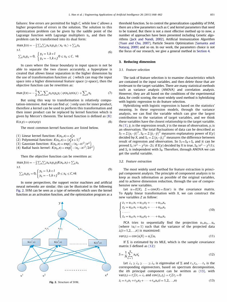
In some perspectives, the support vector machines and artificialneural networks are similar; this can be illustrated in the followingFig. 2. SVM can be seen as a type of networks which uses the kernelfunction as an activation function, and the optimization program as a

1 x2 xd

…………

K(x1,x) K(x2,x) K(xd,x)…………

y

a1y1 a2y2 a3y3

Fig. 2. Structure of SVM.

threshold function. So to control the generalization capability of SVM,there are a few parameters such as C and kernel parameters that needto be trained. But there is not a most effective method up to now, anumber of approaches have been presented including Genetic algo-rithms (Jack and Nandi, 2002), Artificial Immunization Algorithm(Yuan and Chu, 2007), Particle Swarm Optimization (Samanta andNataraj, 2009) and so on. In our work, the parameters choice is notthe focus of our research, we give a general method in Section 4.

3. Reducing dimension

3.1. Feature selection

The task of feature selection is to examine characteristics whichare contained in the input variables, and then delete those that areirrelevant to the target variables. There are many statistical methodssuch as variance analysis (ANOVA) and correlation analysis.However, they are all based on the conditions of the experimentaldata, for credit scoring, the most widely used method is hybridizingwith logistic regression to do feature selection.

Hybridizing with logistic regression is based on the statistics’meaning. In these regression models, through the varianceanalysis, we can find the variable which can give the largestcontribution to the variation of target variables, and we thinkthese variables have the closest relationship to the target variable.As (1), yi is the regression result, y is the mean of observation, yi isan observation. The total fluctuations of data can be described asST ¼S yi�y

� �2, SR ¼S yi�y

� �2measures explanatory power of E(y)

decided by X, and Se ¼S yi�yi

� �2measures the difference between

result of regression and observation. So ST¼SRþSe and it can beproved Se=s2 � w2 n�2ð Þ; if E(y) decided by X is true, SR=s2 � w2ð1Þ;and Se is independent with SR. Therefore, through ANOVA we canget the useful variable.

3.2. Feature extraction

The most widely used method for feature extraction is princi-pal component analysis. The principle of component analysis is tokeep as much information as possible of the original variables,and to achieve dimension reduction, through the use of compre-hensive new variables.

Let u¼E(X), S¼ covðXÞ ¼ E xx0ð Þ is the covariance matrix.To Apply linear transformation with X, we can construct thenew variables Z as follow:

z1 ¼ u11x1þu12x2þ � � � þu1nxn

z2 ¼ u21x1þu22x2þ � � � þu2nxn

. . .. . .

zn ¼ un1x1þun2x2þ � � � þunnxn

8>>><>>>:

ð10Þ

PCA tries to sequentially find the projection u1,u2,yun

(where JuiJ¼ 1) such that the variance of the projected datazi(i¼1,2,y,n) is maximized:

var zið Þ ¼ cov u0iX� �

¼ u0iSui ð11Þ

If S is estimated by its MLE, which is the sample covariancematrix S defined as (12):

S¼1

N

XN

k ¼ 1

xkx0k ð12Þ

Let l1Zl2Z � � �Zln is eigenvalue of S and r1,r2, � � � rn is thecorresponding eigenvectors, based on spectrum decomposition,the ith principal component can be written as (13), withvar zið Þ ¼ r0iSri ¼ li and cov zi,zj

� �¼ r0iSrj ¼ 0

zi ¼ r1ix1þr2ix2þ � � � þrnixn i¼ 1,2,. . .,nð Þ ð13Þ


4. Orthogonal dimension reduction

In this section we give a new method to do feature extraction.The step of transform is described as (14):

z1 ¼ x1

z2 ¼ x2�x0

2z1

x01z1

z1

z3 ¼ x3�x0

3z1

x01z1

z1�x0

3z2

x02z2

z2

� � � � � �

zs ¼ xs�Xs�1

i ¼ 1

x0szi

x0izizi

ð14Þ

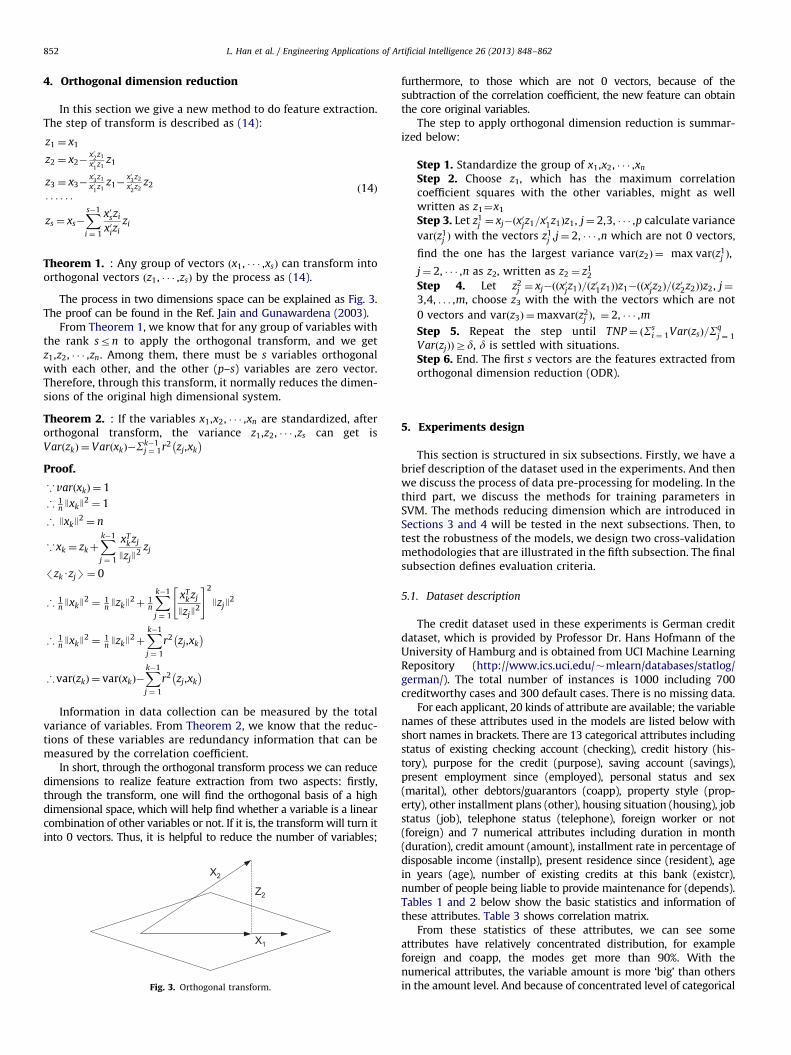
Theorem 1. : Any group of vectors x1, � � � ,xsð Þ can transform intoorthogonal vectors z1, � � � ,zsð Þ by the process as (14).

The process in two dimensions space can be explained as Fig. 3.The proof can be found in the Ref. Jain and Gunawardena (2003).

From Theorem 1, we know that for any group of variables withthe rank srn to apply the orthogonal transform, and we getz1,z2, � � � ,zn. Among them, there must be s variables orthogonalwith each other, and the other (p–s) variables are zero vector.Therefore, through this transform, it normally reduces the dimen-sions of the original high dimensional system.

Theorem 2. : If the variables x1,x2, � � � ,xn are standardized, afterorthogonal transform, the variance z1,z2, � � � ,zs can get isVar zkð Þ ¼ Var xkð Þ�S

k�1j ¼ 1r2 zj,xk

� �Proof.

_var xkð Þ ¼ 1

‘ 1n JxkJ

2¼ 1

‘ JxkJ2¼ n

_xk ¼ zkþXk�1

j ¼ 1

xTk zj

JzjJ2

zj

/zkUzjS¼ 0

‘ 1n JxkJ

2¼ 1

n JzkJ2þ 1

n

Xk�1

j ¼ 1

xTk zj

JzjJ2

" #2

JzjJ2

‘ 1n JxkJ

2¼ 1

n JzkJ2þXk�1

j ¼ 1

r2 zj,xk

� �

‘var zkð Þ ¼ var xkð Þ�Xk�1

j ¼ 1

r2 zj,xk

� �

Information in data collection can be measured by the totalvariance of variables. From Theorem 2, we know that the reduc-tions of these variables are redundancy information that can bemeasured by the correlation coefficient.

In short, through the orthogonal transform process we can reducedimensions to realize feature extraction from two aspects: firstly,through the transform, one will find the orthogonal basis of a highdimensional space, which will help find whether a variable is a linearcombination of other variables or not. If it is, the transform will turn itinto 0 vectors. Thus, it is helpful to reduce the number of variables;

X2

X1

Z2

Fig. 3. Orthogonal transform.

furthermore, to those which are not 0 vectors, because of thesubtraction of the correlation coefficient, the new feature can obtainthe core original variables.

The step to apply orthogonal dimension reduction is summar-ized below:

Step 1. Standardize the group of x1,x2, � � � ,xn

Step 2. Choose z1, which has the maximum correlationcoefficient squares with the other variables, might as wellwritten as z1¼x1

Step 3. Let z1j ¼ xj�ðx

0jz1=x01z1Þz1, j¼ 2,3, � � � ,p calculate variance

varðz1j Þ with the vectors z1

j ,j¼ 2, � � � ,n which are not 0 vectors,

find the one has the largest variance var z2ð Þ ¼ max varðz1j Þ,

j¼ 2, � � � ,n as z2, written as z2 ¼ z12

Step 4. Let z2j ¼ xj�ððx

0jz1Þ=ðz

01z1ÞÞz1�ððx

0jz2Þ=ðz

02z2ÞÞz2, j¼

3,4, . . . ,m, choose z3 with the with the vectors which are not

0 vectors and var z3ð Þ ¼maxvarðz2j Þ, ¼ 2, � � � ,m

Step 5. Repeat the step until TNP¼ ðSsi ¼ 1VarðzsÞ=Sq

j ¼ 1

VarðzjÞÞZd, d is settled with situations.Step 6. End. The first s vectors are the features extracted fromorthogonal dimension reduction (ODR).

5. Experiments design

This section is structured in six subsections. Firstly, we have abrief description of the dataset used in the experiments. And thenwe discuss the process of data pre-processing for modeling. In thethird part, we discuss the methods for training parameters inSVM. The methods reducing dimension which are introduced inSections 3 and 4 will be tested in the next subsections. Then, totest the robustness of the models, we design two cross-validationmethodologies that are illustrated in the fifth subsection. The finalsubsection defines evaluation criteria.

5.1. Dataset description

The credit dataset used in these experiments is German creditdataset, which is provided by Professor Dr. Hans Hofmann of theUniversity of Hamburg and is obtained from UCI Machine LearningRepository (http://www.ics.uci.edu/�mlearn/databases/statlog/german/). The total number of instances is 1000 including 700creditworthy cases and 300 default cases. There is no missing data.

For each applicant, 20 kinds of attribute are available; the variablenames of these attributes used in the models are listed below withshort names in brackets. There are 13 categorical attributes includingstatus of existing checking account (checking), credit history (his-tory), purpose for the credit (purpose), saving account (savings),present employment since (employed), personal status and sex(marital), other debtors/guarantors (coapp), property style (prop-erty), other installment plans (other), housing situation (housing), jobstatus (job), telephone status (telephone), foreign worker or not(foreign) and 7 numerical attributes including duration in month(duration), credit amount (amount), installment rate in percentage ofdisposable income (installp), present residence since (resident), agein years (age), number of existing credits at this bank (existcr),number of people being liable to provide maintenance for (depends).Tables 1 and 2 below show the basic statistics and information ofthese attributes. Table 3 shows correlation matrix.

From these statistics of these attributes, we can see someattributes have relatively concentrated distribution, for exampleforeign and coapp, the modes get more than 90%. With thenumerical attributes, the variable amount is more ‘big’ than othersin the amount level. And because of concentrated level of categorical

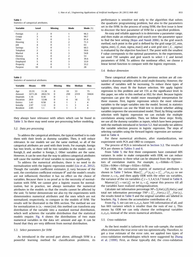
http://www.ics.uci.edu/~mlearn/databases/statlog/german/



Table 1Statistics of categorical attributes.

Variable Level Missing Mode Mode (%)

Foreign 2 0 1 96.3

Coapp 3 0 1 90.7

Other 3 0 3 81.4

Housing 3 0 2 71.3

Job 4 0 3 63

Savings 5 0 1 60.3

Telephon 2 0 1 59.6

Marital 4 0 3 54.8

History 5 0 2 53

Checking 4 0 4 39.4

Employed 5 0 3 33.9

Property 4 0 3 33.2

Purpose 10 0 3 28

Table 2Statistics of numerical attributes.

Variable Means STD Missing Min Median Max

Age 35.55 11.38 0 19 33 75

Amount 3271.26 2822.74 0 250 2319 18424

Depends 1.16 0.36 0 1 1 2

Duration 20.9 12.06 0 4 18 72

Existcr 1.41 0.58 0 1 1 4

Installp 2.97 1.12 0 1 3 4

Resident 2.85 1.1 0 1 3 4


they always have relevance with others which can be found inTable 3. So there may need some pre-processing before modeling.

5.2. Data pre-processing

To address the categorical attributes, the typical method is to codethem with their levels as dummy variables. Then, it will reducerelevance. In our models we use the same method, so all of thecategorical attributes are used with their levels. For example, foreignhas two levels, so there will be two variables in the model—one isforeigh_0, and another is foreign_1. Other variables are the same.However, it can be seen that the way to address categorical attributeswill cause the number of total variables to increase significantly.

To address the numerical attributes, there is no need to donormalization with the logistic regression model (Liu et al., 2012).Though the variable coefficient estimates bi vary because of theunit, the correlation coefficient estimate R2 and the model’s resultsare not influenced, therefore it has no effect on the choice ofvariables. Because there is no proof as to the necessity of normal-ization with SVM, we cannot give a logistic reason for normal-ization, but in practice, we always normalize the numericalattributes in the models so that the results cannot be affected bythe unit. To better demonstrate we also try the experiments withdimensionless numerical attributes and the ones which are notnormalized, respectively, to compare in the models of SVM. Theresults will be illustrated in the fifth section. The method we usefor normalization is (xi�mean)/std, this method can transform anydistribution of the variable into a standard normal distribution,which well achieves the variable distribution that the statisticalmodels require. Fig. 4 shows the distributions of two mainnumerical variables in the data set: amount and age. It can befound that they are very different from normal distribution.

5.3. Select parameters for SVM

As introduced in the second part above, although SVM is apowerful learning method for classification problems, its

performance is sensitive not only to the algorithm that solvesthe quadratic programming problem, but also to the parametersset in the SVM. In the process of using SVM, the first issue is howto discover the best parameter of SVM for a specified problem.

An easy and reliable approach is to determine a parameter range,and then make an exhaustive grid search over the parameter spaceto find the best setting (Rojas and Nandi 2006). In the grid searchmethod, each point in the grid is defined by the grid range [(C_min,sigma_min), (C_max, sigma_max)] and a unit grid size (_C, _sigma)is evaluated by the objective function F. The point with the smallestF value corresponds to the optimal parameters. In the experiments,we used 750 samples and gird search to select t C and kernelparameters of SVM. To address the nonlinear effect, we choose alinear kernel function to compare with the logistic regression.

5.4. Reduce dimension

These categorical attributes in the previous section are all con-tained in dummy variables which avoid multi-linearity. However, thenumber of variables will be increasing. To reduce these types ofvariables, they must fit the feature selection. We apply logisticregression to this problem and set 15% as the significance level. Inthis paper, we refer to this method as HLG for short. Because logisticregression can give the model more meaningful interpretation forthree reasons. First, logistic regression selects the most relevantvariables to the target variables into the model. Second, in statisticslogistic regression can use the Wald test to decide whether addingvariables improves the unconstrained model. Third, by fitting variableselection with logistic regression we can exclude the multiplecorrelations among variables. Then, we follow these steps: firstly,we use all the dummy variables as inputs, which have been preparedwith the methods introduced in Section 5.2. And secondly we addressthe variable selection process in logistic regression. The steps ofselecting variables using the forward logistic regression are summar-ized in Table 4.

For these numerical attributes, after standardization, weexperiment with PCA and ORD to compare.

The process of PCA is introduced in Section 3.2. The results ofPCA are shown in Tables 5 and 6.

From Table 5, the first three components have contained 60%variance. In order to make comparable with ODR, we can reduceseven dimensions to three what can be obtained from the eigenvec-tors of correlation matrix. For example, z1¼0.66duþ0.72am�

0.22inþ0.06reþ0.01ageþ0.02exþ0.03de.For ODR, the correlation matrix of numerical attributes is

shown in Table 7 below. MaxS7i ¼ 1r2 xj,xi

� �¼S7

i ¼ 1r2 x2,xið Þ so wechoose z1¼x2, and then apply ODR with the other six variables,the variance of the six variables z1

i ,i¼ 1,3,4,5,6,7 listed in Table 8.Maxvar z1

i

� �¼ var z1

6

� �so let z2 ¼ z1

6, repeat this process till allthe variables have realized orthogonalization.

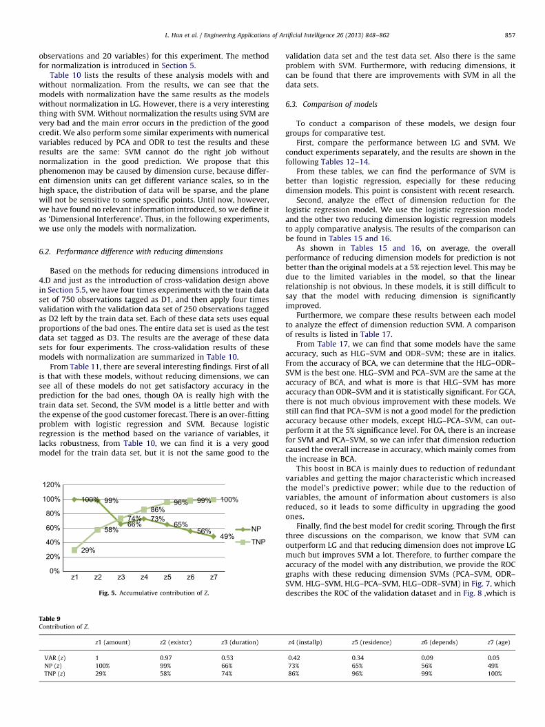
Calculate net information percentage NP¼SiVar(zi)/SiVar(xi) andtotal net information percentage TNP¼Ss

i ¼ 1Var zsð Þ=Sqj ¼ 1Var zj

� �,

the results listed in Table 9 and the original variables are labeled inbrackets. Fig. 5 shows the accumulative contribution of zi.

From Fig. 5, we can see z1,z2,z3 have 74% information of all, andhas 66% variance which is smaller than the sum of our zi. Thismeans by ODR we can only choose the orthogonal variablesz1,z2,z3 instead of the seven numerical attributes.

5.5. Cross-validation

As the best model is tailored to fit one sub-sample, the modeloften estimates the true error rate too optimistically. Therefore, toget a true estimate of the error rate, we applied two types ofcross-validation methodologies which were suggested by Zhanget al. (1999). First, as these typically did, the cross-validation

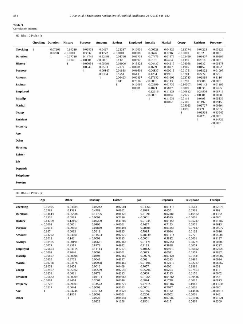
Table 3Correlation matrix.

H0: Rho¼0 Prob49r9

Checking Duration History Purpose Amount Savings Employed Installp Marital Coapp Resident Property

Checking 1 �0.07201 0.19219 0.02878 �0.0427 0.22287 0.10634 �0.00528 0.04326 �0.12774 �0.04223 �0.03226

0.0228 o0.0001 0.3632 0.1772 o0.0001 0.0008 0.8676 0.1716 o0.0001 0.182 0.3081

Duration 1 �0.07719 0.14749 0.62498 0.04766 0.05738 0.07475 0.01479 �0.02449 0.03407 0.30397

0.0146 o0.0001 o0.0001 0.132 0.0697 0.0181 0.6404 0.4392 0.2818 o0.0001

History 1 �0.09034 �0.05991 0.03906 0.13823 0.04437 0.04217 �0.04068 0.0632 �0.05378

0.0043 0.0583 0.2172 o0.0001 0.1609 0.1827 0.1987 0.0457 0.0892

Purpose 1 0.06847 �0.01868 0.01601 0.04837 0.00016 �0.01761 �0.03822 0.01097

0.0304 0.5551 0.613 0.1264 0.9961 0.5781 0.2272 0.7291

Amount 1 0.06463 �0.00837 �0.27132 �0.01609 �0.02783 0.02893 0.3116

0.041 0.7916 o0.0001 0.6113 0.3793 0.3608 o0.0001

Savings 1 0.12095 0.02199 0.01735 �0.10507 0.09142 0.01895

0.0001 0.4873 0.5837 0.0009 0.0038 0.5495

Employed 1 0.12616 0.11128 �0.00812 0.24508 0.08719

o0.0001 0.0004 0.7977 o0.0001 0.0058

Installp 1 0.11931 �0.0114 0.0493 0.05339

0.0002 0.7189 0.1192 0.0915

Marital 1 0.05063 �0.02727 �0.00694

0.1096 0.389 0.8265

Coapp 1 �0.02568 �0.15545

0.4173 o0.0001

Resident 1 0.14723

o0.0001

Property 1

Age

Other

Housing

Existcr

Job

Depends

Telephone

Foreign

H0: Rho¼0 Prob49r9

Age Other Housing Existcr Job Depends Telephone Foreign

Checking 0.05975 0.04684 0.02242 0.07601 0.04066 �0.01415 0.0663 �0.02676

0.0589 0.1388 0.4788 0.0162 0.1989 0.655 0.0361 0.398

Duration �0.03614 �0.05488 0.15705 �0.01128 0.21091 �0.02383 0.16472 �0.1382

0.2536 0.0828 o0.0001 0.7216 o0.0001 0.4515 o0.0001 o0.0001

History 0.14709 0.12197 0.06209 0.43707 0.01035 0.01155 0.05237 0.01387

o0.0001 0.0001 0.0496 o0.0001 0.7437 0.7153 0.0979 0.6613

Purpose 0.00131 �0.09661 0.01839 0.05494 0.00808 �0.03258 0.07837 �0.09972

0.967 0.0022 0.5613 0.0825 0.7985 0.3034 0.0132 0.0016

Amount 0.03272 �0.04601 0.13563 0.02079 0.28539 0.01714 0.277 �0.05005

0.3013 0.146 o0.0001 0.5113 o0.0001 0.5882 o0.0001 0.1137

Savings 0.08425 0.00191 0.00651 �0.02164 0.01171 0.02751 0.08721 0.00709

0.0077 0.9519 0.8372 0.4942 0.7115 0.3848 0.0058 0.8227

Employed 0.25623 �0.04015 0.11113 0.12579 0.10122 0.09719 0.06052 �0.02723

o0.0001 0.2046 0.0004 o0.0001 0.0013 0.0021 0.0557 0.3897

Installp 0.05827 �0.00098 0.0894 0.02167 0.09776 �0.07121 0.01441 �0.09002

0.0655 0.9752 0.0047 0.4937 0.002 0.0243 0.6489 0.0044

Marital 0.00778 �0.03676 0.09958 0.06467 �0.01196 0.12216 0.02727 0.06562

0.8058 0.2454 0.0016 0.0409 0.7057 0.0001 0.3889 0.038

Coapp �0.02987 �0.05902 �0.06589 �0.02545 �0.05796 0.0204 �0.07503 0.118

0.3453 0.0621 0.0372 0.4215 0.0669 0.5193 0.0176 0.0002

Resident 0.26642 0.00209 0.01194 0.08963 0.01265 0.04264 0.09536 �0.0541

o0.0001 0.9474 0.7061 0.0046 0.6894 0.1778 0.0025 0.0873

Property 0.07261 �0.09003 0.34522 �0.00777 0.27615 0.01187 0.1968 �0.13246

0.0217 0.0044 o0.0001 0.8063 o0.0001 0.7077 o0.0001 o0.0001

Age 1 �0.04235 0.30142 0.14925 0.01567 0.1182 0.14526 �0.00615

0.1809 o0.0001 o0.0001 0.6206 0.0002 o0.0001 0.846

Other 1 �0.0723 �0.04844 �0.00478 �0.07689 �0.01936 0.01521

0.0222 0.1258 0.8801 0.015 0.5409 0.6309


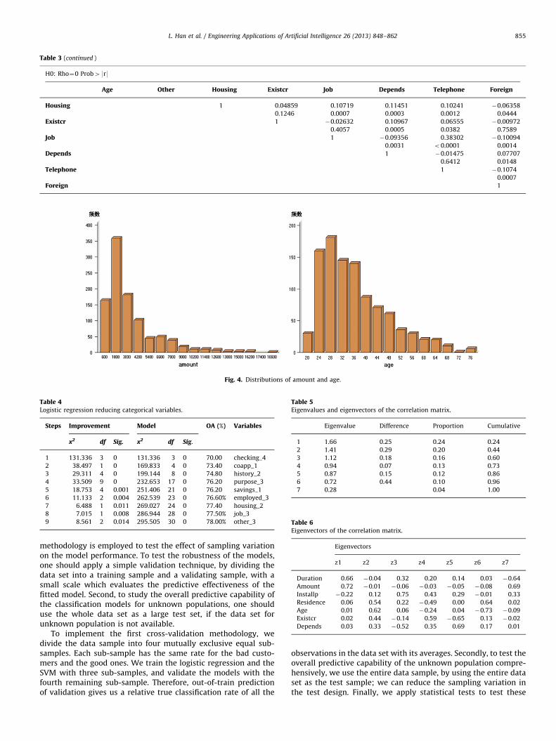
Table 3 (continued )

H0: Rho¼0 Prob49r9

Age Other Housing Existcr Job Depends Telephone Foreign

Housing 1 0.04859 0.10719 0.11451 0.10241 �0.06358

0.1246 0.0007 0.0003 0.0012 0.0444

Existcr 1 �0.02632 0.10967 0.06555 �0.00972

0.4057 0.0005 0.0382 0.7589

Job 1 �0.09356 0.38302 �0.10094

0.0031 o0.0001 0.0014

Depends 1 �0.01475 0.07707

0.6412 0.0148

Telephone 1 �0.1074

0.0007

Foreign 1

Fig. 4. Distributions of amount and age.

Table 4Logistic regression reducing categorical variables.

Steps Improvement Model OA (%) Variables

x2 df Sig. x2 df Sig.

1 131.336 3 0 131.336 3 0 70.00 checking_4

2 38.497 1 0 169.833 4 0 73.40 coapp_1

3 29.311 4 0 199.144 8 0 74.80 history_2

4 33.509 9 0 232.653 17 0 76.20 purpose_3

5 18.753 4 0.001 251.406 21 0 76.20 savings_1

6 11.133 2 0.004 262.539 23 0 76.60% employed_3

7 6.488 1 0.011 269.027 24 0 77.40 housing_2

8 7.015 1 0.008 286.944 28 0 77.50% job_3

9 8.561 2 0.014 295.505 30 0 78.00% other_3

Table 5Eigenvalues and eigenvectors of the correlation matrix.

Eigenvalue Difference Proportion Cumulative

1 1.66 0.25 0.24 0.24

2 1.41 0.29 0.20 0.44

3 1.12 0.18 0.16 0.60

4 0.94 0.07 0.13 0.73

5 0.87 0.15 0.12 0.86

6 0.72 0.44 0.10 0.96

7 0.28 0.04 1.00

Table 6Eigenvectors of the correlation matrix.

Eigenvectors

z1 z2 z3 z4 z5 z6 z7

Duration 0.66 �0.04 0.32 0.20 0.14 0.03 �0.64

Amount 0.72 �0.01 �0.06 �0.03 �0.05 �0.08 0.69

Installp �0.22 0.12 0.75 0.43 0.29 �0.01 0.33

Residence 0.06 0.54 0.22 �0.49 0.00 0.64 0.02

Age 0.01 0.62 0.06 �0.24 0.04 �0.73 �0.09

Existcr 0.02 0.44 �0.14 0.59 �0.65 0.13 �0.02

Depends 0.03 0.33 �0.52 0.35 0.69 0.17 0.01


methodology is employed to test the effect of sampling variationon the model performance. To test the robustness of the models,one should apply a simple validation technique, by dividing thedata set into a training sample and a validating sample, with asmall scale which evaluates the predictive effectiveness of thefitted model. Second, to study the overall predictive capability ofthe classification models for unknown populations, one shoulduse the whole data set as a large test set, if the data set forunknown population is not available.

To implement the first cross-validation methodology, wedivide the data sample into four mutually exclusive equal sub-samples. Each sub-sample has the same rate for the bad custo-mers and the good ones. We train the logistic regression and theSVM with three sub-samples, and validate the models with thefourth remaining sub-sample. Therefore, out-of-train predictionof validation gives us a relative true classification rate of all the

observations in the data set with its averages. Secondly, to test theoverall predictive capability of the unknown population compre-hensively, we use the entire data sample, by using the entire dataset as the test sample; we can reduce the sampling variation inthe test design. Finally, we apply statistical tests to test these

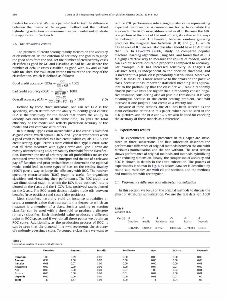
Table 8Variance of Z.

Var (z) z1

Duration

z3

Installp

z4

Residence

z5

Age

z6

Existcr

z7

Depends

0.587915 0.401513 0.7569 0.000126 0.971213 0.8464


models for accuracy. We use a paired-t test to test the differencebetween the means of the original method and the methodhybridizing reduction of dimension in experimental and illustratethe application in Section 6.

5.6. The evaluation criteria

The problem of credit scoring mainly focuses on the accuracyof classification. As the criterion of accuracy, the goal is to judgethe good ones from the bad. Let the number of creditworthy casesclassified as good be GG and classified as bad be GB; denote thenumber of default cases classified as good with BG and as badwith BB. Then, the evaluation criteria measure the accuracy of theclassification, which is defined as follows:

Good credit accuracy GCAð Þ ¼GG

GGþGB� 100%

Bad credit accuracy BCAð Þ ¼BB

BGþBB� 100%

Overall accuracy OAð Þ ¼GGþBB

GGþGBþBGþBB� 100% ð15Þ

Defined by these three indicators, one can see GCA is thespecificity, which determines the ability to identify good clients;BCA is the sensitivity for the model that shows the ability toidentify bad customers. At the same time, OA gives the totalefficiency of the model and reflects prediction accuracy of themodel and can compare with others.

In our study, Type I error occurs when a bad credit is classifiedas good credit, which equals 1-BCA. And Type II error occurs whena good credit is classified as a bad credit, which equals 1-GCA. Forcredit scoring, Type I error is more critical than Type II error. Notethat all these measures with Type I error and Type II error aremostly obtained using a 0.5 probability threshold for the classifica-tion. However, the use of arbitrary cut-off probabilities makes thecomputed error rates difficult to interpret and the use of a relevantpay-off function and prior probabilities to determine the optionalmodel could lead to some types of bias on the results. Bradley(1997) gave a way to judge the efficiency with ROC. The receiveroperating characteristics (ROC) graph is useful for organizingclassifiers and visualizing their performance. The ROC graph is atwo-dimensional graph in which the BCA (true positives) rate isplotted on the Y axis and the 1-GCA (false positives) rate is plottedon the X axis. The ROC graph depicts relative trade-offs betweenbenefits (true positives) and costs (false positives).

Most classifiers naturally yield an instance probability orscore, a numeric value that represents the degree to which aninstance is a member of a class. Such a ranking or scoringclassifier can be used with a threshold to produce a discrete(binary) classifier. Each threshold value produces a differentpoint in ROC space, and if we join all these points we obtain anROC curve. Additionally, as the production process of ROC, itcan be seen that the diagonal line y¼x represents the strategyof randomly guessing a class. To compare classifiers we want to

Table 7Correlation matrix of numerical attributes.

Duration Amount Installp

Duration 1.00 0.39 0.01

Amount 0.39 1.00 0.07

Installp 0.01 0.07 1.00

Residence 0.00 0.00 0.00

Age 0.00 0.00 0.00

Existcr 0.00 0.00 0.00

Depends 0.00 0.00 0.01

Total 1.40 1.47 1.09

reduce ROC performance into a single scalar value representingexpected performance. A common method is to calculate thearea under the ROC curve, abbreviated as AUC. Because the AUCis a portion of the area of the unit square, its value will alwaysbe between 0 and 1. However, because random guessingproduces the diagonal line between (0, 0) and (1, 1), whichhas an area of 0.5, no realistic classifier should have an AUC lessthan 0.5. In Fawcett’s (2006) study, he compared popularmachine learning algorithms using AUC and found that AUC isa highly effective way to measure the results of models, and itcan exhibit several desirable properties compared to accuracy.For example, AUC has increased sensitivity in analysis ofvariance tests, is independent to the decision threshold, andis invariant to a priori class probability distributions. Moreover,the AUC measure is more sensitive to the errors on the positiveclass, because it has important statistical meaning: it is equiva-lent to the probability that the classifier will rank a randomlychosen positive instance higher than a randomly chosen nega-tive instance, considering also all possible thresholds. It is verymeaningful because in the credit scoring problem, cost willincrease if one judges a bad credit as a worthy one.

Because of these reasons, the AUC has been selected as themain evaluation criteria in this paper, which can be seen in theROC pictures, and the BCA and GCA are also be used for checkingthe accuracy of these models as a reference.

6. Experiments results

The experimental results presented in this paper are struc-tured in three subsections. The first subsection describes theperformance difference of original methods between the one withattributes normalization and the one without. The next sectionshows performance of original methods and methods hybridizingwith reducing dimension. Finally, the comparison of accuracy andROC is shown in details in the third subsection. The process ofexperiments is shown in Fig. 6 as below, data set is described byround said, variables are with elliptic sections, and the methodsand models are with rectangular.

6.1. Performance difference with attributes normalization

In this section, we focus on the original methods to discuss theeffect of attributes normalization. We use the test data set (1000

Residence Age Existcr Depends

0.00 0.00 0.00 0.00

0.00 0.00 0.00 0.00

0.00 0.00 0.00 0.01

1.00 0.07 0.01 0.00

0.07 1.00 0.02 0.01

0.01 0.02 1.00 0.01

0.00 0.01 0.01 1.00

1.09 1.11 1.04 1.03


observations and 20 variables) for this experiment. The methodfor normalization is introduced in Section 5.

Table 10 lists the results of these analysis models with andwithout normalization. From the results, we can see that themodels with normalization have the same results as the modelswithout normalization in LG. However, there is a very interestingthing with SVM. Without normalization the results using SVM arevery bad and the main error occurs in the prediction of the goodcredit. We also perform some similar experiments with numericalvariables reduced by PCA and ODR to test the results and theseresults are the same: SVM cannot do the right job withoutnormalization in the good prediction. We propose that thisphenomenon may be caused by dimension curse, because differ-ent dimension units can get different variance scales, so in thehigh space, the distribution of data will be sparse, and the planewill not be sensitive to some specific points. Until now, however,we have found no relevant information introduced, so we define itas ‘Dimensional Interference’. Thus, in the following experiments,we use only the models with normalization.

6.2. Performance difference with reducing dimensions

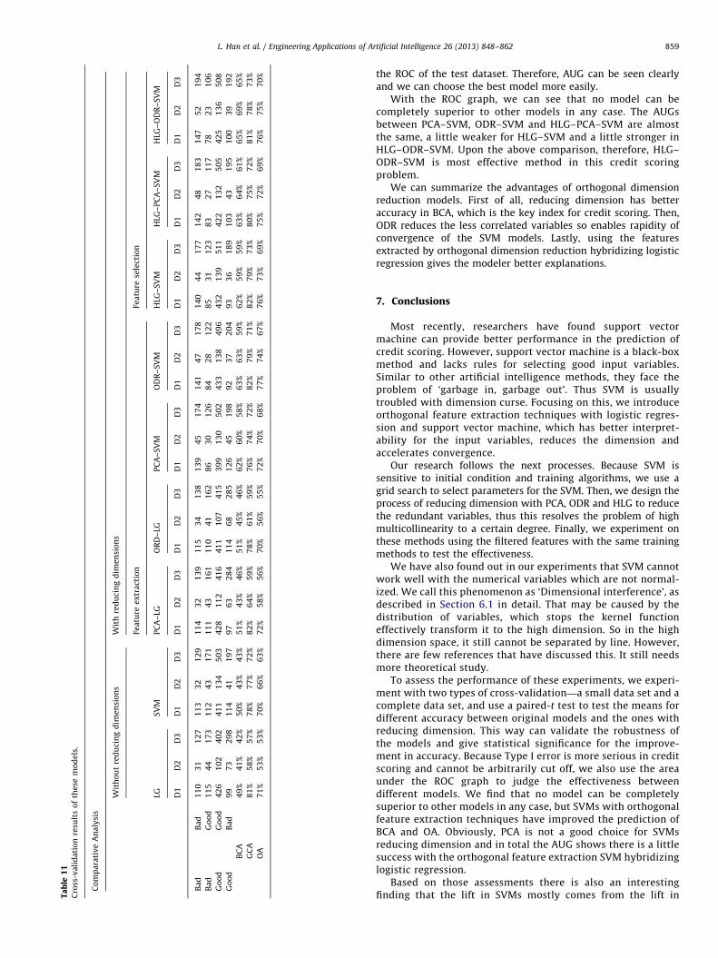
Based on the methods for reducing dimensions introduced in4.D and just as the introduction of cross-validation design abovein Section 5.5, we have four times experiments with the train dataset of 750 observations tagged as D1, and then apply four timesvalidation with the validation data set of 250 observations taggedas D2 left by the train data set. Each of these data sets uses equalproportions of the bad ones. The entire data set is used as the testdata set tagged as D3. The results are the average of these datasets for four experiments. The cross-validation results of thesemodels with normalization are summarized in Table 10.

From Table 11, there are several interesting findings. First of allis that with these models, without reducing dimensions, we cansee all of these models do not get satisfactory accuracy in theprediction for the bad ones, though OA is really high with thetrain data set. Second, the SVM model is a little better and withthe expense of the good customer forecast. There is an over-fittingproblem with logistic regression and SVM. Because logisticregression is the method based on the variance of variables, itlacks robustness, from Table 10, we can find it is a very goodmodel for the train data set, but it is not the same good to the

Table 9Contribution of Z.

z1 (amount) z2 (existcr) z3 (duration)

VAR (z) 1 0.97 0.53

NP (z) 100% 99% 66%

TNP (z) 29% 58% 74%

100% 99%

66%73%

65%56%

49%

29%

58%74%

86%96% 99% 100%

0%

20%

40%

60%

80%

100%

120%

z1 z2 z3 z4 z5 z6 z7

NP

TNP

Fig. 5. Accumulative contribution of Z.

validation data set and the test data set. Also there is the sameproblem with SVM. Furthermore, with reducing dimensions, itcan be found that there are improvements with SVM in all thedata sets.

6.3. Comparison of models

To conduct a comparison of these models, we design fourgroups for comparative test.

First, compare the performance between LG and SVM. Weconduct experiments separately, and the results are shown in thefollowing Tables 12–14.

From these tables, we can find the performance of SVM isbetter than logistic regression, especially for these reducingdimension models. This point is consistent with recent research.

Second, analyze the effect of dimension reduction for thelogistic regression model. We use the logistic regression modeland the other two reducing dimension logistic regression modelsto apply comparative analysis. The results of the comparison canbe found in Tables 15 and 16.

As shown in Tables 15 and 16, on average, the overallperformance of reducing dimension models for prediction is notbetter than the original models at a 5% rejection level. This may bedue to the limited variables in the model, so that the linearrelationship is not obvious. In these models, it is still difficult tosay that the model with reducing dimension is significantlyimproved.

Furthermore, we compare these results between each modelto analyze the effect of dimension reduction SVM. A comparisonof results is listed in Table 17.

From Table 17, we can find that some models have the sameaccuracy, such as HLG–SVM and ODR–SVM; these are in italics.From the accuracy of BCA, we can determine that the HLG–ODR–SVM is the best one. HLG–SVM and PCA–SVM are the same at theaccuracy of BCA, and what is more is that HLG–SVM has moreaccuracy than ODR–SVM and it is statistically significant. For GCA,there is not much obvious improvement with these models. Westill can find that PCA–SVM is not a good model for the predictionaccuracy because other models, except HLG–PCA–SVM, can out-perform it at the 5% significance level. For OA, there is an increasefor SVM and PCA–SVM, so we can infer that dimension reductioncaused the overall increase in accuracy, which mainly comes fromthe increase in BCA.

This boost in BCA is mainly dues to reduction of redundantvariables and getting the major characteristic which increasedthe model’s predictive power; while due to the reduction ofvariables, the amount of information about customers is alsoreduced, so it leads to some difficulty in upgrading the goodones.

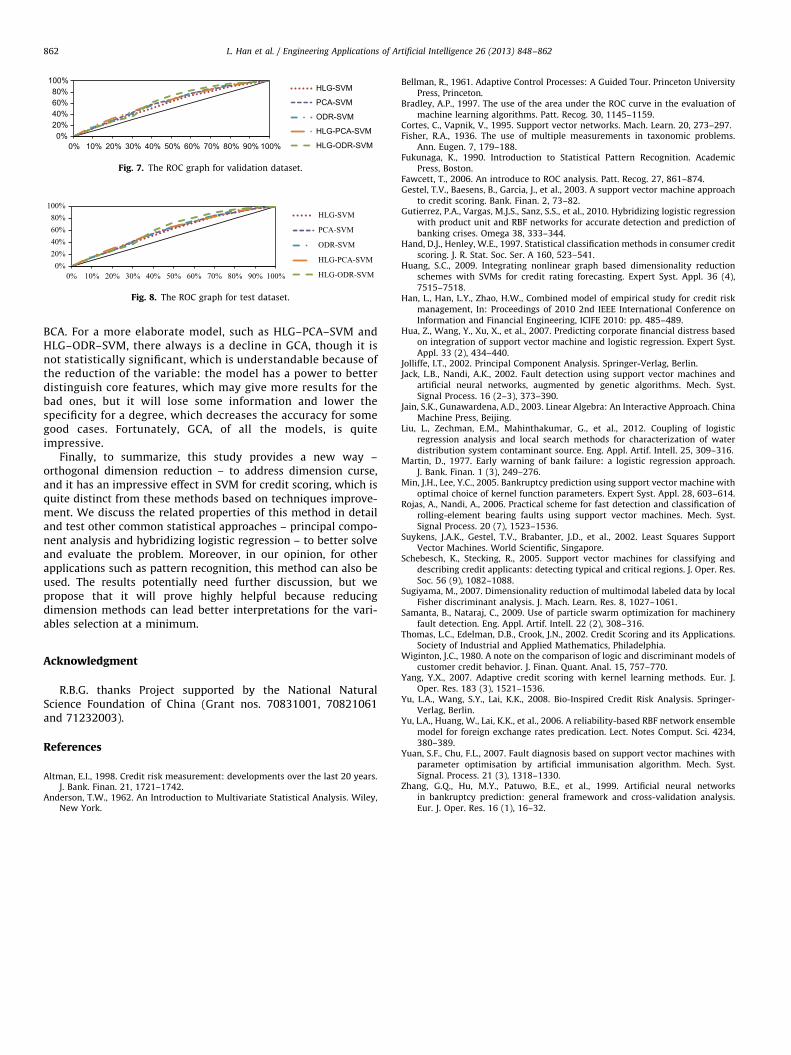
Finally, find the best model for credit scoring. Through the firstthree discussions on the comparison, we know that SVM canoutperform LG and that reducing dimension does not improve LGmuch but improves SVM a lot. Therefore, to further compare theaccuracy of the model with any distribution, we provide the ROCgraphs with these reducing dimension SVMs (PCA–SVM, ODR–SVM, HLG–SVM, HLG–PCA–SVM, HLG–ODR–SVM) in Fig. 7, whichdescribes the ROC of the validation dataset and in Fig. 8 ,which is

z4 (installp) z5 (residence) z6 (depends) z7 (age)

0.42 0.34 0.09 0.05

73% 65% 56% 49%

86% 96% 99% 100%

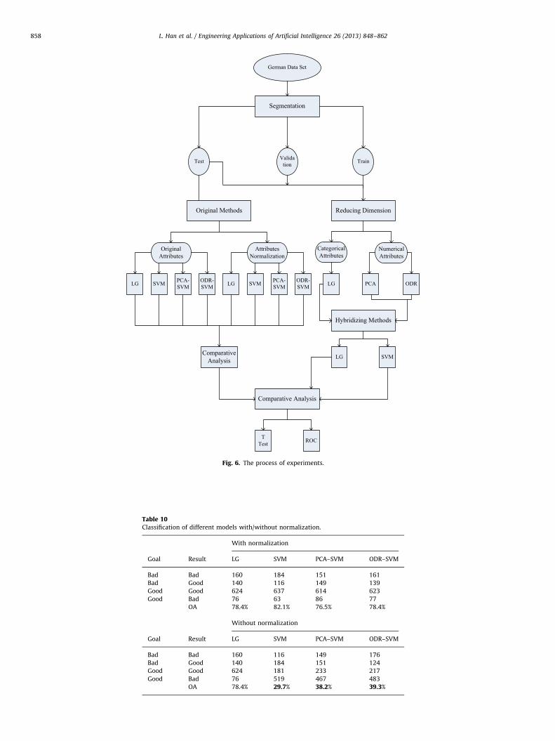
Table 10Classification of different models with/without normalization.

With normalization

Goal Result LG SVM PCA–SVM ODR–SVM

Bad Bad 160 184 151 161

Bad Good 140 116 149 139

Good Good 624 637 614 623

Good Bad 76 63 86 77

OA 78.4% 82.1% 76.5% 78.4%

Without normalization

Goal Result LG SVM PCA–SVM ODR–SVM

Bad Bad 160 116 149 176

Bad Good 140 184 151 124

Good Good 624 181 233 217

Good Bad 76 519 467 483

OA 78.4% 29.7% 38.2% 39.3%

Segmentation

Original Methods Reducing Dimension

German Data Set

Test Validation Train

LG PCALGPCA-SVM ODR

CategoricalAttributes

NumericalAttributes

Comparative Analysis

Hybridizing Methods

LG SVM

TTest ROC

AttributesNormalization

ComparativeAnalysis

SVM ODR-SVMLG PCA-

SVMSVM ODR-SVM

OriginalAttributes

Fig. 6. The process of experiments.


Ta

ble

11

Cro

ss-v

ali

da

tio

nre

sult

so

fth

ese

mo

de

ls.

Co

mp

ara

tiv

eA

na

lysi

s

Wit

ho

ut

red

uci

ng

dim

en

sio

ns

Wit

hre

du

cin

gd

ime

nsi

on

s

Fea

ture

ex

tra

ctio

nFe

atu

rese

lect

ion

LGS

VM

PC

A–

LGO

RD

–LG

PC

A–

SV

MO

DR

–S

VM

HLG

–S

VM

HLG

–P

CA

–S

VM

HLG

–O

DR

–S

VM

D1

D2

D3

D1

D2

D3

D1

D2

D3

D1

D2

D3

D1

D2

D3

D1

D2

D3

D1

D2

D3

D1

D2

D3

D1

D2

D3

Ba

dB

ad

11

03

11

27

11

33

21

29

11

43

21

39

11

53

41

38

13

94

51

74

14

14

71

78

14

04

41

77

14

24

81

83

14

75

21

94

Ba

dG

oo

d1

15

44

17

31

12

43

17

11

11

43

16

11

10

41

16

28

63

01

26

84

28

12

28

53

11

23

83

27

11

77

82

31

06

Go

od

Go

od

42

61

02

40

24

11

13

45

03

42

81

12

41

64

11

10

74

15

39

91

30

50

24

33

13

84

96

43

21

39

51

14

22

13

25

05

42

51

36

50

8

Go

od

Ba

d9

97

32

98

11

44

11

97

97

63

28

41

14

68

28

51

26

45

19

89

23

72

04

93

36

18

91

03

43

19

51

00

39

19

2

BC

A4

9%

41

%4

2%

50

%4

3%

43

%5

1%

43

%4

6%

51

%4

5%

46

%6

2%

60

%5

8%

63

%6

3%

59

%6

2%

59

%5

9%

63

%6

4%

61

%6

5%

69

%6

5%

GC

A8

1%

58

%5

7%

78

%7

7%

72

%8

2%

64

%5

9%

78

%6

1%

59

%7

6%

74

%7

2%

82

%7

9%

71

%8

2%

79

%7

3%

80

%7

5%

72

%8

1%

78

%7

3%

OA

71

%5

3%

53

%7

0%

66

%6

3%

72

%5

8%

56

%7

0%

56

%5

5%

72

%7

0%

68

%7

7%

74

%6

7%

76

%7

3%

69

%7

5%

72

%6

9%

76

%7

5%

70

%


the ROC of the test dataset. Therefore, AUG can be seen clearlyand we can choose the best model more easily.

With the ROC graph, we can see that no model can becompletely superior to other models in any case. The AUGsbetween PCA–SVM, ODR–SVM and HLG–PCA–SVM are almostthe same, a little weaker for HLG–SVM and a little stronger inHLG–ODR–SVM. Upon the above comparison, therefore, HLG–ODR–SVM is most effective method in this credit scoringproblem.

We can summarize the advantages of orthogonal dimensionreduction models. First of all, reducing dimension has betteraccuracy in BCA, which is the key index for credit scoring. Then,ODR reduces the less correlated variables so enables rapidity ofconvergence of the SVM models. Lastly, using the featuresextracted by orthogonal dimension reduction hybridizing logisticregression gives the modeler better explanations.

7. Conclusions

Most recently, researchers have found support vectormachine can provide better performance in the prediction ofcredit scoring. However, support vector machine is a black-boxmethod and lacks rules for selecting good input variables.Similar to other artificial intelligence methods, they face theproblem of ‘garbage in, garbage out’. Thus SVM is usuallytroubled with dimension curse. Focusing on this, we introduceorthogonal feature extraction techniques with logistic regres-sion and support vector machine, which has better interpret-ability for the input variables, reduces the dimension andaccelerates convergence.

Our research follows the next processes. Because SVM issensitive to initial condition and training algorithms, we use agrid search to select parameters for the SVM. Then, we design theprocess of reducing dimension with PCA, ODR and HLG to reducethe redundant variables, thus this resolves the problem of highmulticollinearity to a certain degree. Finally, we experiment onthese methods using the filtered features with the same trainingmethods to test the effectiveness.

We have also found out in our experiments that SVM cannotwork well with the numerical variables which are not normal-ized. We call this phenomenon as ‘Dimensional interference’, asdescribed in Section 6.1 in detail. That may be caused by thedistribution of variables, which stops the kernel functioneffectively transform it to the high dimension. So in the highdimension space, it still cannot be separated by line. However,there are few references that have discussed this. It still needsmore theoretical study.

To assess the performance of these experiments, we experi-ment with two types of cross-validation—a small data set and acomplete data set, and use a paired-t test to test the means fordifferent accuracy between original models and the ones withreducing dimension. This way can validate the robustness ofthe models and give statistical significance for the improve-ment in accuracy. Because Type I error is more serious in creditscoring and cannot be arbitrarily cut off, we also use the areaunder the ROC graph to judge the effectiveness betweendifferent models. We find that no model can be completelysuperior to other models in any case, but SVMs with orthogonalfeature extraction techniques have improved the prediction ofBCA and OA. Obviously, PCA is not a good choice for SVMsreducing dimension and in total the AUG shows there is a littlesuccess with the orthogonal feature extraction SVM hybridizinglogistic regression.

Based on those assessments there is also an interestingfinding that the lift in SVMs mostly comes from the lift in

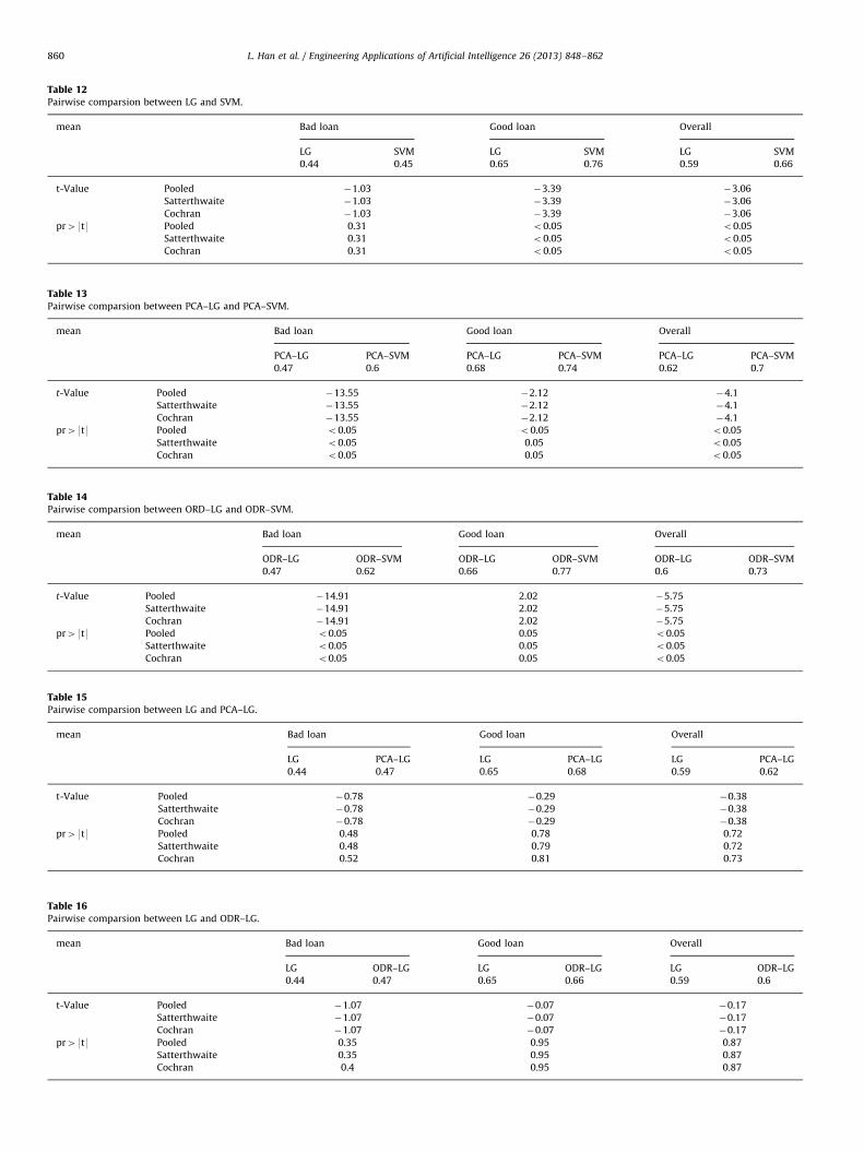
Table 16Pairwise comparsion between LG and ODR–LG.

mean Bad loan Good loan Overall

LG ODR–LG LG ODR–LG LG ODR–LG

0.44 0.47 0.65 0.66 0.59 0.6

t-Value Pooled �1.07 �0.07 �0.17

Satterthwaite �1.07 �0.07 �0.17

Cochran �1.07 �0.07 �0.17

pr49t9 Pooled 0.35 0.95 0.87

Satterthwaite 0.35 0.95 0.87

Cochran 0.4 0.95 0.87

Table 15Pairwise comparsion between LG and PCA–LG.


LG PCA–LG LG PCA–LG LG PCA–LG

0.44 0.47 0.65 0.68 0.59 0.62

t-Value Pooled �0.78 �0.29 �0.38


Cochran �0.78 �0.29 �0.38

pr49t9 Pooled 0.48 0.78 0.72

Satterthwaite 0.48 0.79 0.72

Cochran 0.52 0.81 0.73

Table 12Pairwise comparsion between LG and SVM.


LG SVM LG SVM LG SVM

0.44 0.45 0.65 0.76 0.59 0.66

t-Value Pooled �1.03 �3.39 �3.06


Cochran �1.03 �3.39 �3.06

pr49t9 Pooled 0.31 o0.05 o0.05

Satterthwaite 0.31 o0.05 o0.05

Cochran 0.31 o0.05 o0.05

Table 13Pairwise comparsion between PCA–LG and PCA–SVM.


PCA–LG PCA–SVM PCA–LG PCA–SVM PCA–LG PCA–SVM

0.47 0.6 0.68 0.74 0.62 0.7

t-Value Pooled �13.55 �2.12 �4.1


Cochran �13.55 �2.12 �4.1

pr49t9 Pooled o0.05 o0.05 o0.05

Satterthwaite o0.05 0.05 o0.05

Cochran o0.05 0.05 o0.05

Table 14Pairwise comparsion between ORD–LG and ODR–SVM.


ODR–LG ODR–SVM ODR–LG ODR–SVM ODR–LG ODR–SVM

0.47 0.62 0.66 0.77 0.6 0.73

t-Value Pooled �14.91 2.02 �5.75

Satterthwaite �14.91 2.02 �5.75

Cochran �14.91 2.02 �5.75

pr49t9 Pooled o0.05 0.05 o0.05

Satterthwaite o0.05 0.05 o0.05

Cochran o0.05 0.05 o0.05


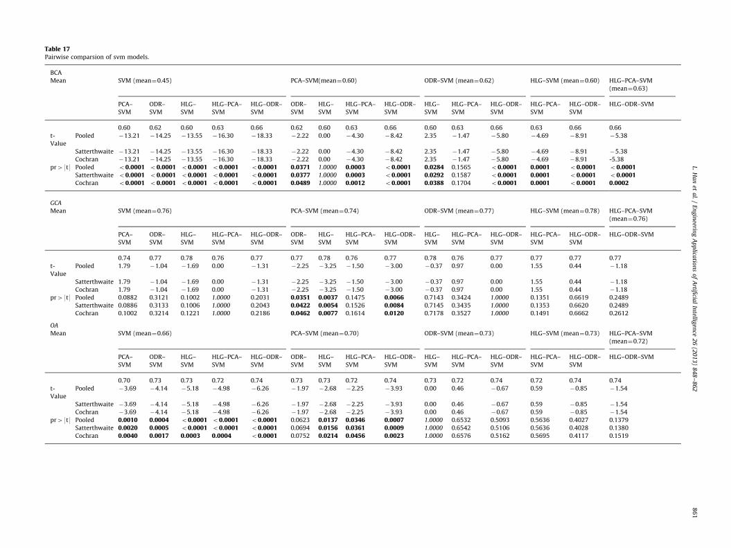
Table 17Pairwise comparsion of svm models.

BCA

Mean SVM (mean¼0.45) PCA–SVM(mean¼0.60) ODR–SVM (mean¼0.62) HLG–SVM (mean¼0.60) HLG–PCA–SVM

(mean¼0.63)

PCA–

SVM

ODR–

SVM

HLG–

SVM

HLG–PCA–

SVM

HLG–ODR–

SVM

ODR–

SVM

HLG–

SVM

HLG–PCA–

SVM

HLG–ODR–

SVM

HLG–

SVM

HLG–PCA–

SVM

HLG–ODR–

SVM

HLG–PCA–

SVM

HLG–ODR–

SVM

HLG–ODR–SVM

0.60 0.62 0.60 0.63 0.66 0.62 0.60 0.63 0.66 0.60 0.63 0.66 0.63 0.66 0.66

t-

Value

Pooled �13.21 �14.25 �13.55 �16.30 �18.33 �2.22 0.00 �4.30 �8.42 2.35 �1.47 �5.80 �4.69 �8.91 �5.38

Satterthwaite �13.21 �14.25 �13.55 �16.30 �18.33 �2.22 0.00 �4.30 �8.42 2.35 �1.47 �5.80 �4.69 �8.91 �5.38

Cochran �13.21 �14.25 �13.55 �16.30 �18.33 �2.22 0.00 �4.30 �8.42 2.35 �1.47 �5.80 �4.69 �8.91 -5.38

pr49t9 Pooled o0.0001 o0.0001 o0.0001 o0.0001 o0.0001 0.0371 1.0000 0.0003 o0.0001 0.0284 0.1565 o0.0001 0.0001 o0.0001 o0.0001Satterthwaite o0.0001 o0.0001 o0.0001 o0.0001 o0.0001 0.0377 1.0000 0.0003 o0.0001 0.0292 0.1587 o0.0001 0.0001 o0.0001 o0.0001Cochran o0.0001 o0.0001 o0.0001 o0.0001 o0.0001 0.0489 1.0000 0.0012 o0.0001 0.0388 0.1704 o0.0001 0.0001 o0.0001 0.0002

GCA

Mean SVM (mean¼0.76) PCA–SVM (mean¼0.74) ODR–SVM (mean¼0.77) HLG–SVM (mean¼0.78) HLG–PCA–SVM

(mean¼0.76)

PCA–

SVM

ODR–

SVM

HLG–

SVM

HLG–PCA–

SVM

HLG–ODR–

SVM

ODR–

SVM

HLG–

SVM

HLG–PCA–

SVM

HLG–ODR–

SVM

HLG–

SVM

HLG–PCA–

SVM

HLG–ODR–

SVM

HLG–PCA–

SVM

HLG–ODR–

SVM

HLG–ODR–SVM

0.74 0.77 0.78 0.76 0.77 0.77 0.78 0.76 0.77 0.78 0.76 0.77 0.77 0.77 0.77

t-

Value

Pooled 1.79 �1.04 �1.69 0.00 �1.31 �2.25 �3.25 �1.50 �3.00 �0.37 0.97 0.00 1.55 0.44 �1.18

Satterthwaite 1.79 �1.04 �1.69 0.00 �1.31 �2.25 �3.25 �1.50 �3.00 �0.37 0.97 0.00 1.55 0.44 �1.18

Cochran 1.79 �1.04 �1.69 0.00 �1.31 �2.25 �3.25 �1.50 �3.00 �0.37 0.97 0.00 1.55 0.44 �1.18

pr49t9 Pooled 0.0882 0.3121 0.1002 1.0000 0.2031 0.0351 0.0037 0.1475 0.0066 0.7143 0.3424 1.0000 0.1351 0.6619 0.2489

Satterthwaite 0.0886 0.3133 0.1006 1.0000 0.2043 0.0422 0.0054 0.1526 0.0084 0.7145 0.3435 1.0000 0.1353 0.6620 0.2489

Cochran 0.1002 0.3214 0.1221 1.0000 0.2186 0.0462 0.0077 0.1614 0.0120 0.7178 0.3527 1.0000 0.1491 0.6662 0.2612

OA

Mean SVM (mean¼0.66) PCA–SVM (mean¼0.70) ODR–SVM (mean¼0.73) HLG–SVM (mean¼0.73) HLG–PCA–SVM

(mean¼0.72)

PCA–

SVM

ODR–

SVM

HLG–

SVM

HLG–PCA–

SVM

HLG–ODR–

SVM

ODR–

SVM

HLG–

SVM

HLG–PCA–

SVM

HLG–ODR–

SVM

HLG–

SVM

HLG–PCA–

SVM

HLG–ODR–

SVM

HLG–PCA–

SVM

HLG–ODR–

SVM

HLG–ODR–SVM

0.70 0.73 0.73 0.72 0.74 0.73 0.73 0.72 0.74 0.73 0.72 0.74 0.72 0.74 0.74

t-

Value

Pooled �3.69 �4.14 �5.18 �4.98 �6.26 �1.97 �2.68 �2.25 �3.93 0.00 0.46 �0.67 0.59 �0.85 �1.54

Satterthwaite �3.69 �4.14 �5.18 �4.98 �6.26 �1.97 �2.68 �2.25 �3.93 0.00 0.46 �0.67 0.59 �0.85 �1.54

Cochran �3.69 �4.14 �5.18 �4.98 �6.26 �1.97 �2.68 �2.25 �3.93 0.00 0.46 �0.67 0.59 �0.85 �1.54

pr49t9 Pooled 0.0010 0.0004 o0.0001 o0.0001 o0.0001 0.0623 0.0137 0.0346 0.0007 1.0000 0.6532 0.5093 0.5636 0.4027 0.1379

Satterthwaite 0.0020 0.0005 o0.0001 o0.0001 o0.0001 0.0694 0.0156 0.0361 0.0009 1.0000 0.6542 0.5106 0.5636 0.4028 0.1380

Cochran 0.0040 0.0017 0.0003 0.0004 o0.0001 0.0752 0.0214 0.0456 0.0023 1.0000 0.6576 0.5162 0.5695 0.4117 0.1519

L.H

an

eta

l./

En

gin

eering

Ap

plica

tion

so

fA

rtificia

lIn

telligen

ce2

6(2

01

3)

84

8–

86

28

61

0%20%40%60%80%

100%

0% 10% 20% 30% 40% 50% 60% 70% 80% 90% 100%

HLG-SVM

PCA-SVM

ODR-SVM

HLG-PCA-SVM

HLG-ODR-SVM

Fig. 8. The ROC graph for test dataset.

0%20%40%60%80%

100%

0% 10% 20% 30% 40% 50% 60% 70% 80% 90% 100%

HLG-SVM

PCA-SVM

ODR-SVM

HLG-PCA-SVM

HLG-ODR-SVM

Fig. 7. The ROC graph for validation dataset.


BCA. For a more elaborate model, such as HLG–PCA–SVM andHLG–ODR–SVM, there always is a decline in GCA, though it isnot statistically significant, which is understandable because ofthe reduction of the variable: the model has a power to betterdistinguish core features, which may give more results for thebad ones, but it will lose some information and lower thespecificity for a degree, which decreases the accuracy for somegood cases. Fortunately, GCA, of all the models, is quiteimpressive.

Finally, to summarize, this study provides a new way –orthogonal dimension reduction – to address dimension curse,and it has an impressive effect in SVM for credit scoring, which isquite distinct from these methods based on techniques improve-ment. We discuss the related properties of this method in detailand test other common statistical approaches – principal compo-nent analysis and hybridizing logistic regression – to better solveand evaluate the problem. Moreover, in our opinion, for otherapplications such as pattern recognition, this method can also beused. The results potentially need further discussion, but wepropose that it will prove highly helpful because reducingdimension methods can lead better interpretations for the vari-ables selection at a minimum.

Acknowledgment

R.B.G. thanks Project supported by the National NaturalScience Foundation of China (Grant nos. 70831001, 70821061and 71232003).

References

Altman, E.I., 1998. Credit risk measurement: developments over the last 20 years.J. Bank. Finan. 21, 1721–1742.

Anderson, T.W., 1962. An Introduction to Multivariate Statistical Analysis. Wiley,New York.

Bellman, R., 1961. Adaptive Control Processes: A Guided Tour. Princeton UniversityPress, Princeton.

Bradley, A.P., 1997. The use of the area under the ROC curve in the evaluation ofmachine learning algorithms. Patt. Recog. 30, 1145–1159.

Cortes, C., Vapnik, V., 1995. Support vector networks. Mach. Learn. 20, 273–297.Fisher, R.A., 1936. The use of multiple measurements in taxonomic problems.

Ann. Eugen. 7, 179–188.Fukunaga, K., 1990. Introduction to Statistical Pattern Recognition. Academic

Press, Boston.Fawcett, T., 2006. An introduce to ROC analysis. Patt. Recog. 27, 861–874.Gestel, T.V., Baesens, B., Garcia, J., et al., 2003. A support vector machine approach

to credit scoring. Bank. Finan. 2, 73–82.Gutierrez, P.A., Vargas, M.J.S., Sanz, S.S., et al., 2010. Hybridizing logistic regression

with product unit and RBF networks for accurate detection and prediction ofbanking crises. Omega 38, 333–344.

Hand, D.J., Henley, W.E., 1997. Statistical classification methods in consumer creditscoring. J. R. Stat. Soc. Ser. A 160, 523–541.

Huang, S.C., 2009. Integrating nonlinear graph based dimensionality reductionschemes with SVMs for credit rating forecasting. Expert Syst. Appl. 36 (4),7515–7518.

Han, L., Han, L.Y., Zhao, H.W., Combined model of empirical study for credit riskmanagement, In: Proceedings of 2010 2nd IEEE International Conference onInformation and Financial Engineering, ICIFE 2010: pp. 485–489.

Hua, Z., Wang, Y., Xu, X., et al., 2007. Predicting corporate financial distress basedon integration of support vector machine and logistic regression. Expert Syst.Appl. 33 (2), 434–440.

Jolliffe, I.T., 2002. Principal Component Analysis. Springer-Verlag, Berlin.Jack, L.B., Nandi, A.K., 2002. Fault detection using support vector machines and

artificial neural networks, augmented by genetic algorithms. Mech. Syst.Signal Process. 16 (2–3), 373–390.

Jain, S.K., Gunawardena, A.D., 2003. Linear Algebra: An Interactive Approach. ChinaMachine Press, Beijing.

Liu, L., Zechman, E.M., Mahinthakumar, G., et al., 2012. Coupling of logisticregression analysis and local search methods for characterization of waterdistribution system contaminant source. Eng. Appl. Artif. Intell. 25, 309–316.

Martin, D., 1977. Early warning of bank failure: a logistic regression approach.J. Bank. Finan. 1 (3), 249–276.

Min, J.H., Lee, Y.C., 2005. Bankruptcy prediction using support vector machine withoptimal choice of kernel function parameters. Expert Syst. Appl. 28, 603–614.

Rojas, A., Nandi, A., 2006. Practical scheme for fast detection and classification ofrolling-element bearing faults using support vector machines. Mech. Syst.Signal Process. 20 (7), 1523–1536.

Suykens, J.A.K., Gestel, T.V., Brabanter, J.D., et al., 2002. Least Squares SupportVector Machines. World Scientific, Singapore.

Schebesch, K., Stecking, R., 2005. Support vector machines for classifying anddescribing credit applicants: detecting typical and critical regions. J. Oper. Res.Soc. 56 (9), 1082–1088.

Sugiyama, M., 2007. Dimensionality reduction of multimodal labeled data by localFisher discriminant analysis. J. Mach. Learn. Res. 8, 1027–1061.

Samanta, B., Nataraj, C., 2009. Use of particle swarm optimization for machineryfault detection. Eng. Appl. Artif. Intell. 22 (2), 308–316.

Thomas, L.C., Edelman, D.B., Crook, J.N., 2002. Credit Scoring and its Applications.Society of Industrial and Applied Mathematics, Philadelphia.

Wiginton, J.C., 1980. A note on the comparison of logic and discriminant models ofcustomer credit behavior. J. Finan. Quant. Anal. 15, 757–770.

Yang, Y.X., 2007. Adaptive credit scoring with kernel learning methods. Eur. J.Oper. Res. 183 (3), 1521–1536.

Yu, L.A., Wang, S.Y., Lai, K.K., 2008. Bio-Inspired Credit Risk Analysis. Springer-Verlag, Berlin.

Yu, L.A., Huang, W., Lai, K.K., et al., 2006. A reliability-based RBF network ensemblemodel for foreign exchange rates predication. Lect. Notes Comput. Sci. 4234,380–389.

Yuan, S.F., Chu, F.L., 2007. Fault diagnosis based on support vector machines withparameter optimisation by artificial immunisation algorithm. Mech. Syst.Signal. Process. 21 (3), 1318–1330.

Zhang, G.Q., Hu, M.Y., Patuwo, B.E., et al., 1999. Artificial neural networksin bankruptcy prediction: general framework and cross-validation analysis.Eur. J. Oper. Res. 16 (1), 16–32.

orthogonal support vector machine for credit scoring · the most commonly used techniques for...

Documents