orthorhombic anisotropy : a physical seismic modeling … · 1 orthorhombic anisotropy: a physical...

1

Orthorhombic anisotropy: A physical seismic modeling studyScott P. Cheadle∗, R. James Brown‡ , and Don C. Lawton‡

Presented at the 60th Annual International Meeting, Society of Exploration Geophysicists. Manuscript received by the Editor August 24,1990; revised manuscript received March 21, 1991.

∗ Formerly Department of Geology & Geophysics, The University of Calgary; presently Veritas Seismic Ltd., 200, 615-3rd Ave. SWCalgary, Alberta, Canada T2P OG6.‡ Department of Geology & Geophysics, The University of Calgary, Calgary, Alberta, Canada T2N ]N4.

ABSTRACT

An industrial laminate, Phenolic CE, is shown to possessseismic anisotropy. This material is composed oflaminated sheets of canvas fabric, with an approximatelyorthogonal weave of fibers, bonded with phenolic resin. Itis currently being used in scaled physical modeling studiesof anisotropic media at The University of Calgary.Ultrasonic transmission experiments using this materialshow a directional variation of compressional- and shear-wave velocities and distinct shear-wave birefringence, orsplitting. Analysis of group-velocity measurements takenfor specific directions of propagation through the materialdemonstrates that the observed anisotropy is characteristicof orthorhombic symmetry, i.e., that the material has threemutually orthogonal axes of two-fold symmetry. For Pwaves, the observed anisotropy in symmetry planes variesfrom 6.3 to 22.4 percent, while for S waves it is observed tovary from 3.5 to 9.6 percent.

From the Kelvin-Christoffel equations, which yield phasevelocities given a set of stiffness values, expressions areelaborated that yield the stiffnesses of a material given aspecified set of group-velocity observations, at least threeof which must be for off-symmetry directions.

INTRODUCTION

Studies of anisotropy and shear-wave splitting are gainingimportance as part of the ongoing effort to enhance seismicdata interpretation and reservoir exploitation. Severalauthors have dealt with the relationships among anisotropy,shear-wave polarization and fracture patterns (e.g. Keithand Crampin, 1977; Crampin, 1981, 1984, 1985; Lewis etal., 1989; Yale and Sprunt, 1989). Liu et al. (1989) usednumerical modeling results to outline the potential andlimitations of shear-wave splitting analysis for thecrosswell configuration. Both compressional- and shear-wave anisotropy impact on velocity analysis formulticomponent seismic imaging and on methods ofestimating subsurface stress based on the VP/VS ratio(Thomsen, 1986, 1988). Banik (1984) reported errors indepth estimates of between 150 and 300 m in areas of theNorth Sea basin due to anisotropy within some shaly units.Ensley (1989) described anisotropy values of between -40

and +40 percent for "sand-, shale-, and carbonate-prone"units in the Prudhoe Bay area.

Physical seismic modeling can be extremely useful inbridging the gap between theory and the complexitiesobserved in field seismic data, and this seems particularlytrue in the context of seismic anisotropy. Many theoreticalpredictions of wave-propagation phenomena can be testedin sealed laboratory experiments. Ultrasonic modelingusing phenolic laminate is ideally suited to the study ofvelocity anisotropy because the ambiguities inherent infield data are absent. Tatham et al. (1987), Sayers (1988),Ebrom et al. (1990) and Rathore et al. (1990) havedescribed physical modeling experiments simulatingfracture-induced anisotropy. This type of work is beingcarried further within the CREWES Project (Consortiumfor Research in Elastic Wave Exploration Seismology) atThe University of Calgary.

This paper describes the results of experiments todetermine the anisotropic elastic properties of Phenolic CE.We first determine the variation of the body-wave groupvelocities with direction by measuring traveltimes over aselection of paths. The theory of wave propagation inanisotropic media (Appendix) is then used to relate theseobserved group velocities to the nine (in the orthorhombiccase) elastic coefficients or stiffnesses, permitting us tocompute the details of elastic-wave propagation in anydirection through the phenolic and, in particular, tocompute the variation of quantities such as Thomsen’s(1986) anisotropy parameters and the phase velocity.

PHYSICAL MODEL EXPERIMENTS

Laboratory set-upWe are using piezoelectric P-wave and S-wave transducersas both sources and receivers in our multicomponentphysical modeling. Both types are flat-faced cylindricalcontact transducers with an active element 12.6 mm indiameter. With reference to a horizontal profile, thecompressional or P-wave transducer (Panametrics V103) isvertically polarized, with the maximum sensitivity normalto the contact face; the shear-wave transducer (PanametricsV153) is horizontally polarized, with the maximumsensitivity parallel to a line across the contact face. Duringoperation, these contact faces are coupled to a selected flat

Orthorhombic Physical Seismic Modeling

2

surface of the phenolic and, for a particular experiment, aprofile direction and sagittal plane are established. Torecord the radial component, the shear-receiver transduceris used with its polarization parallel to the direction of theprofile (inline), whereas for the transverse component, it isrotated so that the polarization is perpendicular to theazimuth of the profile and to the sagittal plane (cross-line).

The source transducer is driven with a 28-volt square wavetuned to produce a broadband wavelet with a centralfrequency of 600 kHz. Amplified data are sampled using aNicolet digital oscilloscope connected through an IBM-XT,which controls the experiments, to a Perkin-Elmer 3240seismic processing system for storage. Traces of up to4096 samples are recorded sequentially and stored on tapeor disk in SEG-Y format.

The CE-grade phenolic laminate is composed of layers of awoven canvas fabric saturated and bonded with a phenolicresin, and has a density of 1364 kg/m3. In one direction ofthe fabric the fibers of the warp run more or less straight,like the fixed threads on a loom; in the orthogonal directionthe fibers of the woof run back and forth across the warp.Initial tests with the material showed a directionaldependence of the velocity for both P and S waves,suggesting its suitability for physical modeling of ananisotropic medium. Shear-wave splitting was observedduring transmission tests when the sample was rotatedbetween two shear-wave transducers. The polarizations ofthe split shear waves were approximately parallel to theorientations of the orthogonal weave of fibers in the canvasfabric. For this reason, subsequent experiments wereconducted on pieces of phenolic that were cut with facesparallel or orthogonal to the observed fiber directions aswell as to the plane of the canvas layers. A sample of thephenolic with the faces labeled with the convention used inthis study is shown in Figure 1. The factory-machinedsurface of the laminate sheet parallel to the fabric layerswas designated Face 3, consistent with the conventionalchoice of x3 as the vertical direction and with a horizontalattitude for the layering of the medium. Since the 3-direction turned out to be slowest for P-wave propagation,the other two principal (or symmetry) directions werelabeled such that the 1-direction (parallel to the woof) isfastest and the 2-direction (parallel to the warp)intermediate for P-wave propagation.

The apparatus used for studying split shear waves is shownin Figure 2. The cube of material is placed between twofixed shear-wave transducers which are aligned withparallel polarizations. The cube is rotated between thetransducers. and a pointer on the cube is used to determinethe azimuth of the sample with respect to a fixed circularprotractor. A similar experimental procedure was describedby Tatham et al. (1987) for a study of fracture-inducedshear-wave splitting.

Experimental resultsShear-wave splitting experiments were conducted usingcubes of the phenolic as described above. Figures 3, 4, and5 show the transmission records through Faces 1, 2, and 3,respectively, of an approximately 9.6 cm cube of phenolic.Each trace records the signal transmitted through the cubeat 5-degree intervals of rotation with respect to thepolarization direction of the shear-wave transducers. The0-degree direction was chosen to correspond to thepolarization azimuth of the amplitude maximum of thefaster of the two shear-wave arrivals. The sample intervalused in this study was 50 nanoseconds, and the arrivaltimes are shown in microseconds. The faster shear arrivalis designated S1 and the slower mode S2. While it is morecorrect to refer to the split shear waves and thecompressional waves under most conditions as quasishearand quasicompressional modes, except for special cases,such as propagation in one of the principal directions, thatprefix will usually be implied rather than explicitly stated.[Crampin (1989) and Winterstein (1990) have providedauthoritative manuals of terminology for seismicanisotropy.] In Figures 3, 4, and 5, the weakly coupled P-wave arrival is barely visible. The compressional velocitieswere determined separately using the P-wave transducers.

In Figures 3 and 4, for propagation in the 1- and 2-directions, respectively, the polarization (particle motion) atthe S1 amplitude maximum is, in each case, parallel to the"bedding plane" of the canvas layers, whereas for the S2

amplitude maxima, the polarizations are perpendicular tothis plane. In Figure 5, for propagation in the 3-direction,the polarization of the S1 amplitude maximum is parallel tothe 1-direction (the woof), while the S2 amplitudemaximum is parallel to the 2-direction (the warp). A plotof amplitude versus polarization direction for a record

FIG. 1. Phenolic CE laminate is composed of layers of a canvasweave fabric bonded with phenolic resin. The faces are labeled asused in this study.

3

FIG. 2. The apparatus used for shear-wave splitting experiments clamps the cube of phenolic between two shear-wave transducers with mutuallyparallel polarization. The cube is rotated while the transducers remain fixed. A circular protractor scale is used to determine the azimuth ofrotation.

FIG. 3. The record through Face I of a 9.6 cm cube of phenolic,showing the faster S1 arrival at 1665 m/s and the slower S2 arrivalat 1602 n-l/s. The compressional velocity in the 1-direction is3576 m/s. The polarization direction of the S 1 amplitudemaximum is parallel to the "bedding plane" of the canvas layers,while that of the S2 amplitude maximum is perpendicular to thatplane.

FIG. 4. The record through Face 2, showing the faster S I arrival at1658 m/s and the slower S, arrival at 1506 m/s. The compressionalvelocity in the 2-direction is 3365 m/s. The polarization directionsof the S1 and S2 amplitude maxima are parallel and perpendicularrespectively to the canvas layering, as in Figure 3.


4

through Face 2 is shown in Figure 6. This and othertransmission records through the phenolic show that the S1

mode generally has a greater maximum amplitude than theS2 arrival, indicating greater attenuation for the S2 mode.The ratios of the amplitudes of the S1 arrivals to those ofthe S2 arrivals, measured at their maxima, have ranged from1.1 to 1.4 for the samples tested.

FIG. 5. The record through Face 3, showing the faster S1 (1610m/s) and slower S2 (1525 m/s) shear waves. The compressionalvelocity in the 3-direction, determined separately with P-wavetransducers, is 2925 m/s. The traces for the records of Figures 3 to5 were recorded at 5-degree intervals of rotation.

FIG. 6. The plot of amplitude versus azimuth with respect to thepolarization direction of the shear-wave transducers for a recordthrough bv Face 2. The scatter of the measured amplitudes fromthe sinusoidal variation with azimuth is due to variable coupling ofthe transducers to the sample during rotation.

The P, S1, and S2 velocities measured along the principalaxes are summarized in Figure 7 and those along the 45-degree diagonals in Figure 8. Fast, medium, and slowdirections through the cube (1, 2, and 3, respectively) were

defined on the basis of the P-wave velocities (Figure 7).The values quoted are group velocities based on the transittime measured with respect to the onset of the pulse. Thevelocities are the averages of values measured through 10-and 8-cm cubes. The measured velocities for the phenoliccubes were repeatable to within ±15 m/s (≈0.5 percent) forP-waves and ±4 m/s (≈0.25 percent) for shear waves. Thevariations are likely related to small inconsistencies in thethickness of the coupling agent used to bond thetransducers to the phenolic. Velocity variations betweendifferent samples of phenolic ranged up to 2 percent. Thetime picks used to calculate the velocities were madedirectly on the digital oscilloscope for maximum accuracy.

For the following discussion, the velocities will be labeledwith 2 subscripts indicating, respectively, the directions ofpropagation and polarization with respect to the threesymmetry axes (Figure 7). For example, V11 is the groupvelocity for propagation and particle motion in the 1-direction (a P wave) while V12 indicates propagation in the1-direction with polarization in the 2-direction (an S wave).The six shear-wave velocities measured in the principaldirections were paired as follows: V23≈V32; V31≈V13;V12≈V21; indicating, with very small error (Table 1), onlythree independent values.

PRINCIPAL AXES

RAY (GROUP) VELOCITIES

FIG. 7. The P- and S-wave velocities measured along the principalaxes are summarized, with the heavy arrow designating thedirection of propagation and the lighter arrow the direction ofparticle motion of the shear waves. The subscripts correspond tothe directions of propagation and particle motion, respectively. Ofthe six shear-wave velocities, three distinct pairs of values arerecognized.

For the cases of diagonal raypaths in symmetry planes weadopt, for the purpose of this paper alone, a special index


5

convention (Figure 8). For the 23-plane, the direction at 45degrees to the 2- and 3-directions is denoted by the index 4.The group velocitv of the quasi-P (qP) wave in thisdirection is thus designated V44. Polarization quasi-normalto this 4-direction but still within the 23-plane is denoted bythe index 4 . Thus the quasi-SV (qSV) velocity is designated

44V . The velocity of the corresponding SH wave, with

particle motion in the 1-direction, is labelled V41.Similarly, we use the indices 5 and 6 to denote propagationin the 31 - and 12-planes, respectively, at 45 degrees. TheP-, SV-, and SH-wave group velocities are thus labeled V55,

55V , and V52, in the 31-plane, and V66, 66

V , and V63, in the

12-plane (Figure 8), in each instance only for the specialcases of rays at 45 degrees to the symmetry directions.

Each of the velocities along the diagonal raypaths is theaverage of two measurements (between the two pairs ofopposing edges of the cube) which had equivalent raypathsrelative to the principal axes within each of the threeprincipal planes. The two traveltimes for each of thediagonal raypath pairs were virtually identical, differing bytwo sample points (100 ms) or less in all cases. Fourmeasurements were also recorded for raypaths from cornerto corner of the cube, with similarly small differences in thevelocities. This symmetry confirmed that the presumedprincipal planes, chosen to correspond to the planarlayering of the canvas fabric and the orthogonal weave offibers in the phenolic, are indeed the seismic anisotropicsymmetry planes.

45° AXESRAY (GROUP) VELOCITIES

FIG. 8. The results of transmission measurements betweenopposing edges of the phenolic cube are summarized. Thepropagation directions were at 45 degrees to two of the principalaxes and perpendicular to the third.

ORTHORHOMBIC ANISOTROPY

For the orthorhombic symmetry system. the 3 x 3 x 3 x 3stiffness tensor Cijkl (see the Appendix) may be reduced to a6 x 6 symmetric matrix, namely:

=

66

55

44

33

2322

131211

C

C

C

C

CC

CCC

cmn

(1)

of nine independent coefficients (e.g. Nye, 1985). Usingthe elastic equations of motion the stiffnesses Cmn may beestimated from the observed body-wave velocities and thedensity of the phenolic (see the Appendix). The computedstiffnesses are summarized in Table 1. Along the principalaxes the phase and group velocities are equal and thestiffnesses were computed directly using equations (A-45)and (A-46). Along the diagonal raypaths, the direction ofthe wavefront normal (i.e. the slowness direction) is not, ingeneral, the same as the 45-degree direction of the raypath(i.e., of energy transport). The procedure used to computethe slowness directions, the phase velocities, and the relatedstiffnesses for the diagonal raypaths is described in theAppendix.

Nine independent velocity values, are required to enablecomplete determination of the stiffness matrix for the caseof orthorhombic anisotropy. These could include the threeP-wave velocities along the principal axes, three shear-wave velocities (one of each pair, or their average) alsoalong the principal axes, and three P-wave or SV-wavevelocities, each for a raypath perpendicular to one and at 45degrees to the other two principal axes. In principal,measurements at other orientations could be used but thesewould require considerably more complex solutions.

Since we actually observe more than nine velocities, theinternal consistency of the orthorhombic symmetry modelcan be checked. In addition to observations in this contextalready mentioned above, equation (A-44) was used withthe shear-wave velocities observed along the principal axes(Figure 7) to calculate additional independent values for theSH-wave velocities along the diagonal raypaths (Figure 8).For example,

( ),/1633

/2212

122

13121341

sm

VVVVV

=+=′ (2)

where V41, the observed value, is 1636 m/s, differing by0.18 percent from V’41 the calculated value. Similarly, V’52

=1583m/s, equal toV52, and V’63 = 1559m/s, differing by0.l9 percent from the V63 value of 1556 m/s. Clearly, theSH-mode velocities observed along the diagonal raypathsconform very well to the assumed orthorhombic symmetrymodel.

The off-diagonal stiffnesses have been computed (Table 1)using the velocities measured on diagonal raypaths[equations (A-47)] both for P (giving Cij) and for SV

(giving jic ). The differences between pairs (Cij, jic ) seem


6

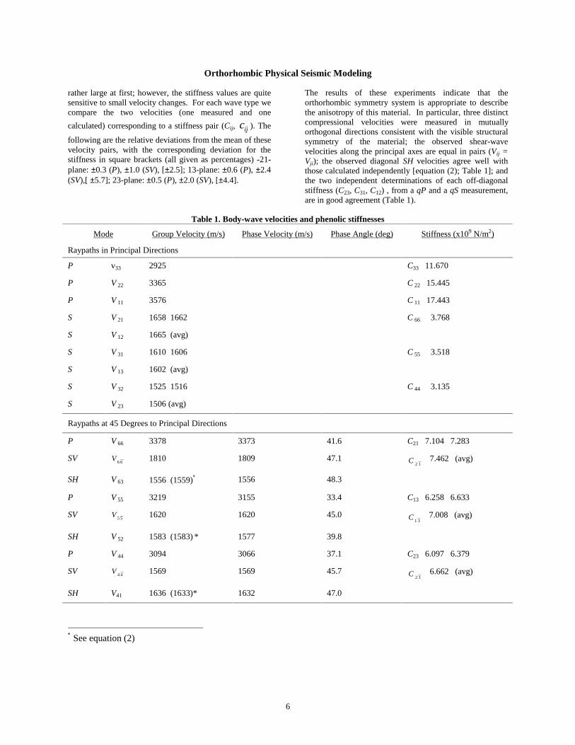
rather large at first; however, the stiffness values are quitesensitive to small velocity changes. For each wave type wecompare the two velocities (one measured and one

calculated) corresponding to a stiffness pair (Cij, jic ). The

following are the relative deviations from the mean of thesevelocity pairs, with the corresponding deviation for thestiffness in square brackets (all given as percentages) -21-plane: ±0.3 (P), ±1.0 (SV), [±2.5]; 13-plane: ±0.6 (P), ±2.4(SV),[ ±5.7]; 23-plane: ±0.5 (P), ±2.0 (SV), [±4.4].

The results of these experiments indicate that theorthorhombic symmetry system is appropriate to describethe anisotropy of this material. In particular, three distinctcompressional velocities were measured in mutuallyorthogonal directions consistent with the visible structuralsymmetry of the material; the observed shear-wavevelocities along the principal axes are equal in pairs (Vij =Vji); the observed diagonal SH velocities agree well withthose calculated independently [equation (2); Table 1]; andthe two independent determinations of each off-diagonalstiffness (C23, C31, C12) , from a qP and a qS measurement,are in good agreement (Table 1).

Table 1. Body-wave velocities and phenolic stiffnesses

Mode Group Velocity (m/s) Phase Velocity (m/s) Phase Angle (deg) Stiffness (x109 N/m2)

Raypaths in Principal Directions

P v33 2925 C33 11.670

P V 22 3365 C 22 15.445

P V 11 3576 C 11 17.443

S V 21 1658 1662 C 66 3.768

S V 12 1665 (avg)

S V 31 1610 1606 C 55 3.518

S V 13 1602 (avg)

S V 32 1525 1516 C 44 3.135

S V 23 1506 (avg)

Raypaths at 45 Degrees to Principal Directions

P V 66 3378 3373 41.6 C21 7.104 7.283

SV66

V 1810 1809 47.112

C 7.462 (avg)

SH V 63 1556 (1559)∗ 1556 48.3

P V 55 3219 3155 33.4 C13 6.258 6.633

SV 55V 1620 1620 45.0

31C 7.008 (avg)

SH V 52 1583 (1583) * 1577 39.8

P V 44 3094 3066 37.1 C23 6.097 6.379

SV 44V 1569 1569 45.7

32C 6.662 (avg)

SH V41 1636 (1633)* 1632 47.0

∗ See equation (2)


7

DISCUSSION

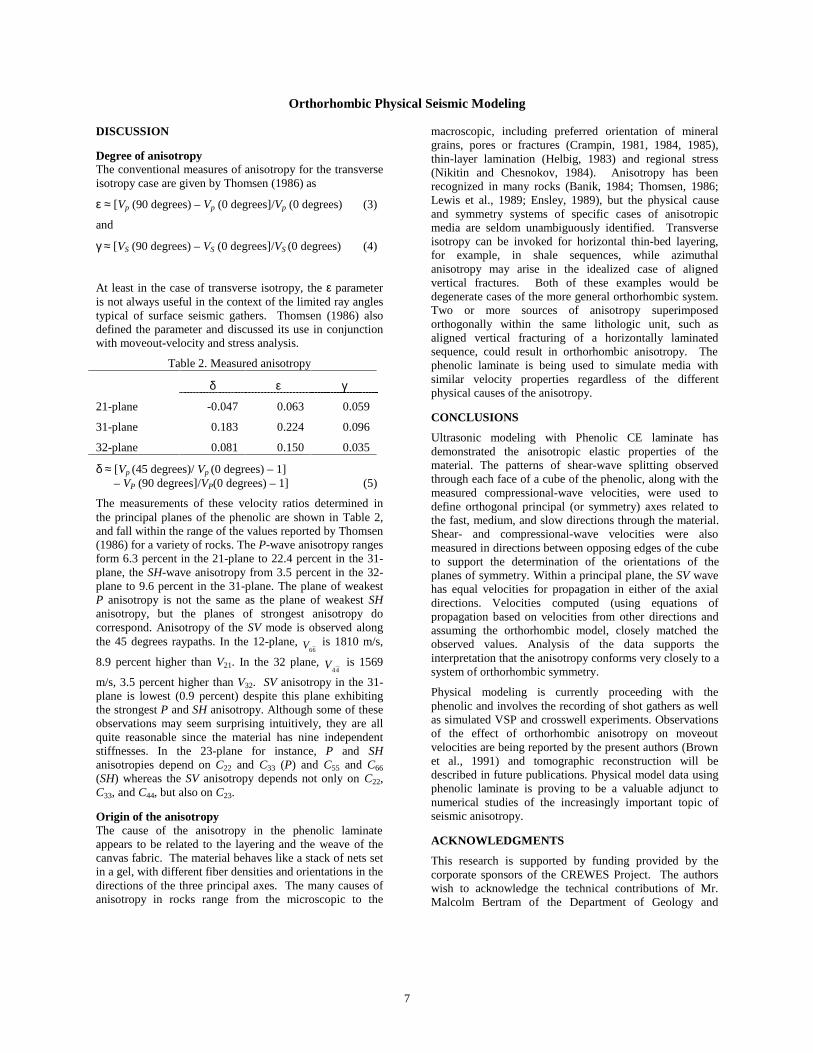
Degree of anisotropyThe conventional measures of anisotropy for the transverseisotropy case are given by Thomsen (1986) as

ε ≈ [Vp (90 degrees) – Vp (0 degrees]/Vp (0 degrees) (3)

and

γ ≈ [VS (90 degrees) – VS (0 degrees]/VS (0 degrees) (4)

At least in the case of transverse isotropy, the ε parameteris not always useful in the context of the limited ray anglestypical of surface seismic gathers. Thomsen (1986) alsodefined the parameter and discussed its use in conjunctionwith moveout-velocity and stress analysis.

Table 2. Measured anisotropy

δ ε γ

21-plane -0.047 0.063 0.059

31-plane 0.183 0.224 0.096

32-plane 0.081 0.150 0.035

δ ≈ [Vp (45 degrees)/ Vp (0 degrees) – 1] – VP (90 degrees]/VP(0 degrees) – 1] (5)

The measurements of these velocity ratios determined inthe principal planes of the phenolic are shown in Table 2,and fall within the range of the values reported by Thomsen(1986) for a variety of rocks. The P-wave anisotropy rangesform 6.3 percent in the 21-plane to 22.4 percent in the 31-plane, the SH-wave anisotropy from 3.5 percent in the 32-plane to 9.6 percent in the 31-plane. The plane of weakestP anisotropy is not the same as the plane of weakest SHanisotropy, but the planes of strongest anisotropy docorrespond. Anisotropy of the SV mode is observed alongthe 45 degrees raypaths. In the 12-plane,

66V is 1810 m/s,

8.9 percent higher than V21. In the 32 plane, 44

V is 1569

m/s, 3.5 percent higher than V32. SV anisotropy in the 31-plane is lowest (0.9 percent) despite this plane exhibitingthe strongest P and SH anisotropy. Although some of theseobservations may seem surprising intuitively, they are allquite reasonable since the material has nine independentstiffnesses. In the 23-plane for instance, P and SHanisotropies depend on C22 and C33 (P) and C55 and C66

(SH) whereas the SV anisotropy depends not only on C22,C33, and C44, but also on C23.

Origin of the anisotropyThe cause of the anisotropy in the phenolic laminateappears to be related to the layering and the weave of thecanvas fabric. The material behaves like a stack of nets setin a gel, with different fiber densities and orientations in thedirections of the three principal axes. The many causes ofanisotropy in rocks range from the microscopic to the

macroscopic, including preferred orientation of mineralgrains, pores or fractures (Crampin, 1981, 1984, 1985),thin-layer lamination (Helbig, 1983) and regional stress(Nikitin and Chesnokov, 1984). Anisotropy has beenrecognized in many rocks (Banik, 1984; Thomsen, 1986;Lewis et al., 1989; Ensley, 1989), but the physical causeand symmetry systems of specific cases of anisotropicmedia are seldom unambiguously identified. Transverseisotropy can be invoked for horizontal thin-bed layering,for example, in shale sequences, while azimuthalanisotropy may arise in the idealized case of alignedvertical fractures. Both of these examples would bedegenerate cases of the more general orthorhombic system.Two or more sources of anisotropy superimposedorthogonally within the same lithologic unit, such asaligned vertical fracturing of a horizontally laminatedsequence, could result in orthorhombic anisotropy. Thephenolic laminate is being used to simulate media withsimilar velocity properties regardless of the differentphysical causes of the anisotropy.

CONCLUSIONS

Ultrasonic modeling with Phenolic CE laminate hasdemonstrated the anisotropic elastic properties of thematerial. The patterns of shear-wave splitting observedthrough each face of a cube of the phenolic, along with themeasured compressional-wave velocities, were used todefine orthogonal principal (or symmetry) axes related tothe fast, medium, and slow directions through the material.Shear- and compressional-wave velocities were alsomeasured in directions between opposing edges of the cubeto support the determination of the orientations of theplanes of symmetry. Within a principal plane, the SV wavehas equal velocities for propagation in either of the axialdirections. Velocities computed (using equations ofpropagation based on velocities from other directions andassuming the orthorhombic model, closely matched theobserved values. Analysis of the data supports theinterpretation that the anisotropy conforms very closely to asystem of orthorhombic symmetry.

Physical modeling is currently proceeding with thephenolic and involves the recording of shot gathers as wellas simulated VSP and crosswell experiments. Observationsof the effect of orthorhombic anisotropy on moveoutvelocities are being reported by the present authors (Brownet al., 1991) and tomographic reconstruction will bedescribed in future publications. Physical model data usingphenolic laminate is proving to be a valuable adjunct tonumerical studies of the increasingly important topic ofseismic anisotropy.

ACKNOWLEDGMENTS

This research is supported by funding provided by thecorporate sponsors of the CREWES Project. The authorswish to acknowledge the technical contributions of Mr.Malcolm Bertram of the Department of Geology and


8

Geophysics and Mr. Eric Gallant of the CREWES Project,both at The University of Calgary. Finally, we would liketo thank Dan Ebrom and Linda Zimmerman for theirknowledgeable reviews of this paper and for theirconstructive suggestions, which have led to an improvedfinal version.

REFERENCES

Aki, K., and Richards, P. G., 1980, Quantitativeseismology: Theory and methods: W. H. Freeman and Co.

Banik, N. C., 1984, Velocity anisotropy of shales and depthestimation in the North Sea basin: Geophysics, 49, 1411-1419.

Brown, R. J., Lawton, D. C., and Cheadle, S. P., 1991,Scaled physical modelling of anisotropic wave propagation:multioffset profiles over an orthorhombic medium:Geophys. J. Internat., in press.

Bullen, K. E., 1963, An introduction to the theory ofseismology: Cambridge University Press.

Crampin, S., 1981, A review of wave motion in anisotropicand cracked elastic-media: Wave Motion, 3, 343-391.-- 1984, An introduction to wave propagation in anisotropicmedia: Geophys. J. Roy. Astr. Soc., 76, 17-28.-- 1985, Evaluation of anisotropy by shear-wave splitting:Geophysics, 50, 142-152.-- 1989, Suggestions for a consistent terminology forseismic anisotropy: Geophys. Prosp., 37, 753-770.

Ebrom, D. A., Tatham, R. ll., Sekharan. K. K., McDonald,J. A., and Gardner, G. H. F., 1990. Hyperbolic traveltimeanalysis of first arrivals in azimuthally anisotropic rnedium:A physical modeling study: Geophysics, 55, 185-191

Ensley, R. A., 1989, Analysis of compressional- and shear-wave seismic data from the Prudhoe Bav Field: The leadingEdge, 8, no. 11, l@13.

Fedorov, F. I., 1968, Theory of elastic waves in crystals:Plenum Press.

Helbig. K., 1983, Elliptical anisotropy - Its significance andmeaning: Geophysics, 48, 825-832.

Keith, C. M., and Crampin, S., 1977, Seismic body wavesin anisotropic media: Reflection and refraction at a planeinterface: Geophys. J. Roy. Astr. Soc., 49, 181-208.

Kendall, J.M., and Thomson, C. J., 1989, A comment onthe form of the geometrical spreading equations, with somenumerical examples of seismic ray tracing ininhomogeneous, anisotropic media: Geophys. J. Internat.,99, 401-413.

Lewis, C., Davis, T. L., Vuillermoz, C., Gurch, M.,Iverson, W., and Schipperijn, A. P., 1989,Three-dimensional imaging of reservoir heterogeneity, Silo Field,Wyoming: 59th Ann. Internat. Mtg., Soc. Expl. Geophys.,Expanded Abstracts, 763-765.

Liu, E., Crampin, S., and Booth, D. C., 1989, Shear-wavesplitting in cross-hole surveys: Modeling: Geophysics, 54,57-65.

Musgrave, M. J. P., 1970, Crystal acoustics: Holden-Day.

Nikitin, L. V., and Chesnokov. E. M., 1984. Wavepropagation in elastic media with stress-inducedanisotropy: Geophys. J. Roy. Astr,. Soc., 76, 129-133.

Nye, J. F., 1985, Physical properties of crystals: OxfordUniversity Press.

Rathore, J. S., Fjaer E., Holt, R. M., and Renlie, L., 1990.Acoustic anisotropy of synthetics with controlled crackgeometries: Presented at the 4th Internat. Workshop onSeismic Anisotropy.

Sayers, C. M., 1988, Stress-induced ultrasonic; wavevelocity anisotropy in fracture rock: Ultrasonics, 26, 311-317.

Tatham, R. H., Matthews, M. D., Sekharan, K. K., Wade,C. J., and Liro, L. M., 1987, A physical model study ofshear-wave splitting and fracture intensity: 57th Ann.Internat. Mtg., Soc. Expl. Geophys., Expanded Abstracts,642-645.

Thomsen, L., 1986, Weak elastic anisotropy: Geophysics,51, 1954-1966.

----- 1988, Reflection seismology over azimuthallyanisotropic media: Geophysics, 53, 304-313.

Vlaar, N. J., 1968. Ray theory for an anisotropicinhomogeneous elastic medium: Bull. Seis. Soc. Am., 58,2053-2072.

Winterstein, D. F., 1990, Velocity anisotropy terminologyfor geophysicists: Geophysics, 55, 1070-1088.

Yale, D. P., and Sprunt, E. S., 1989, Prediction of fracturedirection using shear acoustic anisotropy: The Log Analyst,30, 65-70.

APPENDIX

RELATIONSHIPS AMONG VARIOUS ELASTIC-WAVE PARAMETERS IN AN ANISOTROPICMEDIUM OF ORTHORHOMBIC SYMMETRY

Basic theory and the Kelvin-Christoffel equationsThe equations of motion governing wave propagation in agenerally isotropic elastic medium are given by manyauthors (e.g. Bullen, 1963; Fedorov, 1968; Musgrave,1970- Aki and Richards, 1980; Crampin, 1981, 1984; Nye,1985) For infinitesimal displacements ui, Cartesiancoordinates xi, density ρ, stress tensor σij and body forcesper unit mass gi:

ijiji gu ρσρ += ,&& (A-1)


9

where ",j" denotes the partial derivative with respect to xj

and where the Einstein summation convention (for repeatedindices) applies.

The stress tensor, in terms of the strain tensor εkl and thestiffness tensor Cijkl, is given in accordance with Hooke’slaw by:

klijklij C εσ += , (A-2)

where

( )lkklkl uu ,,21 +=ε . (A-3)

Substituting (A-2) and (A-3) into (A-1), neglecting anybody forces, yields:

0, =− iljkijkl uuC &&ρ . (A-4)

These equations of motion, and their solution formonochromatic plane-wave motion, are considered bymany authors (e.g., Fedorov, 1968; Musgrave, 1970; Keithand Crampin, 1977; Aki and Richards, 1980; Crampin,1981, 1984) but here we follow Musgrave’s treatment mostclosely. We assume harmonic plane-wave displacement,expressed as

( )[ ]txsiApu rrkk −= ωexp , (A-5)

where A is the amplitude factor, pk is the unit polarization(or particle displacement) vector, ω is angular frequency, sr

is the slowness vector, and in this equation only, 1−=i .The slowness vector gives the direction of the wavefrontnormal and may further be written:

rr nvs 1−= , (A-6)

where v is phase velocity and nr is the unit slowness (orwavefront-normal) vector. From equation (A-4), (A-5),and (A-6) one obtains:

( ) 02 =− kikljijkl pvnnC δρ . (A-7)

Thus, the determination of the details of the wave motionhas been cast as an eigenvalue problem in which, havingspecified Cijkl (the stiffnesses of the medium) and nr (thedirection of phase propagation), one can solve for pk (theparticle motion or polarization vector) and three values (ingeneral) for v (phase velocity).

Due to the well known symmetries involved (see e.g.,Musgrave, 1970; Nye, 1985):

kljijiklijlkijkl CCCC === (A-8)

and therefore the matrix (Cijkl nj nl - ρv2σik) is symmetric.This implies in turn that the three eigenvalues obtained forρv2 by setting

02 =− ikljijkl vnnC σρ (A-9)

will be real. (Throughout this appendix vertical bars denote

determinant.)

A further consequence of the symmetries embodied in (A-8) is that there are only 21 independent stiffnesses, Cijkl.Following, e.g., Musgrave (1970), Nye (1985), andThomsen (1986), the fourth-order stiffness tensor may bewritten as a second-order (6 x 6) symmetric matrix:

mnijkl CC →

where

( )

≠=

+−==

ji

j,i

jim

m

if9

if1 (A-10)

and n and kl are analogous to m and ij.

By introducing the so called Kelvin-Christoffel stiffnesses,given by Musgrave (1970) as:

ljijklik nnC=Γ (A-11)

equations (A-7) and (A-9) may be rewritten as:

0

3

2

1

2333231

232

2221

13122

11

=

−ΓΓΓΓ−ΓΓΓΓ−Γ

p

p

p

v

v

v

ρρ

ρ(A-12)

and

02

333231

232

2221

13122

11

=

−ΓΓΓΓ−ΓΓΓΓ−Γ

v

v

v

ρρ

ρ (A-13)

Equations (A-12) and (A-13) are known as the Kelvin-Christoffel equations.

In the case of orthorhombic symmetry only nine of the, ingeneral, 21 indepent stiffnesses, Cmn, are nonzero. The sixindependent Kelvin-Christoffel stiffnesses are then

( )( )( ).66122112

55311331

44233223

332344

2255

2133

442322

2266

2122

552366

2211

2111

CCnn

CCnn

CCnn

CnCnCn

CnCnCn

CnCnCn

+=Γ+=Γ+=Γ

++=Γ++=Γ++=Γ

(A-14)

Propagation along a principal direction

For slowness vector in the 1-direction,

( )0,0,1=jn (A-15)

and equations (A-14) reduce to:


10

=Γ=Γ=Γ=Γ=Γ=Γ

.0123123

5533

6622

1111

C

C

C(A-16)

Equation (A-12) then becomes:

0

00

00

00

3

2

1

233

222

211

=

−Γ−Γ

−Γ

p

p

p

v

v

v

ρρ

ρ(A-17)

For this rather simple case, that of propagation along aprincipal direction, there are three obvious eigenvalueswhich will zero the determinant of the 3 x 3 matrix. Foreach of these, the associated eigenvector pk is thepolarization (or unit-particle-displacement) vector.

The P wave. – Choosing the eigenvalue solution:

0211 =−Γ vρ (A-18)

reduces the three equation of (A-17) to two, namely:

00

0

3

2

1155

1166 =

−

−p

p

CC

CC . (A-19)

The only permissable solution to (A-19) is

032 == pp , (A-20)

since otherwise at least two of the six independentstiffnesses would have to be equal, violating theassumption of orthorhombic symmetry. It follows fromequations (A-16), (A-18), and (A-20) that

( ) ( ) 21/1111and0,0,1 ρCvpk == (A-21)

where v11 denotes that v which applies for propagation(slowness) in the 1-direction with particle motion(polarization) in the 1-direction, that is, the P-wavevelocity.

The S waves.-Choosing each of the other two eigenvaluesolutions leads to the two solutions:

( ) ( ) 21/6612and0,1,0 ρCvpk == (A-22)

and

( ) ( ) 21/5513and1,0,0 ρCvpk == , (A-23)

these representing S waves polarized in the 2- and 3-directions, respectively.

The corresponding velocities and polarizations for thepropagation in the 2- and 3- directions are obtained fromequations (A-21), (A-22), and(A-23) by cyclic variation ofthe indices (1,2,3) and the indices (4,5,6). Since, for theseaxial propagation directions, the wavefront normal and theraypath have the same direction, one could replace v

(phase) with V (group) in equations (A-21), (A-22), and (A-23).

Propagation of 45 degrees to two principal axes or“edge to edge”

Equation (A-21) to (A-23) and their cyclically variedanalogs allow one to determine the six stiffnesses along thediagonal of the Cmn matrix from velocities measured alongprincipal directions. In order to determine the threeindependent off diagonal stiffnesses, one must measurevelocities for raypaths along different directions. The nextsimplest directions to consider would seem to be those inprincipal planes at 45 degrees to each of two principaldirections. We have measured velocities along each suchraypath for the three different polarization.

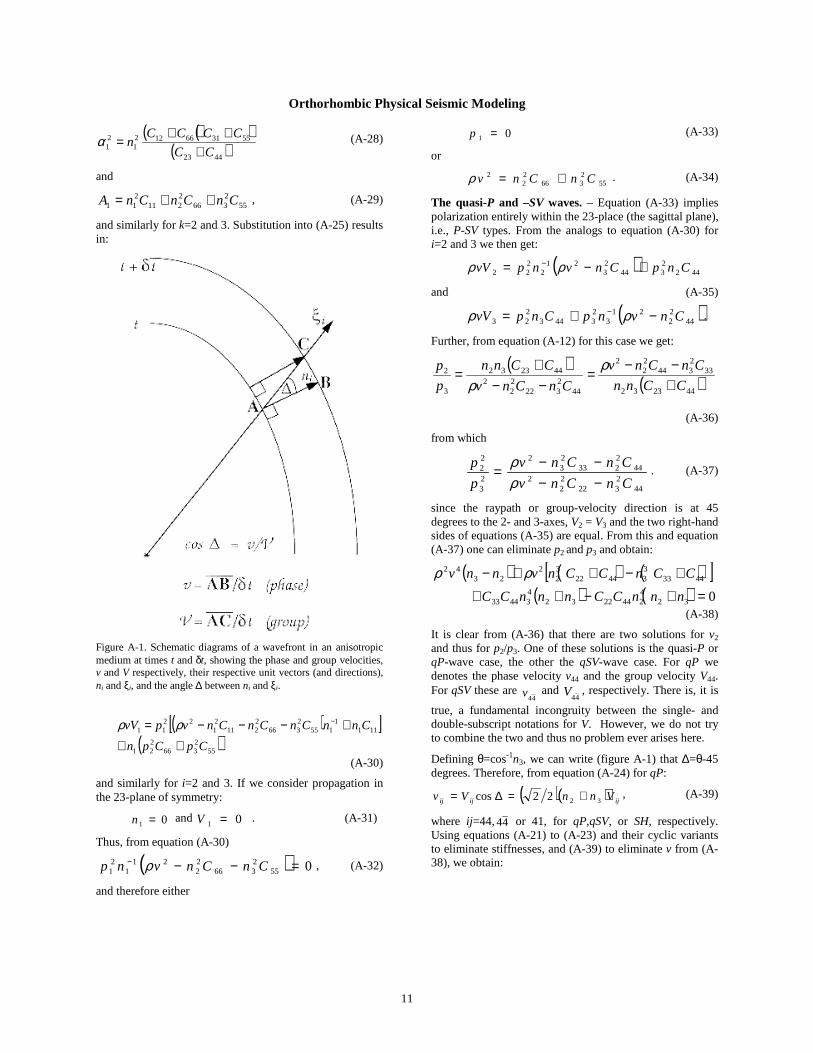
Unfortunately, the raypath or group-velocity direction isnot, in general, the same as the wavefront-normal or phase-velocity direction (Figure A-1). So we cannot make simplesubstitutions for ( )2/2or 0=in in equations (A-14).

We need additional equations that will allow determinationof ni and v from knowledge of ξi ( the unit vector in thegroup-velocity direction; Figure A-1)

Such theory has been dealt with in several works (e.g.Vlaar, 1968; Musgrave, 1970; Kendall and Thomson,1989). Here we take the result from Musgrave (1970) andrefer the reader to the works cited for details. Starting fromthe geometrical relationship (Figure A-1):

iinVv ξ=∆= cos , (A-24)

Musgrave (1970, p.89) gives:

kiik

i n

A

nAv

p

vv

∂∂+

∂∂−

= 2

22

2

2

2

1 ααραρ

, (A-25)

Where

21

ΓΓΓ

=ij

jkik

kα , kji ≠≠ (A-26)

and

summation) (nokkkA Γ= . (A-27)

In equation (A-25), p, α, and A inside brackets should berepresented by their kth components and the products of thebrackets are summed. This notation follows Musgrave(1970) except that, whereas Musgrave use ξi as the group-velocity vector, we use Vi for group velocity and ξi as itsunit vector.

For a medium of orthorhombic symmetry, we get fromequations (A-26), (A-27), and (A-14):


11

( )( )( )4423

5531661221

21 CC

CCCCn

+++

=α (A-28)

and

552366

2211

211 CnCnCnA ++= , (A-29)

and similarly for k=2 and 3. Substitution into (A-25) resultsin:

Figure A-1. Schematic diagrams of a wavefront in an anisotropicmedium at times t and δt, showing the phase and group velocities,v and V respectively, their respective unit vectors (and directions),ni and ξi, and the angle ∆ between ni and ξi.

( )[ ]( )55

2366

221

1111

1552366

2211

21

2211

CpCpn

CnnCnCnCnvpvV

++

+−−−= −ρρ

(A-30)

and similarly for i=2 and 3. If we consider propagation inthe 23-plane of symmetry:

01 =n and 01 =V . (A-31)

Thus, from equation (A-30)

( ) 0552366

22

211

21 =−−− CnCnvnp ρ , (A-32)

and therefore either

01 =p (A-33)

or

552366

22

2 CnCnv +=ρ . (A-34)

The quasi-P and –SV waves. – Equation (A-33) impliespolarization entirely within the 23-place (the sagittal plane),i.e., P-SV types. From the analogs to equation (A-30) fori=2 and 3 we then get:

( ) 4422344

23

212

222 CnpCnvnpvV +−= − ρρ

and (A-35)

( )4422

213

23443

223 CnvnpCnpvV −+= − ρρ .

Further, from equation (A-12) for this case we get:

( )( )442332

332344

22

2

442322

22

2442332

3

2

CCnn

CnCnv

CnCnv

CCnn

p

p

+−−

=−−

+=

ρρ

(A-36)

from which

442322

22

244

2233

23

2

23

22

CnCnv

CnCnv

p

p

−−−−

=ρρ

. (A-37)

since the raypath or group-velocity direction is at 45degrees to the 2- and 3-axes, V2 = V3 and the two right-handsides of equations (A-35) are equal. From this and equation(A-37) one can eliminate p2 and p3 and obtain:

( ) ( ) ( )[ ]( ) ( ) 032

42442232

434433

4433334422

32

223

42

=+−++

+−++−

nnnCCnnnCC

CCnCCnvnnv ρρ

(A-38)

It is clear from (A-36) that there are two solutions for v2

and thus for p2/p3. One of these solutions is the quasi-P orqP-wave case, the other the qSV-wave case. For qP wedenotes the phase velocity v44 and the group velocity V44.For qSV these are

44v and

44V , respectively. There is, it is

true, a fundamental incongruity between the single- anddouble-subscript notations for V. However, we do not tryto combine the two and thus no problem ever arises here.

Defining θ=cos-1n3, we can write (figure A-1) that ∆=θ-45degrees. Therefore, from equation (A-24) for qP:

( )( ) ijijij VnnVv 3222cos +=∆= , (A-39)

where ij=44, 44 or 41, for qP,qSV, or SH, respectively.Using equations (A-21) to (A-23) and their cyclic variantsto eliminate stiffnesses, and (A-39) to eliminate v from (A-38), we obtain:


12

( ) ( ) ( ) ( )[( )] ( ) 04

22

232

2242

223

233

43

223

233

33

223

222

3232

244

22

23

232

444

=−++−

+++−+

VVnVVnVVn

VVnnnVnnnnV ,

(A-40)

in which all of the Vij have been measured experimentally.

Now, since 123

22 =+ nn , equation (A-40) can, in

principle, be solved for n2 and n3. In practice, we determinen2 and n3 by iterative substitution. Knowing n2 and n3 andv44 from equation (A-39), equation (A-36) and (A-37) canbe solved for C23 and the polarization, p2/p3. Similarly,

using ( )qSVV44

in (A-40), we will get different values

(in general) for n2, n3 and44

v ; but assuming the

orthorhombic model to be a reasonable one, we should getthe same result for C23.

The SH wave. – Choosing equation (A-34) instead of (A-33) we have, from (A-14) and (A-31):

11552366

22

241 Γ=+= CnCnvρ (A-41)

so that the Kelvin-Christoffel equations (A-12) result in

( )0,0,1=kp . (A-42)

Incorporating (A-31) and (A-42) into (A-30) and its cyclicvariants yields:

662241 CnVv =ρ and553341 CnVv =ρ . (A-43)

Again applying V2=V3 (for ray at 45 degrees) and equation(A-39), we obtain:

66

55

3

2

C

C

n

n= and

( ) 21212

231

123141

2

VV

VVV

+= . (A-44)

Expression for stiffnesses in terms of group velocities

For completeness, expressions for the nine stiffnesses, forthe case of orthorhombic symmetry, are here summarized.These equations follows directly from (A-21) to A-23), (A-36), and (A-39), as well as their cyclic variant.

===

23333

22222

21111

VC

VC

VC

ρρρ

(A-45)

======

221

21266

213

23155

232

22344

VVC

VVC

VVC

ρρρρρρ

(A-46)

( )[ ]{( )[ ]} 2

23

21223

23

222

22

244

2322

1

233

23

223

23

244

2322

1

3223

VVnVnVnn

VnVnVnnnn

C

ρ

ρ

−−−+

−−+=(A-47a)

( )[ ]{( )[ ]} 2

31

21231

21

233

23

255

2132

1

211

21

231

23

255

2132

1

1331

VVnVnVnn

VnVnVnnnn

C

ρ

ρ

−−−+

−−+= (A-47b)

( )[ ]{( )[ ]} 2

12

21212

23

211

22

266

2212

1

222

22

212

21

266

2212

1

2112

VVnVnVnn

VnVnVnnnn

C

ρ

ρ

−−−+

−−+=. (A-47c)

an in (A-47) Vii(i=4,5,6) may be replaced byiiV .

orthorhombic anisotropy : a physical seismic modeling … · 1 orthorhombic anisotropy: a physical...

Documents