oscillations in damped driven pendulum: a chaotic system · we have proved that oscillations of the...

International Journal of Scientific and Innovative Mathematical Research (IJSIMR)

Volume 3, Issue 10, October 2015, PP 14-27

ISSN 2347-307X (Print) & ISSN 2347-3142 (Online)

www.arcjournals.org

©ARC Page | 14

Oscillations in Damped Driven Pendulum: A Chaotic System

Kulkarni P. R.

P. G. Department of Mathematics,

N. E. S. Science College, Nanded, India. [email protected]

Dr. Borkar V. C.

Department of Mathematics and statistics, Yeshwant Mahavidyalaya, Nanded, India.

[email protected]

Abstract: In this paper, we have discussed the solutions of a system of n differential equations as a continuous

dynamical system. Then we have discussed the nature of oscillations of a damped driven pendulum. We have

analyzed the nature of fixed and periodic points of a damped driven pendulum for certain ranges of parameters.

We have proved that oscillations of the pendulum are chaotic for certain ranges of parameters through the

period doubling phenomenon. For the analysis of the solutions, mathematical softwares like MATLAB and

Phaser Scientific Software are used.

Keywords: chaos, dynamical system, fixed points, orbits, periodic points, stability period doubling

1. INTRODUCTION

A wide range of physical phenomena where there is a change in one quantity that occurs due to a change in one or more quantities can be mathematically modeled in terms of differential equations.

Differential equations can be used to describe the motions of objects like satellites, water molecules in

a stream, waves on strings and surfaces, etc. In this section we will take a review of some basic

terminology associated with a system of differential equations.

1.1 System of Differential Equations [6]

Let be differentiable functions of a variable , usually called as time, on an interval of

the real numbers. Let be functions of and . Then the differential equations

, t),

, t),

.

. (1)

.

, t)

are called as a system of differential equations. This system can also be expressed as

, where , and .

The system , where can depend on the independent variable is called as a non-

autonomous system. Any non-autonomous system (1) with can be written as an autonomous

system (2)

mailto:[email protected]



Kulkarni P. R. & Dr. Borkar V. C.

International Journal of Scientific and Innovative Mathematical Research (IJSIMR) Page 15

with simply by letting and . The fundamental theory for the systems (1)

and (2) does not differ significantly.

1.2 Phase-Plane Analysis

If is defined by and if satisfies the system (1), then is said to be

a solution of the system (1). If and is s solution for all , then is an initial

condition of a solution . As are functions of the variable , it follows that as

increases, traces a curve in called as the trajectory or the orbit and in this case, the space

is called as the phase space of the system. The phase space is completely filled with trajectories since

each point can serve as an initial point. The system is said to be a linear system if

the function is linear. In this case, the system can be expressed as

where is an matrix. The function is also called as a vector field. The vector field

always dictates the velocity vector for each . A picture which shows all qualitatively different

trajectories of the system is called as a phase portrait.[13] A second order differential equation which

can be expressed as a system of two differential equations can be treated as a vector field on a plane

or also called as a phase plane. The general form of a vector field over the plane is

which can be compactly written in vector notations as

, where and . For non-linear systems, it is quite difficult to obtain the trajectories by analytical methods and though the trajectories are obtained by

explicit formulas, they are too complicated to provide the information about the solution. Hence

qualitative behaviors of the trajectories obtained by numerical solution methods are often studied. To

obtain a phase portrait, we plot the variable against the variable and study the qualitative behavior of the solution. A theorem concerning the uniqueness of the solution of a linear system is

stated as follows.

1.3 Theorem (The Fundamental Theorem For Linear Systems) [12]

Let be an matrix. Then for a given , the initial value problem

has a unique solution given by .

Now we state the fundamental theorem for the existence and uniqueness of the solution of a

non-linear system.

1.4 Theorem (The Fundamental Existence-Uniqueness Theorem ) [12]

Let be an open subset of containing and assume that . Then there exists an

such that the initial value problem has a unique solution on the

interval .

1.5 Fixed Point or Stationary Point or Equilibrium Point or Critical Point [6]

A fixed point or an equilibrium point of a system of differential equations is constant solution,

that is, a solution such that for all . If is a critical point, then we identify the

critical point with the vector . From the definition, it is clear that is a fixed point of the system

(1) if .

1.6 Classification of Fixed Points Depending Upon Their Stability [13]

Let be a fixed point of a system .

(i) We say that is an attracting stable fixed point if there is a such that

whenever .

This definition implies that any trajectory that starts near within a distance is guaranteed to

converge to eventually.

(ii) is said to be Liapunov stable if for each , there is a such that



whenever and .

Thus trajectories that start near within remain within for all positive time. Liapunov stability requires that the nearby trajectories stay close for all the time.

(iii) The fixed point is said to be asymptotically stable if it is both attracting and Liapunov

stable.

1.7 Hyperbolic and Nonhyperbolic Fixed Point [13, 19]

A fixed point of a system , where and

is called a hyperbolic fixed point if the real part of the eigenvalues of the

Jacobian matrix at the fixed point are nonzero. If the real part of either

of the eigenvalues are equal to zero, then the fixed point is called as nonhyperbolic.

1.8 Linearization of a Two Dimensional Nonlinear System [19]

Suppose that the nonlinear two dimensional system

(3)

has a critical point , where and are at least quadratic in and . We take a

linear transformation which moves the fixed point to the origin. Let and .

Then the system (3) takes the linearized form

, . (4)

1.9 Hartman's Theorem [19]

Suppose that is a critical point of the system (3). Then there is a neighborhood of this

critical point on which the phase portrait for the nonlinear system resembles that of the linearized

system (4). In other words, there is a curvilinear continuous change of coordinates taking one phase portrait to the other, and in a small region around the critical point, the portraits are qualitatively

equivalent.

1.10 Limit Set [18]

The set of all points that are limit points of a given solution is called the set of ω-limit points, or the

ω-limit set, of the solution . Similarly, we define the set of α-limit points, or the α-limit set, of a

solution to be the set of all points such that for some sequence .

A number of examples of limit set of solution of a differential equation are given in [18]. Now we state the Poincaré-Bendixson theorem which determines all of the possible limiting behaviors of a

planar flow.

1.11 Theorem (Poincaré-Bendixson) [18]

Suppose that is a nonempty, closed and bounded limit set of a planar system of differential

equations that contains no equilibrium point. Then is a closed orbit.

2. OSCILLATIONS OF A PENDULUM SYSTEM

In this section, we will discuss the oscillations of a pendulum subject to a periodic force and a

damping force within certain ranges of parameters. We will discuss different types of oscillations of

the pendulum for different values of the damping force and driven force and prove that the

oscillations are chaotic using the period doubling phenomenon.

2.1 Oscillations in the Absence of Damping Force And Periodic Force

Consider a pendulum of mass and length swinging back and forth. For the present case, suppose

that there is no damping force and no periodic driven force acting on the pendulum. The only force



action on the pendulum is the weight acting downward, where is the acceleration due to gravity.

Let denote the angle made by the pendulum with the normal at time . In this case, the motion of

the pendulum is governed by the second order differential equation

(5)

Because of the trigonometric term , the equation (5) is nonlinear. To find an exact solution of (5)

is not possible. However, numerical solutions can be obtained by different methods. We linearize the

system by considering very small oscillations of the system so that . Thus the system takes

the form . The exact solution of this system is

, (6)

where and are constants which can be determined by using the initial conditions.

The solution (6) is just the equation of a simple harmonic motion. Taking , and

, equation (5) can be written as a system of differential equations given by

, (7)

(8)

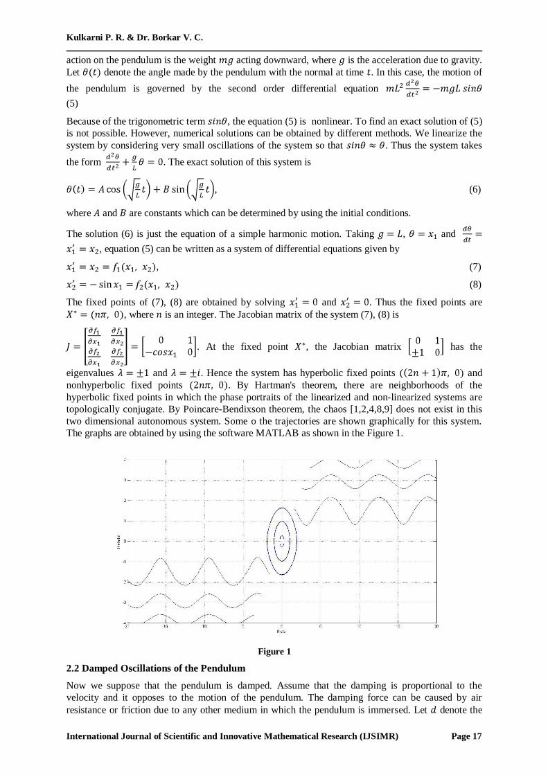
The fixed points of (7), (8) are obtained by solving and . Thus the fixed points are

, where is an integer. The Jacobian matrix of the system (7), (8) is

. At the fixed point , the Jacobian matrix has the

eigenvalues and . Hence the system has hyperbolic fixed points and

nonhyperbolic fixed points . By Hartman's theorem, there are neighborhoods of the

hyperbolic fixed points in which the phase portraits of the linearized and non-linearized systems are

topologically conjugate. By Poincare-Bendixson theorem, the chaos [1,2,4,8,9] does not exist in this

two dimensional autonomous system. Some o the trajectories are shown graphically for this system.

The graphs are obtained by using the software MATLAB as shown in the Figure 1.

Figure 1

2.2 Damped Oscillations of the Pendulum

Now we suppose that the pendulum is damped. Assume that the damping is proportional to the

velocity and it opposes to the motion of the pendulum. The damping force can be caused by air

resistance or friction due to any other medium in which the pendulum is immersed. Let denote the



damping parameter. Then the damping force acting on the pendulum is . Hence the differential

equation of motion of the pendulum becomes

.e. .

For a proper analysis of this equation, we simplify it by the introduction of two variables viz. the

natural frequency and the damping constant . The differential equation of motion of

the pendulum then takes the form

. (9)

With and , equation (9) can be written as a system of differential

equations

, (10)

(11) This is not a linear system, but as discussed in the earlier case where there is no

damping, this system is almost linear [6] at the origin. The linearized system

, (12)

(13)

has the associated matrix . The eigenvalues of this matrix are given by

and . The nature of the fixed point O=(0, 0) depends

upon the values of and . Note that the real parts of and are negative so that the solutions of

the linear system (12), (13) are asymptotically stable. Hence by Hartman's theorem, in some neighborhoods of the origin, the solutions of the nonlinear damped system (10), (11) are stable at the

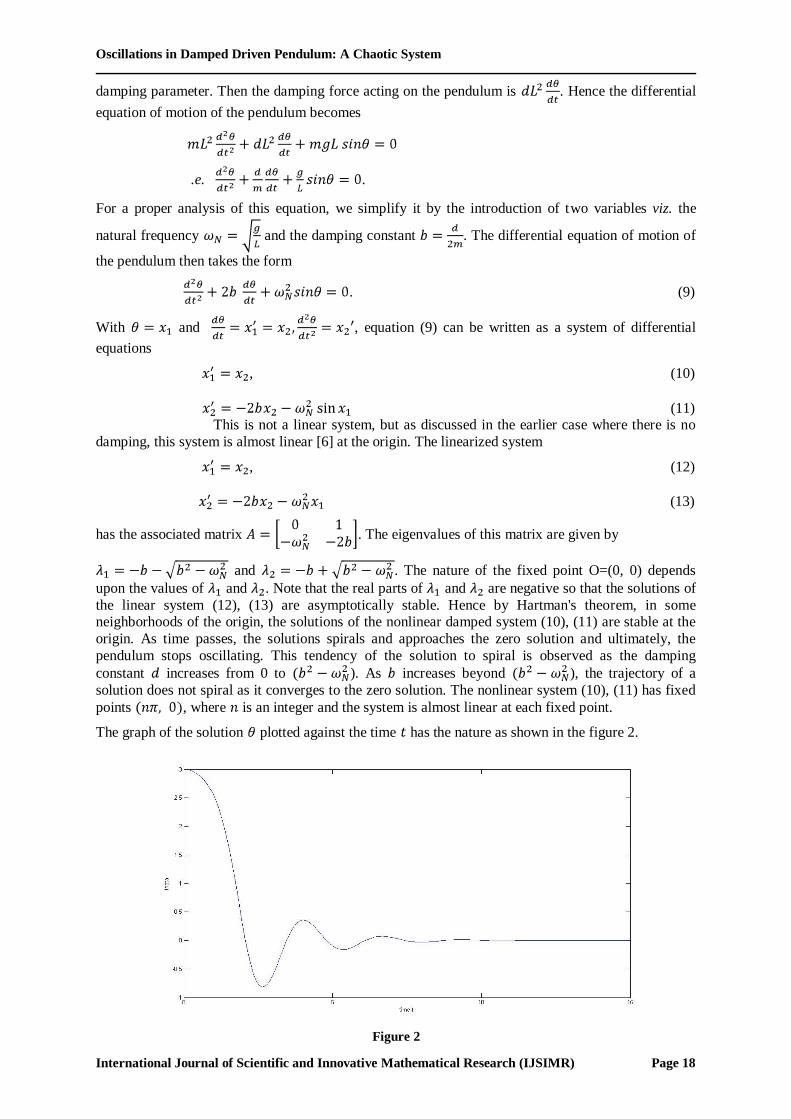
origin. As time passes, the solutions spirals and approaches the zero solution and ultimately, the

pendulum stops oscillating. This tendency of the solution to spiral is observed as the damping

constant increases from 0 to ). As increases beyond ), the trajectory of a

solution does not spiral as it converges to the zero solution. The nonlinear system (10), (11) has fixed

points , where is an integer and the system is almost linear at each fixed point.

The graph of the solution plotted against the time has the nature as shown in the figure 2.

Figure 2



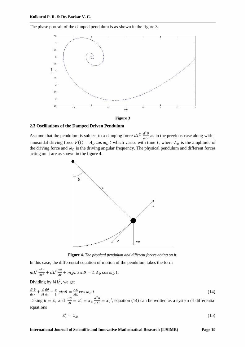
The phase portrait of the damped pendulum is as shown in the figure 3.

Figure 3

2.3 Oscillations of the Damped Driven Pendulum

Assume that the pendulum is subject to a damping force as in the previous case along with a

sinusoidal driving force which varies with time , where is the amplitude of

the driving force and is the driving angular frequency. The physical pendulum and different forces

acting on it are as shown in the figure 4.

Figure 4. The physical pendulum and different forces acting on it.

In this case, the differential equation of motion of the pendulum takes the form

.

Dividing by , we get

(14)

Taking and , equation (14) can be written as a system of differential

equations

, (15)



(16)

The system of equations (15), (16) appears to be a two dimensional phase-plane system and one may

conclude by Poincare-Bendixson theorem that the chaos is not possible in the oscillations of the

pendulum, but note that the system is non-autonomous and it can be made a three dimensional

autonomous system simply by adding one more variable so that the system can be

expressed as

,

,

Thus the Poincare-Bendixson theorem is not applicable and chaos may be observed in the system.

Denoting , and , the system (15), (16) can be expressed as

, (17)

(18)

This type of system of equations appears in John Taylor's Classical Mechanics. [20] We choose

so that the period of the driving force becomes . The chaos can be observed in the

system if is close to . It can be verified that the much erratic oscillations of the pendulum are

observed when as compared to the case . We will keep the values of the

parameters , and as constants and vary the parameter in search of the chaos. As suggested

by John R. Taylor, we will use the parameter values , , and let vary. The

period doubling phenomenon has been one of the important characterization of chaotic dynamical

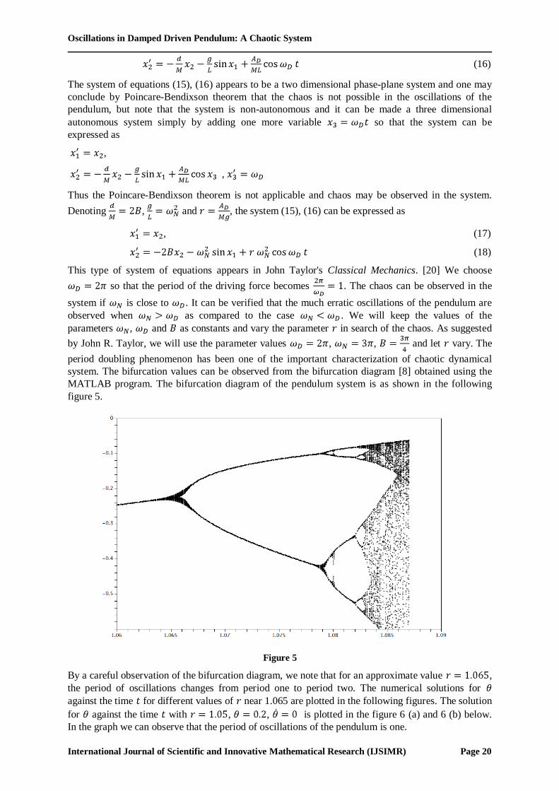
system. The bifurcation values can be observed from the bifurcation diagram [8] obtained using the

MATLAB program. The bifurcation diagram of the pendulum system is as shown in the following

figure 5.

Figure 5

By a careful observation of the bifurcation diagram, we note that for an approximate value ,

the period of oscillations changes from period one to period two. The numerical solutions for

against the time for different values of near 1.065 are plotted in the following figures. The solution

for against the time with , , is plotted in the figure 6 (a) and 6 (b) below.

In the graph we can observe that the period of oscillations of the pendulum is one.



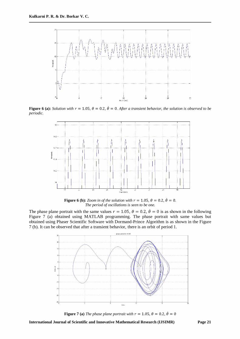
Figure 6 (a): Solution with , , . After a transient behavior, the solution is observed to be periodic.

Figure 6 (b): Zoom in of the solution with , , .

The period of oscillations is seen to be one.

The phase plane portrait with the same values , , is as shown in the following Figure 7 (a) obtained using MATLAB programming. The phase portrait with same values but

obtained using Phaser Scientific Software with Dormand-Prince Algorithm is as shown in the Figure

7 (b). It can be observed that after a transient behavior, there is an orbit of period 1.

Figure 7 (a) The phase plane portrait with , ,



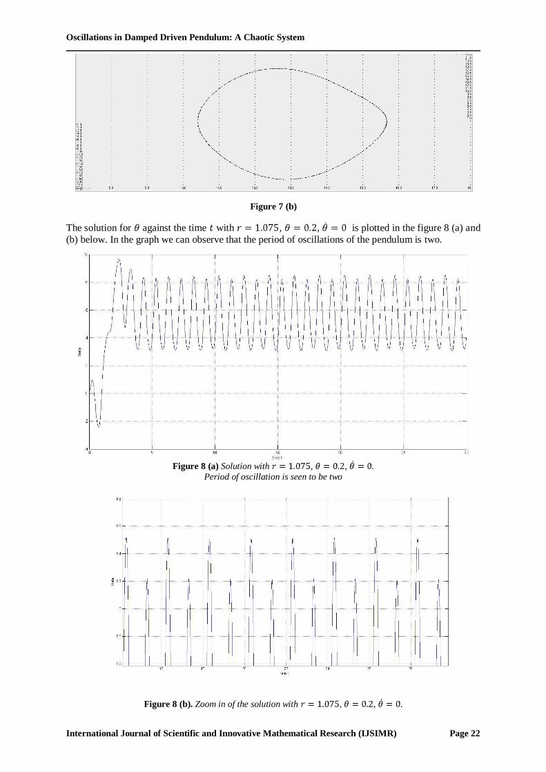
Figure 7 (b)

The solution for against the time with , , is plotted in the figure 8 (a) and

(b) below. In the graph we can observe that the period of oscillations of the pendulum is two.

Figure 8 (a) Solution with , , .

Period of oscillation is seen to be two

Figure 8 (b). Zoom in of the solution with , , .



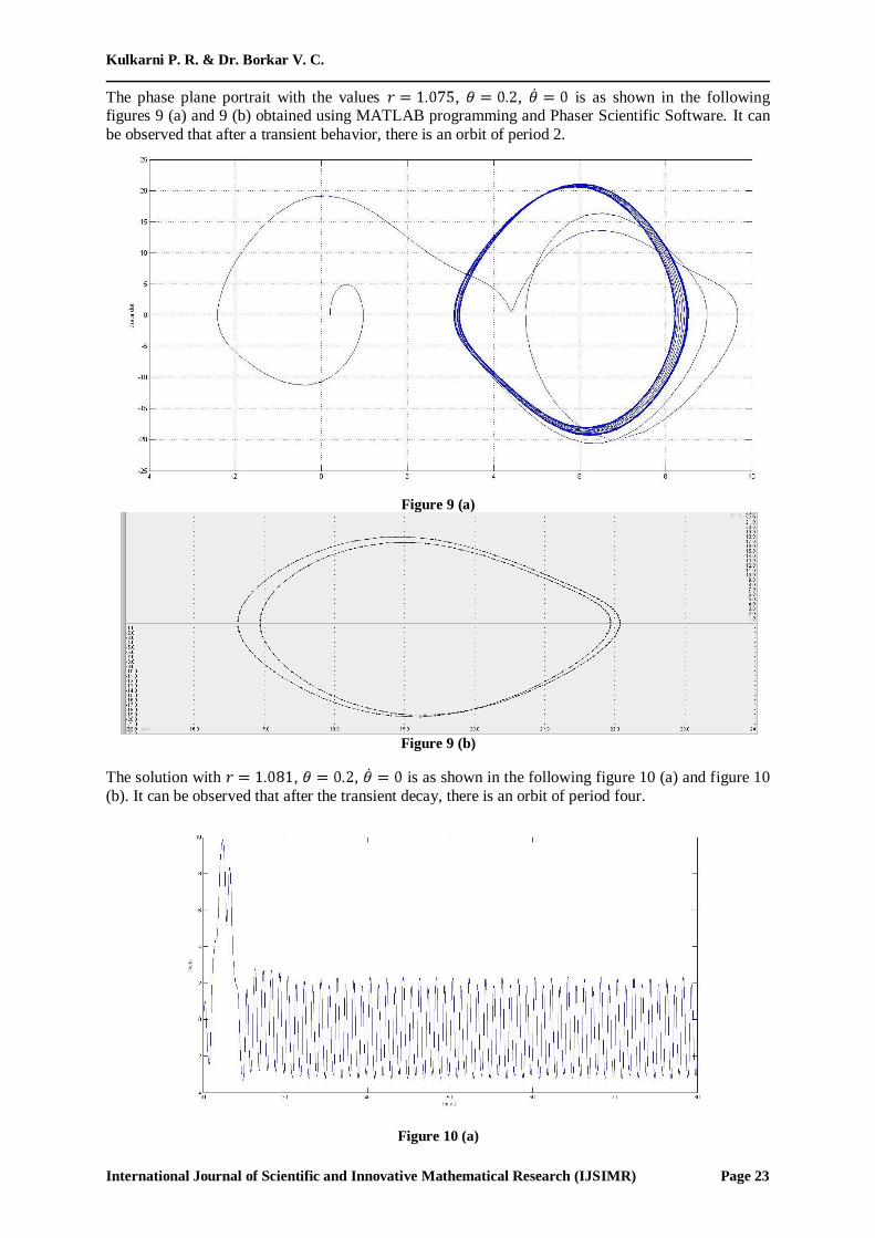
The phase plane portrait with the values , , is as shown in the following figures 9 (a) and 9 (b) obtained using MATLAB programming and Phaser Scientific Software. It can

be observed that after a transient behavior, there is an orbit of period 2.

Figure 9 (a)

Figure 9 (b)

The solution with , , is as shown in the following figure 10 (a) and figure 10

(b). It can be observed that after the transient decay, there is an orbit of period four.

Figure 10 (a)



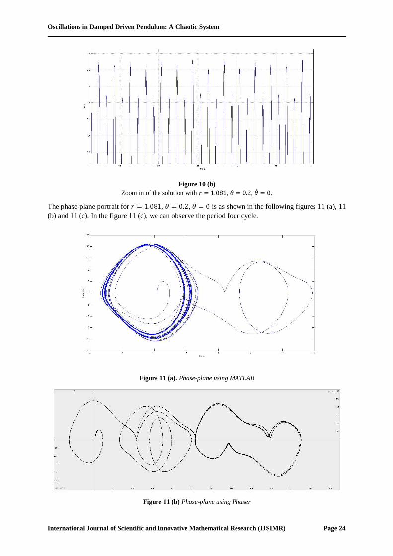
Figure 10 (b)

Zoom in of the solution with , , .

The phase-plane portrait for , , is as shown in the following figures 11 (a), 11

(b) and 11 (c). In the figure 11 (c), we can observe the period four cycle.

Figure 11 (a). Phase-plane using MATLAB

Figure 11 (b) Phase-plane using Phaser



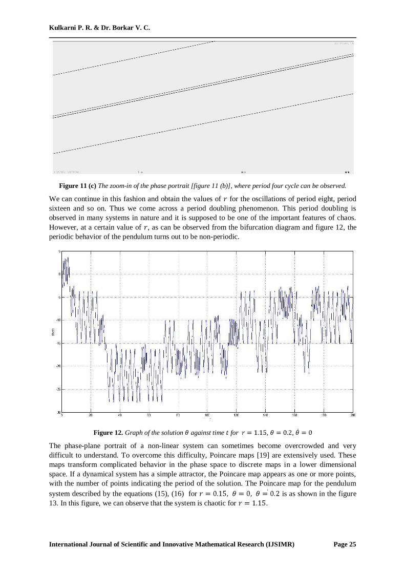
Figure 11 (c) The zoom-in of the phase portrait [figure 11 (b)], where period four cycle can be observed.

We can continue in this fashion and obtain the values of for the oscillations of period eight, period

sixteen and so on. Thus we come across a period doubling phenomenon. This period doubling is

observed in many systems in nature and it is supposed to be one of the important features of chaos.

However, at a certain value of , as can be observed from the bifurcation diagram and figure 12, the

periodic behavior of the pendulum turns out to be non-periodic.

Figure 12. Graph of the solution against time for , ,

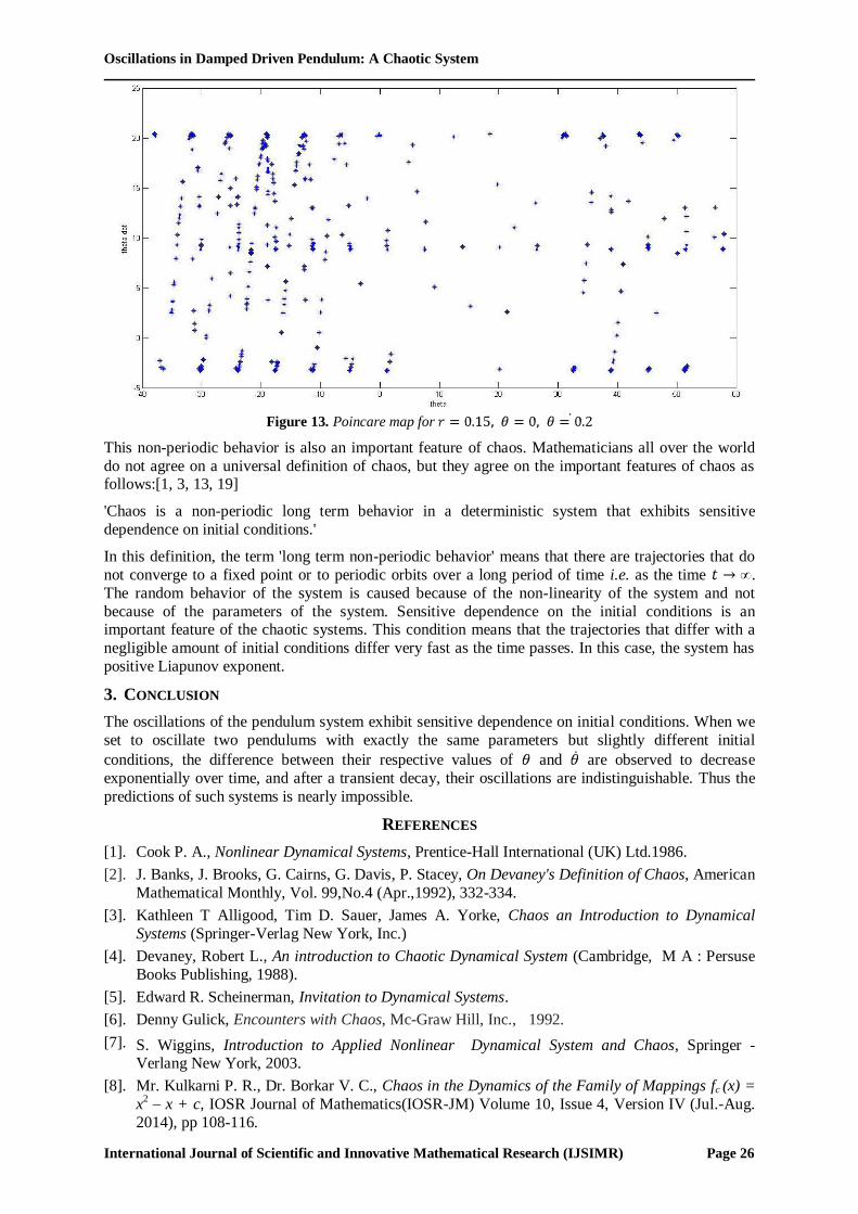
The phase-plane portrait of a non-linear system can sometimes become overcrowded and very

difficult to understand. To overcome this difficulty, Poincare maps [19] are extensively used. These

maps transform complicated behavior in the phase space to discrete maps in a lower dimensional

space. If a dynamical system has a simple attractor, the Poincare map appears as one or more points,

with the number of points indicating the period of the solution. The Poincare map for the pendulum

system described by the equations (15), (16) for is as shown in the figure

13. In this figure, we can observe that the system is chaotic for .



Figure 13. Poincare map for

This non-periodic behavior is also an important feature of chaos. Mathematicians all over the world

do not agree on a universal definition of chaos, but they agree on the important features of chaos as follows:[1, 3, 13, 19]

'Chaos is a non-periodic long term behavior in a deterministic system that exhibits sensitive

dependence on initial conditions.'

In this definition, the term 'long term non-periodic behavior' means that there are trajectories that do

not converge to a fixed point or to periodic orbits over a long period of time i.e. as the time .

The random behavior of the system is caused because of the non-linearity of the system and not

because of the parameters of the system. Sensitive dependence on the initial conditions is an important feature of the chaotic systems. This condition means that the trajectories that differ with a

negligible amount of initial conditions differ very fast as the time passes. In this case, the system has

positive Liapunov exponent.

3. CONCLUSION

The oscillations of the pendulum system exhibit sensitive dependence on initial conditions. When we

set to oscillate two pendulums with exactly the same parameters but slightly different initial

conditions, the difference between their respective values of and are observed to decrease

exponentially over time, and after a transient decay, their oscillations are indistinguishable. Thus the

predictions of such systems is nearly impossible.

REFERENCES

[1]. Cook P. A., Nonlinear Dynamical Systems, Prentice-Hall International (UK) Ltd.1986.

[2]. J. Banks, J. Brooks, G. Cairns, G. Davis, P. Stacey, On Devaney's Definition of Chaos, American

Mathematical Monthly, Vol. 99,No.4 (Apr.,1992), 332-334.

[3]. Kathleen T Alligood, Tim D. Sauer, James A. Yorke, Chaos an Introduction to Dynamical

Systems (Springer-Verlag New York, Inc.)

[4]. Devaney, Robert L., An introduction to Chaotic Dynamical System (Cambridge, M A : Persuse

Books Publishing, 1988).

[5]. Edward R. Scheinerman, Invitation to Dynamical Systems.

[6]. Denny Gulick, Encounters with Chaos, Mc-Graw Hill, Inc., 1992.

[7]. S. Wiggins, Introduction to Applied Nonlinear Dynamical System and Chaos, Springer - Verlang New York, 2003.

[8]. Mr. Kulkarni P. R., Dr. Borkar V. C., Chaos in the Dynamics of the Family of Mappings fc (x) =

x2 – x + c, IOSR Journal of Mathematics(IOSR-JM) Volume 10, Issue 4, Version IV (Jul.-Aug.

2014), pp 108-116.



[9]. Kulkarni P. R. and Borkar V. C., Topological conjugacy and the Chaotic Nature of the Family of Mappings fc (x) = x

2 – x + c, International Journal of Scientific and Innovative Mathematical

Research (IJSIMR), Volume 2, Issue 11, November 2014 PP 868-875.

[10]. George D. Birkhoff, Dynamical Systems, American Mathematical Society Colloquium

Publications, Volulme IX.

[11]. Karl-Hienz Beeker, Michael Dorfer, Dynamical Systems and Fractals, Cambridge University

Press, Cambridge.

[12]. Lawrence Perko, Differential Equations and Dynamical Systems, Third Edition, Springer-Verlag,

New York Inc.

[13]. Stevan H. Strogatz, Non-linear Dynamics and Chaos, Perseus Books Publishing, LLC.

[14]. Garnett P. Williams, Chaos Theory Tamed, Joseph Henry Press, Washington D.C.,1997.

[15]. Marian Gidea, Constantin P. Niculescu, Chaotic Dynamical Systems an Introduction, Craiova Universitaria Press, 2002.

[16]. Gerald Teschl, Ordinary Differential Equations and Dynamical Systems, American

Mathematical Society.

[17]. Frank C. Hoppensteadt, Analysis and Simulation of Chaotic Systems, Second Edition, Springer-

Verlag, New York Inc.

[18]. Morris W. Hirsch, Stephan Smale, Robert L. Devaney, Differential Equations, Dynamical

Systems and An Introduction to Chaos, Second Edition, Elsevier Academic Press, 2004.

[19]. Stephan Lynch, Dynamical Systems with Applications using MATLAB, Second Edition, Springer

International Publishing, Switzerland, 2004,2014.

[20]. John R. Taylor, Classical Mechanics, IInd Edition, University Science Books, 2005.

AUTHORS’ BIOGRAPHY

Kulkarni P. R. is working as an assistant professor at the department of

Mathematics, N. E. S. Science college, Nanded (Maharashtra). He is a research

student working in the Swami Ramanand Teerth Marathwada University, Nanded. His area of research is dynamical systems and it’s applications in various fields.

Dr. V. C. Borkar, working as Associate Professor and Head in Department of

Mathematics and Statistics Yeshwant Mahavidyalaya Nanded , Under Swami

Ramanand Teerth Marathwada University, Nanded (M.S) India. His area of specialization is functional Analysis. He has near about 16 year research

experiences. He completed one research project on Dynamical system and their

applications. The project was sponsored by UGC, New Delhi.

oscillations in damped driven pendulum: a chaotic system · we have proved that oscillations of the...

Documents