ostrich documentation and user · pdf fileostrich is a model-independent and multi-algorithm...
TRANSCRIPT

OSTRICH Documentation and User Guide
OSTRICH – An Optimization Software Toolkit for Research Involving Computational Heuristics
Documentation and User’s Guide
by
L. Shawn Matott, Ph.D. State University of New York at Buffalo
Center for Computational Research
OSTRICH Documentation and User Guide
2
Acknowledgements Funding for the creation of this user manual was provided by Environment Canada under
contract number K3D35-14-0487R. The Dynamically Dimensioned Search (DDS) algorithm was developed by Professor Bryan Tolson and implemented in C/C++ code by Professor James Craig. Both James and Bryan are currently at the University of Waterloo. Professor Craig also provided routines for generating normally distributed random variables. Other variants of the DDS family of algorithms were ported to OSTRICH using C/C++ and FORTRAN implementations provided by Professor Tolson’s research group. Hyper volume calculations within the Pareto Archived DDS code have been adapted from original C++ source developed by Nicola Beume at the University of Dortmund. The Shuffled Complex Evolution (SCE) algorithm was ported from the original FORTRAN implementation of Dr. Qingyun Duan. All other algorithm implementations are based on published descriptions and were coded primarily by L. Shawn Matott. The basic object-oriented and model-independent structure of OSTRICH is based off of a code known as MACT (Multi-Algorithm Calibration Tool) that was developed by Vijaykumar Raghavan while at the University at Buffalo and under the supervision of Professor Alan J. Rabideau. Portions of the genetic algorithm and simulated annealing implementations in OSTRICH were ported from Mr. Raghavan’s MACT code.
Preface OSTRICH is a model-independent and multi-algorithm optimization and calibration tool.
It can be used for weighted non-linear least-squares calibration of model parameters, or for constrained optimization of a set of design variables according to a user-defined objective or cost function. Both single and multi-objective optimization are supported along with multi-criteria calibration. Parameters to be calibrated or optimized can be log-transformed or computed as functions of other parameters. OSTRICH is also capable of computing an extensive set of post-calibration statistics, include confidence intervals, parameter correlation, tests of normality and non-linearity, and measures of observation influence and parameter sensitivity. OSTRICH can be configured to operate with any modeling program that utilizes text-based input and output file formats. Additional I/O formats that are supported include the MS Access database and netcdf formats. Executable versions of OSTRICH are available for both Windows and Linux-based computing environments. A parallel version of OSTRICH (OstrichMPI), utilizing the industry standard MPI interface, is also available in both Windows and Linux. Linux builds of OstrichMPI are available for both the OpenMPI and Intel-MPI implementations of the MPI standard. The Windows-based OstrichMPI uses a file-based implementation of the MPI standard developed by the author (L. Shawn Matott, [email protected]).
Table of Contents 1. Introduction ......................................................................................................................... 6
1.1. Calibration and Optimization Algorithms .......................................................................... 6

OSTRICH Documentation and User Guide
3
1.2. Regression Statistics and Diagnostics ............................................................................... 10
2. ostIn.txt – the OSTRICH Input File .................................................................................. 11
2.1. Comments ......................................................................................................................... 12
2.2. Case Sensitivity ................................................................................................................. 13
2.3. ostIn – Basic Configuration .............................................................................................. 13
2.4. ostIn – File Pairs ............................................................................................................... 17
2.5. ostIn – Extra Files ............................................................................................................. 18
2.6. ostIn – Extra Directories ................................................................................................... 19
2.7. ostIn – Real-valued Parameters ........................................................................................ 19
2.8. ostIn – Integer Parameters ................................................................................................ 21
2.9. ostIn – Combinatorial Parameters ..................................................................................... 21
2.10. ostIn – Tied Parameters .................................................................................................... 22
2.11. ostIn – Special Parameters (pre-emption) ......................................................................... 25
2.12. ostIn – Initial Parameters .................................................................................................. 27
2.13. ostIn – Parameter Correction ............................................................................................ 27
2.14. ostIn – Observations ......................................................................................................... 29
2.15. ostIn – Response Variables ............................................................................................... 33
2.16. ostIn – Tied Response Variables....................................................................................... 34
2.17. ostIn – Type Conversion (MS Access, netcdf) ................................................................. 35
2.18. ostIn – Search Algorithms ................................................................................................ 37
2.18.1. Bisection Algorithm ................................................................................................ 37
2.18.2. Fletcher-Reeves....................................................................................................... 38
2.18.3. Gauss-Marquardt-Levenberg .................................................................................. 38
2.18.4. Multi-Start GML with Trajectory Repulsion .......................................................... 39
2.18.5. Grid-based Exhaustive Search ................................................................................ 40
2.18.6. Powell's Algorithm ................................................................................................. 41
2.18.7. Steepest Descent ..................................................................................................... 41
2.18.8. Asynchronous Parallel Particle Swarm Optimization............................................. 41
2.18.9. Particle Swarm Optimization (PSO) ....................................................................... 43
OSTRICH Documentation and User Guide
4
2.18.10. PSO with GML Polishing ....................................................................................... 43
2.18.11. Balanced Exploration-Exploitation Random Search .............................................. 43
2.18.12. Binary- and Real-coded Genetic Algorithms (BGA and RGA) ............................. 44
2.18.13. Combinatorial (Discrete) Simulated Annealing...................................................... 44
2.18.14. Simulated Annealing ............................................................................................... 45
2.18.15. Vanderbilt-Louie Simulated Annealing .................................................................. 46
2.18.16. Discrete DDS .......................................................................................................... 47
2.18.17. Dynamically Dimensioned Search (DDS) .............................................................. 48
2.18.18. Asynchronous Parallel DDS ................................................................................... 48
2.18.19. Shuffled Complex Evolution (SCE) ....................................................................... 50
2.18.20. Sampling Algorithm (Big Bang - Big Crunch) ....................................................... 51
2.19. ostIn – Uncertainty-based Search Algorithms .................................................................. 51
2.19.1. DDS for Approximation of Uncertainty ................................................................. 51
2.19.2. Generalized Likelihood Uncertainty Estimation (GLUE) ...................................... 53
2.19.3. Metropolis-Hastings Markov Chain Monte Carlo (MCMC) .................................. 54
2.19.4. Rejection Sampling ................................................................................................. 55
2.20. ostIn – Multi-Objective Search Algorithms ...................................................................... 56
2.20.1. Pareto Archived DDS (PADDS) ............................................................................. 56
2.20.2. Asynchronous Parallel PADDS .............................................................................. 57
2.20.3. Simple Multi-Objective Optimization Test Heuristic (SMOOTH) ........................ 57
2.21. ostIn – Math and Stats....................................................................................................... 57
2.22. ostIn – Line Search ........................................................................................................... 61
2.23. ostIn – General-purpose Constrained Optimization Platform (GCOP) ............................ 61
2.24. ostIn – Constraints ............................................................................................................ 62
3. Running Ostrich ................................................................................................................ 63
3.1.1. Using Weighted Sum of Squared Errors (WSSE) Calibration ................................... 64
3.1.2. Using the General Constrained Optimization Platform (GCOP) ............................... 64
3.2. Serial (Single Processor) Execution .................................................................................. 64
3.3. Multi-core Parallel Execution in Windows....................................................................... 64

OSTRICH Documentation and User Guide
5
3.4. Distributed or Multi-core Parallel Execution in Linux ..................................................... 65
3.5. Aborting an Ostrich Run ................................................................................................... 66
3.6. Restarting an Ostrich Run ................................................................................................. 66
4. Ostrich Output Files .......................................................................................................... 66
4.1. OstOutput – Main Output File .......................................................................................... 67
4.2. OstOutput – Statistical Output .......................................................................................... 67
4.2.1. Observation Residuals ................................................................................................ 67
4.2.2. Error Variance and Standard Error of the Regression ................................................ 67
4.2.3. Parameter Variance-Covariance and Correlation ....................................................... 67
4.2.4. Confidence Intervals ................................................................................................... 67
4.2.5. Model Linearity .......................................................................................................... 67
4.2.6. Normality of Residuals ............................................................................................... 68
4.2.7. Influential Observations ............................................................................................. 68
4.2.8. Parameter Sensitivities ............................................................................................... 68
4.2.9. Matrices ...................................................................................................................... 68
4.3. OstError – OSTRICH Error and Warning Messages ........................................................ 68
4.4. OstExeOut – Redirected Model Output ............................................................................ 69
4.5. OstModel – Model Run Record ........................................................................................ 69
5. Examples ........................................................................................................................... 69
5.1. Demo #1 – Calibrating SPLIT Groundwater Flow Model ............................................... 69
5.2. Demo #2 – Pump-and-Treat Optimization ....................................................................... 70
5.3. Demo #3 – Optimizing a BIGFOOT Benchmark ............................................................. 70
5.4. Demo #4 – Calibrating a TUSWAMP Watershed Model ................................................ 70
5.5. Demo #5 – Simple Pre-Emption Demonstration .............................................................. 71
5.6. Demo #6 – Cantilever Beam Multi-Objective Optimization ............................................ 71
5.7. Demo #7 – Multi-Criteria MODFLOW Calibration ......................................................... 71
5.8. Demo #8 – Warm Start Example ...................................................................................... 71
5.9. Demo #9 – Uncertainty-based Calibration Example ........................................................ 72
6. References ......................................................................................................................... 72

OSTRICH Documentation and User Guide
6
1. Introduction OSTRICH is a model-independent program that automates the processes of model
calibration and design optimization without requiring the user to write any additional software. Typically, users only need to fill out a few required portions of the OSTRICH input file (i.e. ostIn.txt) and create template model input files. Users may also activate and configure a variety of optional features, including: parallel processing, model pre-emption, algorithm restarts, parameter statistics and regression diagnostics, telescoping parameter bounds, predictive uncertainty, non-ASCII model I/O, and user-defined initial parameter sets. Finally, users with skill in code or script development (e.g. C/C++, FORTRAN, Java, R, MATLAB, Python, bash/bat, etc.) may also wish to take advantage of OSTRICH’s parameter correction feature. It allows users to correct candidate parameter sets based on rules-of-thumb or expert judgment that would otherwise be difficult to encapsulate as optimization constraints.
The remainder of this manual describes the configuration and usage of OSTRICH. Sections 1.1 and 1.2 provide brief summaries of the currently supported optimization and calibration algorithms (Section 1.1), and regression statistics and diagnostics (Section 1.2). Sections 2 through 2.24 describe the OSTRICH input file and its various configuration sections. The majority of these sections are optional and others will only be processed when a specific algorithm, objective function (i.e. calibration vs. constrained optimization vs. multi-objective optimization), or feature is activated. Section 3 provides guidance on running OSTRICH in serial or parallel, and Section 4 describes various output files generated by OSTRICH. Finally, Section 5 reviews the set of examples that accompany the OSTRICH distribution and provides instructions for running them on a Windows-based machine.
1.1. Calibration and Optimization Algorithms OSTRICH implements numerous algorithms. Some of these algorithms are deterministic
local search methods, others are heuristic global search methods that incorporate elements of structured randomness, and others act as samplers that seek to delineate parameter probability distributions rather than just identifying a single optimal parameter set. While most of these algorithms are suitable for both calibration and optimization problems, one deterministic algorithm (i.e. Levenberg-Marquardt) is tailored to non-linear least-squares calibration problems. Additionally, two algorithms (i.e. Pareto Archive Dynamically Dimensioned Search and the Simple Multi-Objective Optimization Test Heuristic) are suitable for multi-objective optimization or multi-criteria calibration. Finally, several sampling-based algorithms (i.e. Generalized Likelihood Uncertainty Estimation, Rejection Sampling, and Metropolis-Hastings Markov Chain Monte Carlo) are suitable for uncertainty-based calibration. Overall, these algorithms provide the user with a fair degree of flexibility and enable OSTRICH to tackle a variety of linear and non-linear problems. Furthermore, these problems can have continuously
OSTRICH Documentation and User Guide
7
varying (i.e. real-valued) parameters, combinatorial parameters, integer parameters, or a mixture of continuous, combinatorial and integer parameters.
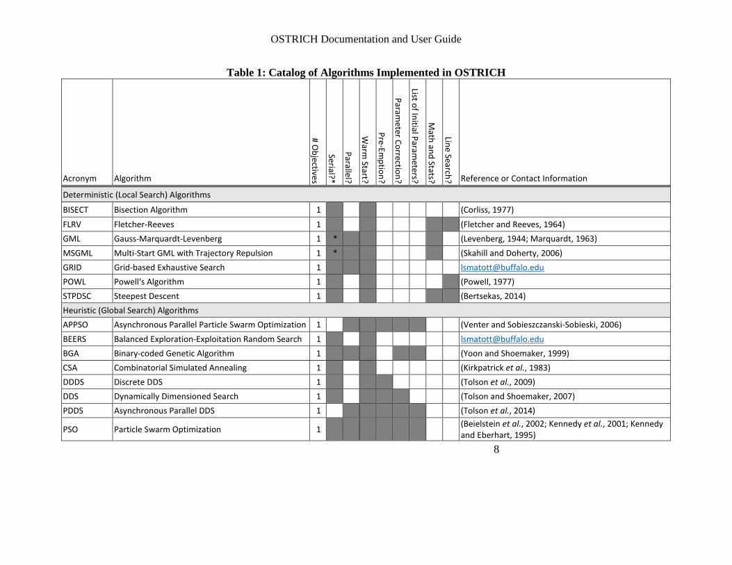
Table 1 summarizes each algorithm implemented in OSTRICH along with appropriate references for detailed descriptions. Algorithms where only contact information is provided are unpublished experimental algorithms and should be used with caution. Some algorithms have been validated against reference implementations. These algorithms include: DDS, PADDS, PSO, GML, BGA, RGA, SA, FLRV, POWL, STPDSC, and SCE. C/C++ programmers will find it straightforward to extend OSTRICH to include additional search algorithms. Doing so involves extension of an abstract base class (AlgorithmABC) that defines a minimum set of required search algorithm functions, including: Calbrate(), Optimize(), WriteMetrics(), WarmStart(), and Destroy(). These functions typically utilize additional classes that encapsulate parameters (i.e. ParameterGroup), models (i.e. ModelABC), and objective functions (i.e. ObjectiveFunction) which are dynamically instantiated based on a user-supplied configuration file.
As shown in Listing 5, OSTRICH supports a special ProgramType named “ModelEvaluation”. OSTRICH will process the parameter sets listed in the “InitParams” groups (see Section 2.12) when this program type is selected. In this way, users may request evaluation of a specific set of parameters independent of any search algorithm embedded within OSTRICH. For example, such parameter sets could be generated as part of a sensitivity or uncertainty analysis procedure that is run using an external spreadsheet or statistical program. Alternatively, these parameter sets could be generated by an external optimization algorithm. For example, the PIGEON (Program for Interfacing Geoscience models with External Optimization routInes) software package exploits this functionality to link optimizers written in MatLab and Python with “back-box” geoscience models (Matott et al., 2011).
OSTRICH Documentation and User Guide
8
Table 1: Catalog of Algorithms Implemented in OSTRICH
Acronym Algorithm
# Objectives
Serial?*
Parallel?
Warm
Start?
Pre-Emption?
Parameter Correction?
List of Initial Parameters?
Math and Stats?
Line Search? Reference or Contact Information
Deterministic (Local Search) Algorithms
BISECT Bisection Algorithm 1 (Corliss, 1977)
FLRV Fletcher-Reeves 1 (Fletcher and Reeves, 1964) GML Gauss-Marquardt-Levenberg 1 * (Levenberg, 1944; Marquardt, 1963) MSGML Multi-Start GML with Trajectory Repulsion 1 * (Skahill and Doherty, 2006) GRID Grid-based Exhaustive Search 1 [email protected]
POWL Powell's Algorithm 1 (Powell, 1977) STPDSC Steepest Descent 1 (Bertsekas, 2014) Heuristic (Global Search) Algorithms APPSO Asynchronous Parallel Particle Swarm Optimization 1 (Venter and Sobieszczanski-Sobieski, 2006) BEERS Balanced Exploration-Exploitation Random Search 1 [email protected]
BGA Binary-coded Genetic Algorithm 1 (Yoon and Shoemaker, 1999) CSA Combinatorial Simulated Annealing 1 (Kirkpatrick et al., 1983) DDDS Discrete DDS 1 (Tolson et al., 2009) DDS Dynamically Dimensioned Search 1 (Tolson and Shoemaker, 2007) PDDS Asynchronous Parallel DDS 1 (Tolson et al., 2014)
PSO Particle Swarm Optimization 1 (Beielstein et al., 2002; Kennedy et al., 2001; Kennedy and Eberhart, 1995)

OSTRICH Documentation and User Guide
9
Acronym Algorithm
# Objectives
Serial?*
Parallel?
Warm
Start?
Pre-Emption?
Parameter Correction?
List of Initial Parameters?
Math and Stats?
Line Search? Reference or Contact Information
RGA Real-coded Genetic Algorithm 1 (Yoon and Shoemaker, 2001) SA Simulated Annealing 1 (Dougherty and Marryott, 1991; Marryott et al., 1993) SCE Shuffled Complex Evolution 1 (Duan et al., 1993; Duan et al., 1992) SMPLR Sampling Algorithm (Big Bang - Big Crunch) 1 (Erol and Eksin, 2006) VSA Vanderbilt-Louie Simulated Annealing 1 (Vanderbilt and Louie, 1984) Multi-Objective Optimization and Multi-Criteria Calibration Algorithms PADDS Pareto Archived DDS 2+ (Asadzadeh and Tolson, 2013; 2009) ParaPADDS Asynchronous Parallel PADDS 2+ (Tolson et al., 2014) SMOOTH Simple Multi-Objective Optimization Test Heuristic 2+ [email protected]
Hybrid (Heuristic + Deterministic) Algorithms PSO-GML PSO with GML Polishing 1 * (Katare et al., 2004) Sampling Algorithms (Uncertainty-based Optimization) DDS-AU DDS for Approximation of Uncertainty 1 (Tolson and Shoemaker, 2008) GLUE Generalized Likelihood Uncertainty Estimation 1 (Beven and Binley, 1992) MCMC Metropolis-Hastings Markov Chain Monte Carlo 1 * (Hastings, 1970; Kuczera and Parent, 1998) RJSMP Rejection Sampling 1 * (Chen, 2005) * = WSSE objective function only
OSTRICH Documentation and User Guide
10
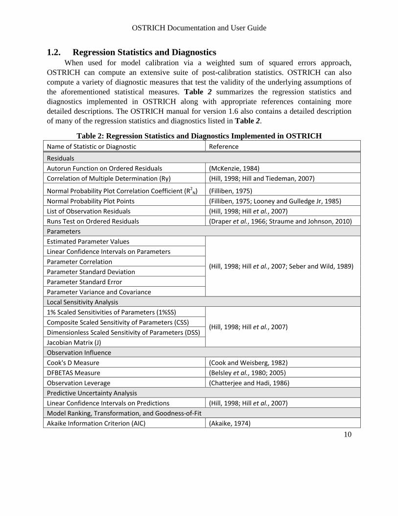
1.2. Regression Statistics and Diagnostics When used for model calibration via a weighted sum of squared errors approach,
OSTRICH can compute an extensive suite of post-calibration statistics. OSTRICH can also compute a variety of diagnostic measures that test the validity of the underlying assumptions of the aforementioned statistical measures. Table 2 summarizes the regression statistics and diagnostics implemented in OSTRICH along with appropriate references containing more detailed descriptions. The OSTRICH manual for version 1.6 also contains a detailed description of many of the regression statistics and diagnostics listed in Table 2.
Table 2: Regression Statistics and Diagnostics Implemented in OSTRICH Name of Statistic or Diagnostic Reference
Residuals Autorun Function on Ordered Residuals (McKenzie, 1984) Correlation of Multiple Determination (Ry) (Hill, 1998; Hill and Tiedeman, 2007)
Normal Probability Plot Correlation Coefficient (R2N) (Filliben, 1975)
Normal Probability Plot Points (Filliben, 1975; Looney and Gulledge Jr, 1985) List of Observation Residuals (Hill, 1998; Hill et al., 2007) Runs Test on Ordered Residuals (Draper et al., 1966; Straume and Johnson, 2010) Parameters Estimated Parameter Values
(Hill, 1998; Hill et al., 2007; Seber and Wild, 1989)
Linear Confidence Intervals on Parameters Parameter Correlation Parameter Standard Deviation Parameter Standard Error Parameter Variance and Covariance Local Sensitivity Analysis 1% Scaled Sensitivities of Parameters (1%SS)
(Hill, 1998; Hill et al., 2007) Composite Scaled Sensitivity of Parameters (CSS) Dimensionless Scaled Sensitivity of Parameters (DSS) Jacobian Matrix (J) Observation Influence Cook's D Measure (Cook and Weisberg, 1982) DFBETAS Measure (Belsley et al., 1980; 2005) Observation Leverage (Chatterjee and Hadi, 1986) Predictive Uncertainty Analysis Linear Confidence Intervals on Predictions (Hill, 1998; Hill et al., 2007) Model Ranking, Transformation, and Goodness-of-Fit Akaike Information Criterion (AIC) (Akaike, 1974)

OSTRICH Documentation and User Guide
11
Name of Statistic or Diagnostic Reference Bayesian Information Criterion (BIC) (Schwarz, 1978) Corrected Akaike Information Criterion (AICc) (Hurvich and Tsai, 1994; 1993) Estimated Box-Cox Transformation (Carroll and Ruppert, 1988; Sakia, 1992) Hannon-Quinn Information Criterion (HQ) (Hannan and Quinn, 1979) Standard Error (s)
(Hill, 1998; Hill et al., 2007; Seber et al., 1989) Variance (s2) Tests of the Linearity Assumption Beale's Linearity Measure (Beale, 1968) Linssen's Linearity Measure (Linssen, 1975)
2. ostIn.txt – the OSTRICH Input File This section summarizes the input file of the OSTRICH program. On case-sensitive Linux
systems, the input file must be named ostIn.txt. On Windows systems the file could also be named OstIn.txt. OSTRICH is a command-line console driven tool and when launched it will look for ostIn.txt in the working directory (i.e. the directory from which OSTRICH is launched). If this file does not exist or if it contains syntax errors, OSTRICH will quickly recognize this and report an error message and close. Windows users will experience this behavior as a brief flash of the DOS console window as it opens and then rapidly closes. In fact, the open-close sequence may happen so fast that all a user notices is a brief flicker on the computer monitor. This does not mean that OSTRICH is not installed correctly! It just means that you didn’t create a valid input file prior to running OSTRICH. The output file named “OstErrors0.txt” will have details on why OSTRICH failed to run.
For OSTRICH to work with a given modeling program, the modeling program must meet the following requirements:
• The modeling program must use a text-based input/output file format. OSTRICH can also work with modeling programs that use the MS Access or NetCDF file formats, but users will need to configure an additional section of the OSTRICH input file. This section is described in Section 2.17 (Type Conversions).
• The modeling program must be able to run without prompting for user intervention. This means, for example, that the modeling program cannot prompt the user to enter the name of an input file and the modeling program must not pause for user input at the end of a simulation.
• The output of the modeling program must be in a consistent format that can be reliably parsed. OSTRICH can also work with modeling programs that sometimes fail to write consistently formatted output. In such cases users should configure the optional “OnObsError” feature described in Section 2.3 (Basic Configuration).
OSTRICH Documentation and User Guide
12
OSTRICH utilizes a text-based input file format which specifies that configuration variables be organized on a line-by-line basis using loosely human-readable syntax. Users typically prepare the OSTRICH input file using a text editor like Notepad, Wordpad, VIM, or Emacs. For some sections (e.g. observations and response variables) it may also be helpful to use a spreadsheet program like Excel or Calc and then copy the desired cells from the spreadsheet to the text-based input file.
With a few exceptions (which will be explicitly noted in the following text) the basic format for a line of input in the ostIn.txt file is:
<variable> <value>
Where <variable> is the name of the configuration variable (e.g. ProgramType) and <value> is the user-selected value for the variable (e.g. ParticleSwarm). The whitespace separating <variable> and <value> can be any number of spaces or tab characters. Inside ostIn.txt, the OSTRICH configuration variables are organized into groups and each group is described below in its own section.
Although the list of ostIn.txt configuration groups is rather extensive, most of the groups do not need to be specified, as they are initialized within OSTRICH to reasonable defaults if the user does not set a value for them. Furthermore, many of the configuration groups relate to optional features within OSTRICH and may not be used in a given run of the program. In fact, the only groups that must be configured by the user are: Basic Configuration, File Pairs, and Parameters. You must also include an Observations group if calibrating using OSTRICH’s internal weighted least squares objective function. Otherwise, if using OSTRICH’s general-purpose constrained optimization platform (GCOP), you must include a Response Variables group, a Costs group, and a Constraints group. Sections 2.3 through 2.24 discuss the particular syntax and purpose of the various groups that may be included in the ostIn.txt file.
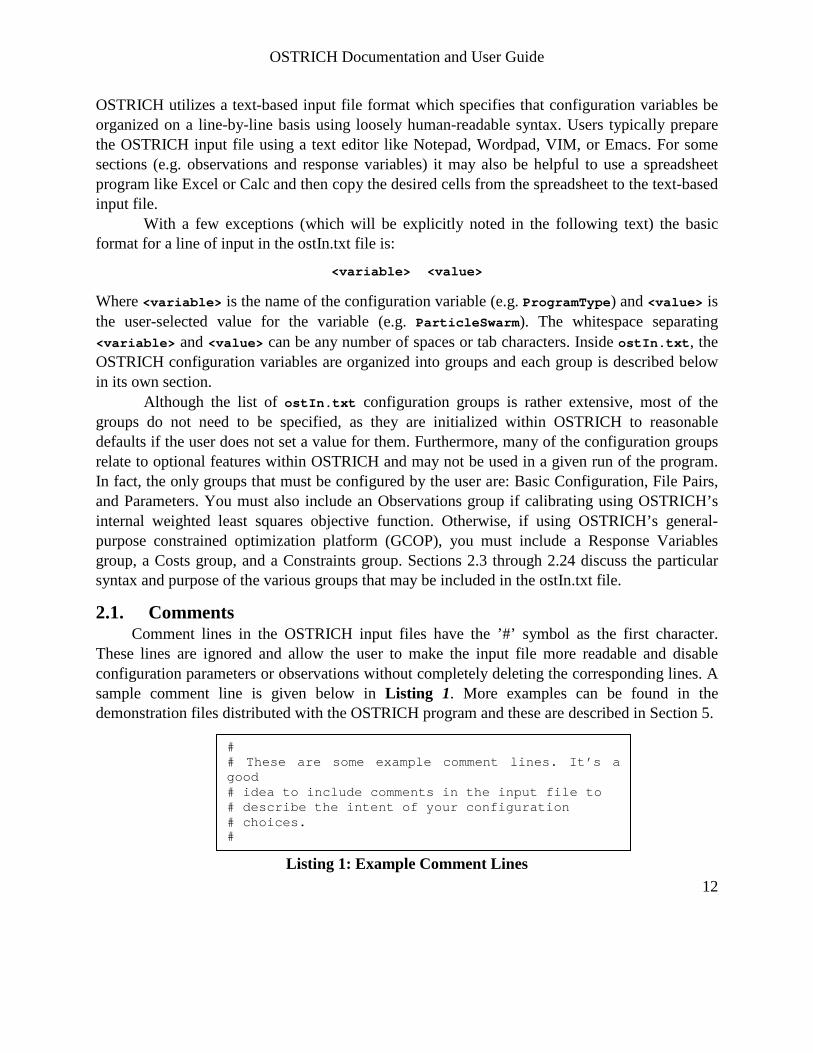
2.1. Comments Comment lines in the OSTRICH input files have the ’#’ symbol as the first character.
These lines are ignored and allow the user to make the input file more readable and disable configuration parameters or observations without completely deleting the corresponding lines. A sample comment line is given below in Listing 1. More examples can be found in the demonstration files distributed with the OSTRICH program and these are described in Section 5.
Listing 1: Example Comment Lines
# # These are some example comment lines. It’s a good # idea to include comments in the input file to # describe the intent of your configuration # choices. #
OSTRICH Documentation and User Guide
13
2.2. Case Sensitivity Variable names and group tags in the OSTRICH input file are case sensitive; e.g. using
beginfilepairs instead of BeginFilePairs will result in a parsing error. Meanwhile, values of variables are case insensitive; e.g. GENETICALGORITHM, geneticalgorithm, and GeneticAlgorithm will all correctly select the genetic algorithm ProgramType.
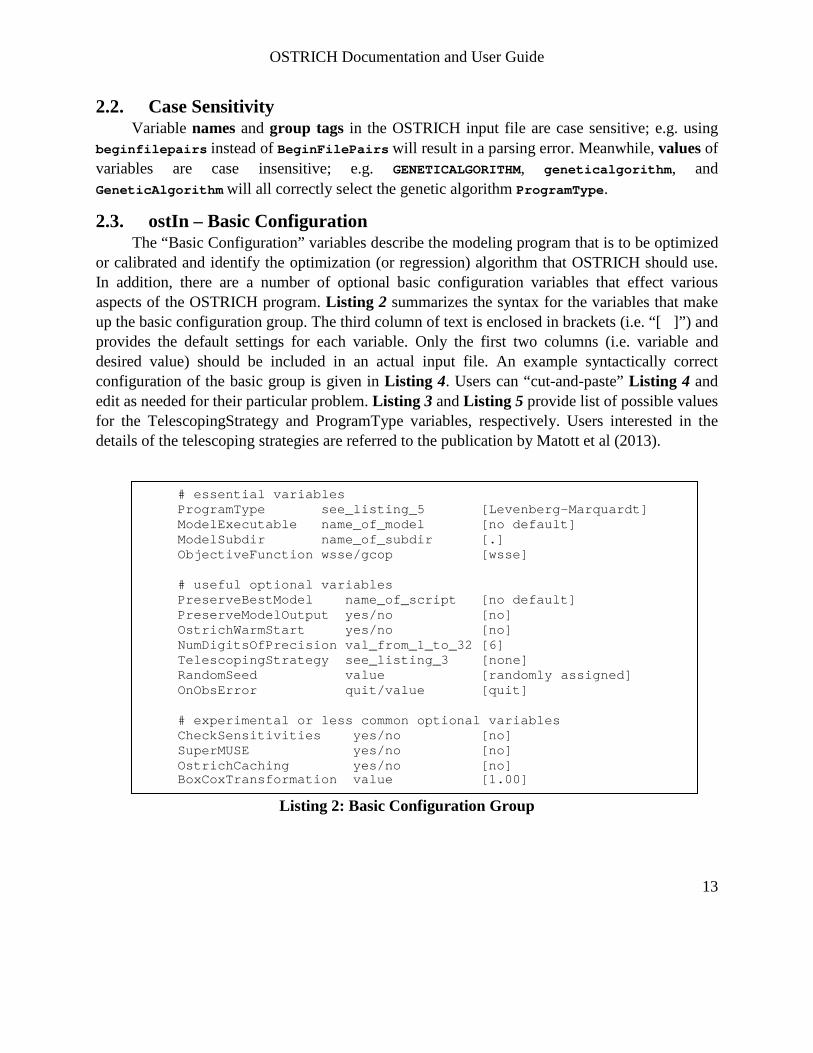
2.3. ostIn – Basic Configuration The “Basic Configuration” variables describe the modeling program that is to be optimized
or calibrated and identify the optimization (or regression) algorithm that OSTRICH should use. In addition, there are a number of optional basic configuration variables that effect various aspects of the OSTRICH program. Listing 2 summarizes the syntax for the variables that make up the basic configuration group. The third column of text is enclosed in brackets (i.e. “[ ]”) and provides the default settings for each variable. Only the first two columns (i.e. variable and desired value) should be included in an actual input file. An example syntactically correct configuration of the basic group is given in Listing 4. Users can “cut-and-paste” Listing 4 and edit as needed for their particular problem. Listing 3 and Listing 5 provide list of possible values for the TelescopingStrategy and ProgramType variables, respectively. Users interested in the details of the telescoping strategies are referred to the publication by Matott et al (2013).
Listing 2: Basic Configuration Group
# essential variables ProgramType see_listing_5 [Levenberg-Marquardt] ModelExecutable name_of_model [no default] ModelSubdir name_of_subdir [.] ObjectiveFunction wsse/gcop [wsse] # useful optional variables PreserveBestModel name_of_script [no default] PreserveModelOutput yes/no [no] OstrichWarmStart yes/no [no] NumDigitsOfPrecision val_from_1_to_32 [6] TelescopingStrategy see_listing_3 [none] RandomSeed value [randomly assigned] OnObsError quit/value [quit] # experimental or less common optional variables CheckSensitivities yes/no [no] SuperMUSE yes/no [no] OstrichCaching yes/no [no] BoxCoxTransformation value [1.00]
OSTRICH Documentation and User Guide
14
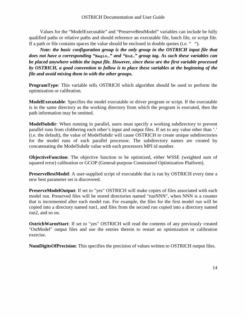
Values for the “ModelExecutable” and “PreserveBestModel” variables can include be fully qualified paths or relative paths and should reference an executable file, batch file, or script file. If a path or file contains spaces the value should be enclosed in double quotes (i.e. “ “).
Note: the basic configuration group is the only group in the OSTRICH input file that does not have a corresponding “Begin…” and “End…” group tag. As such these variables can be placed anywhere within the input file. However, since these are the first variable processed by OSTRICH, a good convention to follow is to place these variables at the beginning of the file and avoid mixing them in with the other groups. ProgramType: This variable tells OSTRICH which algorithm should be used to perform the optimization or calibration. ModelExecutable: Specifies the model executable or driver program or script. If the executable is in the same directory as the working directory from which the program is executed, then the path information may be omitted. ModelSubdir: When running in parallel, users must specify a working subdirectory to prevent parallel runs from clobbering each other’s input and output files. If set to any value other than ’.’ (i.e. the default), the value of ModelSubdir will cause OSTRICH to create unique subdirectories for the model runs of each parallel processor. The subdirectory names are created by concatenating the ModelSubdir value with each processors MPI id number. ObjectiveFunction: The objective function to be optimized, either WSSE (weighted sum of squared error) calibration or GCOP (General-purpose Constrained Optimization Platform). PreserveBestModel: A user-supplied script of executable that is run by OSTRICH every time a new best parameter set is discovered. PreserveModelOutput: If set to "yes" OSTRICH will make copies of files associated with each model run. Preserved files will be stored directories named "runNNN", when NNN is a counter that is incremented after each model run. For example, the files for the first model run will be copied into a directory named run1, and files from the second run copied into a directory named run2, and so on. OstrichWarmStart: If set to "yes" OSTRICH will read the contents of any previously created "OstModel" output files and use the entries therein to restart an optimization or calibration exercise. NumDigitsOfPrecision: This specifies the precision of values written to OSTRICH output files.

OSTRICH Documentation and User Guide
15
TelescopingStrategy: If selected, this optional setting will cause parameter bounds to become incrasingly smaller as an optimization or calibration proceeds.
Listing 3: Supported Values for the Telescoping Strategy Option
RandomSeed: This variable can be used to control the random seed OSTRICH uses when generating random numbers. OnObsError: This variable controls how OSTRICH behaves when a model fails to generate all of the expected output for a WSSE calibration. If set to "quit", OSTRICH will abort if it ever fails to parse an observation from user-specified output files. If set to a value, OSTRICH will use the value as a placeholder observation value if it can't read a given observation from model output. CheckSensitivities: If this variable is set to "yes", OSTRICH will perform a pre-calibration step to calculate parameter sensitivities (i.e. changes in simulated equivalent observations with respect to changes in parameters). SuperMUSE: If set to "yes", OSTRICH will interface with EPA SuperMUSE tasker-client approach to parallel computing. OstrichCaching: If set to "yes", OSTRICh will examine "OstModel" output files prior to running a given model configuration to see if the associated parameter set has already been evaluated. BoxCoxTransformation: If set to a value other than "1", OSTRICH will apply a Box-Cox power transformation on each calibration residual. The user-supplied value is used as the exponent for the transformation.
# Options for TelescopingStrategy # =========================================================== #none #convex-power #convex #linear #concave #delayed-concave

OSTRICH Documentation and User Guide
16
Listing 4: Example of a Syntactically Correct Basic Configuration Group
(note: variables set to default values could be omitted or commented out)
# essential variables ProgramType ParticleSwarm ModelExecutable “C:\My Folder\My_Model.exe” ModelSubdir mod ObjectiveFunction GCOP # useful optional variables PreserveBestModel “C:\My Folder\Save_Best.bat” PreserveModelOutput no OstrichWarmStart yes NumDigitsOfPrecision 8 TelescopingStrategy none RandomSeed 100 OnObsError quit # experimental or less common optional variables CheckSensitivities yes SuperMUSE no OstrichCaching no BoxCoxTransformation 1.00
OSTRICH Documentation and User Guide
17
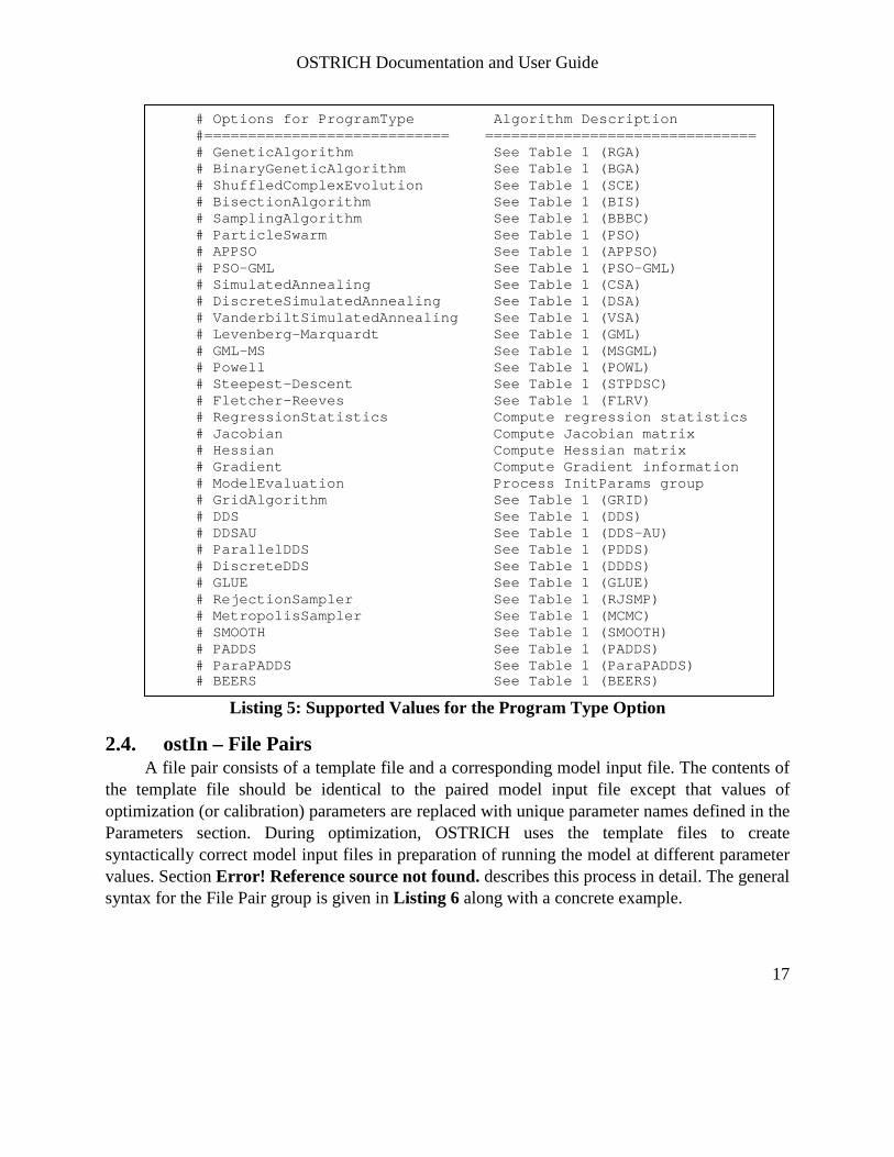
Listing 5: Supported Values for the Program Type Option
2.4. ostIn – File Pairs A file pair consists of a template file and a corresponding model input file. The contents of
the template file should be identical to the paired model input file except that values of optimization (or calibration) parameters are replaced with unique parameter names defined in the Parameters section. During optimization, OSTRICH uses the template files to create syntactically correct model input files in preparation of running the model at different parameter values. Section Error! Reference source not found. describes this process in detail. The general syntax for the File Pair group is given in Listing 6 along with a concrete example.
# Options for ProgramType Algorithm Description #============================ =============================== # GeneticAlgorithm See Table 1 (RGA) # BinaryGeneticAlgorithm See Table 1 (BGA) # ShuffledComplexEvolution See Table 1 (SCE) # BisectionAlgorithm See Table 1 (BIS) # SamplingAlgorithm See Table 1 (BBBC) # ParticleSwarm See Table 1 (PSO) # APPSO See Table 1 (APPSO) # PSO-GML See Table 1 (PSO-GML) # SimulatedAnnealing See Table 1 (CSA) # DiscreteSimulatedAnnealing See Table 1 (DSA) # VanderbiltSimulatedAnnealing See Table 1 (VSA) # Levenberg-Marquardt See Table 1 (GML) # GML-MS See Table 1 (MSGML) # Powell See Table 1 (POWL) # Steepest-Descent See Table 1 (STPDSC) # Fletcher-Reeves See Table 1 (FLRV) # RegressionStatistics Compute regression statistics # Jacobian Compute Jacobian matrix # Hessian Compute Hessian matrix # Gradient Compute Gradient information # ModelEvaluation Process InitParams group # GridAlgorithm See Table 1 (GRID) # DDS See Table 1 (DDS) # DDSAU See Table 1 (DDS-AU) # ParallelDDS See Table 1 (PDDS) # DiscreteDDS See Table 1 (DDDS) # GLUE See Table 1 (GLUE) # RejectionSampler See Table 1 (RJSMP) # MetropolisSampler See Table 1 (MCMC) # SMOOTH See Table 1 (SMOOTH) # PADDS See Table 1 (PADDS) # ParaPADDS See Table 1 (ParaPADDS) # BEERS See Table 1 (BEERS)
OSTRICH Documentation and User Guide
18
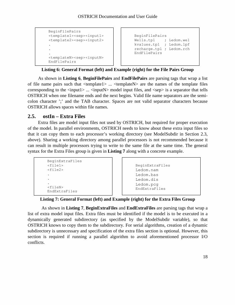
Listing 6: General Format (left) and Example (right) for the File Pairs Group
As shown in Listing 6, BeginFilePairs and EndFilePairs are parsing tags that wrap a list of file name pairs such that <template1> ... <templateN> are the names of the template files corresponding to the <input1> ... <inputN> model input files, and <sep> is a separator that tells OSTRICH when one filename ends and the next begins. Valid file name separators are the semi-colon character ’;’ and the TAB character. Spaces are not valid separator characters because OSTRICH allows spaces within file names.
2.5. ostIn – Extra Files Extra files are model input files not used by OSTRICH, but required for proper execution
of the model. In parallel environments, OSTRICH needs to know about these extra input files so that it can copy them to each processor’s working directory (see ModelSubdir in Section 2.3, above). Sharing a working directory among parallel processors is not recommended because it can result in multiple processors trying to write to the same file at the same time. The general syntax for the Extra Files group is given in Listing 7 along with a concrete example.
Listing 7: General Format (left) and Example (right) for the Extra Files Group
As shown in Listing 7, BeginExtraFiles and EndExtraFiles are parsing tags that wrap a list of extra model input files. Extra files must be identified if the model is to be executed in a dynamically generated subdirectory (as specified by the ModelSubdir variable), so that OSTRICH knows to copy them to the subdirectory. For serial algorithms, creation of a dynamic subdirectory is unnecessary and specification of the extra files section is optional. However, this section is required if running a parallel algorithm to avoid aforementioned processor I/O conflicts.
BeginFilePairs <template1><sep><input1> <template2><sep><input2> . . . <templateN><sep><inputN> EndFilePairs
BeginFilePairs Wells.tpl ; Ledom.wel kvalues.tpl ; Ledom.lpf recharge.tpl ; Ledom.rch EndFilePairs
BeginExtraFiles <file1> <file2> . . . <fileN> EndExtraFiles
BeginExtraFiles Ledom.nam Ledom.bas Ledom.dis Ledom.pcg EndExtraFiles
OSTRICH Documentation and User Guide
19
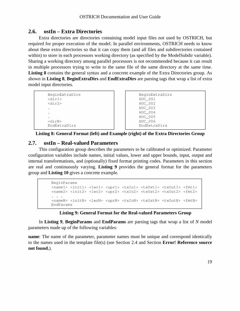
2.6. ostIn – Extra Directories Extra directories are directories containing model input files not used by OSTRICH, but
required for proper execution of the model. In parallel environments, OSTRICH needs to know about these extra directories so that it can copy them (and all files and subdirectories contained within) to store in each processors working directory (as specified by the ModelSubdir variable). Sharing a working directory among parallel processors is not recommended because it can result in multiple processors trying to write to the same file of the same directory at the same time. Listing 8 contains the general syntax and a concrete example of the Extra Directories group. As shown in Listing 8, BeginExtraDirs and EndExtraDirs are parsing tags that wrap a list of extra model input directories.
Listing 8: General Format (left) and Example (right) of the Extra Directories Group
2.7. ostIn – Real-valued Parameters This configuration group describes the parameters to be calibrated or optimized. Parameter
configuration variables include names, initial values, lower and upper bounds, input, output and internal transformations, and (optionally) fixed format printing codes. Parameters in this section are real and continuously varying. Listing 9 provides the general format for the parameters group and Listing 10 gives a concrete example.
Listing 9: General Format for the Real-valued Parameters Group
In Listing 9, BeginParams and EndParams are parsing tags that wrap a list of N model parameters made up of the following variables:
name: The name of the parameter, parameter names must be unique and correspond identically to the names used in the template file(s) (see Section 2.4 and Section Error! Reference source not found.).
BeginExtraDirs <dir1> <dir2> . . . <dirN> EndExtraDirs
BeginExtraDirs HUC_001 HUC_002 HUC_003 HUC_004 HUC_005 HUC_006 EndExtraDirs
BeginParams <name1> <init1> <lwr1> <upr1> <txIn1> <txOst1> <txOut1> <fmt1> <name2> <init2> <lwr2> <upr2> <txIn2> <txOst2> <txOut2> <fmt2> . . . <nameN> <initN> <lwrN> <uprN> <txInN> <txOstN> <txOutN> <fmtN> EndParams
OSTRICH Documentation and User Guide
20
init: Initial value of the parameter, in units specified by the txIn variable. Alternatively, the keywords “random” or “extract” may be used instead of specifying a value. OSTRICH will assign a randomly generated initial value if the “random” keyword is used. OSTRICH will extract the initial value from existing model input files if the “extract” keyword is used.
lwr: Lower bound (i.e. minimum value) of the parameter, in units specified by the txIn variable.
upr: Upper bound (i.e.. maximum value) of the parameter, in units specified by the txIn variable.
txIn, txOst, and txOut: These specify the type of transformation units that OSTRICH should use. Transformations allow the user to take advantage of any linearity relationships that exist between a transformed parameter value (e.g. log10 or loge) and the underlying model. Three kinds of transformations are provided so that the user can work with input and output transformations that are different than the internal transformation. Typically, the user will request no input and output transformation (so that input and output values are the native units of the parameter), while instructing OSTRICH to perform a transformation internally. This approach allows the algorithm to take advantage of a transformed relationship without requiring manual conversion of input and output values. However, it should be noted that some statistical output is reported in terms of txOst units, regardless of the value of txOut; namely (a) parameter variance-covariance, (b) observation influence, (c)parameter sensitivity, (d) model linearity, and (e) matrices. OSTRICH supports the following transformation values:
– none: no transformation.
– log10: log base 10 transformation.
– ln: natural logarithm transformation.
fmt: A format code that OSTRICH will use when writing model input files. This is provided so that OSTRICH can support modeling programs which expect fixed format inputs (i.e. when values in the input file are expected to take up an exact number of characters). For example, many programs written in legacy FORTRAN (e.g. F77) expect fixed format. Use a fmt value of “free” if using a modeling program that is not bound by fixed format requirements. Otherwise, use a format code of “Fw.d” for decimal values (e.g. 3.4567) where “w” is the total number of characters and “d” is the number of characters following the decimal. For example, to represent the value of Pi to 6 significant digits you would use a format code of F8.6, resulting in a value of “3.141593”. Use a format code of “Ew.d” or “Dw.d” for scientific notation, where “w” is the total number of characters and “d” is the number of significant digits. For example, applying a format code of E10.3 to the value of 1/12 would result in “ 8.333E-02”. For fixed decimal notation “w” should be at least equal to “d”+2 and for fixed scientific notation “w” should be at least equal to “d”+7.

OSTRICH Documentation and User Guide
21
Listing 10: Example of the Real-valued Parameters Group
2.8. ostIn – Integer Parameters This configuration group describes those parameters to be calibrated or optimized which
can take on only integer values. Like their real-parameter counterparts, integer parameter configuration variables include names, initial values, and lower and upper bounds. However, format codes and unit transformations are not supported for integer parameters. Listing 11 provides the general syntax and a concrete example of the integer parameters group.
Listing 11: General Format (left) and Example (right) for the Integer Parameters Group
2.9. ostIn – Combinatorial Parameters This configuration group describes those parameters to be calibrated or optimized which
can take on a discrete set of values, which can be in the form of real, integer or string (text) values. Like integer and real parameters, combinatorial parameter configuration variables include names and initial values; but instead of lower and upper bounds, the user must supply a complete list of the discrete values that may be assigned to the parameter. Furthermore, format codes and unit transformations are not supported for combinatorial parameters. Listing 12 provides the general syntax of the combinatorial parameters group.
Listing 12: General Format for the Combinatorial Parameters Group
In Listing 12, the “type” field should be either “real”, “integer”, or “string” and should correspond to the type of values in the subsequent combinatorial list. Furthermore, the “N1” through “NM” values specify the number of entries in the combinatorial list, which is generically represented in Listing 12 as vm,n for the nth discrete value that can be taken on by the mth parameter. Listing 13 provides a concrete example of the combinatorial parameters group.
BeginParams _DIAM_ random 10.0 50.0 none none none free _LEN_ random 200.0 1000.0 none none none free EndParams
BeginIntegerParams <name1> <init1> <lwr1> <upr1> <name2> <init2> <lwr2> <upr2> . . . <nameN> <initN> <lwrN> <uprN> EndIntegerParams
BeginIntegerParams N_INJ_WELLS 2 0 20 N_EXT_WELLS 6 0 50 EndIntegerParams
BeginCombinatorialParams <name1> <type1> <init1> <N1> <v1,1> <v1,2> ... <v1,N1> <name2> <type2> <init2> <N2> <v2,1> <v2,2> ... <v2,N2> . . . <nameM> <typeM> <initM> <NM> <vM,1> <vM,2> ... <vM,NM> EndCombinatorialParams
OSTRICH Documentation and User Guide
22
Listing 13: Example of the Combinatorial Parameters Group
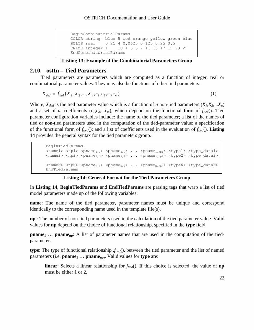
2.10. ostIn – Tied Parameters Tied parameters are parameters which are computed as a function of integer, real or
combinatorial parameter values. They may also be functions of other tied parameters.
),...,,,,...,,( 2121 mntiedtied cccXXXfX = (1)
Where, Xtied is the tied parameter value which is a function of n non-tied parameters (X1,X2,...Xn) and a set of m coefficients (c1,c2,...cm), which depend on the functional form of ftied(). Tied parameter configuration variables include: the name of the tied parameter; a list of the names of tied or non-tied parameters used in the computation of the tied-parameter value; a specification of the functional form of ftied(); and a list of coefficients used in the evaluation of ftied(). Listing 14 provides the general syntax for the tied parameters group.
Listing 14: General Format for the Tied Parameters Group
In Listing 14, BeginTiedParams and EndTiedParams are parsing tags that wrap a list of tied model parameters made up of the following variables:
name: The name of the tied parameter, parameter names must be unique and correspond identically to the corresponding name used in the template file(s).
np : The number of non-tied parameters used in the calculation of the tied parameter value. Valid values for np depend on the choice of functional relationship, specified in the type field.
pname1 … pnamenp: A list of parameter names that are used in the computation of the tied-parameter.
type: The type of functional relationship ,ftied(), between the tied parameter and the list of named parameters (i.e. pname1 … pnamenp). Valid values for type are:
linear: Selects a linear relationship for ftied(). If this choice is selected, the value of np must be either 1 or 2.
BeginCombinatorialParams COLOR string blue 5 red orange yellow green blue BOLTS real 0.25 4 0.0625 0.125 0.25 0.5 PRIME integer 1 10 1 3 5 7 11 13 17 19 23 29 EndCombinatorialParams
BeginTiedParams <name1> <np1> <pname1,1> <pname1,2> ... <pname1,np1> <type1> <type_data1> <name2> <np2> <pname2,1> <pname2,2> ... <pname2,np2> <type2> <type_data2> . . . <nameN> <npN> <pnameN,1> <pnameN,2> ... <pnameN,npN> <typeN> <type_dataN> EndTiedParams
OSTRICH Documentation and User Guide
23
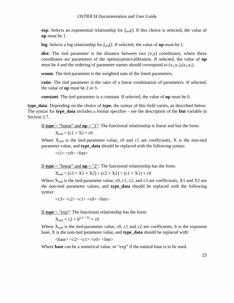
exp: Selects an exponential relationship for ftied(). If this choice is selected, the value of np must be 1.
log: Selects a log relationship for ftied(). If selected, the value of np must be 1.
dist: The tied parameter is the distance between two (x,y) coordinates, where these coordinates are parameters of the optimization/calibration. If selected, the value of np must be 4 and the ordering of parameter names should correspond to (x1,y1),(x2,y2).
wsum: The tied parameter is the weighted sum of the listed parameters.
ratio: The tied parameter is the ratio of a linear combination of parameters. If selected, the value of np must be 2 or 3.
constant: The tied parameter is a constant. If selected, the value of np must be 0.
type_data: Depending on the choice of type, the syntax of this field varies, as described below. The syntax for type_data includes a format specifier – see the description of the fmt variable in Section 2.7.
If type = ”linear” and np = "1": The functional relationship is linear and has the form: Xtied = (c1 × X) + c0
Where Xtied is the tied-parameter value, c0 and c1 are coefficients, X is the non-tied parameter value, and type_data should be replaced with the following syntax:
<c1> <c0> <fmt> If type = ”linear” and np = "2": The functional relationship has the form:
Xtied = (c3 × X1 × X2) + (c2 × X2) + (c1 × X1) + c0 Where Xtied is the tied-parameter value, c0, c1, c2, and c3 are coefficients, X1 and X2 are the non-tied parameter values, and type_data should be replaced with the following syntax:
<c3> <c2> <c1> <c0> <fmt> If type = ”exp”: The functional relationship has the form:
Xtied = c2 × b(c1 × X) + c0 Where Xtied is the tied-parameter value, c0, c1 and c2 are coefficients, b is the exponent base, X is the non-tied parameter value, and type_data should be replaced with:
<base> <c2> <c1> <c0> <fmt> Where base can be a numerical value, or “exp” if the natural base is to be used.

OSTRICH Documentation and User Guide
24
If type = ”log”: The functional relationship has the form: Xtied = c3 × loga(c2 × X + c1) + c0
Where Xtied is the tied-parameter value, c0, c1, c2 and c3 are coefficients, a is the logarithm base, X is the non-tied parameter, and type_data should be replaced with the following syntax:
<base> <c3> <c2> <c1> <c0> <fmt> Where base can be a numerical value, or “ln” if the natural logarithm is to be used.
If type = ”dist”: The type_data field should contain the desired fmt specification.
If type = ”wsum”: The type_data field should list the values of each weight, using the same ordering as the named list of parameters, followed by the desired fmt specification.
If type = ”ratio” and np = “2”: The functional relationship has the form:
Xtied = (c3 × X1 + c2) / (c1 × X2 + c0)
Where Xtied is the tied-parameter value, c3, c2, c1 and c0 are coefficients, X1 and X2 are non-tied parameters, and type_data should be replaced with the following syntax:
<c3> <c2> <c1> <c0> <fmt> If type = ”ratio” and np = “3”: The functional relationship has the form:
Xtied = [ (n7 × X1 × X2 × X3) + (n6 × X1 × X2) + (n5 × X1 × X3) + (n4 × X2 × X3) + (n3 × X1) + (n2 × X2) + (n1 × X3) + n0 ] / [ (d7× X1 × X2 × X3) + (d6 × X1 × X2) + (d5 × X1 × X3) + (d4 × X2 × X3) + (d3 × X1) + (d2 × X2) + (d1 × X3) + d0 ]
Where Xtied is the tied-parameter value, n7 … n0 and d7 … d0 are coefficients, X1 … X3 are non-tied parameters, and type_data should be replaced with the following syntax:
n7 n6 n5 n4 n3 n2 n1 n0 d7 d6 d5 d4 d3 d2 d1 d0 fmt
If np = “0”: The tied parameter is assigned a constant value. No type field is required and the type_data field must contain the parameter value followed by a format specifier (fmt).
Listing 15 provides concrete examples of the different tied parameter types.

OSTRICH Documentation and User Guide
25
Listing 15: Example of the Tied Parameters Group
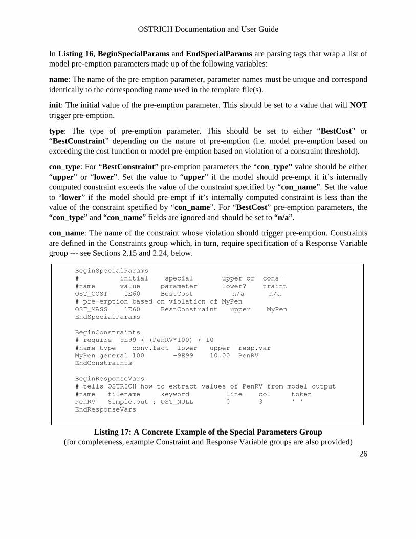
2.11. ostIn – Special Parameters (pre-emption) Certain models are capable of monitoring the progress of a simulation and aborting further
processing if some threshold cost or constraint is exceeded. OSTRICH provides the “SpecialParams” group to support such models. Special parameters are cost and constraint thresholds that are tracked by selected algorithms in OSTRICH (see the relevant column in Table 1, above) and written to input files using the same template mechanism as regular calibration/optimization parameters. In this way OSTRICH can pass the most up to date threshold values on to the pre-emptive model. Pre-emption is described in detail by Razavi et al (2010). The general syntax for the SpecialParams group is given below in Listing 16 and a concrete example is given in Listing 17.
Listing 16: General Format of the Special Parameters Group
BeginTiedParams # 1-parameter linear (TLIN = 2*XVAL) TLIN 1 XVAL linear 2.00 0.00 free # 2-parameter linear (TLN2 = 2*XVAL + YVAL) TLN2 2 XVAL YVAL linear 0.00 2.00 1.00 0.00 free # exponent, base e (TEXP = exp(-XVAL)) TEXP 1 XVAL exp exp 1.00 -1.00 0.00 free # exponent, base 10 (TX2P = 10^(-XVAL)) TXP2 1 XVAL exp 10.0 1.00 -1.00 0.00 free # logarithm, natural log (TLOG = 2*LN(XVAL)) TLOG 1 XVAL log ln 2.00 -1.00 0.00 0.00 free # logarithm, base 2 (TLG2 = log2(XVAL/2)+1) TLG2 1 XVAL log 2.00 1.00 0.50 0.00 1.00 free # distance TDST 4 X1VAL Y1VAL X2VAL Y2VAL dist free # weighted sum (TSUM = (1/3)*(XVAL+YVAL+ZVAL)) TSUM 3 XVAL YVAL ZVAL wsum 0.33 0.33 0.33 free # 2-parameter ratio (TRAT = (XVAL / YVAL)) TRAT 2 XVAL YVAL ratio 1.00 0.00 1.00 0.00 free # 3-parameter ratio (TRT3 = (XVAL*YVAL)/(ZVAL+1)) TRT3 3 XVAL YVAL ZVAL ratio 0 1 0 0 0 0 0 0 0 0 0 0 0 0 1 1 free # constant (Pi) TPI 0 3.1415 free EndTiedParams
BeginSpecialParams <name1> <init1> <type1> <con_type1> <con_name1> <name1> <init1> <type1> <con_type1> <con_name1> . . . <name1> <init1> <type1> <con_type1> <con_name1> EndSpecialParams
OSTRICH Documentation and User Guide
26
In Listing 16, BeginSpecialParams and EndSpecialParams are parsing tags that wrap a list of model pre-emption parameters made up of the following variables:
name: The name of the pre-emption parameter, parameter names must be unique and correspond identically to the corresponding name used in the template file(s).
init: The initial value of the pre-emption parameter. This should be set to a value that will NOT trigger pre-emption.
type: The type of pre-emption parameter. This should be set to either “BestCost” or “BestConstraint” depending on the nature of pre-emption (i.e. model pre-emption based on exceeding the cost function or model pre-emption based on violation of a constraint threshold).
con_type: For “BestConstraint” pre-emption parameters the “con_type” value should be either “upper” or “lower”. Set the value to “upper” if the model should pre-empt if it’s internally computed constraint exceeds the value of the constraint specified by “con_name”. Set the value to “lower” if the model should pre-empt if it’s internally computed constraint is less than the value of the constraint specified by “con_name”. For “BestCost” pre-emption parameters, the “con_type” and “con_name” fields are ignored and should be set to “n/a”.
con_name: The name of the constraint whose violation should trigger pre-emption. Constraints are defined in the Constraints group which, in turn, require specification of a Response Variable group --- see Sections 2.15 and 2.24, below.
Listing 17: A Concrete Example of the Special Parameters Group
(for completeness, example Constraint and Response Variable groups are also provided)
BeginSpecialParams # initial special upper or cons- #name value parameter lower? traint OST_COST 1E60 BestCost n/a n/a # pre-emption based on violation of MyPen OST_MASS 1E60 BestConstraint upper MyPen EndSpecialParams BeginConstraints # require -9E99 < (PenRV*100) < 10 #name type conv.fact lower upper resp.var MyPen general 100 -9E99 10.00 PenRV EndConstraints BeginResponseVars # tells OSTRICH how to extract values of PenRV from model output #name filename keyword line col token PenRV Simple.out ; OST_NULL 0 3 ' ' EndResponseVars

OSTRICH Documentation and User Guide
27
2.12. ostIn – Initial Parameters As indicated in Table 1, users of certain algorithms can optionally seed some or all of the
initial search entries with predefined parameter sets. This allows the user to incorporate prior information (such as previous optimization results or expert judgement) into the optimization, and may enhance the efficiency and/or effectiveness of the algorithm. To use this option, insert an “InitParams” group, which uses the general syntax given in Listing 18.
Listing 18: General Format of the Initial Parameters Group
Where “BeginInitParams” and “EndInitParams” are parsing tags that wrap a list of initial parameters, and n is the number of parameters, m is the number of entries in the initial parameters group, and pi,j is the j-th initial value of the i-th parameter (ordered according to the order of the parameters section(s)). A concrete example of the “InitParams” group is given in Listing 19.
Listing 19: Example of the Initial Parameters Group
(with parameters group included for completeness)
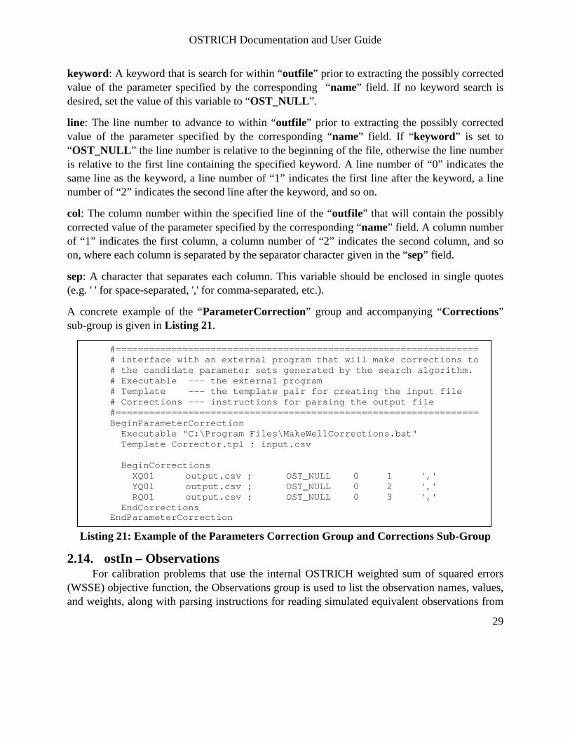
2.13. ostIn – Parameter Correction The “ParameterCorrection” group and corresponding “Corrections” sub-group allows
users to interface OSTRICH with an external program or script that makes adjustments to a candidate parameter set that has been calculated by an OSTRICH search algorithm but not yet evaluated. These corrections allows users to incorporate expert judgment or other information
BeginInitParams p1,1 p2,1 p3,1 . . . pn,1 p1,2 p2,2 p3,2 . . . pn,2 . . . . . . p1,m p2,m p3,m . . . pn,m EndInitParams
BeginParams xval 0 -20.0 +20.0 none none none yval 0 -20.0 +20.0 none none none zval 0 -20.0 +20.0 none none none EndParams BeginInitParams #xval yval zval 0.0 0.0 0.0 0.0 0.0 10.0 0.0 10.0 0.0 10.0 0.0 0.0 20.0 20.0 20.0 EndInitParams

OSTRICH Documentation and User Guide
28
into the search procedure while still using one of the algorithms already implemented within OSTRICH. As an example, consider an optimization problem that seeks to install a well in an optimal location for extracting contaminated groundwater. Parameter correction can be used to adjust candidate well locations if they are found to be outside the boundaries of the contaminated plume. To use this option, insert a “ParameterCorrection” group, which uses the general syntax given in Listing 20 and which includes a “Corrections” sub-group.
Listing 20: General Syntax for the Parameters Correction
Group and Corrections Sub-Group
Where “BeginParameterCorrection” and “EndParameterCorrection” are parsing tags that wrap the configuration variables of the “ParameterCorrection” group and “BeginCorrections” and “EndCorrections” are parsing tags that wrap the “Corrections” sub-group. Configuration variables are described below:
name_of_exe: The name (including path, if desired) of the external correction program or script that implements user-defined parameter corrections.
tpl_name: The name of the template file that mimics the input file used by the external parameter correction program (i.e. “name_of_exe”). The template file must contain the names of all parameters that are to be subjected to possible correction by the external program.
inp_name: The name of the input file read by the “name_of_exe” parameter. OSTRICH will create this file by replacing the parameter names listed in the “tpl_name” template file with actual candidate values under consideration by the search algorithm.
name: The name of a correctable parameter listed in the template file (i.e. “tpl_name”). Each correctable parameter must be included in the Corrections sub-group.
outfile: The name of the file that will be created by the external correction program and which will contain the possibly corrected value of the parameter specified by the corresponding “name” field.
BeginParameterCorrection Executable <name_of_exe> Template <tpl_name> ; <inp_name> BeginCorrections <name1> <outfile1> ; <keyword1> <line1> <col1> '<sep1>' <name2> <outfile2> ; <keyword2> <line2> <col2> '<sep2>' . . . <nameN> <outfileN> ; <keywordN> <lineN> <colN> '<sepN>' EndCorrections EndParameterCorrection
OSTRICH Documentation and User Guide
29
keyword: A keyword that is search for within “outfile” prior to extracting the possibly corrected value of the parameter specified by the corresponding “name” field. If no keyword search is desired, set the value of this variable to “OST_NULL”.
line: The line number to advance to within “outfile” prior to extracting the possibly corrected value of the parameter specified by the corresponding “name” field. If “keyword” is set to “OST_NULL” the line number is relative to the beginning of the file, otherwise the line number is relative to the first line containing the specified keyword. A line number of “0” indicates the same line as the keyword, a line number of “1” indicates the first line after the keyword, a line number of “2” indicates the second line after the keyword, and so on.
col: The column number within the specified line of the “outfile” that will contain the possibly corrected value of the parameter specified by the corresponding “name” field. A column number of “1” indicates the first column, a column number of “2” indicates the second column, and so on, where each column is separated by the separator character given in the “sep” field.
sep: A character that separates each column. This variable should be enclosed in single quotes (e.g. ' ' for space-separated, ',' for comma-separated, etc.).
A concrete example of the “ParameterCorrection” group and accompanying “Corrections” sub-group is given in Listing 21.
Listing 21: Example of the Parameters Correction Group and Corrections Sub-Group
2.14. ostIn – Observations For calibration problems that use the internal OSTRICH weighted sum of squared errors
(WSSE) objective function, the Observations group is used to list the observation names, values, and weights, along with parsing instructions for reading simulated equivalent observations from
#================================================================= # interface with an external program that will make corrections to # the candidate parameter sets generated by the search algorithm. # Executable --- the external program # Template --- the template pair for creating the input file # Corrections --- instructions for parsing the output file #================================================================= BeginParameterCorrection Executable "C:\Program Files\MakeWellCorrections.bat" Template Corrector.tpl ; input.csv BeginCorrections XQ01 output.csv ; OST_NULL 0 1 ',' YQ01 output.csv ; OST_NULL 0 2 ',' RQ01 output.csv ; OST_NULL 0 3 ',' EndCorrections EndParameterCorrection

OSTRICH Documentation and User Guide
30
model output files. The general syntax for the Observations group is given in Listing 22 and a concrete example is given in Listing 23.
Listing 22: General Format of the Observations Group
Listing 23: An Example of the Observations Group
In Listing 22 and Listing 23, BeginObservations and EndObservations are parsing tags that wrap a list of observations, which are made up of the following variables: name: The name of the observation, each observation should have a unique name.
value: The field-measured value of the observation.
wgt: The weight assigned to the observation. See Hill (1998) and Hill and Tiedeman (2007) for guidelines to assigning observation weights.
file: The model output file where the simulated value of the observation will be stored following execution of the modeling program.
sep: This variable is a filename separator (i.e. a tab or semi-colon). See also the File Pairs section (Section 2.4).
key, line, col, and, tok: These variables tell OSTRICH how to extract model simulated observation values from the model output file. First, OSTRICH positions the output file parser at the first line in file containing key(word). If OSTRICH should begin parsing at the beginning of the file, then the value of key should be OST_NULL. Next, the parser uses the line and col values to locate the position of the desired observation value. This value is then extracted and converted to a double precision number. The parsing process is repeated until all observation
BeginObservations <name1><value1><wgt1><file1><sep1><key1><line1><col1><tok1><aug1><grp1> <name2><value2><wgt2><file2><sep2><key2><line2><col2><tok2><aug2><grp2> . . . <nameN><valueN><wgtN><fileN><sepN><keyN><lineN><colN><tokN><augN><grpN> EndObservations
BeginObservations #name val wgt filenamee ; keyword line col tok aug? group MW1 68 1.00 headerr.dat ; computed 2 3 ' ' no mw MW2 70 1.00 headerr.dat ; computed 3 3 ' ' no mw MW3 65 1.00 headerr.dat ; computed 4 3 ' ' no mw EndObservations

OSTRICH Documentation and User Guide
31
values are read. The line variable tells OSTRICH how many lines must be skipped, starting from the line containing key, before the line containing the desired observation value is reached. Therefore, if the observation value is on the same line as key, then line should be equal to 0; if the observation value is on the line immediately following key, then line should be equal to 1, and so on. The col variable tells OSTRICH which column in the line contains the desired observation value; where column numbering begins at 1 and the tok variable specifies the column separator. Note that values for the tok variable should be enclosed in single quotes (e.g. ‘,’ for a comma token). Furthermore, providing a whitespace token (e.g. ‘ ‘) will cause any sequence of space or TAB characters to be treated as a single column separator token. Figure 1 illustrates the parse procedure using an example observation list (Listing 23) and model output file (Figure 2).
aug: Setting the value of the aug (i.e. augmented output) variable to yes will cause OSTRICH to include the simulated values of the selected observation(s) in the OstModel output file (see Section 4.5). This can be useful, for example, when assembling samples for a predictive uncertainty analysis.
grp: Use the grp variable to partition observations into meaningful groups (e.g. high- vs. low-flow observations, groundwater head vs. flow observations, nitrate vs. trichloroethylene concentrations, etc.). When performing multi-criteria calibration, OSTRICH will compute multiple WSSR objectives corresponding to each unique observation group.

OSTRICH Documentation and User Guide
32
Figure 1: General Parse Procedure for Extracting Simulated Equivalents
with Application to Example Output in Figure 2 using Instructions in Listing 23
Figure 2: Example Model Output for Illustrating Extraction of Simulated Equivalent Observations

OSTRICH Documentation and User Guide
33
2.15. ostIn – Response Variables When performing optimization (as opposed to calibration), this group specifies the
response variables that OSTRICH should read from model output files prior to evaluating costs and constraints. The syntax is very similar to the observations group used in model calibration, and includes variable name, output file name (from which the value of the variable is read), and parsing instructions for retrieving the value of the variable from the given model output file. The Constraints and GCOP sections (see below) build upon the Response and Tied Response Variable groups by associating response variables with a constraint or cost variable. The general syntax for the “ResponseVars” group is given in Listing 24 and a concrete example is given in Listing 25.
Listing 24: General Format of the ResponseVariable Group
Listing 25: An Example of the ResponseVariable Group
Where BeginResponseVars and EndResponseVars are parsing tags that wrap a list of response variables, which are made up of the following variables:
name: The name of the response variable, each should have a unique name.
file: The model output file where the simulated value of the response variable will be stored following execution of the modeling program.
sep: This variable is a filename separator (i.e. a tab or semi-colon). See also the File Pairs section (Section 2.4).
key, line, col, and tok: These variables tell OSTRICH how to extract model simulated response variable values from the model output file. The parsing procedure is identical to that used in extracting Observation group data (see Section 2.14 for details).
BeginResponseVars <name1><file1><sep1><key1><line1><col1><tok1><aug1> <name2><file2><sep2><key2><line2><col2><tok2><aug2> . . . <nameN><fileN><sepN><keyN><lineN><colN><tokN><augN> EndResponseVars
BeginResponseVars #name filename key line col token augmented? F1 CanBeam.out ; F1 0 2 '=' yes F2 CanBeam.out ; F2 1 2 '=' yes EndResponseVars

OSTRICH Documentation and User Guide
34
aug: Setting the value of the aug (i.e. augmented output) variable to yes will cause OSTRICH to include the simulated values of the selected response variable(s) in the OstModel output file (see Section 4.5). For multi-objective problems, there should be a one-to-one correspondence between cost functions (see Section 2.23) and augmented response variables.
2.16. ostIn – Tied Response Variables This group specifies ’tied’ response variables; variables whose values are computed by
OSTRICH as functions of one or more response variables and/or parameters. The general syntax for the “TiedRespVars” group is given in Listing 26 and a concrete example is given in Listing 27.
Listing 26: General Format of the Tied Response Variable Group
Listing 27: An Example of the Tied Response Variable Group
In Listing 26 and Listing 27, BeginTiedRespVars and EndTiedRespVars are parsing tags that wrap a list of tied response variables. The parameters in this section are identical to those in the Tied Parameters (see Section 2.10), except fewer functional relationships are supported and the list of non-tied items (used in the calculation of the tied response variable) may be parameters, response variables, and/or other tied response variables.
name: The name of the tied response variable, each should have a unique name.
np: The number of parameters, response variables and/or other tied response variables used in the calculation of the named tied response variable. Valid values for np depend on the choice of functional relationship, specified in the type field.
BeginTiedRespVars <name1> <np1> <pname1,1> <pname1,2> ... <pname1,np1> <type1> <type_data1> <name2> <np2> <pname2,1> <pname2,2> ... <pname2,np2> <type2> <type_data2> . . . <nameN> <npN> <pnameN,1> <pnameN,2> ... <pnameN,npN> <typeN> <type_dataN> EndTiedRespVars
BeginTiedRespVars #negative Nash-Sutcliffe Efficiency NegNS 1 NSE wsum -1.00 #W = (Y1 + Y2 + Y3 +Y4)/4 W 4 Y1 Y2 Y3 Y4 wsum 0.25 0.25 0.25 0.25 #Y = 2*Y1 + 3 Y 1 Y1 linear 2 3 #Z = X1*Y1 + 10 Z 2 X1 Y1 linear 1 0 0 10 EndTiedRespVars

OSTRICH Documentation and User Guide
35
pname1 … pnamenp: A list of the names of parameters, response variables, and other tied response variables that are used in the computation of the named tied response variable.
type: The type of functional relationship ,ftied(), between the tied response variable and the list of non-tied variables (i.e. pname1 … pnamenp). Valid values for type are:
linear: Selects a linear relationship for ftied(). If this choice is selected, the value of np must be either 1 or 2.
wsum: The tied response variable is the weighted sum of the listed non-tied variables.
type_data: Depending on the choice of type, the syntax of this field varies, as described below.
If type = ”linear” and np = "1": The functional relationship is linear and has the form: Ytied = (c1 × Y) + c0
Where Ytied is the tied response variable, c0 and c1 are coefficients, Y is the non-tied variable, and type_data should be replaced with the following syntax:
<c1> <c0> If type = ”linear” and np = "2": The functional relationship has the form:
Ytied = (c3 × Y1 × Y2) + (c2 × Y2) + (c1 × Y1) + c0 Where Ytied is the tied response variable, c0, c1, c2, and c3 are coefficients, Y1 and Y2 are the non-tied variables, and type_data should be replaced with the following syntax:
<c3> <c2> <c1> <c0> If type = ”wsum”: The type_data field should list the values of each weight, using the same ordering as the named list of non-tied variables.
2.17. ostIn – Type Conversion (MS Access, netcdf) Models that generate input or output files in MS Access or netcdf format can be
interfaced with OSTRICH via specification of a corresponding “TypeConversion” group. Outputs specified in the TypeConversion group are extracted into text-based files that can then be processed into Observations (see Section 2.14) or ResponseVariables (see Section 2.15). As such, incorporating these types of output data into OSTRICH is a two-step process that requires entries the TypeConversion group and corresponding entries in the ResponseVariable or Observation group. Inputs specified in the TypeConversion group provide a mapping between parameters (see Sections 2.7 through 2.10) and corresponding non-text input files. This mapping allows OSTRICH to adjust parameter values in these non-text input files in lieu of the template file mechanism described in Section 2.4. Listing 28 provides the general syntax for filling out the TypeConversion group in the ostIn.txt input file. Listing 29 provides a concrete example for converting MS Access files. Listing 30 provides a concrete example for converting NetCDF files.

OSTRICH Documentation and User Guide
36
Listing 28: General Format of the Type Conversion Group
(the keycol and key fields are only required if the type field is “Access”)
Listing 29: An Example of the Type Conversion Group Applied to an MS Access Database
Listing 30: An Example of the Type Conversion Group Applied to a NetCDF File
Where “BeginTypeConversion” and “EndTypeConversion” are parsing tags that wrap a list of conversion instructions for converting the inputs and outputs of a given file that uses a non-text format. Except where noted, each entry consists of the following fields: type: This variable specifies the file format to be converted. Supported values are “NetCDF“ (for .netcdf files) and Access (for MS Access databases).
fname: The formatted file containing the data to be converted (e.g. MyAccessDbase.mdb or MyNetCDF.ncd). Outputs read from this file will be written to a text-based file. The text-based file will have the same file name prefix as fname but will be given a “.txt” extension (e.g. MyAccessDbase.txt or MyNetCDF.txt). File names for this field must not contain any spaces.
rw: This variable specifies the conversion to be performed. Supported values are “Read” and “Write”. A “Read” conversion will extract data from the formatted file and write the result to a text-based file that can be processed by the Observations or ResponseVars groups. A “Write” conversion instructs OSTRICH adjust the contents of the formatted file according to the value of the named parameter.
BeginTypeConversion <type1> <fname1> <rw1> <table1> <keycol1> <key1> <col1> <name1> <type2> <fname2> <rw2> <table2> <keycol2> <key2> <col2> <name2> . . . <typeN> <fnameN> <rwN> <tableN> <keycolN> <keyN> <colN> <nameN> EndTypeConversion
BeginTypeConversion # _IBU_C0_ = initial upstream loading of ibuprofen Access PhateGR.mdb Write Loadings Chemical Ibuprofen C0 _IBU_C0_ # _IBU_CX_ = final loading of ibuprofen at watershed pour point Access PhateGR.mdb Read Loadings Chemical Ibuprofen Cexit _IBU_CX_ EndTypeConversion
BeginTypeConversion # _HG_C0_ = initial upstream loading of mercury NetCDF WASP_APES.ncdf Write Loads 0 _HG_C0_ # _IBU_CX_ = final loading of mercury at watershed pour point NetCDF WASP_APES.ncdf Read Loads 250 _HG_CX_ EndTypeConversion
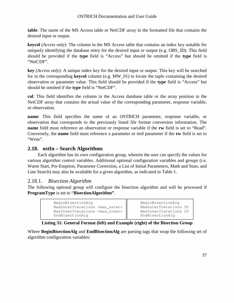
OSTRICH Documentation and User Guide
37
table: The name of the MS Access table or NetCDF array in the formatted file that contains the desired input or output.
keycol (Access only): The column in the MS Access table that contains an index key suitable for uniquely identifying the database entry for the desired input or output (e.g. OBS_ID). This field should be provided if the type field is “Access” but should be omitted if the type field is “NetCDF”.
key (Access only): A unique index key for the desired input or output. This key will be searched for in the corresponding keycol column (e.g. MW_01) to locate the tuple containing the desired observation or parameter value. This field should be provided if the type field is “Access” but should be omitted if the type field is “NetCDF”.
col: This field identifies the column in the Access database table or the array position in the NetCDF array that contains the actual value of the corresponding parameter, response variable, or observation.
name: This field specifies the name of an OSTRICH parameter, response variable, or observation that corresponds to the previously listed file format conversion information. The name field must reference an observation or response variable if the rw field is set to “Read”. Conversely, the name field must reference a parameter or tied parameter if the rw field is set to “Write”.
2.18. ostIn – Search Algorithms Each algorithm has its own configuration group, wherein the user can specify the values for
various algorithm control variables. Additional optional configuration variables and groups (i.e. Warm Start, Pre-Emption, Parameter Correction, a List of Initial Parameters, Math and Stats, and Line Search) may also be available for a given algorithm, as indicated in Table 1.
2.18.1. Bisection Algorithm The following optional group will configure the bisection algorithm and will be processed if ProgramType is set to “BisectionAlgorithm”.
Listing 31: General Format (left) and Example (right) of the Bisection Group
Where BeginBisectionAlg and EndBisectionAlg are parsing tags that wrap the following set of algorithm configuration variables:
BeginBisectionAlg MaxOuterIterations <max_outer> MaxInnerIterations <max_inner> EndBisectionAlg
BeginBisectionAlg MaxOuterIterations 50 MaxInnerIterations 20 EndBisectionAlg

OSTRICH Documentation and User Guide
38
MaxOuterIterations: The maximum number of outer iterations of the algorithm. One outer iteration corresponds to application of the bisection method to a randomly chosen initial parameter set. The default value is 50.
MaxInnerIterations: The maximum number of inner iterations of the algorithm. Each inner iteration reduces the searchable parameter range by 50%. Default value is 20.
2.18.2. Fletcher-Reeves The following optional group will configure the Fletcher-Reeves algorithm and will be processed if ProgramType is set to “Fletcher-Reeves”.
Listing 32: General Format (left) and Example (right) of the Fletcher-Reeves Group
Where BeginFletchReevesAlg and EndFletchReevesAlg are parsing tags that wrap the following set of algorithm configuration variables:
ConvergenceVal and MaxStalls: These variables control the convergence termination criterion for the algorithm. The algorithm will stop when the relative reduction in the objective function over max_stalls iterations is less than conv_val. The default value for conv_val is 1.00E-6 and the default value for max_stalls is 3.
MaxIterations: The maximum number of iterations of the algorithm. The default value is 20.
2.18.3. Gauss-Marquardt-Levenberg The following optional group will configure the Gauss-Marquardt-Levenberg algorithm and will be processed if ProgramType is set to “Levenberg-Marquardt”.
Listing 33: General Format of the Gauss-Marquardt-Levenberg Group
BeginFletchReevesAlg ConvergenceVal <conv_val> MaxStalls <max_stalls> MaxIterations <max_iter> EndFletchReevesAlg
BeginFletchReevesAlg ConvergenceVal 1.00E-6 MaxStalls 3 MaxIterations 20 EndFletchReevesAlg
BeginLevMar InitialLambda <init_lambda> LambdaScaleFactor <lambda_sf> MoveLimit <move_limit> AlgorithmConvergenceValue <conv_val> LambdaPhiRatio <phi_ratio> LambdaRelReduction <rel_reduce> MaxLambdas <max_lambda> MaxIterations <max_iters> EndLevMar

OSTRICH Documentation and User Guide
39
Where BeginLevMar and EndLevMar are parsing tags that wrap the following set of algorithm configuration variables:
InitialLambda: The initial Marquardt λ. The λ variable controls the algorithm’s transition from using a Steepest-Descent approach to using a Taylor Series approximation. The default is 10.00.
LambdaScaleFactor: The Marquardt λ scale factor – this is the factor by which λ is multiplied
or divided during λ adjustment. The default is 1.10.
MoveLimit: Parameter move limits – the maximum adjustment of a parameter (relative to the range of the parameter) that is allowed in a single iteration. The default is 0.10, or 10%.
AlgorithmConvergenceValue: The algorithm convergence value – regression will stop when the relative reduction in the objective function (i.e. phi, Φ) over two iterations is less than this value. The default value is 1.00E-4.
LambdaPhiRatio: This is the reduction criteria for deciding on optimal adjustments of the λ term. Adjustments for the given iteration are complete when the relative reduction in Φ is greater than this value. The default value is 0.30.
LambdaRelReduction: This is the reduction criteria for abandoning λ adjustment. Adjustments for the given iteration are halted when the relative reduction in Φ is less than this value. The default value is 0.01.
MaxLambdas: The maximum number of λ adjustments per iteration. The default value is 10.
MaxIterations: The maximum iterations in the overall method. The default value is 30.
2.18.4. Multi-Start GML with Trajectory Repulsion The following optional group will configure the Multi-Start Trajectory Repulsion Gauss-Marquardt-Levenberg algorithm and will be processed if ProgramType is set to “GML-MS”.

OSTRICH Documentation and User Guide
40
Listing 34: General Format of the Multi-Start GML Group
Where BeginLevMar and EndLevMar are parsing tags that wrap a set of algorithm configuration variables. Most of these variables are described above in Section 2.18.3 (Gauss-Marquardt-Levenberg). Additional variables related to multi-start capabilities are described below:
NumMultiStarts: The number of times the GML algorithm will be run using a different initial set of parameter values. The default value is 1 (i.e. no multi-starts).
2.18.5. Grid-based Exhaustive Search The following optional group will configure the Grid-based exhaustive search algorithm
and will be processed if ProgramType is set to “GridAlgorithm”.
Listing 35: General Format (left) and Example (right) of the Grid-based Search Group
Where BeginGridAlg and EndGridAlg are parsing tags that wrap the following set of algorithm configuration variables:
Dimensions: This variable describes a full-factorial sampling grid over which the exhaustive search will be applied. The sequence <d1 d2 … dn> should contain a space-separated list of “dimension” values for each parameter. The order of the values should correspond to the order in which parameters are listed in the Parameters group (see Section 2.7). The values represent the number of equally spaced samples that will be evaluated for each parameter. For example, consider if there were two parameters of interest: p1, with limits of -10 and +10, and p2, with limits of 0 and 100. A Dimensions entry of “Dimensions 5 3” would result in the evaluation of the following [p1, p2] parameter combinations:
p1 -10 -10 -10 -5 -5 -5 0 0 0 +5 +5 +5 +10 +10 +10 p2 0 50 100 0 50 100 0 50 100 0 50 100 0 50 100
BeginLevMar InitialLambda <init_lambda> LambdaScaleFactor <lambda_sf> MoveLimit <move_limit> AlgorithmConvergenceValue <conv_val> LambdaPhiRatio <phi_ratio> LambdaRelReduction <rel_reduce> MaxLambdas <max_lambda> MaxIterations <max_iters> NumMultiStarts <num_starts> EndLevMar
BeginGridAlg Dimensions <d1 d2 ... dn> EvalsPerIter <eval_per_itr> EndGridAlg
BeginGridAlg Dimensions 100 100 100 EvalsPerIter 1000 EndGridAlg
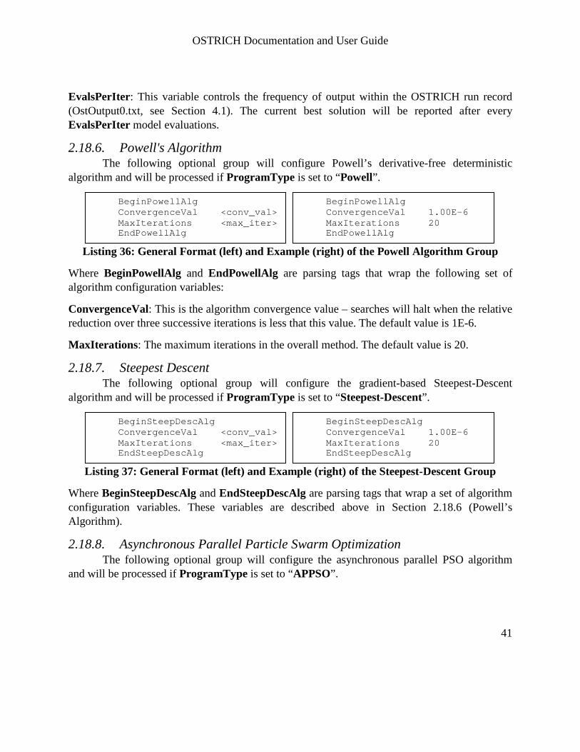
OSTRICH Documentation and User Guide
41
EvalsPerIter: This variable controls the frequency of output within the OSTRICH run record (OstOutput0.txt, see Section 4.1). The current best solution will be reported after every EvalsPerIter model evaluations.
2.18.6. Powell's Algorithm The following optional group will configure Powell’s derivative-free deterministic
algorithm and will be processed if ProgramType is set to “Powell”.
Listing 36: General Format (left) and Example (right) of the Powell Algorithm Group
Where BeginPowellAlg and EndPowellAlg are parsing tags that wrap the following set of algorithm configuration variables:
ConvergenceVal: This is the algorithm convergence value – searches will halt when the relative reduction over three successive iterations is less that this value. The default value is 1E-6.
MaxIterations: The maximum iterations in the overall method. The default value is 20.
2.18.7. Steepest Descent The following optional group will configure the gradient-based Steepest-Descent
algorithm and will be processed if ProgramType is set to “Steepest-Descent”.
Listing 37: General Format (left) and Example (right) of the Steepest-Descent Group
Where BeginSteepDescAlg and EndSteepDescAlg are parsing tags that wrap a set of algorithm configuration variables. These variables are described above in Section 2.18.6 (Powell’s Algorithm).
2.18.8. Asynchronous Parallel Particle Swarm Optimization The following optional group will configure the asynchronous parallel PSO algorithm
and will be processed if ProgramType is set to “APPSO”.
BeginPowellAlg ConvergenceVal <conv_val> MaxIterations <max_iter> EndPowellAlg
BeginPowellAlg ConvergenceVal 1.00E-6 MaxIterations 20 EndPowellAlg
BeginSteepDescAlg ConvergenceVal <conv_val> MaxIterations <max_iter> EndSteepDescAlg
BeginSteepDescAlg ConvergenceVal 1.00E-6 MaxIterations 20 EndSteepDescAlg

OSTRICH Documentation and User Guide
42
Listing 38: General Format (left) and Example (right) of the APPSO Algorithm Group
Where BeginAPPSO and EndAPPSO are parsing tags that wrap a set of algorithm configuration variables. These variables are described below:
SwarmSize: The size of the particle swarm. The default value is 20.
NumGenerations: The number of generations in the PSO. The default value is 50.
ConstrictionFactor: The value of χ in the PSO algorithm. Setting less than 1.00 will restrict the searchable design space after each iteration and accelerate convergence, but can lead to entrapment in local minima. The default value is 1.00.
CognitiveParam: The weight given to the local knowledge of each particle. High values (relative to the SocialParam) will cause particles to bias their search to the area surrounding each particles local best. The default value is 2.00.
SocialParam: The weight given to the global (social) knowledge of each particle. High values (relative to the CognitiveParam) will cause particles to bias their search to the area surrounding the global best. The default value is 2.00.
InertiaWeight: The initial weight given to the velocity used in each particle’s previous generation of movement. High values tend to cause particles to ’overshoot’ their destination, which is desirable in initial generations because it allows for more complete exploration of the design space. The default is 1.2.
InertiaReductionRate: Relative reduction rate for the inertia weight. As the optimization proceeds, the inertia weight is reduced by InertiaReductionRate × 100% of its current value. This reduces overshoot over successive generations such that late-generation searches are clustered around the global best solution. If this value is set to linear, the inertia weight will be linearly reduced from its initial value to a final value (i.e. at the last generation) of zero. The default value is 0.10.
BeginAPPSO SwarmSize <swarm> NumGenerations <ngen> ConstrictionFactor <cfact> CognitiveParam <cwght> SocialParam <swght> InertiaWeight <iwght> InertiaReductionRate <irate> EndAPPSO
BeginAPPSO SwarmSize 20 NumGenerations 50 ConstrictionFactor 1.00 CognitiveParam 2.00 SocialParam 2.00 InertiaWeight 1.20 InertiaReductionRate 0.10 EndAPPSO
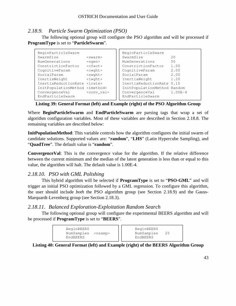
OSTRICH Documentation and User Guide
43
2.18.9. Particle Swarm Optimization (PSO) The following optional group will configure the PSO algorithm and will be processed if
ProgramType is set to “ParticleSwarm”.
Listing 39: General Format (left) and Example (right) of the PSO Algorithm Group
Where BeginParticleSwarm and EndParticleSwarm are parsing tags that wrap a set of algorithm configuration variables. Most of these variables are described in Section 2.18.8. The remaining variables are described below:
InitPopulationMethod: This variable controls how the algorithm configures the initial swarm of candidate solutions. Supported values are: “random”, “LHS” (Latin Hypercube Sampling), and “QuadTree”. The default value is “random”.
ConvergenceVal: This is the convergence value for the algorithm. If the relative difference between the current minimum and the median of the latest generation is less than or equal to this value, the algorithm will halt. The default value is 1.00E-4.
2.18.10. PSO with GML Polishing This hybrid algorithm will be selected if ProgramType is set to “PSO-GML” and will
trigger an initial PSO optimization followed by a GML regression. To configure this algorithm, the user should include both the PSO algorithm group (see Section 2.18.9) and the Gauss-Marquardt-Levenberg group (see Section 2.18.3).
2.18.11. Balanced Exploration-Exploitation Random Search The following optional group will configure the experimental BEERS algorithm and will
be processed if ProgramType is set to “BEERS”.
Listing 40: General Format (left) and Example (right) of the BEERS Algorithm Group
BeginParticleSwarm SwarmSize <swarm> NumGenerations <ngen> ConstrictionFactor <cfact> CognitiveParam <cwght> SocialParam <swght> InertiaWeight <iwght> InertiaReductionRate <irate> InitPopulationMethod <imethod> ConvergenceVal <conv_val> EndParticleSwarm
BeginParticleSwarm SwarmSize 20 NumGenerations 50 ConstrictionFactor 1.00 CognitiveParam 2.00 SocialParam 2.00 InertiaWeight 1.20 InertiaReductionRate 0.10 InitPopulationMethod Random ConvergenceVal 1.00E-4 EndParticleSwarm
BeginBEERS NumSamples <nsamp> EndBEERS
BeginBEERS NumSamples 25 EndBEERS
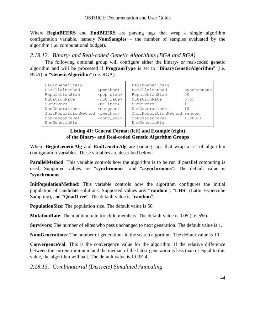
OSTRICH Documentation and User Guide
44
Where BeginBEERS and EndBEERS are parsing tags that wrap a single algorithm configuration variable, namely NumSamples – the number of samples evaluated by the algorithm (i.e. computational budget).
2.18.12. Binary- and Real-coded Genetic Algorithms (BGA and RGA) The following optional group will configure either the binary- or real-coded genetic
algorithm and will be processed if ProgramType is set to “BinaryGeneticAlgorithm” (i.e. BGA) or “GeneticAlgorithm” (i.e. RGA).
Listing 41: General Format (left) and Example (right)
of the Binary- and Real-coded Genetic Algorithm Groups
Where BeginGeneticAlg and EndGeneticAlg are parsing tags that wrap a set of algorithm configuration variables. These variables are described below:
ParallelMethod: This variable controls how the algorithm is to be run if parallel computing is used. Supported values are “synchronous” and “asynchronous”. The default value is “synchronous”.
InitPopulationMethod: This variable controls how the algorithm configures the initial population of candidate solutions. Supported values are: “random”, “LHS” (Latin Hypercube Sampling), and “QuadTree”. The default value is “random”.
PopulationSize: The population size. The default value is 50.
MutationRate: The mutation rate for child members. The default value is 0.05 (i.e. 5%).
Survivors: The number of elites who pass unchanged to next generation. The default value is 1.
NumGenerations: The number of generations in the search algorithm. The default value is 10.
ConvergenceVal: This is the convergence value for the algorithm. If the relative difference between the current minimum and the median of the latest generation is less than or equal to this value, the algorithm will halt. The default value is 1.00E-4.
2.18.13. Combinatorial (Discrete) Simulated Annealing
BeginGeneticAlg ParallelMethod <pmethod> PopulationSize <pop_size> MutationRate <mut_rate> Survivors <nelites> NumGenerations <numgens> InitPopulationMethod <imethod> ConvergenceVal <conv_val> EndGeneticAlg
BeginGeneticAlg ParallelMethod synchronous PopulationSize 50 MutationRate 0.05 Survivors 1 NumGenerations 10 InitPopulationMethod random ConvergenceVal 1.00E-4 EndGeneticAlg
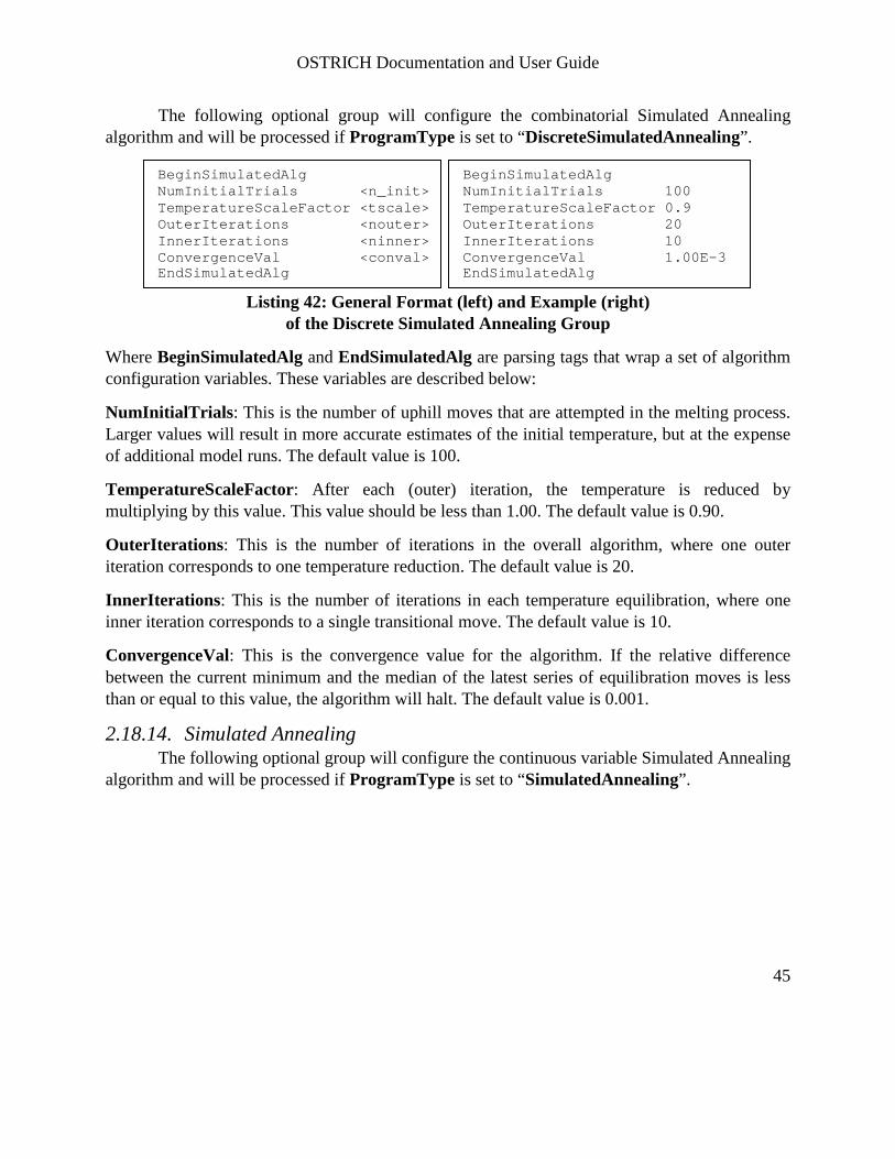
OSTRICH Documentation and User Guide
45
The following optional group will configure the combinatorial Simulated Annealing algorithm and will be processed if ProgramType is set to “DiscreteSimulatedAnnealing”.
Listing 42: General Format (left) and Example (right)
of the Discrete Simulated Annealing Group
Where BeginSimulatedAlg and EndSimulatedAlg are parsing tags that wrap a set of algorithm configuration variables. These variables are described below:
NumInitialTrials: This is the number of uphill moves that are attempted in the melting process. Larger values will result in more accurate estimates of the initial temperature, but at the expense of additional model runs. The default value is 100.
TemperatureScaleFactor: After each (outer) iteration, the temperature is reduced by multiplying by this value. This value should be less than 1.00. The default value is 0.90.
OuterIterations: This is the number of iterations in the overall algorithm, where one outer iteration corresponds to one temperature reduction. The default value is 20.
InnerIterations: This is the number of iterations in each temperature equilibration, where one inner iteration corresponds to a single transitional move. The default value is 10.
ConvergenceVal: This is the convergence value for the algorithm. If the relative difference between the current minimum and the median of the latest series of equilibration moves is less than or equal to this value, the algorithm will halt. The default value is 0.001.
2.18.14. Simulated Annealing The following optional group will configure the continuous variable Simulated Annealing
algorithm and will be processed if ProgramType is set to “SimulatedAnnealing”.
BeginSimulatedAlg NumInitialTrials <n_init> TemperatureScaleFactor <tscale> OuterIterations <nouter> InnerIterations <ninner> ConvergenceVal <conval> EndSimulatedAlg
BeginSimulatedAlg NumInitialTrials 100 TemperatureScaleFactor 0.9 OuterIterations 20 InnerIterations 10 ConvergenceVal 1.00E-3 EndSimulatedAlg

OSTRICH Documentation and User Guide
46
Listing 43: General Format (left) and Example (right)
of the Continuous Variable Simulated Annealing Group
Where BeginSimulatedAlg and EndSimulatedAlg are parsing tags that wrap a set of algorithm configuration variables. Most of these variables are described in Section 2.18.13. The remaining variables are described below:
FinalTemperature: This variable can be used to set a specific value for the final temperature in the SA algorithm. The temperature scale factor will be adjusted to achieve the desired temperature. Alternatively, OSTRICH supports two options for dynamically pre-computing the final temperature. These dynamic options are based on the methods of Vanderbilt and Louie (1984) and Ben-Ameur (2004), respectively. Set the FinalTemperature to “computed-vanderbilt” to select the Vanderbilt-Louie approach. Set the FinalTemperature to “compute-ben-ameur” to select the Ben-Ameur approach. If a final temperature option or value is not specified, the final temperature will be determined from the initial temperature, temperature scale factor, and number of outer iterations.
TransitionMethod: This variable selects the method used to compute randomized parameter perturbations during the transition phase of the SA algorithm. Set this variable to “Uniform” to sample from a uniform distribution, or use a value of “Gauss” to select a Gaussian (i.e. normal) distribution. The default value is “Gauss”.
2.18.15. Vanderbilt-Louie Simulated Annealing The following optional group will configure the continuous variable Vanderbilt-Louie
variant of the Simulated Annealing algorithm and will be processed if ProgramType is set to “VanderbiltSimulatedAnnealing”.
BeginSimulatedAlg NumInitialTrials <n_init> TemperatureScaleFactor <tscale> OuterIterations <nouter> InnerIterations <ninner> ConvergenceVal <conval> FinalTemperature <tfinal> TransitionMethod <tmethd> EndSimulatedAlg
BeginSimulatedAlg NumInitialTrials 100 TemperatureScaleFactor 0.9 OuterIterations 20 InnerIterations 10 ConvergenceVal 1.00E-3 FinalTemperature 10.0 TransitionMethod Gauss EndSimulatedAlg

OSTRICH Documentation and User Guide
47
Listing 44: General Format (left) and Example (right) of the Vanderbilt-Louie Simulated Annealing Group
Where BeginSimulatedAlg and EndSimulatedAlg are parsing tags that wrap a set of algorithm configuration variables. Most of these variables are described in Section 2.18.13. The remaining variables are described below:
FinalTemperature: This variable can be used to set a specific value for the final temperature in the SA algorithm. The temperature scale factor will be adjusted to achieve the desired temperature. If a final temperature option or value is not specified, the final temperature will be determined from the initial melting phase using a procedure described by Vanderbilt and Louie (1984).
TransitionMethod: This variable selects the method used to compute randomized parameter perturbations during the transition phase of the SA algorithm. Set this variable to “Vanderbilt” to sample according to the procedure outlined by Vanderbilt and Louie (1984). Use a value of “Gauss” to select a Gaussian (i.e. normal) distribution. The default value is “Gauss”.
2.18.16. Discrete DDS The following optional group will configure the discrete DDS algorithm and will be
processed if ProgramType is set to “DiscreteDDS”.
Listing 45: General Format (left) and Example (right) of the Discrete DDS Group
Where BeginDiscreteDDSAlg and EndDiscreteDDSAlg are parsing tags that wrap a set of algorithm configuration variables. These variables are described below:
PerturbationValue: This parameter defines the standard deviation of the decision variable perturbations as follows: PerturbationValue = StdDev / DV_Range. The allowable range is 0 to
BeginSimulatedAlg NumInitialTrials <n_init> TemperatureScaleFactor <tscale> OuterIterations <nouter> InnerIterations <ninner> ConvergenceVal <conval> FinalTemperature <tfinal> TransitionMethod <tmethd> EndSimulatedAlg
BeginSimulatedAlg NumInitialTrials 100 TemperatureScaleFactor 0.9 OuterIterations 20 InnerIterations 10 ConvergenceVal 1.00E-3 FinalTemperature 10.0 TransitionMethod Gauss EndSimulatedAlg
BeginDiscreteDDSAlg PerturbationValue <r_val> MaxIterations <budget> UseInitialParamValues UseRandomParamValues EndDiscreteDDSAlg
BeginDiscreteDDSAlg PerturbationValue 0.2 MaxIterations 100 UseRandomParamValues EndDiscreteDDSAlg
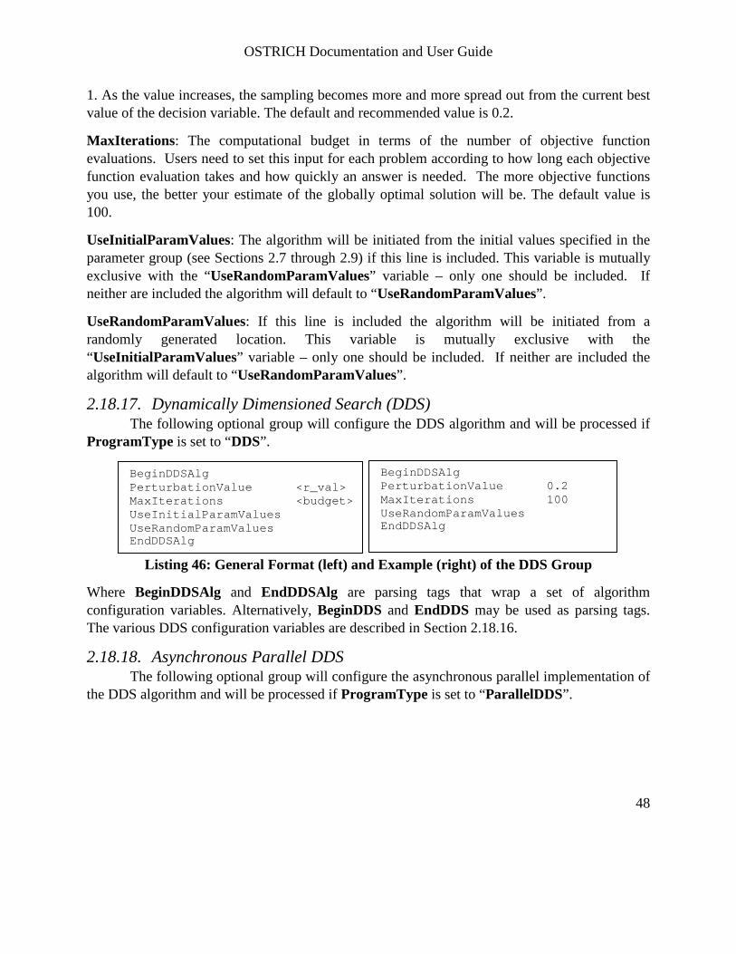
OSTRICH Documentation and User Guide
48
1. As the value increases, the sampling becomes more and more spread out from the current best value of the decision variable. The default and recommended value is 0.2.
MaxIterations: The computational budget in terms of the number of objective function evaluations. Users need to set this input for each problem according to how long each objective function evaluation takes and how quickly an answer is needed. The more objective functions you use, the better your estimate of the globally optimal solution will be. The default value is 100.
UseInitialParamValues: The algorithm will be initiated from the initial values specified in the parameter group (see Sections 2.7 through 2.9) if this line is included. This variable is mutually exclusive with the “UseRandomParamValues” variable – only one should be included. If neither are included the algorithm will default to “UseRandomParamValues”.
UseRandomParamValues: If this line is included the algorithm will be initiated from a randomly generated location. This variable is mutually exclusive with the “UseInitialParamValues” variable – only one should be included. If neither are included the algorithm will default to “UseRandomParamValues”.
2.18.17. Dynamically Dimensioned Search (DDS) The following optional group will configure the DDS algorithm and will be processed if
ProgramType is set to “DDS”.
Listing 46: General Format (left) and Example (right) of the DDS Group
Where BeginDDSAlg and EndDDSAlg are parsing tags that wrap a set of algorithm configuration variables. Alternatively, BeginDDS and EndDDS may be used as parsing tags. The various DDS configuration variables are described in Section 2.18.16.
2.18.18. Asynchronous Parallel DDS The following optional group will configure the asynchronous parallel implementation of
the DDS algorithm and will be processed if ProgramType is set to “ParallelDDS”.
BeginDDSAlg PerturbationValue <r_val> MaxIterations <budget> UseInitialParamValues UseRandomParamValues EndDDSAlg
BeginDDSAlg PerturbationValue 0.2 MaxIterations 100 UseRandomParamValues EndDDSAlg

OSTRICH Documentation and User Guide
49
Listing 47: General Format (left) and Example (right) of the parallel DDS Group
Where BeginParallelDDSAlg and EndParallelDDSAlg are parsing tags that wrap a set of algorithm configuration variables. Other acceptable parsing tags are:
• BeginParallelDDS and EndParallelDDS • BeginParaDDSAlg and EndParaDDSAlg • BeginParaDDS and EndParaDDS • BeginDDSAlg and EndDDSAlg • BeginDDS and EndDDS
Several of the parallel DDS configuration variables (i.e. PerturbationValue, MaxIterations, UseInitialParamValues, and UseRandomParamValues) are described in Section 2.18.16. The remaining variables are described below:
UseOpt: Users wanting to apply the original DDS algorithm can ignore specifying this option. This option is used by OSTRICH and DDS developers to compare the DDS algorithm implemented in different programming languages. It is an experimental developer option that controls the calculation of parameter adjustments within the parallel DDS algorithm. Three values are acceptable: “no-rand-num”, “try-int-solution”, and “standard”. The default and recommended value is “standard”. The “Alpha” and “Beta” values will be used by the algorithm if “no-rand-num” is selected. Otherwise, these variables are ignored (i.e. if either “try-int-solution” or “standard” are selected).
AlphaValue and BetaValue: These parameters control the parallel DDS perturbation scheme if the UseOpt variable is set to “no-rand-num”. Otherwise, these variables are ignored. Both variables have a default value of 0.5.
EnableDebugging: The parallel DDS algorithm will report additional development-level debugging information if this variable is included. The default behavior of the algorithm is to not report debugging information.
BeginParallelDDSAlg PerturbationValue <r_val> MaxIterations <budget> UseInitialParamValues UseRandomParamValues UseOpt <option> AlphaValue <alpha> BetaValue <beta> EnableDebugging EndParallelDDSAlg
BeginParallelDDSAlg PerturbationValue 0.2 MaxIterations 100 UseRandomParamValues UseOpt standard EndParallelDDSAlg

OSTRICH Documentation and User Guide
50
2.18.19. Shuffled Complex Evolution (SCE) The following optional group will configure the shuffled complex evolution (SCE)
algorithm and will be processed if ProgramType is set to “ShuffledComplexEvolution”.
Listing 48: General Format (left) and Example (right) of the SCE Group
Where BeginSCEUA and EndSCEUA are parsing tags that wrap a set of algorithm configuration variables. These variables are described below and descriptions are based on comments within the FORTRAN implementation provided by Duan et al. (1993). The corresponding variable names used in the FORTRAN implementation are provided in brackets (‘<’ and ‘>’) in the general format of Listing 48.
Budget (MAXN): Maximum number of trials allowed before optimization is terminated. The purpose of MAXN is to stop an optimization search before too much computer time is expended. MAXN should be set large enough so that optimization is generally completed before MAXN trials are performed. Recommended value is 10,000 (increase or decrease as necessary). LoopStagnationCriteria (KSTOP): Number of shuffling loops in which the optimization criterion must improve by the specified percentage or else optimization will be restarted. PctChangeCriteria (PCENTO): Percentage by which the optimization criterion value must change in the specified number of shuffling loops or else optimization is restarted. Use decimal equivalent: Percentage/100. Recommended value: 0.01. PopConvCriteria (PEPS): The optimization will be restarted if the shuffling and/or evolution process results in a population that is entirely within PEPS×100 percent of the feasible space. The default value is 0.001. NumComplexes (NGS): Number of complexes used for optimization search. Minimum value is 1. Recommended value is between 2 and 20 depending on the number of parameters to be optimized and on the degree of difficulty of the problem. If not specified OSTRICH will use the following calculation: NGS = sqrt(np) , where np is the number of parameters.
BeginSCEUA Budget <MAXN> LoopStagnationCriteria <KSTOP> PctChangeCriteria <PCENTO> PopConvCriteria <PEPS> NumComplexes <NGS> NumPointsPerComplex <NPG> NumPointsPerSubComplex <NPS> NumEvolutionSteps <NSPL> MinNumberOfCOmplexes <MINGS> UseInitialPoint <INIFLG> EndSCEUA
BeginSCEUA Budget 10000 LoopStagnationCriteria 5 PctChangeCriteria 0.01 PopConvCriteria 0.001 NumComplexes 3 NumPointsPerComplex 19 NumPointsPerSubComplex 10 NumEvolutionSteps 19 MinNumberOfCOmplexes 3 UseInitialPoint no EndSCEUA
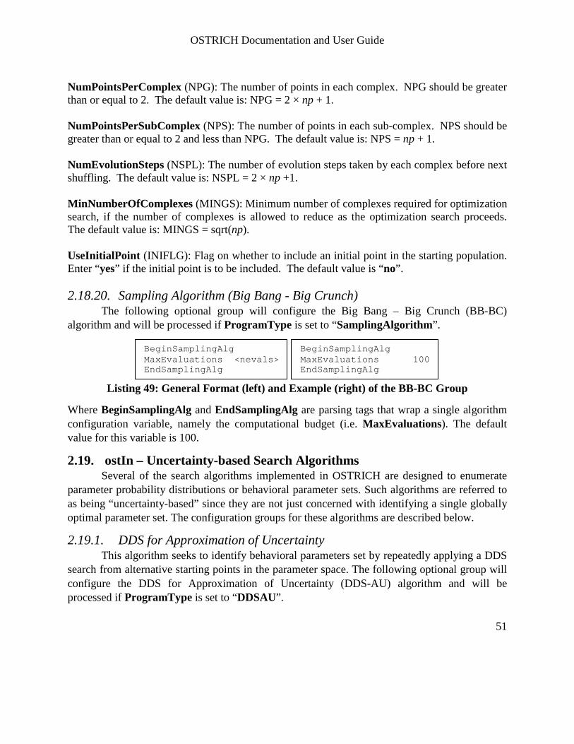
OSTRICH Documentation and User Guide
51
NumPointsPerComplex (NPG): The number of points in each complex. NPG should be greater than or equal to 2. The default value is: NPG = 2 × np + 1. NumPointsPerSubComplex (NPS): The number of points in each sub-complex. NPS should be greater than or equal to 2 and less than NPG. The default value is: NPS = np + 1. NumEvolutionSteps (NSPL): The number of evolution steps taken by each complex before next shuffling. The default value is: NSPL = 2 × np +1. MinNumberOfComplexes (MINGS): Minimum number of complexes required for optimization search, if the number of complexes is allowed to reduce as the optimization search proceeds. The default value is: MINGS = sqrt(np). UseInitialPoint (INIFLG): Flag on whether to include an initial point in the starting population. Enter “yes” if the initial point is to be included. The default value is “no”. 2.18.20. Sampling Algorithm (Big Bang - Big Crunch)
The following optional group will configure the Big Bang – Big Crunch (BB-BC) algorithm and will be processed if ProgramType is set to “SamplingAlgorithm”.
Listing 49: General Format (left) and Example (right) of the BB-BC Group
Where BeginSamplingAlg and EndSamplingAlg are parsing tags that wrap a single algorithm configuration variable, namely the computational budget (i.e. MaxEvaluations). The default value for this variable is 100.
2.19. ostIn – Uncertainty-based Search Algorithms Several of the search algorithms implemented in OSTRICH are designed to enumerate
parameter probability distributions or behavioral parameter sets. Such algorithms are referred to as being “uncertainty-based” since they are not just concerned with identifying a single globally optimal parameter set. The configuration groups for these algorithms are described below.
2.19.1. DDS for Approximation of Uncertainty This algorithm seeks to identify behavioral parameters set by repeatedly applying a DDS
search from alternative starting points in the parameter space. The following optional group will configure the DDS for Approximation of Uncertainty (DDS-AU) algorithm and will be processed if ProgramType is set to “DDSAU”.
BeginSamplingAlg MaxEvaluations <nevals> EndSamplingAlg
BeginSamplingAlg MaxEvaluations 100 EndSamplingAlg

OSTRICH Documentation and User Guide
52
Listing 50: General Format (left) and Example (right) of the DDS-AU Group
Where Begin_DDSAU_Alg and End_DDSAU_Alg are parsing tags that wrap a set of algorithm configuration variables. These variables are described below:
PerturbationValue: This parameter defines the standard deviation of the decision variable perturbations as follows: PerturbationValue = StdDev / DV_Range. The allowable range is 0 to 1. As the value increases, the sampling becomes more and more spread out from the current best value of the decision variable. The default and recommended value is 0.2.
NumSearches: The number of independent DDS searches to perform as part of the overall DDS-AU uncertainty approximation algorithm. The default value is 25. Each search will be run using either the DDS algorithm (Section 2.18.17) or the asynchronous parallel DDS algorithm (Section 2.18.18), depending on the value assigned to the ParallelSearches variable. Results for each search will be stored in output files named OstModel[N]_DDS[M].txt and OstOutput[N]_DDS[M].txt, where [N] is the processor number and [M] is the DDS search number. A DDS-AU summary file named OstOutputDDSAU.txt will be created when all DDS searches are complete. This file will contain results of the various optimization trials as well as a summary of the behavioral parameter sets that were discovered.
MinItersPerSearch and MaxItersPerSearch: The minimum and maximum computational budget for each independent DDS search. If the same budget is desired for each search, assign the desired value to both MinItersPerSearch and MaxItersPerSearch. If different values are assigned to these variables, the DDS-AU algorithm will randomly generate a different budget for each search. The randomly generated budget will fall within the range specified by MinItersPerSearch and MaxItersPerSearch. The default value for MinItersPerSearch is 30. The default value for MaxItersPerSearch is 70.
ParallelSearches: Each independent search will be run using the asynchronous parallel DDS algorithm if this variable is set to “yes”. Otherwise, each independent search will be run using a serial implementation of the DDS algorithm. The default value is “no”.
Begin_DDSAU_Alg PerturbationValue <r_val> NumSearches <nsols> MinItersPerSearch <imin> MaxItersPerSearch <imax> ParallelSearches yes|no Threshold <fmax> Randomize yes|no ReviseAU yes|no End_DDSAU_Alg
Begin_DDSAU_Alg PerturbationValue 0.2 NumSearches 25 MinItersPerSearch 30 MaxItersPerSearch 70 ParallelSearches no Threshold 1000 Randomize no ReviseAU yes End_DDSAU_Alg
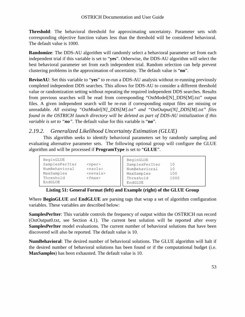
OSTRICH Documentation and User Guide
53
Threshold: The behavioral threshold for approximating uncertainty. Parameter sets with corresponding objective function values less than the threshold will be considered behavioral. The default value is 1000.
Randomize: The DDS-AU algorithm will randomly select a behavioral parameter set from each independent trial if this variable is set to “yes”. Otherwise, the DDS-AU algorithm will select the best behavioral parameter set from each independent trial. Random selection can help prevent clustering problems in the approximation of uncertainty. The default value is “no”.
ReviseAU: Set this variable to “yes” to re-run a DDS-AU analysis without re-running previously completed independent DDS searches. This allows for DDS-AU to consider a different threshold value or randomization setting without repeating the required independent DDS searches. Results from previous searches will be read from corresponding “OstModel[N]_DDS[M].txt” output files. A given independent search will be re-run if corresponding output files are missing or unreadable. All existing “OstModel[N]_DDS[M].txt” and “OstOutput[N]_DDS[M].txt” files found in the OSTRICH launch directory will be deleted as part of DDS-AU initialization if this variable is set to “no”. The default value for this variable is “no”.
2.19.2. Generalized Likelihood Uncertainty Estimation (GLUE) This algorithm seeks to identify behavioral parameters set by randomly sampling and
evaluating alternative parameter sets. The following optional group will configure the GLUE algorithm and will be processed if ProgramType is set to “GLUE”.
Listing 51: General Format (left) and Example (right) of the GLUE Group
Where BeginGLUE and EndGLUE are parsing tags that wrap a set of algorithm configuration variables. These variables are described below:
SamplesPerIter: This variable controls the frequency of output within the OSTRICH run record (OstOutput0.txt, see Section 4.1). The current best solution will be reported after every SamplesPerIter model evaluations. The current number of behavioral solutions that have been discovered will also be reported. The default value is 10.
NumBehavioral: The desired number of behavioral solutions. The GLUE algorithm will halt if the desired number of behavioral solutions has been found or if the computational budget (i.e. MaxSamples) has been exhausted. The default value is 10.
BeginGLUE SamplesPerIter <nper> NumBehavioral <nsols> MaxSamples <nevals> Threshold <fmax> EndGLUE
BeginGLUE SamplesPerIter 10 NumBehavioral 10 MaxSamples 100 Threshold 1000 EndGLUE

OSTRICH Documentation and User Guide
54
MaxSamples: The maximum number of model evaluations allowed before the GLUE search is terminated. The default value is 100. However, studies have shown that GLUE can require 100,000 or more evaluations to discover a sufficiently representative number of behavioral samples.
Threshold: The threshold for separating behavioral and non-behavioral parameter sets. Parameter sets with corresponding objective function values less than the threshold will be considered behavioral. The default value is 1000.
2.19.3. Metropolis-Hastings Markov Chain Monte Carlo (MCMC) This algorithm seeks to identify parameter probability distributions using a Bayesian
Markov Chain Monte Carlo (MCMC) sampler. It is based on the Metropolis-Hastings algorithm described by Kuczera and Parent (1998). The sampler seeks to evolve an initial set of truncated uniform distributions into the correct posterior probability distribution for each parameter. The following optional group will configure the Metropolis-Hastings MCMC algorithm and will be processed if ProgramType is set to “MetropolisSampler”.
Listing 52: General Format (left) and Example (right) of the MCMC Group
Where BeginMetropolisSampler and EndMetropolisSampler are parsing tags that wrap a set of algorithm configuration variables. These variables are described below:
SamplesPerIter: This variable controls the frequency of output within the OSTRICH run record (OstOutput0.txt, see Section 4.1). The current best solution will be reported after every SamplesPerIter model evaluations. The current number of accepted solutions will also be reported. Samples that are accepted after the burn-in period is complete are understood to come from a posterior distribution. The default value is 10.
NumDesired: The desired number of post burn-in samples (i.e. the number of samples that are desired from the posterior parameter distributions). The default value is 10.
BurnInSamples: The number of accepted samples that should be discarded before assuming accepted samples are representative of a posterior distribution. The default value is 0 (i.e. no burn-in).
BeginMetropolisSampler SamplesPerIter <nper> NumDesired <nsols> BurnInSamples <nburn> MaxSamples <nmax> LikelihoodType <ltype> ShapingFactor <shape> TelescopeRate <trate> EndMetropolisSampler
BeginMetropolisSampler SamplesPerIter 10 NumDesired 10 BurnInSamples 0 MaxSamples 100 LikelihoodType Stedinger ShapingFactor 0.5 TelescopeRate 0 EndMetropolisSampler

OSTRICH Documentation and User Guide
55
MaxSamples: The maximum number of model evaluations that will be performed as part of the MCMC search. The default value is 100.
LikelihoodType: Use this variable to select alternative formulations for computing the likelihood ratio. Two options are available, namely “Beven” and “Stedinger”. The Beven likelihood type is a pseudo-likelihood described by Beven and Binley (1992). The “Stedinger” likelihood type is a formal likelihood function described by Stedinger et al. (2008). If “Beven” is selected, the ShapingFactor (see below) will also be processed. The default setting is Stedinger.
ShapingFactor: This variable is a correction exponent for the Beven pseudo-likelihood function. As described by Stedinger et al. (2008), adjusting the ShapingFactor can help remove bias when using the “Beven” approach to computing likelihood ratios. The default value is 0.5, corresponding to a root-mean-squared-error type of likelihood function.
TelescopeRate: This variable is the fraction by which to constrict parameter bounds after each iteration. It can increase the acceptance rate by focusing the sampler on high-probability regions of the parameter space. The default value is 0 (i.e. no telescoping).
2.19.4. Rejection Sampling This algorithm seeks to identify parameter probability distributions using a rejection
sampling procedure. It is based on the procedure described by Chen (2005). The algorithm samples from a set of truncated uniform distributions in search of parameter sets that are representative of the “true” posterior probability distribution. It represents a middle ground between informal GLUE-like procedures, including DDS-AU, and formal MCMC procedures. The following optional group will configure the Rejection Sampling algorithm and will be processed if ProgramType is set to “RejectionSampler”.
Listing 53: General Format (left) and Example (right) of the Rejection Sampler Group
Where BeginRejectionSampler and EndRejectionSampler are parsing tags that wrap a set of algorithm configuration variables. Except for MinWSSE, these variables are described in Section 2.19.3. The MinWSSE variable is the calibrated (i.e. minimized) weighted sum of squared error objective function for the model. The default value is 1.00E308 (i.e. infinity).
BeginRejectionSampler SamplesPerIter <nper> NumDesired <nsols> BurnInSamples <nburn> MaxSamples <nmax> LikelihoodType <ltype> ShapingFactor <shape> TelescopeRate <trate> MinWSSE <wsse> EndRejectionSampler
BeginRejectionSampler SamplesPerIter 10 NumDesired 10 BurnInSamples 0 MaxSamples 100 LikelihoodType Stedinger ShapingFactor 0.5 TelescopeRate 0 MinWSSE 1.00E308 EndRejectionSampler

OSTRICH Documentation and User Guide
56
Users should replace this value with the results of a calibration algorithm, such as those described in Sections 2.18.1 to 2.18.20.
2.20. ostIn – Multi-Objective Search Algorithms The algorithms described below seek to identify non-dominated solutions representing
the tradeoff curve (i.e. pareto front) among conflicting objectives. These objectives can reflect a multi-criteria calibration exercise or a multi-objective optimization problem.
2.20.1. Pareto Archived DDS (PADDS) The following optional group will configure the multi-objective Pareto Archived DDS
algorithm and will be processed if ProgramType is set to “PADDS”.
Listing 54: General Format (left) and Example (right) of the PADDS Group
Where BeginPADDSAlg and EndPADDSAlg are parsing tags that wrap a set of algorithm configuration variables. Alternatively, BeginPADDS and EndPADDS may be used as the parsing tags. PADDS configuration variables are described below:
PerturbationValue: This parameter defines the standard deviation of the decision variable perturbations as follows: PerturbationValue = StdDev / DV_Range. The allowable range is 0 to 1. As the value increases, the sampling becomes more and more spread out from the current best value of the decision variable. The default and recommended value is 0.2.
MaxIterations: The computational budget in terms of the number of objective function evaluations. Users need to set this input for each problem according to how long each objective function evaluation takes and how quickly an answer is needed. The more objective functions you use, the better your estimate of the globally optimal solution will be. The default value is 50.
SelectionMetric: This metric for scoring non-dominated solutions when seeding DDS trials within the overall PADDS algorithm. Values currently supported are listed below:
• Random • CrowdingDistance • EstimatedHyperVolumeContribution • ExactHyperVolumeContribution
The default selection metric value is “ExactHyperVolumeContribution”. For a discussion on choosing the appropriate selection metric see Asadzadeh and Tolson (2013).
BeginPADDSAlg PerturbationValue <r_val> MaxIterations <budget> SelectionMetric <metric> EndPADDSAlg
BeginPADDSAlg PerturbationValue 0.2 MaxIterations 50 SelectionMetric Random EndPADDSAlg

OSTRICH Documentation and User Guide
57
2.20.2. Asynchronous Parallel PADDS The following optional group will configure a parallelized version of the PADDS
algorithm and will be processed if ProgramType is set to “ParaPADDS”.
Listing 55: General Format (left) and Example (right) of the parallel PADDS Group
Where BeginParallelPADDSAlg and EndParallelPADDSAlg are parsing tags that wrap a set of algorithm configuration variables. These variables are described in Section 2.20.1. Other acceptable parsing tags are:
• BeginParallelPADDS and EndParallelPADDS • BeginParaPADDSAlg and EndParaPADDSAlg • BeginParaPADDS and EndParaPADDS • BeginPADDSAlg and EndPADDSAlg • BeginPADDS and EndPADDS
2.20.3. Simple Multi-Objective Optimization Test Heuristic (SMOOTH) The following optional group will configure an experimental multi-objective algorithm
known as SMOOTH and will be processed if ProgramType is set to “SMOOTH”.
Listing 56: General Format (left) and Example (right) of the SMOOTH Group
SamplesPerIter: The number of model evaluations per iteration of the algorithm.
NumIterations: The number of iterations in the algorithm.
2.21. ostIn – Math and Stats This group describes the finite difference method employed by algorithms in Table 1 with
shaded entries in the “Math and Stats?” column. If calibration is being performed, additional variables in this group are used to request various statistical and diagnostic output. The general format of the MathAndStats group is given in Listing 58 and Listing 58 is a concrete example.
BeginParallelPADDSAlg PerturbationValue <r_val> MaxIterations <budget> SelectionMetric <metric> EndParallelPADDSAlg
BeginParallelPADDSAlg PerturbationValue 0.2 MaxIterations 50 SelectionMetric Random EndParallelPADDSAlg
BeginSMOOTH SamplesPerIter <nsamp> NumIterations <niter> EndSMOOTH
BeginSMOOTH SamplesPerIter 20 NumIterations 50 EndSMOOTH

OSTRICH Documentation and User Guide
58
Listing 57: General Format of the Math and Stats Group
As shown in Listing 57, a “Predictions” sub-group can be used to instruct OSTRICH to compute confidence limits on predicted quantities of a calibrated model. The format of the Predictions sub-group is identical to the Response Variables group (see Section 2.15).
Listing 58: Example of the Math and Stats Group
Variables in the Math and Stats group are described below:
DiffType: This variable selects the type of finite-difference approach to use for approximating derivatives (i.e. ∂Y/∂p, where Y is some model output and p is a parameter). Options are “forward” (forward differences), “outside” (outside central differences), “parabolic” (parabolic central differences), and “best-fit” (linear central differences). Central differences require twice as much computation as forward differences but can be more accurate. The default value is “forward”.
BeginMathAndStats DiffType <dtype> DiffIncType <ditype> DiffRelIncrement <drinc> DIffIncrement <dinc> DiffMinIncrement <dmin> CI_Pct <cipct> <Stat1> . . . <StatN> BeginPredictions --- see section 2.15 EndPredictions EndMathAndStats
BeginMathAndStats DiffType forward DiffIncType value-relative DIffIncrement 0.01 DiffMinIncrement 1.00E-6 CI_Pct 0.95 AllStats ExcludeInsensitiveParameters ExcludeInsensitiveObservations BeginPredictions
#name filename key line col token augmented? MinDef CanBeam.out ; Umin 2 2 '=' no
MaxDef CanBeam.out ; Umax 3 2 '=' no EndPredictions EndMathAndStats
OSTRICH Documentation and User Guide
59
DiffIncType: The type of increment used in the selected finite-difference approach. Supported values for this variable are described below, and the default is “range-relative”:
range-relative: Increments will be computed by multiplying the range of a given parameter by the value of the“DiffIncrement” or “DiffRelIncrement” variable.
value-relative: Increments will be computed by multiplying the current value of a given parameter by the value of the “DiffIncrement” variable.
absolute: Increments will be directly specified by the value of the “DiffIncrement” variable.
optimal: Finite-difference increments will be computed according to the iterative procedure outlined by Yager (2004).
DiffRelIncrement: When this variable is assigned the program will use a range-relative finite-difference increment, irrespective of the value of DiffIncType. The value of this variable can be a single value that will be applied to each parameter, or a space-separated list of values corresponding to each parameter listed in the parameters group (see Section 2.7). The default value is 0.001 for all parameters.
DiffIncrement: The value used in computing a finite-difference for each parameter. The value of this variable can be a single value that will be applied to each parameter, or a space-separated list of values corresponding to each parameter listed in the parameters group (see Section 2.7). The default value is 0.001 for all parameters.
DiffMinIncrement: The minimum increment that will be used irrespective of the compute valued. The default value is 1.00E-20.
CI_Pct: The desired confidence level for computing linear confidence intervals on parameters and predictions. The default value is 95.
Stat1 .. StatN: These entries serve as flags to select various statistical output. Options are described below. The default flags are “NoStats”, “ExcludeInsensitiveParameters”, and “ExcludeInsensitiveObservations”:
Default: Selects a default list of parameter statistics, including correlation, standard error, and linear confidence intervals.
AllStats: Enables all available statistical output.
NoStats: Disables all statistical output.
BestBoxCox: Instructs OSTRICH to compute an estimate of the best Box-Cox power transformation for obtaining normalized residuals.
OSTRICH Documentation and User Guide
60
StdDev: Selects standard deviation of the regression (i.e. root mean squared error, RMSE).
StdErr: Selects parameter standard error.
CorrCoeff: Selects parameter correlation matrix.
NormPlot: Selects plot points for a normal probability plot along with corresponding R2N
value.
Beale: Selects Beale’s linearity measure.
Linssen: Selects Linssen’s linearity measure.
CooksD: Selects the Cook’s D measure of observation influence.
DFBETAS: Selects the DFBETAS measure of observation influence.
Matrices: Selects non-linear regression matrices, including the Jacobian, normal and inverse normal matrices.
Confidence: Selects linear confidence intervals on estimated parameters.
Sensitivity: Selects measures of parameter sensitivity, including composite and dimensionless scaled sensitivites.
RunsTest: Selects the runs test for serial correlation among residuals.
AutorunFunction: Selects the autorun function for serial correlation among residuals.
MMRI: Selects various information-theoretic measures for assessing multi-model ranking and inference.
ExcludeInsensitiveParameters: If present, insensitive parameters will be excluded from statistical calculations. This can help avoid problems with singular matrices.
IncludeInsensitiveParameters: If present, insensitive parameters will be included in statistical calculations.
ExcludeInsensitiveObservations: If present, insensitive observations will be excluded from statistical calculations. This can help avoid problems with singular matrices.
IncludeInsensitiveObservations: If present, insensitive observations will be included in statistical calculations.

OSTRICH Documentation and User Guide
61
2.22. ostIn – Line Search This group is used for configuration of the one-dimensional search algorithm (Brent or
Golden-Section) that underlies an unconstrained numerical optimization procedure. Such algorithms are identified in Table 1 above by the shaded entries in the “Line Search?” column. The general format (left side) and example (right side) of the Line Search group is given in Listing 59.
Listing 59: Format (left) and Example (right) of the Line Search Group
Where Begin1dSearch and Begin1dSearch are parsing tags that wrap two configuration variables – 1dSearchConvergeVal specifies the convergence value for the line search, and 1dSearchMethod selects the line search algorithm. The default convergence value is 0.0001 and the default search method is GoldenSection.
2.23. ostIn – General-purpose Constrained Optimization Platform (GCOP) In this group users can specify the response variable (or variables if performing multi-
objective optimization or multi-criteria calibration) that will serve as the cost function (or functions) for the general constrained optimization platform. Each “Cost Function” identifies a single response variable or tied response variable that represents a system cost (CSYS) to be minimized by the optimizer. The overall GCOP objective function (FSYS) is a combination of the system cost (CSYS) and a penalty function, PTOTAL, which accounts for the cost of all constraint violations.
Note: To use GCOP, the model executable or script specified by the user must generate response variables that are suitable for computation of the CSYS and PTOTAL values. Furthermore, this executable should return a terrible CSYS value or grossly infeasible PTOTAL value in the event a model run fails or crashes.
The OSTRICH GCOP module offers several techniques for combining CSYS and PTOTAL to form the objective function; namely the additive penalty method (APM), the multiplicative penalty method (MPM), and the exponential penalty method (EPM). The mathematics of these techniques are given below and they are described in detail by Chan-Hilton and Culver (2000):
FAPM(X) = CSYS + PTOTAL
FMPM(X) = max(CSYS, PTOTAL) ×(1 + PTOTAL)
FEPM(X) = max(CSYS, PTOTAL) × exp(PTOTAL)
Begin1dSearch 1dSearchConvergeVal <cval> 1dSearchMethod Brent|GoldenSection End1dSearch
Begin1dSearch 1dSearchConvergeVal 0.0001 1dSearchMethod GoldenSection End1dSearch

OSTRICH Documentation and User Guide
62
Where, FAPM is the objective function using APM; FMPM is the objective function using MPM; FEPM is the objective function using EPM; and X is a vector of design parameters. The general format and a concrete example of the GCOP section is given in Listing 60.
Listing 60: Format (left) and Example (right) of the GCOP Group
Where BeginGCOP and EndGCOP are parsing tags that wrap a list of GCOP configuration variables:
CostFunction: The value of this variable must be the name of a response variable (or tied response variable) and corresponds to the system cost (CSYS). For multi-objective problems, users should list one cost function entry for each objective. Only the first objective listed will appear in OSTRICH run record reports unless the additional costs are marked as augmented response variables (see Section 2.15).
PenaltyFunction: The three options for this variable are “APM”, “MPM” and “EPM”, corresponding to desired penalty function method. The default value is “MPM”.
2.24. ostIn – Constraints In the Constraints group, the user supplies information about the various constraints that
are to be placed on a general constrained optimization problem. Any number and combination of constraints are supported. As shown in Listing 61, the configuration syntax for constraints consists of: constraint name, constraint type, conversion factor, and names of relevant response (or tied-response) variables.
Listing 61: Format (left) and Example (right) of the Constraints Group
BeginGCOP CostFunction <cost_1> CostFunction <cost_2> . . CostFunction <cost_N> PenaltyFunction APM|EPM|MPM EndGCOP
BeginGCOP CostFunction QTOTAL PenaltyFunction APM EndGCOP
BeginConstraints Name1 type1 CF1 lwr1 upr1 resp1 Name2 type2 CF2 lwr2 upr2 resp2 . . NameN typeN CFN lwrN uprN respN EndConstraints
BeginConstraints MaxC general 1E6 0.00 1E-6 Cexit MinQ general 100 1.00 1E99 Qtot EndConstraints
OSTRICH Documentation and User Guide
63
Where BeginConstraints and EndConstraints are parsing tags that wrap a list of general constraints made up of the following variables:
name: A unique name for the constraint.
type: The type of constraint – the only supported value is “general”.
CF: A cost factor that is multiplied by the amount of constraint violation. This converts a constraint violation into a penalty cost.
lwr: The lower constraint limit (gmin). If the actual constraint value (g) is less than gmin, a penalty of P = CF × (g − gmin) will be added to PTOTAL.
upr: The upper constraint limit (gmax). If the actual constraint value (g) is greater than gmax, a penalty of P = CF × (gmax − g) will be added to PTOTAL.
resp: The name of the response variable (tied or non-tied) used to evaluate the constraint.
3. Running Ostrich This chapter describes the execution of OSTRICH from the command line and parallel
computing environments. Four OSTRICH executables are available: a serial version which runs on Windows, a multi-core parallel version that runs on Windows, a serial version which runs on Linux, and a parallel version which runs on Linux-based parallel clusters. Regardless of which version of OSTRICH is used, the following components must be created and stored in a working directory before running OSTRICH:
ostIn.txt: This is the main configuration file which should be created using the syntax described in Sections 2.3 through 2.24. Different groups should be filled out depending on the objective function (GCOP or WSSE) – see Sections 3.1.1 and 3.1.2.
Template File(s): These are file(s) that OSTRICH uses to create a syntactically correct model input file(s), so as to evaluate some set of model parameters (X).
(a) Create a template file by making a copy of the corresponding model input file.
(b) Edit the template file by replacing parameter values with the corresponding parameter names.
(c) Check that template file has been listed in the FilePairs section of ostIn.txt.
(d) Check that parameter names in Params section of ostIn.txt are consistent with those used in template file.
(e) [optional] If including a ParameterCorrections group, prepare and include appropriate template files for parameter corrections (see Section 2.13)

OSTRICH Documentation and User Guide
64
(f) [optional] If including a ParameterCorrections group, check that parameter names listed in the Corrections sub-group are consistent with the Params section as well as the template files for parameter corrections.
Extra Model Input Files: Any model input files not required by OSTRICH (i.e. there is no corresponding template file), but needed by the model.
3.1.1. Using Weighted Sum of Squared Errors (WSSE) Calibration Several groups and variables of the ostIn.txt input file should be filled out if calibration is
desired. These include the ObjectiveFunction (set to WSSE), ProgramType (select desired search algorithm), ModelExecutable (specify executable or batch/script file), FilePairs (Section 2.4), Parameters (Sections 2.7 to 2.10), Observations (Section 2.14), and Math and Stats (Section 2.21).
3.1.2. Using the General Constrained Optimization Platform (GCOP) Several groups and variables of the ostIn.txt input file should be filled to use the general
constrained optimization platform. These include the ObjectiveFunction (set to GCOP), ProgramType (select desired search algorithm), ModelExecutable (specify executable or batch/script file), FilePairs (Section 2.4), Parameters (Sections 2.7 to 2.10), Response Variables (Section 2.15 and 2.16), GCOP (Section 2.23), and Constraints (Section 2.24).
3.2. Serial (Single Processor) Execution Once all files have been created and placed in the working directory, serial execution of
OSTRICH is straightforward: open a command line prompt, change directory (cd) to the working directory, and run OSTRICH by typing:
/<path>/Ostrich (if using Linux)
or
<path>\Ostrich.exe (if using Windows),
Where <path> is the path to the location of the OSTRICH executable (e.g. “C:\Program Files\Ostrich” or /home/usr/bin). When run in serial, an optimization run record is printed for each iteration of the chosen algorithm.
3.3. Multi-core Parallel Execution in Windows Prior to running OSTRICH in parallel, the ostIn.txt file must be adjusted to include
appropriate ExtraFiles (Section 2.5), ExtraDirs (Section 2.6), and ModelSubdir (Section 2.3) entries as needed for your project.
A simple file-based implementation of the MPI standard has been developed for launching OSTRICH in parallel on a single Windows machine. The so-called “fileMPI” implementation is a minimal implementation of the standard – only the MPI routines needed by

OSTRICH Documentation and User Guide
65
OSTRICH are provided. The “fileMPI” implementation uses shared files to manage communication amongst the processors involved in a parallel OSTRICH run.
Consistent with other MPI implementations, the Windows-based parallel version of OSTRICH is launched using a program named mpirun. Only the version provided with OSTRICH download may be used. For example, to run OSTRICH in parallel on an 8-core Windows desktop you would type the following from a DOS command line (or in a batch file):
mpirun.exe -np 8 -t 24h OstrichMPI.exe
The fileMPI implementation places a timeout on each communication operation. The computation will be aborted if a given send, recv, bcast or barrier operation exceeds the timeout. Users can set the timeout using the “-t” argument to mpirun. For example, the invocation given above sets a timeout of 24 hours. By default the timeout is set to 60 seconds, so be sure to increase the timeout if model runs will take longer than 1 minute! To view full details of the timeout option use "mpirun.exe --help".
3.4. Distributed or Multi-core Parallel Execution in Linux Prior to running OSTRICH in parallel, the ostIn.txt file must be adjusted to include
appropriate ExtraFiles (Section 2.5), ExtraDirs (Section 2.6), and ModelSubdir (Section 2.3) entries as needed for your project.
To run OSTRICH in parallel on a Linux machine or Linux-based cluster of machines, the Linux environment must provide MPI (Message Passing Interface) libraries. Any MPI implementation will suffice and pre-compiled RedHat/CentOS OSTRICH binaries compatible with various versions of OpenMPI and Intel-MPI are provided with the OSTRICH distribution. For systems not supported by the pre-compiled binaries it is necessary to re-compile OSTRICH source so that it can link with a supported MPI implementation. Please contact L. Shawn Matott via e-mail ([email protected]) to obtain the source code.
Currently supported parallel algorithms implemented in OSTRICH are listed in Table 1. While any of the other algorithms can be successfully run in a parallel environment, doing so will not result in any performance improvement. Launching an MPI program requires the use of a compatible launcher, such that one cannot simply invoke the OSTRICH binary and expect parallel calculations (i.e. running /<path>/OstrichMPI won’t work). Rather, a typical command line for launching OSTRICH in parallel on a Linux machine or cluster is given below:
mpirun –n 12 /home/user/bin/OstrichMPI
Where “mpirun” is a launcher provided with many implementations of MPI – other common launchers include “mpiexec” and “mpiexec.hydra”. On clusters managed using SLURM (Simple Linux Utility for Resource Management) an alternative launcher named “srun” may also be used. With respect to “mpirun”, the “-n 12” argument requests OSTRICH to be run on 12 processors. A “-hostfile” and/or “-rankfile” argument may also be required if running

OSTRICH Documentation and User Guide
66
OSTRICH across multiple nodes is desired. Users should consult the documentation and man pages of a given launcher for details on using these and other command-line arguments.
3.5. Aborting an Ostrich Run An OSTRICH run can be aborted by creating a file named OstQuit.txt and placing it in
the working directory where the corresponding ostIn.txt file is located. OSTRICH will detect the presence of the OstQuit.txt file during the next iteration of search and will exit gracefully.
3.6. Restarting an Ostrich Run Some OSTRICH search algorithms can be restarted from previous runs of a potentially
different algorithm. These algorithms are indicated by the shaded entries in the “Warm Start?” column of Table 1. Users should include a line containing “OstrichWarmStart yes” in the ostIn.txt input file to activate an OSTRICH restart. OSTRICH will then read in the contents of previous output files (see Section 4) to configure the restart state of the selected search algorithm.
4. Ostrich Output Files Upon completion, OSTRICH will have generated various output files. The name of each file
will contain the id of the corresponding processor N, where N=0 is the supervisor/master processor responsible for gathering and reporting the majority of the output. Output files generated by subordinate processors are generally only useful for troubleshooting.
• OstOutputN.txt: The main output file, it contains an optimization (or regression) record along with statistical output (if applicable).
• OstErrorsN.txt: Any errors or warnings encountered by processor N are stored in this file. • OstModelN.txt: A sequential record of every model run evaluated by processor N is stored
in this file. • OstExeOut.txt: The standard output and standard error of Model runs are redirected to this
file. For a given processor, only the output from the most recent evaluation is retained. • OstStatusN.txt: This file is periodically updated with the current progress (i.e. percent
complete and number of model evaluations) of the selected search algorithm. • OstGcopOut: This file keeps track of the cost and constraint information for each model
evaluation when the General-purpose Constrained Optimization Platform (GCOP) is used. • OstNonDomSolutions: When a multi-objective search is performed, this file is periodically
updated with the current list of non-dominated solutions that have been discovered by the selected search algorithm.
The following sub-sections describe selected OSTRICH output files in more detail.

OSTRICH Documentation and User Guide
67
4.1. OstOutput – Main Output File The main output file always contains the following elements (i) a GNU Public License
disclaimer; (ii) a summary of the basic configuration variables; (iii) an OSTRICH run record detailing each iteration of the optimization algorithm; and (iv) the resulting optimal parameter set(s) and objective function value. The run record contains the parameter and objective function values at each iteration along with an algorithm-dependent value that indicates progress of the algorithm toward convergence. For most algorithms, the parameter and objective function values for the current best solution are reported.
4.2. OstOutput – Statistical Output Various statistical measures may be reported if calibration using the WSSE objective
function is being performed. See Table 2 for a summary of the supported measures. The statistics that are reported will depend on whether or not they were selected in the input file (see the “Math and Stats” group described in Section 2.21). The following sub-sections describe the output of these statistics.
4.2.1. Observation Residuals Observations residuals are reported automatically at the end of every WSSE calibration.
Also included in the observation residual output is the correlation between measured and simulated observations (Ry).
4.2.2. Error Variance and Standard Error of the Regression Including the StdDev option in the MathAndStats group will cause the error variance (s2)
and standard error of the regression (s) to be reported.
4.2.3. Parameter Variance-Covariance and Correlation Including StdErr in the MathAndStats group will cause OSTRICH to output the
parameter variance-covariance matrix along with the standard error of each parameter. Furthermore, including CorrCoeff in the MathAndStats group will cause OSTRICH to output the parameter correlation matrix.
4.2.4. Confidence Intervals Including Confidence in the MathAndStats groups triggers the reporting of linear
confidence intervals (CI) for each parameter. OSTRICH will use the value of the CI_PCT variable as the corresponding confidence level (e.g. CI_PCT = 0.95 selects a 95% confidence interval).
4.2.5. Model Linearity Including either Beale or Linssen in the MathAndStats group will trigger reporting of the
corresponding non-linearity measures and linearity thresholds.

OSTRICH Documentation and User Guide
68
4.2.6. Normality of Residuals Inclusion of the NormPlot variable will cause OSTRICH to report a list of normalized
residuals and the corresponding normal probability correlation coefficient (R2N).
4.2.7. Influential Observations When either the CooksD or DFBETAS variable (or both) is set, OSTRICH will generate
and output the corresponding measures of observation influence, along with an assessment of which observations are influential, based on influence thresholds suggested in the literature.
4.2.8. Parameter Sensitivities Including the Sensitivity variable in the MathAndStats group causes OSTRICH to report parameter sensitivity measures. These are measures of local parameter sensitivity and are centered on the optimal parameter set.
4.2.9. Matrices OSTRICH can be configured to output matrices used for various statistical calculations
by including the Matrices variable in the MathAndStats group.
4.3. OstError – OSTRICH Error and Warning Messages During execution, OSTRICH logs errors and warnings to the file ostErrorsN.txt, where N
corresponds to the processor number. Some errors are severe and will cause OSTRICH to abort while others serve as warnings that the results may not be optimal even though OSTRICH is able to proceed. Error codes and brief descriptions are given in Table 3.
Table 3: OSTRICH Error Codes
Error Message Description NO ERROR No errors were reported. BAD ARGUMENTS A variable in the ostIn.txt file was assigned an invalid value. FILE I/O ERROR A file could not be opened for reading or writing. MODEL EXECUTION ERROR The model executable reported an error. ARRAY OUT OF BOUNDS An array index got assigned a value outside the bounds of the array. PARAMETER MISMATCH The search engine lost track of the number of parameters. SINGULAR MATRIX Matrix inversion failed because of a singular matrix. GRID SIZE IS TOO LARGE The exhaustive search grid is too large. INITIAL SA TEMPERATURE There was a problem with the final simulated annealing temperature. PARAMETER BOUNDS The upper or lower bound of a parameter value was exceeded. COULDN'T BOUND MINIMUM A line search failed to bound the minimum.
UNKNOWN BOUND CONDITION A line search lost track of its state.
COULDN'T PARSE INPUT Failed to parse a line of input in the ostIn.txt file. MALLOC/NEW FAILED Dynamic memory allocation failed.

OSTRICH Documentation and User Guide
69
JACOBIAN ERROR Insensitivity of parameters or simulated observations while computing the Jacobian matrix.
USER ABORT User requested the program abort via OstQuit.txt file. BINARY CODED GA The range of a parameter can’t be encoded into a 32-bit string. OBSERVATION WEIGHTS An observation weight less than or equal to zero was detected. INSENSITIVE PARAMETER A parameter had no influence on any simulated observation. INSENSITIVE OBSERVATION A simulated observation was insensitive to changes in parameters. SUPERMUSE A SuperMUSE operation failed or timed out. OVERFLOW (DIV-BY-ZERO?) A computed value is larger than can be represented by the system. NULL POINTER A subroutine returned NULL unexpectedly. ALGORITHM STALLED The selected algorithm appears to have stalled. FILE CLEANUP This is message alerts users to the deletion of temporary files. NON-UNIQUE PARAMETER NAME
A parameter or tied parameter was assigned a non-unique name or a name that is a sub-string of the name of another parameter.
FIXED FORMAT PARAMETERS A fixed format specification contains bad values.
DEGREES OF FREEDOM A statistic could not be calculated due to too few degrees of freedom. 4.4. OstExeOut – Redirected Model Output
OSTRICH redirects the standard error and standard output of each model run to a file named ’OstExeOut.txt’. The output of each new model run will overwrite the output of the previous model run so that OstExeOut.txt always contains the standard error and standard output of the most recent model run.
4.5. OstModel – Model Run Record OSTRICH maintains a file named ’OstModelN.txt’, where N is the processor number,
containing the parameter set and objective function of each model run. This list of model runs is numbered in increasing sequential order, with the highest value corresponding to the most recent model run.
5. Examples The examples below demonstrate various, but not all, aspects of OSTRICH. Required input
files and model executables are provided with the OSTRICH download in directories named “Demo1”, “Demo2”, and so on. For some of the examples, users may need to edit batch files (e.g. mpirun.bat or OSTRICH.bat) to adjust the paths for mpirun.exe and OSTRICH.exe to reflect the location of their OSTRICH installation.
5.1. Demo #1 – Calibrating SPLIT Groundwater Flow Model This example demonstrates groundwater model calibration (i.e. minimization of the
WSSE objective function) using the GML algorithm. The groundwater model is known as SPLIT and is an implementation of the high-order analytic element approach to groundwater modeling. See www.groundwater.buffalo.edu for links to download SPLIT executables, examples, and

OSTRICH Documentation and User Guide
70
documentation. The goal of the calibration is to estimate three hydraulic conductivity parameters: the background hydraulic conductivity (Kback), and two circular zones of inhomogeneity (K1 and K2). Running the example using OSTRICH.bat will launch the Levenberg-Marquardt (GML, see Section 2.18.3) algorithm in serial (i.e. on a single processor). Running the example using mpirun.bat will launch the GML algorithm in parallel.
5.2. Demo #2 – Pump-and-Treat Optimization This example demonstrates pump-and-treat optimization using the DDS algorithm. The
objective of the pump-and-treat optimization is to determine the optimal location and extraction rates of a field of wells. The wells must prevent further migration of two plumes of contaminated groundwater. The cost function to be minimized is the total extraction rate of the well field and the Bluebird groundwater model is used to evaluate the containment performance constraint. See www.civil.waterloo.ca/jrcraig for links to download Bluebird and the accompanying VisualAEM graphical interface. Running the example using OSTRICH.bat will launch DDS in serial (i.e. on a single processor, see Section 2.18.17). Running the example using mpirun.bat will launch DDS in parallel (see Section 2.18.18).
5.3. Demo #3 – Optimizing a BIGFOOT Benchmark This example demonstrates the PSO algorithm to solve a benchmark problem that is part
of the BIGFOOT (Benchmarking Interface for Global Function Optimizers and Optimization Toolkits) toolkit. The benchmark problem is known as DCS2 (Deflected Corrugated Spring with 2 Weights) and involves determining the resting positions of a pair of weights that are anchored to a series of connected springs. Running the example using OSTRICH.bat will launch the particle swarm optimization (PSO, see Section 2.18.9) algorithm in serial (i.e. on a single processor). Running the example using mpirun.bat will launch the PSO algorithm in parallel.
5.4. Demo #4 – Calibrating a TUSWAMP Watershed Model This example demonstrates the use of GCOP to calibrate rainfall-runoff behavior in a
watershed that is modeled using TUSWAMP (Tufts University Simple Watershed Modeling Program) – an implementation of the watershed model described by Vogel et al. (2005). The example also illustrates the “PreserveBestModel” feature – a batch file named “SaveBest.bat” will be run each time a new optimal parameter set is discovered. This batch script copies various model input and output files to a “safe” location that will not be overwritten by OSTRICH. Running the example using OSTRICH.bat will launch the DDS algorithm in serial (i.e. on a single processor, see Section 2.18.17). Running the example using mpirun.bat will launch DDS in parallel (see Section 2.18.18).
OSTRICH Documentation and User Guide
71
5.5. Demo #5 – Simple Pre-Emption Demonstration This is a simple example to demonstrate the use of pre-emption in OSTRICH. The
optimization problem is given below and the model input file and underlying model are configured to utilize pre-emption:
MINIMIZE F(x,y) = (x-5)2 + (y-8)2
SUBJECT TO x > 0 y < 10
The objective function is computed in a series of 1000 steps with a delay of 100
milliseconds in between steps. This makes the model computationally expensive (100 seconds per run) so that the benefits of pre-emption can be observed. Running the example using OSTRICH.bat will launch the particle swarm optimization (PSO, see Section 2.18.9) algorithm in serial (i.e. on a single processor). Running the example using mpirun.bat will launch the PSO algorithm in parallel.
5.6. Demo #6 – Cantilever Beam Multi-Objective Optimization This is a simple example to demonstrate the PADDS and parallel PADDS algorithms for
multi-objective optimization. It uses the cantilever beam example from Deb's textbook (Deb, 2001). Running the example using OSTRICH.bat will launch the PADDS (see Section 2.20.1) algorithm in serial (i.e. on a single processor). Running the example using mpirun.bat will launch the parallel PADDS algorithm (ParaPADDS, see Section 2.20.2).
5.7. Demo #7 – Multi-Criteria MODFLOW Calibration This example demonstrates the PADDS and parallel PADDS algorithms for multi-criteria
calibration of a MODFLOW groundwater model. The aquifer is for a hypothetical “Lodem” watershed and is from a geology course taught by Prof. Chris Lowry at the University at Buffalo. Running the example using OSTRICH.bat will launch the PADDS (see Section 2.20.1) algorithm in serial (i.e. on a single processor). Running the example using mpirun.bat will launch the parallel PADDS algorithm (ParaPADDS, see Section 2.20.2).
5.8. Demo #8 – Warm Start Example This example demonstrates the “Warm Start” features of OSTRICH – where an OSTRICH
algorithm can be resumed from where a previous optimization left off. The optimization task is to identify the least-cost design of a sorptive landfill liner (Matott et al., 2012). Model evaluations from a previous optimization are stored in the “OstModelN.txt” files, where N is the processor id. When warm starts are enabled these files are pre-processed by OSTRICH prior to launching the selected search algorithm.
OSTRICH Documentation and User Guide
72
5.9. Demo #9 – Uncertainty-based Calibration Example This example demonstrates the DDS-AU uncertainty-based calibration algorithm. The
optimization task is to identify behavioral configurations of a groundwater flow model. The search for behavioral solutions is performed using independent DDS trials..
6. References Akaike, H. 1974. A new look at the statistical model identification. IEEE Transactions on Automatic Control 19, 716-723.
Asadzadeh, M.,Tolson, B. A. Year. "A new multi-objective algorithm, Pareto archived DDS." Paper presented at the Proceedings of the 11th Annual Conference Companion on Genetic and Evolutionary Computation Conference: Late Breaking Papers, 2009.
Asadzadeh, M.,Tolson, B. 2013. Pareto archived dynamically dimensioned search with hypervolume-based selection for multi-objective optimization. Engineering Optimization 45, 1489-1509.
Beale, E. M. 1968. Confidence Regions in Non-linear Estimation. Journal of the Royal Statistical Society, Series B 22, 41-88.
Beielstein, T., Parsopoulos, K. E.,Vrahatis, M. N. 2002. Tuning PSO parameters through sensitivity analysis. Technical Report, Reihe Computational Intelligence CI 124\/02. Collaborative Research Center, Department of Computer Science, University of Dortmund (available online at http://ls11-www.cs.uni-dortmund.de/people/tom/).
Belsley, D., Kuh, E.,Welsch, R. 1980. Regression Diagnostics: Identifying Influential Data and Sources of Colinearity. John Wiley & Sons, New York (NY).
Belsley, D. A., Kuh, E.,Welsch, R. E. 2005. Regression diagnostics: Identifying influential data and sources of collinearity. John Wiley & Sons.
Ben-Ameur, W. 2004. Computing the Initial Temperature of Simulated Annealing. Computational Optimization and Applications 29, 369-385.
Bertsekas, D. P. 2014. Constrained optimization and Lagrange multiplier methods. Academic press.

OSTRICH Documentation and User Guide
73
Beven, K.,Binley, A. 1992. The future of distributed models: model calibration and uncertainty prediction. Hydrological Processes 6, 279-298.
Carroll, R. J.,Ruppert, D. 1988. Transformation and weighting in regression. CRC Press.
Chan Hilton, A. B.,Culver, T. B. 2000. Constraint handling for genetic algorithms in optimal remediation design. Journal of Water Resources Planning and Management 126, 128-137.
Chatterjee, S.,Hadi, A. S. 1986. Influential observations, high leverage points, and outliers in linear regression. Statistical Science 379-393.
Chen, Y. 2005. Another look at rejection sampling through importance sampling. Statistics & Probability Letters 72, 277-283.
Cook, R.,Weisberg, S. 1982. Residuals and Influence in Regression. Chapman and Hall, New York (NY).
Corliss, G. 1977. Which root does the bisection algorithm find? Siam Review 19, 325-327.
Deb, K. 2001. Multi-objective optimization using evolutionary algorithms. John Wiley & Sons, Chichester, UK.
Dougherty, D. E.,Marryott, R. A. 1991. Optimal groundwater management: 1. Simulated annealing. Water Resources Research 27, 2493-2508.
Draper, N. R., Smith, H.,Pownell, E. 1966. Applied regression analysis. Wiley New York.
Duan, Q., Sorooshian, S.,Gupta, V. K. 1992. Effective and efficient global optimization for conceptual rainfall-runoff models. Water Resources Research 28, 1015– 1031.
Duan, Q., Gupta, V. K.,Sorooshian, S. 1993. A shuffled complex evolution approach for effective and efficient global minimization. Journal of Optimization Theory and Applications 76, 501– 521.
OSTRICH Documentation and User Guide
74
Erol, O. K.,Eksin, I. 2006. A new optimization method: Big Bang-Big Crunch. Advances in Engineering Software 37, 106-111.
Filliben, J. J. 1975. The Probability Plot Correlation Coefficient Test for Normality. Technometrics 17, 111-117.
Fletcher, R.,Reeves, C. M. 1964. Function minimization by conjugate gradients. The computer journal 7, 149-154.
Hannan, E.,Quinn, B. 1979. The determination of the order of an autoregression. Journal of the Royal Statistical Society, Series B 41, 190–195.
Hastings, W. K. 1970. Monte Carlo sampling methods using Markov chains and their applications. Biometrika 57, 97-109.
Hill, M. C. 1998. Methods and guidelines for effective model calibration (Report Number USGS WRI 98-4005). USGS.
Hill, M. C.,Tiedeman, C. R. 2007. Effective Groundwater Model Calibration: With Analysis of Data, Sensitivities, Predictions, and Uncertainty. John Wiley & Sons, Inc., Hoboken, NJ.
Hurvich, C. M.,Tsai, C. L. 1993. A corrected Akaike information criterion for vector autoregressive model selection. Journal of time series analysis 14, 271-279.
Hurvich, C. M.,Tsai, C.-L. 1994. Autoregressive model selection in small samples using a bias-corrected version of AIC. Kluwer Academic Publishers, Dordrecht, Netherlands.
Katare, S., Kalos, A.,West, D. Year. "A hybrid swarm optimizer for efficient parameter estimation." Paper presented at the Proceedings of the IEEE Congress on Evolutionary Computation (CEC2004), vol. 1, 2004.
Kennedy, J.,Eberhart, R. C. 1995. Particle swarm optimization, Piscataway, NJ.
Kennedy, J., Eberhardt, R. C.,Shi, Y. 2001. Swarm Intelligence. Morgan Kaufmann, San Francisco(CA).
OSTRICH Documentation and User Guide
75
Kirkpatrick, S., Gelatt, C. D., Jr.,Vecchi, M. P. 1983. Optimization by Simulated Annealing. Science 220, 671-680.
Kuczera, G.,Parent, E. 1998. Monte Carlo assessment of parameter uncertainty in conceptual catchment models: the Metropolis algorithm. Journal of Hydrology 211, 69-85.
Levenberg, K. 1944. A Method for the Solution of Certain Problems in Least Squares. Quarterly of Applied Mathematics 2, 164-168.
Linssen, H. N. 1975. Nonlinearity measures: A case study. Statistica Neerlandica 29, 93-99.
Looney, S. W.,Gulledge Jr, T. R. 1985. Use of the correlation coefficient with normal probability plots. The American Statistician 39, 75-79.
Marquardt, D. 1963. An Algorithm for Least-Squares Estimation of Nonlinear Parameters. SIAM Journal on Applied Mathematics 11, 431-441.
Marryott, R. A., Dougherty, D. E.,Stollar, R. L. 1993. Optimal groundwater management: 2. Application of simulated annealing to a field‐scale contamination site. Water Resources Research 29, 847-860.
Matott, L. S., Leung, K.,Sim, J. 2011. Application of MATLAB and Python optimizers to two case studies involving groundwater flow and contaminant transport modeling. Computers & Geosciences 37, 1894-1899.
Matott, L. S., Tolson, B. A.,Asadzadeh, M. 2012. A benchmarking framework for simulation-based optimization of environmental models. Environmental Modelling & Software 35, 19-30.
Matott, L. S., Hymiak, B., Reslink, C., Baxter, C.,Aziz, S. 2013. Telescoping strategies for improved parameter estimation of environmental simulation models. Computers & Geosciences 60, 156-167.
McKenzie, E. 1984. The autorun function: A non-parametric autocorrelation function. Journal of Hydrology 67, 45-53.

OSTRICH Documentation and User Guide
76
Powell, M. J. D. 1977. Restart Procedures for the Conjugate Gradient Method. Mathematical Programming 12, 241-254.
Razavi, S., Tolson, B. A., Matott, L. S., Thomson, N. R., MacLean, A.,Seglenieks, F. R. 2010. Reducing the computational cost of automatic calibration through model preemption. Water Resources Research 46, n/a-n/a.
Sakia, R. 1992. The Box-Cox transformation technique: a review. The statistician 169-178.
Schwarz, G. 1978. Estimating the dimension of a model. Annals of Statistics 6, 461–464.
Seber, G. A.,Wild, C. J. 1989. Nonlinear Regression. John Wiley and Sons, New York (NY).
Skahill, B. E.,Doherty, J. 2006. Efficient accommodation of local minima in watershed model calibration. Journal of Hydrology 329, 122-139.
Stedinger, J. R., Vogel, R. M., Lee, S. U.,Batchelder, R. 2008. Appraisal of the generalized likelihood uncertainty estimation (GLUE) method. Water Resources Research 44,
Straume, M.,Johnson, M. L. 2010. Analysis of residuals: criteria for determining goodness-of-fit. Essential Numerical Computer Methods 37.
Tolson, B. A.,Shoemaker, C. A. 2007. Dynamically dimensioned search algorithm for computationally efficient watershed model calibration. Water Resources Research 43(1): W01413, doi:10.1029/2005WR004723,
Tolson, B. A.,Shoemaker, C. A. 2008. Efficient prediction uncertainty approximation in the calibration of environmental simulation models. Water Resources Research 44, W04411.
Tolson, B. A., Asadzadeh, M., Maier, H. R.,Zecchin, A. 2009. Hybrid discrete dynamically dimensioned search (HD‐DDS) algorithm for water distribution system design optimization. Water Resources Research 45,
Tolson, B. A., Sharma, V.,Swayne, D. A. 2014. Parallel Implementations of the Dynamically Dimensioned Search (DDS) Algorithm. ENVIRONMENTAL SOFTWARE SYSTEMS 573.

OSTRICH Documentation and User Guide
77
Vanderbilt, D.,Louie, S. G. 1984. A Monte carlo simulated annealing approach to optimization over continuous variables. Journal of Computational Physics 56, 259-271.
Venter, G.,Sobieszczanski-Sobieski, J. 2006. Parallel particle swarm optimization algorithm accelerated by asynchronous evaluations. Journal of Aerospace Computing, Information, and Communication 3, 123-137.
Vogel, R. M., Chapra, S. C.,Limbrunner, J. F. 2005. A Parsimonious Watershed Model. In Watershed Models (Frevert, D. K., and Singh, V. P., eds.), pp. 549-567. CRC Press, Boca Raton, FL.
Yager, R. M. 2004. Effects of Model Sensitivity and Nonlinearity on Nonlinear Regression of Ground Water Flow. Ground Water 42, 390-400.
Yoon, J.-H.,Shoemaker, C. A. 1999. Comparison of optimization methods for ground-water bioremediation. Journal of Water Resources Planning and Management
Yoon, J.-H.,Shoemaker, C. A. 2001. Improved real-coded GA for groundwater bioremediation. Journal of Computing in Civil Engineering 15, 224-231.