ota paper 88 - regional differences in the utilization … · regional differences in the...

Regional Differences in the Utilization of the Mortgage Interest Deduction

by

Peter Brady* Julie-Anne Cronin*

Scott Houser**

OTA Paper 88 August 2001

OTA Papers is an occasional series of reports on the research, models, and data sets developed to inform and improve Treasury's tax policy analysis. The papers are works in progress and subject to revision. Views and opinions expressed are those of the authors and do not necessarily represent official Treasury positions or policy. OTA papers are distributed to document OTA analytic models and data and to invite discussions and suggestions for revision and improvement. Comments are welcome and should be directed to the authors.

* U.S. Department of Treasury. [email protected], [email protected]

** California State University, Fresno. [email protected]

The authors wish to thank Gerald Auten, Donald Bruce, John Eiler, David Joulfaian, Donald Kiefer, Andrew Lyon, James Nunns, Andrew Reschovsky, David Rousslang, Paul Smith and conference participants at the 1999 AEA conference and the 1999 NTA conference for their helpful suggestions and comments. All remaining errors and omissions are the authors’.

mailto:[email protected]

mailto:[email protected]

Abstract

The value of federal income-tax deductions, such as the home mortgage interest

deduction (MID), varies across geographic regions. Taxpayers in regions with relatively high

incomes, state and local income taxes, and housing costs are more likely to utilize deductions;

that is, they are more likely to itemize, more likely to have a larger deduction conditional on

itemizing, and more likely to get a larger tax benefit from their deductions. To the extent

utilization of the MID varies across regions, any income-tax change that alters the MID may have

effects that vary spatially. This paper uses 1995 tax data to investigate the extent to which the

current mortgage deduction is utilized, and how the utilization differs across regions.

We show that there are substantial regional differences in utilization of the MID. For

example, only 21 percent of taxpayers itemize in the West South Central division, while 38

percent itemize in the New England and Middle Atlantic divisions. Conditional on claiming a

MID, the average size of the MID ranges from $5,700 in the West North Central division to

$10,000 in the Pacific division, and the average tax savings associated with the MID range from

$1,100 in the East South Central division to $2,100 in the Pacific division. Differences in

utilization are related to differences in income, the level of house prices, the rate and form of

state and local taxation, and demographic differences that affect homeownership and the amount

of mortgage debt. About 40 percent of the explained regional variation in itemization is due to

regional differences in house prices, and another 20 percent is due to differences in state and

local income and property taxes. About two-thirds of the explained regional variation in the

average size of the MID is due to regional differences in housing prices and state and local

income and property taxes.

I. Introduction

It has been noted (Clotfelter and Feenberg, 1990) that the value of federal income-tax

deductions, such as the home mortgage interest deduction (MID), varies across geographic

regions. Taxpayers in regions with relatively high incomes, state and local income taxes, and

housing costs are more likely to utilize deductions; that is, they are more likely to itemize, more

likely to have a larger deduction conditional on itemizing, and more likely to get a larger tax

benefit from their deductions. Quantifying and determining the causes of regional variation in

utilization of the MID is valuable for two reasons. First, to the extent that utilization of the MID

varies spatially, any effects on housing markets and individual tax liabilities of an income tax

change that alters the MID would vary spatially. Second, if utilization of the MID is higher in

regions with higher housing costs, regional variation in utilization may mitigate horizontal

inequities that arise from regional variation in the cost of living. This paper measures the extent

to which utilization of the MID varies across regions and investigates the extent to which

regional differences in income, state and local taxation, housing prices, and other factors lead to

these regional differences.

The MID allows taxpayers to deduct qualified interest paid on up to $1 million in

acquisition debt secured by the taxpayer’s principal residence and one other residence.1

Taxpayers may also deduct interest on up to $100,000 in home equity debt. The total of the

acquisition and home equity debt on which the MID is taken cannot exceed the fair market value

of the home. The MID will create an estimated revenue loss of $66 billion in fiscal year 2002

1 Acquisition debt is debt incurred in acquiring, constructing, or substantially improving a qualified residence. Refinanced debt qualifies as acquisition debt to the extent it does not exceed the amount of refinanced indebtedness. Debt incurred before October 13, 1987 is treated as acquisition debt and is not subject to the $1 million cap.

1

(Budget of the United States Government, 2002). It is the third most expensive tax expenditure

under current law, exceeded only by the exclusions for employer contributions for medical

insurance premiums and medical care ($92 billion) and the net exclusion of employer pension

plan contributions and earnings ($98 billion).2

Regional differences in the utilization of the MID likely would lead to different regional

responses to any income tax change affecting the MID. Much of the recent literature on the MID

focuses on changes arising from a tax reform that would limit or eliminate the deduction (See

Capozza, Green, and Hendershott, 1996; Green and Reschovsky, 1997; and Bruce and Holtz-

Eakin, 1999). However, none of these studies explicitly examines utilization of the deduction at

either a national or regional level. For example, Capozza, Green, and Hendershott (1996)

estimate that implementation of the Armey-Shelby flat tax, which would have eliminated the

MID and other itemized deductions, would cause large declines in house prices and that the

magnitude of price declines would vary by region. However, as noted by Holtz-Eakin in a

comment on the paper, in arriving at these estimates, the authors assume all homeowners itemize

deductions. This assumption not only overstates any effect of eliminating the MID but also

ignores any regional differences in utilization of the MID.3

2 The MID is not the only tax preference for owner-occupied housing. The capital gains exclusions on home sales and the deductibility of state and local property tax on owner occupied homes accounted for another $45 billion of federal tax expenditures in fiscal year 2002. Note that mortgage interest and property tax deductions are considered preferences because imputed rents are excluded from income. Under a Haig-Simons definition of income, imputed rent would be included in income and mortgage interest and property taxes would be deductible as costs of earning the imputed rent. The principal tax benefits of homeownership are the exclusion of imputed rents and the light taxation of capital gains (see Follain and Ling, 1991).

3 Tabulations from the 1995 American Housing Survey (AHS) show that approximately 60 percent of homeowners have mortgage debt. Tax simulations using these data indicate that approximately 60 percent of those with mortgage debt itemize deductions (or 36 percent of homeowners).

2

The effect on regional housing markets of any changes to the MID also would depend on

the causes of regional variation in MID utilization. If regional patterns of MID utilization are

primarily accounted for by differences in taxpayer-specific factors, such as income, filing status,

and number of dependents, elimination of the MID would induce changes in demand for housing

that would be similar for demographically similar taxpayers, regardless of region. Thus, the

demand for, say, high-end housing would decline similarly in all regions and the effect of the tax

law change on the demand for housing would vary spatially only because of regional differences

in taxpayer-specific factors. Conversely, if region-specific factors, such as the price of housing

or the level of state and local taxes, are the primary determinants of the regional pattern of MID

utilization, elimination of the MID would induce changes in the demand for housing that differ

by region even for taxpayers with similar characteristics. In this case, the demand for, say, high-

end housing would decline more in some regions than in others.

Regional equity and the efficiency of the federal tax system also could be influenced by

regional differences in utilization of the MID. Horizontal equity requires that equals be taxed

equally. With a progressive income tax, taxpayers with higher nominal incomes face higher

average tax rates. However, because the cost of living varies across regions, nominal income

may not be the proper metric to measure well being; that is, $50,000 of income in Des Moines

may make one better off than $50,000 of income in Manhattan. On the most simplistic level,

individuals in high cost of living regions are taxed at too high a rate, all else equal. The MID

would tend to mitigate this to the extent utilization is positively related to housing prices. Of

course, there are other factors that mitigate concerns about inter-regional equity. In particular,

3

people are free to move between regions, and in the long run people are likely to be equally well

off in all regions.4 However, even if the assumption of a long-run regional equilibrium

eliminates concerns about equity, individuals in high cost of living areas would still face higher

marginal rates than their counterparts in other regions.

Earlier studies have attempted to look at regional differences in the propensity to itemize

and the value of deductions. Izraeli and Kellman (1990) use aggregated state level data and find

that average state income and housing prices are not correlated with the proportion of state

residents who itemize. This is not surprising because average income is unlikely to control

adequately for all the aspects of the income distribution that affect itemization. Clotfelter and

Feenberg (1990) find that the federal tax subsidy for charitable giving varies regionally because

of regional differences in both rates of itemization and the value of other itemized deductions.

However, they do not find that the level of charitable giving varies across regions. They

speculate that the federal subsidy to other deductible expenses, including the MID, would vary

regionally.

This paper uses tax data from the 1995 Statistics of Income (SOI) cross-section sample of

individual income tax returns to investigate the extent to which the current mortgage interest

deduction is utilized and how the utilization differs across regions. We show that there are

substantial regional differences in itemization, in the amount of mortgage interest claimed as a

deduction, and in the tax value of the MID. Differences in the utilization of the home mortgage

interest deduction by taxpayers are related to differences in income, the rate and form of state and

4 Roback (1982) models such a long-run regional equilibrium in which wages and rents adjust to make people indifferent among regions.

4

local taxation, the level of house prices, and demographic differences that affect homeownership

and the amount of mortgage debt. About 40 percent of the explained regional variation in

itemization is due to regional differences in house prices, and another 20 percent is due to

differences in state and local income and property taxes. About two-thirds of the explained

regional variation in the average size of the MID is due to regional differences in housing prices

and state and local income and property taxes. This result suggests that a change in the tax

treatment of mortgage interest would induce changes in the demand for housing that would vary

spatially, even for taxpayers with similar characteristics.

The paper is arranged as follows. Section II looks at the factors we expect to be related to

itemization status and the size and value of the MID conditional on itemizing, and shows why

utilization of the MID is likely to vary across regions. Section III uses descriptive statistics from

the tax data to show how utilization of the MID varies across income and region. Section IV

more formally analyzes which taxpayer-specific and regional variables are related to utilization.

Section V concludes.

II. Factors Causing Regional Differences in Utilization

The utilization of the MID by a taxpayer likely is related to the interaction of income,

filing status, the level of local housing prices, and the level of other itemized deductions such as

state and local income and property taxes, the value of medical expenses, and charitable

contributions. In addition, because an individual must own a home to utilize the mortgage

interest and property tax deductions, demographic factors that influence homeownership could

affect utilization of the MID. Because incomes, housing prices, state and local taxes, and

5

homeownership rates vary across regions, we would expect to see regional differences in

utilization of the MID.

II A. Regional variation in itemization

The first aspect of MID utilization examined in this paper is the likelihood of itemizing.

Of the 118.2 million returns filed in 1995, only 34.0 million tax filers (or 29 percent) itemized.

Itemizing deductions benefits taxpayers only when total itemized deductions exceed the standard

deduction (equal to $6,550 for joint filers and $3,900 for single filers in 1995).5 As a result, only

taxpayers with relatively high levels of itemized deductions opt to itemize, and only those who

itemize can take advantage of the MID. The most frequently claimed itemized deductions are for

state and local taxes paid (claimed by 33.5 million taxpayers in tax year 1995, or 99 percent of

itemizers), charitable contributions (30.5 million claimants in 1995, or 90 percent of itemizers),

and home mortgage interest (28.4 million claimants in 1995, or 83 percent of itemizers). All else

equal, we would expect that single filers would be more likely to itemize given that they face a

lower standard deduction. However, single filers tend to have lower incomes than joint filers,

and are less likely to own homes conditional on income.

We expect taxpayers who live in regions with high state and local income and property

taxes to be more likely to itemize because they are more likely to have total itemized deductions

5 In certain circumstances, taxpayers with total federal itemized deductions less than the federal standard deduction may still itemize. Married couples may choose to file separately if only one member has high itemized deductions; however, both are required to itemize. Other taxpayers may itemize to minimize their liability under the Alternative Minimum Tax (AMT) since some itemized deductions are not preferences on the AMT. In rare cases, taxpayers may lower their total tax bill (federal plus state) by itemizing on their federal return. In such cases, state law requires itemizing on the federal return in order to itemize for state tax purposes, and the tax benefit from itemizing on the state return outweighs the tax loss from itemizing on the federal return.

6

in excess of the standard deduction. We also expect taxpayers that live in states where mortgage

interest is deductible for state income taxes to be more likely to itemize because this additional

deductibility would lower the price of mortgage debt and could make them more likely to have

mortgage debt.

We expect taxpayers in areas with high home prices to be more likely to itemize for two

reasons. First, mortgage debt secured by a house is likely to increase in line with the purchase

price of a house. Second, because interest is deductible only on debt that does not exceed the fair

market value of the home, taxpayers in areas that have experienced house price appreciation will

be able to attain additional tax-preferred mortgage debt subsequent to the purchase of the house.6

Likely tempering the effect of housing prices on itemization, however, is the effect of housing

prices on homeownership, as residents in high house price areas may find it more difficult to

accumulate funds for a given percentage down payment on a house.

Controlling for variation in state and local tax rates and housing prices, we would expect

that the probability of itemizing would increase with income because deductible expenses are

likely to be positively related to income. We expect that mortgage debt is positively related to

income both because housing is a normal good and because high-income homeowners are better

able to take advantage of arbitrage opportunities presented by deductible mortgage interest (see

Capozza, Green and Hendershott, 1996).

Demographic factors that influence homeownership also could be related to the

probability that an individual itemizes. Homeownership rates differ across regions. Coulson

6 Using data from the 1995 American Housing Survey (AHS), the correlation coefficient between house value and principal mortgage is 0.54 for all homeowners and 0.66 for homeowners with mortgages.

7

(1998) shows that homeownership is influenced not only by income and house prices but also by

demographic characteristics such as age, marital status, presence of children, ethnicity and

whether one is an immigrant. In particular, Coulson finds that differences in house prices and the

presence of immigrants largely explain the difference in regional homeownership rates. Beyond

its effect on homeownership, age may have a particularly important effect on the level of

mortgage interest. Although homeownership increases with age, loan-to-value ratios decline

sharply with age across all income categories (see Capozza, Green, and Hendershott, 1996);

therefore, younger taxpayers are less likely to own homes, but are more likely to have mortgage

debt, conditional on owning their home. Age also may affect the level of other deductions such

as medical expenses.

More formally expressing the factors that determine itemization, the likelihood of

itemizing is expressed in the following equations:

I = 1 if I* > Df (2.1)

I = 0 otherwise

where I is an indicator variable for itemization and Df is the standard deduction with f denoting

filing status. We observe itemized deductions, I*, only if they are higher than the allowable

standard deduction.

I* = f(Y, X, T, H) (2.2)

where Y is income, X is a vector of taxpayer specific demographic variables, T is a vector of state

tax variables (which vary by state, not by individual), and H is a measure of state housing prices.

8

II B. Regional variation in the size of the MID

Conditional on itemizing, we expect the amount of mortgage interest deducted will

depend on many of the same factors that affect the decision to itemize. In particular, housing

prices, income, and demographic variables that are correlated with homeownership should affect

the level of the MID for those that itemize. The relationship between these variables and the

level of mortgage interest deducted are summarized in the following equation:

(MID | I = 1) = g(Y , Z ,T , H ) (2.3)

where Y is income, Z is a vector of demographic variables, T is a vector of state tax variables,

and H is a measure of state housing prices. Clearly, house prices influence the level of itemized

deductions only for homeowners; therefore, any structural model of itemization would need to

include a model of the homeownership decision. Because of the limitations of the tax data, we

are not able to separate the direct effects of these variables on itemization from the indirect

effects of these variables on itemization through their influence on homeownership. Hence,

equations 2.2 and 2.3 should be viewed as reduced form representations.

II C. Regional variation in the tax benefit from the MID

The final aspect of MID utilization is the tax benefit of the deduction to those who claim

it. The tax saving attributed to any deduction is usually the deduction multiplied by the

taxpayer’s marginal tax rate. Thus, tax savings generally increase with the size of the MID, and,

holding the size of the MID constant, taxpayers facing higher marginal rates receive larger tax

9

savings.7 However, a complicating factor in determining tax savings for an individual is the

amount of other itemized deductions. If, in the absence of the MID, a taxpayer would be better

off taking the standard deduction, the tax savings would be less than the deduction multiplied by

the taxpayer’s marginal rate.8 Therefore, in addition to the size of the deduction and the

taxpayers marginal rate, the amount of non-MID deductions affects the value of the MID.

Follain and Ling (1991) develop a concept they call “wasted” deductions to quantify the effect of

other deductions on the value of the MID. They define wasted deductions as the amount of MID

needed to make total itemized deductions equal to the standard deduction. In the next section we

examine how the tax benefit attributable to the MID varies across regions and income classes,

and the extent to which wasted deductions affect the tax benefit. We expect the value of the

MID to be higher for individuals in states with high state and local income and property taxes.

III. Establishing the Facts -- Descriptive Statistics from Tax Data

To examine the utilization of the MID, we use the 1995 Statistics of Income (SOI) cross-

section sample of individual income tax returns. The sample has two components. The first is a

1-in-5,000 random sample of all individual income tax returns. This portion of the sample is also

7 For example, $3,000 in deductible mortgage interest will lower the taxes of a filing unit in the 15 percent bracket by $450 (that is, $3,000*.15). The same $3,000 in deductible mortgage interest lowers the taxes of a unit in the 28 percent bracket by $840. Some high-income taxpayers, however, may face reduced marginal benefits from a given level of mortgage interest expense due to the limitation on itemized deductions. A taxpayer whose AGI exceeds a threshold amount is required to reduce the amount of their allowable itemized deductions (including the MID, but not including deductions for medical expenses, investment interest, or casualty, theft or wagering losses) by 3 percent of the excess of their AGI over the threshold amount. The reduction is never more than 80 percent of the allowable deductions subject to the limitation. The threshold amount of AGI in 1995 was $114,700.

8 For example, consider a married joint-filer in 1995 in the 28 percent bracket with $3,000 of deductible mortgage interest and $5,000 of other deductions. In the absence of the MID, the taxpayer would take the standard deduction of $6500. Thus, $1,500 of his mortgage interest deduction is wasted and his tax saving due to the MID is $420 ($1,500*.28), not $840 ($3,000*.28).

10

known as the Continuous Work History Sample (CWHS). Inclusion in the CWHS is based on

the last four digits of the primary taxpayer’s social security number. In addition, there is a larger

stratified random sample that oversamples “interesting” returns. The criteria for defining strata

include amount of income, type of income, presence of special Forms or Schedules, and potential

usefulness of the return for tax policy modeling. All returns in the two components of the sample

are assigned weights equal to the inverse of their sampling probability, in order to represent the

universe of individual income tax returns filed for 1995.

For this analysis we have selected all joint, single, and head-of-household returns filed by

non-dependents. We dropped all married filing separate and widower returns, and all returns

filed by dependents. The sample consists of 108,000 observations representing 105.3 million tax

returns. Slightly less than half of the tax returns represented in the sample (49.0 million) are

joint returns, but these filers account for 70 percent of itemizers. Because both the distribution of

income and propensity to itemize differ between joint filers and single and head of household

filers, the following tables are presented with three different variations: all filers, joint filers, and

single and head-of-household filers. We aggregate the data to the level of the nine Census

divisions.9, 10

9 New England includes Maine, New Hampshire, Vermont, Massachusetts, Rhode Island and Connecticut; Middle Atlantic includes New York, New Jersey, and Pennsylvania; East North Central includes Ohio, Indiana, Illinois, Michigan, and Wisconsin; North Central includes Minnesota, Iowa, Missouri, North Dakota, South Dakota, Nebraska, and Kansas; South Atlantic includes Delaware, Maryland, District of Columbia, Virginia, West Virginia, North Carolina, South Carolina, Georgia, and Florida; East South Central includes Kentucky, Tennessee, Alabama, and Mississippi. South Central: Arkansas, Louisiana, Oklahoma, and Texas; Mountain includes Montana, Idaho, Wyoming, Colorado, New Mexico, Arizona, Utah, and Nevada; Pacific includes Washington, Oregon, California, Alaska, and Hawaii.

10 The cross section sample is a stratified random sample and, of importance to our study, is not stratified to be geographically representative. Tabulations using both the March 1996 Current Population Survey and the 1990 Census showed regional differences similar to those in the cross section file for income distribution, as well as age, presence of dependents/children, and marital/filing status (these tabulations are available from the authors). The

11

Tables 1a-1c present tax return counts and income distributions based on fixed income

classes.11 Of the 105 million non-dependent tax returns, 26 million have incomes under $15,000

and 1.5 million have incomes over $200,000. The median income for the sample is $28,310.

Not surprisingly, the income distribution of joint filers differs substantially from the

income distribution of single and head-of-household filers. Over 75 percent of taxpayers with

incomes under $30,000 are either single or head-of-household filers. Conversely, nearly 90

percent of taxpayers with incomes over $75,000 are joint filers. Although 52 percent of all filers

have incomes under $30,000, 26 percent of joint filers and 75 percent of single and head-of-

household filers are in this income category. At the other end of the income distribution, 12

percent of all taxpayers have incomes over $75,000, with 22 percent of joint filers, but only 3

percent of single and head-of-household filers, in this category.

Regional differences in income distribution are apparent in these tabulations.12 For

example, 45 percent of all taxpayers in New England have incomes under $30,000 and 14

percent have incomes over $75,000. In the East South Central division, 60 percent of taxpayers

have incomes under $30,000 and 8 percent have incomes over $75,000. In general, the southern

divisions (South Atlantic, East South Central, and West South Central) have lower distributions

of income, whereas the northeastern divisions (New England and Mid-Atlantic) have higher

similarity of the cross section and these regionally representative samples suggest the tax data provide a reasonable sample with which to analyze the regional distribution of widely-used tax preferences like the MID.

11 Income is “total income” (1040 definition) plus: tax exempt interest, nontaxable pension and social security benefits, and deferred wages (including 401k contributions) of the primary and/or spouse.

12 Note that the divisions vary in population. The largest census divisions are the South Atlantic, Pacific and East North Central, each with more than 16 million returns. New England, the East South Central and Mountain divisions are among the smallest with less than 7 million returns each.

12

distributions of income. These regional differences are also apparent when joint filers and single

and head of household filers are tabulated separately.

The percentage of taxpayers who itemize is presented by income category and census

division in Tables 2a-2c. Looking across the bottom line in table 2a, it is evident that there is

substantial variation in itemization across regions, ranging from 21 percent in the West South

Central division to 38 percent in the New England and Middle Atlantic divisions. As expected,

the higher income regions have a higher percentage of taxpayers who itemize. However, even

within income categories, there is significant regional variation. For example, in the $40,000 to

$49,999 income category, over 50 percent of taxpayers itemize in the Mountain and Pacific

divisions, compared to only 27 percent who itemize in the West South Central division.

Controlling for income, regional variation in house prices and state and local taxation, listed in

the memo item, appear to be correlated to itemization.13 For example, the New England and

Middle Atlantic divisions have high itemization rates controlling for income, and have high

house prices and state and local taxes. In contrast, the East South Central and West South

Central divisions have low itemization rates controlling for income, and have low house prices

and state and local tax rates. The relationship between itemization and these factors is examined

more formally in the next section.

13 Average house prices by state are taken from the 1-in-100 unweighted (state) sample of the 1990 Census and inflated to 1995 levels using the Freddie Mac state-specific repeat sales index. To calculate the state average tax rates, we divide state income and property tax collections from the Census Bureau’s 1995 State Government Tax Collections Annual Survey (U.S. Bureau of the Census, 1998) by total state personal income from the Statistical Abstract of the United States, Table (U.S. Bureau of the Census, 1999b). Data on itemization of mortgage interest in state individual income tax system are from Significant Features of Fiscal Federalism (Advisory Commission on Intergovernmental Relations, 1995). State-level homeownership rates are from “Housing Vacancy Survey Annual Statistics: 1995,” Table 13 (U.S. Bureau of the Census, 1999a).

13

As shown in Tables 2b and 2c, the regional differences in itemization rates are present

when looking at joint and other filers separately. However, joint filers are much more likely to

itemize, with 47 percent of joint filers itemizing compared to only 18 percent of single and head

of household filers. Most of this difference appears to be due to differences in income

distribution between the two groups: controlling for income, itemization rates are very similar.

We next focus on the size of the MID for those taxpayers who itemize. On average, the

MID accounts for about 39 percent of itemized deductions. Regionally, this measure ranges from

31 percent of itemized deductions in the Middle Atlantic to 47 percent of itemized deductions in

the Pacific division.14 Tables 3a-3c show the mean level of MID by income class and census

division for those that claim a MID. For all divisions, the average MID is $7,300. The Pacific

division has the highest average MID at $10,000, and the West North Central division has the

lowest average MIDs at $5,700. Once again regional differences exist even after controlling for

income. For example, for individuals with incomes between $50,000 to $75,000, the average

MID ranges from $5,200 in the East North Central division to $8,900 in the Pacific region. In

general, controlling for income, average MIDs are relatively low in the central divisions (East

North Central, West North Central, East South Central, and West South Central) and relatively

high in the Pacific division. Comparing Tables 3b and 3c, joint filers tend to have MIDs that are

about $2,000 higher on average than single and head-of-household filers. Also, about 90 percent

of joint itemizers claim a MID compared to 70 percent of single and head-of-household

itemizers.

14 The mortgage interest deduction as a percent of total deductions by region are as follows: All, 38.9; New England, 38.0; Middle Atlantic, 30.5; East North Central, 36.8; West North Central, 34.8; South Atlantic, 40.7; East South Central, 38.4; West South Central, 38.5; Mountain, 43.3; Pacific, 46.6.

14

Interestingly, the size of the MID does not seem to be strictly related to measures of house

prices. For example, the South Atlantic division has higher average mortgage interest deductions

than the higher-priced Mid-Atlantic division in all income categories. This may be due to the fact

that, because state and local taxes are lower in the South Atlantic division, only those with

relatively large mortgage deductions would choose to itemize at all. Again, we will more

formally address this question in the next section.

We also expect the tax savings from the MID to vary across regions. Three main factors

determine the tax savings that the MID provides for a taxpayer. First, tax savings increase with

the size of the MID. Second, given the size of the MID, tax savings increase with the taxpayer’s

marginal income-tax rate. Third, because the taxpayer has the option of taking the standard

deduction, the amount of other itemized deductions also affects the tax savings. Calculating an

average effective tax-subsidy rate – that is, the tax savings divided by MID deductions taken –

summarizes how marginal tax rates and the amount of other deductions interact to affect the tax

savings provided by the MID.

We use Treasury’s Individual Tax Model (ITM) to estimate the tax savings from the

MID. The ITM uses the SOI cross-section data and an extensive set of computer programs to

simulate individual income tax liabilities and proposed changes in these liabilities.15 Tax savings

due to the MID are calculated by comparing taxes due under 1995 tax law with taxes due without

the MID. Importantly, these are static calculations. We are attempting simply to measure the tax

15 For proposed changes, it optimizes for taxpayers. For example, if a taxpayer who is itemizing under current law would be better off taking a standard deduction under proposed law, the ITM switches the taxpayer’s itemization status. See Cilke (1994) for a discussion of the ITM model.

15

benefit attributable to the MID as currently used without accounting for how households would

change their housing consumption or portfolios if the MID were eliminated.

The estimated tax savings and subsidy rate for those taxpayers who claim the MID also

are presented in Tables 3a-3c. On average, the MID is worth about $1,500 in tax savings. As

would be expected given the size of the mortgage deduction, the average tax savings attributable

to the MID is highest in the Pacific division, averaging $2,100. The average tax savings is

lowest in the East South Central division, at $1,100. The average effective tax-subsidy rate

ranges from 18 percent in the East South Central Division to 23 percent in the New England and

Middle Atlantic divisions. The subsidy rate varies substantially with income, ranging from 11

percent for those with incomes under $50,000 to 36 percent for those with incomes over

$200,000. Regional differences in tax subsidy rates remain even after controlling for income.

For taxpayers with incomes between $50,000 and $75,000, subsidy rates range from 15 percent

in the West South Central to 20 percent in New England and the Middle Atlantic. Similar

regional differences are observed when looking at joint and other returns separately. The

regional variation in average subsidy rates, even controlling for income and filing status, points

to the importance of other deductions, such as local income and property taxes, in determining

the value of the MID.

Tables 4a-4c further investigate the role of other deductions in determining the tax

savings attributed to the MID by calculating so-called “wasted” deductions (Follain and Ling,

1991). We calculate wasted deductions as:

Wasted deductions = max (standard deduction – non-MID itemized deductions, 0)

By this definition, approximately half of taxpayers with a MID have wasted deductions, and

these wasted deductions represent about 14 percent of all MID claimed.

16

The amount of wasted deductions varies substantially by income. For taxpayers with a

MID and income under $30,000, 75 percent have wasted deductions, and these wasted

deductions account for 33 percent of MID claimed. For taxpayers with a MID and income over

$200,000, only 8 percent have wasted deductions, and these wasted deductions account for 2

percent of MID claimed. Controlling for income, joint filers with a MID are more likely to have

wasted deductions than single or head of household filers because joint filers are allowed a

higher standard deduction.

Since wasted deductions are determined by the size of deductions other than the MID,

they also vary markedly by region. As expected, wasted deductions are lower in regions with

high state and local income and property taxes. For example, the Mid Atlantic division has one

of the highest average state income and property tax rates (3.4 and 4.5 percent respectively). As

a result, only about 25 percent of taxpayers with a MID in the Middle Atlantic division have

wasted deductions, and the wasted deductions represent about 8 percent of MID claimed. On the

other hand, in the two south central divisions, which have very low state income and property tax

rates, about 60 percent of taxpayers with MID have wasted deductions, and these wasted

deductions account for about 25 percent of MID claimed. Indeed, in the West South Central

division, fully one-third of those with income over $200,000 have wasted deductions.

Limits on itemized deductions also affect the calculation of tax savings for a small

number of taxpayers. In 1995, taxpayers were required to reduce allowable itemized deductions

by 3 cents for every dollar of AGI over $114,700, up to a maximum reduction of 80 percent of

17

allowable deductions.16 Note that these limits affect the calculation of tax savings only to the

extent that limited itemized deductions exceeded the amount of allowable non-MID deductions.17

Only 0.3 percent of all taxpayers had their calculated tax savings affected by limits on itemized

deductions, including about 6 percent of taxpayers with income over $200,000 who claimed a

MID. However, because the effects of limits on itemized deductions on tax savings depend on

both AGI and the amount of non-MID deductions, there is also considerable regional variation in

the effects of these limits. In the West South Central division, 20 percent of taxpayers with

income over $200,000 and claiming a MID had their tax savings affected by itemized deduction

limits, compared to less than 2 percent of similar taxpayers in the Middle Atlantic division.

Because age distributions are not radically different across regions, age is unlikely to play

a large role in explaining regional variation in utilization. However, age is likely to be an

important factor in explaining an individual taxpayer’s propensity to utilize the MID. In

addition, looking at how MID utilization varies with age may offer insight on a related issue:

cross-sectional data do not measure the proportion of taxpayers that have used a deduction at

some point in their life. For example, a taxpayer may claim a MID deduction when she first

purchases a house but she would be less likely to use the deduction as the mortgage amortizes.18

However, while mortgage debt may decline with age, the probability of homeownership

16 Allowable deductions are all itemized deductions less medical expenses, investment interest expenses, and casualty, theft or wagering losses.

17 That is to say, when calculating the effect of itemized deductions limits, the MID is “stacked last.” The tax savings calculation is affected only to the extent that all other allowable deductions are limited and at least some of the MID is limited.

18 Capozza, Green, and Hendershott (1996) argue that younger taxpayers are more likely to utilize the deduction and support this argument by showing that average loan-to-value ratios decline with age.

18

generally increases with age, and income follows a more hump-shaped life-cycle path. This

makes it likely that utilization increases with age, at least over some range.

Tables 5a-5c report the percent itemizing and the mean level of the MID by age of the

primary taxpayer and income class.19 While life-cycle and cohort effects are indistinguishable in

a cross-section, both the probability that a taxpayer itemizes and the size of the MID conditional

on itemizing peaks in the 40 to 55 age category.

IV. Estimation results

The tabulations presented in the previous section indicate that there is substantial regional

variation in utilization of the MID and suggest that this variation is related to regional variation

in income, housing prices, and deductible state taxes. To further explore the factors that lead to

regional differences in utilization of the MID, we estimate an empirical model of itemization and

the level of mortgage interest claimed by itemizers.

We use a standard probit model to estimate the probability that a taxpayer itemizes.

Estimating the level of the MID is less straightforward. Observations with no MID may actually

have no mortgage interest (as is the case with itemizers who have no MID), or they may have

mortgage interest, but not itemize. Because we observe only the MID for itemizers, we need to

account for selection in our estimation of the level of the MID. 20 To correct for selection bias,

19 Age of the primary taxpayer (the first taxpayer listed on the tax return) is obtained from a match with Social Security data.

20 Note that this is not a matter of truncation. Because there are other itemized deductions, we may observe itemizers that have less mortgage interest than some unobserved non-itemizers. Because of this, a Tobit model, with both non-itemizers and itemizers with no MID coded as zeros, would be inappropriate.

19

we use the two-equation maximum-likelihood correction procedure first proposed by Heckman

(1979).21

Preliminary estimates using the full SOI cross-section showed differences between

weighted and unweighted regressions.22 However, computational constraints did not allow us to

estimate the maximum-likelihood Heckman model on the weighted sample. Instead we

estimated the model using only the CWHS component of the cross section, which is a simple

random sample of tax returns with over 20,000 observations.23 Descriptive statistics from both

samples are included in the appendix. Because married and unmarried taxpayers have similar

itemization behavior conditional on income, and because variation across region and income in

the size of the MID is similar for both groups, we use the full sample to estimate our model and

control for filing status using dummy variables.24

21 This method of selection adjustment relies on very stringent functional form assumptions. For discussions, see for example Goldberger (1983) and Stolzenberg and Relles (1990). Our results appear to be robust to our choice of functional form, however, as coefficient estimates using the Heckman model are similar to both OLS and Tobit regressions (both using only itemizers). Results from these regressions are available from the authors.

22 In particular, we estimated probit models of itemization status and ordinary least squares (OLS) models of the size of the MID. In both sets of regressions, coefficient estimates differed between weighted and unweighted regressions. This is not surprising as the criterion for the sample stratum were based on many factors, not all of which we control for in our regression.

23 Results from probit regressions for itemization status and OLS estimates for size of the MID using the CWHS are very similar to the results using the weighted cross section. Results from these regressions are available from the authors.

24 We also estimated the model separately for married and unmarried taxpayers. Results from these regressions are available from the authors. Results were qualitatively similar for both subsets. Footnotes 27 and 30 note specific coefficient estimates that differed.

20

IV A. Probability of itemizing

The first step is to estimate the probability of itemizing. The dependent variable is equal

to one if the taxpayer itemizes and zero otherwise. We estimate the probability of itemizing with

a probit that includes income, house prices, state taxes, and demographic variables as explanatory

variables. Because itemization is a nonlinear function of income, we use a cubic income term in

our probit. For our measure of house prices, we use the state-level average housing prices from

the 1990 Census inflated to 1995 levels using the Freddie Mac state-specific repeat sales index.

The state tax variables include the state average individual income tax rate (total state level

individual income tax revenue divided by total state level personal income), the average property

tax rate (total state level property tax revenue divided by total state level personal income), and

an indicator of whether the state allows mortgage interest expenses to be deducted. The SOI data

have very little demographic detail on taxpayers. We include filing status both because married-

joint and head-of-household filers face a higher standard deduction than singles and because

married couples are more likely to own homes.25 We also control for the number of dependent

exemptions and include a quadratic in age. Finally, because Coulson (1998) finds that

homeownership is not completely explained by income, marital status, number of children, and

house prices, we use the state-level homeownership rate as a proxy for other characteristics that

influence homeownership, but which we cannot observe in the tax data.26 Descriptive statistics

for the variables used in the estimation are shown in Appendix Table 1.

25 According to data from the 1995 national AHS, 78 percent of married couples are homeowners compared to 48 percent of singles.

26 In particular, Coulson (1997) finds ethnicity and immigrant status influence state homeownership rates. In addition there is unexplained variation.

21

The results of the probit estimation are shown in the first column of Table 6. All

variables have the expected sign and are statistically significant. The results indicate that the

probability of itemization increases with income, average state housing prices, and state income

and property tax rates. To assess the economic significance of the coefficients, we simulate the

probability of itemizing by fixing all the continuous variables at their means and setting all

dummy variables to zero with the exception of joint filing status and the presence of a state MID.

The simulated probability of itemizing is 39.5 percent. Keeping all other variables fixed, we then

change a variable of interest to assess its marginal effect.

The probability of itemizing increases with income, and the rate of increase accelerates

between $0 and $60,000 of income and decelerates thereafter. Evaluated at the mean, a 10

percent increase in income (from $44,402 to $48,842) is associated with a 12.3 percent (4.9

percentage point) increase in the estimated probability of itemization. The predicted probability

of itemizing increases fairly steadily for taxpayers with incomes between $25,000 and $75,000,

rising from 20.2 percent to 70.9 percent. The predicted probability of itemization hits 90 percent

around $105,000 of income and increases slowly thereafter.

Residents of states with higher average housing prices are also more likely to itemize,

controlling for demographics, income and deductible state taxes. A 10 percent increase in

average housing prices (from $120,000 to $132,000) is associated with a 4.6 percent (1.8

percentage point) increase in the estimated probability of itemizing. Using the range of observed

census-division level average house prices, predicted itemization rates range from 33.0 percent

(average house price of $76,000) to 48.5 percent (average house price of $178,000), a range of

39 percent around the mean predicted level of itemization.

22

Residents of states with high levels of income and property taxation are more likely to

itemize. The simulations show that increasing the average state income tax rate by 10 percent

(from 2.37 percent to 2.60 percent) increases the probability of itemizing by 1.6 percent (0.6

percentage points). Although this is a fairly modest elasticity, the range of observed state

income-tax rates is large. Using minimum and maximum census-division level measures of state

income taxes, predicted itemization rates range from 35.2 percent (average state income-tax rate

of 0.7) to 42.2 percent (average state income-tax of 3.4 percent), a range of about 18 percent

around the mean predicted level of itemization.

Increasing the average state property tax rate by 10 percent (from 3.53 to 3.88 percent)

increases the probability of itemizing by 0.9 percent (0.4 percentage points). Again, using the

range of observed census-division level average property-tax rates, predicted itemization rates

range from 37.9 percent (property-tax rate of 1.9 percent) to 40.7 percent (property-tax rate of 4.7

percent), a range of over 7 percent around the mean predicted level of itemization.

Residents of states that allow deduction of mortgage interest are more likely to itemize.

The simulated probability of itemizing falls by 12 percent (4.6 percentage points) if a state does

not have a state MID. Note that of the 17 states that do not allow a mortgage interest deduction,

7 also have no income tax. To some extent, this variable may be capturing some of the effect of

states not having an income tax.27

Demographic variables also have the expected correlations with itemization. Itemization

increases with age but at a decreasing rate – the probability a taxpayer itemizes peaks at 54 and

27 The model does control for average income tax rates, so individuals in states with no MID will have an average state income tax rate of zero. However, any additional effect not captured by the rate may be captured by the no state MID dummy.

23

declines thereafter. Controlling for other factors that effect the level of itemized deductions, such

as income, house prices, and state income and property tax rates, joint filers and head-of-

household filers are less likely to itemize than single filers because they face a higher standard

deduction.28 Tax filing units with more dependents are more likely to itemize, but the likelihood

of itemizing decreases with more than three dependents. Finally, state homeownership rates are

positively correlated with itemization. A 10 percent increase in the state homeownership rate

(from 65 percent to 71.5 percent) is associated with a 7.2 percent (2.9 percentage point) increase

in itemization. Using the range of observed census-division level homeownership rates,

predicted itemization rates range from 36.2 percent (average homeownership rate of 57 percent)

to 41.8 percent (average homeownership rate of 70 percent), a range of 14 percent around the

mean predicted level of itemization.

IV B. Level of MID claimed

The level of MID is observed only for those taxpayers who itemize. To correct for

selection bias, we use the two-equation maximum-likelihood correction procedure first proposed

by Heckman (1979). To further identify the model, we exclude state homeownership rates from

the equation that estimates the level of the deduction. Note that the homeownership rate is meant

to proxy for unobserved characteristics that vary by region and affect homeownership. We

expect that these characteristics affect whether one owns a home, but not the amount of mortgage

28 We also estimated the itemization probits separately for married and unmarried taxpayers. The results indicate that house prices and state tax rates have larger positive effects on the probability of itemizing for joint filers than for single and head-of-household filers. This is expected given the larger standard deduction faced by joint filers. The separate regression results also indicate that income has a smaller effect on itemization for joint filers than for the

24

interest. The results of the probit equation on itemization are discussed above. The results of the

equation estimating the level of the deduction are shown in the second column of Table 6.

Again, all of the estimated coefficients have the expected signs. The amount of mortgage

interest deducted increases, but at a decreasing rate, with income. Evaluated at the mean, a 10

percent increase in income (from $44,402 to $48,842) leads to a 1.5 percent increase in the

predicted size of the MID (from $7,271 to $7,379). Near the mean level of income, a $1,000

increase in income is associated with a $24 increase in MID. The MID also increases with

housing prices. A 10 percent increase in average state housing prices (from $120,000 to

$132,000) is associated with a 5.1 percent increase in the predicted size of the MID (from $7,271

to $7,379).

Higher state and local income and property taxes are associated with a lower MID,

conditional on itemizing. This is because higher state and local taxes increase non-MID

deductions and thus lower the level of mortgage interest that is necessary to generate total

deductions that exceed the standard deduction. A 10 percent increase in average state income-tax

rates (from 2.37 to 2.60 percent) is associated with a 2.2 percent decline in the predicted size of

the MID (from $7,271 to $7,109). A 10 percent increase in property taxes (from 3.53 to 3.88

percent) is associated with a 3.6 percent decline in the predicted size of the MID (from $7,271 to

$7,008). Itemizers in states that allow mortgage interest to be deducted from state income taxes

have federal MIDs that are, on average, $578 higher than those in states without a MID.

unmarried taxpayers and that state homeownership rates are positively correlated with itemization for married taxpayers and negatively for unmarried taxpayers.

25

The demographic variables also show the expected correlations with the size of the MID

claimed. Setting all other variables at their mean, the predicted size of the MID peaks at age 24

and declines at a slightly increasing rate thereafter.29 At the mean age (43.8 years) the MID

declines about $60 with an additional year of age. Both joint and head-of-household filers who

itemize tend to have a higher level of MID than do single-filers.30 Having one dependent

increases the MID by $815 on average; however, an additional dependent increases the MID by

only about $260 over the first dependent.

IV C. Sources of regional variation

It is clear from the regression results that state level measures of house prices and state

and local income and property taxes are significant determinants of the utilization of the MID. A

related question is how important are these variables in explaining the observed pattern of

regional variance in utilization. To help answer this question, we perform a set of simulations

that use the models estimated above to explore the contribution that regional variation in house

prices and state taxes make to the observed pattern of MID utilization.

29 This may seem to be a very low age for the size of the MID to peak. However, the effect of age is being estimated keeping all else equal. So, for example, if two taxpayers have the same current-year income, the younger taxpayer may consume more housing (and have a larger mortgage deduction) because the younger taxpayer has higher lifetime income. In addition, all else equal, younger taxpayers may have more mortgage debt due to mortgage amortization and house price appreciation (since they are more likely to have been a homeowner for a shorter period of time). Recall from table 5 that, unconditionally, the size of the MID peaks between the ages 40 and 45.

30 Again, we also estimate this model separately for married and unmarried taxpayers. The level of MID claimed by joint filers was less sensitive to income and more sensitive to house prices and state taxes than was the case for unmarried taxpayers.

26

For each observation in the cross section sample we calculate a predicted probability of

itemization.31 Table 7 presents the actual and predicted rates of itemization by region. The

model predicts the regional variation in itemization fairly well (correlation across regions

between the two average mean values equals 0.98). As shown at the bottom of Table 7, variance

in percent itemizing across regions is 17.5, while variance of predicted percent itemizing across

regions is 17.2. To gauge the importance of regional variation in house prices, we next set each

observation’s value of average state house prices equal to the national sample mean and

recalculate the predicted probability of itemization. The results of this exercise, shown in the

third row of the table, indicate that there would be much less regional variation in itemization

rates if not for regional variation in house prices. As shown in the bottom of the table, the

variance across regions of the predicted percent itemizing falls from 17.2 to 10.2, a drop of 40.7

percent. When we set both house prices and state tax variables equal to the sample means,

regional variance in itemization falls further to 6.7, a drop of 61.3 percent. Thus regional

differences in state average housing prices and state average income and property taxes account

for just over 60 percent of the predicted regional variance in itemization.

We next predict the level of MID claimed. For each observation, the predicted MID is set

equal to the predicted probability of itemizing multiplied by the predicted level of MID

conditional on itemizing. In general, mean predicted levels of MID were close to mean observed

MID for all income groups except those with incomes over $200,000. The outliers in this group

had such high predicted MID that they greatly distorted the mean prediction. For that reason, the

31 Note that the regression estimates come from the CWHS sample, while the simulations use the larger cross section sample. The CWHS sample is a component of the larger cross section file, but, to some extent, this is an out of sample simulation.

27

results presented in Table 8 exclude observations with income over $500,000. Although the

model tends to overpredict the mean level of MID, the predicted MID captures the regional

variation quite accurately (correlation across regions between the two average mean values

equals 0.98). The variance across regions of the average level of MID was 1741, while the

variance of average predicted MID was 1592. When state-level average house prices are set

equal to the sample mean, variance in the predicted level of MID declines 75.6 percent. When

house prices and state tax variables are set equal to sample means, variance declines 66.6. Note

that house prices account for more regional variation than house prices and state taxes combined.

This is because house prices and state tax rates are positively correlated, but house prices are

positively correlated with the size of the deduction, while state and local taxes are negatively

correlated with the size of the deduction. So, for example, when New Englanders have their high

average house prices set at the sample mean, their predicted MID declines and moves closer to

the sample average prediction. However, when we then lower New Englanders’ high average tax

rates to the sample mean, their predicted MID increases and moves away from the sample

average prediction. Thus, regional differences in state average housing prices and state average

income and property taxes account for two-thirds of the predicted regional variance in the

average size of the MID.

V. Conclusion

Regional utilization of the MID varies substantially across the nine census divisions. For

example, only 21 percent of taxpayers itemize in the West South Central division, while 38

percent itemize in the New England and Middle Atlantic divisions. Conditional on claiming a

MID, the average size of the MID ranges from $5,700 in the West North Central division to

28

$10,000 in the Pacific division, and the average tax savings associated with the MID ranges from

$1,100 in the East South Central division to $2,100 in the Pacific division. Some of the variation

is attributable to differences in income distribution, but even controlling for income there is

substantial variation. We find that individual characteristics, such as age, filing status, and

number of dependants, as well as regional characteristics, such as housing prices and state and

local taxes, are important determinants of both the probability a taxpayer itemizes and the

amount of mortgage interest deducted. We find that regional variation in house prices and state

income and property tax rates account for 61 percent of the regional variation in the probability

of itemizing and 67 percent of the regional variation in the amount of mortgage interest deducted

by itemizers. This result suggests that a change in the tax treatment of mortgage interest would

induce changes in the demand for housing that would vary spatially, even for taxpayers with

similar characteristics.

29

References

Advisory Commission on Intergovernmental Relations. 1995. Significant Features of Fiscal Federalism, 1995, Washington, DC: US Government Printing Office.

Bruce, Donald and Douglas Holtz-Eakin. 1999. “Fundamental Tax Reform and Residential Housing,” Journal of Housing Economics, 8(4): 249-271.

Budget of the United States Government. 2002. “Table 22-4 Tax Expenditures by Function,” Budget of the United States Government, Fiscal Year 2002, Washington, DC: US Government Printing Office.

Capozza, Dennis R., Richard K. Green, and Patric H. Hendershott. 1996. “Taxes, Mortgage Borrowing, and Residential Land Prices, in W. Gale and H. Aaron (ed.), The Economic Effects of Fundamental Tax Reform, The Brookings Institution Press, 171-210.

Cilke, James. 1994. The Treasury Individual Income Tax Simulation Model. Washington, D.C.: Office of Tax Analysis, U.S. Department of the Treasury.

Clotfelter, Charles T., and Dan Feenberg. 1990. “Is There a Regional Bias in Federal Tax Subsidy Rates for Giving,” Public Finance, 45(2): 228-240.

Coulson, Edward. 1998. “Regional and State Variation in Homeownership Rates; or If California’s Home Prices were as Low as Pennsylvania’s Would its Ownership Rate be as High?” mimeo, Pennsylvania State University, December.

Follain, James R., and David D. Ling. 1991. “The Federal Tax Subsidy to Housing and the Reduced Value of the Mortgage Interest Deduction,” National Tax Journal, 44(2): 147-168.

Goldberger, Arthur. 1983. “Abnormal Selection Bias.” in Studies in Econometrics, Time Series and Multivariate Statistics. S. Karlin, T. Amemiya, and L. Goodman, editors. Stamford: Academic Press.

Green Richard K. and Kerry D. Vandell. 1998. Giving Households Credit: How Changes in the Tax Code Could Promote Homeownership,” mimeo, Center for Urban Land Economics Research, University of Wisconsin-Madison School of Business, January.

Heckman, James. 1979. “Sample selection bias as a specification error,” Econometrica, 47:163-161.

Internal Revenue Service Statistics of Income. 1997. 1995 Individual Income Tax Returns. Washington, DC.

30

Izraeli, Oded, and Mitchell Kellman. 1990. “Some Economic Implications of the 1986 Tax Reform for the United States Economy,” Annals of Regional Science, 24(3): 223-31.

Roback, J. 1982. "Wages, Rents, and the Quality of Life," Journal of Political Economy, 90:1257-78.

Ruggles, Steven and Mathew Sobek. 1997. Integrated Public Use Microdata Series: Version 2. Minneapolis: Historical Census Projects, University of Minnesota. (http://www.ipums.umn.edu).

Stolzenberg, Ross M. and Daniel A. Relles. 1990. “Theory Testing in a World of Constrained Research Design.” Sociological Methods and Research, 18(4), 395-415.

U.S. Bureau of the Census. 1999a. “Housing Vacancy Survey Annual Statistics: 1998” (http://www.census.gov/hhes/www/housing/hvs/annual98/ann98t13.html)

U.S. Bureau of the Census. 1999b. Statistical Abstract of the United States. Washington, DC: Government Printing Office.

U.S. Bureau of the Census. 1998. “State Government Tax Collections Annual Survey” (http://www.census.gov/govs/www/sttax95.html)

31

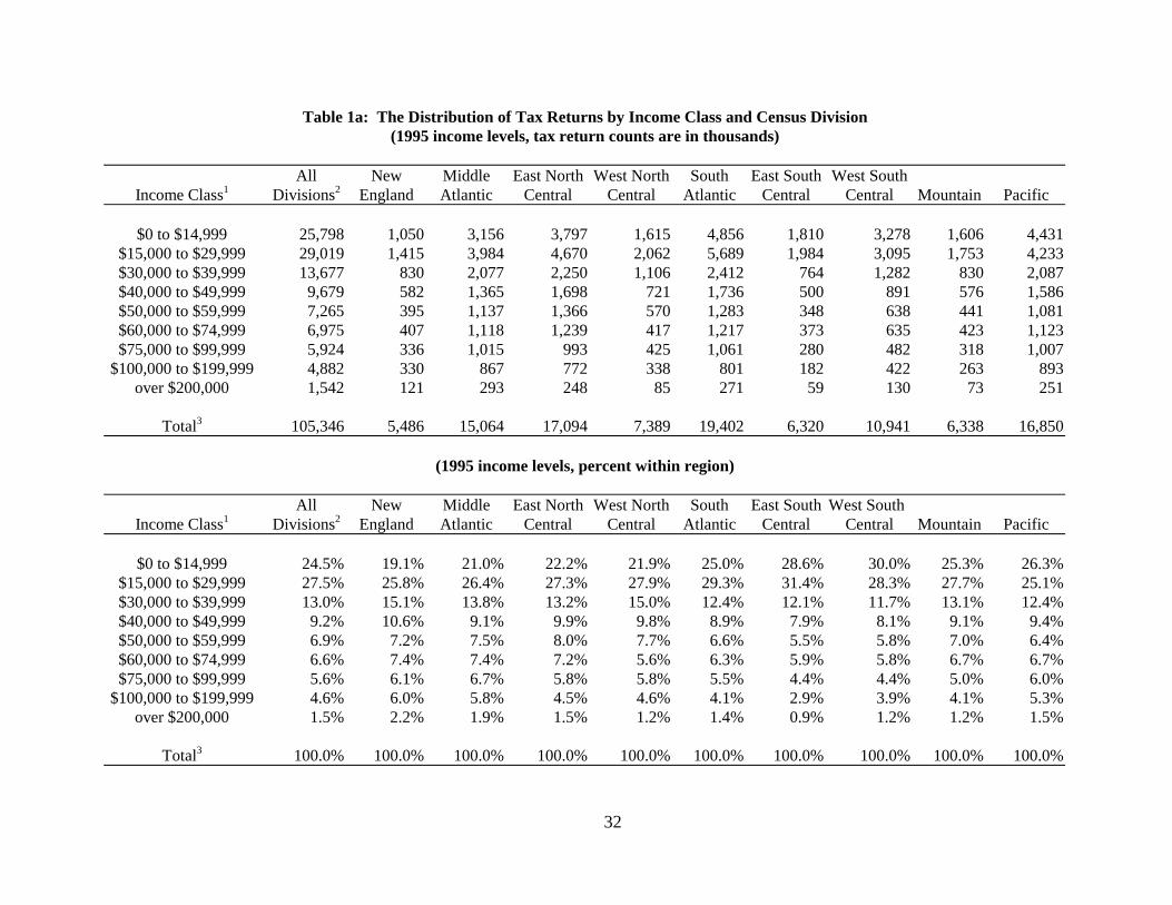
http://www.census.gov/govs/www/sttax95.html

Table 1a: The Distribution of Tax Returns by Income Class and Census Division (1995 income levels, tax return counts are in thousands)

All New Middle East North West North South East South West South Income Class1 Divisions2 England Atlantic Central Central Atlantic Central Central Mountain Pacific

$0 to $14,999 25,798 1,050 3,156 3,797 1,615 4,856 1,810 3,278 1,606 4,431 $15,000 to $29,999 29,019 1,415 3,984 4,670 2,062 5,689 1,984 3,095 1,753 4,233 $30,000 to $39,999 13,677 830 2,077 2,250 1,106 2,412 764 1,282 830 2,087 $40,000 to $49,999 9,679 582 1,365 1,698 721 1,736 500 891 576 1,586 $50,000 to $59,999 7,265 395 1,137 1,366 570 1,283 348 638 441 1,081 $60,000 to $74,999 6,975 407 1,118 1,239 417 1,217 373 635 423 1,123 $75,000 to $99,999 5,924 336 1,015 993 425 1,061 280 482 318 1,007

$100,000 to $199,999 4,882 330 867 772 338 801 182 422 263 893 over $200,000 1,542 121 293 248 85 271 59 130 73 251

Total3 105,346 5,486 15,064 17,094 7,389 19,402 6,320 10,941 6,338 16,850

(1995 income levels, percent within region)


$0 to $14,999 24.5% 19.1% 21.0% 22.2% 21.9% 25.0% 28.6% 30.0% 25.3% 26.3% $15,000 to $29,999 27.5% 25.8% 26.4% 27.3% 27.9% 29.3% 31.4% 28.3% 27.7% 25.1% $30,000 to $39,999 13.0% 15.1% 13.8% 13.2% 15.0% 12.4% 12.1% 11.7% 13.1% 12.4% $40,000 to $49,999 9.2% 10.6% 9.1% 9.9% 9.8% 8.9% 7.9% 8.1% 9.1% 9.4% $50,000 to $59,999 6.9% 7.2% 7.5% 8.0% 7.7% 6.6% 5.5% 5.8% 7.0% 6.4% $60,000 to $74,999 6.6% 7.4% 7.4% 7.2% 5.6% 6.3% 5.9% 5.8% 6.7% 6.7% $75,000 to $99,999 5.6% 6.1% 6.7% 5.8% 5.8% 5.5% 4.4% 4.4% 5.0% 6.0%

$100,000 to $199,999 4.6% 6.0% 5.8% 4.5% 4.6% 4.1% 2.9% 3.9% 4.1% 5.3% over $200,000 1.5% 2.2% 1.9% 1.5% 1.2% 1.4% 0.9% 1.2% 1.2% 1.5%

Total3 100.0% 100.0% 100.0% 100.0% 100.0% 100.0% 100.0% 100.0% 100.0% 100.0%

32

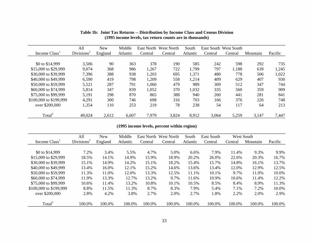
Table 1b: Joint Tax Returns -- Distribution by Income Class and Census Division (1995 income levels, tax return counts are in thousands)


$0 to $14,999 3,506 90 363 378 190 585 242 598 292 735 $15,000 to $29,999 9,074 368 986 1,267 722 1,799 797 1,188 639 1,245 $30,000 to $39,999 7,396 388 938 1,203 695 1,371 480 778 506 1,022 $40,000 to $49,999 6,590 419 798 1,209 558 1,214 409 629 407 930 $50,000 to $59,999 5,521 287 791 1,060 479 989 309 512 347 744 $60,000 to $74,999 5,814 347 839 1,052 370 1,032 335 560 359 909 $75,000 to $99,999 5,191 298 870 865 388 940 260 441 281 841

$100,000 to $199,999 4,291 300 746 698 316 703 166 376 226 748 over $200,000 1,354 110 253 219 78 238 54 117 64 213

Total3 49,024 2,612 6,607 7,979 3,824 8,912 3,064 5,259 3,147 7,447



$0 to $14,999 7.2% 3.4% 5.5% 4.7% 5.0% 6.6% 7.9% 11.4% 9.3% 9.9% $15,000 to $29,999 18.5% 14.1% 14.9% 15.9% 18.9% 20.2% 26.0% 22.6% 20.3% 16.7% $30,000 to $39,999 15.1% 14.9% 14.2% 15.1% 18.2% 15.4% 15.7% 14.8% 16.1% 13.7% $40,000 to $49,999 13.4% 16.0% 12.1% 15.2% 14.6% 13.6% 13.4% 12.0% 12.9% 12.5% $50,000 to $59,999 11.3% 11.0% 12.0% 13.3% 12.5% 11.1% 10.1% 9.7% 11.0% 10.0% $60,000 to $74,999 11.9% 13.3% 12.7% 13.2% 9.7% 11.6% 10.9% 10.6% 11.4% 12.2% $75,000 to $99,999 10.6% 11.4% 13.2% 10.8% 10.1% 10.5% 8.5% 8.4% 8.9% 11.3%

$100,000 to $199,999 8.8% 11.5% 11.3% 8.7% 8.3% 7.9% 5.4% 7.1% 7.2% 10.0% over $200,000 2.8% 4.2% 3.8% 2.7% 2.0% 2.7% 1.8% 2.2% 2.0% 2.9%

Total3 100.0% 100.0% 100.0% 100.0% 100.0% 100.0% 100.0% 100.0% 100.0% 100.0%

33

Table 1c: Single and Head of Household Tax Returns --- Distribution by Income Class and Census Division (1995 income levels, tax return counts are in thousands)


$0 to $14,999 22,292 960 2,793 3,419 1,424 4,271 1,568 2,680 1,313 3,696 $15,000 to $29,999 19,945 1,047 2,998 3,403 1,340 3,890 1,187 1,907 1,114 2,989 $30,000 to $39,999 6,280 443 1,139 1,047 411 1,041 285 505 324 1,065 $40,000 to $49,999 3,089 163 567 490 163 521 91 261 169 656 $50,000 to $59,999 1,744 108 347 306 91 294 39 126 94 338 $60,000 to $74,999 1,161 60 279 187 47 184 38 76 64 214 $75,000 to $99,999 733 38 145 128 37 121 20 41 37 166

$100,000 to $199,999 591 30 121 74 23 97 16 46 37 145 over $200,000 188 12 39 29 8 33 5 12 9 38

Total3 56,322 2,874 8,457 9,116 3,565 10,489 3,256 5,682 3,191 9,403


All New Middle East North North South East South South Income Class1 Divisions2 England Atlantic Central Central Atlantic Central Central Mountain Pacific

$0 to $14,999 39.6% 33.4% 33.0% 37.5% 39.9% 40.7% 48.2% 47.2% 41.1% 39.3% $15,000 to $29,999 35.4% 36.4% 35.4% 37.3% 37.6% 37.1% 36.5% 33.6% 34.9% 31.8% $30,000 to $39,999 11.2% 15.4% 13.5% 11.5% 11.5% 9.9% 8.8% 8.9% 10.2% 11.3% $40,000 to $49,999 5.5% 5.7% 6.7% 5.4% 4.6% 5.0% 2.8% 4.6% 5.3% 7.0% $50,000 to $59,999 3.1% 3.8% 4.1% 3.4% 2.6% 2.8% 1.2% 2.2% 2.9% 3.6% $60,000 to $74,999 2.1% 2.1% 3.3% 2.1% 1.3% 1.8% 1.2% 1.3% 2.0% 2.3% $75,000 to $99,999 1.3% 1.3% 1.7% 1.4% 1.0% 1.2% 0.6% 0.7% 1.2% 1.8%

$100,000 to $199,999 1.0% 1.0% 1.4% 0.8% 0.6% 0.9% 0.5% 0.8% 1.2% 1.5% over $200,000 0.3% 0.4% 0.5% 0.3% 0.2% 0.3% 0.2% 0.2% 0.3% 0.4%

Total3 100.0% 100.0% 100.0% 100.0% 100.0% 100.0% 100.0% 100.0% 100.0% 100.0%

34

Table 2a: The Percent of Tax Returns with Itemized Deductions by Income Class and Census Division (1995 income levels)


$0 to $14,999 3.1 4.5 4.3 2.5 1.6 3.2 1.9 2.5 2.3 4.2 $15,000 to $29,999 13.1 14.6 16.3 10.8 13.7 13.6 7.5 7.6 14.8 17.6 $30,000 to $39,999 29.1 28.0 33.2 23.9 27.3 29.4 24.3 20.9 32.0 37.3 $40,000 to $49,999 44.3 49.5 48.2 38.4 42.5 47.8 39.9 26.8 52.0 51.0 $50,000 to $59,999 59.0 66.6 66.4 57.1 57.7 59.3 49.7 45.2 63.4 60.4 $60,000 to $74,999 72.2 72.8 77.4 73.6 70.8 71.2 66.1 54.6 74.5 78.8 $75,000 to $99,999 83.4 90.2 88.0 82.3 86.7 81.7 73.6 70.0 78.3 89.0

$100,000 to $199,999 90.5 95.1 94.3 91.1 91.6 89.9 87.1 80.8 86.4 92.4 Over $200,000 91.7 98.3 97.4 90.0 97.1 90.6 83.0 79.8 93.5 92.6

Total3 31.4 37.8 38.2 30.7 31.3 30.7 22.2 20.7 31.8 35.9

Memo: Average house price ($1,000) Average state income tax rate4

Average state property tax rate4

120 2.4 3.5

163 2.9 4.7

146 3.4 4.5

102 2.9 3.8

85 2.7 3.7

105 2.2 3.2

76 1.7 1.9

77 0.7 3.1

116 2.1 3.2

178 2.4 3.3

Average age of primary 43.8 44.1 44.8 44.0 44.4 43.8 42.5 42.6 43.6 43.6 Percent filing joint 46.5 47.6 43.9 46.7 51.7 45.9 48.5 48.0 49.7 44.2 Homeownership rate (percent) 65 64 61 69 70 68 70 63 66 57

35

Table 2b: Joint Tax Returns -- Percent with Itemized Deductions by Income Class and Census Division (1995 income levels)


$0 to $14,999 $15,000 to $29,999 $30,000 to $39,999 $40,000 to $49,999 $50,000 to $59,999 $60,000 to $74,999 $75,000 to $99,999

$100,000 to $199,999 Over $200,000

Total3

6.5 15.9 7.9 4.7 3.6 7.5 7.2 4.4 4.1 8.3 14.5 16.5 23.3 13.6 10.8 14.4 7.9 7.5 12.7 22.9 26.0 26.0 30.3 19.7 21.0 27.3 19.3 18.1 30.0 38.6 42.4 52.8 47.0 33.8 41.2 45.1 38.8 25.6 50.1 52.3 58.1 66.4 67.4 56.0 58.4 58.9 47.7 44.5 64.1 58.0 71.6 73.1 75.7 74.3 67.6 70.0 65.5 56.2 75.1 78.1 83.7 90.8 87.6 85.2 87.3 82.2 74.3 70.1 75.6 88.7 91.0 95.3 93.7 92.3 91.5 90.4 86.8 82.2 88.7 92.7 92.2 98.3 97.9 90.2 97.2 91.7 82.8 79.9 94.9 93.5

47.4 57.7 57.6 47.6 44.4 46.8 35.4 32.0 45.3 54.2

Memo: Average house price ($1,000) 118 163 145 102 85 105 77 77 117 177 Average state income tax rate4 2.4 2.9 3.3 2.9 2.7 2.1 1.7 0.7 2.1 2.4 Average state property tax rate4 3.5 4.7 4.5 3.8 3.7 3.2 1.9 3.2 3.2 3.3 Average age of primary 47.5 48.1 48.9 47.6 47.6 47.8 46.1 45.9 46.7 47.3 Homeownership rate (percent) 65 65 62 69 70 68 69 63 66 57

36

Table 2c: Single and Head of Household Tax Returns --- Percent of with Itemized Deductions by Income Class and Census Division (1995 income levels)


$0 to $14,999 $15,000 to $29,999 $30,000 to $39,999 $40,000 to $49,999 $50,000 to $59,999 $60,000 to $74,999 $75,000 to $99,999

$100,000 to $199,999 over $200,000

Total3

2.6 3.4 3.8 2.2 1.3 2.7 1.1 2.0 2.0 3.3 12.5 13.9 14.0 9.8 15.2 13.2 7.3 7.7 16.0 15.4 32.7 29.8 35.6 28.8 38.1 32.2 32.7 25.3 35.0 36.0 48.2 41.0 49.8 49.8 46.8 54.1 44.9 29.7 56.5 49.2 61.7 67.0 64.3 61.0 53.8 60.7 65.6 48.2 60.7 65.6 75.2 71.1 82.3 69.7 95.5 78.1 70.8 42.7 70.9 81.9 81.2 85.1 90.5 62.5 80.2 77.9 64.8 68.9 99.0 90.2 87.1 93.9 97.7 79.3 93.1 85.6 89.6 69.3 72.3 90.8 88.0 98.2 93.9 88.1 96.1 83.2 84.2 79.5 83.9 87.9

17.6 19.7 23.1 15.8 17.1 17.0 9.9 10.2 18.6 21.5

Memo: Average house price ($1,000) 122 164 148 103 85 106 75 78 117 178 Average state income tax rate4 2.4 2.9 3.5 2.9 2.6 2.1 1.6 0.7 2.0 2.4 Average state property tax rate4 3.5 4.7 4.5 3.8 3.7 3.2 1.9 3.2 3.2 3.3 Average age of primary 40.5 40.4 41.6 40.8 40.9 40.3 39.1 39.6 40.5 40.6 Homeownership rate (percent) 64 64 61 69 70 67 69 63 65 57

37

Table 3a: Average Home Mortgage Interest Deduction (MID), Average Tax Saving, and Average Effective Subsidy Rate Conditional onMID>0

(1995 income levels)

All Divisions2 New England Mid Atlantic East North Central West North Central Income Class1 Average Tax Sub- Average Tax Sub- Average Tax Sub- Average Tax Sub- Average Tax Sub-

MID Savings sidy MID Savings sidy MID Savings sidy MID Savings sidy MID Savings sidy ($) ($) Rate ($) ($) Rate ($) ($) Rate ($) ($) Rate ($) ($) Rate

$0 to $49,999 5,609 609 10.9 5,484 624 11.4 5,198 613 11.8 4,599 494 10.7 4,501 483 10.7 $50,000 to $74,999 6,386 1,197 18.7 6,347 1,259 19.8 5,934 1,198 20.2 5,234 970 18.5 5,376 970 18.0 $75,000 to $99,999 7,745 1,992 25.7 7,547 2,043 27.1 6,740 1,817 27.0 6,490 1,707 26.3 5,840 1,532 26.2

$100,000 to $199,999 10,356 2,975 28.7 10,435 3,067 29.4 9,261 2,715 29.3 8,750 2,537 29.0 7,927 2,312 29.2 $200,000 and above 17,828 6,349 35.6 17,879 6,574 36.8 17,916 6,529 36.4 14,438 5,217 36.1 13,551 4,937 36.4

Total3 7,300 1,532 21.0 7,438 1,692 22.7 6,891 1,576 22.9 6,056 1,302 21.5 5,693 1,167 20.5

Memo:Percent of returns 26.4 31.5 28.1 26.3 25.9with MID>0

South Atlantic East South Central West South Central Mountain Pacific Income Class1 Average Tax Sub- Average Tax Sub- Average Tax Sub- Average Tax Sub- Average Tax

MID Savings sidy MID Savings sidy MID Savings sidy MID Savings sidy MID Savings ($) ($) Rate ($) ($) Rate ($) ($) Rate ($) ($) Rate ($) ($)

Sub-sidy Rate

$0 to $49,999 5,336 567 10.6 4,576 421 9.2 4,841 461 9.5 5,723 616 10.8 7,738 851 11.0 $50,000 to $74,999 6,513 1,192 18.3 5,588 924 16.5 5,118 788 15.4 6,882 1,201 17.5 8,912 1,761 19.8 $75,000 to $99,999 8,155 2,050 25.1 6,478 1,419 21.9 6,549 1,439 22.0 7,553 1,879 24.9 11,035 2,888 26.2

$100,000 to $199,999 10,700 3,069 28.7 8,665 2,332 26.9 9,690 2,610 26.9 10,326 2,896 28.0 13,860 4,004 28.9 $200,000 and above 17,795 6,252 35.1 14,503 4,919 33.9 15,193 5,039 33.2 15,849 5,522 34.8 24,351 8,642 35.5

Total3 7,193 1,463 20.3 5,936 1,073 18.1 6,426 1,251 19.5 7,150 1,349 18.9 10,047 2,110 21.0

Memo:Percent of returns 25.8 18.2 16.4 27.0 29.4with MID>0

38

Table 3b: Joint Filers' Average Home Mortgage Interest Deduction (MID), Average Tax Saving and Average Effective Subsidy RateConditional on MID>0

(1995 income levels)All Divisions2 New England Mid-Atlantic East North Central West North Central

Income Class1 Average Tax Sub- Average Tax Sub- Average Tax Sub- Average Tax Sub- Average Tax Sub-MID Savings sidy MID Savings sidy MID Savings sidy MID Savings sidy MID Savings sidy ($) ($) Rate ($) ($) Rate ($) ($) Rate ($) ($) Rate ($) ($) Rate

$0 to $49,999 6,177 538 8.7 6,151 590 9.6 5,962 578 9.7 4,816 384 8.0 4,859 378 7.8 $50,000 to $74,999 6,452 1,126 17.4 6,501 1,215 18.7 5,969 1,112 18.6 5,382 936 17.4 5,524 951 17.2 $75,000 to $99,999 7,695 1,957 25.4 7,633 2,056 26.9 6,679 1,781 26.7 6,443 1,678 26.0 5,782 1,506 26.0

$100,000 to $199,999 10,357 2,962 28.6 10,570 3,098 29.3 9,267 2,701 29.1 8,770 2,540 29.0 7,939 2,309 29.1 $200,000 and above 17,939 6,399 35.7 18,110 6,663 36.8 18,232 6,664 36.6 14,357 5,199 36.2 13,790 5,018 36.4

Total3 7,823 1,675 21.4 8,095 1,885 23.3 7,434 1,730 23.3 6,458 1,427 22.1 6,089 1,274 20.9 Memo:Percent of returns 42.3 52.0 48.6 42.9 39.4with MID>0

South Atlantic East South Central West South Central Mountain Pacific Income Class1 Average Tax Sub- Average Tax Sub- Average Tax Sub- Average Tax Sub- Average

MID Savings sidy MID Savings sidy MID Savings sidy MID Savings sidy MID ($) ($) Rate ($) ($) Rate ($) ($) Rate ($) ($) Rate ($)

Tax Savings

($)

Sub-sidy Rate

$0 to $49,999 6,001 514 8.6 4,883 356 7.3 5,046 406 8.0 6,210 536 8.6 8,506 761 8.9 $50,000 to $74,999 6,524 1,110 17.0 5,654 898 15.9 5,205 763 14.7 6,895 1,098 15.9 9,110 1,673 18.4 $75,000 to $99,999 8,201 2,046 24.9 6,511 1,414 21.7 6,524 1,421 21.8 7,849 1,935 24.7 10,922 2,819 25.8

$100,000 to $199,999 10,754 3,069 28.5 8,651 2,326 26.9 9,730 2,597 26.7 10,507 2,908 27.7 13,926 4,003 28.7 $200,000 and above 18,034 6,340 35.2 14,398 4,890 34.0 15,262 5,080 33.3 15,646 5,482 35.0 24,604 8,735 35.5

Total3 7,846 1,632 20.8 6,269 1,147 18.3 6,813 1,374 20.2 7,665 1,454 19.0 10,831 2,310 21.3 Memo:Percent of returns 42.5 31.2 27.6 41.2 49.9with MID>0

39

Table 3c: Single and Head of Household Filers' Average Home Mortgage Interest Deduction (MID), Average Tax Saving and AverageEffective Subsidy Rate Conditional on MID>0

(1995 income levels)All Divisions2 New England Mid-Atlantic East North Central West North Central

Income Class1 Average Tax Sub- Average Tax Sub- Average Tax Sub- Average Tax Sub- Average Tax Sub-MID Savings sidy MID Savings sidy MID Savings sidy MID Savings sidy MID Savings sidy ($) ($) Rate ($) ($) Rate ($) ($) Rate ($) ($) Rate ($) ($) Rate

$0 to $49,999 4,966 688 13.9 4,610 667 14.5 4,389 651 14.8 4,388 601 13.7 4,078 607 14.9 $50,000 to $74,999 6,063 1,545 25.5 5,608 1,471 26.2 5,804 1,526 26.3 4,485 1,142 25.5 4,191 1,119 26.7 $75,000 to $99,999 8,289 2,368 28.6 6,345 1,869 29.5 7,265 2,128 29.3 7,062 2,068 29.3 6,820 1,980 29.0 $100,000 to $199,999 10,340 3,130 30.3 8,786 2,675 30.4 9,198 2,855 31.0 8,397 2,483 29.6 7,682 2,372 30.9 $200,000 and above 16,675 5,832 35.0 14,450 5,263 36.4 15,238 5,382 35.3 15,412 5,427 35.2 10,105 3,764 37.2 Total3 5,764 1,113 19.3 5,254 1,052 20.0 5,371 1,145 21.3 4,803 911 19.0 4,350 803 18.5 Memo:Percent of returns 12.5 14.2 13.5 12.0 12.5with MID>0

South Atlantic East South Central West South Central Mountain Pacific Income Class1 Average Tax Sub- Average Tax Sub- Average Tax Sub- Average Tax Sub- Average

MID Savings sidy MID Savings sidy MID Savings sidy MID Savings sidy MID ($) ($) Rate ($) ($) Rate ($) ($) Rate ($) ($) Rate ($)

Tax Savings

($)

Sub-sidy Rate

$0 to $49,999 4,593 626 13.6 4,074 528 13.0 4,618 522 11.3 5,144 712 13.8 6,852 954 13.9 $50,000 to $74,999 6,455 1,630 25.3 4,944 1,170 23.7 4,529 955 21.1 6,812 1,761 25.9 8,177 2,088 25.5 $75,000 to $99,999 7,483 2,109 28.2 5,435 1,580 29.1 6,941 1,726 24.9 5,174 1,427 27.6 11,820 3,362 28.4 $100,000 to $199,999 10,005 3,061 30.6 8,852 2,409 27.2 9,175 2,776 30.3 8,763 2,791 31.8 13,411 4,011 29.9 $200,000 and above 15,228 5,308 34.9 16,031 5,334 33.3 14,334 4,539 31.7 18,021 5,951 33.0 22,277 7,884 35.4 Total3 5,336 983 18.4 4,561 767 16.8 5,066 820 16.2 5,756 1,064 18.5 8,093 1,611 19.9 Memo:Percent of returns 12.7 7.1 7.3 15.0 15.9with MID>0

40

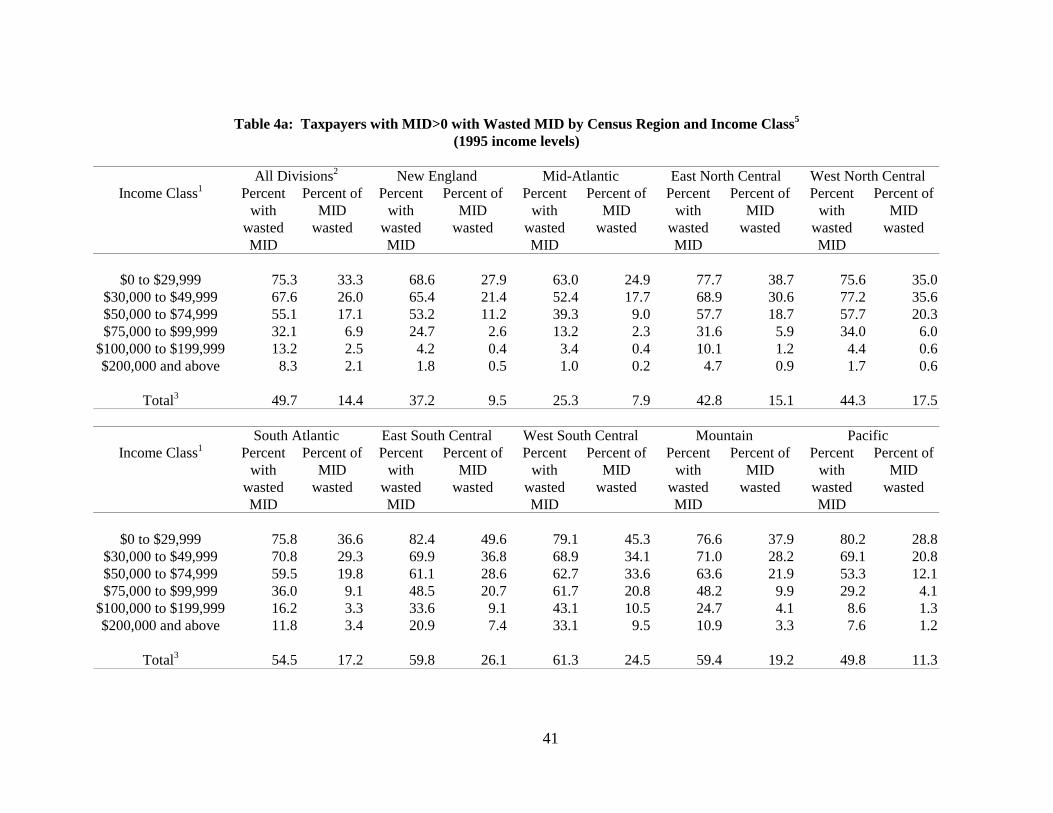
Table 4a: Taxpayers with MID>0 with Wasted MID by Census Region and Income Class5


All Divisions2 New England Mid-Atlantic East North Central West North Central Income Class1 Percent Percent of Percent Percent of Percent Percent of Percent Percent of Percent Percent of

with MID with MID with MID with MID with MID wasted wasted wasted wasted wasted wasted wasted wasted wasted wasted MID MID MID MID MID

$0 to $29,999 75.3 33.3 68.6 27.9 63.0 24.9 77.7 38.7 75.6 35.0 $30,000 to $49,999 67.6 26.0 65.4 21.4 52.4 17.7 68.9 30.6 77.2 35.6 $50,000 to $74,999 55.1 17.1 53.2 11.2 39.3 9.0 57.7 18.7 57.7 20.3 $75,000 to $99,999 32.1 6.9 24.7 2.6 13.2 2.3 31.6 5.9 34.0 6.0

$100,000 to $199,999 13.2 2.5 4.2 0.4 3.4 0.4 10.1 1.2 4.4 0.6 $200,000 and above 8.3 2.1 1.8 0.5 1.0 0.2 4.7 0.9 1.7 0.6

Total3 49.7 14.4 37.2 9.5 25.3 7.9 42.8 15.1 44.3 17.5

South Atlantic East South Central West South Central Mountain Pacific Income Class1 Percent Percent of Percent Percent of Percent Percent of Percent Percent of Percent Percent of


$0 to $29,999 75.8 36.6 82.4 49.6 79.1 45.3 76.6 37.9 80.2 28.8 $30,000 to $49,999 70.8 29.3 69.9 36.8 68.9 34.1 71.0 28.2 69.1 20.8 $50,000 to $74,999 59.5 19.8 61.1 28.6 62.7 33.6 63.6 21.9 53.3 12.1 $75,000 to $99,999 36.0 9.1 48.5 20.7 61.7 20.8 48.2 9.9 29.2 4.1

$100,000 to $199,999 16.2 3.3 33.6 9.1 43.1 10.5 24.7 4.1 8.6 1.3 $200,000 and above 11.8 3.4 20.9 7.4 33.1 9.5 10.9 3.3 7.6 1.2

Total3 54.5 17.2 59.8 26.1 61.3 24.5 59.4 19.2 49.8 11.3

41

Table 4b: Joint Tax Returns with MID > 0 with Wasted MID by Census Region and Income Class5




$0 to $29,999 75.5 36.0 68.5 29.0 70.3 28.6 78.1 44.7 71.3 38.8 $30,000 to $49,999 73.6 31.1 74.4 26.9 63.5 22.6 74.1 37.6 81.4 42.8 $50,000 to $74,999 60.8 19.1 62.6 13.0 46.6 10.7 61.7 20.3 62.7 21.7 $75,000 to $99,999 33.7 7.3 26.5 2.8 14.1 2.5 33.5 6.4 35.3 6.2

$100,000 to $199,999 13.6 2.6 3.1 0.4 3.7 0.4 10.3 1.2 4.6 0.6 $200,000 and above 8.5 2.1 1.6 0.5 1.1 0.2 4.7 0.9 1.1 0.6

Total3 48.9 14.2 44.3 9.4 33.9 7.9 47.7 14.2 50.2 17.0



$0 to $29,999 70.5 35.6 84.2 53.4 75.4 41.8 72.6 42.4 82.7 32.9 $30,000 to $49,999 76.3 34.1 73.4 42.9 67.9 38.6 70.4 31.7 77.0 25.8 $50,000 to $74,999 64.8 21.7 63.0 29.6 62.1 34.7 69.4 24.8 61.8 13.9 $75,000 to $99,999 38.9 6.2 49.4 21.1 60.6 21.3 51.2 10.2 31.8 4.3 $100,000 to $199,999 16.3 0.6 35.6 9.6 45.3 11.0 26.1 4.3 9.0 1.3 $200,000 and above 11.8 0.6 21.2 7.5 33.4 9.4 9.9 2.8 8.4 1.3

Total3 52.8 16.6 59.4 26.4 58.9 23.7 58.8 19.2 49.9 11.3

42

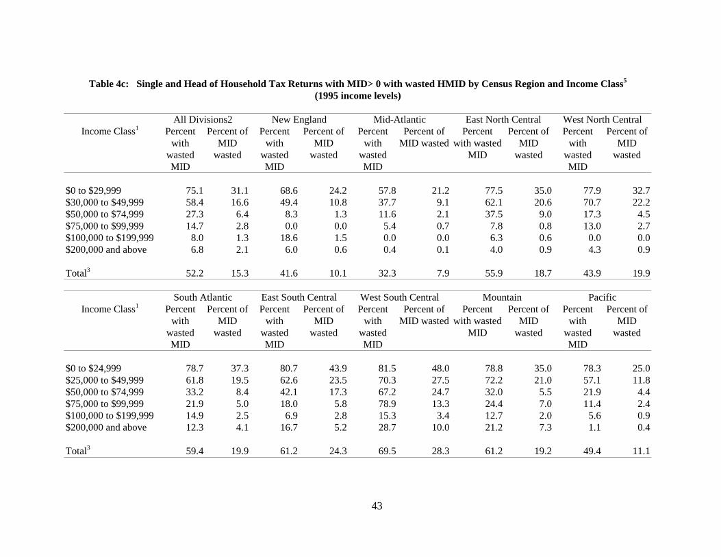
Table 4c: Single and Head of Household Tax Returns with MID> 0 with wasted HMID by Census Region and Income Class5



with MID with MID with MID wasted with wasted MID with MID wasted wasted wasted wasted wasted MID wasted wasted wasted MID MID MID MID


Total3 52.2 15.3 41.6 10.1 32.3 7.9 55.9 18.7 43.9 19.9


with MID with MID with MID wasted with wasted MID with MID wasted wasted wasted wasted wasted MID wasted wasted wasted MID MID MID MID


Total3 59.4 19.9 61.2 24.3 69.5 28.3 61.2 19.2 49.4 11.1

43

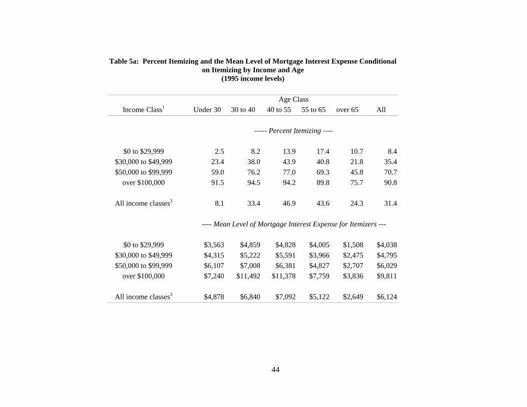
Table 5a: Percent Itemizing and the Mean Level of Mortgage Interest Expense Conditionalon Itemizing by Income and Age


Age Class Income Class1 Under 30 30 to 40 40 to 55 55 to 65 over 65 All

----- Percent Itemizing ----

$0 to $29,999 2.5 8.2 13.9 17.4 10.7 $30,000 to $49,999 23.4 38.0 43.9 40.8 21.8 35.4 $50,000 to $99,999 59.0 76.2 77.0 69.3 45.8 70.7

over $100,000 91.5 94.5 94.2 89.8 75.7 90.8

All income classes3 8.1 33.4 46.9 43.6 24.3 31.4

---- Mean Level of Mortgage Interest Expense for Itemizers ---

$0 to $29,999 $3,563 $4,859 $4,828 $4,005 $1,508 $4,038 $30,000 to $49,999 $4,315 $5,222 $5,591 $3,966 $2,475 $4,795 $50,000 to $99,999 $6,107 $7,008 $6,381 $4,827 $2,707 $6,029

over $100,000 $7,240 $11,492 $11,378 $7,759 $3,836 $9,811

All income classes3 $4,878 $6,840 $7,092 $5,122 $2,649 $6,124

44

8.4

Table 5b: Percent Itemizing and the Mean Level of Mortgage Interest Expense Conditionalon Itemizing for Joint Tax Returns by Income and Age




$0 to $29,999 3.9 12.7 18.6 19.3 6.3 12.3 $30,000 to $49,999 23.5 40.3 42.7 36.4 17.6 33.7 $50,000 to $99,999 59.3 77.4 77.7 67.3 41.0 70.9

over $100,000 93.3 95.3 94.2 91.0 74.4 91.3


----- Mean Level of Mortgage Interest Expense for Itemizers----

$0 to $29,999 $5,454 $6,064 $6,136 $4,777 $2,123 $5,428 $30,000 to $49,999 $5,332 $5,922 $6,299 $4,266 $2,981 $5,433 $50,000 to $99,999 $6,584 $7,154 $6,666 $5,058 $3,359 $6,365

over $100,000 $9,050 $12,015 $11,563 $7,917 $4,072 $9,811


45

Table 5c: Percent Itemizing and the Mean Level of Mortgage Interest Expense Conditional on Itemizing for Individual and Head of Household Tax Returns by Income and Age




$0 to $29,999 2.3 6.9 12.0 16.1 12.8 $30,000 to $49,999 23.4 35.1 45.4 49.9 31.7 37.8 $50,000 to $99,999 57.8 69.4 73.8 80.2 59.5 69.9

over $100,000 86.6 89.1 93.9 79.9 80.4 87.3


----- Mean Level of Mortgage Interest Expense for Itemizers----

$0 to $29,999 $3,095 $4,172 $4,030 $3,404 $1,368 $3,337 $30,000 to $49,999 $3,080 $4,228 $4,708 $3,515 $1,814 $3,945 $50,000 to $99,999 $4,323 $6,092 $5,012 $3,783 $1,414 $4,480

Over $100,000 $2,202 $7,270 $9,644 $6,183 $3,034 $6,934


46

7.3

--

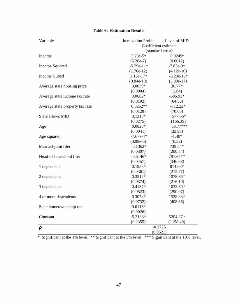
ρρρ

Table 6: Estimation Results

Variable Itemization Probit Level of MID Coefficient estimate

(standard error) Income 3.28e-5*

(6.28e-7) Income Squared -5.29e-11*

(1.76e-12)Income Cubed 2.15e-17*

(9.84e-19)Average state housing price 0.0039*

(0.0004)Average state income tax rate 0.0682*

(0.0102)Average state property tax rate 0.0262**

(0.0128)State allows MID 0.1218*

(0.0275)Age 0.0828*

(0.0041)Age squared -7.67e-4*

(3.99e-5)Married-joint filer -0.1362*

(0.0307)Head-of-household filer -0.5146*

(0.0457)1 dependent 0.1953*

(0.0361)2 dependents 0.3512*

(0.0374)3 dependents 0.4187*

(0.0523)4 or more dependents 0.3078*

(0.0732)State homeownership rate 0.0113*

(0.0026)Constant -5.2183*

(0.2355)

0.0249* (0.0012) -7.83e-9* (4.12e-10) -5.23e-16* (3.08e-17) 30.77* (1.84)

-685.93* (64.55) -712.22* (78.65) 577.66* (166.39) 63.77*** (33.98) -1.40* (0.32)

738.54* (200.54) 797.64** (346.68) 814.68* (215.77) 1078.35* (216.10) 1032.80* (290.97) 1528.88* (408.36)

5204.27* (1158.49)

ρ -0.3725 (0.0521)

* Significant at the 1% level. ** Significant at the 5% level. *** Significant at the 10% level.

47

Table 7: Importance of House Prices and State Taxes in Explaining Regional Variation in Itemization

Region All New Middle East North West North South East South West South Mountain Pacific Divisions2 England Atlantic Central Central Atlantic Central Central

Actual 31.8 37.8 38.5 31.4 31.3 31.0 22.5 20.8 31.8 35.9 Predicted 30.7 38.7 36.7 31.2 30.9 28.4 22.3 20.7 29.7 35.0

Predicted with Variables Set to Sample Average: House Price 30.6 34.4 34.0 32.9 34.2 29.6 26.9 24.0 29.9 29.7 House Price and State Taxes 30.5 33.9 32.2 32.5 32.4 29.9 27.6 27.2 29.7 29.1 Memo: Average house price ($1,000) 120 163 Average state income tax rate4 2.4 2.9 Average state property tax rate4 3.5 4.7

146 3.4 4.5

102 2.9 3.8

85 105 2.7 2.2 3.7 3.2

76 1.7 1.9

77 0.7 3.1

116 2.1 3.2

178 2.4 3.3

Summary Statistics

Variance of Percent Itemizing Across Regions

Percent of Predicted Regional Variance Explained by Variables

Actual 17.5 Predicted 17.2

Predicted with Variables Set to Sample Average: House Price 10.2 House Price 40.7 House Price and State Taxes 6.7 House Price and State Taxes 61.3

48

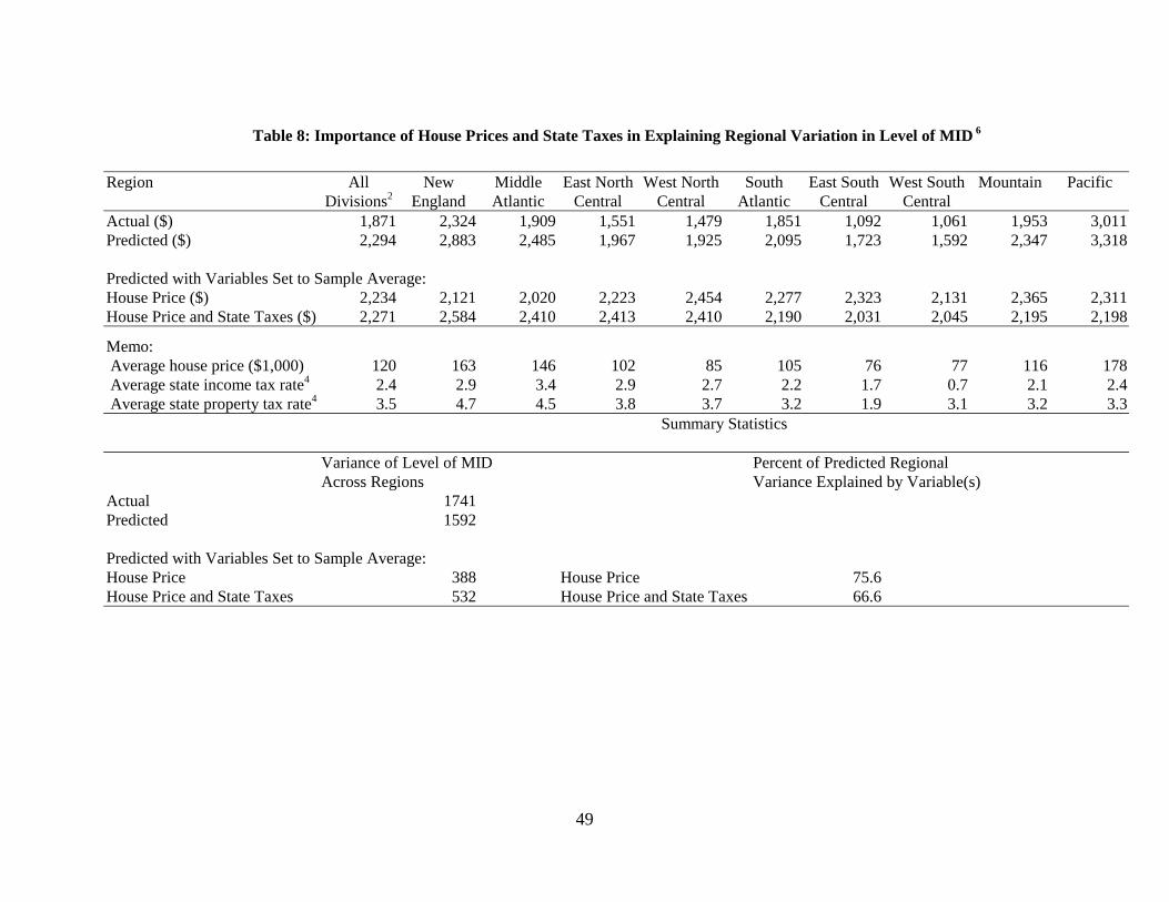
Table 8: Importance of House Prices and State Taxes in Explaining Regional Variation in Level of MID 6

Region All New Middle East North West North South East South West South Mountain Pacific Divisions2 England Atlantic Central Central Atlantic Central Central

Actual ($) 1,871 2,324 1,909 1,551 1,479 1,851 1,092 1,061 1,953 3,011 Predicted ($) 2,294 2,883 2,485 1,967 1,925 2,095 1,723 1,592 2,347 3,318

Predicted with Variables Set to Sample Average: House Price ($) 2,234 2,121 2,020 2,223 2,454 2,277 2,323 2,131 2,365 2,311 House Price and State Taxes ($) 2,271 2,584 2,410 2,413 2,410 2,190 2,031 2,045 2,195 2,198

Memo: Average house price ($1,000) 120 163 Average state income tax rate4 2.4 2.9 Average state property tax rate4 3.5 4.7

146 3.4 4.5

102 2.9 3.8

85 2.7 3.7

105 2.2 3.2

76 1.7 1.9

77 0.7 3.1

116 2.1 3.2

178 2.4 3.3

Summary Statistics

Variance of Level of MID Across Regions

Percent of Predicted Regional Variance Explained by Variable(s)

Actual 1741 Predicted 1592

Predicted with Variables Set to Sample Average: House Price 388 House Price 75.6 House Price and State Taxes 532 House Price and State Taxes 66.6

49

Table Footnotes:

(1) Income is "total income" (1040 definition) plus: tax exempt interest, nontaxable pension and social security benefits, and deferred wages (including 401k contributions) of the primary and/or spouse.

(2) The "All Divisions" column includes taxpayers who reside outside the 50 United States. New England: Maine, New Hampshire, Vermont, Massachusetts, Rhode Island and Connecticut. Middle Atlantic: New York, New Jersey, and Pennsylvania. East North Central: Ohio, Indiana, Illinois, Michigan, and Wisconsin. West North Central: Minnesota, Iowa, Missouri, North Dakota, South Dakota, Nebraska, and Kansas. South Atlantic: Delaware, Maryland, District of Columbia, Virginia, West Virginia, North Carolina, South Carolina, Georgia, and

Florida. East South Central: Kentucky, Tennessee, Alabama, and Mississippi. West South Central: Arkansas, Louisiana, Oklahoma, and Texas. Mountain: Montana, Idaho, Wyoming, Colorado, New Mexico, Arizona, Utah, and Nevada. Pacific: Washington, Oregon, California, Alaska, and Hawaii.

(3) The total line includes taxpayers with negative incomes.

(4) Total state and local taxes divided as a percent of state income as reported by Department of Census.

(5) Wasted deductions are defined as max(standard deduction – non-MID itemized deductions, 0).

(6) Individuals with incomes over $500,000 excluded.

50

-- --

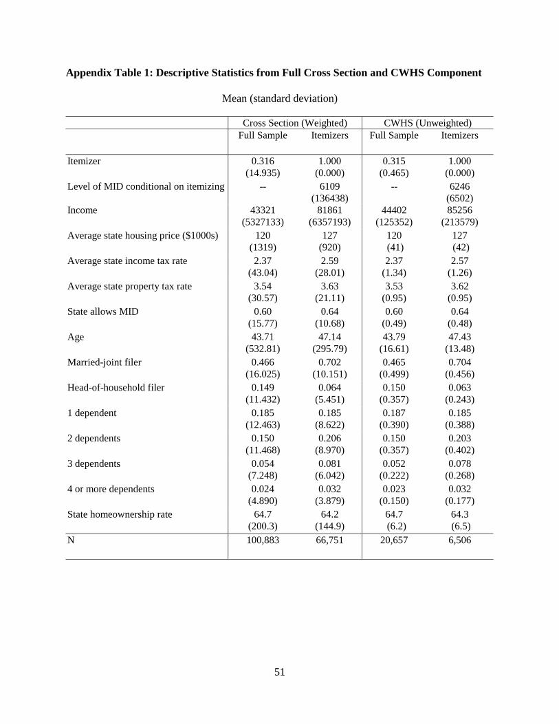
Appendix Table 1: Descriptive Statistics from Full Cross Section and CWHS Component

Mean (standard deviation)

Cross Section (Weighted) CWHS (Unweighted) Full Sample Itemizers Full Sample Itemizers

Itemizer 0.316 (14.935)

1.000 (0.000)

0.315 (0.465)

1.000 (0.000)

Level of MID conditional on itemizing 6109 (136438)

6246 (6502)

Income 43321 (5327133)

81861 (6357193)

44402 (125352)

85256 (213579)

Average state housing price ($1000s) 120 (1319)

127 (920)

120 (41)

127 (42)

Average state income tax rate 2.37 (43.04)

2.59 (28.01)

2.37 (1.34)

2.57 (1.26)

Average state property tax rate 3.54 (30.57)

3.63 (21.11)

3.53 (0.95)

3.62 (0.95)

State allows MID 0.60 (15.77)

0.64 (10.68)

0.60 (0.49)

0.64 (0.48)

Age 43.71 (532.81)

47.14 (295.79)

43.79 (16.61)

47.43 (13.48)

Married-joint filer 0.466 (16.025)

0.702 (10.151)

0.465 (0.499)

0.704 (0.456)

Head-of-household filer 0.149 (11.432)

0.064 (5.451)

0.150 (0.357)

0.063 (0.243)

1 dependent 0.185 (12.463)

0.185 (8.622)

0.187 (0.390)

0.185 (0.388)

2 dependents 0.150 (11.468)

0.206 (8.970)

0.150 (0.357)

0.203 (0.402)

3 dependents 0.054 (7.248)

0.081 (6.042)

0.052 (0.222)

0.078 (0.268)

4 or more dependents 0.024 (4.890)

0.032 (3.879)

0.023 (0.150)

0.032 (0.177)

State homeownership rate 64.7 (200.3)

64.2 (144.9)

64.7 (6.2)

64.3 (6.5)

N 100,883 66,751 20,657 6,506

51

ota paper 88 - regional differences in the utilization … · regional differences in the...

Documents