Othman, M., Cooper, J., Pirrera, A., Weaver, P., & H.C. Silva, G. (2016).Robust Aeroelastic Tailoring For Composite Aircraft Wings. 1. Paperpresented at 5th Aircraft Structural Design Conference, Manchester, UnitedKingdom.

Early version, also known as pre-print

Link to publication record in Explore Bristol ResearchPDF-document

This is the submitted manuscript. The final published version (version of record) is available online via RoyalAeronautical Society at http://dev.aerosociety.com/About-Us/Shop/Shop-Products?category=Proceedings.Please refer to any applicable terms of use of the publisher.

University of Bristol - Explore Bristol ResearchGeneral rights

This document is made available in accordance with publisher policies. Please cite only the publishedversion using the reference above. Full terms of use are available:http://www.bristol.ac.uk/pure/about/ebr-terms

Robust Aeroelastic Tailoring For Composite Aircraft Wings

Muhammad F. Othmana,1,∗, Jonathan E. Coopera,2, Alberto Pirreraa,3, Paul M. Weavera,4,Gustavo H.C. Silvab,5

aAdvanced Composites Centre for Innovation and Science, Aerospace Engineering Department, University of Bristol,Queens Building, University Walk, Bristol BS8 1TR, UK

bEmbraer S.A., Sao Jose dos Campos, Sao Paulo, 12227-901, Brazil

Abstract

An optimisation framework is presented for robust design configuration of composite aircraft wingsthrough consideration of uncertainties in material properties, ply orientations and thickness. A detailedFinite Element wing box model of a regional jet airliner is used as a benchmark. The wing structure isoptimised for minimum weight with strain, buckling, flutter/divergence and gust constraints. PolynomialChaos Expansion approach is used to efficiently quantify the effects of uncertainty in the design parameters.This method is used to determine the probability of flutter/divergence occurring, and the allowable rootbending moment being exceeded, for any given design specification which is then optimised using a ParticleSwarm Optimisation algorithm. Results are compared with deterministic solution for optimal flutter speedand minimum root bending moment. Three layup strategies were undertaken, a first which only consists of0, ±45 and 90 plies, a second which included ±30 and ±60 plies and a third which also uses ±15 and±75 plies. A minimum improvement in reliability of 32.6% is achieved for laminate with 0, ±45 and 90

plies and highest reduction in mean root bending moment value is obtained with inclusion of ±30 and ±60

plies. The layup strategy with 0, ±30, ±45, ±60 and 90 plies give the optimal robust solution for bothflutter and root bending moment responses.

Keywords: Composite structures, Aeroelastic Tailoring, Multi-constraint optimisation, Robustoptimisation, Polynomial Chaos Expansion, Flutter, Gust alleviation, Lamination parameters

1. Introduction

There is currently a lot of interest in the useof composite materials for aircraft structural design.Although the possibility of aeroelastic tailoring hasbeen around since the early 1980s, most applica-tions of carbon fibre reinforced polymer (CFRP) havebeen “black metal” designs which do not exploit theanisotropic properties. One possible reason for thedelays in designing aeroelastically tailored aircraftstructures is the explosion in the number of designvariables that occur.

Aeroelastic tailoring is defined as the process ofembodiment of the directional stiffness on the wingstructure in order to control the aerodynamic defor-mation, both static and dynamic [1]. The aim foraeroelastic tailoring is to obtain minimum structuralweight with improvement in aeroelastic and struc-tural performance of the wing. This can be achieved

by modifying the design of bending and torsional cou-pling of the composite structure by means of materialtailoring or structural tailoring.

Recent works on aeroelastic tailoring of compositewings have focused on the optimisation of the wingstructure subjected to multiple constraints includingstress [2, 3], strain [4], buckling [5], aeroelastic re-sponse [2, 6, 7, 8, 9], gust alleviation [7, 4] and aileroneffectiveness [5]. Weight minimisation is solely themain objective in aeroelastic tailoring. Weight sav-ing was able to be achieved without compromisingthe performance contraints of the wing. Other workson aeroelastic tailoring have been focused on multi-level optimisation of the composite wing [10, 4, 8].Because of high computational costs involved whendealing with detailed finite element models, multi-level or multi-stage optimisation approaches providea good alternative for aeroelastic tailoring. Multi-

∗Corresponding authorEmail address: muhammad.othman@bristol.ac.uk (Muhammad F. Othman)

1PhD Student.2RAEng Airbus Sir George White Professor of Aerospace Engineering. AFAIAA.3Lecturer in Aerospace Engineering.4Professor in Lightweight Structures.5Tehnology Development Engineer.

level optimisation provides a platform for possibilityof improving computational efficiency by reducing thenumber of design variables required from one level toanother as well as to separate different types of anal-ysis within each level.

A further consideration in aeroelastic tailoring isthe effect of uncertainty on the entire design processwhich could be used to develop robust optimum de-signs. Uncertainty is defined as “an imperfect stateof knowledge or a variability resulting from a vari-ety of factors including, but not limited to, lack ofknowledge, applicability of information, physical vari-ation, randomness or stochastic behavior, indetermi-nacy, judgment, and approximation” [11]. “Uncer-tainty can arise as a result of incomplete information,errors in both analysis and design models, and the un-certain nature of inputs and system parameters” [12].Uncertainty in aeroelasticity and composite structurecan exist due to a number of sources including non-linearity of the structure, errors in aerodynamic pre-diction, variability in material properties such as ma-terial non-homogeneity, fibre misalignment, waviness,wrinkling and defects, as well as the manufacturingtolerance and thickness variations [13, 14].

There are a number of methods available to ad-dress uncertainties in composite structures includ-ing Monte Carlo Simulation (MCS) [15, 16], Poly-nomial Chaos Expansion (PCE) [14, 17, 13, 18] andStochastic Collocation [19]. MCS is a common andstraightforward technique used to quantify uncertain-ties. However, large computational efforts are neces-sary to produce meaningful results. MCS and pertur-bation technique methods have been used to modelflutter behavior of an aeroelastic wing with uncertainbending and torsional stiffness [20]. PCE has beenused to model uncertainties in a number of models,such as a composite lifting surface with uncertain ma-terial properties, fiber direction angles and ply thick-ness [14], and aeroelastic stability of composite platewings with uncertain ply orientations using lamina-tion parameters [13]. Ref. [13] reported on the uncer-tainties quantification for aeroelastic stability usingsimple cantilever wing model representation.

Polynomial Chaos Expansion (PCE) togetherwith lamination parameters are used for the analysiswhich resulted in greater computational efficiency ascompared to other approaches such as Monte CarloSimulation. The inclusion of uncertainty studies inaeroelastic models would be significant in order toquantify and identify a robust composite wing designwhich is insensitive to small changes in design param-eters, such as ply orientations material properties andthicknesses.

In this paper, an attempt was made to performrobust optimisation on a detailed finite element wingbox model for minimum structural weight with mul-

tiple constraints including strain, buckling, aeroelas-tic response and gust alleviation. The PolynomialChaos Expansion (PCE) model is used to quantifythe variation in material properties, ply angles andply thicknesses of a composite material. Three layupstrategies are adopted as design variables for robustoptimisation to account for ply angle variations in themodel.

2. Model Definition

A detailed Finite Element (FE) wing box modelof a regional jet airliner was used for the analysisto demonstrate the effectiveness of the method. Aswept wing configuration with aspect ratio of 10 istaken as the case study. The wing geometry andthe load carrying wing box within the planform aredepicted in Fig. 1(a). The dimension given is innormalised form. The structural entities includingthe spars, ribs and stringers sections were defined inthe model. Three main spars and the ribs, includingthose at the root and tip are modelled and positionedequidistant in the spanwise direction aligned with theglobal x-axis. The stringers are included in the modelas bar elements. The skin, ribs and spars are definedusing composite material properties while others us-ing mass less aluminium properties.

A total of 25, 543 elements with bars and shellsrepresentation are used for the structural mesh.Both, the aerodynamic grids and the structural meshof the composite wing model are coupled together us-ing a surface spline which is used to interpolate theaerodynamic grid points to the structural mesh pointsfor aeroelastic analysis. For aerodynamic modelling,the aerodynamic panels are divided into two sections,with the outer wing having a higher mesh density ascompared to the inner wing section as shown in Fig.1(b).

3. Deterministic Optimisation

The composite wing structure was optimised forminimum structural weight with strain, buckling,flutter/divergence and gust response constraints.MSc. Nastran was used throughout the analysis.Only the top skin, bottom skin and the spar sectionsof the wing were optimised because of their effectiveinfluence to the wing structure‘s strength and stiff-ness. A total of 41 panels are modelled for the skinand spar sections as shown in Fig. 2. A penaltyfunction with weighting factors was assigned on theflutter/divergence and gust response constraints. Itis very likely that if the wing is optimised consider-ing only one of the parameter, the performance of theother constraints will be poor.

2

Figure 1: (a) Wing geometry and different mass entities in the FE model, (b) Aerodynamic grid.

Thus, the penalty function introduced should pro-vide an indication of how much the responses have aneffect on the optimal solution and is given by follow-ing equation.

ΩPenalty =(wf ×Vf − Vf,Design

Vf,Design)...

+ (wg ×RBM −RBMDesign

RBMDesign)

(1)

where Vf and Vf,Design is the flutter speed and de-sign flutter speed. RBM is the wing root bendingmoment.

Figure 2: Panel partitions used for the wing model.

For a minimum structural weight optimisation,the strain constraint is defined in terms of FailureIndex, FI, using the maximum strain criterion ac-cording to Eqn. (3). A static maneuver load case isconsidered for the analysis, with Mach number, cruisealtitude and acceleration of 0.82, 10 000 m and 2.5g, respectively. The static load for the flight condi-tion is obtained from aerostatic analysis. The upperboundary for strain Failure Index is set as 1.0. Forbuckling analysis, only the first ten buckling modeswere considered with the lower boundary of criticalload factor, λ is set as 1.0. In flutter analysis, theupper boundary set as 1.15VD, where VD is the flightdive velocity. The constraint for gust response is

set as the minimum value of wing root bending mo-ment (RBM). Explanations for the flutter and gustresponse analysis are given in detail in Sections 3.2and 3.3. The multi-constraints optimisation problemfor a minimum weight objective is expressed as fol-lows.

Min. Weight, W(X)

Strain Failure Index, FI(X) ≤ 1 (Max. Strain)

Buckling critical load factor,λ ≥ 1

Flutter speed,Vf ≥ 1.15VD (VD= Design DIVE speed)

Wing Root Bending Moment, RBM = min(RBM)

Design Variables,X = [ξ1, ..., ξ4, ξ9, ..., ξ11

and tpanel,1, ..., tpanel,41]

(2)The failure index for the strain constraints is derivedfrom the principal and shear strains as:

FI =εL

ε1,allowableand

γLTγLT,allowable

(3)

where, εL is the strain in longitudinal direction andγLT is the shear strain in the longitudinal and trans-verse directions. The allowable strain values used forthe analysis are given in Table 8.

Table 1: Strain allowable values for composite laminate.

Label Values Remarks

StrPmin -5.90E-03 Principal strain under compressionStrPmax 7.10E-03 Principal strain under tensionStrShrmax 4.50E-03 Maximum shear strainStrShrmin -4.50E-03 Minimum shear strain

For the deterministic optimisation, a total of328 design variables were defined in the optimi-sation problem with seven lamination parameters(ξ1, ξ2, ξ3, ξ4, ξ9, ξ10, ξ11) and a panel thickness pa-rameter for each of the 41 panels. The deterministicoptimisation is performed using the Particle SwarmOptimisation (PSO) algorithm with maximum itera-tion numbers of 50 and 20 particles for each iteration.

3

3.1. Composite Material Properties: Lamination Pa-rameters

In classical lamination theory [21], the in-plane(A) and out-of-plane stiffnesses (D) can be describedas

NM

=

A 00 D

εκ

(4)

where the generalised stress components are N =Nx, Ny, NxyT and M = Mx,My,MxyT . Thegeneralised strain components are given by ε =εx, εy, εxyT and κ = κx, κy, κxyT . The in-planeand out-of-plane stiffnesses are given by Aij andDij , respectively where i, j = 1, 2, ...6. The stiff-ness components, Aij and Dij can be represented byusing the stiffness invariants Ui(i = 1, 2, 3, 4, 5) andthe in-plane and out-of-plane lamination parametersξi(i = 1, 2, 3, 4, 9, 10, 11, 12) in accordance with thefollowing equation

A11

A12

A22

A66

A16

A26

= t

1 ξ1 ξ2 0 00 0 −ξ2 1 01 −ξ1 ξ2 0 00 0 −ξ2 0 1

0 ξ32 ξ4 0 0

0 ξ32 −ξ4 0 0

U1

U2

U3

U4

U5

(5)

D11

D12

D22

D66

D16

D26

=t3

12

1 ξ9 ξ10 0 00 0 −ξ10 1 01 −ξ9 ξ10 0 00 0 −ξ10 0 1

0 ξ112 ξ12 0 0

0 ξ112 −ξ12 0 0

U1

U2

U3

U4

U5

(6)

where t is the thickness of the plate. By definingthe non-dimensional though thickness coordinate de-noted by u(= 2z

t ), the lamination parameters can beexpressed in terms of ply orientation θ as

ξ1, ξ2, ξ3, ξ4 =1

2

∫ 1

−1cos 2θ(u), cos 4θ(u), ...

sin 2θ(u), sin 4θ(u)du(7)

ξ9, ξ10, ξ11, ξ12 =3

2

∫ 1

−1cos 2θ(u), cos 4θ(u), ...

sin 2θ(u), sin 4θ(u)u2du(8)

The lamination parameters are not independentand the relation of the lamination parameters can beexpressed in Eqn.(9), which defines the feasible region

for the parameters [22].

2ξ21 < ξ2 (9a)

ξ29 + ξ211 ≤ 1 (9b)

2(1 + ξ10)ξ211 − 4ξ9ξ11ξ12 + ξ212...

−(ξ10 − 2ξ29 + 1)(1− ξ10) 6 0(9c)

For example, the feasible region of (ξ9, ξ10) whenD16 = D26 = 0, i.e. (ξ11, ξ12) = (0, 0), can be ex-pressed from Eqn.(9) by following inequality expres-sion:

2ξ29 − 1 6 ξ10 6 1 (10)

The use of lamination parameters for the optimisa-tion of composite structures should reduce the num-bers of linear equations to approximately determinethe feasible region and hence requires less compu-tational efforts in optimisation processes. For bal-anced symmetric laminates, the stiffness componentin Bij = 0 and hence the value of ξ5 to ξ8 is as-sumed as zero and ξ12=0. Consequently, only sevenvariables of lamination parameter were considered asdesign variables with an additional variable for lam-inate thickness. The composite material propertiesare summarised in Table 2.

Table 2: Composite material properties (IM7 tape)[23].

Property ValuesE1 (GPa) 148.0E2 (GPa) 10.3G12 (GPa) 5.90υ12 0.27Density, ρ(kgm−3) 1580Ply thickness, tply (mm) 0.183

3.2. Aeroelastic analysis

In aeroelastic analysis, the flutter/divergenceanalysis of the composite wing model was performedon MSc Nastran using Sol. 145: Flutter analysis.The PK method was used to predict the flutter/di-vergence occurrence. The governing equation for thePK method can be described as follows [24].

[−Mhhp2 + (Bhh − 0.25ρcV QIhh(M,k)/k) + ...

(Khh − 0.5ρV 2QRhh(M,k))]uh = 0(11)

where Mhh is the modal mass, Bhh is the damping,Khh is the stiffness matrix, M , k and uh are the Machnumber, reduced frequency and modal amplitude vec-tor. QIhh and QRhh are the imaginary and real part ofthe eigenvalues, Qhh. The flutter/divergence frequen-cies and damping are obtained from the analysis asfunctions of velocity and relative model amplitudes.The corresponding critical flutter speed and diver-gence speeds can be determined via V − g and V − f

4

plots. A total of six modes were assumed for the com-posite wing model. The instability occurs when thereal part of Qhh is positive. The flutter point was de-termined when the imaginary part of the eigenvalueis non-zero and divergence occurs when the imagi-nary part of the eigenvalue is zero. The flutter pointcan be deduced from a V − g plot when the dampingequals to zero.

3.3. Gust response

Optimisation of a composite wing for gust loadalleviation has been explored by various researchers[4, 25, 26, 16]. Guo et al. [4] considered wing gustresponse in term of vertical wing tip displacementwith time domain. Atmospheric turbulence idealisedas discrete gusts or continuous turbulence is one ofthe critical criteria for aircraft design as specified byaeronautical authorities (CS-25) [27]. A ′1 − cosine′discrete gust model is governed by the following ex-pression.

wg(t) =wg02

(1− cos2πV

Lgt) (12)

where, wg0 is the peak or design gust velocity, Lg isthe gust length and V is the flight speed. The gustlength, Lg varies from 18m to 216m. For this work,the design gust velocity, wg0 is 20ms−1 and the flightspeed,V is 253ms−1. The gust response constraint forthe deterministic optimisation was evaluated in termof minimum strain energy which is governed by wingroot bending moment (RBM) against discrete gustload [14, 16]. The aeroelastic dynamic response (Sol.146) in MSc. Nastran was used to evaluate the dis-crete gust response for the wing model. The responseto a discrete gust was determined by using direct andinverse Fourier transform methods [28]. Only criti-cal gust length was considered for this work which isdefined as the maximum absolute value of the rootbending moment response.

4. Robust Optimisation

The robust optimisation for the wing structurewas performed by considering the variation in mate-rial properties, ply angle and ply thickness, tply ofthe composite material. The longitudinal, E1, andthe transverse in-plane Young‘s modulus, E2 wereassumed as the random variables with coefficient ofvariation = 0.1. The mean and standard deviation forthe random variables are given in Table 3. The Poly-nomial Chaos Expansion (PCE) method was used forstochastic modelling in uncertainties quantificationanalysis due to computational efficiency. A compar-ison with Monte Carlo Simulation results was per-formed to study the accuracy of the PCE model. In

order to account for ply angle variation in robust opti-misation, three different layup strategies are adoptedas design variables for robust analysis together withthe uncertainties parameters.

Table 3: Mean and standard deviation values for ran-dom variables of the uncertainties parameters.

E1 (GPa) E2 (GPa) Ply thickness, tply (m)

Mean, µ 148.0 10.3 1.83E-04Std Dev. σ 14.8 1.03 1.83E-06

4.1. Polynomial Chaos Expansion (PCE)

Polynomial Chaos Expansion (PCE) has beenused to describe irregularities due to uncertainty inaeroelastic models [17, 13]. The Weiner-Askey Chaosexpansion from Askey Scheme [18, 29] can be used tomodel variation for random variables. The continu-ous random variables can be modelled using differenttypes of polynomials described in [13]. A simple def-inition of PCE for any second-order random processu(θ) can be represented by the expression:

u(θ) = a0Γ0 +

∞∑1

ai1Γ1(ζi1(θ)) + ...

∞∑i1=1

i1∑i2=1

ai1i1Γ2[ζi1(θ), ζi2(θ)] + ...

∞∑i1=1

i1∑i2=1

i2∑i3=1

ai1i2i3Γ3[ζi1(θ), ζi2(θ), ζi3(θ)] + ...

(13)

where ζi1(θ)∞1 is a set of independent random vari-ables, Γp[ζi1(θ), ..., ζip(θ)] is the polynomial chaos oforder p which composed of multidimensional orthog-onal polynomials, ai1, ..., aip are the deterministic ex-pansion coefficient and θ is the random character ofthe quantity involved. If ζi1(θ)∞1 is a set of stan-dard Gaussian random variables, the Γp terms can beexpressed as multi-dimensional Hermite polynomialsgiven by [29]

Γp[ζi1(θ), ..., ζip(θ)] = (−1)n ∂ne−12ζT ζ

∂ζi1(θ),...,∂ζip(θ)e

12 ζT ζ

(14)Eqn. 14 is often written as

u(θ) =

∞∑i=0

βiψi(ζ(θ)) (15)

where there is a one-to-one correlation betweenΓp[ζi1(θ), ..., ζip(θ)] and ψi(ζ(θ)) and between βi andai1, ..., aip. In practice, Eqn. 13 is truncated to di-mension d of random variable ζ and the highest order(p) of the polynomial. The total number of expansion

5

coefficients (P + 1) is given by

P + 1 =(d+ p)!

d!p!(16)

The polynomial basis, ψi of Hermite-chaos forms acomplete orthogonal basis such that

ψi(ζ)ψj(ζ) =

∫ψi(ζ)ψj(ζ)W (ζ)dζ = ψ2

i δij (17)

where,

δij =

0 if i 6= j

1 if i 6= j(18)

and W (ζ) is the weighting function for the polyno-mial

W (ζ) =1√

(2π)ne−

12 ζT ζ (19)

The complete basis polynomials are Hermite polyno-mials in terms of Gaussian variables and are orthogo-nal with respect to the weighting function W (ζ). Todemonstrate, provided that the input random vari-ables are Gaussian continuous random variables, mul-tivariate polynomial basis is deduced by taking thetensor product of 1-D Hermite polynomials whichcorrespond to each variable. For example, a 2-Dexpansion of a 3rd order PCE model for a two-dimensional Gaussian input, ζ = ζ1, ζ2T , can bewritten as

u3rd =β0 + β1ζ1 + β2ζ2 + β3(ζ21 − 1) + ...

β4ζ1ζ2 + β5(ζ22 − 1) + β6(ζ31 − 3ζ1) + ...

β7(ζ21ζ2 − ζ2) + β8(ζ22ζ1 − ζ1) + ...

β9(ζ32 − 3ζ2)

(20)

where the βi terms are the unknown coefficients thathave to be calculated using a computed test data set.

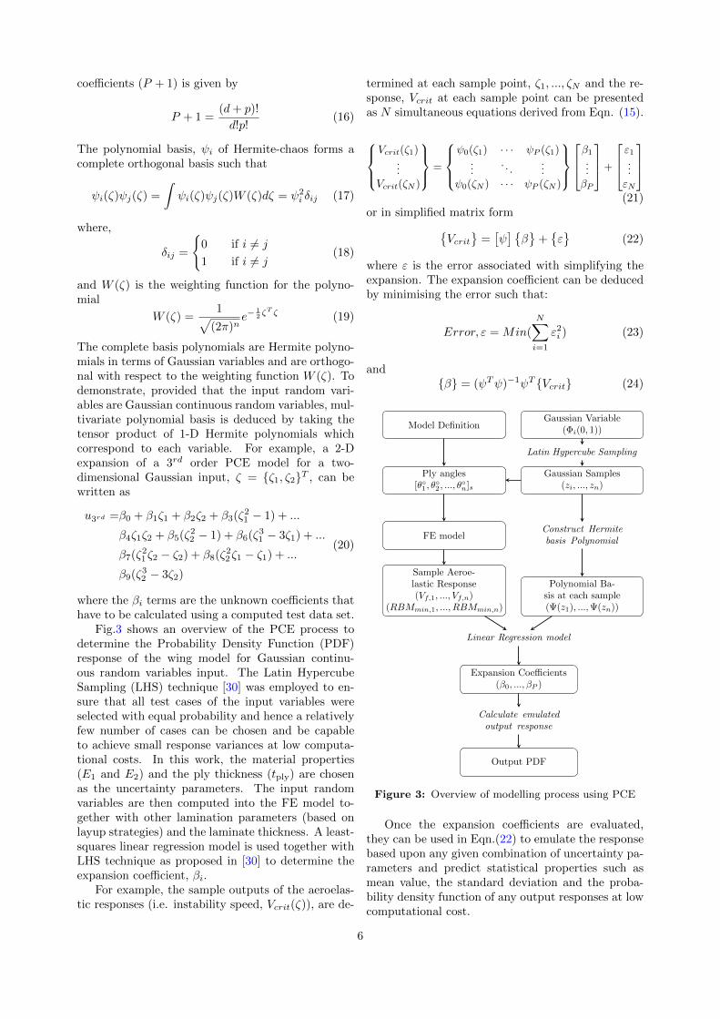
Fig.3 shows an overview of the PCE process todetermine the Probability Density Function (PDF)response of the wing model for Gaussian continu-ous random variables input. The Latin HypercubeSampling (LHS) technique [30] was employed to en-sure that all test cases of the input variables wereselected with equal probability and hence a relativelyfew number of cases can be chosen and be capableto achieve small response variances at low computa-tional costs. In this work, the material properties(E1 and E2) and the ply thickness (tply) are chosenas the uncertainty parameters. The input randomvariables are then computed into the FE model to-gether with other lamination parameters (based onlayup strategies) and the laminate thickness. A least-squares linear regression model is used together withLHS technique as proposed in [30] to determine theexpansion coefficient, βi.

For example, the sample outputs of the aeroelas-tic responses (i.e. instability speed, Vcrit(ζ)), are de-

termined at each sample point, ζ1, ..., ζN and the re-sponse, Vcrit at each sample point can be presentedas N simultaneous equations derived from Eqn. (15).

Vcrit(ζ1)

...Vcrit(ζN )

=

ψ0(ζ1) · · · ψP (ζ1)

.... . .

...ψ0(ζN ) · · · ψP (ζN )

β1...βP

+

ε1...εN

(21)

or in simplified matrix formVcrit

=[ψ] β

+ε

(22)

where ε is the error associated with simplifying theexpansion. The expansion coefficient can be deducedby minimising the error such that:

Error, ε = Min(

N∑i=1

ε2i ) (23)

andβ = (ψTψ)−1ψT Vcrit (24)

Model Definition

Ply angles[θ1 , θ

2 , ..., θ

n]s

FE model

Sample Aeroe-lastic Response(Vf,1, ..., Vf,n)

(RBMmin,1, ..., RBMmin,n)

Gaussian Variable(Φi(0, 1))

Latin Hypercube Sampling

Gaussian Samples(zi, ..., zn)

Construct Hermitebasis Polynomial

Polynomial Ba-sis at each sample(Ψ(z1), ...,Ψ(zn))

Linear Regression model

Expansion Coefficients(β0, ..., βP )

Calculate emulatedoutput response

Output PDF

Figure 3: Overview of modelling process using PCE

Once the expansion coefficients are evaluated,they can be used in Eqn.(22) to emulate the responsebased upon any given combination of uncertainty pa-rameters and predict statistical properties such asmean value, the standard deviation and the proba-bility density function of any output responses at lowcomputational cost.

6

Figure 4: PDF plots for flutter response(a) Different order of PCE model and MCS data, (b) Different number ofsamples using 3rd order PCE.

The convergence study was performed for thePCE model and compared with MCS results with5000 simulations. Figs.4(a) and 4(b) show the PDFplots for flutter response at different orders of PCEand different numbers of samples (3rd order PCE) ascompared to MCS results. It can be seen that thereis an excellent agreement with the MCS data for 1st,2nd and 3rd order PCE with 30 samples. However,the 4th order shows little discrepancy as compared toMCS data due to the limited number of samples. Thestudy on different numbers of samples for a 3rd orderPCE model shows the results starting to converge atnumber of samples = 30. Hence, it can be remarkedthat the PCE model can provide an efficient tool foruncertainties quantification with less computationalcost. The robust optimisation on this work was per-formed using a 3rd order PCE model with 30 samples.

4.2. Probabilistic Optimisation

The efficiency of PCE model to emulate the flutterand gust response of the composite wing was utilisedfor the robust design optimisation with uncertain-ties consideration. A strategy is adopted where theaeroelastic instability (flutter/divergence) occurrenceat design instability speed is minimised. Here, theconcept of maximising the reliability of the structureis used in terms of probability of survival such thatthe instability not occur before a certain design in-stability speed.

The equivalent strategy was applied for gust re-sponse except aiming to maximise the probability ofoccurence at design root bending moment (RBM) orto increase the area under the PDF plot at designvalue. Here, three layup strategies were adopted forthe design variables of robust optimisation. Only 0,±45 and 90 plies are considered in the first layup

strategy. In second layup strategy, ±30 and ±60

plies are included to account for extra design spacesfor optimisation.

Figure 5: (a) PDF plot for flutter/divergence response,(b) PDF plot for wing root bending moment(RBM).

7

The additional ±15 and ±75 plies are also in-cluded in the third layup strategy. Ply contiguityconstraint was applied to ensure no more than fourplies of a given orientation are used. For robust op-timisation, the deterministic optimal solution is firstobtained with the uncertainty parameters. The prob-ability of failure at design values are obtained andfurther minimised to obtain a robust design config-uration. Again, particle swarm optimisation (PSO)was used for the optimisation with 50 iterations and20 particles.

5. Results and discussion

5.1. Benchmark modelBased on the initial design analysis performed on

the benchmark model, the FE results show that thenormalised maximum strain is 0.4109 as shown inFig.8. Higher strain distributions are observed at thejunction of inboard and outboard wing, which arecaused by geometry change and higher stress concen-tration. The maximum failure index, FI for strain is0.3308. The minimum value for critical load factorfor the first ten buckling modes is 2.878.

Figure 6: Flutter results for the benchmark model: (a)V-f plot; (b) V-g plot

The mode shape analysis was performed on thebenchmark wing model to determine the critical vi-bration mode. The first four vibration modes and

the normalised frequency of the wing are first bend-ing (0.3683), second bending (0.5605), first torsion(0.7495) and second torsion (1.1438), respectively.

The flutter analysis results are shown in Fig.6 inthe form of V-f and V-g plots using PK method. Theresults indicate that the first bending mode coupledwith the torsion mode is the most critical one, wherethe normalised flutter speed of 0.6355 at normalisedfrequency of 0.75 was obtained when the dampingreaches zero. The flutter speed obtained is muchhigher that the normalised design flutter speed of0.3261. The gust response for the wing is measuredin term of wing root bending moment (RBM). Thecritical value is obtained at gust length of 216 m withnormalised RBM value of 4.171. The thickness vari-ation for the skin and spar section of the wing is pre-sented in Fig.7 with normalised structural weight of0.6122. The results show that the benchmark modelhas potential for weight saving by aeroelastic tailor-ing due to an ample safety margin.

Section no.

1 2 3 4 5 6 7 8

Norm

ali

sed

Th

ick

ness

0.2

0.3

0.4

0.5

0.6

0.7

0.8

0.9

1

Top skin 1Top skin 2Bottom skin 1Bottom skin 2Spar 1Spar 2Spar 3

Figure 7: Thickness variation for benchmark model.

5.2. Deterministic model

The normalised structural weight of the wingstructure was reduced to 0.5428 which is a 11.3% re-duction as compared to the benchmark wing. Theminimum weight was obtained after 20 iterations us-ing Particle Swarm optimisation (PSO) with 20 par-ticles as shown in Fig.9.

The thickness variation of the skin and spar sec-tion are presented in Fig.10. It is noticed that thick-est section is obtained at the kink area of the bottomskin panel where the stress concentration was higherdue to engine and pylon mass. A lower thicknessvalue is obtained at the tip of the top skin panel. Al-though in practice it would be more useful to includethe ply drop consideration for manufacturing compat-ibility, the results shown here provided a reasonablethickness variation for the wing model.

8

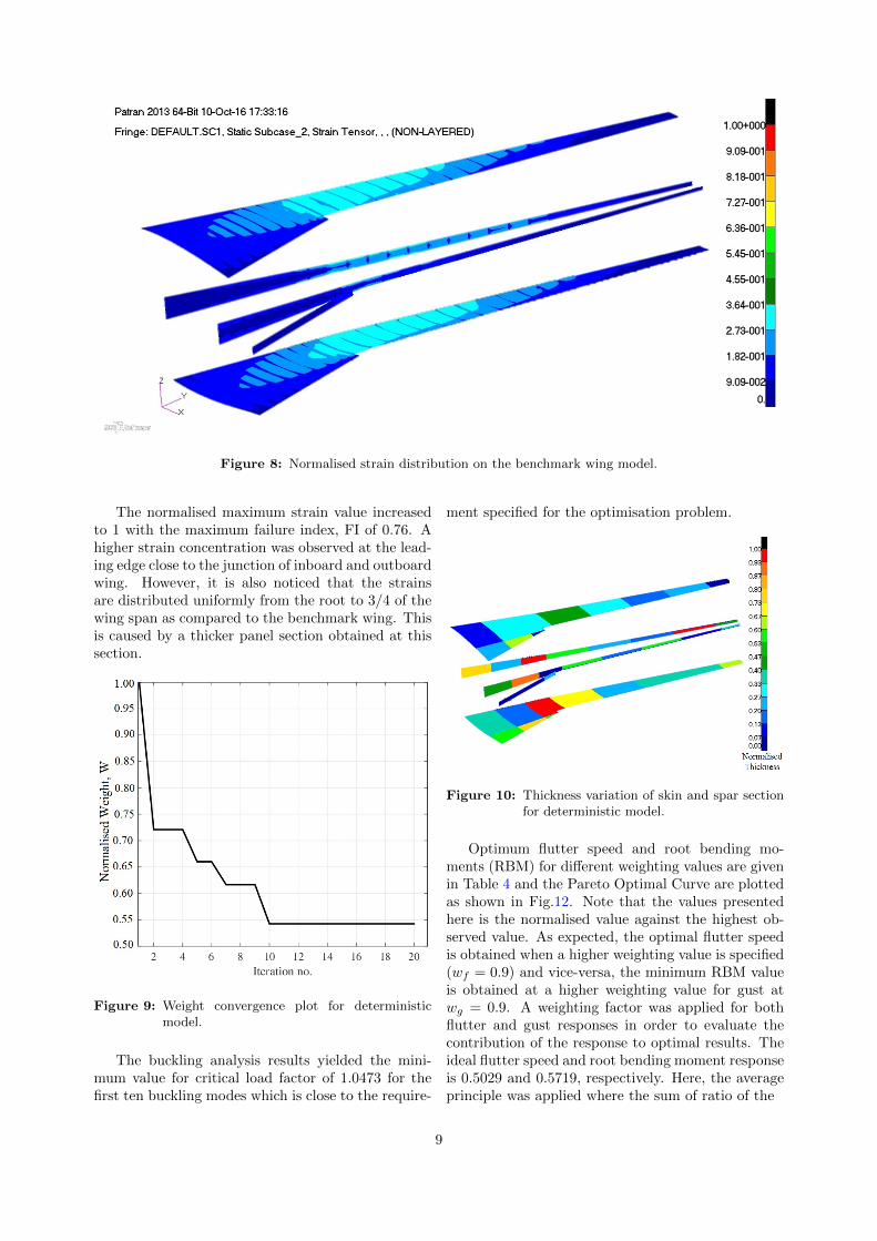
Figure 8: Normalised strain distribution on the benchmark wing model.

The normalised maximum strain value increasedto 1 with the maximum failure index, FI of 0.76. Ahigher strain concentration was observed at the lead-ing edge close to the junction of inboard and outboardwing. However, it is also noticed that the strainsare distributed uniformly from the root to 3/4 of thewing span as compared to the benchmark wing. Thisis caused by a thicker panel section obtained at thissection.

Figure 9: Weight convergence plot for deterministicmodel.

The buckling analysis results yielded the mini-mum value for critical load factor of 1.0473 for thefirst ten buckling modes which is close to the require-

ment specified for the optimisation problem.

Figure 10: Thickness variation of skin and spar sectionfor deterministic model.

Optimum flutter speed and root bending mo-ments (RBM) for different weighting values are givenin Table 4 and the Pareto Optimal Curve are plottedas shown in Fig.12. Note that the values presentedhere is the normalised value against the highest ob-served value. As expected, the optimal flutter speedis obtained when a higher weighting value is specified(wf = 0.9) and vice-versa, the minimum RBM valueis obtained at a higher weighting value for gust atwg = 0.9. A weighting factor was applied for bothflutter and gust responses in order to evaluate thecontribution of the response to optimal results. Theideal flutter speed and root bending moment responseis 0.5029 and 0.5719, respectively. Here, the averageprinciple was applied where the sum of ratio of the

9

Figure 11: Normalised strain distribution of the wing structure for optimum deterministic model.

flutter speed to the design flutter speed (1.15VD) andthe minimum RBM value to the RBM value shouldbe close to 2 for the ideal case.

Table 4: Deterministic optimisation results for flutterspeed, Vf and wing root bending moment,RBM.

Weighting Response (normalised)

wf wg Vf RBM

1.0 0.0 0.5013 3.44110.9 0.1 0.5005 2.66530.8 0.2 0.5005 1.40920.7 0.3 0.5228 1.41210.6 0.4 0.5025 0.85350.5 0.5 0.5051 0.91120.4 0.6 0.5119 1.02260.3 0.7 0.5012 0.69780.2 0.8 0.5029 0.57190.1 0.9 0.6828 0.41620.0 1.0 0.8294 0.4884

5.3. Robust optimisation

The deterministic and robust optima for the threelayup strategies at normalised design flutter speed of0.6667 and normalised design wing root bending mo-ment of 0.6429 are presented in Table 5, along withthe mean, standard deviation and probability of fail-ure for the design values. Figs. 13, 14 and 15 com-pare the Probability Density Function (PDF) for theflutter speed and RBM of the deterministic optimaas well as robust optima evaluated at design flutterspeed and design RBM values.

The mean value for the flutter speed for all layupstrategies are higher compared to the ideal flutterspeed obtained from the deterministic model due tothe variation in the longitudinal, E1, transverse in-plane Young‘s modulus, E2 and ply thickness in themodel. The probability of failure at flutter designspeed for deterministic flutter response increases asextra design space is introduced. With all layupstrategies, the robust optimisation result is consid-erably more reliable design with lower probabilitiesof failure compared to the deterministic solution.

Figure 12: Deterministic optimisation results: (a) Flut-ter speed at different weighting function, wf

plot, (b) RBM values at different weight-ing function, wg plot and (c) Flutter speedagainst RBM value plot

A 32.6% reduction in terms of the probability offailure is achieved over the laminate with only 0,

10

Table 5: Robust optimisation results for 1) 0, ±45 and 90, 2) 0, ±30, ±45, ±60 and 90 and 3) 0, ±15,±30, ±45, ±60, ±75 and 90 plies.

Layup Stategy ObjectiveFlutter speed, Vf (normalised) Root Bending Moment, RBM (normalised)

(Vf,Design = 0.6667) (RBMDesign = 0.6429)

Mean Std Dev. Probability of failure Mean Std Dev. Probability of failure

1Deterministic 0.6179 0.1643 0.008900 0.7499 0.1166 0.0023Robust 0.7126 0.1028 0.006000 0.6991 0.1238 0.0135

2Deterministic 0.7117 0.0760 0.009600 0.6193 0.1209 0.4641Robust 0.7105 0.0866 0.000529 0.3622 0.1052 1.0000

3Deterministic 0.6856 0.1829 0.031900 0.5202 0.1177 0.9851Robust 0.7196 0.0752 0.017700 0.3789 0.1359 1.0000

Figure 13: Comparison PDFs for deterministic and robust design with 0, ±45 and 90 plies: (a) Flutter response(b) RBM response.

Figure 14: Comparison PDFs for deterministic and robust design with 0, ±30, ±45, ±60 and 90 plies: (a)Flutter response (b) RBM response.

±45 and 90 plies. Higher percentage of reductionsin terms of probability of failure are achieved with theinclusion of additional plies with 94.6% and 44.8%reductions obtained for second and third layup strat-egy, respectively.

For the gust responses, the mean values for rootbending moment are reduced for all layup strategieswith the highest reduction of 41.5% obtained withthe inclusion of ±30 and ±60 plies. Figs. 14(b) and15(b) show that the PDF curves are shifted to the left

11

to accommodate for minimum value of RBM. Onlysmall improvements in terms of the RBM probabil-ity of failure are achieved for the first layup strategydue to limited design spaces. It is noteworthy thatthe PDF curve for robust flutter response using thethird layup strategy as shown in Fig. 15(a) is shiftedto the left and has a higher peak probability valueas compared to the deterministic solution. However,it also noticed that the skewness of the determinis-tic PDF curve is reduced for the robust design andthereby lowering the probability of failure at design

flutter speed.

Finally, it can be remarked that the inclusion ofextra design space in terms of the ply angles provideimprovement in reliability resulting in higher flutterspeed and lower RBM. The layup strategy with 0,±30, ±45, ±60 and 90 plies give the optimal ro-bust solution for both flutter and root bending re-sponses. Fig. 16 shows the ply configuration for op-timal robust solution with second layup strategy of[θ1θ2...θn]s where, n is the ply number.

Figure 15: Comparison PDFs for deterministic and robust design with 0, ±15, ±30, ±45, ±60, ±75 and 90

plies: (a) Flutter response (b) RBM response.

Figure 16: Ply configuration for robust design configuration with 0, ±30, ±45, ±60, and 90 plies.

12

6. Conclusion

A computationally efficient approach has beenpresented for the robust design of composite wingswith multiple constraints and uncertain materialproperties, ply orientations and ply thicknesses.Polynomial Chaos Expansion is used as a stochasticmodel for the uncertainties quantification to estimatethe Probability Density Function (PDF) and prob-ability of failure for aeroelastic and gust responses.The robust design configuration has been achievedbased on minimum probability of failure for flutter re-sponse and minimum mean value for RBM responsewhich is obtained from optimisation using the Par-ticle Swarm Optimisation algorithm. Three layupstrategies were undertaken, a first which only con-sists of 0, ±45 and 90 plies, a second which alsoincluded ±30 and ±60 plies and a third which alsouses ±15 and ±75 plies. The following observationshave been made:

• The optimal normalised weight of 0.8866 is ob-tained for a deterministic optima design whichis a 11.3% reduction from the baseline design.

• Polynomial Chaos Expansion (PCE) providessufficient accuracy for uncertainties quantifica-tion with fewer model runs (order of two magni-tude reduction) compared to Monte Carlo Sim-ulation.

• A minimum improvement in reliability of 32.6%is achieved for a laminate with 0, ±45 and 90

plies for flutter response and highest reductionin mean RBM value is obtained with the inclu-sion of ±30 and ±60 plies.

• The layup strategy with 0, ±30, ±45, ±60

and 90 plies gives the optimal robust solutionfor both flutter and root bending moment re-sponses.

It is also noted that the thickness variation obtainedfrom the optima deterministic solution has not con-sidered manufacturing constraints, such as compositeply drops, which may provide more beneficial resultsfor robust design which are subject to future work.

Acknowledgements

The authors would like to acknowledge thesupport of the EPSRC, who provide funding forthe ACCIS Centre for Doctoral Training Centre(EP/G036772/1), Embraer S.A. and also the Min-istry of Higher Education, Malaysia and UniversitySains Malaysia for the scholarship.

References

[1] M. H. Shirk, T. J. Hertz, T. Weisshaar, Aeroe-lastic tailoring — theory, practice, and promise,Journal of Aircraft 23 (1) (1986) 6–18.

[2] F. E. Eastep, V. A. Tischler, V. B. Venkayya,N. S. Khot, Aeroelastic Tailoring of Compos-ite Structures, Journal of Aircraft 36 (6) (1999)1041–1047.

[3] S. Kuzmina, V. Chedrik, F. Ishmuratov,Strength and aeroelastic structural optimizationof aircraft lifting surfaces using two-level ap-proach, 6th World Congress of Structural andMultidisciplinary Optimization.

[4] S. Guo, D. Li, Y. Liu, Multi-objective optimiza-tion of a composite wing subject to strength andaeroelastic constraints, Proceedings of the Insti-tution of Mechanical Engineers, Part G: Journalof Aerospace Engineering 226 (9) (2011) 1095–1106.

[5] J. Dillinger, T. Klimmek, M. Abdalla, Z. Gurdal,Stiffness optimization of composite wings withaeroelastic constraints, Journal of Aircraft.

[6] M. Y. Harmin, J. E. Cooper, Aeroelas-tic Tailoring Using Ant Colony Optimization,50th AIAA/ASME/ASCE/AHS/ASC Struc-tures, Structural Dynamics and Materials Con-ference, 4-7 May (May) (2009) 1–17.

[7] O. Stodieck, J. E. Cooper, P. M. Weaver,P. Kealy, Improved aeroelastic tailoring usingtow-steered composites, Composite Structures106 (2013) 703–715.

[8] Z. Wan, B. Zhang, Z. Du, C. Yang, Aeroelastictwo-level optimization for preliminary design ofwing structures considering robust constraints,Chinese Journal of Aeronautics 27 (2) (2014)259–265.

[9] N. P. M. Werter, R. D. Breuker, Aeroelastic Tai-loring and Structural Optimisation using an Ad-vanced Dynamic Aeroelastic Framework, Inter-national Forum on Aeroelasticity and StructuralDynamics (2015) 1–20.

[10] I. de Visser, Aeroelastic and strength optimiza-tion of a composite aircraft wing using a multi-level approach, Proceedings of the 40 th Struc-tures, Structural Dynamics, and Materials Con-ference and Exhibit, 1999.

[11] E. L. Walker, T. K. W. Iv, Integrated Un-certainty Quantification for Risk and ResourceManagement : Building Confidence in Design (Invited ), 53rd AIAA Aerospace Sciences Meet-ing, AIAA SciTech (January) (2015) 1–17.

13

[12] E. Livne, Future of Airplane Aeroelasticity,Journal of Aircraft 40 (6) (2003) 1066–1092.

[13] C. Scarth, J. E. Cooper, P. M. Weaver, G. H.Silva, Uncertainty quantification of aeroelasticstability of composite plate wings using lam-ination parameters, Composite Structures 116(2014) 84–93.

[14] A. Manan, J. Cooper, Uncertainty of Com-posite Wing Aeroelastic Behaviour, 12thAIAA/ISSMO Multidisciplinary Analysis andOptimization Conference.

[15] E. P. Wiser, Monte Carlo Technique with Corre-lated Random Variables 118 (2) (1992) 258–272.

[16] T.-U. Kim, I. H. Hwang, Optimal design of com-posite wing subjected to gust loads, Computers& Structures 83 (19-20) (2005) 1546–1554.

[17] G. Georgiou, A. Manan, J. Cooper, Modelingcomposite wing aeroelastic behavior with uncer-tain damage severity and material properties,Mechanical Systems and Signal Processing 32(2012) 32–43.

[18] D. Xiu, G. Em Karniadakis, Modeling uncer-tainty in steady state diffusion problems via gen-eralized polynomial chaos, Computer Methodsin Applied Mechanics and Engineering 191 (43)(2002) 4927–4948.

[19] S. Sarkar, J. A. S. Witteveen, A. Loeven, H. Bijl,Effect of uncertainty on the bifurcation behaviorof pitching airfoil stall flutter, Journal of Fluidsand Structures 25 (2) (2009) 304–320.

[20] S. C. Castravete, R. A. Ibrahim, Effect of Stiff-ness Uncertainties on the Flutter of a CantileverWing, AIAA Journal 46 (4) (2008) 925–935.

[21] H. T. Hahn, S. W. Tsai, Introduction to Com-posite Materials, Taylor & Francis, 1980.

[22] M. Kameyama, H. Fukunaga, Optimum designof composite plate wings for aeroelastic charac-teristics using lamination parameters, Comput-ers and Structures 85 (2007) 213–224.

[23] K. Marlett, Hexcel 8552 IM7 UnidirectionalPrepreg 190 gsm & 35%RC Qualification Ma-terial Property Data Report (2011) 238.

[24] E. H. Johnson, MSC Nastran Version 68 Aeroe-lastic Analysis User’s Guide - 2, Structure.

[25] S. S. Rao, Optimization of airplane wing struc-tures under taxiing loads, Computers and Struc-tures 26 (3) (1987) 469–479.

[26] S. S. Rao, L. Majumder, Optimization of Air-craft Wings for Gust Loads: Interval Analysis-Based Approach, AIAA Journal 46 (3) (2008)723–732.

[27] EASA, Certification Specifications for LargeAeroplanes, Cs-25 (September) (2008) 750.

[28] MSC Software Corporation, MSC Nastran 2012Dynamic Analysis User’s Guide, 2011.

[29] D. Xiu, G. E. Karniadakis, The Wiener–AskeyPolynomial Chaos for Stochastic DifferentialEquations, SIAM Journal on Scientific Comput-ing 24 (2) (2002) 619–644.

[30] S.-K. Choi, R. V. Grandhi, R. A. Canfield, C. L.Pettit, Polynomial Chaos Expansion with LatinHypercube Sampling for Estimating ResponseVariability, AIAA Journal 42 (6) (2004) 1191–1198.

14