Outlines:

I Earthquake statistics and the Gutenberg-Richter lawII Sandpile model and self-organized criticalityIII Other possible examples of self-organized criticalityIV Organization and dynamics of complex networks

Power Law Statistics for Earthquakes, Forest fires, Networks,

and Other Complex Systems

Kan ChenDepartment of Computational Science, NUS

Earthquake Phenomenology

It is generally believed that earthquakes result from a stick-slip dynamics involving the Earth’s crust sliding along faults. 

San-Andreas Fault marks the contact between the Pacific and North American Plates

San-Andreas fault, where the great 1906 San Francisco earthquake occurred

Earthquake PhenomenologyThe recent earthquake in Taiwan (Sept. 21, 1999) also causes

tremendous damages.

Main shock and aftershocks

The size of an earthquake is often given in term of magnitude (Richter scale), which is roughly the energy in logarithmic scale. An increase in magnitude by 1 leads to about 32-fold increase in the energy release (10-fold increase in amplitude of seismic shocks). An earthquake of magnitudes of 7

or higher typically causes tremendous damages. 

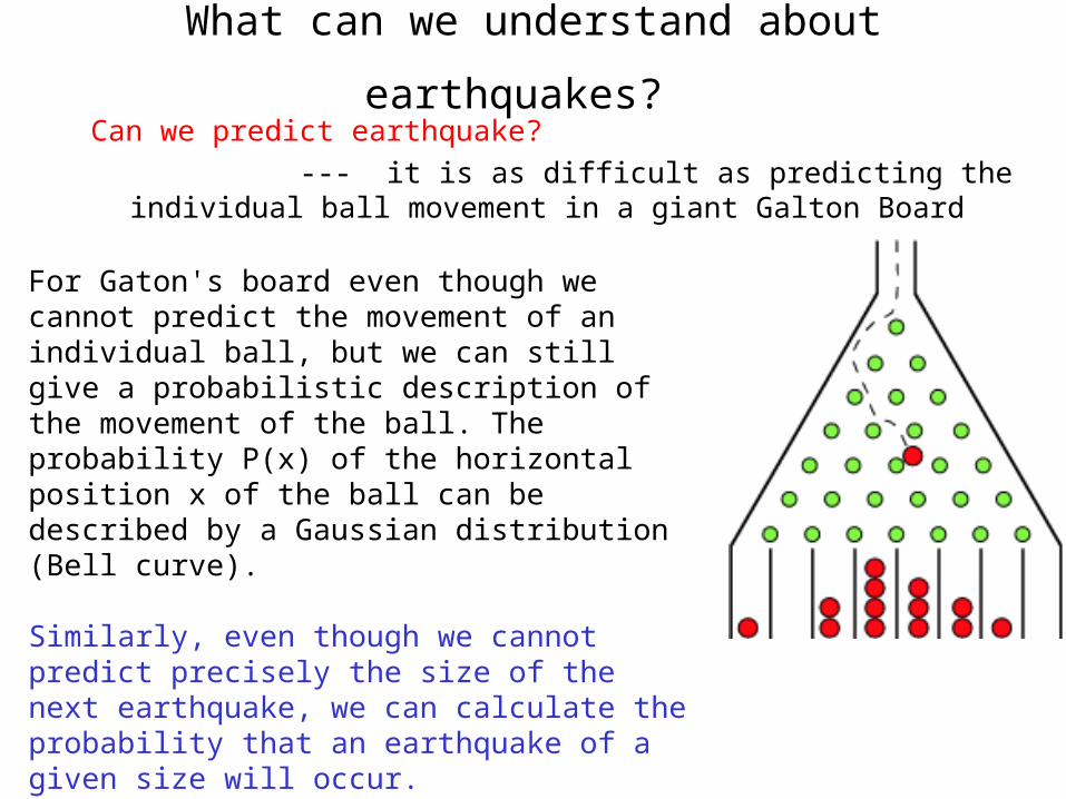
What can we understand about

earthquakes? Can we predict earthquake?            ---  it is as difficult as predicting the individual ball

movement in a giant Galton Board

For Gaton's board even though we cannot predict the movement of an individual ball, but we can still give a probabilistic description of the movement of the ball. The probability P(x) of the horizontal position x of the ball can be described by a Gaussian distribution (Bell curve).

Similarly, even though we cannot predict precisely the size of the next earthquake, we can calculate the probability that an earthquake of a given size will occur.

Gutenberg Richter LawDespite of the apparently complexity involved in the dynamics of earthquake, the probability distribution of earthquakes follows a glaringly simple distribution function known as the Gutenberg-Richter law:

The probability of having an earthquake of energy E, P(E) = c 1/E1+B,

where the exponent B is a universal exponent in the sense that it does not depend on particular geographic area. When plotted on a log-log scale, such power laws appear as straight lines, where the slope is -B:  log (P(E)) = log (c) – (1+B) log(E)

Earthquake Statistics (1995)

Gutenberg-Richter Law

There are more small earthquakes than large ones. But there is no apparent cut-off in the possible size of an earthquake; earthquakes of all sizes are possible.

If the probability distribution were of the form exp(-E/E0), then there would be a well defined cut-off at the energy E0 such that the probability for an earthquake of size E much greater than E0 is exponentially small.

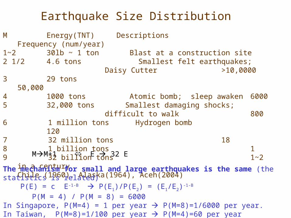
M Energy(TNT) Descriptions Frequency (num/year)

1~2 30lb ~ 1 ton Blast at a construction site 2 1/2  4.6 tons Smallest felt earthquakes;

Daisy Cutter >10,00003 29 tons 50,0004 1000 tons Atomic bomb;  sleep awaken 60005 32,000 tons Smallest damaging shocks;

difficult to walk 8006 1 million tons  Hydrogen bomb 1207 32 million tons 188 1 billion tons 19 32 billion tons 1~2 in a

centuryChile (1960), Alaska(1964), Aceh(2004)MM+1 E 32 E

The mechanism for small and large earthquakes is the same (the statistics is related)    P(E) = c  E-1-B  P(E1)/P(E2) = (E1/E2)

-1-B

P(M = 4) / P(M = 8) = 6000In Singapore, P(M=4) = 1 per year P(M=8)=1/6000 per year.In Taiwan, P(M=8)=1/100 per year P(M=4)=60 per year

Earthquake Size Distribution

Sub, Super, and Critical States

Chain reactions of dominoes

In the critical system (modelled by placing dominoes randomly on about half of the segments in a diamond grid) many sizes of chain reactions (avalanches) were produced when the dominoes in the bottom row were tipped over.

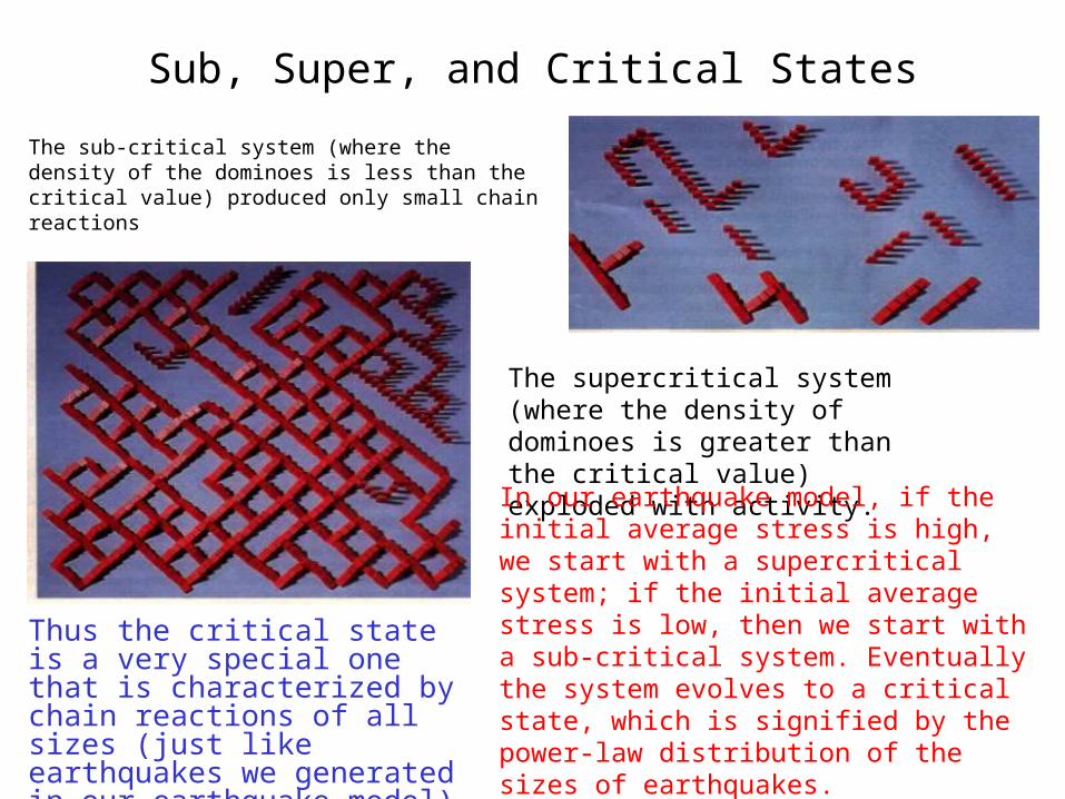
Sub, Super, and Critical States

The sub-critical system (where the density of the dominoes is less than thecritical value) produced only small chain reactions

 

Thus the critical state is a very special one that is characterized by chain reactions of all sizes (just like earthquakes we generated in our earthquake model).

The supercritical system (where the density of dominoes is greater than the critical value) exploded with activity.In our earthquake model, if the initial

average stress is high, we start with a supercritical system; if the initial average stress is low, then we start with a sub-critical system. Eventually the system evolves to a critical state, which is signified by the power-law distribution of the sizes of earthquakes.

Percolation and criticality

A simple percolation model (applet).

You may view the lattice as a forest: a given cell is either empty (with probability 1 - p) or is occupied by a tree (with probability p); p is the density of the trees in the forest.

We ask the question, if we start a fire on the left-edge of the forest, what is the probability that the fire will reach (percolate to) the right-edge?

How does the percolation probability depend on the density of the forest p.

Sand Pile and Self-organized CriticalityWhy and how do complex systems, such as the earth’s crust

(where earthquakes occur), evolve to such critical states?To answer this question, it is better to study much simpler

systems, then generalize our understanding of simple model systems to realistic complex systems --- This is the approach we adopt in our study of science of complexity. We hope to be able to understand universal properties such the Gutenberg-Richter laws exhibited in earthquake statistics.   

A deceptively simple system serves as a paradigm for self-organized criticality: a pile of sand. 

Artwork by Elaine Wiesenfeld (from Bak, How Nature Works)

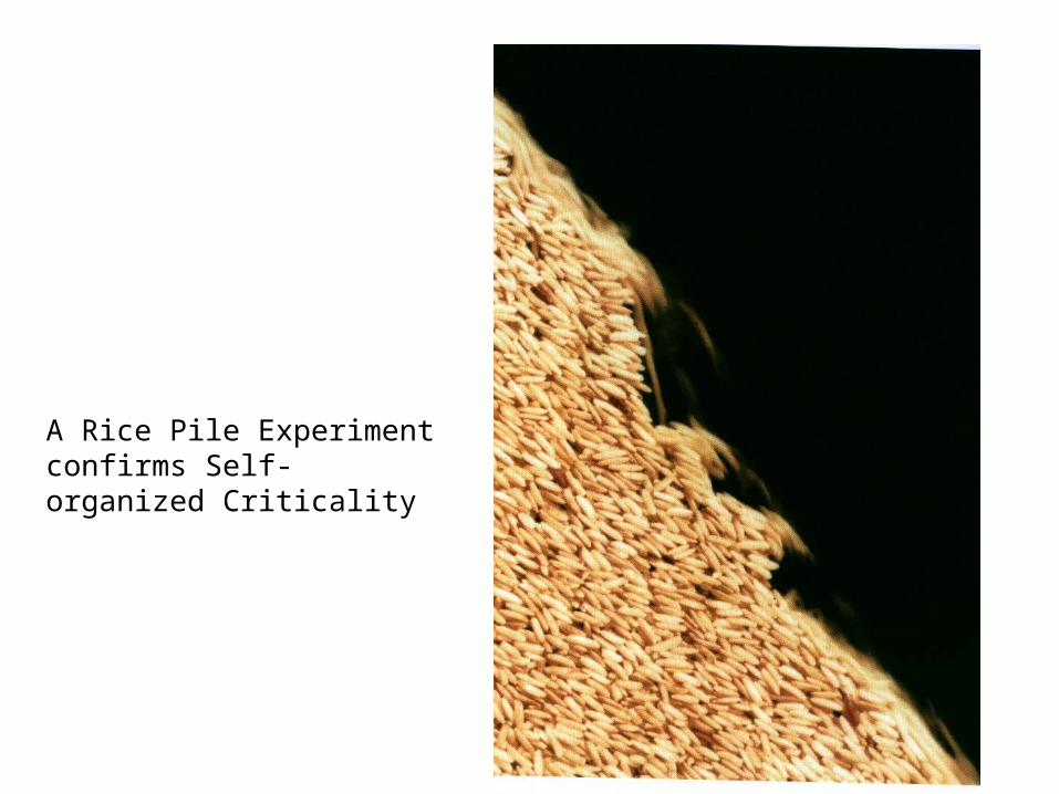
A Rice Pile Experiment confirms Self-organized Criticality

Sand Pile Model

The model is not a realistic model of sand pile. But it captures the basic features of avalanches, and it provides a good illustration of self-organized criticality.

A variable (local height difference) z is defined at each cell •Addition of sand: pick a random cell, increase z by one. z --> z + 1 •Toppling: if z > 4, then z-> z - 4 and  z -> z + 1 for all its neighbors.

Sand Pile Model

Office version of the model (Suggested by Peter Grassberger

Butterfly EffectA small perturbation can have drastic consequences. Chaos

scientists call this the butterfly effect:  A butterfly moving its wings in South American will affect the weather in the United States.

What is the “butterfly effect” in SOC systems such as a sand pile?

In a pile of sand, the majority of perturbations have little effect (leading to no or small avalanches). But there are perturbations that cause big avalanches. But it is difficult to predict which are "more important" sand grains.

A possible example of butterfly effect:     Butterfly ballot at Miami Dade County US presidential election

Second Gulf War

The effect of any perturbation will affect the entire system if we wait long enough.  In a lifetime, everybody will have his 15 minutes of fame (Andy Warhol).   Comparison of two simulations of the earthquake model (starting from small differences in the stress distribution) [applet]

Other Possible Examples of SOC --- Forest Fires

Source: Bruce D. Malamud, Gleb Morein, Donald L. Turcotte, Science, Vol 281, page 1840 (1998).

how to manage

forest?

The World Wide Web

The probability distribution of web sites vs. the number of visitors (in a given day) is a power law(source:Lada A. Adamic)

 

Human Society

Wars and conflicts, migration, city distribution

      Zipf's law describes the relationship between the size of the city and its rank (Rank-Size distribution)         References on Zipf's law       Zipf's law is  named after the Harvard linguistic professor George Kingsley Zipf (1902-1950).

        S  ~  c / R , = 1 in the original Zipf's law 

Zipf law also describes income distribution.

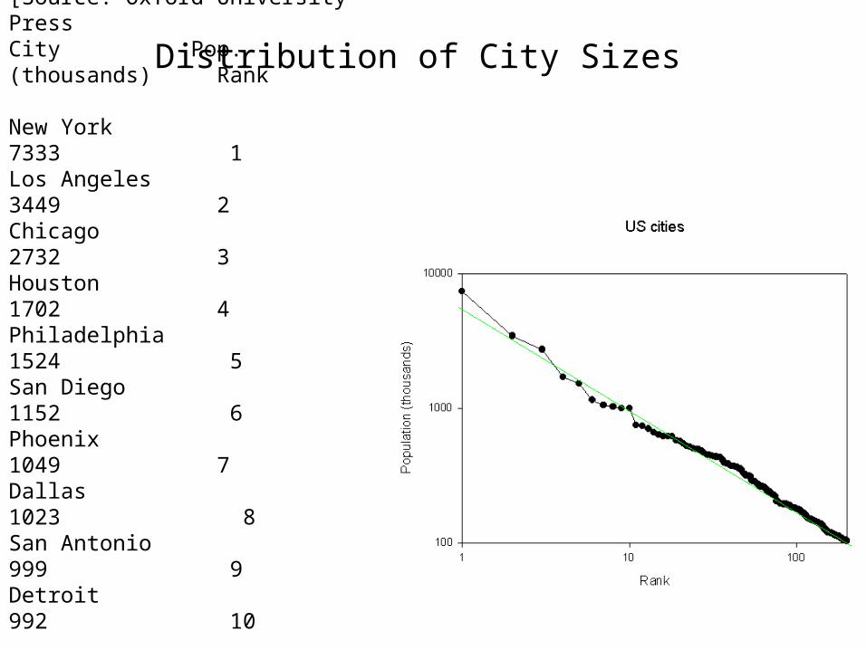
Distribution of City Sizes Data for US cities (~ 0.8) [Source: Oxford University Press City          Pop. (thousands)     Rank

New York             7333             1Los Angeles           3449            2Chicago                 2732            3Houston                 1702            4Philadelphia           1524             5San Diego              1152             6Phoenix                  1049            7Dallas                   1023              8San Antonio           999              9Detroit                 992              10

Distribution of City SizesHow about Chinese cities? ( ~ 0.5)

Cities            Pop. (thousands)     Rank

    Shanghai        8206                 1    BEIJING      7362                  2    Hong Kong      6190                  3    Tianjin           5804                  4    Qingdo           5125                  5    Shenyang       4655                  6    Guangzhou      3918                  7    Wuhan            3833                 8    Tai'an            3825                  9     Harbin           3597                 10

Why is the Zipf exponent for the size distribution of the Chinese cities different from that of the US cities?

What social-economic dynamics gives rise to the difference?

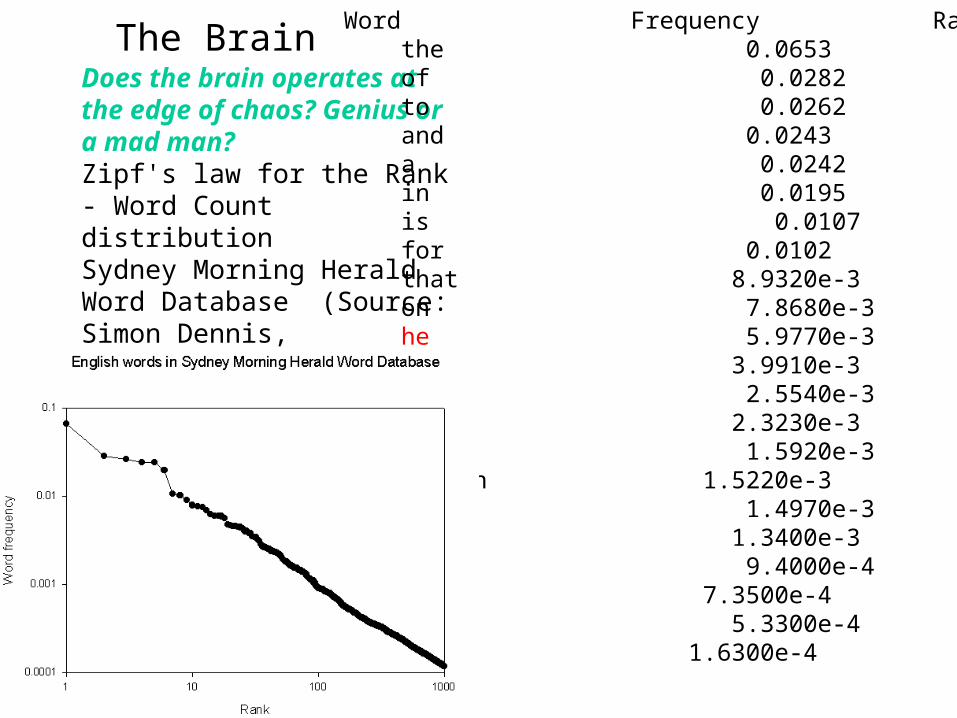
The Brain

Does the brain operates at the edge of chaos? Genius or a mad man?Zipf's law for the Rank - Word Count distributionSydney Morning Herald Word Database  (Source: Simon Dennis, University of Queensland)

Word                Frequency            Rank        the                     0.0653                 1        of                       0.0282                 2        to                       0.0262                 3        and                     0.0243                 4        a                        0.0242                 5        in                       0.0195                  6        is                        0.0107                 7        for                     0.0102                 8        that                   8.9320e-3             9        on                      7.8680e-3            10        he                      5.9770e-3            16        not                    3.9910e-3             26        or                      2.5540e-3            39        you                    2.3230e-3            45        she                     1.5920e-3            63    australian               1.5220e-3            68        her                     1.4970e-3            69    million                    1.3400e-3            78        him                     9.4000e-4            98    market                   7.3500e-4            130      think                    5.3300e-4            171    computer                1.6300e-4            693

Economy and Financial Market

Boom and bust Can one manage the economy by manipulating a

few global parameters? Can the economy be described using equilibrium theory used by many main-stream economists

      Probability of Stock Price Change over an interval,

P(S)  = c /S4

Biological extinction and punctuated equilibrium --- a controversial subject     It is estimated that among four billion species which have existed on the Earth since life first appeared less than 50 million (about 1 percent) are still alive.

Punctuated Equilibrium and Evolution

The pattern of extinction events from the fossil history, as recorded by J. J. Sepkoski.

Extinction events recorded over 600 million years. The curve shows the estimated percentage of species that became extinct during consecutive periods of 5 million years.

Punctuated Equilibrium

From the pattern of extinction events, one can see that

There are periods of relatively little activity (stasis) interrupted by narrow intervals, or bursts, with large activity in the history of biological evolution.

This "punctuated equilibrium" was first noted by Gould and Eldredge. The biological system only appears to be in equilibrium within a certain time scale.

From the data collected by Sepkoski, it is also found that the size distribution of extinction events can roughly be interpreted as a power law, just like the Gutenberg-Richter law for earthquakes.

Does biological system also operate in a critical state?

Evolution in a test tube

Lenski's experiment on E-coli

Evolution in a test tube (Lenski's experiment on E-coli)

Fossil Evidence (Jackson and Cheetham) on Punctuated Equilibrium    Gradualism vs. Punctuated Equilbirum

Bak-Sneppen ModelIt is a very simple toy model of an

ecology of evolving species.

The underlying picture is the one where species interact with each other. The random mutation and then selection of the fitter variants affect the fitness of other species in the global ecology.

  In the Bak-Sneppen model, species are

placed on a one-dimensional ring, for simplicity and bookkeeping. This can be thought of as a food chain (a food web is more realistic).

Initially, the species are assigned random numbers, {fi}, between 0 and 1, where fi represents the fitness of species i.

Each species only interacts with its nearest neighbors. 

f1 f2f3

f4

f5

Scale Free Network• A scale-free network is a specific kind of network

in which the distribution of connectivity is extremely uneven (it follows a power law)

• This kind of connectedness dramatically influences the way the network operates, including how it responds to catastrophic events. The Internet, WWW, many other large-scale networks have been shown to be scale-free networks.

• Physicists Barabasi and Albert constructed a simple model of growing network, which is shown to be scale-free. – Start with a node– A new node is connected to one of the existing nodes.

But the probability of choosing the existing node to connect to

Prob ~ The number of connections it already has– The more connections a node has, the more likely it will

get connected, because the number of agents a node has is equal to how many nodes it connects to.

Dynamics of Networks

• Kauffman’s NK Boolean network– Random network– Each node has K inputs.

s(t) = f({si(t-1)}, i=1,..,K)

– K = 1 fixed point– K = 2 periodic (the distribution of the periods,

P(T), is a power law)– K > 3 chaotic

In real biological network, K is typically much greater than 3; but the network is stable

Dynamics of Networks• Growing Directed Network

– Network is grown by adding nodes one by one (starting with an initial cluster)

– Each node has K inputs. s(t) = f({si(t-1)}, i=1,..,K)

But the new node cannot influence the existing nodes (like a citation network)

– Stable for all K (the maximum period is 2K+1)– Dynamics insensitive to preferential attachment. Size

distribution of descendant clusters is a power law.• Growing Directed Network with a fraction of link reversals

– Appears to be critical (the distribution of the periods is a power law)

Could the growing directed network with a fraction of link reversals serves as a better model for biological networks?

Conclusions

• Power-law statistics often means the underlying dynamics is critical. Examples: Earthquakes, forest fires.

• Such critical states emerge naturally without fine tuning Self-organized Criticality

• Criticality Universality. It is possible to understand universal properties using simple models

• Many interesting networks also exhibit power law statistics.

• Network organization and dynamics are closely related. • Emergence of power laws in network dynamics