overview of neural network architectures for graph ...pv273/slides/uclgraph.pdf · overview of...

Overview of neural network architecturesfor graph-structured data analysisPetar Velickovic

Artificial Intelligence GroupDepartment of Computer Science and Technology, University of Cambridge, UK

UCL AI Journal Club 19 February 2018

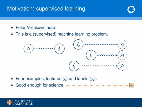
Motivation: supervised learning

I Petar Velickovic here!I This is a (supervised) machine learning problem.

~f1~f2

~f3

~f4

y1

y2

y3

y4

I Four examples, features (~fi ) and labels (yi ).I Good enough for science.······················································X

tst Gentlemen, I give you graphs. The inputs of tomorrow!



~f1~f2

~f3

~f4

y1

y2

y3

y4

I Four examples, features (~fi ) and labels (yi ).I Good enough for science. Not Aperture Science!···············X

tst Gentlemen, I give you graphs. The inputs of tomorrow!



~f1~f2

~f3

~f4

y1

y2

y3

y4

I Four examples, features (~fi ) and labels (yi ).I Good enough for science. Not Aperture Science!···············XI Gentlemen, I give you graphs. The inputs of tomorrow!

Graphs are everywhere!

Introduction

I In this talk, I will demonstrate some of the popularmethodologies that leverage neural networks for processinggraph-structured inputs.

I Although the earliest approaches to this problem date to thelate 90s, it has caught traction only in the recent five years (witha proper explosion happening throughout 2017)!

I For early references, you may investigate the works of Sperduti& Starita (1997) and Frasconi et al. (1998), IEEE TNNLS.

I There’s at least ten submissions to ICLR 2018 alone thatattempt solving the same graph problems in different ways.

Mathematical formulation

I We will focus on the node classification problem:I Input: a matrix of node features, F ∈ RN×F , with F features in

each of the N nodes, and an adjacency matrix, A ∈ RN×N .I Output: a matrix of node class probabilities, Y ∈ RN×C , such

that Yij = P(Node i ∈ Class j).

I We also assume, for simplicity, that the edges are unweightedand undirected:

I That is, Aij = Aji =

{1 i ↔ j0 otherwise

but many algorithms we will cover are capable of generalisingto weighted and directed edges.

I There are two main kinds of learning tasks in this space. . .

Transductive learning

Training algorithm sees all features (including test nodes)!

Inductive learning

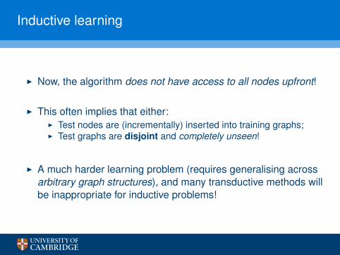
I Now, the algorithm does not have access to all nodes upfront!

I This often implies that either:I Test nodes are (incrementally) inserted into training graphs;I Test graphs are disjoint and completely unseen!

I A much harder learning problem (requires generalising acrossarbitrary graph structures), and many transductive methods willbe inappropriate for inductive problems!

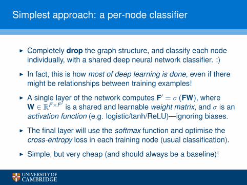
Simplest approach: a per-node classifier

I Completely drop the graph structure, and classify each nodeindividually, with a shared deep neural network classifier. :)

I In fact, this is how most of deep learning is done, even if theremight be relationships between training examples!

I A single layer of the network computes F′ = σ (FW), whereW ∈ RF×F ′

is a shared and learnable weight matrix, and σ is anactivation function (e.g. logistic/tanh/ReLU)—ignoring biases.

I The final layer will use the softmax function and optimise thecross-entropy loss in each training node (usual classification).

I Simple, but very cheap (and should always be a baseline)!

Augmenting the per-node classifier

I Many earlier approaches to incorporating graph structure willretain the per-node shared classifier, but incorporate graphstructure by either:

I constraining its learnt features depending on the graph edges;I augmenting the input layer with structural node features.

I I will now briefly cover both of those approaches.

Injecting structure: semi-supervised embedding

I Introduced by Weston et al. (ICML 2008), generalising the workof Zhu et al. (ICML 2003) and Belkin et al. (JMLR 2006) toneural networks.

~fi

~fj

?

yi

yj

I Under the assumption that the edges encode node similarity,further constrain the learnt representations of nodes to beclose/distant depending on presence of edge!

Semi-supervised embedding loss

I Essentially, the loss function to optimise is augmented with a(dis)similarity constraint, Lsim:

L = L0 + λLsim

where L0 is the usual supervised learning loss (e.g.cross-entropy), and λ is a hyperparameter.

I One way to define Lsim:

Lsim =∑

i

∑j∈Ni

‖~hi − ~hj‖2 +∑j /∈Ni

max(

0,m − ‖~hi − ~hj‖2)

where Ni is the neighbourhood of node i , ~hi is (one of) itshidden layer’s outputs, and m is a hyperparameter.

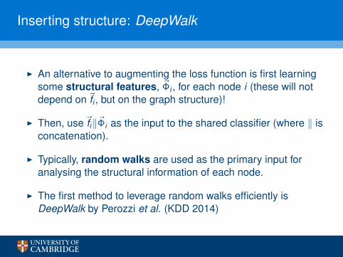
Inserting structure: DeepWalk

I An alternative to augmenting the loss function is first learningsome structural features, ~Φi , for each node i (these will notdepend on ~fi , but on the graph structure)!

I Then, use ~fi‖~Φi as the input to the shared classifier (where ‖ isconcatenation).

I Typically, random walks are used as the primary input foranalysing the structural information of each node.

I The first method to leverage random walks efficiently isDeepWalk by Perozzi et al. (KDD 2014)

Overview of DeepWalk

I Start by random features ~Φi for each node i .

I Sample a random walkWi , starting from node i .

I For node x at step j , x =Wi [j], and a node y at stepk ∈ [j − w , j + w ], y =Wi [k ], modify ~Φx to maximiselogP(y |~Φx ) (obtained from a neural network classifier).

I Inspired by skip-gram models in natural language processing:to obtain a good vector representation of a word, its vectorshould allow us to easily predict the words that surround it.

Overview of DeepWalk, cont’d

I Expressing the full P(y |~Φx ) distribution directly, even for asingle layer neural network, where

P(y |~Φx ) = softmax(~wTy~Φx ) =

exp(~wT

y~Φx

)∑

z exp(~wT

z~Φx

)is prohibitive for large graphs, as we need to normalise acrossthe entire space of nodes—making most updates vanish.

I To rectify, DeepWalk expresses it as a hierarchical softmax—atree of binary classifiers, each halving the node space.

DeepWalk in action

Later improved by LINE (Tang et al., WWW 2015) and node2vec(Grover & Leskovec, KDD 2016), but main idea stays the same.

Incorporating labels and features: Planetoid

I Methods such as DeepWalk are still favourable when dealingwith fully unsupervised graph problems, as they don’t dependon having any labels or features in the nodes!

I However, if we have labels/features, why not use them?

I The essence behind Planetoid (Predicting Labels AndNeighbours with Embeddings Transductively Or Inductivelyfrom Data), by Yang et al. (ICML 2016).

Planetoid’s sampling strategy: Negative sampling

I Addresses the issue with P(y |~Φx ) by employing negativesampling; predict instead P(γ|~Φx , ~wy ), where γ ∈ {0,1}.

I Essentially, use a binary classifier:

P(γ|~Φx , ~wy ) = σ(~wT

y~Φx

)where σ is the logistic sigmoid function. Now each update willfocus only on one node’s weight vector rather than all of them!

I γ = 1 implies that nodes x and y are a “positive” pair (moredetail in the next slide).

Planetoid’s sampling strategy: Sampling pairs

I Planetoid retains DeepWalk’s idea of predicting proximal nodesin random walks.

I Sample two nodes a and b that are close enough in a randomwalk, optimise the classifier to predict γ = 1.

I Sample two nodes a and b uniformly at random, optimise theclassifier to predict γ = 0.

I It also injects label information:I Sample two nodes a and b with same labels (ya = yb), optimise

the classifier to predict γ = 1.I Sample two nodes a and b with different labels (ya 6= yb),

optimise the classifier to predict γ = 0.

Planetoid in action

C1 C1

? ?

C2 ?

1

2 3

4

5 6

Consider this example graph, with three labelled nodes.I will now illustrate the two phases of Planetoid.

Planetoid in action: Random walk-based sampling

C1 C1

? ?

C2 ?

1

2 3

4

5 6

Sample from a random walk—can take e.g. nodes 1 and 4 withγ = 1, and nodes 1 and 5 with γ = 0.

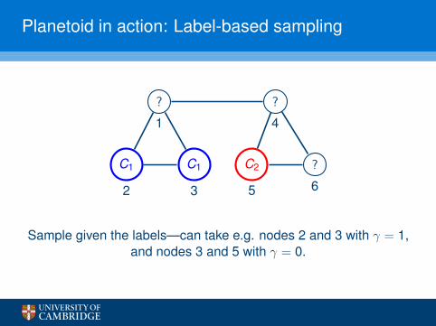
Planetoid in action: Label-based sampling

C1 C1

? ?

C2 ?

1

2 3

4

5 6

Sample given the labels—can take e.g. nodes 2 and 3 with γ = 1,and nodes 3 and 5 with γ = 0.

Planetoid’s inductive dataflow

I In an inductive setting, the structural features ~Φi can no longerbe independently learned—need to adapt to unseen nodes!

I The inductive version of Planetoid forces ~Φi to directly dependon ~fi—you guessed it—by employing a neural network. :)

~fi

~Φi

‖ yi

γ(i , j)

NN1

NN2

×~wj

Explicit graph neural network methodologies

I All methods covered so far have used a shared classifier thatclassifies each node independently, with graph structureinjected only indirectly.

I We will from now restrict our attention solely to methods thatdirectly leverage the graph structure when computingintermediate features.

I Main idea: Compute node representations ~hi based on theinitial features ~fi and the graph structure, and then use ~hi toclassify each node independently (as before).

Graph Neural Networks

I The first prominent example of such an architecture are GraphNeural Networks (GNNs) presented first in Gori et al. (IJCNN2005) and then in Scarselli et al. (TNNLS 2009).

I Start with randomly initialised ~h(0)i , then at each timestep

propagate as follows (slightly different than original paper,assuming only undirected edges of one type):

~h(t)i =

∑j∈Ni

f(~h(t−1)

j

)where f is a propagation model, expressed as a usual neuralnetwork linear layer:

f (~hi) = W~hi + ~b

where W and ~b are learnable weights and biases, respectively.

Graph Neural Networks, cont’d

I As backpropagating through time is expensive, the authors ofGNNs further constrain f to be a contractive map. This impliesthat the ~hi vectors will always converge to a unique fixed point!

I Iterate until convergence (for T steps), then classify using ~h(T )i .

Train using the Almeida-Pineda extension of backpropagation(Almeida, 1990; Pineda, 1987).

I Arguably, too restrictive. Also, impossible to injectproblem-specific information into ~h(0)

i (as will always convergeto same value regardless of initialisation).

Gated Graph Neural Networks

I An extension to GNNs, known as Gated Graph NeuralNetworks (GGNNs) by Li et al. (ICLR 2016), brought thebleeding-edge deep learning practices to GNNs.

I Propagate for a fixed number of steps, and do not restrict thepropagation model to be contractive.

I This enables conventional backpropagation.I It also allows us to meaningfully initialise the model!

I Leverage a more sophisticated propagation model (employingtechniques such as gating) to surpass GNN performance.

GGNN propagation rule

I Initialise as ~h(0)i = ~fi‖~0 (append zeroes for extra capacity).

I Then propagate as follows (slightly different than original paper,assuming only undirected edges of one type):

~a(t)i = bi +

∑j∈Ni

~h(t−1)

~h(t)i = tanh

(W~a(t)

i

)I Now, extend this to incorporate gating mechanisms, to prevent

full overwrite of ~h(t−1)i by ~h(t)

i .I Basically, learn (from ~a(t)

i and ~h(t−1)i ) how much to overwrite.

Full GGNN propagation rule

I The full propagation model is as follows:

~a(t)i = bi +

∑j∈Ni

~h(t−1)j

~r (t)i = σ(

Wr~a(t)i + Ur~h(t−1)

i

)~z(t)

i = σ(

Wz~a(t)i + Uz~h(t−1)

i

)~h(t)

i = tanh(

W~a(t)i + U

(~r (t)i � ~h

(t−1)i

))~h(t)

i = (1− ~z(t)i )� ~h(t−1)

i + ~z(t)i �

~h(t)i

where � is elementwise vector multiplication, ~ri and ~zi are resetand update gates, and σ is the logistic sigmoid function.

The silver bullet—a convolutional layer

I GGNNs feature a “time-step” operation which should be veryfamiliar to those of you who have already worked with recurrentneural networks (such as LSTMs).

I These are designed for data that changes sequentially;however, our graphs have static features!

I It would be more appropriate if we could somehow generalisethe convolutional operator (as used in CNNs) to operate onarbitrary graphs!

I An excellent “common framework” for many of the approachesto be listed now has been presented in “Neural MessagePassing for Quantum Chemistry”, by Gilmer et al. (ICML 2017).

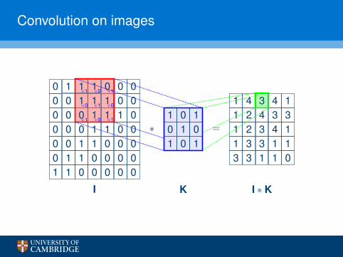
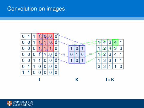
Convolution on images

0 1 1 1 0 0 00 0 1 1 1 0 00 0 0 1 1 1 00 0 0 1 1 0 00 0 1 1 0 0 00 1 1 0 0 0 01 1 0 0 0 0 0

I

∗1 0 10 1 01 0 1

K

=

1 4 3 4 11 2 4 3 31 2 3 4 11 3 3 1 13 3 1 1 0

I ∗ K

1 0 10 1 01 0 1

×1 ×0 ×1

×0 ×1 ×0

×1 ×0 ×1

Challenges with graph convolutions

I Desirable properties for a graph convolutional layer:I Computational and storage efficiency (∼ O(V + E));I Fixed number of parameters (independent of input size);I Localisation (acts on a local neighbourhood of a node);I Specifying different importances to different neighbours;I Applicability to inductive problems.

I Fortunately, images have a highly rigid and regular connectivitypattern (each pixel “connected” to its eight neighbouringpixels), making such an operator trivial to deploy (as a smallkernel matrix which is slided across).

I Arbitrary graphs are a much harder challenge!

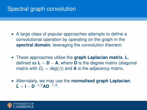
Spectral graph convolution

I A large class of popular approaches attempts to define aconvolutional operation by operating on the graph in thespectral domain, leveraging the convolution theorem.

I These approaches utilise the graph Laplacian matrix, L,defined as L = D− A, where D is the degree matrix (diagonalmatrix with Dii = deg(i)) and A is the adjacency matrix.

I Alternately, we may use the normalised graph Laplacian,L = I− D−1/2AD−1/2.

Graph Laplacian example

1 2 3

4

5

6 L =

2 −1 0 0 −1 0−1 3 −1 0 −1 00 −1 2 −1 0 00 0 −1 3 −1 −1−1 −1 0 −1 3 00 0 0 −1 0 1

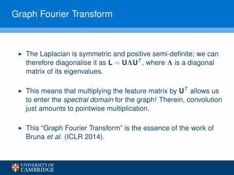
Graph Fourier Transform

I The Laplacian is symmetric and positive semi-definite; we cantherefore diagonalise it as L = UΛUT , where Λ is a diagonalmatrix of its eigenvalues.

I This means that multiplying the feature matrix by UT allows usto enter the spectral domain for the graph! Therein, convolutionjust amounts to pointwise multiplication.

I This “Graph Fourier Transform” is the essence of the work ofBruna et al. (ICLR 2014).

Graph Fourier Transform, cont’d

I To convolve two signals using the convolution theorem:

conv(~x , ~y) = U(

UT~x � UT~y)

I Therefore, a learnable convolutional layer amounts to:

~h′i = U(~w � UT W~hi

)where ~w is a learnable vector of weights, and W ∈ RF ′×F is ashared, learnable, feature transformation.

I Downsides:I Computing U is O(V 3)—infeasible for large graphs!I One independent weight per node—not fixed!I Not localised!

Chebyshev networks

I These issues have been overcome by ChebyNets, the work ofDefferrard et al. (NIPS 2016).

I Rather than computing the Fourier transform, use the relatedfamily of Chebyshev polynomials of order k , Tk :

~h′i =K∑

k=0

wkTk (L)W~hi

I These polynomials have a recursive definition, highlysimplifying the computation:

T0(x) = 1 T1(x) = x Tk (x) = 2xTk−1(x)− Tk−2(x)

Properties of Chebyshev networks

I Owing to its recursive definition, we can compute the outputiteratively as

∑Kk=0 wk~tk , where:

~t0 = W~hi ~t1 = LW~hi ~tk = 2L~tk−1 −~tk−2

where each step constitutes a sparse multiplication with L.

I The number of parameters is fixed (equal to K weights).

I Note that Tk (L) will be a (weighted) sum of all powers of L upto Lk . This means that Tk (L)ij = 0 if dist(i , j) > k !

=⇒ The operator is K-localised!

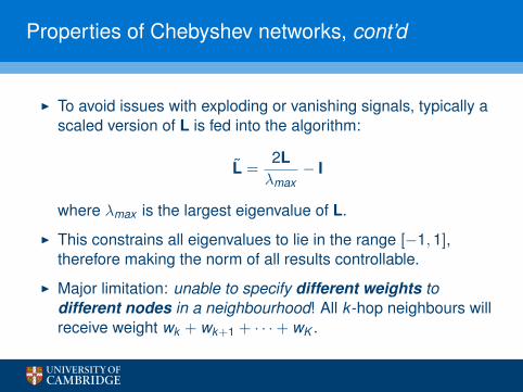
Properties of Chebyshev networks, cont’d

I To avoid issues with exploding or vanishing signals, typically ascaled version of L is fed into the algorithm:

L =2Lλmax

− I

where λmax is the largest eigenvalue of L.

I This constrains all eigenvalues to lie in the range [−1,1],therefore making the norm of all results controllable.

I Major limitation: unable to specify different weights todifferent nodes in a neighbourhood! All k -hop neighbours willreceive weight wk + wk+1 + · · ·+ wK .

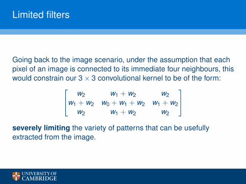
Limited filters

Going back to the image scenario, under the assumption that eachpixel of an image is connected to its immediate four neighbours, thiswould constrain our 3× 3 convolutional kernel to be of the form: w2 w1 + w2 w2

w1 + w2 w0 + w1 + w2 w1 + w2w2 w1 + w2 w2

severely limiting the variety of patterns that can be usefullyextracted from the image.

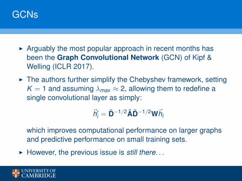
GCNs

I Arguably the most popular approach in recent months hasbeen the Graph Convolutional Network (GCN) of Kipf &Welling (ICLR 2017).

I The authors further simplify the Chebyshev framework, settingK = 1 and assuming λmax ≈ 2, allowing them to redefine asingle convolutional layer as simply:

~h′i = D−1/2AD−1/2W~hi

which improves computational performance on larger graphsand predictive performance on small training sets.

I However, the previous issue is still there. . .

Applicability to inductive problems

I Another fundamental constraint of all spectral-based methodsis that the learnt filter weights are assuming a particular, fixed,graph Laplacian.

I This makes them theoretically inadequate for arbitraryinductive problems!

I We have to move on to non-spectral approaches. . .

Molecular fingerprinting networks

I An early notable approach towards such methods is the workof Duvenaud et al. (NIPS 2015).

I Here, the method adapts to processing with various degrees bylearning a separate weight matrix Hd for each node degree d .

I The authors dealt with an extremely specific domain problem(molecular fingerprinting), where node degrees could neverexceed five; this does not scale to graphs with very widedegree distributions.

GraphSAGE

I Conversely, the recently-published GraphSAGE model byHamilton et al. (NIPS 2017) aims to restrict every degree tobe the same (by sampling a fixed-size set of neighbours ofevery node, during both training and inference).

I Inherently drops relevant data—limiting the set of neighboursvisible to the algorithm.

I Impressive performance was achieved across a variety ofinductive graph problems. However, the best results were oftenachieved with an LSTM-based aggregator, which is unlikely tobe optimal.

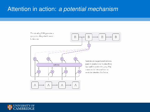
Attentional mechanisms

I One of the latest non-spectral techniques leverages anattentional mechanism (originally published by Bahdanau et al.(ICLR 2015)), which is now a de facto standard for sequentialprocessing tasks.

I Computes linear combinations of the input features to generatethe output. The coefficients of these linear combinations areparametrised by a shared neural network!

I Intuitively, allows each component of the output to generate itsown combination of the inputs—thus, different outputs paydifferent levels of attention to the respective inputs.

Attention in action: a potential mechanism

Attention in action: machine translation

Self-attention

I A rather exciting development in this direction concernsself-attention; a scenario where the input attends over itself:

αij = a(~hi , ~hj)

~h′i =∑

j

softmaxj(αij)~hj

where a(~x , ~y) is a neural network (the attention mechanism).

I Critically, this is parallelisable across all input positions!

I Vaswani et al. (NIPS 2017) have successfully demonstratedthat this operation is self-sufficient for achieving state-of-the-arton machine translation.

Graph Attention Networks

I My recent ICLR 2018 publication—in collaboration with theMontreal Institute for Learning Algorithms (MILA)—proposingGraph Attention Networks (GATs), leverages exactly theself-attention operator!

I In its naıve form, the operator would compute attentioncoefficients over all pairs of nodes.

I To inject the graph structure into the model, we restrict themodel to only attend over a node’s neighbourhood whencomputing its coefficient!

GAT equations

I To recap, a single attention head of a GAT model performs thefollowing computation:

eij = a(W~hi ,W~hj)

αij =exp(eij)∑

k∈Niexp(eik )

~h′i = σ

∑j∈Ni

αijW~hj

I Some further optimisations (like multi-head attention and

dropout on the αij values) help further stabilise and regularisethe model.

A single GAT step, visualised

αij

~a

softm

axj

W~hi W~hj

~h1

~h2

~h3

~h4

~h5

~h6

~α16

~α11

~α12

~α13

~α 14

~α15

~h′1concat/avg

GAT analysis

I Computationally efficient: attention computation can beparallelised across all edges of the graph, and aggregationacross all nodes!

I Storage efficient—a sparse version does not require storingmore than O(V + E) entries anywhere;

I Fixed number of parameters (dependent only on the desirablefeature count, not on the node count);

I Trivially localised (as we aggregate only overneighbourhoods);

I Allows for (implicitly) specifying different importances todifferent neighbours.

I Readily applicable to inductive problems (as it is a sharededge-wise mechanism)!

GAT performance

I It seems that we have finally satisfied all of the majorrequirements for our convolution!

I How well does it perform?

Datasets under study

Table: Summary of the datasets used in our experiments.

Transductive InductiveCora Citeseer Pubmed PPI

# Nodes 2708 3327 19717 56944 (24 graphs)# Edges 5429 4732 44338 818716# Features/Node 1433 3703 500 50# Classes 7 6 3 121 (multilabel)# Training Nodes 140 120 60 44906 (20 graphs)# Validation Nodes 500 500 500 6514 (2 graphs)# Test Nodes 1000 1000 1000 5524 (2 graphs)

Results on Cora/Citeseer/Pubmed

Transductive

Method Cora Citeseer Pubmed

MLP 55.1% 46.5% 71.4%ManiReg 59.5% 60.1% 70.7%SemiEmb 59.0% 59.6% 71.7%LP 68.0% 45.3% 63.0%DeepWalk 67.2% 43.2% 65.3%ICA 75.1% 69.1% 73.9%Planetoid 75.7% 64.7% 77.2%Chebyshev 81.2% 69.8% 74.4%GCN 81.5% 70.3% 79.0%MoNet 81.7 ± 0.5% — 78.8 ± 0.3%

GCN-64∗ 81.4 ± 0.5% 70.9 ± 0.5% 79.0 ± 0.3%GAT (ours) 83.0 ± 0.7% 72.5 ± 0.7% 79.0 ± 0.3%

Results on PPI

Inductive

Method PPI

Random 0.396MLP 0.422GraphSAGE-GCN 0.500GraphSAGE-mean 0.598GraphSAGE-LSTM 0.612GraphSAGE-pool 0.600

GraphSAGE∗ 0.768Const-GAT (ours) 0.934 ± 0.006GAT (ours) 0.973 ± 0.002

Here, Const-GAT is a GCN-like inductive model.

Applications

I I will conclude with an overview of a few interesting applicationsof GCN- and GAT-like models.

I This list is by no means exhaustive, and represents only what Ihave been able to find thus far. :)

Citation networks

Velickovic et al. (ICLR 2018)

Molecular fingerprinting

Duvenaud et al. (NIPS 2015)

Molecular fingerprinting, cont’d

Duvenaud et al. (NIPS 2015)

Learning on manifolds

The MoNet framework, by Monti et al. (CVPR 2017)

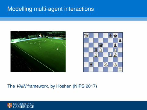
Modelling multi-agent interactions

The VAIN framework, by Hoshen (NIPS 2017)

Cortical mesh segmentation

Cucurull et al. (NIPS BigNeuro 2017)Currently preparing an extended version to submit to MICCAI. . .

Thank you!

[email protected]

http://www.cst.cam.ac.uk/∼pv273/

https://github.com/PetarV-/GAT

overview of neural network architectures for graph ...pv273/slides/uclgraph.pdf · overview of...

Documents