Overview of OptionsFIN 562 – Summer 2006

July 5, 2006

Why are options important?

• Options are common risk management instruments.

• Compensation plans have made extensive use of options.

• Implications for corporate investment – “real” options.

• Options are sometimes embedded in debt contracts – “convertible” debt.

Basic option terminology

• Call option: “Right to buy.”• Put option: “Right to sell.”• European option: Exercise decision is

made only at option’s maturity date.• American option: Can be exercised

prior to maturity date.• Exercise price: Also known as “strike

price” – this is the price at which option can be exercised.

• Premium: Option’s price

Option payoffs

• Call option• Strike price of $25

25

25

payoff

Price of underlying50

Option payoffs (p. 2)

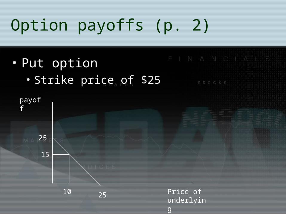
• Put option• Strike price of $25

25

25

payoff

Price of underlying

10

15

More option terminology

• In the money• Call option (on stock): stock price > exercise price

(S > X)• Put option: stock price < exercise price (S < X)

• Out of the money• Call option: S < X• Put option: S > X

• At the money• S = X

• Intrinsic Value• Call option: Max (S – X, 0)• Put option: Max (X – S, 0)

Payoffs to selling (writing) options

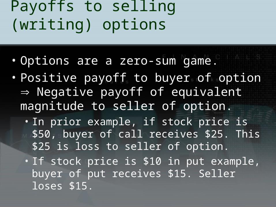
• Options are a zero-sum game.• Positive payoff to buyer of option

Negative payoff of equivalent magnitude to seller of option.• In prior example, if stock price is $50,

buyer of call receives $25. This $25 is loss to seller of option.

• If stock price is $10 in put example, buyer of put receives $15. Seller loses $15.

Why sell options?

• Seller collects a premium from the buyer.

• Can think of this like a payment for insurance.

• Seller and buyer must agree on a price that is “fair.”

• We’ll get to basics of option valuation later!

Put-call parity

• Law of One Price: price paid for two identical assets must be equivalent.

• Here are two investment strategies:• Buy call option with exercise price, X, AND

buy a risk-free bond (with same maturity as call) for present value of X.

• Buy put option with exercise price, X, AND buy a share of the underlying stock.

• Payoffs from the 2 strategies are equal.

Put-call parity (cont’d)

• Put-call parity for European options:• Value of call + Xe-rT = Value of put + Share price• Suppose Microsoft Jan 2007 25 call is available for

$1.35. Current Microsoft price is $24. Risk-free rate is 5%. What should the value of a MSFT Jan 2007 25 put?

• Value of put = 1.35 + 25*0.9672 – 24 = $1.53• From this example, you can see that buying a put

option is very much like selling a share of stock AND buying a call. Can you draw the payoff diagrams to see why these are similar strategies?

What determines option values?

• Price of the underlying.• Holding exercise price constant, call’s

value increases with price, while put’s value decreases.

• Volatility of the underlying’s price.• More volatility increases option value.

• Time until expiration of the option.• More time until expiration increase option

value.• Interest rates.

Valuing the option: 1-period binomial model

• Assume “simple” world: stock price = $100, risk-free rate = 6%.• State 1 (in 1 period): price = 120• State 2: price = 90• What is value of call with X = $100?• Let p = (0.06 – (-0.10)) / (0.20 – (-0.10)) =

0.5333….• Then, expected payoff = 0.5333($20) +

0.4667($0) = $10.6666….• Value = $10.6666 / (1.06) = $10.06

Binomial model: 1-period example (cont’d)

• Suppose you buy 2/3 share of the underlying at $100 and sell 1 call option for $10.06.• If stock price goes up to $120:

• Profit on sale of 2/3 share of stock = $13.33• Loss on option = ($20)• Add option premium of $10.06• Total = 13.33 + 10.06 – 20 = $3.39• Initial investment = $66.67 – 10.06 = 56.61• ROI = 3.39 / 56.61 = 6%

• If stock price goes down to $90:• Profit on sale of stock = ($6.67), gain on option = 10.06,

total = 10.06 – 6.67 = 3.39, ROI = 6%

Risk-free valuation

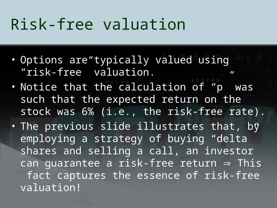
• Options are typically valued using “risk-free” valuation.

• Notice that the calculation of “p” was such that the expected return on the stock was 6% (i.e., the risk-free rate).

• The previous slide illustrates that, by employing a strategy of buying “delta” shares and selling a call, an investor can guarantee a risk-free return This fact captures the essence of risk-free valuation!

Binomial model: 2-periods and beyond

• We can “break” the binomial model into as many periods as we deem appropriate.

• The option value is determined by starting at the “ends” of the binomial tree and working backward.

• We continue to employ a risk-neutral valuation methodology.

Example: 2-period binomial model

• Stock is at $100 and can either move up 10% or down 5% each period. Risk-free rate is 3% per period.

110

95

121

104.5

90.25

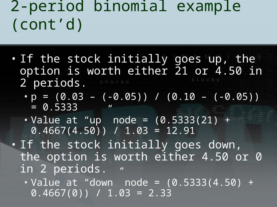
2-period binomial example (cont’d)

• If the stock initially goes up, the option is worth either 21 or 4.50 in 2 periods.• p = (0.03 – (-0.05)) / (0.10 – (-0.05)) =

0.5333• Value at “up” node = (0.5333(21) +

0.4667(4.50)) / 1.03 = 12.91• If the stock initially goes down, the

option is worth either 4.50 or 0 in 2 periods.• Value at “down” node = (0.5333(4.50) +

0.4667(0)) / 1.03 = 2.33

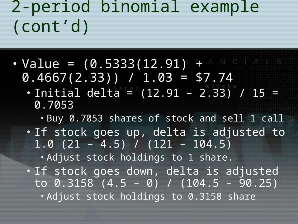
2-period binomial example (cont’d)

• Value = (0.5333(12.91) + 0.4667(2.33)) / 1.03 = $7.74• Initial delta = (12.91 – 2.33) / 15 = 0.7053

• Buy 0.7053 shares of stock and sell 1 call

• If stock goes up, delta is adjusted to 1.0 (21 – 4.5) / (121 – 104.5)• Adjust stock holdings to 1 share.

• If stock goes down, delta is adjusted to 0.3158 (4.5 – 0) / (104.5 – 90.25)• Adjust stock holdings to 0.3158 share

2-period binomial example (investments)

• Initial investment:• Stock = $70.53• Sell option @ $7.74 total investment = $62.79

• If stock goes up:• Buy another 0.2947 shares of stock at $110

($32.417). Total investment = $95.21 (62.79 + 32.42)

• If stock goes down:• Sell 0.3895 shares of stock at $95 ($37). Total

investment = $25.79 (62.79 – 37)

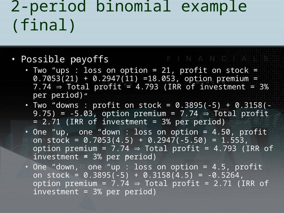
2-period binomial example (final)

• Possible payoffs• Two “ups”: loss on option = 21, profit on stock =

0.7053(21) + 0.2947(11) =18.053, option premium = 7.74 Total profit = 4.793 (IRR of investment = 3% per period)

• Two “downs”: profit on stock = 0.3895(-5) + 0.3158(-9.75) = -5.03, option premium = 7.74 Total profit = 2.71 (IRR of investment = 3% per period)

• One “up,” one “down”: loss on option = 4.50, profit on stock = 0.7053(4.5) + 0.2947(-5.50) = 1.553, option premium = 7.74 Total profit = 4.793 (IRR of investment = 3% per period)

• One “down,” one “up”: loss on option = 4.5, profit on stock = 0.3895(-5) + 0.3158(4.5) = -0.5264, option premium = 7.74 Total profit = 2.71 (IRR of investment = 3% per period)

Black-Scholes model: Introduction

• The binomial model assumes stock prices follow “discrete” path.

• Suppose prices follow “continuous” path

• A “closed form” equation can be developed for valuing options• Black-Scholes model

Variables in the Black-Scholes model

• S = Stock price• X = Exercise price• r = risk-free rate• T = years until maturity = annual standard deviation of stock

returns (volatility)• N(d1) = cumulative normal distribution

function evaluated at “d1.” Excel function = normsdist(.)

• N(d2) = cumulative normal distribution function evaluated at “d2.”

Variables in the Black-Scholes model (cont’d)

Tdd 12

T

TrXS

d

)

2()ln(

1

2

)2(**)1(* dNeXdNSC rT

Example of Black-Scholes valuation

• See option value spreadsheet• Base case

• Stock price (S) = $30• Exercise price (X) = $30• Years until maturity = 6• Risk-free rate = 4.5%• Standard deviation = 40%• Dividend yield = 1%• Call value = 12.49 & Put value = 6.81 (derived from put-

call parity)

• Vary stock price & volatility• Introduce “delta” and “vega”

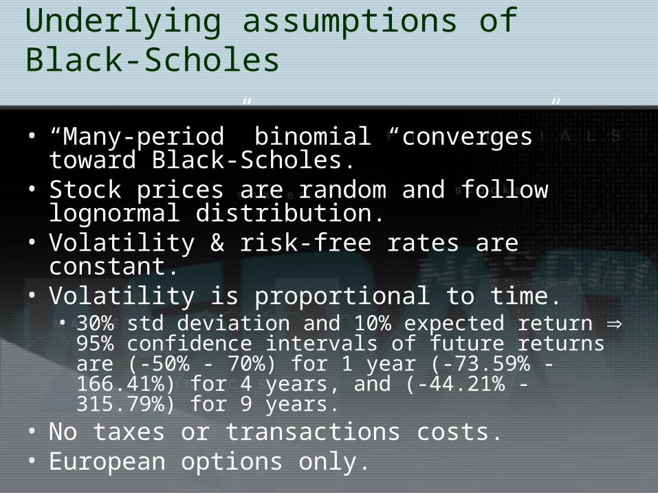
Underlying assumptions of Black-Scholes

• “Many-period” binomial “converges” toward Black-Scholes.

• Stock prices are random and follow lognormal distribution.

• Volatility & risk-free rates are constant.• Volatility is proportional to time.

• 30% std deviation and 10% expected return 95% confidence intervals of future returns are (-50% - 70%) for 1 year (-73.59% - 166.41%) for 4 years, and (-44.21% - 315.79%) for 9 years.

• No taxes or transactions costs.• European options only.

Summary of option valuation techniques

• Binomial: • “easy” if assume one or two periods.• More complexity as we assume “realistically” more discrete

periods use computing power.• With computers, can build flexible models to take possible

complicating factors into account (early exercise, time-varying volatility, risk aversion, vesting considerations, etc.)

• Black-Scholes• Highly restrictive assumptions• Convenient tool for getting “first-pass” assessment of

option value.• Often used in practice because of ease of use.• Calculation of “implied volatility” is possible from the model

and is often used as a better measure of stock’s expected standard deviation (as opposed to historical measure).

Real options

• Capital investment decisions often include embedded options.

• Sole use of NPV criterion might give “false negative” on a project including “real options.”

• Project value with real options embedded = NPV of investment + value of real option

Possible real options acquired with capital investment

• Option to pursue follow-on investments• Does the investment generate capabilities for

future profitable investment?• PC example.• Investment in land with uncertain development

prospects.• Buying currently unprofitable oil & gas reserves.

• Option to abandon• Is there uncertainty regarding when it will be

optimal to “salvage” the investment?• “Shutting in” gold mine

Other real options

• Timing option• Invest now (NPV) vs. wait (option value)• If Option value > NPV, optimal to wait

• Designing flexible production systems• Aircraft purchase options

Challenges of utilizing real options as decision tool

• “Risk-neutral” framework likely cannot yield correct value.• Black-Scholes will always overvalue real options

because unable to design risk-free hedge (like in previous valuation examples).

• Have to use binomial model.• What’s the discount rate?

• Lack of structure to help in designing binomial model.

• If competitors also have same real options, affects value of yours.

Other applied options in corporate finance

• Equity of firm near financial distress• Stockholders own put option (written by

debtholders) to sell the firm back.

• Convertible debt• Debt includes option to convert debt to equity.

• Prepayment options• Especially important in mortgage-backed

securities.

• Employee and executive stock options (next week’s topic)• “objective” vs. “subjective” valuation• Incentive effects of stock options