OVERVIEW OF THE SHALLOW SEISMIC REFLECTION TECHNIQUE

Neil Anderson (nandes@umr.edu) and Atinuke Akingbade (atinu@umr.edu)

Department of Geology and Geophysics University of Missouri-Rolla, Rolla, Missouri 65401

Abstract

The shallow seismic reflection technique is relatively straightforward from a conceptual perspective. Ideally, a high frequency, short-duration pulse of acoustic energy is generated at the earth's surface, and measure the arrival times and magnitudes of “echos” that are reflected from subsurface acoustic horizons (i.e., water table, bedrock, lithologic and facies contacts, etc.) and returned to the earth’s surface. Ideally, the travel times and magnitudes of these recorded “echoes” can be used to create a 2-D or 3-D velocity/depth model of the subsurface. If borehole lithologic control is available, a 2-D or 3-D geologic image of the subsurface can be generated.

In practice however, the reflection seismic technique is complex - mostly because the echoes (reflected energy or seismic events) of interest are contaminated by both coherent and random noise. To compensate, sophisticated acquisition and processing methodologies have been developed to enhance the relative amplitudes of the reflected seismic events of interest. Many of these methodologies are site and target dependent. The interpretation of reflection seismic data is also complex, and as much an art as a science. Interpreted velocity/depth models can be unreliable because of either inaccurate velocity control or incorrect seismic event identification. Similarly, seismic amplitudes can be misinterpreted because of attenuation and improperly applied gain control. Forward seismic modelling and the inclusion of external geological and geophysical constraints is often the key to successful interpretations and the development of a reasonable subsurface velocity/depth model and geologic image.

The potential user should bear in mind that the quality of reflection seismic data is technique, site and target dependent. Interpretable data will not be generated if improper acquisition and/or processing techniques are employed. In certain instances, interpretable data cannot be recorded (using cost-effective conventional methodologies) because of adverse site conditions, or because the target characteristics (i.e., small size, lack of anomalous attributes, etc.) preclude its delineation.

Introduction

The fundamental concepts of shallow reflection seismic surveying are relatively simple. Actual acquisition, processing and interpretation methodologies however, are relatively complex - mostly because sophisticated processes are employed to enhance the quality of the recorded reflection data (desired signal)at the expense of recorded background noise.

To facilitate the reader’s understanding of the shallow reflection seismic tool, a summary of the fundamentals of the shallow reflection seismic technique and brief overviews of data acquisition, processing and interpretation methodologies are presented. There are a number of excellent papers and books on these topics, however most are focused on conventional exploration seismology and were written for the geophysicist - not the engineer. For more detailed information about the reflection seismic technique the reader is referred to the shallow seismic overview paper by Steeples and Miller (1990), the introductory textbook by Keary and Brooks (1994), or the more comprehensive textbook by Sheriff and Geldart (1995). Evans (1997) is an excellent reference for seismic acquisition; Yilmaz (1987) is the definitive text on data processing; excellent interpretation atlases/textbooks include those by Anderson and Hedke (1995), Brown (1996), and Weimer and Davis (1996). For terminology, the reader is referred to the encyclopaedic dictionary by Sheriff (1991).

Fundamental Concepts

The shallow seismic reflection method is predicated on fundamental assumptions/principles, which from a practical perspective generally prove to be relatively robust. Some of these key assumptions/principles are summarised in this section entitled “Fundamental Concepts”, which serves as a prelude to subsequent sections entitled “Seismic Data Acquisition”, “Seismic Data Processing” and “Seismic Data Interpretation”, respectively. The reader is referred to the literature for more comprehensive treatments of the material presented herein.

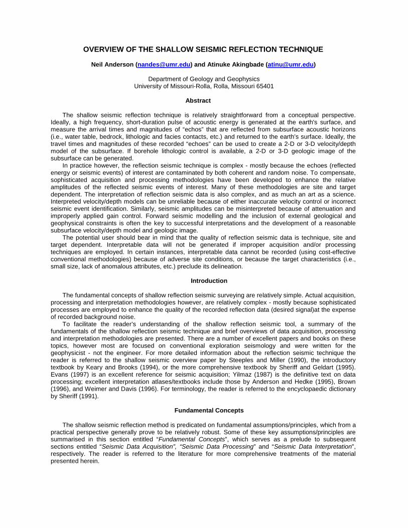
Assumption/principle 1: The shallow subsurface of the earth can be subdivided into a finite number of layers of uniform (or uniformly varying) density and seismic velocity (Figure 1). The water table, bedrock surface, lithologic contacts and/or unconformable surfaces separate these layers. (Note: seismic velocity is a function of density and elastic moduli. The product of velocity and density is referred to as acoustic impedance.)

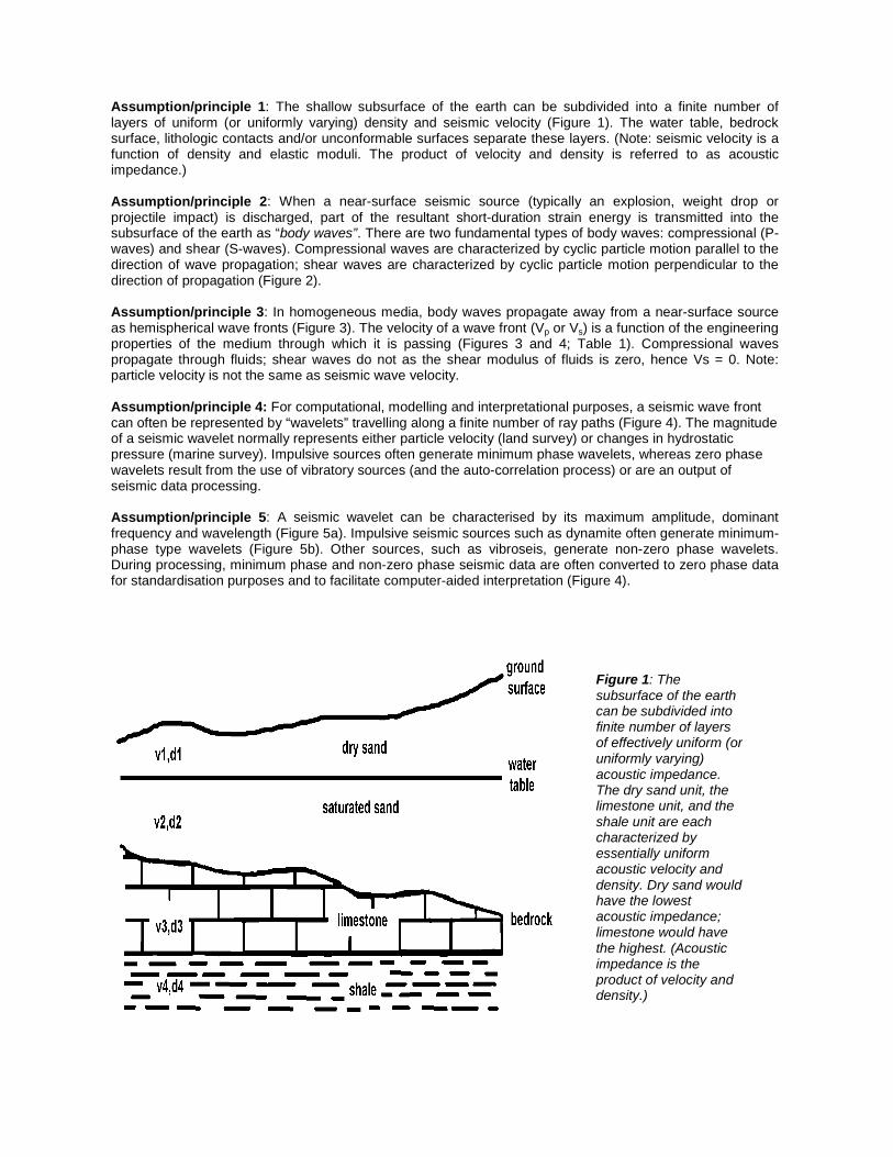
Assumption/principle 2: When a near-surface seismic source (typically an explosion, weight drop or projectile impact) is discharged, part of the resultant short-duration strain energy is transmitted into the subsurface of the earth as “body waves”. There are two fundamental types of body waves: compressional (P-waves) and shear (S-waves). Compressional waves are characterized by cyclic particle motion parallel to the direction of wave propagation; shear waves are characterized by cyclic particle motion perpendicular to the direction of propagation (Figure 2).

Assumption/principle 3: In homogeneous media, body waves propagate away from a near-surface source as hemispherical wave fronts (Figure 3). The velocity of a wave front (Vp or Vs) is a function of the engineering properties of the medium through which it is passing (Figures 3 and 4; Table 1). Compressional waves propagate through fluids; shear waves do not as the shear modulus of fluids is zero, hence Vs = 0. Note: particle velocity is not the same as seismic wave velocity.

Assumption/principle 4: For computational, modelling and interpretational purposes, a seismic wave front can often be represented by “wavelets” travelling along a finite number of ray paths (Figure 4). The magnitude of a seismic wavelet normally represents either particle velocity (land survey) or changes in hydrostatic pressure (marine survey). Impulsive sources often generate minimum phase wavelets, whereas zero phase wavelets result from the use of vibratory sources (and the auto-correlation process) or are an output of seismic data processing.

Assumption/principle 5: A seismic wavelet can be characterised by its maximum amplitude, dominant frequency and wavelength (Figure 5a). Impulsive seismic sources such as dynamite often generate minimum-phase type wavelets (Figure 5b). Other sources, such as vibroseis, generate non-zero phase wavelets. During processing, minimum phase and non-zero phase seismic data are often converted to zero phase data for standardisation purposes and to facilitate computer-aided interpretation (Figure 4).

Figure 1: The subsurface of the earth can be subdivided into finite number of layers of effectively uniform (or uniformly varying) acoustic impedance. The dry sand unit, the limestone unit, and the shale unit are each characterized by essentially uniform acoustic velocity and density. Dry sand would have the lowest acoustic impedance; limestone would have the highest. (Acoustic impedance is the product of velocity and density.)

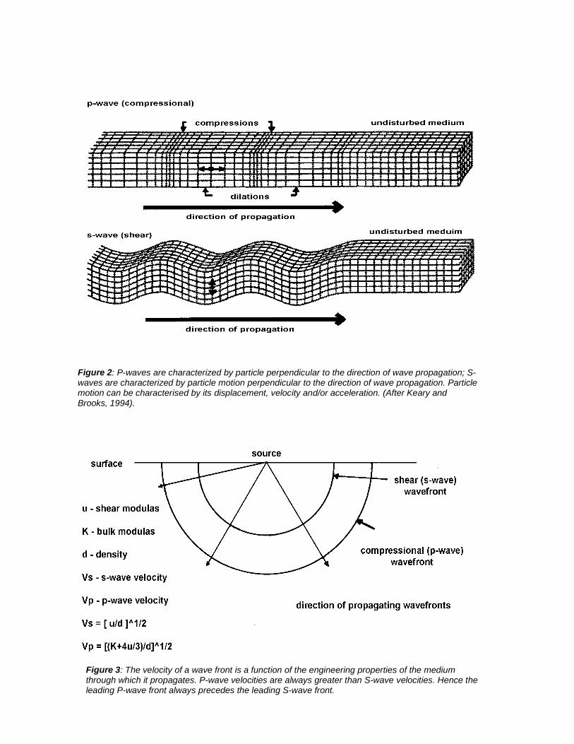
Figure 2: P-waves are characterized by particle perpendicular to the direction of wave propagation; S-waves are characterized by particle motion perpendicular to the direction of wave propagation. Particle motion can be characterised by its displacement, velocity and/or acceleration. (After Keary and Brooks, 1994).

Figure 3: The velocity of a wave front is a function of the engineering properties of the medium through which it propagates. P-wave velocities are always greater than S-wave velocities. Hence the leading P-wave front always precedes the leading S-wave front.

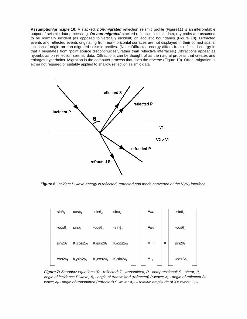
Assumption/principle 6: When seismic energy is incident on a subsurface interface across which there is a change in acoustic impedance, energy will be reflected and refracted (transmitted) in accordance with Snell’s law (Figure 6). Mode conversion (P-wave to S-wave or vice-versa) will also occur. The angles of the incident, reflected and refracted modes can be calculated using the following equation:

Sin θ1/V1 = Sin θ2/V2 = Sin θ3/V3

Where θ1 is the angle of incidence; V1 is the velocity of the incident ray; θ2 is the angle of reflection; V2 is the velocity of the reflected ray; θ3 is the angle of refraction; and V3 is the velocity of the refracted ray.

Assumption/principle 7: The relative magnitudes of the reflected and transmitted wavelets can be calculated from the Zoeppritz equations (derived assuming conservation of particle displacement and stress; Figure 7). Generally, for modelling, processing and interpretation purposes, near-vertical incidence is assumed, and the relative magnitudes of the reflected and transmitted wavelets are estimated using the equations shown in Figure 8.

Assumption/principle 8: The amplitudes of recorded wavelets are functions of both the reflection coefficients of the reflecting horizons (Figures 7 and 8) and transmission losses (Figure 9). During seismic data processing, the amplitudes of recorded wavelets are modified (gained) in an attempt to compensate for transmission losses. Hence, on ideally processed reflection seismic data, wavelet amplitudes are a direct function of the corresponding reflection coefficients.

Assumption/principle 9: A stacked, migrated reflection seismic profile (Figure 10) is an interpretable output of seismic data processing. A migrated reflection seismic profile is comprised of a suite of individual traces, each placed at its surface (CMP) location of origin. The spacing between adjacent traces represents the horizontal control interval as established by field acquisition parameters. Migrated reflected seismic data have been modified such that the ray paths appear to have been both vertical (as though acquired using coincident source/receiver pair located at the CMP) and normally incident on reflecting surfaces (in spite of actual subsurface geometries). Hence, the relative magnitude of seismic wavelets can be calculated using the equation in Figure 8. On migrated seismic profiles, acoustic impedance interfaces are essentially “replaced” in time by wavelets. The two-way travel time to a seismic event is a direct function of the vertical depth to the horizon of origin and the magnitude of the wavelet is a direct function of the magnitude of the corresponding vertical incident reflection coefficient

Material P-wave

Velocity (km/s)

Dry Sand 0.2 -.0.1 Wet Sand 1.5 - 2.0

Clay 1.0 - 2.5 Permafrost 3.5 - 4.0

Tertiary Sandstone 2.0 - 2.5 Pennant Sandstone 4.0 - 4.5 Cambrian Quartzite 5.5 - 6.0

Cretaceous Limestone 2.0 - 2.5 Carboniferous Limestone 5.0 - 5.5

Dolomites 2.5 - 6.5

P-wave Material Velocity

(Km/s)

Rock Salt 4.5 - 5.0 Anhydrite 4.5 - 6.5 Gypsum 2.0 - 3.5 Granite 5.5 - 6.0 Gabbro 6.5 - 7.0

Ultramafic Rocks 7.5 - 8.5 Air 0.3

Water 1.4 - 1.5 Ice 3.4

Petroleum 1.3 -1.4

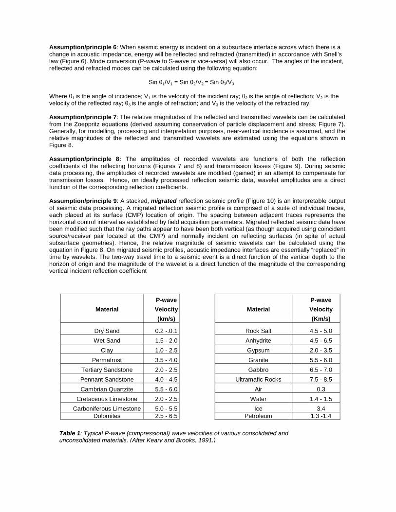
Table 1: Typical P-wave (compressional) wave velocities of various consolidated and unconsolidated materials. (After Keary and Brooks, 1991.)

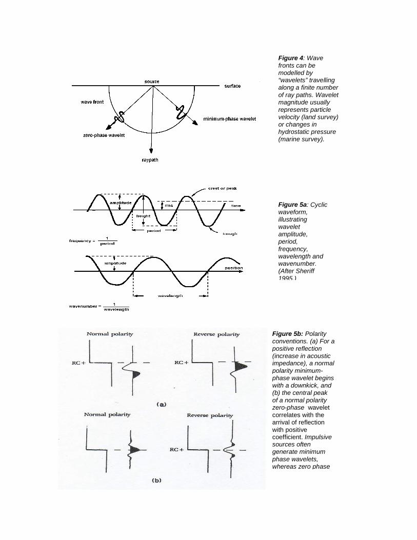
Figure 4: Wave fronts can be modelled by “wavelets” travelling along a finite number of ray paths. Wavelet magnitude usually represents particle velocity (land survey) or changes in hydrostatic pressure (marine survey).

Figure 5a: Cyclic waveform, illustrating wavelet amplitude, period, frequency, wavelength and wavenumber. (After Sheriff 1995.)

Figure 5b: Polarity conventions. (a) For a positive reflection (increase in acoustic impedance), a normal polarity minimum-phase wavelet begins with a downkick, and (b) the central peak of a normal polarity zero-phase wavelet correlates with the arrival of reflection with positive coefficient. Impulsive sources often generate minimum phase wavelets, whereas zero phase

Assumption/principle 10: A stacked, non-migrated reflection seismic profile (Figure11) is an interpretable output of seismic data processing. On non-migrated stacked reflection seismic data, ray paths are assumed to be normally incident (as opposed to vertically incident) on acoustic boundaries (Figure 10). Diffracted events and reflected events originating from non-horizontal surfaces are not displayed in their correct spatial location of origin on non-migrated seismic profiles. {Note: Diffracted energy differs from reflected energy in that it originates from “point source discontinuities”, rather than reflective interfaces.} Diffractions appear as hyperbolas on reflection seismic data. Diffractions can be thought of as the natural process that creates and enlarges hyperbolas. Migration is the computer process that does the reverse (Figure 10). Often, migration is either not required or suitably applied to shallow reflection seismic data.

Figure 6: Incident P-wave energy is reflected, refracted and mode converted at the V1/V2 interface.

Figure 7: Zeoppritz equations (R - reflected; T - transmitted; P - compressional; S - shear; 81 -angle of incidence P-wave; 82 - angle of transmitted (refracted) P-wave; r1 - angle of reflected S-wave; r2 - angle of transmitted (refracted) S-wave; Axy – relative amplitude of XY event; Kn –

sin 1 cos 1 -sin 2 sin 2 ARP -sin 1

-cos 1 sin 1 -cos 2 -sin 2 ARS -cos 1

sin2 1 K1cos2 1 K2sin2 2 K3cos2 2 ATP = sin2 1

cos2 1 K4sin2 2 K5cos2 2 K6sin2 2 ATS -cos2 1

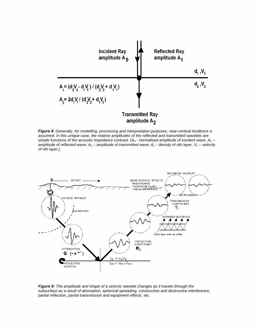
Figure 8: Generally, for modelling, processing and interpretation purposes, near-vertical incidence is assumed. In this unique case, the relative amplitudes of the reflected and transmitted wavelets are simple functions of the acoustic impedance contrast. (A0 - normalised amplitude of incident wave, A1 – amplitude of reflected wave; A2 – amplitude of transmitted wave; dn – density of nth layer; Vn – velocity of nth layer.)

Figure 9: The amplitude and shape of a seismic wavelet changes as it travels through the subsurface as a result of absorption, spherical spreading, constructive and destructive interference, partial reflection, partial transmission and equipment effects, etc.

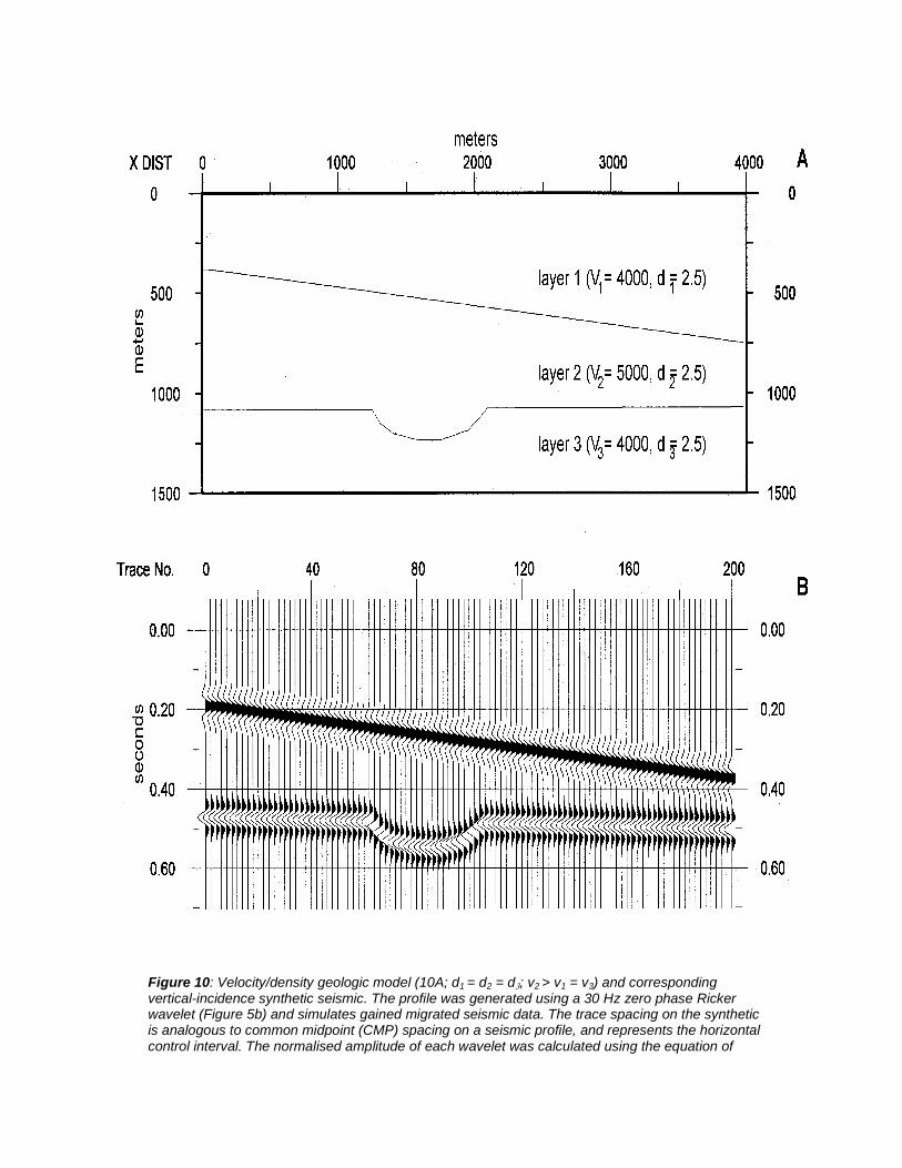
Figure 10: Velocity/density geologic model (10A; d1 = d2 = d3; v2 > v1 = v3) and corresponding vertical-incidence synthetic seismic. The profile was generated using a 30 Hz zero phase Ricker wavelet (Figure 5b) and simulates gained migrated seismic data. The trace spacing on the synthetic is analogous to common midpoint (CMP) spacing on a seismic profile, and represents the horizontal control interval. The normalised amplitude of each wavelet was calculated using the equation of

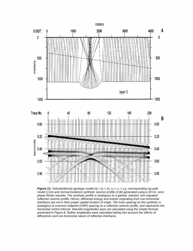
Figure 11: Velocity/density geologic model (d = d2 = d3; v 2 > v1 = v3), corresponding ray path model (11A) and normal-incidence synthetic seismic profile (11B) generated using a 30 Hz, zero-phase Ricker wavelet. The synthetic profile is analogous to a gained, stacked, non-migrated reflection seismic profile. Hence, diffracted energy and events originating from non-horizontal interfaces are not in their proper spatial location of origin. The trace spacing on the synthetic is analogous to common midpoint (CMP) spacing on a reflection seismic profile, and represents the horizontal control interval. Wavelet magnitudes were not calculated using the simple formula presented in Figure 8. Rather amplitudes were calculated taking into account the effects of diffractions and non-horizontal nature of reflective interfaces.

Seismic Data Acquisition

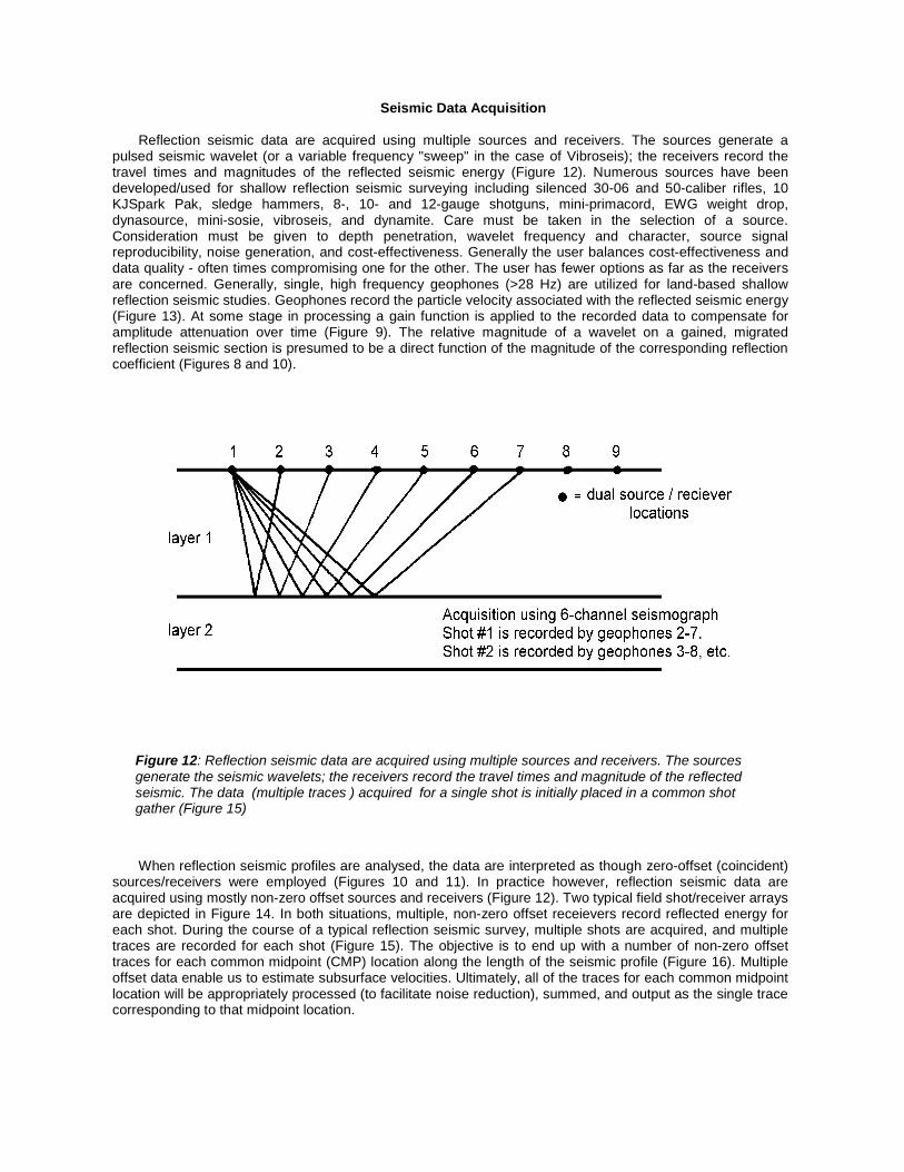
Reflection seismic data are acquired using multiple sources and receivers. The sources generate a pulsed seismic wavelet (or a variable frequency "sweep" in the case of Vibroseis); the receivers record the travel times and magnitudes of the reflected seismic energy (Figure 12). Numerous sources have been developed/used for shallow reflection seismic surveying including silenced 30-06 and 50-caliber rifles, 10 KJSpark Pak, sledge hammers, 8-, 10- and 12-gauge shotguns, mini-primacord, EWG weight drop, dynasource, mini-sosie, vibroseis, and dynamite. Care must be taken in the selection of a source. Consideration must be given to depth penetration, wavelet frequency and character, source signal reproducibility, noise generation, and cost-effectiveness. Generally the user balances cost-effectiveness and data quality - often times compromising one for the other. The user has fewer options as far as the receivers are concerned. Generally, single, high frequency geophones (>28 Hz) are utilized for land-based shallow reflection seismic studies. Geophones record the particle velocity associated with the reflected seismic energy (Figure 13). At some stage in processing a gain function is applied to the recorded data to compensate for amplitude attenuation over time (Figure 9). The relative magnitude of a wavelet on a gained, migrated reflection seismic section is presumed to be a direct function of the magnitude of the corresponding reflection coefficient (Figures 8 and 10).

Figure 12: Reflection seismic data are acquired using multiple sources and receivers. The sources generate the seismic wavelets; the receivers record the travel times and magnitude of the reflected seismic. The data (multiple traces ) acquired for a single shot is initially placed in a common shot gather (Figure 15)

When reflection seismic profiles are analysed, the data are interpreted as though zero-offset (coincident) sources/receivers were employed (Figures 10 and 11). In practice however, reflection seismic data are acquired using mostly non-zero offset sources and receivers (Figure 12). Two typical field shot/receiver arrays are depicted in Figure 14. In both situations, multiple, non-zero offset receievers record reflected energy for each shot. During the course of a typical reflection seismic survey, multiple shots are acquired, and multiple traces are recorded for each shot (Figure 15). The objective is to end up with a number of non-zero offset traces for each common midpoint (CMP) location along the length of the seismic profile (Figure 16). Multiple offset data enable us to estimate subsurface velocities. Ultimately, all of the traces for each common midpoint location will be appropriately processed (to facilitate noise reduction), summed, and output as the single trace corresponding to that midpoint location.

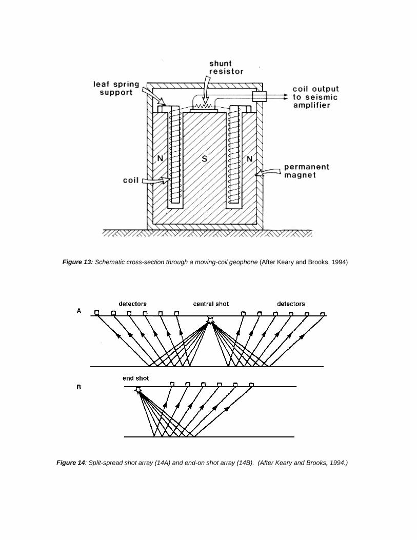
Figure 13: Schematic cross-section through a moving-coil geophone (After Keary and Brooks, 1994)

Figure 14: Split-spread shot array (14A) and end-on shot array (14B). (After Keary and Brooks, 1994.)

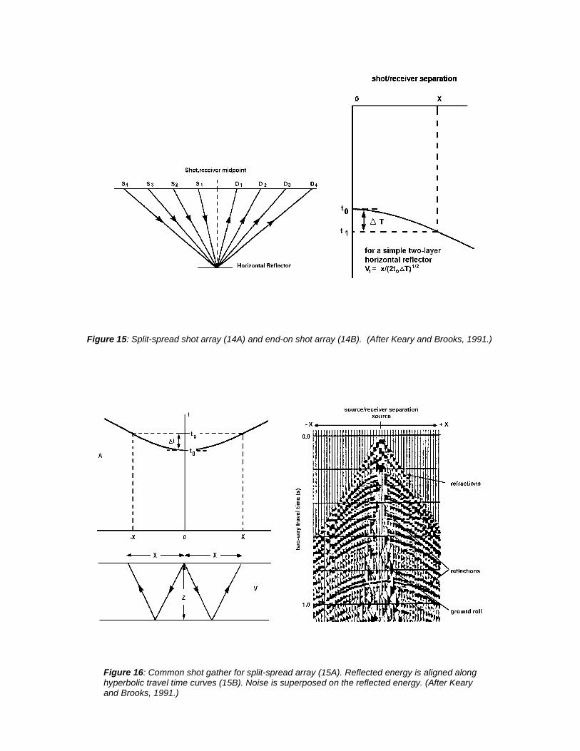
Figure 15: Split-spread shot array (14A) and end-on shot array (14B). (After Keary and Brooks, 1991.)

Figure 16: Common shot gather for split-spread array (15A). Reflected energy is aligned along hyperbolic travel time curves (15B). Noise is superposed on the reflected energy. (After Keary and Brooks, 1991.)

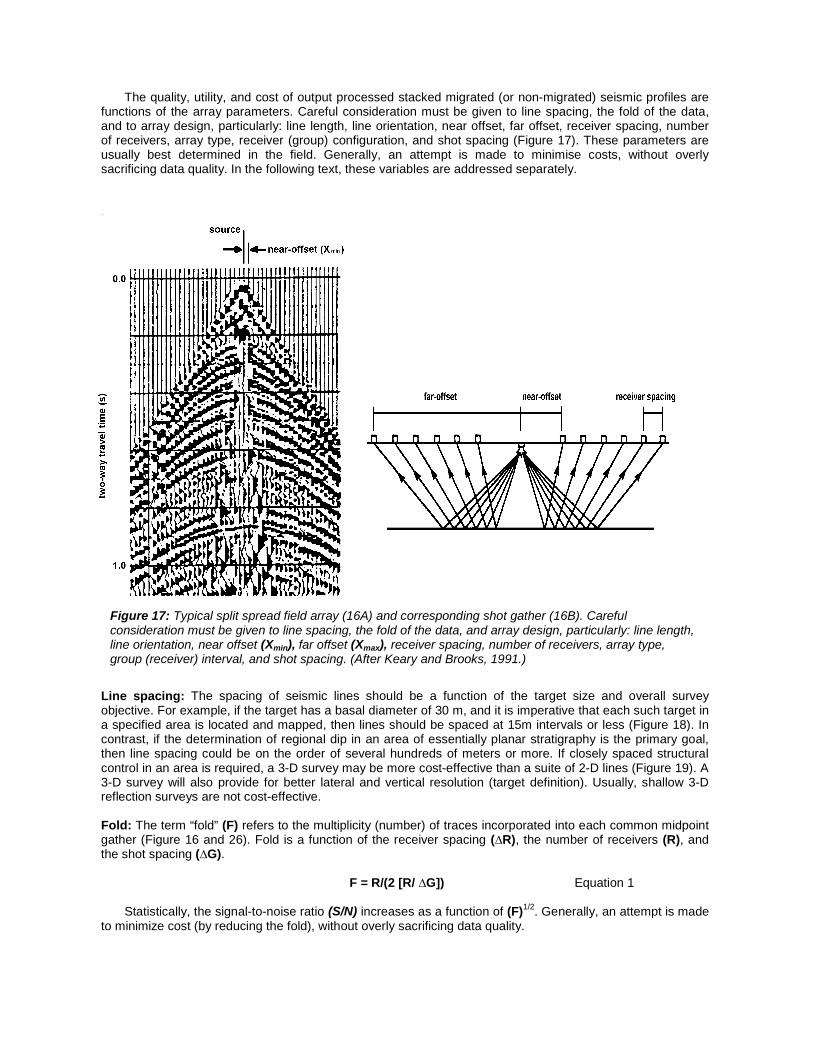
The quality, utility, and cost of output processed stacked migrated (or non-migrated) seismic profiles are functions of the array parameters. Careful consideration must be given to line spacing, the fold of the data, and to array design, particularly: line length, line orientation, near offset, far offset, receiver spacing, number of receivers, array type, receiver (group) configuration, and shot spacing (Figure 17). These parameters are usually best determined in the field. Generally, an attempt is made to minimise costs, without overly sacrificing data quality. In the following text, these variables are addressed separately.

Figure 17: Typical split spread field array (16A) and corresponding shot gather (16B). Careful consideration must be given to line spacing, the fold of the data, and array design, particularly: line length, line orientation, near offset (Xmin), far offset (Xmax), receiver spacing, number of receivers, array type, group (receiver) interval, and shot spacing. (After Keary and Brooks, 1991.)

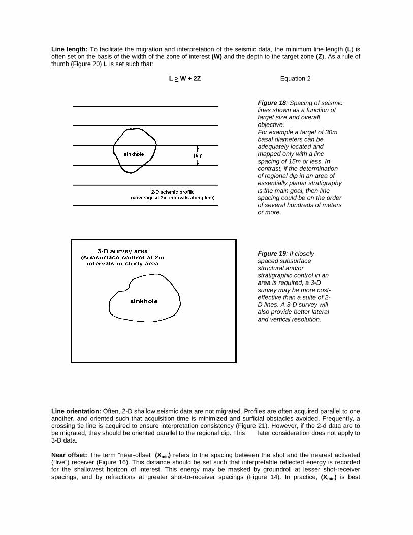
Line spacing: The spacing of seismic lines should be a function of the target size and overall survey objective. For example, if the target has a basal diameter of 30 m, and it is imperative that each such target in a specified area is located and mapped, then lines should be spaced at 15m intervals or less (Figure 18). In contrast, if the determination of regional dip in an area of essentially planar stratigraphy is the primary goal, then line spacing could be on the order of several hundreds of meters or more. If closely spaced structural control in an area is required, a 3-D survey may be more cost-effective than a suite of 2-D lines (Figure 19). A 3-D survey will also provide for better lateral and vertical resolution (target definition). Usually, shallow 3-D reflection surveys are not cost-effective.

Fold: The term “fold” (F) refers to the multiplicity (number) of traces incorporated into each common midpoint gather (Figure 16 and 26). Fold is a function of the receiver spacing (∆R), the number of receivers (R), and the shot spacing (∆G).

F = R/(2 [R/ ∆G]) Equation 1

Statistically, the signal-to-noise ratio (S/N) increases as a function of (F)1/2. Generally, an attempt is made to minimize cost (by reducing the fold), without overly sacrificing data quality.

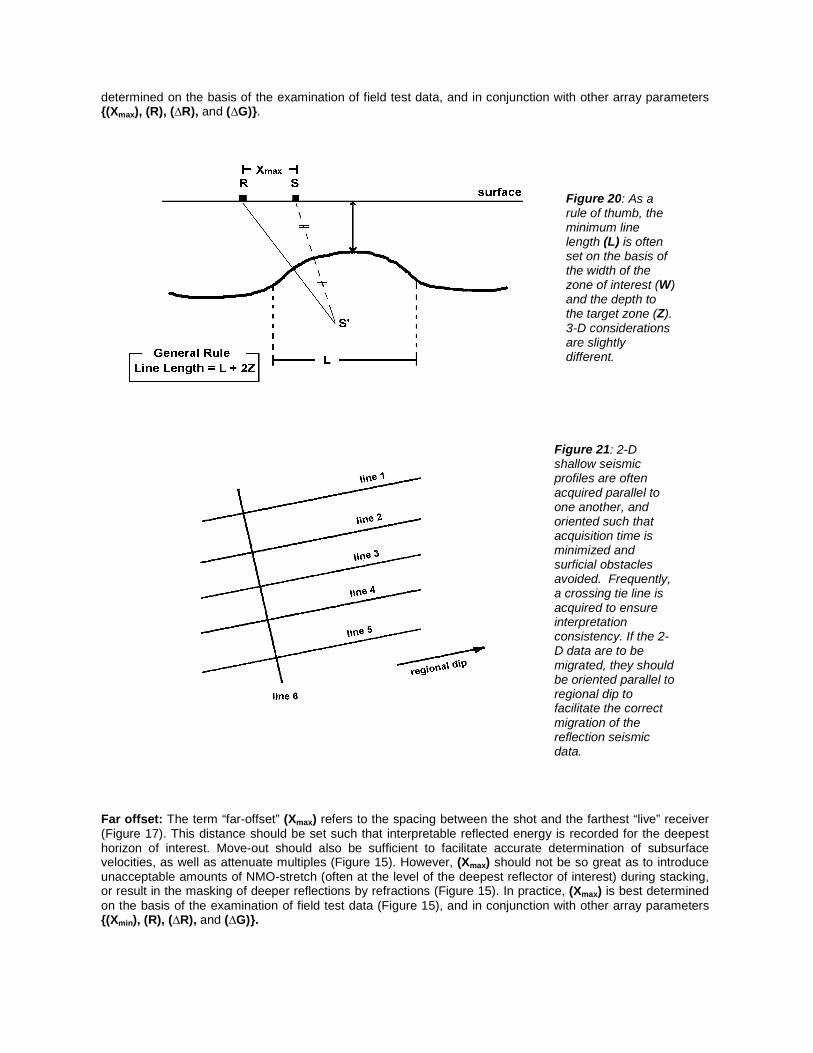
Line length: To facilitate the migration and interpretation of the seismic data, the minimum line length (L) is often set on the basis of the width of the zone of interest (W) and the depth to the target zone (Z). As a rule of thumb (Figure 20) L is set such that:

L > W + 2Z Equation 2

Figure 18: Spacing of seismic lines shown as a function of target size and overall objective. For example a target of 30m basal diameters can be adequately located and mapped only with a line spacing of 15m or less. In contrast, if the determination of regional dip in an area of essentially planar stratigraphy is the main goal, then line spacing could be on the order of several hundreds of meters or more.

Figure 19: If closely spaced subsurface structural and/or stratigraphic control in an area is required, a 3-D survey may be more cost-effective than a suite of 2-D lines. A 3-D survey will also provide better lateral and vertical resolution.

Line orientation: Often, 2-D shallow seismic data are not migrated. Profiles are often acquired parallel to one another, and oriented such that acquisition time is minimized and surficial obstacles avoided. Frequently, a crossing tie line is acquired to ensure interpretation consistency (Figure 21). However, if the 2-d data are to be migrated, they should be oriented parallel to the regional dip. This later consideration does not apply to 3-D data.

Near offset: The term “near-offset” (Xmin) refers to the spacing between the shot and the nearest activated (“live”) receiver (Figure 16). This distance should be set such that interpretable reflected energy is recorded for the shallowest horizon of interest. This energy may be masked by groundroll at lesser shot-receiver spacings, and by refractions at greater shot-to-receiver spacings (Figure 14). In practice, (Xmin) is best

determined on the basis of the examination of field test data, and in conjunction with other array parameters {(Xmax), (R), (∆R), and (∆G)}.

Figure 20: As a rule of thumb, the minimum line length (L) is often set on the basis of the width of the zone of interest (W) and the depth to the target zone (Z). 3-D considerations are slightly different.

Figure 21: 2-D shallow seismic profiles are often acquired parallel to one another, and oriented such that acquisition time is minimized and surficial obstacles avoided. Frequently, a crossing tie line is acquired to ensure interpretation consistency. If the 2-D data are to be migrated, they should be oriented parallel to regional dip to facilitate the correct migration of the reflection seismic data.

Far offset: The term “far-offset” (Xmax) refers to the spacing between the shot and the farthest “live” receiver (Figure 17). This distance should be set such that interpretable reflected energy is recorded for the deepest horizon of interest. Move-out should also be sufficient to facilitate accurate determination of subsurface velocities, as well as attenuate multiples (Figure 15). However, (Xmax) should not be so great as to introduce unacceptable amounts of NMO-stretch (often at the level of the deepest reflector of interest) during stacking, or result in the masking of deeper reflections by refractions (Figure 15). In practice, (Xmax) is best determined on the basis of the examination of field test data (Figure 15), and in conjunction with other array parameters {(Xmin), (R), (∆R), and (∆G)}.

Receiver spacing: (.R): Refers to the distance between adjacent geophones (or groups of geophones; Figure 17). Generally, subsurface coverage (trace spacing on seismic profile; Figure 10) is ½ ∆R, and should be sufficiently small to avoid aliasing. If (R) is fixed by the equipment available; (∆R) is a direct function of (Xmin) and (Xmax)

Number of receivers: The number of “live” receivers (R; Figure 12) is usually a fixed function of the equipment used (i.e., 12-channel seismograph, 24-channel seismograph, 48-channel seismograph, etc.). However, if options are available, R should be determined on the basis of (∆R), (Xmin) and (Xmax).

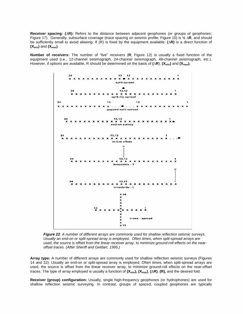
Figure 22: A number of different arrays are commonly used for shallow reflection seismic surveys. Usually an end-on or split-spread array is employed. Often times, when split-spread arrays are used, the source is offset from the linear receiver array, to minimize ground-roll effects on the near-offset traces. (After Sheriff and Geldart, 1995.)

Array type: A number of different arrays are commonly used for shallow reflection seismic surveys (Figures 14 and 22). Usually an end-on or split-spread array is employed. Often times, when split-spread arrays are used, the source is offset from the linear receiver array, to minimize ground-roll effects on the near-offset traces. The type of array employed is usually a function of (Xmin), (Xmax), (.R), (R), and the desired fold.

Receiver (group) configuration: Usually, single high-frequency geophones (or hydrophones) are used for shallow reflection seismic surveying. In contrast, groups of spaced, coupled geophones are typically

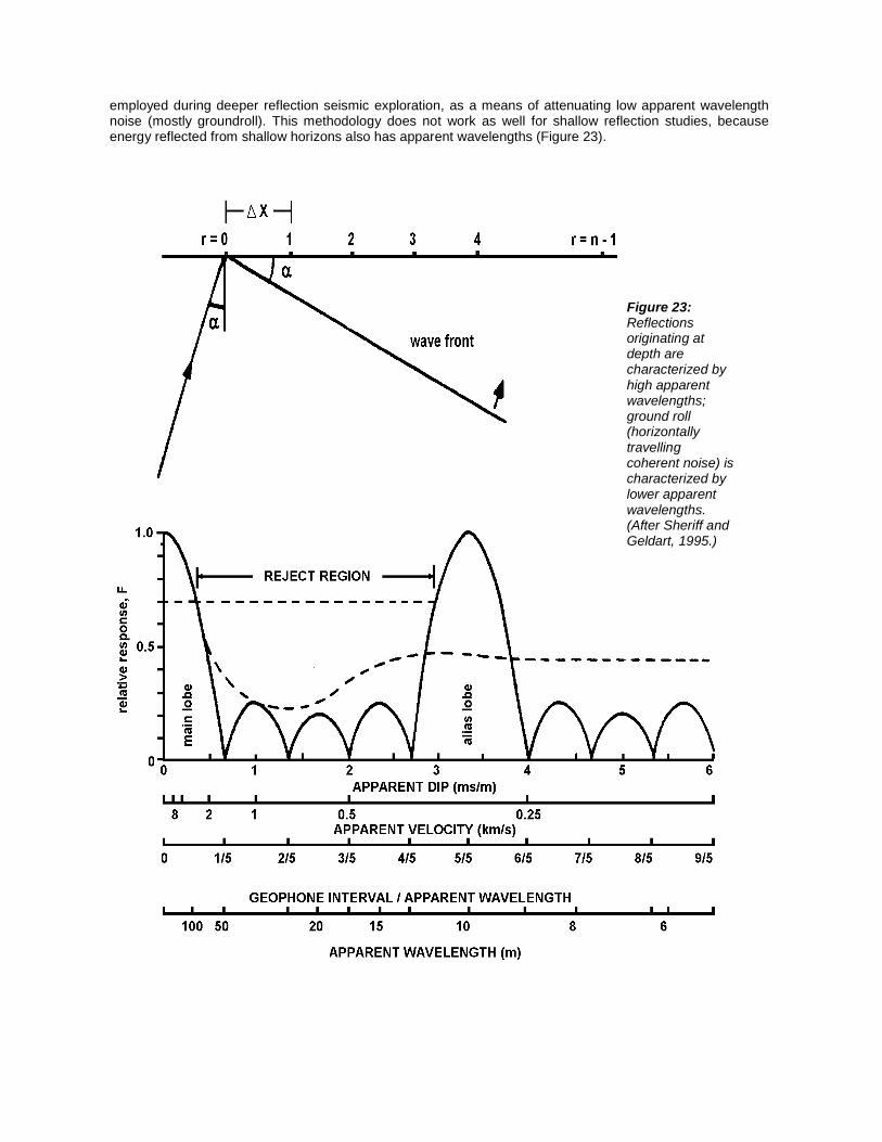
employed during deeper reflection seismic exploration, as a means of attenuating low apparent wavelength noise (mostly groundroll). This methodology does not work as well for shallow reflection studies, because energy reflected from shallow horizons also has apparent wavelengths (Figure 23).

Figure 23: Reflections originating at depth are characterized by high apparent wavelengths; ground roll (horizontally travelling coherent noise) is characterized by lower apparent wavelengths. (After Sheriff and Geldart, 1995.)

Processing

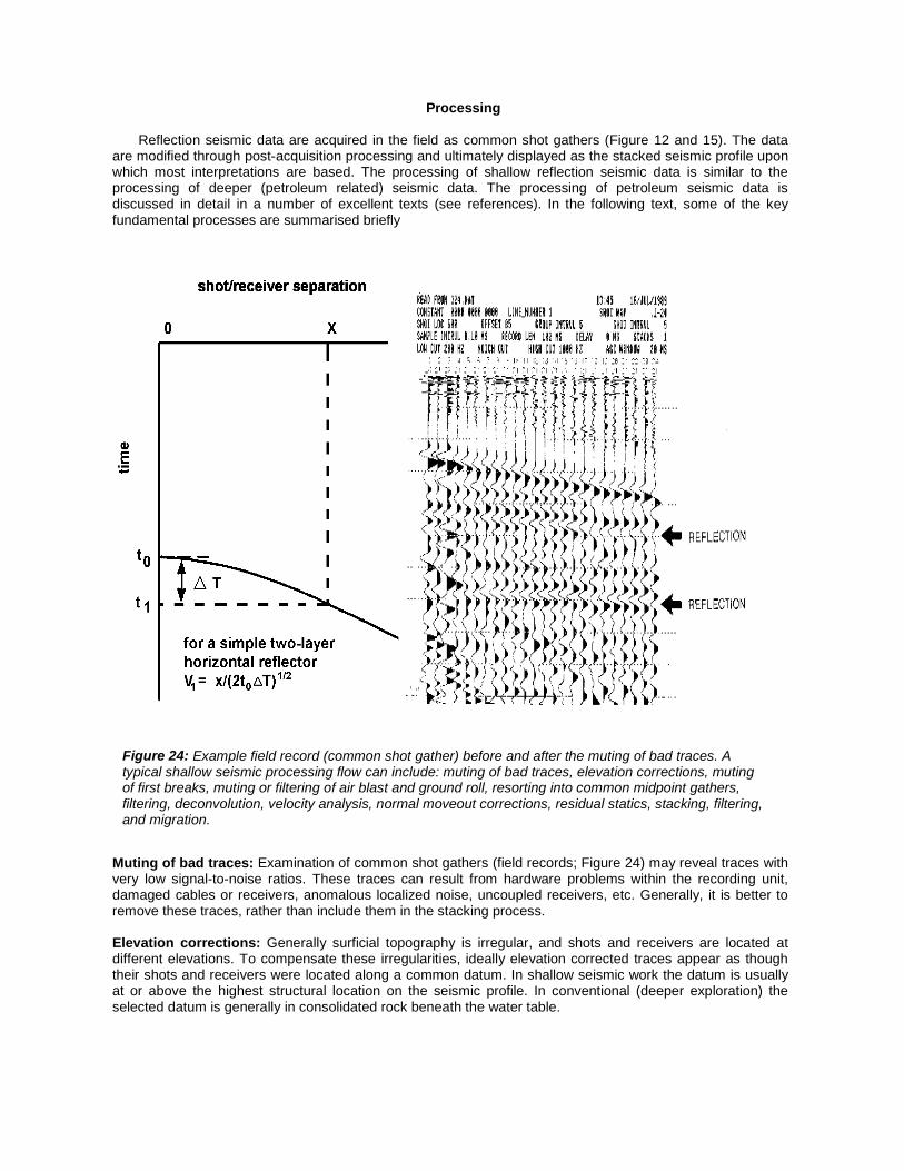
Reflection seismic data are acquired in the field as common shot gathers (Figure 12 and 15). The data are modified through post-acquisition processing and ultimately displayed as the stacked seismic profile upon which most interpretations are based. The processing of shallow reflection seismic data is similar to the processing of deeper (petroleum related) seismic data. The processing of petroleum seismic data is discussed in detail in a number of excellent texts (see references). In the following text, some of the key fundamental processes are summarised briefly

Figure 24: Example field record (common shot gather) before and after the muting of bad traces. A typical shallow seismic processing flow can include: muting of bad traces, elevation corrections, muting of first breaks, muting or filtering of air blast and ground roll, resorting into common midpoint gathers, filtering, deconvolution, velocity analysis, normal moveout corrections, residual statics, stacking, filtering, and migration.

Muting of bad traces: Examination of common shot gathers (field records; Figure 24) may reveal traces with very low signal-to-noise ratios. These traces can result from hardware problems within the recording unit, damaged cables or receivers, anomalous localized noise, uncoupled receivers, etc. Generally, it is better to remove these traces, rather than include them in the stacking process.

Elevation corrections: Generally surficial topography is irregular, and shots and receivers are located at different elevations. To compensate these irregularities, ideally elevation corrected traces appear as though their shots and receivers were located along a common datum. In shallow seismic work the datum is usually at or above the highest structural location on the seismic profile. In conventional (deeper exploration) the selected datum is generally in consolidated rock beneath the water table.

Muting of first breaks: Refractions are generally considered to be noise, and are generally muted (Figure 15b). Refracted acoustic energy has been critically refracted along acoustic impedance interfaces, and constitutes noise on reflection seismic data.

Muting or filtering of air blast and ground roll: Air blast is acoustic energy that has travelled from the source to the receivers through air. Ground roll consists of low-velocity, surface-guided acoustic energy (similar to particle motion in oceanic swells). Both air blast and ground roll are considered to be noise, and are filtered or muted (Figure 15b). F/K filters can be used to remove this coherent noise on the basis of its low apparent short wavelength, or long high apparent wave number (Sheriff and Geldart, 1995.).

Filtering: Data can be filtered at any step in the processing sequence (Figure 25). Data may be filtered to remove undesired frequency components (time or frequency domain filters), or to remove a range of undesired apparent wave numbers (F/K filtering; Sheriff and Geldart, 1995).

Deconvolution: Deconvolution is applied to shallow seismic data generally as a means of enhancing the higher frequency components of the recorded signal, or transforming a non-zero phase data into zero-phase data. Effective deconvolution operators can be difficult to design (because of variable source signatures, short trace lengths, and high attenuation in the shallow subsurface). Deconvolution can be more destructive than constructive in many circumstances (re: quality of the output signal). Data can be deconvolved both before and/or after stacking.

Velocity analysis: Velocity analysis can be done on either common shot gathered data or common midpoint data. Subsurface interval and root mean square (RMS) velocities can be determined sequentially for the shallowest through deepest reflectors on the basis of the analysis of their respective hyperbolic travel time curves.

Resorting into common midpoint gathers: Prior to stacking, the reflection seismic traces are resorted into common midpoint gathers (Figures 16 and 26). All of the traces in a common midpoint gather are assumed to have common subsurface reflection points.

Normal moveout corrections: Normal move out (NMO) corrections are applied to common midpoint data. Primary reflected energy is horizontally aligned on NMO corrected gathers (Figure 25). In areas of complex subsurface structure Dip move out (DMO) corrections may be applied.

Residual statics: Automatic statics are generally applied to the NMO-corrected common midpoint gathers. The intent is to statistically align the reflected energy and improve the quality of the output stacked data.

Stacking: All of the traces in each NMO corrected common midpoint (CMP) gather are summed together, and output as a single trace. All of these traces are plotted at their corresponding CMP locations on the output stacked seismic profile (Figures 25 and 27).

Migration: Dipping reflections are not properly located (spatially) on the output stacked seismic section unless migration has been applied. Migration effectively shifts seismic reflection energy (including diffractions) to its spatial point of origin (Figure 11and 28). In practice however, it is usually not cost-effective to acquire shallow reflection data that is suitable (re: array considerations) for migration, and generally, acceptable interpretations can be done on non-migrated data. Problems also arise because migration of 2-D profile data will not properly shift dipping events unless the profile is oriented parallel to dip; neither will it properly migrate energy that originates out of the plane of the seismic profile. These problems can be overcome by acquiring 3-D reflection seismic data. However, shallow 3-D reflection seismic surveying is usually not cost-effective.

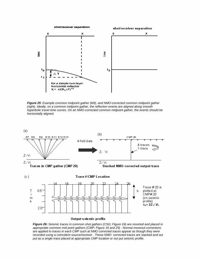
Figure 25: Example common midpoint gather (left), and NMO-corrected common midpoint gather (right). Ideally, on a common midpoint gather, the reflection events are aligned along smooth hyperbolic travel time curves. On an NMO-corrected common midpoint gather, the events should be horizontally aligned.

Figure 26: Seismic traces in common shot gathers (CSG; Figure 24) are resorted and placed in appropriate common mid point gathers (CMP; Figure 16 and 25) . Normal moveout corrections are applied to traces in each CMP such at NMO corrected traces appear as though they were recorded using a coincident source/receiver . These NMO corrected traces are stacked and out put as a single trace placed at appropriate CMP location or out put seismic profile.

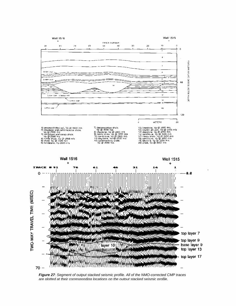
Figure 27: Segment of output stacked seismic profile. All of the NMO-corrected CMP traces are plotted at their corresponding locations on the output stacked seismic profile.

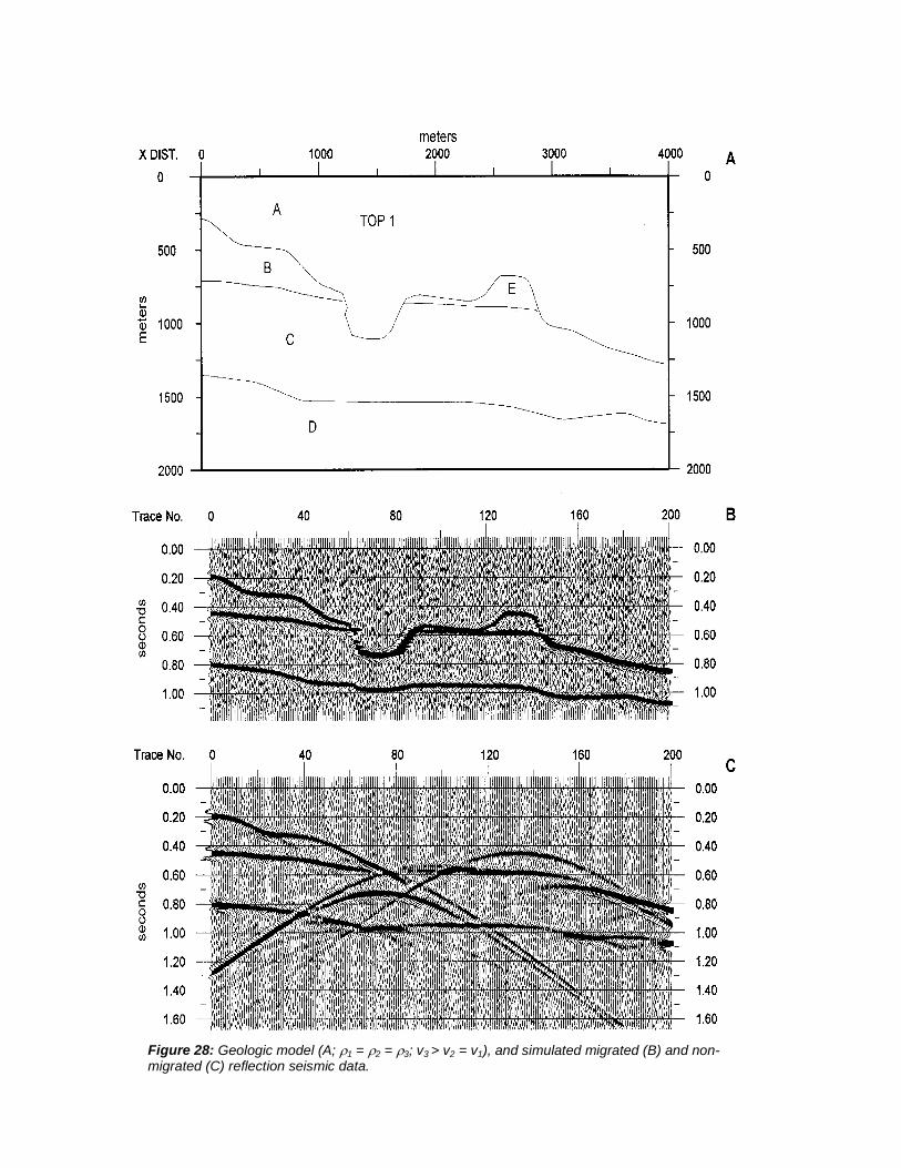
Figure 28: Geologic model (A; p1 = p2 = p3; v3 > v2 = v1), and simulated migrated (B) and non-migrated (C) reflection seismic data.

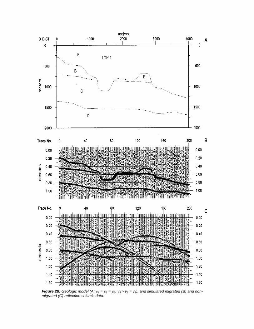
Figure 28: Geologic model (A; p1 = p2 = p3; v3 > v2 = v1), and simulated migrated (B) and non-migrated (C) reflection seismic data.

Interpretation

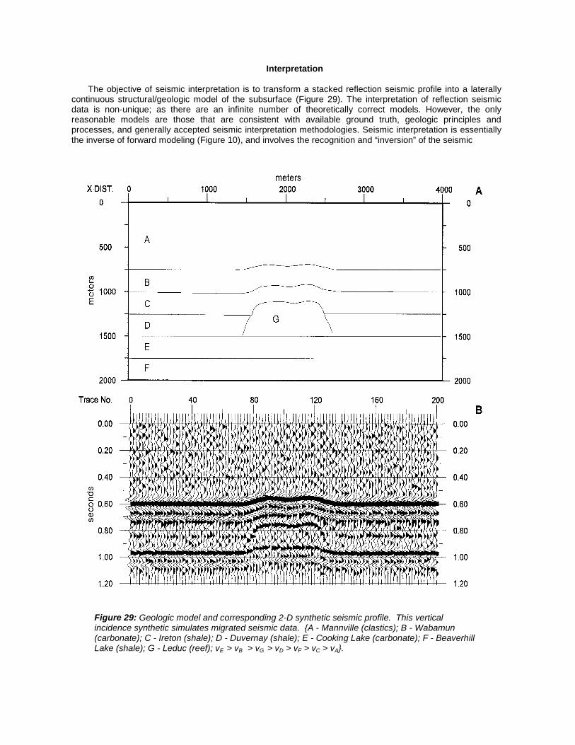
The objective of seismic interpretation is to transform a stacked reflection seismic profile into a laterally continuous structural/geologic model of the subsurface (Figure 29). The interpretation of reflection seismic data is non-unique; as there are an infinite number of theoretically correct models. However, the only reasonable models are those that are consistent with available ground truth, geologic principles and processes, and generally accepted seismic interpretation methodologies. Seismic interpretation is essentially the inverse of forward modeling (Figure 10), and involves the recognition and “inversion” of the seismic

Figure 29: Geologic model and corresponding 2-D synthetic seismic profile. This vertical incidence synthetic simulates migrated seismic data. {A - Mannville (clastics); B - Wabamun (carbonate); C - Ireton (shale); D - Duvernay (shale); E - Cooking Lake (carbonate); F - Beaverhill Lake (shale); G - Leduc (reef); vE > vB > vG > vD > vF > vC > vA}.

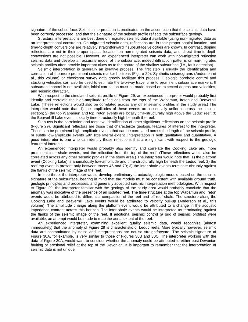
signature of the subsurface. Seismic interpretation is predicated on the assumption that the seismic data have been correctly processed, and that the signature of the seismic profile reflects the subsurface geology.

Structural interpretations are best done on migrated seismic data if available (using non-migrated data as an interpretational constraint). On migrated seismic data, reflections are in their proper spatial location, and time-to-depth conversions are relatively straightforward if subsurface velocities are known. In contrast, dipping reflectors are not in their proper spatial location on non-migrated seismic data, and direct time-to-depth conversions are not possible. However, an experienced interpreter can work with non-migrated reflection seismic data and develop an accurate model of the subsurface; indeed diffraction patterns on non-migrated seismic profiles often provide important clues as to the nature of the shallow subsurface (i.e., fault detection).

Seismic interpretation is generally an iterative process. The first step is usually the identification and correlation of the more prominent seismic marker horizons (Figure 29). Synthetic seismograms (Anderson et al., this volume) or checkshot survey data greatly facilitate this process. Geologic borehole control and stacking velocities can also be used to estimate the two-way travel time to prominent subsurface markers. If subsurface control is not available, initial correlation must be made based on expected depths and velocities, and seismic character.

With respect to the simulated seismic profile of Figure 29, an experienced interpreter would probably first identify and correlate the high-amplitude reflections from the tops of the Wabamun, Ireton and Beaverhill Lake. (These reflections would also be correlated across any other seismic profiles in the study area.) The interpreter would note that: 1) the amplitudes of these events are essentially uniform across the seismic section; 2) the top Wabamun and top Ireton events are locally time-structurally high above the Leduc reef; 3) the Beaverhill Lake event is locally time-structurally high beneath the reef.

Step two is the correlation and tentative identification of other significant reflections on the seismic profile (Figure 29). Significant reflectors are those that characterize geologic features of interest to the interpreter. These can be prominent high-amplitude events that can be correlated across the length of the seismic profile, or subtle low-amplitude events with little lateral extent. Interpretation is both qualitative and quantitative. A good interpreter is one who can identify those reflections that are significant with respect to the geologic feature of interests.

An experienced interpreter would probably also identify and correlate the Cooking Lake and more prominent inter-shale events, and the reflection from the top of the reef. (These reflections would also be correlated across any other seismic profiles in the study area.) The interpreter would note that: 1) the platform event (Cooking Lake) is anomalously low-amplitude and time-structurally high beneath the Leduc reef; 2) the reef top event is present only between traces 46 and 70; 3) the inter-shale events terminate abruptly against the flanks of the seismic image of the reef.

In step three, the interpreter would develop preliminary structural/geologic models based on the seismic signature of the subsurface, bearing in mind that the models must be consistent with available ground truth, geologic principles and processes, and generally accepted seismic interpretation methodologies. With respect to Figure 29, the interpreter familiar with the geology of the study area would probably conclude that the anomaly was indicative of the presence of an isolated reef. The time-structure at the top Wabamun and Ireton events would be attributed to differential compaction of the reef and off-reef shale. The structure along the Cooking Lake and Beaverhill Lake events would be attributed to velocity pull-up (Anderson et al., this volume). The amplitude change along the platform event would be attributed to a change in the acoustic impedance contrast across this horizon. The inter-shale events would be interpreted as terminating against the flanks of the seismic image of the reef. If additional seismic control (a grid of seismic profiles) were available, an attempt would be made to map the aerial extent of the reef.

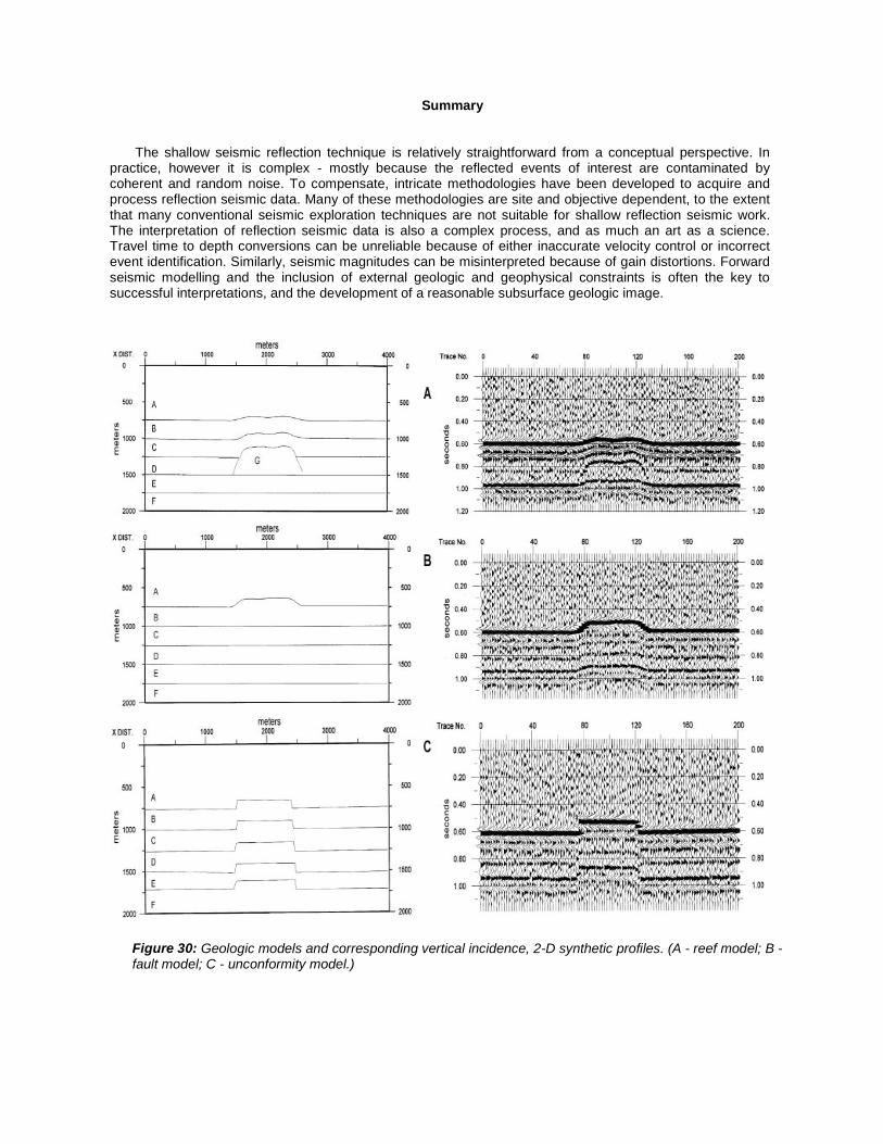
An experienced interpreter, examining excellent quality seismic data, would recognize (almost immediately) that the anomaly of Figure 29 is characteristic of Leduc reefs. More typically however, seismic data are contaminated by noise and interpretations are not so straightforward. The seismic signature of Figure 30A, for example, is very similar to those of Figures 30B and 30C. The interpreter working with the data of Figure 30A, would want to consider whether the anomaly could be attributed to either post-Devonian faulting or erosional relief at the top of the Devonian. It is important to remember that the interpretation of seismic data is not unique!

Summary

The shallow seismic reflection technique is relatively straightforward from a conceptual perspective. In practice, however it is complex - mostly because the reflected events of interest are contaminated by coherent and random noise. To compensate, intricate methodologies have been developed to acquire and process reflection seismic data. Many of these methodologies are site and objective dependent, to the extent that many conventional seismic exploration techniques are not suitable for shallow reflection seismic work. The interpretation of reflection seismic data is also a complex process, and as much an art as a science. Travel time to depth conversions can be unreliable because of either inaccurate velocity control or incorrect event identification. Similarly, seismic magnitudes can be misinterpreted because of gain distortions. Forward seismic modelling and the inclusion of external geologic and geophysical constraints is often the key to successful interpretations, and the development of a reasonable subsurface geologic image.

Figure 30: Geologic models and corresponding vertical incidence, 2-D synthetic profiles. (A - reef model; B -fault model; C - unconformity model.)

References

Anderson, N. L., Cardimona, S., and Roark, M. S., 1998, forward modelling of reflection seismic and ground-penetrating radar signals to aid in field survey design and data interpretation: this volume.

Anderson, N. L., and Hedke, D., Editors, 1995, Geophysical Atlas for Kansas: Kansas Geological Survey Bulletin 237.

Brown, A. R., 1996, Interpretation of three-dimensional seismic data: American Association of Petroleum Geologists Memoir 42, 424 p.

Evans, B. J., 1997, a handbook for seismic data acquisition in exploration: Society of Exploration Geophysicists, 305 p.

Hinds, R., Anderson, N.L., and Kuzmiski, R., 1996, VSP Interpretative Processing: Theory and Practice: Society of Exploration Geophysicists, 205 p.

Keary, P., and Brooks, M., 1991, An Introduction to Geophysical Exploration: Blackwell Scientific Publications, 254 p.

McAnn, D. M., Eddleston, M., Fenning, P. J., and Reeves, G. M., editors, 1997, Modern geophysics in engineering geology: The Geological Society, 441 p.

Sheriff, R. E., 1991, Encyclopedic Dictionary of Exploration Geophysics, Third Edition: Society of Exploration Geophysicists, 376 p.

Sheriff, R. E., and Geldart, L. P., 1995, Exploration Seismology: Press Syndicate of the University of Cambridge, 592 p.

Steeples, D.W. and Miller, R.D., 1990, Seismic reflection methods applied to engineering, environmental and groundwater problems, in Ward, S.H., Editor, Geotechnical and engineering geophysics, volume 1: Society of Exploration Geophysicists, 389 p.

Weimer, P., and Davis, T.L., editors, 1996, Applications of 3-D seismic data to exploration and production: American Association of Petroleum Geologists and Society of Exploration Geophysicists, 270 p.

Yilmaz, O., 1987, Seismic data processing: Society of Exploration Geophysicists, 526 p.