oxidation kinetics of molten copper sulphide

Oxidation Kinetics of Molten Copper Sulphide

By

Abdelmonem Hussein Alyaser

B.Sc. (Metallurgical Engineering), Laurentian University, 1990

A THESIS SUBMITTED IN PARTIAL FULFILLMENT OF

THE REQUIREMENTS FOR THE DEGREE OF

MASTER OF APPLIED SCIENCE

in

THE FACULTY OF GRADUATE STUDIES

(Department of Metals and Materials Engineering)

We accept this thesis as conforming

to the required standard

THE UNIVERSITY OF BRITISH COLUMBIA

July 1993

© Abdelmonem Hussein Alyaser, 1993

In presenting this thesis in partial fulfilment of the requirements for an advanced

degree at the University of British Columbia, I agree that the Library shall make it

freely available for reference and study. I further agree that permission for extensive

copying of this thesis for scholarly purposes may be granted by the head of my

department or by his or her representatives. It is understood that copying or

publication of this thesis for financial gain shall not be allowed without my written

permission.

(Signature)

Department of Metals and Materials Engineering

The University of British ColumbiaVancouver, Canada

Date July 12 1993

DE-6 (2/88)

ABSTRACT

The oxidation kinetics of molten copper sulphide were investigated by quantitative

measurements and qualitative observations. Off-gas analyses for SO2 and 02 were

conducted to determine the oxidation rates of approximately 200-gram samples, of

molten 99.5% Cu2S. The molten sulphide was held in alumina crucibles (approximately

44 mm diameter and 75 mm height), and top-lanced with Ar-02 gas mixtures in the hot

zone of a vertical tube furnace. During the oxidation reaction, gravimetric measurements

of the copper sulphide baths were also conducted to further support the results of the gas

analysis measurements. A series of laboratory tests, involving reaction gas ranging in

composition from 20-78% 02, was conducted to determine the effect of oxygen

concentration on the kinetics of the oxidation reaction. To determine the influence of

volumetric gas flow rate on the kinetics of the oxidation reaction and to study the gas

phase mass transfer, a series of laboratory tests was carried out utilizing a gas flow rate

range of 1-4 liters/min. The effects of other operating conditions, on the oxidation rates,

such as bath mixing, and reaction temperature (1200-1300 °C), were also determined.

The effect of surface-tension driven flow (the Marangoni effect) on the reaction kinetics

was also investigated via surface observation and photography. The overall surface

behavior was monitored for spontaneous motion, and the eruption of gas bubbles from the

melt.

The quantitative analysis of reaction rates was also aided by the micro-examination of

quenched bath samples via optical microscopy. Approximately 4-gram samples were

extracted at specific reaction times, using U-shaped quartz tubes. The samples were

examined microscopically to determine the reaction progress based on the characteristics

of gas bubbles, copper droplets and the phases present.

ii

iii

The oxidation reaction of molten copper sulphide was found to take place in two distinct

kinetic stages. During the primary stage, simultaneous partial desulphurization and

oxygen saturation of the melt, via liquid-gas reaction at the melt surface, takes place.

Upon saturation of the melt with oxygen, the secondary stage immediately commences.

Throughout the secondary stage, the sulphide phase remains at a constant composition

(approximately 80.83 wt% Cu, 17.7 wt% S and 1.47 wt% 0 at 1200 °C and 1 atm), due to

simultaneous surface and melt reactions, until the overall reaction is complete. Three

simultaneous melt reactions occur within the sulphide phase which are responsible for the

formation of the metal phase (approximately 98.89 wt% Cu, 0.95 wt% S and 0.16 wt% 0

at 1200 °C and 1 atm). As a result of settling oxygen- and sulphur-saturated copper

droplets, the metal phase accumulates at the bottom of the bath.

The experimental results revealed that the rate of reaction is controlled by the gas phase

mass transfer of oxygen to the melt surface; the liquid phase mass transfer resistance and

chemical reaction resistance are negligible. The bath was found to be vigorously mixed,

primarily due to the effect of the Marangoni effect although the degree of mixing is

slightly enhanced during the secondary stage as a result of rising SO2 gas bubbles and

falling copper droplets.

Based on the electrochemical behavior of the sulphide melt and the experimental

revelations, a mathematical model was constructed to carry out a fundamental study of

the problem and provide an overall analysis extending beyond the experimental

conditions. The model predictions were found to be in good agreement with the observed

results.

The practical implications of this work are: the copper-making reaction in copper

converting is limited by gas phase mass transfer; in the Peirce-Smith converter, one of the

factors for the high degree of mass transfer in the bath is the effect of surface-tension

driven flows. It is also suggested that the ionic nature of the sulphide bath is another

factor for the low liquid phase mass transfer resistance.

iv

Table of Contents

ABSTRACT^Table of Contents^List of Figures^ viiiList of Tables^ xvList of Symbols^ xixAcknowledgments^ xxiii1. Introduction^ 12. Literature Review^ 4

2.1. Copper Converting^ 42.1.1. History of the Copper Converter^ 42.1.2. Metallurgy of Copper Converting^ 5

2.1.2.1. The Slag-Forming Stage:^ 72.1.2.2. The Copper-Making Stage:^ 7

2.2. Thermodynamics of Copper Sulphide Oxidation^ 82.2.1. Cu-S System^ 92.2.2. Cu-S-0 System^ 10

2.3. Gas-Liquid Interactions^ 132.3.1. Superficial Gas-Liquid Contact^ 162.3.2. Convective Gas-Liquid Contact^ 17

2.3.2.1. Gas Jets Impinging on Liquid Surfaces^ 172.3.2.1.1. High Momentum Jetting Systems^ 192.3.2.1.2. Low Momentum Jetting Systems^ 21

2.4. Oxidation Kinetic Studies^ 232.5. Interfacial Phenomena^ 26

2.5.1. Generation of Spontaneous Interfacial Motion^272.5.1.1. Driving Force^ 272.5.1.2. Mechanism^ 29

3. Objectives and Scope^ 323.1. Experimental Objectives^ 343.2. Theoretical Objectives^ 35

4. Experimental^ 364.1. Experimental Apparatus^ 36

4.1.1. Reactor^ 364.1.2. Gas Drying And Control System^ 414.1.3. Gas Analysis System^ 41

4.1.3.1. SO2 Absorber^ 424.1.3.2. Final Off-Gas Flow Rate Measurement^48

4.1.4. Gravimetric Measurement System^ 494.1.5. Optical Photography System^ 52

4.2. Material^ 544.2.1. Copper Sulphide^ 54

4.2.1.1. Supplied Copper Sulphide^ 544.2.1.2. Prepared Copper Sulphide^ 54

vi

4.2.2. Gases^ 554.2.3. Hydrogen Peroxide Solution^ 564.2.4. Titration Reagents^ 57

4.3. Experimental Procedure^ 584.3.1. Oxidation Rate Measurement^ 58

4.3.1.1. Gas Analysis^ 604.3.1.2. Gravimetric Measurement^ 61

4.3.2. Microscopic-Examination of Frozen Melt Samples^ 614.3.3. Surface Observation^ 61

5. Experimental Results and Discussion^ 625.1. Oxidation Rate Results^ 62

5.1.1. Gas Analysis Data^ 625.1.1.1. Sulphur and Sulphur Dioxide Analyses^ 625.1.1.2. Oxygen Analysis^ 655.1.1.3. Overall Reaction Rate^ 68

5.1.2. Gravimetric Measurement Data^ 705.1.3. Summary Of The Oxidation Rate Results^ 71

5.1.3.1. Oxidation Rates^ 715.1.3.1.1. Effect of Admitted Gas Flow Rate^ 725.1.3.1.2. Effect of Gas Composition^ 755.1.3.1.3. Effect of Temperature^ 785.1.3.1.4. Effect of Bath Mixing^ 81

5.1.3.2. Reaction Transition Characteristics^ 825.2. Micro-Examination Of The Melt Samples^ 855.3. Observations of the Bath Surface^ 95

6. Gas Phase Mass Transfer^ 1036.1. Mathematical Analysis for Mass-Transfer Coefficient^ 103

6.1.1. Material Balance^ 1036.1.2. Flux Equation: ^ 1036.1.3. Equilibrium At Phase Boundaries: ^ 1036.1.4. Stoichiometry. 1046.1.5. Solution. 104

6.2. Experimental Gas Phase Mass-Transfer Coefficient^ 1056.3. Gas Phase Mass-Transfer Correlation^ 1096.4. Sensitivity Analysis of the Effect of the Interfacial Area on GasPhase Mass-Transfer Coefficient^ 1136.5. Sensitivity Analysis of the Effect of Temperature on Gas PhaseMass-Transfer Coefficient^ 116

7. Mathematical Modeling and Theoretical Predictions^ 1227.1. Mathematical Model^ 122

7.1.1. Assumptions^ 1227.1.2. Reaction Mechanism and Flux Equations^ 124

7.1.2.1. Primary Stage^ 1247.1.2.2. Secondary Stage^ 125

7.1.3. Equilibrium at Phase boundaries^ 128

vii

7.1.4. Stoichiometry^ 1307.1.4.1. Primary Stage^ 1307.1.4.2. Secondary Stage^ 131

7.1.5. Material Balance^ 1327.1.5.1. Primary Stage^ 132

7.1.5.1.1. Sulphur Balance^ 1327.1.5.1.2. Oxygen Balance^ 133

7.1.5.2. Secondary Stage^ 1337.1.5.2.1. Sulphide Phase^ 133

7.1.5.2.1.1. Sulphur Ion Balance^ 1337.1.5.2.1.2. Oxygen Ion Balance^ 1347.1.5.2.1.3. Copper Ion Balance^ 135

7.1.5.2.2. Metal Phase^ 1357.1.5.2.2.1. Sulphur Balance^ 1357.1.5.2.2.2. Oxygen Balance^ 1367.1.5.2.2.3. Copper Balance^ 136

7.1.6. Mathematical Solution^ 1377.1.6.1. Primary Stage^ 1377.1.6.2. Secondary Stage^ 140

7.2. Model Validation^ 1477.3. Model Sensitivity^ 150

7.3.1. Temperature^ 1507.3.2. Pressure^ 1517.3.3. Reaction Gas Flow Rate^ 1537.3.4. Reaction Gas composition^ 1547.3.5. Reaction Interfacial Area^ 155

7.4. Theoretical Predictions^ 1567.4.1. Oxidation Path^ 1567.4.2. Oxidation Rates^ 160

7.4.2.1. Oxidation Rate as a Function of Gas Flow Rate^ 1607.4.2.2. Oxidation Rate as a Function of Gas Composition ^ 1647.4.2.3. Oxidation Rate as a Function of Temperature^ 170

7.4.3. Oxygen Utilization^ 1738. Summary and Conclusions^ 175References^ 178Appendix A Experimental^ 187

1. Reactor Insulating Materials^ 1872. Reactor Power Supply^ 1893. Load Cell Components^ 190

Appendix B Gas Analysis Raw Data^ 191Appendix C Reaction gas Transport Properties^ 210

1. Viscosity^ 2102. Diffusion Coefficient^ 2123. Density^ 214

Appendix D Temperature Measurements^ 215

List of Figures

Figure 2.1. (a) Cutaway of a horizontal side-blown Pierce-Smith converter, (b).Positions of the Pierce-Smith converter for charging, blowing, and skimming (slagor blister copper)^ 6Figure 2.2. The Cu-S system; high temperature portion only, not to scale (afterKellogg [15]). ^ 10

Figure 2.3. The 1300 °C isotherm of the Cu-O-S system, at 1 atm, (after Elliott[20])^ 11

Figure 2.4. Schematic diagram of a hypothetical case of oxygen dissolution in aliquid metal bath, Rg and R1 are the gas phase resistance and the liquid phaseresistance respectively^ 14Figure 2.5. Comparative geometry of flow modes in top-blown systems^ 18

Figure 2.6. Model of impinging gas jet used by Wakelin (after Themelis andSzekely [52])^ 19Figure 2.7. (a) Mass-transfer coefficient in gas phase at room temperature, (b)Mass-transfer coefficient in gas phase at elevated temperatures, (after Kikuchi etal [48])^ 22

Figure 2.8. Type of adsorption at liquid-metal interfaces: (a), positive adsorption;(b) negative adsorption; (c), electrocapillary behaviour (after Brimacombe [83])^ 27

Figure 2.9. Effect of oxygen on the surface tension of liquid copper, (after Monma[87])^ 28

Figure 2.10. Effect of sulphur on the surface tension of liquid copper, (afterMonma [87])^ 29

Figure 2.11. Interfacial motion generated on micro-scale due to eddy penetration(after Brimacombe [83])^ 30Figure 2.12 Interfacial motion generated on macro-scale by presence of partiallyimmersed piece of Cu2S in molten copper^ 30Figure 2.13. Mechanism of copper oxide patch spreading on the liquid coppersurface^ 31Figure 4.1. Cross-sectional view of the reactor^ 37

Figure 4.2. Sectional view of the bottom of the reaction tube, including thecrucible supporting system^ 38Figure 4.3. Schematic diagram of the top of the reaction tube^40Figure 4.4. Schematic diagram of the gas train^ 41Figure 4.5. Schematic diagram of the off-gas analysis system, not including thesoap bubble-meter^ 42

viii

ix

Figure 4.6. Schematic diagram of the absorber rubber stopper^43Figure 4.7. Plot of the amount of SO2 absorbed as a function of time for a test of 21/min of 13 % SO2 and 87% Ar at 23 °C^ 45

Figure 4.8. Photograph of the SO2 absorber with a gas flow rate of 2 1/min, 13 %SO2 and 87 % Ar^ 46Figure 4.9. Photograph of the SO2 absorber with a gas flow rate of 260 ml/minpure SO2^ 47Figure 4.10. Schematic diagram of the soap bubble-meter^ 48Figure 4.11. Schematic diagram of the load cell^ 49Figure 4.12. Load cell calibration plot obtained with standard weights^ 51

Figure 4.13. Schematic diagram of the optical system used in the photography ofthe melt surface^ 53

Figure 5.1. Gas flows in the oxidation experiments^ 62Figure 5.2. The reaction gas and off-gas as function of time, for the experimentalconditions of: 200 grams of Cu2S, 2 1/min of 35% 02 and 65% Ar, at 1200 °C^ 63

Figure 5.3. The final volumetric off-gas flow rate as a function of time for theexperimental conditions of : 200-grams of Cu2S, 21/min of 35% 02 and 65% Ar,at 1200 °C^ 64

Figure 5.4. The molar sulphur and oxygen contents in the bath as a function oftime, for the experimental conditions of: 200-grams of Cu2S, 21/min of 35% 02and 65% Ar, at 1200 °C^ 68Figure 5.5. Change of bath weight with time for the experimental conditions of:200-grams of Cu2S, 2 1/min of 35% 02 and 65% Ar, at 1200°C^ 69Figure 5.6. A gravimetric plot for the experimental conditions of : 200-grams ofCu2S, 2 1/min of 22% 02 and 78% Ar, at 1200°C^ 71

Figure 5.7. Oxygen reaction rate as a function of reaction gas volumetric flowrate; for the experimental conditions of 200-gram samples, 1200 °C, averagepressure of 1.08 atm and 23 % 02 72

Figure 5.8. Sulphur removal rate as a function of reaction gas volumetric flowrate; for the experimental conditions of 200-gram samples, 1200 °C, averagepressure of 1.08 atm and 23 % 02 73

Figure 5.9. Sulphur removal rate as a function of reaction gas volumetric flowrate; for the experimental conditions of 200-gram samples, 1200 °C, averagepressure of 1.08 atm and 23 % 02 74

Figure 5.10. Oxygen reaction rate as a function of oxygen pressure for theexperimental conditions of: 1200 °C and 2000 ml/min^ 75

Figure 5.11. Sulphur removal rate as a function of oxygen pressure for theexperimental conditions of: 1200 °C and 2000 ml/min^ 76Figure 5.12. Rate of weight loss as a function of oxygen pressure for theexperimental conditions of: 1200 °C and 2000 ml/min^ 77Figure 5.13. Oxygen reaction rate as a function of temperature for theexperimental conditions of: 2000 ml/min of 20-23% 02 and average pressure of1.08 atm^ 79Figure 5.14. Sulphur removal rate as a function of temperature for theexperimental conditions of: 2000 ml/min of 20-23% 02 and average pressure of1.08 atm^ 80Figure 5.15. Bath weight as a function of time for the experimental conditions of:1200 C, average pressure of 1.08 atm and 22 % 02^ 81Figure 5.17. Photomicrograph of polished section of frozen melt sample, at 7 minof reaction time (during the primary stage)^ 86Figure 5.17. Photomicrograph of polished section of frozen melt sample, at 7 minof reaction time (during the primary stage)^ 87Figure 5.18. Photomicrograph of polished section of frozen melt sample, at 15min of reaction time (1 min after the copper droplets and SO2 gas bubbles start toform in the melt)^ 87Figure 5.19. Photomicrograph of polished section of frozen melt sample, at 25min of reaction time^ 88Figure 5.20. Photomicrograph of polished section of frozen melt sample, at 25min of reaction time^ 89Figure 5.21. Photomicrograph of polished section of frozen melt sample, at 35min of reaction time^ 89Figure 5.22. Photomicrograph of polished section of frozen melt sample, at 40min of reaction time^ 90Figure 5.23. Photomicrograph of polished section of frozen melt sample, at 50min of reaction time^ 90Figure 5.24. Photomicrograph of polished section of frozen melt sample, at 60min reaction time (final reaction time is 70 min)^ 92Figure 5.25. Photomicrograph of polished section of frozen melt sample, at 60min reaction time (final reaction time is 70 min)^ 94Figure 5.26. Photomicrograph of polished section of a 99.99% Cu standardsample^ 94

Figure 5.27. Bath surface, at 1200 °C with top-lancing at 2 1/min of Ar^ 95

Figure 5.28. Photograph of the bath surface at the same time of the admittance ofthe reaction gas^ 96

x

xi

Figure 5.29. Photograph of the surface of the bath at approximately 60 s, after theinitiation of the reaction^ 97

Figure 5.30. Photograph of the surface at approximately 3.5 min^ 97

Figure 5.31. Photograph of the surface of the bath at approximately 5 min^98Figure 5.32. Photograph of the surface of the melt at approximately 21 min^99

Figure 5.33. Photograph of the surface of the melt at approximately 20 min for theexperimental conditions of 200 grams of Cu2S, at 1200 °C, and under the top-lancing of 21/min of 22% 02 and 78% Ar^ 99

Figure 5.34. Photograph of the surface of the melt at approximately 10 min afterthe end of reaction^ 100Figure 5.35. Photograph of the surface of the melt at approximately 14.5 min,under the top-lancing of 2 1/min of 80% 02 and 20% Ar^ 101Figure 5.36. Photograph of the surface of the melt at approximately 14.5 min,under the top-lancing of 2 1/min of 80% 02 and 20% Ar^ 101

Figure 6.1. The gas phase mass-transfer coefficient as a function of gas flow ratefor the experimental conditions of 200 grams of Cu2S at 1200 °C, 1.084 atm, 3mm inside diameter lance and 44 mm diameter of the interfacial reaction area^ 106

Figure 6.2. The gas phase mass-transfer coefficient vs. the partial pressure ofoxygen^ 107

Figure 6.3. The gas phase mass-transfer coefficient vs. the inverse of temperaturefor the experimental conditions of: 2000 ml/min of 20-23% 02 and averagepressure of 1.08^ 108

Figure 6.4. The Sherwood number as a function of the Reynolds number for thetop-blown conditions of 200 grams of Cu2S at 1200 °C, 1.084 atm, 3 mm insidediameter lance and 44 mm diameter of the interfacial reaction area 110

Figure 6.5. Sh(rs I dr SC° 5 plotted against the Reynolds number for top-blownconditions of 02-Ar/N2 onto molten Cu2S bath, at 1200-1300 °C, 1.084 atm, 0.5

Sc 0.63, 7 rsld 11, 2-3 mm inside diameter lance and 44 mm diameter ofthe interfacial reaction^ 111

Figure 6.6. Computed streamline patterns and concentration profiles at u = 200m/sec (laminar flow) (after Taniguchi et al [48])^ 114

Figure 6.7. The sensitivity of the gas phase mass-transfer coefficient to thereaction interfacial area, for the experimental conditions of 200-grams of Cu2S at1200 °C, 3 mm inside diameter lance and 44 mm diameter of the interfacialreaction area^ 115Figure 6.8. The temperature change, due to the heat of reaction, as a function ofthe reaction gas flow rate^ 117

xii

Figure 6.9. The temperature change, due to the heat of reaction, as a function ofthe reaction gas oxygen content^ 118Figure 6.10. The sensitivity of the gas phase mass-transfer coefficient totemperature, for the experimental conditions of 200-grams of Cu2S at 1200 °C,20-26% 02, 3 mm inside diameter lance and 44 mm diameter of the interfacialreaction area 120

Figure 6.11. The effect of reaction gas composition on the gas phase mass-transfercoefficient, for the experimental conditions of 200 grams of Cu2S, average systempressure of 1.09 atm, 3 mm inside diameter lance and 44 mm diameter ofinterfacial reaction area^ 121Figure 7.1. Schematic diagram of the primary stage reaction system^ 125Figure 7.2. Schematic diagram of the secondary stage reaction system^ 127Figure 7.3. Secondary stage reaction rates^ 127

Figure 7.4. Comparison of model predictions to measurements of the sulphur andoxygen contents in the bath as a function of time at a constant reaction gascomposition and for the range of reaction gas flow rate of 1480-4055 ml/min^ 148Figure 7.5. Comparison of model predictions to measurements of sulphur andoxygen contents in the bath as a function of time at a constant reaction gas flowrate and for the range of reaction gas composition of 22-78% 02^ 149Figure 7.6. Model-predicted sensitivity of transient bath weight to bathtemperature^ 151

Figure 7.7. Model-predicted sensitivity of transient bath weight to total pressure ^ 152

Figure 7.8. Model-predicted sensitivity of transient bath weight to flow rate ofadmitted gas^ 153Figure 7.9. Model-predicted sensitivity of transient bath weight to composition ofadmitted gas^ 154

Figure 7.10. Model-predicted sensitivity of transient bath weight to bath surfacearea^ 155

Figure 7.11. The sulphur content as a function of the oxygen content in the bath,showing the oxidation path of molten copper sulphide^ 157

Figure 7.12. Selected portions of the Cu-S-0 isothermal section, showing theoxidation path of molten Cu2S at 1200 °C and 1 atm^ 158

Figure 7.13. Oxygen reaction rate as a function of reaction gas volumetric flowrate for the experimental conditions of: 200-gram samples, 1200 °C, 23 % 02 andaverage pressure of 1.08 atm^ 161Figure 7.14. Sulphur removal rate as a function of reaction gas volumetric flowrate for the experimental conditions of: 200-gram samples, 1200 °C, 23 % 02 andaverage pressure of 1.08 atm^ 162

Figure 7.15. Rate of weight loss as a function of reaction gas volumetric flow ratefor the experimental conditions of: 200-gram samples, 1200 °C, 23 % 02 andaverage pressure of 1.08 atm^ 163

Figure 7.16. Oxygen reaction rate as a function of oxygen pressure for theexperimental conditions of: 1200 °C and 2000 ml/min^ 164

Figure 7.17. Percent increase in gas phase mass transfer as a function of oxygenpressure for the experimental conditions of: 1200 °C and 2000 ml/min^ 165

Figure 7.18. Sulphur removal rate as a function of oxygen pressure for theexperimental conditions of: 1200 °C and 2000 ml/min^ 167

Figure 7.19. Oxygen reaction rate as a function of oxygen pressure for theexperimental conditions of: 1500 grams of Cu2S under the top-lancing of highvelocity jets of 02-N2 gas mixtures at 1250 °C, nozzle pressure of 5.4105 N/m2,nozzle diameter of 1 mm,^ 168

Figure 7.20. Oxygen reaction rate as a function of temperature for theexperimental conditions of: 2000 ml/min of 20-23 % 02 and average pressure of1.08 atm^ 171

Figure 7.21. Sulphur removal rate (dNsIdt) as a function of temperature for theexperimental conditions of: 2000 ml/min of 20-23 % 02 and average pressure of1.08 atm^ 172

Figure 7.22. Oxygen utilization as a function of reaction gas volumetric flow rate;for the top-blown conditions of 200 grams of Cu2S at 1200 °C, 1.08 atm, 23%02, reaction interfacial diameter of 44 mm and lance nozzle diameter of 3 mm^ 173

Figure A.1. Electrical circuit for the furnace power supply^ 189

Figure A.2. Circuit design of the load cell^ 190

Figure C.1. The viscosity of Ar-02 gas mixtures as a function of temperature, at 1atm^ 211

Figure C.2. The diffusion coefficients of some selected binary gas mixtures as afunction of temperature, at 1 atm^ 213

Figure C.3. The density of Ar-02 gas mixtures as a function of temperature^ 214

Figure D.1. The manual temperature measurement of the center of the melt; 200-grams Cu2S, at 1200 °C^ 215

Figure D.2. The manual temperature measurement of the gas at the same height ofthe lance nozzle; 200-grams Cu2S, at 1200 °C^ 216

Figure D.3. The gas temperature measurement at the same height of the lancenozzle for Run No. 27, the experimental conditions of 200-grams Cu2S, at 1200°C, 1998 ml/min of 27% 02 and 73% Ar^ 217

xiv

Figure D.4. The temperature measurement at the center of the melt for Run No.29, the experimental conditions of 200 grams Cu2S, at 1275 °C, 1994 ml/min of23% 02 and 77% Ar^ 217

Figure D.5. The gas temperature measurement at the same height of the lancenozzle for Run No. 30, the experimental conditions of 200 grams Cu2S, at 1300°C, 2000 ml/min of 22% 02 and 78% Ar^ 218

Figure D.6. The gas temperature measurement at the same height of the lancenozzle for Run No. 33, the experimental conditions of 200 grams Cu2S, at 1200°C, 3500 ml/min of 29% 02 and 71% Ar^ 218

Figure D.7. The gas temperature measurement at the same height of the lancenozzle for Run No. 34, the experimental conditions of 200 grams Cu2S, at 1200°C, 2000 rnl/min of 79% 02 and 21% Ar^ 219

Figure D.8. The gas temperature measurement at the same height of the lancenozzle for Run No. 37, for the experimental conditions of 200 grams of Cu2S at1200 °C, 2000 ml/min of 21% 02 and 79% N2^ 219

Figure D.9. The gas temperature measurement at the same height of the lancenozzle for Run No. 41, for the experimental conditions of 200 grams of Cu2S at1200 °C, 3500 ml/min of 24% 02 and 76% Ar^ 220

XV

List of Tables

Table 1.1. Copper and copper-nickel smelters in Canada, 1991 ^ 3

Table 4.1. Trace analysis (wt%) of supplied copper sulphide^ 54

Table 4.2. Impurity specification of gases in ppm^ 56

Table 4.3. Maximum limits of impurities for the 29.0-32.0 % hydrogen peroxidesolution (supplied by BDH)^ 56

Table 4.4. Maximum limits of impurities for the 98.0 % sodium hydroxide pellets(supplied by BDH)^ 57Table A.1. Physical properties of the insulating alumina brick^ 187

Table A.2. Chemical analysis of the insulating alumina brick^ 187

Table A.3. Thermal conductivity as a function of mean temperature for refractoryfibrous material^ 188

Table A.4. Approximate chemical analysis ( wt %-binder removed) for refractoryfibrous material^ 188

Table A.5. Strain gauges manufacturer (HBM ELEKRISCHES MESSENMECHANISCHER GROSSEN) specifications^ 190

Table B.1. Run No. 4, the data for the experimental conditions of: 922 ml/min of26% 02 and 74% Ar, at 1200 °C, 1.05 atm pressure, ambient temperature of 23°C and average final gas temperature of 23 °C^ 191






Table B.7. Run No. 10, the data for the experimental conditions of: 2078 ml/minof 20% 02 and 80% Ar, at 1200 °C, 1.07 atm pressure, ambient temperature of 23°C and average final gas temperature of 24 °C^ 194

xvi

Table B.8. Run No. 11, the data for the experimental conditions of: 1987 ml/minof 20% 02 and 80% Ar, at 1200 °C, 1.05 atm pressure, ambient temperature of 23°C and average final gas temperature of 25 °C^ 194

Table B.9. Run No 12, the data for the experimental conditions of: 1580 ml/minof 22% 02 and 78% Ar, at 1200 °C, 1.06 atm pressure, ambient temperature of 25°C and average final gas temperature of 25 °C 195

Table B.10. Run No. 13, the data for the experimental conditions of: 1521 ml/minof 20% 02 and 80% Ar, at 1200 °C, 1.08 atm pressure, ambient temperature of 27°C and average final gas temperature of 26 °C 195











xvii










Table B.30. Run No. 37, the data for the experimental conditions of: 2000 ml/minof 21% 02 and 79% N2, at 1200 °C, 1.08 atm pressure, ambient temperature of21 °C and average final gas temperature of 22 °C 205


Table B.32. The effect of volumetric flow rate of reaction gas on the reactionrates; sample weight of 200-grams of Cu2S; at 1200 °C and 1.08 atm; 22% 02and 78% Ar; lance inside diameter of 3 mm^ 207

Table B.33. The effect of volumetric flow rate of reaction gas on the reactionrates; sample weight of 200-grams of Cu2S; at 1200 °C and 1.08 atm; 24% 02and 76% Ar; lance inside diameter of 3 mm^ 207

xviii

Table B.34. The effect of reaction gas composition on the reaction rates; sampleweight of 200-grams of Cu2S; at 1200 °C and 1.10 atm, 2000 ml/min; lanceinside diameter of 3 mm^ 208

Table B.35. The effect of temperature on the reaction rates; sample weight of 200-grams of Cu2S; at 1200°C and 1.09 atm, 2000 ml/min of 22% 02 and 78% Ar;lance inside diameter of 3 mm^ 208

Table B.36. The effect of temperature on the reaction rates; sample weight of 200grams of Cu2S; at 1.09 atm, 2000 ml/min of 23% 02 and 77% Ar; lance insidediameter of 3 mm^ 209

Table B.37. The effect of bath mixing on the reaction rates; sample weight of 200-grams of Cu2S; at 1200 °C and 1.09 atm, 2000 ml/min of 22% 02 and 78% Ar;lance inside diameter of 3 mm (approximately 77 ml/min Ar was used to invokeartificial mixing)^ 209

Table B.38. The effect of carrier gas type on the reaction rates; sample weight of200-grams of Cu2S; at 1200 °C and 1.09 atm, 2000 ml/min of 21% 02 and 79%Ar 209

Table C.1. The critical properties of some selected gases^ 212

List of Symbols

A^cross-sectional area (m2)

a^constant

b^constant

Cs^concentration of reactants (moles/m3)

DA-B^diffusion coefficient of species A in B (m2/s)

d diameter (m)

c/c.^diameter of cavity (m)

do^diameter of orifice (m)

ds^degree of desulphurization of the melt (%) (percent sulphur removed)

Fr'^modified Froude number

G°^standard Gibbs free energy (kJ/mole)

gâcceleration due to gravity (9.81 m/s2)

H distance from the lance nozzle to the reaction interfacial area (m)

Tic^depth of cavity (m)

initial height of the sulphide melt (m)

xix

ll'cu2s

Kj,u^jet constant for momentum transfer

K'êquilibrium constant

k^mass transfer-coefficient (m/s)

MA^molecular weight of species A (kg/kg mole)

M.J^jet momentum (kg.m/s2), (1 g/cm.s2 = 1 dyne = 1 xl 0-5 kg.m/s2 (Newton))

m^constant in the gas phase mass transfer corelation

NA^molar quantity of substance A

molar transfer rate of specie A (moles/s)°NA

nReêxponent of the Reynolds number

nscêxponent of the Schmidt number

nsêxponent of (dIrs)

molar flux of species A (moles/m2.^)°n A

PA^pressure of species A (Pa), (1 atm = 101325 Pa)

XX

Ps^system pressure (Pa)

Pst^pressure due to static head (Pa)

QA^volumetric flow rate of substance A (m3/s)

Qoif^off-gas volumetric flow rate (m3/s)

Qr^reaction gas volumetric flow rate (the same as Q) (m3 Is)

R^universal gas constant (8.3144 YK.mole), (82.06 cm3.attn/°K.mole)

Re^Reynolds number

Rg^gas phase mass transfer resistance (s/m)

R1^liquid phase mass transfer resistance (s/m)

Rs^load cell response

r.J^

radius of impacted surface (m)

r^radius of orifice (m)0

rs^radius of reaction surface (m)

Sc^Schmidt number

Sh^Sherwood number

T^temperature (°K)

Tg^final off-gas temperature (°K), measured at the entrance to the bubble meter

Tgas^gas temperature inside the reaction chamber (°K)

Tmelt^melt temperature inside the reaction chamber (°K)

t^time (s)

u mean velocity inside nozzle of the lance (m/s)

u jet velocity at axis (m/s)c

u0^jet velocity at orifice (m/s)

^ volume of the bath (m3)

Va^volume of absorbing solution (m3)

VNaOH^volume of NaOH titrated (m3)

Vs^volume of the sample obtained from the absorber (m3)

W^sample weight (kg)

Wga^sample weight obtained from gas analysis (kg)

Wt% A^weight percent of specie s A

Ww^sample weight obtained from gravimetric measurement (kg)

rate of weight change (kg/s)

XA^mole fraction of species A

distance from orifice (m)

Greek Symbolsthe molar ratio of reacted oxygen to removed sulphur

surface excess of solute s (mole/m2)Fs

YAâctivity coefficient of species A

Ax^finite change in variable x

8 x^variation in variable x

percent increase in mass transfer (likely due to the Marangoni effect)

Aînteraction parameter of A on BEB

Jig^gas viscosity (kg/m.^), (1 g/cm.s = 1 poise = 0.1 kg/m.^)

x x i

P Cu ' P CU2S

the density of the metal phase and the sulphide phase (kg/m3)

Pg^gas density (mole/m3)

P1^liquid density (mole/m3)

6înterfacial tension (Newton/m), (1 dyne/cm = lx10-7 Newton/m)

interfacial tension at the interface

cri^bulk interfacial tension

interfacial tension at maximum of zero charge

Other Symbolsconcentration of species A (moles/m3)

weight percent of species A in B

solid substance

liquid substance

gaseous substance

[ 1în liquid or ionic solution

Superscriptsaâdmitted (for the total admitted substance such as oxygen or argon)

b^

bulk (property of the material in the bulk)

f^final (designation for the variables at the end of the secondary stage)iînterfacial (property of the material at the interface) or initial (designation

for the variables at the beginning of reaction , t = 0)

P^primary (primary stage variables)

^ reacted (for the total reacted substance such as oxygen)

s^secondary (secondary stage variables)

u unreacted (for the total unreacted substance such as oxygen)

* transition (designation for the variables at transition from the primary stageto the secondary stage)

Acknowledgments

For his patience, understanding and guidance, I would like to express my utmost gratitude

to my supervisor, Professor J. Keith. Brimacombe.

For their valuable discussions with me on the thermodynamics of copper sulphide melts, I

would like to thank Professor E. Peters and Dr. G. G. Richards. My gratitude is also

extended to Dr. S. Taniguchi, of Tohoku University, Sendai, Japan, for the helpful

discussions I have had with him in the area of gas phase mass transfer during the early

period of this research project, and for the translations of some of the relevant issues of

his Japanese written papers that were used in the literature review.

I am indebted to Mr. P. R. Musil for his voluntary assistance in machining some parts of

the experimental apparatus and with the setup of the optical system used in the surface

photography. I would also like to thank Mr. S. Milaire, of the departmental electronic

shop, for his assistance in the setup of the electrical systems of the experimental

apparatus. The assistance of Mr. R. McLeod, of the departmental machine shop, is also

appreciated. I am also glad to acknowledge the assistance of Mrs. J. Kitchen, Mrs. M.

Jansepar, Mr. R. Bennett, Mr. E. R. Armstrong and Mr. B. N. Walker, of the Metals and

Materials Engineering Department staff.

I am greatly indebted to the Natural Sciences and Engineering Research Council of

Canada for financial support in the form of a research assistantship.

1. Introduction

Since ancient times copper has been the back-bone of human civilization. The word

copper originates from the Greek word "Kyprios" - the island of Cyprus, where much of

copper of ancient Mediterranean was found. The Romans called copper aes Cvprium -

"metal of Cyprus". Gradually the Roman name was changed to Cuprum. In the English

language, the word became "Copper". Today the chemical symbol for this valuable metal

is Cu, the first two letters of the Roman word. Because it occurs in the native state, much

like gold, copper was known to early man as far ago as 8000 B.C. It was about 4000 B.C.

that man learned to produce copper and bronze by the smelting of copper and tin ores in a

charcoal fire. History of the ancient civilizations indicates that copper played an

important role in shaping the past as well as the present of our world. Due to its nobility,

the ancient Egyptians gave copper their symbol for everlasting life - a circle above a cross

For the modern world, copper is still as important as ever. It was the development of

the electrical industry in the late nineteenth and early twentieth centuries that caused a

dramatic increase in the demand for copper.

Although it is a classic of extractive metallurgy, the extraction of copper from its ores

remains a subject that has to be further unravelled. Because approximately 90% of the

world's primary copper originates in sulphide ores, most of the copper today is produced

by pyrometallurgical techniques. In general, the extraction of copper is carried out as

follows: concentration by froth flotation; roasting (an optional step); matte smelting (in

blast, reverberatory, electric or flash furnaces); and converting to blister copper. One of

the relatively recent advances in the extractive metallurgy of copper is the continuous

production of blister copper by combining the smelting, roasting and converting

operations in a single unit process, such as in the Worcra, Noranda, Mitsubishi and

Isasmelt processes. Most of the copper producing companies convert copper mattes, in

1

which blister copper is the ultimate product. In Canada, for example, there are a variety

of copper extraction processes employed by several companies, most of which involve

the copper converting process, as shown in Table 1.1.

In copper converting, blister copper is produced by several cycles of matte oxidation in

which the metallurgical phenomena are complex, such as heat transfer and accretion

growth at the tuyeres. These have been studied in depth but many other important aspects

of copper converting are not fully comprehended. Perhaps some of the most important

fundamental aspects of copper converting to be further understood are the

thermodynamics and kinetics of the copper-making reactions. In such fundamental

studies, the methods of studying the problem, as well as the solution to the problem itself,

are of relevance to the process of knowledge accumulation.

Aiming to explain the kinetics of the oxidation of molten copper sulphide and to explore

some fundamental principles of gas-liquid reactions, this work was launched. Mass

transfer and the effect of interfacial phenomena on the gas-liquid reactions are important

examples of these fundamental principles.

2

3

Table 1.1. Copper and copper-nickel smelters in Canada, 1991 (rated annual capacity is intonnes of concentrates); Taken from the Canadian Minerals Yearbook.

Company andLocation

Product RatedAnnual

Capacity

Remarks

FalconbridgeLimited,Falconbridge,Ontario

Copper-nickelmatte

600,000 Fluid bed roasters and electric furnaces;1800 t/d sulphuric acid plant treats roastergases. Matte from the smelter is refined inNorway.

Inco Limited,Sudbury, Ontario

Molten "blister"copper, nickelsulphide and nickelsinter for thecompany'srefineries; nickeloxide sinter formarket, solublenickel oxide formarket

500,000 Oxygen flash-smelting of copperconcentrate; converters for production ofblister copper. Roasters, reverberatoryfurnaces for smelting of nickel-copperconcentrate, converters for production ofnickel-copper Bessemer matte.Production of matte followed by mattetreatment, flotation, separation of copperand nickel sulphides, then by sintering tomake sintered nickel products for coppersulphide and conversion to blister copper

FalconbridgeLimited, Timmins,Ontario

Molten "blister"copper

440,000 Mitsubishi-type smelting, separation andconverting furnaces, acid plant and oxygenplant to treat continuous copperconcentrate feed stream to yield molten99% pure copper.

Noranda Inc. Hornesmelter, Noranda,Quebec

Copper anodes 770,000a One continuous Noranda process reactorand five converters. Acid plant becameoperational at end of 1989. Treatsconcentrates from Noranda's miningoperations in Quebec and Ontario as wellas custom concentrates and scrap.

Noranda Inc. Gaspesmelter,Murdochville,Quebec

Copper anodes 221,500a Green charge reverberatory furnace, twoconverters, rotary anode furnace and onacid plant. Treats Gaspe and customconcentrates.

Hudson BayMining andSmelting Co.,Limited (HBMS),Flin Flon, Manitoba

Copper anodes 320,000 Five roasting furnaces, one reverberatoryfurnace and three converters. Companytreats its own copper concentrate as wellas custom copper concentrates: zinc plantresidues and stockpiled zinc-plant residuesfed to reverberatory furnace. Projectunder way to replace concentrate roastingand calcine smelting with Norandacontinuous converter technology.

Source: Data provided by each company. a Concentrate and copper scrap.

2. Literature Review

2.1. Copper Converting

2.1.1.^History of the Copper Converter

As is the case with most metallurgical processes, implementation of new ideas for the

production of copper initially produced disappointing results. Rittinger conducted the

first experiments on the converting of copper matte in 1867, in Hungary, at the

Schmollnitz works. Others such as Kupelweisse in 1868, and Jossa and Lalitin in 1871,

used a Bessemer steel converter. The early experiments were halted as a result of tuyere

blockage due to freezing of copper as it formed. It was the success of the Bessemer

converter in steel-making that kept the work on bessmerizing the copper matte going. In

1880, Pierre Manhes and Paul David conducted their first experiments of copper

converting, in Vaucluse, France. They encountered their first success when they adopted

horizontal tuyeres instead of bottom blown tuyeres that caused the copper to freeze

among other difficulties [1]. The cylindrical shape of the converter was adopted after

realizing that in order to be able to treat different matte grades, the relative position of the

tuyeres had to be varied with respect to the bottom of the bath. The need for tuyere

punching was soon realized to be a condition for the success of the operation, when the

copper converter was put to work at the Parrot Smelter (USA). The other major problem

was the refractory lining which was consumed by the slagging process that required silica

flux for the removal of iron from the matte phase. The use of neutral refractory lining

was implemented by Peirce and Smith in 1909, in Baltimore.

The other significant developments in the Peirce-Smith converter, after 1909, were the

increase of its capacity, the improvement of its refractory lining life time and the addition

of automatic tuyere punching. Further understanding of the metallurgy of copper

converting has been gained as a result of several fundamental studies [6,8,41,45,58-67].

4

5

Despite the many new developments in the production of copper, such as chalcocite flash

converting and the Isasmelt process, "the case of the Peirce-Smith converter is

particularly outstanding" [61].

2.1.2.^Metallurgy of Copper Converting

Due to its energy efficiency, the definition of copper converting is simply the autogenous

process of iron and sulphur transfer from the matte to the slag and gas phases

respectively.

Depending on the matte grade, the feed to the copper converter might contain up to 40%

Fe, 25% S and 3% dissolved 0 [2]. The matte also contains minor amounts of impurity

metals (e.g. As, Bi, Ni, Pb, Sb, Zn and precious metals). The whole purpose of the

converting process is the production of blister copper, that is about 98.5-99.5% Cu.

The commonly used Peirce-Smith converter is shown in Figure 2.11. Iron is removed

from matte as liquid fayalite (2FeO.Si02) slag as a result of silica fluxing during the slag

formation stage. The slag and blister copper are formed at different stages of the

converting process and they are poured separately from the converter mouth by rotating

the converter about its axis, as shown in Figure 2.1(b). The sulphur is removed as SO2

which normally is recovered and processed to by-products such as H2SO4, liquid SO2

and elemental sulphur.

lAn industrial Peirce-Smith converter is typically 4 m in diameter and 9 m long (inside shell). Itis constructed of a steel shell 40-50 mm thick, lined with 250-750 cm of burned magnesite orchrome-magnesite brick. There are forty to fifty tuyeres, which consist of steel pipes imbeddedin the refractory and they are connected to a bustle pipe running along the vessel. The matte ischarged to the converter through a large opening (mouth), which is covered with a loose-fittinghood during the blow to collect the resulting off-gas [2-5].

6

Ott-gas

(b)

Charging^ Blowing

^ Skimming

Figure 2.1. (a) Cutaway of a horizontal side-blown Peirce-Smith converter (Boldt andQueneau, 1967), (b). Positions of the Pierce-Smith converter for charging, blowing, andskimming (slag or blister copper) (Boldt and Queneau, 1967).

7

^

2.1.2.1.^The Slag-Forming Stage:

In the slag-forming stage, FeS is oxidized mainly to FeO and some Fe304 according to

Reaction (2.1).

2((FeS))maue +3(02)Air + 2(Si02)Flux = 2((Fe0 .Si02 ))slag 2(S02 )0ff_Gas^(2.1)

The silica flux is added by means of a flux gun to combine with the FeO and some of the

Fe304 as liquid slag (Figure 2.1 (a)). The slag forming-stage ends when the FeS matte

content is reduced to about 1 wt%. Due to its relatively large volume, and for the purpose

of matte addition, the slag is skimmed at various times during the slag - forming stage.

^

2.1.2.2.^The Copper-Making Stage:

The copper-making stage is characterized by the removal of sulfur and remaining iron,

resulting in the formation of blister copper. The literature was found to be unclear in

explaining the metallurgy of this stage. Biswas and Davenport [2] presented different and

inconsistent explanations of the metallurgical chemistry of the copper-making stage and

failed to support or reject either of the claims of King et al., 1973 [9] and Peretti, 1948

[10]. King et al. suggested that the copper formation takes place by a combination of

Reactions (2.2) and (2.3) according to the overall Reaction (2.4).

((cu 2s ) ) +^( ID2) = (cu 20)1- (s02 ) (2.2)

((Cu2S))+ 2(Cu20) = 6((Cu))+ (S02) (2.3)

((Cu25))+ (02) = 2((Cu))+ (SO2) (2.4)

However, Peretti indicated that the copper making-stage proceeds in two steps. The melt

is partially desulphurized until the sulphur content is lowered to about 19.4%, according

to Reaction (2.5).

8

((cu,^))+ x(02). ((cu,s,_x))+x(so,)^

(2.5)

During the second step, the sulphur deficient (white metal) phase is oxidized to form the

metal phase (blister copper) according to Reaction (2.4).

Rosenquist [11] indicated that the copper-making step proceeds in one distinct stage

according to Reaction (2.4). Habashi [12] suggested that the copper-making stage

proceeds according to Reactions (2.2) and (2.3) with the overall reaction being (2.4).

In view of the disagreement in the literature about the actual chemistry of the copper-

making stage, further investigation of this process is warranted.

2.2. Thermodynamics of Copper Sulphide Oxidation

Thermodynamic knowledge of the Cu-S-0 system is paramount to the understanding of

the metallurgy of copper converting and of vital importance to any related kinetic studies.

Since the birth of extractive metallurgy, the practical and fundamental aspects of the Cu-

Fe-S-0 have always been of tremendous interest to the pyrometallurgist. The literature is

apparently rich in thermodynamic studies of the Cu-Fe-S-0 system [13-26,116].

However, most of the knowledge accumulated fails to deal with the ionic nature of such a

system. The paucity of knowledge in this field is attributed to the complexity of molten

salt thermodynamics and the lack of pure fundamental research in this area.

As just stated, most thermodynamic studies on mattes, have failed to address mattes as

ionic substances and rather have dealt with them as neutral compounds that can only be

characterized as hypothetical species having no real physical existence. Very few studies

have attempted to tackle this problem in depth [24-25,116]. The literature survey on this

topic yielded no important data. For example, there has never been a high temperature

spectroscopic identification of the ionic species of molten Cu-S-0 mixtures or

measurements of their ionic activities.

9

2.2.1.^Cu-S System

The high temperature portion of the Cu-S binary, in which the composition limits are

purposely distorted to show the phase relations more clearly, is shown in Figure 2.2. The

liquid state region of this phase diagram clearly indicates the existence of only two

distinct phases with a wide miscibility gap. Liquid I (metal phase) has a finite but limited

solubility for sulphur of 0.95-1.0 wt% at the monotectic temperature of 1105°C (1378°K).

Liquid II (sulphide phase) is often called liquid Cu2S, but its composition can deviate

from exact stoichiometry. Copper sulphide melts of 20-22.19 wt% S are within the range

of single phase Cu2S. The gas phase over the Cu-S system contains (Cu), (S2) and (S).

Species such as (CuS) and (Cu2S) are negligible. The partial pressure of (Cu) is very

small over the sulphide phase and is maximum over the metal phase (1.2 x10-6 atm at

1127°C). The partial pressures of (S2) and (S) are also very small for the Cu2S exact

stoichiometry and slightly richer in copper. It is important to note that, based on this

discussion, the partial pressures of all of these species over the melt under study were

assumed to be negligible, for simplicity, in the kinetic analysis applied in the present

study.

Lumsden [24] reported one of the very few studies on the electrochemical

thermodynamics of the Fe-Cu-S-0 system. He suggested that in melts on the sulphur-rich

side of Cu25, it can be assumed that Cut, Cu2+ and Cu° are present together with S2-

anions. The calculated standard free energy of Reaction (2.6) is given by Equation (2.7).

^[Cut] ^= [Cu2+1((cu,^)) + e _^

(2.6)

AG° =87.7+0.012T^ (2.7)

Based on the Flood model [24], the free energy of the dissociation reaction of ((Cu2S)) to

Cu+ and S2- has been also calculated as given by Equation (2.8).

Liq II

Liq II + Cu S (y)

CU 2S (y)

Atom % S = 33.33

AG° =1.8-0.0015T (2.8)

Liq I + Liq II

Cu(c) + Cu2S (y)

(1129 °C)

Atom % Sulphur

Figure 2.2. The Cu-S system; high temperature portion only, not to scale (after Kellogg[15]).

2.2.2.^Cu-S-0 System

The Cu-S-0 ternary system is of great importance to the current investigation of the

oxidation kinetics of molten copper sulphide. An isothermal section at 1300°C, provided

by Elliott [20], is shown in Figure 2.3. Another isothermal section at 1200°C, appeared

in the literature [17], but it was found to be in disagreement with other equilibrium

measurements of this system [19,20]. It is very important to note that thermodynamically

10

(1105 °C)

(1083.4 °C)

Liq I + Cu 2S (y)

(1067 °C)

11

the formation of the Cu20 phase is not possible under the conditions of copper

converting until all of the Cu2S phase is reacted completely. The other important point to

note is that the sulphide phase, as well as the metal phase, have finite solubilities of

oxygen.

Figure 2.3. The 1300 °C isotherm of the Cu-O-S system, at 1 atm, (after Elliott [20]).

12

The Cu-S-0 system can be divided into two distinct sub-systems: the copper sulphide

system (ionic melt) and the copper system (neutral metallic melt). Due to the complexity

of the thermodynamics of ionic melts, the thermodynamic behaviour of the sulphide

system has not yet been fundamentally described. For example, it is not yet possible to

carry out calculations of the equilibrium pressures of 02 and SO2 over the sulphide melt,

based on the activities of Cut, 02- and S2-.

The thermodynamic behaviour of the metallic phase has been described by Alcock [26].

The S and 0 dissolution in copper is described by Reaction (2.9) and the free energy of

formation of this reaction is given by Equation (2.10).

(S02). [S]((co) + 2[0]((co)^ (2.9)

AG° = 68367 —37T^ (2.10)

In order to correct for the interaction of sulphur and oxygen in copper, the free energy of

mixing (given by Equation (2.11)) is subtracted from the free energy of formation of

Reaction (2.9).

SAG° = RT ln[yEsi((c)) •^ = 2RT(X0es°)= 4RT(XsEso)^

(2.11)

The oxygen and sulfur contents of the metal and sulphide phases, as functions of SO2

pressure and system temperature, have been measured by Schmiedl [19]. The

measurements have also been expressed in mathematical form, by Schmiedl, and are as

follows;

Metal Phase:

Wt 0 = 10(-1.38-(1278/T))^y,P so2 (2.12)

Wt % Cu = 10(1098+(24IT))^

(2.13)

13

Wt%S =100 — Wt%0 — Wt%Cu^ (2.14)

Sulphide Phase:

Wt 0 = 10(-I96+(1013,7)) x Py2 so2

Wt %Cu = 79.61+0.26x1e2x T4

WaS =100— Wt%0— Wt%Cu

2.3. Gas -Liquid Interactions

A majority of the processes relevant to the extraction and refining of metals depend on

mass transfer of the reacting species across an interface. Gas-liquid reactions can take

place in many ways, e.g. superficial contact of a gas with a liquid surface via diffusion

across a stagnant gas film, gas jets impinging on a liquid surface and gas bubbles rising

through a liquid. In order to determine the rate of reaction, the mass transfer of species

across the reaction interface must be considered. To illustrate some basic principles of

mass transfer encountered in the analysis of metallurgical systems, consider the following

hypothetical case in which an oxygen-inert gas mixture is in contact with a liquid metal

Me (e.g. Fe, Cu, Mn,..) bath.

As the gas mixture comes in contact with the liquid metal surface, the oxygen dissolves in

Me according to Reaction (2.18).

(02 ) = 2[0]ue^ (2.18)

This process proceeds according to the following steps:

1. The gas phase mass transfer of the oxygen species to the liquid metal surface.

2. The chemical reaction at the interface which can be considered to be very fast,

in most pyrometallurgical reactions.

14

3. The mass transfer of oxygen in the liquid metal phase.

Depending on the relative resistances to mass transfer in the gas and liquid phases, the

rate of oxygen dissolution in the metal is, therefore, controlled by either mass transfer in

one of the phases or simultaneously in both phases.

In order to determine the rate controlling step of the dissolution reaction, the following

analysis can be carried out:

Figure 2.4. Schematic diagram of a hypothetical case of oxygen dissolution in a liquidmetal bath , Rg and R1 are the gas phase resistance and the liquid phase resistancerespectively.

Equilibrium at Phase Boundaries:

Because the chemical reaction is very fast and does not offer any resistance to the overall

reaction rate, equilibrium conditions must prevail at the gas-liquid interface. This implies

that the interfacial concentrations can be considered to be dictated by the thermodynamics

of Reaction (2.18). Therefore, the relationship between the interfacial partial pressure of

oxygen in the gas phase and the interfacial concentration of oxygen in the liquid phase

can be derived from the equilibrium constant of the interface reaction, as follows:

15

(2.23)

Stoichiometry:

The interface reaction dictates that the relationship between no, and no is as follows:

no = 2flo,^ (2.24)

Flux Equations:

The molar flux of 02 (n° 02) in the gas phase is given by Equation (2.19) and the molar

flux of 0 (no)in the liquid phase is given by Equation (2.21).

If the gas phase mass transfer resistance is negligible then the reaction rate is the molar

transport rate of 0 in the liquid phase, as given by the following equation:

= ko A [ rpt [^

(2.25)

If the liquid phase mass transfer resistance is negligible, the reaction rate can be described

by the molar transport rate of 02 in the gas phase, as follows:

No =2A--.k^[69b2]RT -2^K'

(2.26)

In most cases of gas phase mass transfer control, the interfacial partial pressure of 02 is

negligible with respect to the bulk partial pressure of 02, and can be ignored. Therefore,

the rate expression can be described by Equation (2.27).

k 0o = 2 A--2- Pob

RT 2

To determine the general rate equation for mass transfer control in both phases, the

stoichiometry of the reaction is invoked as follows:

(2.27)

[O] =4k0,

—RTrIc0+.11[RTKIc0]2 +8k02[RTK'ko[O]" +2K'ko,Pcb)2]

16

k0 {[O] _ [O]" ] =2 191- [P(b) [o]2]RT 2 K'

Equation (2.28) can be solved for [O]i:

Material Balance:

A molar balance on the bath yields the following:

[rate of 0 input] [rate of 0 output = 0]

[rate of 0 generation =^[rate of 0 consumption = 0]= rate of 0 accumulation

n°

o• A = V d[Ordt

(2.28)

(2.29)

(2.30)

(2.31)

Depending on the transport conditions, gas-liquid interactions can take place in different

regimes. Although the mass transfer analysis is generally similar in most processes, as

outlined above, it is the mass transfer coefficient2 that determines the transport

characteristics of the regime.

2.3.1.^Superficial Gas-Liquid Contact

Diffusion of solutes in a gas mixture through a stagnant gas film to a liquid surface is the

most obvious type of superficial gas-liquid contact. Thus the reacting species transfer to

the reaction interface driven by the concentration gradient, established by the interfacial

reaction. Diffusion through a stagnant gas film in capillary tubes and around levitated

2Depending on the transport conditions, the mass transfer coefficient can be determined from: thefilm model, the surface renewal model, from empirical mass transfer correlations and/or frommeasurements, (refer to J. Szekely and N. J. Themelis, Rate Phenomena in Process Metallurgy[52]).

droplets, to study the kinetics of gas-liquid reactions has been adopted by several

investigators [27-33]. In cases of heterogeneous reactions involving interfacial

phenomena, e.g. interfacial turbulence or interfacial blockage, due to surface active

solutes, however, diffusion tests are difficult to interpret. Furthermore, in systems with

very fast liquid phase mass transfer, diffusion methods may create conditions of

starvation in the gas phase.

2.3.2.^Convective Gas -Liquid Contact

Top-blown and bottom-blown jets in bath smelting are the most common metallurgical

examples of gas-liquid convective transport. A very high degree of bath mixing and high

reaction gas utilization are some of the advantages gained by adopting bottom-blown

jetting methods. On the other hand, top-blown jetting systems are advantageous with

respect to refractory wear and ease of maintenance. Due to its relevancy to the

improvement of the current bath smelting processes and to the development of new bath

smelting processes, several studies have been conducted to understand the fundamental

and practical aspects of gas injection including top-blown jets [62-67].

2.3.2.1.^Gas Jets Impinging on Liquid Surfaces

Owing to numerous advantages of top blown methods in metallurgical systems, the

principle of lancing is employed in a variety of processes such as oxygen steel making,

Worcra and Mitsubishi processes. Gas jet impingement techniques can be categorized

into three main types [41], according to their flow behaviour, as follows:

1. With low jet momentum, a classical wall jet pattern is formed including a

slight surface depression (Figure 2.5a).

2. With increased jet momentum, a shallow depression forms in the liquid

(Figure 2.5b); a splashing pattern develops.

17

3. With further increased jet momentum, much deeper penetration of the bath

takes place. Thus the penetration or re-entrant mode (Figure 2.5c) is

established.

18

Figure 2.5. Comparative geometry of flow modes; (1) nozzle body; (2) entrainmentregion of the original jet; (3) entrainment region of the wall jet across the phase interface;(4) stagnation point of the original jet; (5) separation point of the wall jet; (6) two-phaseexit flow, (after Molloy [411).

There have been numerous studies on the behaviour of impinging gas jets [35-43,45-

48,51-53], as a result of their high degree of relevancy to metallurgical processes.

Laboratory experiments that are carried out to study the kinetics of gas-liquid reactions,

under top-blown conditions, often employ low momentum jets, which do not stir the bath

19

appreciably or penetrate the liquid surface. Due to its relevancy to the current work, the

low momentum type of gas jetting will be the main focus of this discussion. Owing to the

difficulties encountered in the kinetic measurements of metallurgical systems under

actual operating conditions, room temperature models have been adopted by several

investigators [35-36,38,40-42,44-45,49-50,54].

2.3.2.1.1.^High Momentum Jetting Systems

One of the early models for the gas-liquid jetting systems is that of Wakelin and Lohe

[38]. The geometry of the impingement area observed by Wakelin is shown in Figure

2.5. Using air-water, CO2-water, air-mercury and CO2-mercury systems, Wakelin

investigated the effect of the jet characteristics on the size and shape of the depression

formed in the liquid, the bath circulation, and the rate of mass transfer.

Lance

Orifice-

----",

----,^ ..."-"^.----■ 1,-'z---'^

, -,_..,_z---"-

__----- \^ >^.„---, ------■r —

---,..^ ,..—..--.^ ..---

---,^,

-----.^ ,---

Figure 2.6. Model of impinging gas jet used by Wakelin (after Themelis and Szekely[52]).

20

Wakelin correlated the measured Sherwood number to the Reynolds number as follows:

Sh= a[Re(1+ Fr')]n^ (2.32)

where the gas phase mass coefficient can be calculated as follows:

[^^2aDA_B d,Ki uudpg^p gu2^dckg = ^'^1+ 1d,^4Hp,g^gkpi —pg)d 21-1,

(2.33)

The ratio of the depth to the diameter of the cavity can be determined from the following

correlation:

H, H + H2 = lquMid t d ) Ingp1d3

where 1‘1,,, is the jet constant for momentum transfer, defined as:

K = 14eYJ,. ur

(2.34)

(2.35)

Experimental measurements using the above models yielded K1 ^15 [52] and 12.5 [35].

Mass transfer correlations for an air jet impinging on water gave 6.57 and 0.43 for a and n

respectively3.

This model provided a basis for experimentally obtaining empirical correlations that can

be used to estimate the gas phase mass-transfer coefficient for high momentum jetting

systems. The correlation obtained from the air-water system measurements which were

conducted using high momentum jets of 8000 dynes, cannot be used in the calculation of

the gas phase mass transfer coefficients of the system under study. In the present work,

low momentum jets of approximately 3-25 dynes were applied. The extrapolation of this

correlation, to calculate the gas phase mass-transfer coefficient for the conditions of jet

3A plot of Sh Vs Re(1+ K Fr) was provided for the mass transfer correlation for an air jetimpinging on water [52]. The data were extracted from the graph and were used in thecalculation of a and n, via regression analysis.

21

momentum of one to two orders of magnitude below its range would result in

considerable error.

2.3.2.1.2.^Low Momentum Jetting Systems

In order to obtain valid kinetic measurements of gas-liquid reactions, starvation

conditions of both reactants must be avoided. In the case of crucible-type laboratory

tests, for the investigation of process kinetics, a sufficient amount of reactant gas must be

delivered to the reaction interface, in order for the measurements to be valid. For a

certain bath volume, the limiting gas flow rate of non-starvation conditions must be

determined from preliminary tests4. In studying the kinetics of gas-liquid reactions, for

experimental simplicity and higher accuracy of measurement, the use of low momentum

jetting in such experiments has been adopted by several investigators [45-49,55-57].

Kikuchi et al. conducted several studies on top-blown lancing systems [45-48]. Their

studies included room temperature and high temperature measurements of mass transfer

as well as numerical simulations of crucible-type top lancing systems. Room temperature

measurements of reaction rates of systems under conditions of gas phase mass transfer

control yielded the formulation of several empirical correlations for the gas phase mass

transfer coefficient. Room temperature experiments included: sublimation of naphthalene

into a nitrogen stream; evaporation of pure liquid (toluene, water, and acetic acid were

used respectively) into a nitrogen stream; absorption of ammonia from an ammonia-

nitrogen stream into water. For the latter system the gas phase mass transfer coefficient

(kg) was evaluated by eliminating the liquid phase mass transfer resistance. Figure (2.7)

shows a summary of the experimental results. The reaction rate measurements permitted

the correlation of the Sherwood number to the ratio of the radius of the reaction area and

4The limiting gas flow rate of non-starvation conditions in the gas phase is the gas flow rate atwhich the reaction gas utilization is 100%.

3

I40 Experimental

correlationSh=m(rs/d)1 ReQ-66Scas

m=0401-013Re=13-1500I-, = 1 -6- 5, H/d =0.4-30_,4(

0-2^--c1,(0.47-1-26)xl m

(a)

1

Key System• naphthalene -N2o toluene ---N 2• acetic acid -N2o water- N2ED water- N2' NH3

- 0 Calculated valuesat Re= 133, rs/d =1-5I Hid =015

5 100-5^1Sc

Q05 01

50(b)

5

1

0-5 -1 5 10010

@ Graphite -0O2-00 system(•)Sh=(0-32±0_06)(.icrs'e-.Rr

rs/d=1-4-3-1, 1-1/d =1-5-63Sc = 057-0-93, d =(0_6-1-3)x10-2rn

500 1000

0 Liquid iron -0O2-00system0)

Sh=(0-27-0.05)(1ci) -^Re°6rs/d =1-4-2-9 , Hid =0-8-1-5-Sc =057-0-9,c1,(0.66-1-3)x10-2mI

50Re

22

Figure 2.7. (a) Mass-transfer coefficient in gas phase at room temperature, (b) Mass-transfer coefficient in gas phase at elevated temperatures, (after Kikuchi et al. [481).

23

the inside diameter of the lance, the Reynolds number, and the Schmidt number, as

follows:

Sh = (0.40 ± 0.1 3)(r /d)' Re"6 Scm^ (2.36)

Elevated temperature experiments included: the oxidation of graphite by CO2-CO gas

mixtures and the decarburization of liquid iron by a CO2-CO gas mixture. The

measurements yielded the following correlations:

Sh = (0.32 ± 0.06)(r; /d) 15 Re 0.66sc0.5^ (2.37)

Sh = (0.27 ± 0.05)(rs/d) 5 Re°36SC"^ (2.38)

In determining the rate controlling mechanism of a gas-liquid reaction, the above

correlations can be used as a tool in the analysis of rate measurements. The above

correlations indicate that for a gas-liquid reaction rate to be controlled by gas phase mass

transfer, the relationship between the reaction rate and the gas flow rate (or Re), must

yield an exponent of the gas flow rate (or Re) of approximately 0.66-0.76.

2.4. Oxidation Kinetic Studies

In the past twenty-five years, fundamental research involving experimental measurements

of the oxidation kinetics of metals and mattes has gained attention from metallurgical

investigators [7,27-32,34,51,53,56-57,69-77]. Because the understanding of the

oxidation kinetics of copper sulphide is paramount to the overall comprehension of the

metallurgy of copper converting, many studies have been conducted [7,27,30-31,57,68-

77].

In order to study the kinetics of copper converting, Ashman et al. [7] constructed a

mathematical model of the bubble formation at the tuyeres of a copper converter. Their

kinetic studies suggested that the copper converter operation is gas-phase mass transfer

limited.

24

Toguri and Ajersch [27] measured the weight change of molten samples of copper

sulphide, during oxidation by Ar-02 gas mixtures, in capillary tubes. Their results

indicated that the oxidation reaction of copper sulphide proceeds in two stages. The first

stage is an unsteady state period in which the loss of sulphur from the melt, in the form of

SO2, takes place. This loss of sulphur continues until the composition of the melt reaches

the miscibility gap after which the melt loses weight at a constant rate (according to

Reaction (2.4)) until the sulphide phase disappears. Their conclusion was that the rate of

reaction is limited by gas diffusion.

Rottmann and Wuth [71] studied the kinetics of copper matte conversion, under top-

blown conditions involving a subsonic N2-02 gas jet. Their experimental approach

consisted of the measurement of the bath weight as well as off-gas analysis. Their results

confirmed that the oxidation reaction of molten copper sulphide proceeds in two kinetic

stages. In the first stage, the bath is desulphurized and oxygen saturated (at about 0.6

wt%); In the second stage, the bath is oxidized by both the dissolved oxygen and

incoming oxygen, according to Reaction (2.4). Their conclusion was that the reaction is

driven by the gas diffusion through the gas boundary layer adjacent to the melt surface.

However, according to the results of numerical analysis of the gas phase mass transfer of

top-blown systems [47], the existence of a boundary layer is highly questionable. The

analysis of Rottmann and Wuth, however, did not explain the different reactions that take

place in the two stages.

The experiments of Jalkanen [57] consisted of the gravimetric measurement of 3- to 7-

gram samples of copper sulphide under top-blown conditions of N2-02 gas mixtures.

The experimental results confirm that the oxidation reaction of molten copper sulphide

takes place in two stages. Jalkanen claims that the first stage corresponds to the

saturation of the melt by oxygen and copper according to Reactions (2.39) and (2.40)

respectively.

25

[s] + 3/2(02 ) = [0]+ (s02)^

(2.39)

[5]+ (02 ) = (s02 )^

(2.40)

When the copper sulphide melt is saturated by both oxygen and copper, the conversion of

copper sulphide into metallic copper (the second stage) takes place according to Reaction

(2.41).

[Cu2„5]-1-(02)= (2 + A)(Cu))+ (SA)

Jalkanen suggested that Reaction (2.41) may take place in several steps:

• oxygen adsorption into the melt surface according to following reaction:

(02) = 2[0] ads

• formation of an intermediate activated complex as follows:

(2.41)

(2.42)

[S]+[0] = [50]^ (2.43)

• formation and desorption of sulphur dioxide as follows:

[0] +[so] = (so2)^ (2.44)

Jalkanen concluded that both mass transfer in the gas phase and the kinetics of Reaction

(2.44) control the overall rate of copper sulphide oxidation.

Thus all of the above studies agree that the rate controlling mechanism of the oxidation

reaction of molten copper sulphide is gas phase mass transfer but they did not underpin

their findings with a mathematical analysis. Nor did they explain the mechanism by

which blister copper is made.

In studying the kinetics of gas-liquid reactions, the effects of reaction gas flow rate and

reaction gas composition on the reaction rates must be determined. In order for the

reaction rate to be controlled by the gas phase mass transfer of oxygen to the melt surface,

the following principal conditions must be satisfied:

26

1. The rate of oxygen reaction must be proportional to the oxygen bulk partial

pressure, as described by the following equation:

.^ko AN o, = 2 Pob

RT 2

(2.45)

2. The gas phase mass transfer coefficient and the reaction gas flow rate must

have a relationship as follows:

ko, = aQn^

(2.46)

, where a and n are constants. For top-blown jetting systems, n should have a

value of approximately 0.6-0.8.

3. The reaction rate must not have a strong dependence on the reaction

temperature

4. The rate of oxygen reaction must be independent of the concentrations of

oxygen and any other reacting species in the bath.

2.5. Interfacial Phenomena

In describing the physical and chemical properties of a given phase, it must be recognized

that the surface properties differ from those of the bulk. The interface between two

interacting phases is not to be regarded as a simple geometrical plane, upon either side of

which extend the interacting phases, but rather a complex part of the whole arrangement.

In studying heterogeneous reaction systems, the consideration of interfacial effects is

paramount to ensure the validity of the established results [55-56,80-104]. Depending on

the reaction system, interfacial phenomena can have negative or positive effects on

reaction rates [99]. Non-reacting surface-active solutes may cause a decrease of reaction

rates by preventing the reactant species from transferring to the interface [56,84,99-102].

On the other hand, in some systems, surface tension-driven flows may enhance mass

transfer by orders of magnitude [56].

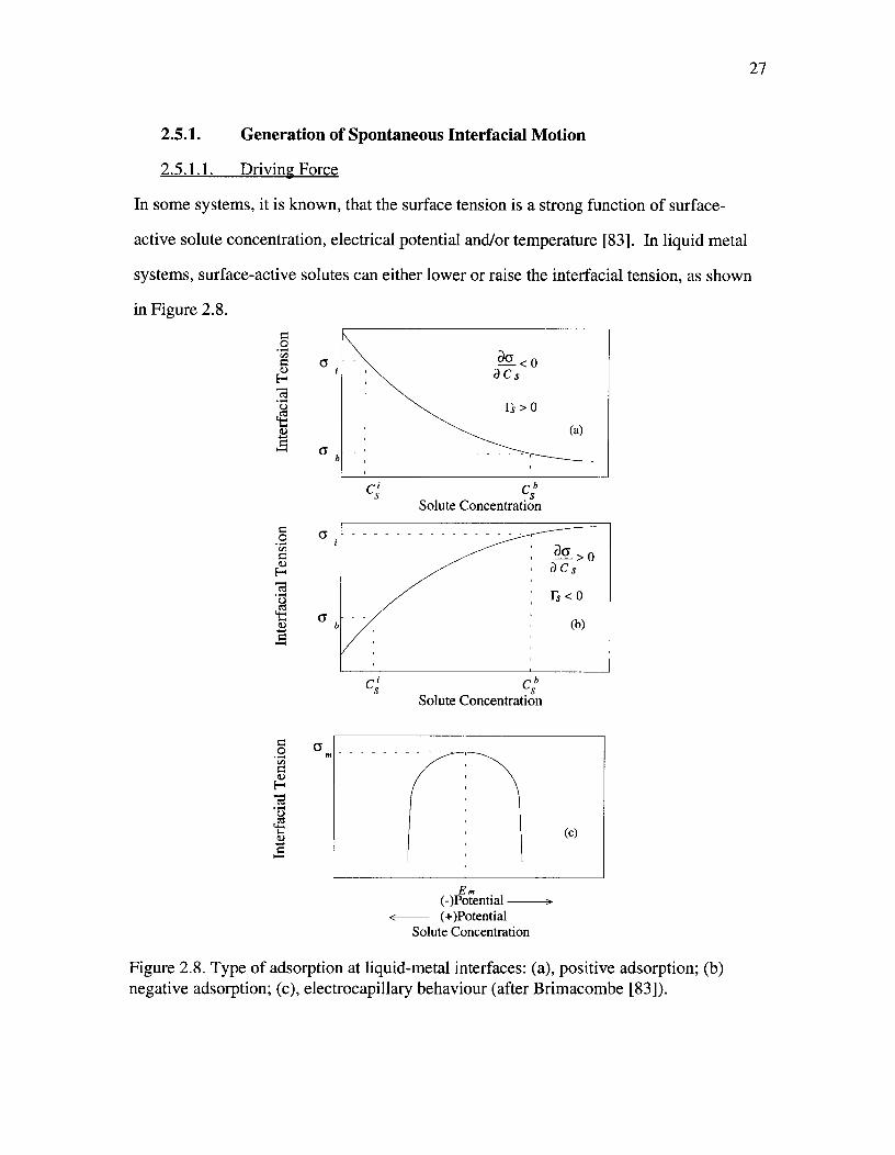
a

CsbSolute Concentration

cs^Csb

Solute Concentration

27

2.5.1.^Generation of Spontaneous Interfacial Motion

2.5.1.1.^Driving Force

In some systems, it is known, that the surface tension is a strong function of surface-

active solute concentration, electrical potential and/or temperature [83]. In liquid metal

systems, surface-active solutes can either lower or raise the interfacial tension, as shown

in Figure 2.8.

Em(-)Potential(+)Potential

Solute Concentration

Figure 2.8. Type of adsorption at liquid-metal interfaces: (a), positive adsorption; (b)negative adsorption; (c), electrocapillary behaviour (after Brimacombe [83]).

0_160.12 020 0.3fi 0.38 0.40

[0] ( w 1 5)

-0-- 1300•C

1230°C

115 0°C

•^1^f^I X

0_04 0.08

28

The dependence of surface tension on the solute concentration is described by Equation

(2.47), which is obtained from the Gibbs adsorption equation [83,86].

(a:5^RT= —Fs

Csacs.lp(2.47)

When two reacting phases are brought into contact, concentration gradients of surface-

active solutes, along their interface, are established. Resulting interfacial tension

gradients may cause the interface to move toward the region of high interfacial tension.

In the case of oxygen and sulphur in copper, it is clear that positive adsorption is

expected, as shown in Figures 2.9 and 2.10.

1300

-E 1200

1 1 0 0

0(I)z 1 000

4-

< 900

(f)

800

Figure 2.9. Effect of oxygen on the surface tension of liquid copper, (after Monma [87]).

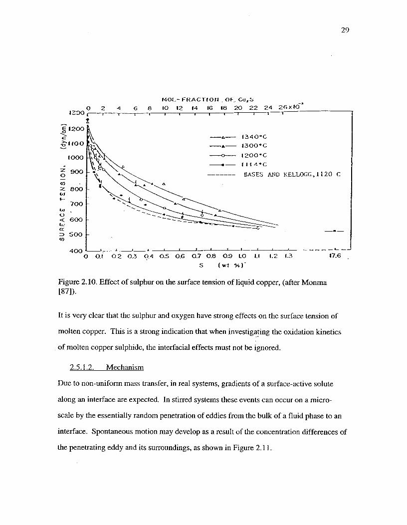
1Z.'90 ^

1200

4000 OA a2 0_3 0.4 05 0.6 02 0.8 OS 10

S^(wt 94.)-

1.3 17.61.2

1000

900;)

800

700

< 600

500(i)

A--- 1340°C

A --- 1300°C

^ 1200°C

1114•C

^ BASES AND KELLOGG,1120 C

1•101.- FRACTIOt4 . OF C-u,S

0 2 4^6 8 10 t2 14 16 18 20 22 24 26 x10

Figure 2.10. Effect of sulphur on the surface tension of liquid copper, (after Monma[87]).

It is very clear that the sulphur and oxygen have strong effects on the surface tension of

molten copper. This is a strong indication that when investigating the oxidation kinetics

of molten copper sulphide, the interfacial effects must not be ignored.

2.5.1.2.^Mechanism

Due to non-uniform mass transfer, in real systems, gradients of a surface-active solute

along an interface are expected. In stirred systems these events can occur on a micro-

scale by the essentially random penetration of eddies from the bulk of a fluid phase to an

interface. Spontaneous motion may develop as a result of the concentration differences of

the penetrating eddy and its surroundings, as shown in Figure 2.11.

29

30

Figure 2.11. Interfacial motion generated on micro-scale due to eddy penetration (afterBrimacombe [83]).

Also macro-scale non-uniform mass transfer of surface-active solute can generate

interfacial turbulence at the mass transfer interface. A hypothetical example of macro-

scale interfacial motion is the case of a solid Cu2S piece partially immersed in molten

copper, as shown in Figure 2.12. In this case, surface motion away from the solid Cu2S

is spontaneously generated. The experiments of Barton and Brimacombe indicated that

interfacial turbulence is generated during the dissolution of solid Cu2S in molten copper

[85].

Figure 2.12. Interfacial motion generated on macro-scale by presence of partiallyimmersed piece of Cu2S in molten copper.

31

As show in Figure 2.13, the effect of oxygen is expected to be similar to that of sulphur.

The experiments of Barton and Brimacombe also indicated that interfacial turbulence can

enhance the liquid phase mass transfer coefficient by at least one order of magnitude

during the absorption of oxygen by liquid copper [56]. In those experiments Ar-02 gas

mixtures were top blown onto molten copper baths. Measurements of surface velocity

and of oxygen concentration in the bath were conducted to determine the effect of surface

tension-driven flows on the kinetics of oxygen absorption by liquid copper. A copper

oxide patch was observed beneath the oxygen lance, and the surface spreads rapidly

outward as shown in Figure 2.13. Spreading of the copper surface in the presence of

copper oxide can be described by the initial spreading coefficient, as follow:

S^ Cu - (a oxide ± a oxidelCu)

02

V

Oxygen lance

(2.48)

Copper oxide patch

Oxide

6 Cu^ 6

^ CuOxide/Cu

Liquid Copper

Figure 2.13. Mechanism of copper oxide patch spreading on the liquid copper surface,(surface spreads if act, cFOxide ± CulOxtcle)•

Having reviewed the practical implications of the effects of oxygen and sulphur on the

surface tension of liquid copper, separately, it becomes very clear that their simultaneous

effect is of a very similar nature. Thus, when investigating the oxidation kinetics of

molten copper sulphide, the effect of surface-tension driven flows must be considered.

3. Objectives and Scope

The understanding of the oxidation kinetics of molten copper sulphide is highly important

to the overall understanding of copper converting. The high oxygen utilization of the

copper converter and the findings of earlier studies indicate that the rate controlling

mechanism of the oxidation reaction of molten copper sulphide is gas phase mass

transfer. There are, however, fundamental discrepancies with respect to the chemistry of

the copper-making stage. Earlier studies indicated that the oxidation of molten copper

sulphide takes place in two stages. The measurements of Rottmann and Wuth [71]

indicated that the ratio of the moles of reacted oxygen to the moles of evolved sulphur

dioxide are greater than unity during the primary stage and less than unity (approximately

0.9) during the secondary stage. Therefore, it is clear that neither Reaction (2.4) nor

Reaction (2.5) can be the reactions during the primary stage. According to the

stoichiometry of Reaction (2.2), the ratio of oxygen to sulphur dioxide is 3/2. This may

suggest that Reaction (2.2) is the primary reaction; however; the thermodynamics of this

system indicates that the formation of Cu20 is not possible before the total oxidation of

Cu2S. Furthermore, the formation of solid Cu20 results in surface blockage and likely

cessation of the oxidation reaction. Therefore Reaction (2.2) is not the secondary copper-

making reaction, as claimed by all of the investigators. It also is clear that treating this

system as an aggregate of neutral compounds results in a fundamental dilemma in

characterizing the form of the dissolved oxygen5: it is well known that sulphide melts are

ionic in nature [24-25,115]. Therefore, in order to correctly deduce the chemical

reactions that take place during the copper-making stage, the electrochemical treatment of

this system must be adopted rather than the conventional (neutral compounds) treatment

adopted by previous investigators.

32

5Since the ratio of the moles of reacted 02 to the moles of evolved SO2 is greater than one, someof the oxygen must dissolve in the melt.

33

Although all of the previous investigators have concluded that the rate controlling

mechanism of the oxidation reaction of molten copper sulphide is gas phase mass

transfer, Jalkanen [57] has suggested that the rate of chemical reaction may be rate

limiting as well. None of the experimental studies provided any results of the reaction

gas flow rate effect on the reaction rates. Perhaps this has not been possible in

experiments involving small bath size (3-7 grams [57]) and in the case of diffusion testes

(0.1-0.15 grams [27]). As explained in Section 2.4, in studying the kinetics of gas-liquid

reactions, it is vital that the effect of reaction gas flow rate be determined.

Earlier studies revealed that the effect of interfacial phenomena in copper baths must be

considered when investigating gas-liquid or solid-liquid reaction kinetics. It has been

established that surface tension-driven flows have a profound effect on the kinetics of

oxygen absorption by molten copper. The effect of interfacial phenomena on the

oxidation kinetics of liquid mattes has not been investigated yet. In the light of this

discussion, the objectives of the present work can be outlined as follows:

1. To elucidate further the rate controlling mechanism of the oxidation reaction

of molten copper sulphide.

2. To investigate the role of spontaneous interfacial motion in the oxidation

reaction of molten copper sulphide.

3. To formulate a mathematical model that can provide the fundamental evidence

in support of the experimental findings.

4. To extend the understanding of the oxidation kinetics of molten copper

sulphide to the copper-making stage in the Peirce-Smith converter.

34

3.1. Experimental Objectives

In order to determine the rate controlling mechanism of the oxidation reaction of molten

copper sulphide, the following experimental objectives were pursued:

1. A series of laboratory tests was conducted to determine the rates of reactions

of molten copper sulphide baths.

2. With the reaction gas composition, the melt volume, and the reaction

temperature fixed, a series of tests was carried out for a gas flow rate range of

1-4 1/min.

3. Fixing all other variables, a series of tests was conducted for a reaction gas

composition in the range of 20-80% 02.

4. Similarly with respect to bath temperature, reaction rates at 1200-1300 °C

were determined.

5. To investigate the role of liquid phase mass transfer resistance in the oxidation

kinetics, an artificially invoked mixing test was conducted in which the

bubbling of argon gas in the bath during oxidation was adopted.

6. In order to determine the effect of surface tension-driven flows on the reaction

kinetics, photography and direct observations of the melt surface were carried

out.

7. Microscopic examinations of frozen melt samples, at pre-defined reaction

conditions, were undertaken to aid in the analysis of the reaction rate results.

35

3.2. Theoretical Objectives

In order to confirm the findings of this work, a mathematical model was formulated and

validated against the experimental results. Based exclusively on gas phase mass transfer

and the electrochemical behaviour of the melt, the model was constructed to achieve the

following objectives:

1. To predict, within an acceptable degree of error, the measured bath sulphur

and oxygen molar contents for the two stages and their time durations.

2. To predict, within a reasonable margin of error, the molar reaction rates of the

sulphur and oxygen as functions of reaction gas flow rate, reaction gas

composition and bath temperature.

Based on the model predictions, the reason for the existence of two stages rather than one

was determined, and the rate controlling mechanism of the oxidation reaction of molten

copper sulphide was confirmed. The electrochemical reactions that take place during the

two stages were inferred.

4. Experimental

4.1. Experimental Apparatus

In order to achieve the experimental objectives, the experimental equipment was designed

and built for use in all of the laboratory tests. The equipment consisted of: a reactor, gas

drying and control system, gas analysis system, gravimetric measurement system

equipped with a data acquisition system, and the melt surface photography system.

4.1.1.^Reactor

The reactor, shown in Figure 4.1, consisted of a vertical tube resistance furnace, with a

reaction tube, heating elements and layers of insulation contained in a steel frame. In the

core of the reactor, an alumina 6 reaction tube, with dimensions of 57 mm inside diameter,

64 mm outside diameter and 762 mm length, was located. Water-cooled brass couplings

were used for the support and mounting of the reaction tube to the steel frame. Vacuum

greased fluorocarbon 0-rings were used to seal the reaction tube to the brass couplings 7 .

Insulating alumina bricks were used for the inner portion of the insulation, immediate to

the heating elements, and firebricks were used for the outer portion, between the

insulating alumina brick layer and the steel frame8 . Porcelain wool was used to fill the

gaps between the bricks.

Four 2-shank KANTHAL SUPER heating elements were carefully mounted around the

reaction tube and connected in series. The heating elements were connected to a 5 kW

power-supply9 . Using this set-up, approximately 40 mm of ±0 °C hot zone was obtained.

699.7% recrystallized alumina was used in all of the reactor components that are within andincluding the reaction tube.7To prevent the corrosion of the inside surface of the brass coupling, due to the long termexposure to SO2, the inside surface of the brass coupling was vacuum greased.8Reactor insulating materials properties are provided in Appendix A.9For more details about the electrical circuit of the power-supply, refer to Figure A.1 inAppendix A.

36

37

Figure 4.1. Cross-sectional view of the reactor.

38

To maintain constant electrical conductivity of the electrical connectors of the heating

elements, two electric fans were used to cool the exposed portions of the heating

elements.

Approximately 200-gram samples of molten copper sulphide were held in cylindrical, flat

bottom, alumina crucibles of approximately 44 mm inside diameter, 50 mm outside

diameter and 75 mm height. The crucible supporting post, shown in Figure 4.2, consisted

of a closed end alumina tube (6 mm I.D., 10 mm O.D. and 450 mm long) attached to an

alumina disc (40 mm in Dia and 3 mm thick), with high temperature ceramic cement.

Figure 4.2. Sectional view of the bottom of the reaction tube, including the cruciblesupporting system. Note that the scale is offset to show the rubber diaphragm sealingarrangement.

A thin sheet of porcelain wool was used as an insulator between the bottom of the

crucible and the alumina disci°.

The bottom of the reaction tube consisted of a brass plate with a port for the crucible

supporting post. For safety reasons and for the purpose of analyzing the off-gas, the

system had to be very tightly sealed. A neoprene diaphragm arrangement was used to

seal the bottom of the reactor, as shown in Figure 4.2.

The top of the reaction tube, shown in Figure 4.3, consisted of ports for the lance, the

auxiliary tube and the thermocouple sheet, the off-gas outlet pipe, and two viewing ports.

The alumina tubes were fitted and sealed in the ports by 0-rings. Due to the

condensation of water vapor on the lower surface of the viewing port, the ability to clean

the surface easily without allowing a large amount of gas to escape, required the viewing

ports to be equipped with shutters, as shown in Figure 4.3. The off-gas outlet pipe,

permanently attached to the top of the reaction tube, consisted of a copper pipe of 6 mm

inside diameter, 8 mm outside diameter, and 400 mm length.

39

10Due to the release of the heat of fusion of the solidifying bath, during the withdrawal of thecrucible, the alumina disc was susceptible to cracking as a result of its low thermal shockresistance.

I1^

Socket-HeadSet Screw

Viewing Port Shutter/ ,^Quartz Disc(^IFluorocarbon

0-Ring

Plan View

Polypropylene 0-Ring

I^I103 mm

40

Top View

Off-Gas Pipe

Viewing,Photographingand Sampling

Port

Auxiliary TubePort

Brass Plate

ThermocouplePort

LancePort

Figure 4.3. Schematic diagram of the top of the reaction tube.

SO 2 Supply

Plexiglas Columns60 mm ID, 70 mm OD,

300 mm H

-

-

35\ To Lance

To AuxiliaryTube

OptionalRotameter

Calibration andExhaust Gas Line

Option

Rotameters

gi9 Pressure^ Gauge

0

r'

MercuryManometer

Ar/O2Supply

41

4.1.2.^Gas Drying And Control System

To control the gas flow rate and composition, and to reduce its moisture contentil, the gas

control and drying system, shown in Figure 4.4, consisted of gas drying columns,

rotameters, pressure gauge, mercury manometer and thermometer. Polyflow lines were

used to connect the components of the gas control and drying system.

Silica Gel^02 Supply Calcium SulphateFigure 4.4. Schematic diagram of the gas train (not to scale).

4.1.3.^Gas Analysis System

Manual measurements of the reaction rates were conducted by the use of an SO2 gas

absorber and a soap bubble meter. Due to its simplicity, the manual measurement system

was found to be very reliable and more accurate than gravimetric measurement.

However, gravimetric measurement was found to provide a general support to the manual

11Water vapor, in the reaction gas, condenses on the inner surface of the quartz discs andprevents surface observations.

42

measurement. The gas analysis consisted of the determination of the amount of sulphur

removed from the bath by the use of the SO2 absorber and of the amount of unreacted

oxygen using a soap bubble meter.

4.1.3.1.^SO2 Absorber

The SO2 gas absorber consisted of approximately 3 liters of 5 % H202 solution

vigorously mixed in a Plexiglas column, as shown in Figure 4.5.

Figure 4.5. Schematic diagram of the off-gas analysis system, not including the soapbubble meter.

43

In order to reduce the temperature of the off-gas before introducing it to the absorber, it

was passed through a 300 mm long water-cooled copper jacket, as shown in Figure 4.5.

To determine the amount of SO2 absorbed, a sampling port with a rubber stopper was

constructed in the master rubber stopper of the absorber. Using a 5-ml pipet, samples

were extracted through the sampling port, at specific intervals of reaction time. During

the time of the final gas flow rate measurement, using the soap bubble meter, the

sampling port was sealed to prevent escape of the final off-gas. Due to the high aspect

ratio of the absorber, vigorous mixing of the solution had to be ensured for the extraction

of representative samples. In order to achieve simultaneous mixing and sealing of the

absorber, the stirrer shaft had to be sealed to the rubber stopper port as shown in Figure

4.6.

Figure 4.6. Schematic diagram of the absorber rubber stopper (not to scale).

Once the bubbles come in contact with the hydrogen peroxide solution, the SO2 is

absorbed from the bulk gas according to the following reaction:

[H202] + (SO2) = [1-12SO41^ (4.1)

44

To ensure high SO2 absorption efficiency, vigorous mixing, a high aspect ratio of 6 and a

sufficient amount of the 5% H202 solution were adopted. It is well known that the rate

of Reaction (4.1) is very fast [44]. Hence, in such a system, the rate must be bubble

volume limited i.e. the smaller the average bubble size, the higher is the absorption

efficiency. Vigorous mixing of the solution and the introduction of the gas at the wall of

the absorber caused the gas bubbles to disintegrate to a small size and to be retained in

the region of the propeller, as shown in Figures 4.5 and 4.8, thereby increasing their

retention time and ensuring complete absorption of the SO2. The high aspect ratio was

also important in achieving the high absorption efficiency.

The total possible amount of SO2 that might be evolved from the oxidation of 200 grams

of Cu2S is approximately 1.257 moles. Therefore, according to Reaction (4.1), the

corresponding amount of H202 required is also 1.257 moles. However, to ensure

complete SO2 absorption, 3 liters of 5% H202 solution system was utilized i.e.

approximately 4.4 moles of H202.

To determine the amount of SO2 absorbed, the samples were titrated with 0.1 N NaOH

standard solution, according to Reaction (4.2). Thus the moles of SO2 were calculated,

accordingly, from Equation (4.3).

[H2SO41+ 2[Na011]=[Na2SO4]+2((H20))

ATS02

V= NaOHN NaOH v'' 217,

To test the absorber performance, an Ar-S02 gas mixture was admitted at a constant flow

rate and composition for approximately 60 minutes. Samples were obtained at pre-

defined intervals of time and the amount of SO2 absorbed was determined by acid-base

titration. The measured absorbed SO2 was found to be in agreement with the admitted

amount as shown by Figure 4.7.

(4.2)

(4.3)

45

Figure 4.7. Plot of the amount of SO2 absorbed as a function of time for a test of 2 1/minof 13 % SO2 and 87% Ar at 23 °C.

The absorber performance was also tested by admitting approximately 260 ml/min of

pure SO2 The gas flow rate from the absorber was found to be approximately 0 ml/min.

The gas bubbles were observed to diminish in size as they traveled upward to the solution

surface, as shown in Figure 4.9.

11111111111114Figure 4.8. Photograph of the SO2 absorber with a gas flow rate of 21/min, 13 % SO2and 87 % Ar. Note the vigorous mixing attained by the design of the absorber.

46

Figure 4.9. Photograph of the SO2 absorber with a gas flow rate of 260 ml/min pure SO2.

To determine the validity of the kinetic measurements, the following calibration

procedure was performed both before and after each run:

1. An Ar-S02 gas mixture with a gas flow rate and composition close to that of

the expected off-gas (assuming 100 % oxygen utilization), was admitted for a

period of 10 min.

47

2. A sample was obtained and the amount of SO2 absorbed was determined by

titration and compared to the admitted amount.

3. The final off-gas flow rate was measured by the soap bubble meter and

compared to the above results.

4. The final off-gas was tested by smell to detect any residual SO2.

5. If the above results were found to be consistent and the absorber efficiency

was found to be very close to 100 %, the results of the respective run were

accepted12.

4.1.3.2. Final Off-Gas Flow Rate Measurement

In order to determine the final off-gas flow rate accurately, an appropriate size of the soap

bubble meter was selected, for the given reaction conditions. Using a stop watch, the

time that a soap bubble takes to travel over a certain height of the graduated cylinder was

determined. To determine the gas flow rate, the volume was divided by the measured

time.

48

Graduated Glass Tube

Digital Piercing Thermometer ^

Rubber Bulb For

Injecting Soap Bubble;—\

Final Off-Gas From SulphurDioxide Absorber

Copper Pipe (heat exchanger)6 4 mm inside diameter,7.9 mm outside diameterand 1 m long

Rubber Hose

Retort Stand

Figure 4.10. Schematic diagram of the soap bubble meter.

12Due to the low percentage of rejection, approximately 3% for the entire program, the SO2absorber was considered to be very effective.

Fixed EndUpper Strain

Gauges

To Data AcquisitionSystem

/1

//Pre-MarkedFree End

Daytronic StrainGauge Signal

ConditionerModel 601B

Crucible Supporting Post

Lower StrainGauges

Fixed EndBracket

Steel Bar

49

To ensure accurate measurements, graduated tubes that resulted in relatively low bubble

velocities, of approximately 20-50 mm/sec, were used. Depending on the expected final

off-gas flow rate, the size of the soap bubble meter was selected. For final off-gas flow

rates of 2 1/min, a 500-ml graduated tube was selected and for the measurement of final

off-gas flow rates of < 2 1/min, a 250-ml graduated tube was used.

4.1.4.^Gravimetric Measurement System

In order to obtain automatic measurement of the bath weight, a gravimetric measurement

system, consisting of weighing and recording devices, was custom assembled from a load

cell and a data acquisition system.

The load cell consisted of a cantilever beam that was made of a 3x19x120 mm steel bar,

four temperature compensated strain gauges and strain gauge signal conditioner,

assembled as shown below.

Figure 4.11. Schematic diagram of the load cell".

13For more details about the electric circuit and the components of the load cell, refer toAppendix A.

The data acquisition system was comprised of a 286 IBM PC equipped with CIO-ADO8

data acquisition board with a total of 32 channels, data acquisition program and a

spreadsheet program.

The crucible supporting post was placed on the pre-marked free end of the cantilever

beam, as shown in Figure 4.11. The fixed end of the cantilever beam was attached to the

support frame by means of the fixed end brackets such that the beam could swing to the

side to permit removal of the crucible at the end of a run.

As mentioned earlier, the gravimetric measurement was found to be less reliable than the

manual gas analysis to characterize the reaction rate. This is due to the fact that when

placing the alumina post on the load cell, it was difficult to determine whether it was

completely free 14 . It was only after 10 minutes of the reaction time that the visual display

of the gravimetric measurement on the PC screen, indicated if the measurement was

successful. The gravimetric measurement, therefore, was used only as a general check on

the validity of the results of the manual gas analysis. The rate of bath weight change was

exclusively used in comparing the gas analysis results to the gravimetric measurement

results. The overall rate of bath weight change was obtained by performing linear

regression of the bath weight with time. Statistically, the validity of this regression was

dependent on the number of data collected over relatively long periods of time. This was

often possible during the secondary stage only. In most of the runs, during the primary

stage, it was not possible to obtain reliable results.

14Success of the measurements was contingent upon the crucible being concentric with respect tothe reaction tube. On occasion, however this was difficult to accomplish because of the nature ofthe crucible supporting post. Due to manufacturing defects, the alumina tubes, used in makingthe crucible supporting posts were often warped at the bottom (in the vicinity of the bottom ofthe reaction tube). Because the gravimetric measurement system was added to the apparatus at alater stage of the experimental program, it was not possible to modify some key components ofthe apparatus to eliminate all of the problems associated with the gravimetric measurementsystem. For a newly designed apparatus, however, the elimination of these problems can beachieved.

50

Line

o Initial

A Final

Standard weights were used in the calibration of the load cell before and after each run.

An average equation for the relationship of the weight and the load cell reading was

obtained to convert the load cell response to weight measurement. As the relationship

between the weight and load cell reading is linear, as shown by Figure 4.12, a typical

equation for the best line can be calculated as follows:

W= 87+82R,

0^

100^

200^300^

400^

500

Weight (grams)

Figure 4.12. Load cell calibration plot obtained with standard weights.

The load cell response, during the reaction time, was recorded by the data acquisition

system and stored in a spreadsheet. The millivolt readings were converted by the

calibration equation of the respective run.

51

(4.4)

52

Constant load cell reading for a period of time or permanently until the end of a run was

observed to take place during some experiments. This indicated that due to some

mechanical interference in the weighing system, the load cell was not measuring the full

weight. Then depending on how long this interference took place, the measurement was

either completely discarded or the straight line segments were used to calculate an

average value for the rate of weight change. Due to the stabilization process that the

system undergoes, as a result of the internal pressure change '5 at the beginning of the

reaction, the measurements that were obtained during the first minute were discarded.

For the secondary stage, reading for at least 10 minutes was taken as a valid

measurement. To determine the validity of the measurement and its time domain the

sample weight was plotted against time and examined visually. Using the least squares

method [105], linear equations for weight as a function of time, were calculated for the

linear portions of the measurement. To determine the rate of weight change, the

equations were differentiated with respect to time as follows:

iil . dW d ,= La+ bt]= b

dt dt

4.1.5.^Optical Photography System

In optimizing the furnace parameters, the volume of the reaction tube was kept to a

minimum in order to minimize the gas measurement time lag. This resulted in relatively

small view ports, of approximately 20 mm in diameter. In order to photograph the melt

surface, of approximately 44 mm, the need to design a specific optical system was

inevitable. The variable focal length optical system consisted of a 450 mirror to reflect

the image horizontally, a focusing macro-lens and a magnifying eyepiece, as shown in

15As a result of passing the off-gas through the SO2 absorber, the pressure head of the solution ofthe absorber increased the internal pressure of the reactor in a non-steady state manner at thebeginning of the reaction.

(4.5)

>^

>^

\TA,

Figure 4.13. This system of lenses was installed on a 35 mm camera with the use of a

bellows.

53

250 mm1

70 mm 35 mm1^1#

35 mm Film

45 ° MirrorFocal Point

irla (4111Focusing

Macro-Lens1:2/50

Magnifying LensPlan Corrected

Eyepiece

Alumina Reaction Tube400MM

Alumina Crucible

Melt Surface

# Variable dimensions

•01d,

^ 44 mm —IFigure 4.13. Schematic diagram of the optical system used in the photography of the meltsurface. The lenses were mounted and enclosed within a system of bellows.

4.2. Material

4.2.1.^Copper Sulphide

4.2.1.1.^Supplied Copper Sulphide

Approximately 99.5% copper sulphide, monoclinic Cu2S (-200 mesh) supplied and

certified by Cerac Inc. was used for all of the runs except for the first 5 runs. The

chemical analysis given in Table 4.1 indicated that the impurities are negligible in

quantity.

Table 4.1. Trace analysis (wt%) of supplied copper sulphide.

Ag <0.01

Al <0.01

Ca < 0.01

Cr <0.01

Fe <0.01

Mg <0.01

Mn <0.01

Ni <0.01

Pb <0.01

Si <0.01

Sn <0.01

Ti <0.01

Zr <0.01

4.2.1.2.^Prepared Copper Sulphide

For the preliminary runs (the first 5 runs), prepared Cu2S was made of 99.9 % pure

copper powder and laboratory reagent grade elemental sulphur. Approximately 1590

grams of copper were well mixed with approximately 410 grams of sulphur16 in a

graphite-clay crucible. The crucible was then placed in a larger graphite crucible, to

161n order to compensate for the loss of sulphur during the Cu2S reaction, approximately 2 %excess sulphur was used.

54

55

avoid damaging the furnace material in case of spillage. The crucible was then covered

with a graphite lid and placed in a preheated muffle furnace, at approximately 400°C, for

approximately 3.5 hours. To minimize sulphur evaporation prior to its reaction with

copper, the reaction was allowed to take place at a temperature of 50 °C below the boiling

point of elemental sulphur, according to Reaction (4.6). To prevent excessive reaction of

oxygen with the copper sulphide, argon gas at a flow rate of approximately 200 ml/min

was passed through the furnace.

2(C0+ ((s)) = (Cu2S)^ (4.6)

In order to homogenize the copper sulphide by melting according to Reaction (4.7), the

crucible was then placed in another preheated muffle furnace, at approximately 1200 °C,

with argon atmosphere, for approximately thirty minutes. The crucible was then carefully

removed from the furnace and placed on a steel plate, to slow cool. The copper sulphide

ingot then was removed from the crucible and crushed into small granules, for use.

However, due to the difficulties in repreparing the same composition and the cost of

chemical analysis, the use of prepared copper sulphide was terminated.

(Cu2S) = ((Cu2S))^ (4.7)

4.2.2.^Gases

Ar-02 mixtures were used for most of the runs, except for a run to investigate the effect

of reaction gas carrier type, where a N2-02 mixture was utilized. Ar-S02 gas mixtures

were employed for the calibration of the gas analysis system. The impurity specifications

of these gases are as given in Table 4.2. In order to reduce the moisture content of the

gases, they were passed through silica gel and CaSO4 columns before being admitted into

the reaction tube, as shown in Figure 4.4.

56

Table 4.2. Imnuritv s ecifications of gases in porn.

Gas Minimum

Purity

N2 02 H20 CO2 THC Kr Ar

07 (U H P) 99.995% <40 <5 <1 <1 <15 <15

N7 (U H P) 99.999% <5 <5 <1 <1 <25

Ar (Pre-purified) 99.998% <3 <5

SO2 (Anhydrous) 99.98%

4.2.3.^Hydrogen Peroxide Solution

To prepare approximately 5% H202 solution for the absorption of SO2, approximately

2500 ml of de-ionized water was added to 500 ml of 30% H202 solution, for which the

chemical analysis is given in the Table 4.3. Due to their insignificant concentrations in

the supplied hydrogen peroxide solution, the impurities were ignored in the determination

of the amount of SO2 absorbed.

Table 4.3. Maximum limits of impurities for the 29.0-32.0 % hydrogen peroxide solutionsuonlied by BDH .

Impurity Maximum Concentration

Residue after evaporation 0.002 %

Titratable acid 0.006 meq/g

Chloride (Cl) 3 Ppm

Nitrate (NO3) 2 ppm

Phosphate (PO4) 2 ppm

Sulphate (SO4) 5 Ppm

Ammonium (NH4) 5 PPIn

Heavy metals (Pb) 1 ppm

Iron (Fe) 0.5 ppm

57

4.2.4. Titration Reagents

Approximately 0.1 N NaOH standard solution was used in the acid-base titration of the

samples obtained from the gas absorber. The NaOH standard solution was prepared by

dissolving pre-weighed amounts of reagent grade solid sodium hydroxide in de-ionized

water and storing it in plastic bottles. The NaOH solution was then standardized by

potassium hydrogen phthalate (KHC811404) [106] and labeled for use. The chemical

analysis given in Table 4.4 indicated that after standardizing the prepared solution, the

effect of impurities in the solid hydroxide can be ignored.

Table 4.4. Maximum limits of impurities for the 98.0 % sodium hydroxide pellets(supplied by BDH).

Impurity Maximum Concentration (%)

Water insoluble matter 0.01

Carbonate (Na7CO3) 1.0

Chloride (Cl) 0.005

Phosphate (PO4) 0.001

Silicate (Si07) 0.01

Sulphate (SO4) 0.005

Aluminum (Al) 0.001

Calcium (Ca) 0.002

Copper (Cu) 0.0005

Iron (Fe) 0.0005

Lead (Pb) 0.0005

Nickel (Ni) 0.0005

Potassium (K) 0.05

Nitrogen Compounds (N) 0.0005

Approximately 0.1 % phenolphthalein was used as an indicator for the acid-base titration.

The indicator was prepared by dissolving the solid in 80 % ethyl alcohol [106].

58

All glassware was cleaned with the use of laboratory glassware cleaning solution and

soap. The cleaning solution was prepared by mixing 10-15 grams of potassium

dichromate (K2Cr207) with about 15 ml water, in a 500 ml heat resistant conical flask.

Enough concentrated sulphuric acid was added slowly, until all of the forming solid was

dissolved. The solution was discarded when it acquired a green color [108].

4.3. Experimental Procedure

4.3.1.^Oxidation Rate Measurement

To measure the rate of oxidation of the molten copper sulphide bath, the following steps

were followed :

1. Before each run, a complete leak test was performed on all of the couplings,

polyflow fittings and valves. Leak tests were performed by pressurizing the

system and testing for leaks by the use of bubbling soap. The gas supplies

were also checked to ensure sufficient supply for the run.

2. Approximately 200 grams of the solid Cu2S were weighed in an alumina

crucible. The crucible was then carefully placed at the bottom of the reaction

tube, on the alumina supporting post. The bottom of the post was placed on a

laboratory jack, which was used to push up the post until the crucible was

located at a pre-defined position, in the hot zone. To avoid thermal shock, the

crucible was pushed at a rate of approximately 10 mm/min. During the

preheating and melting of the sulphide sample, approximately 50 ml/min of

argon was introduced through the preheating tube.

3. During the melting of the sulphide sample, the load cell and gas absorber were

calibrated, and the data acquisition system was activated.

4. After the calibration of the load cell, the jack was removed and the alumina

post was carefully placed on the marked end of the load cell as shown in

Figures 4.1 and 4.11.

5. After ensuring that the sample was completely molten, by surface observation

and from the temperature, the reaction gas flow rate and composition were

adjusted to the desired levels, and the thermocouple was lifted from the bath

to the vicinity of the lance nozzle17. The reaction gas was then admitted to the

reaction tube, through the lance, and the data collection proceeded

immediately.

6. The data collection was done via two independent sources: the gas analysis for

SO2 and 02, and the gravimetric measurement of the bath weight.

7. Due to the corrosive nature of copper oxide, the reaction was terminated just

before Cu20 began to form. As the oxidation reaction of molten copper

sulphide ended, the spontaneous motion of the surface was observed to cease.

8. The final calibration of the gas absorber and the load cell were carried out.

9. The temperature of the system was recorded throughout the run by the data

acquisition system and stored in a spread sheet. Using the mercury

manometer, the pressure of the system was monitored periodically throughout

the run and an average value was recorded.

10. The load cell was released and swung to the side for removal of the crucible.

11.The crucible supporting post was then placed on the laboratory jack. The jack

was then lowered at the rate of approximately 10 mm/min. This was

17Due to the intensity of the oxidation reaction, corrosion of the thermocouple sheath and theplatinum thermocouple was found to take place if the same thermocouple sheath was used inmore than one run, with its tip immersed in the melt.

59

important to avoid the rapid release of the heat of fusion, which started at

approximately mid-distance from the bottom of the reaction tube.

12.The crucible was removed after it reached the bottom of the reaction tube.

Once the temperature of the crucible reached room temperature, its weight

was determined and recorded.

13. All of the glassware was washed and prepared for the next run.

4.3.1.1.^Gas Analysis

In order to determine the amount of sulphur removed from the bath as a function of time,

samples were extracted from the gas absorber, at pre-defined time intervals, with a 5-ml

pipet. The samples were stored in pre-labeled 250-rn1 conical flasks, until the end of the

run. Due to the exothermic nature of the absorption reaction, the temperature of the

solution was observed to increase at a constant rate. This was used as another indicator

of the efficiency of the absorber in a particular run. For each sample obtained, the

temperature of the absorption solution was recorded. The amount of sulphur dioxide

absorbed was determined by the acid-base titration of the individual samples, using 0.1 N

NaOH standard solution [107]. Since the molar ratio of sulphur to sulphur dioxide is

unity, the number of moles of sulphur removed from the bath is the same as the moles of

sulphur dioxide absorbed.

To determine the amount of unreacted oxygen in the off-gas, the soap bubble meter was

used to measure the off-gas flow rate. For each absorber sample obtained, at least four

volumetric flow rate measurements were made. Due to the increase of the temperature of

the absorption solution, the temperature of the gas was expected to deviate from room

temperature, as it left the absorber. In order to avoid temperature effects, the temperature

of the gas inside the rubber hose, leading to the soap bubble meter, was recorded for each

set of measurements.

60

61

4.3.1.2.^Gravimetric Measurement

This measurement was used to verify and support the gas analysis measurement. The

reaction system weight was performed automatically, using the data acquisition system.

The numerical load cell response was converted to weight using the calibration equation.

4.3.2.^Microscopic Examination of Frozen Melt Samples

For further validation of the kinetic measurements, melt samples of known reaction were

obtained and microscopically examined. U-shaped quartz tubes with an approximate

inside diameter of 5 mm were used to obtain approximately 4- 7-gram samples at specific

intervals of reaction time. To minimize post sampling reaction, the samples were

immediately quenched in an ice bath. The samples were sectioned, hot-mounted and

polished using 5 gm and 1 gm alumina polishing powder. The samples were then

examined with an optical microscope to assess copper droplets, gas bubbles and the

phases present.

4.3.3.^Surface Observation

Surface observations were primarily undertaken to investigate the effect of surface-

tension driven flows on the reaction kinetics. The observations included the qualitative

measurement of surface movement, gas bubbles rising from the melt and surface velocity,

under different reaction conditions. The surface observations also served as an indication

of the state of reaction and its termination. Using a 35-mm camera and the optical system

presented above, some runs were conducted to obtain photographic evidence of the visual

observations. Photographs were taken of the melt surface under specific reaction

conditions.

ReactionChamber

I W(t), T(t)Figure 5.1. Gas flows in the oxidation experiments.

A No2 (t)

Bubble Meterv Tg (t) ^Y

N^ ,(t) T(t)SO2

4 (0Q7.^>

Absorber5%H2 02

Off-Gas

Soap

62

5. Experimental Results and Discussion

5.1. Oxidation Rate Results

5.1.1.^Gas Analysis Data

5.1.1.1.^Sulphur and Sulphur Dioxide Analyses

The gas flows, which were characterized to determine the oxidation kinetics of molten

Cu2S, are shown schematically in Figure 5.1. Typical results of the gas analysis, for each

run, are plotted against time, in Figures 5.2-5.3. Because all of the SO2 is absorbed by

the 11202 solution, the moles of sulphur in the bath, N8 (t), can be calculated from the

moles of SO2, N80 (t), absorbed as follows:

N8(t)=N—N80(t)^ (5.1)

Figure 5.2 reveals that there are two distinct stages, primary and secondary, for the

formation of S02. In order to determine the rates of SO2 formation and the time domains

of the two stages, the following analysis was carried out:

1. The time domains of the two stages were determined, as a first approximation,

by visualization of the SO2 vs. time graphs.

2. Since the time dependence of the two stages appears to be linear, a linear

equation for each stage was calculated, via regression analysis; and the

transition time was calculated by equating the two equations. If the calculated

transition time was found to be within the time domain of the adjacent two

40^5010^20^300

1.6

1.4

1.2

0

0.4

0.2

0.0

o

63

measured points, the equations were accepted. If the calculated transition time

was found to be closer to another measured value, the linear equations were

recalculated, based on the new designated values. This procedure was iterated

until the best agreement between the measured and calculated values was

achieved. Once the equations were accepted, the slopes of the equations were

regarded as the measured SO2 molar rates.

Time (min)

Figure 5.2. Moles of reaction gas and off-gas as a function of time, for the experimentalconditions of: 200 grams of Cu2S, 2 I/min of 35% 02 and 65% Ar, at 1200 °C; ^regression line for the absorbed SO2; 0 measured absorbed SO2; — — — regression linefor the dissolved 02; 0 dissolved oxygen by difference; — - - — reacted oxygen;^ admitted 02.

1600

64

1•11

1400

,R 1200

a 1000

r:4

^

800

0

^

600 o

400

200

0

0^

10^20^30^40^50Time (min)

Figure 5.3. The final volumetric off-gas flow rate as a function of time for theexperimental conditions of : 200 grams of Cu2S, 21/min of 35% 02 and 65% Ar, at 1200°C; ^ measured final flow rate; - -^- reacted oxygen flow rate; — -A- unreactedoxygen flow rate.

Assuming that the reaction takes place uniformly over the melt surface area, the SO2

molar fluxes were calculated by dividing the SO2 molar rates by the crucible cross-

sectional area, as follows:

n so2A

(5.2)

65

5.1.1.2.^Oxygen Analysis

The amount of oxygen dissolved in the bath as a function of time was determined from

the measured SO2 and the final off-gas flow rate measurement by the following

procedure.

The admitted volumetric gas flow rate, Q , was composed of argon QA„ and oxygen,

as follows:

= 0)2 +^ (5.3)

The volumetric off-gas flow rate, Qoiff (t), varies with time, with an unknown quantity of

SO2, Qs02(t), unreacted 02, Qou2(t), and Ar, as described by the following equation.

aff (t) = QAr 0)2 (t) QS02(t)^

(5.4)

After the 502, the volumetric off-gas flow rate, Q.offf(t), also varies with time, with an

unknown quantity of unreacted 02 and Ar, as described by the following equation.

Q(t)=^(t)^ (5.5)

Having defined the volumetric flow rate equations, the calculation of the volumetric flow

rate of unreacted oxygen can be readily carried out. Since the gas temperature was not

constant, this calculation was based on molar flow rates rather than volumetric flow rates.

Assuming that the gas mixture is ideal, the final volumetric gas flow rate can be

converted to molar flow rate as follows18:

N off (t) =^of^Q(t)P

^R1(t)^ (5.6)

Therefore the unreacted molar flow rate of oxygen can be determined from Equation

(5.7).

18Note that the molar flow rate of Ar, N Ar, is calculated from the rotameter reading (volumetricflow rate) which was calibrated at room temperature. There may be a difference between thetemperature of the measurement of the final off-gas flow rate and the rotameter calibrationtemperature.

66

. u^. f^.

N 02(0 = N off (t)— NAr^ (5.7)

The molar flow rate of unreacted oxygen is converted to volumetric flow rate as follows:

. .

N 0,(07;(t) Z2(t)=^

P

(5.8)

A molar balance on the oxygen yields the following.

QL,(t)= Z, - Q1(4), (t)^ (5.9)

To determine the molar rate of reacted oxygen, the volumetric flow rate of oxygen is

converted to molar rate, according to the following equation.

XTro,(t)= QL2 (t)13R7(t)(5.10)

This molar flow rate of reacted oxygen is calculated from the measured final off-gas flow

rate, for specific intervals of reaction time. The integrated measured molar flow rate of

reacted oxygen is described as follows:

0 rNL2(t) = Nii(t1)+ 5 N 02(t1_2)dt

t

(5.11)

To determine the molar flux of reacted oxygen, linear regression was applied to the data

obtained from Equation (5.11). The molar rate of reacted oxygen was found to be

constant throughout the reaction duration, as shown in Figures 5.2-5.3. Hence for

simplicity, the function of time notation, (t), is dropped. The oxygen molar flux was

calculated by dividing the calculated molar flow rate of reacted oxygen by the cross-

sectional area of the crucible ( for notational simplicity, from this point on, the superscript

r is dropped), as follows:

°^N 02n 02 =

A(5.12)

67

Since the oxygen reacted must be removed in the form of SO2 or dissolved in the bath,

the oxygen dissolved in the bath can be determined by a material balance on the oxygen

as follows:

N[0](0= 2[NL2 (t) NS02 (t)]^

(5.13)

Assuming plug flow conditions, the real time in the reaction was calculated by

subtracting the time needed for a given flow rate of gas to travel the distance from the

reaction surface to the gas absorber ( the volume of the off-gas line was approximately 1

liter and the employed range of volumetric flow rate was 1-4 1/min which resulted in a

time lag of 15-60 s).

In order to study the reaction kinetics, the measured sulphur and oxygen contents in the

bath were plotted on graphs such as that of Figure 5.4. Comparing the closeness of the

measured values to the regression lines, the sulphur analysis exhibits less scatter than the

oxygen analysis. From Figure 5.4, the sulphur and oxygen contents in the bath vary

linearly with respect to time. Thus the rate at which the sulphur is removed from the bath

is constant, but different in the two regimes. Similarly, the respective rate of oxygen

dissolution in the bath is also constant over the primary and secondary stages. In trying to

understand the reaction mechanism, the oxygen behaviour is obviously the first clue. As

shown in Figure 5.4, the amount of dissolved oxygen increases linearly to a certain value

at the transition time, and then decreases to a minimum value, at the final reaction time.

1.4

68

' "^"

10^20^30

Time (mm)

0.0 0^

0 40^50

Figure 5.4. The molar sulphur and oxygen contents of the bath as a function of time, forthe experimental conditions of: 200 grams of Cu2S, 2 I/min of 35% 02 and 65% Ar, at1200 °C; ^ regression line for the amount of sulphur in the bath; 0 measured amountof sulphur in the bath; - - - regression line for the amount of dissolved oxygen in thebath; 0 determined amount of dissolved oxygen.

5.1.1.3.^Overall Reaction Rate

Further analysis of the reaction kinetic data can be accomplished by examining the bath

weight change with respect to time. The rate of weight change of the bath, W, can be

related to the rate of sulphur dioxide evolved from the bath, Nso2 , and the rate of oxygen

reacted, NO2, as follows:

69

.^.W = N o2 MO2 — N so2 Ms02 (5.14)

In order to study the oxygen and sulphur behaviour simultaneously, the bath weight was

plotted for each run in graphs typical of that shown in Figure 5.5.

205

155

0

195

Ecl 185

',..4td:i*1-5

- 175cri

gq

165

, . 1 i i^I " "

10^20^30^40^

50

Time (min)

Figure 5.5. Change of bath weight with time for the experimental conditions of: 200grams of Cu2S, 2 I/min of 35% 02 and 65% Ar, at 1200 °C, ^ calculated fromEquations (5.15) and (5.16); 0 calculated from Equation (5.17).

70

The sample weight was calculated by integrating the rate of weight change with respect to

time, as given by Equations (5.15) and (5.16) by using the determined amounts of oxygen

and sulphur as given by Equation (5.17)19.

. P^. P^ (5.15)147gPa (t)= Wga (0) + [No, Mo, —Nso, Mso, l•t

,^0 s^0 s

Ka(t)= Wga(t* ) +[N 0, M0 — N so, M so,]•(t — t*)

Wga(t)= W(0)+[NO2(t)M0, — N.,02(t)M502]

5.1.2.^Gravimetric Measurement Data

(5.16)

(5.17)

The sample weight measurement, determined gravimetrically with the load cell

arrangement, was plotted against time for each successful experiment, an example of

which is shown in Figure 5.6. Applying the least squares method, the rate of weight loss

in the two stages and the reaction transition time were determined. The reaction

transition time is the time at which the rate of sulphur dioxide formation changes. In the

gravimetric measurement, the reaction transition time is the time at which the rate of

weight loss changes.

19Note that Equations (5.15) and (5.16) describe the regression lines obtained from the measuredresults and Equation (5.17) represent the individual measured data points.

220

210

200

g 190 —0 GS^0^Q0 Q)bo

74a° 180 ^'51

ft 170 ^til

1600

150

0_0 g

0 V 011445° t0 (O 0

0 . •of%

r';',^00

•(a 0...• elles

or

90 90

-

140ÎIIIIIII1fJI

0

IIIIIIIIII 1 I I Î111111iiiiiIIIIIIIIIII1111^!Him1^1 III^1ÎI

10^20^30^40^50^60^70

oe

0

o

0^Measured

^ Best-fit

71

Time (min)

Figure 5.6. Gravimetric plot of bath weight against time for the experimental conditionsof : 200 grams of Cu2S, 2 limin of 22% 02 and 78% Ar, at 1200 °C.

5.1.3.^Summary of the Oxidation Rate Results

5.1.3.1.Ôxidation Rates

The raw data for each run consisted of: a complete description of the experimental

conditions and parameters, the gas absorber sampling time, the SO2 absorbed and the

final off-gas volumetric flow rate. Tables containing the gas analysis data for all of the

experimental runs are provided in Appendix B. The experimental program included the

0.1

0.01

0.001

1000 10000

72

investigation of the influence of several variables-gas flow rate, gas composition, reaction

temperature and bath mixing- on the oxidation rate of the molten Cu2S bath. A summary

of the measured reaction rates is presented in Appendix B as well.

5.1.3.1.1.^Effect of Admitted Gas Flow Rate

The rate of oxygen reaction, NO2, was found to be a power function of the total reaction

gas volumetric flow rate, as shown in Figure 5.7.

Gas Flow Rate (ml/min)

Figure 5.7. Oxygen reaction rate (No2) as a function of reaction gas volumetric flow rate,Q, (total admitted flow rate); for the experimental conditions of 200-gram samples, 1200°C, average pressure of 1.08 atm and 23 % 02;^ regression curve (=3.59x10-5Q°•79); D primary measured; 0 secondary measured.

0.001

1000 10000

0.1

From a least squares fit, the average exponent on the admitted gas flow rate, obtained

from the results of both stages, is 0.79, which is similar to other systems in which gas

phase mass transfer control prevails [48]. Interestingly the oxygen reaction rate is the

same in the primary and secondary stages.

Figure 5.8 shows a log-log plot of rate of sulphur removal from the bath, Ns, against

admitted gas flow rate. As already observed, the rate is faster in the secondary stage.


Figure 5.8. Sulphur removal rate (Ns) as a function of reaction gas volumetric flow rate;for the experimental conditions of 200 gram samples, 1200 °C, average pressure of 1.08atm and 23 % 02; primary regression curve (= 4.15x105Q0.72); 0 primary-measured; ^ secondary regression curve (= 2.39x10-5V.85); <> secondarymeasured.

73

74

Exponents on the gas flow rate were calculated to be 0.72 and 0.85 for the primary and

secondary stages respectively, close to that obtained from the oxygen reaction rate, Figure

5.7.

10

,-^0 ---^-....^--vi^-----(5c)^-v)^0--

to^•.-.,^0a)^0t4.° 0.1a.)

r:4

0.01 ^

1000

• _-0- Ri • A

0


10000

Figure 5.9. Sulphur removal rate (Ns) as a function of reaction gas volumetric flow rate;for the experimental conditions of 200-gram samples, 1200 °C, average pressure of 1.08atm and 23 % 02; primary regression curve (= 1.2x10-3Q0.63); 0 primaryobtained from gas analysis; • primary obtained from gravimetric measurement,secondary regression curve (= 0.71x1 0-3Q0.87); o secondary obtained from gas analysis;• secondary obtained from gravimetric measurement.

In Figure 5.9, the combined behaviour of the oxygen reaction rate and the rate of sulphur

removal (overall reaction rate) with respect to gas flow rate are shown based on gas

75

analysis and gravimetric measurement. The exponents on the gas flow rate were found to

be 0.63 and 0.87 for the primary and secondary stages respectively.

5.1 .3.1 .2.Êffect of Gas Composition

Figure 5.10 shows the influence of oxygen partial pressure in the admitted reaction gas on

the overall oxygen reaction rate. As expected in the case of gas phase mass transfer

control, the reaction rate depends linearly on the partial pressure of oxygen in the reaction

gas. From Figure 5.10, the slope of the rate of oxygen reacted with respect to the oxygen

pressure is ko,AIRT.

0.07

0.06

0.05

VA 0.04

0.03r:(1)

R) 0.020

0.01

0.00Î^'Î^'ÎÎÎ^JÎ^ 'Î

0.0^0.2^0.4^0.6^

0.8

Oxygen Partial Pressure (atm)

Figure 5.10. Oxygen reaction rate as a function of oxygen partial pressure for theexperimental conditions of: 1200 °C and 2000 ml/min, calculated fromregression line (=0.096P02); • primary measured; 0 secondary measured.

1.0

0.00

0.0

" I " ' ' I ' I^i

0.4^

0.6^

0.8 1.00.2

0.08

0.07

:-0-2 0.06E

0.05rlei)

7,4 0.04oEa)124 0.036-'v=Pi

v) 0.02

0.01

0'

,o

,0

76

Similarly, the rate of sulphur removal is plotted against the partial pressure of oxygen in

Figure 5.11. It can be readily seen that the rate of sulphur removal is directly proportional

to the partial pressure of oxygen. This is an indication that the sulphur removal rate is

driven by the rate of oxygen transfer in the gas phase.


Figure 5.11. Sulphur removal rate as a function of oxygen pressure for the experimentalconditions of: 1200 °C and 2000 ml/min, ^ primary calculated from regressionline (=0.052P02); 0 primary measured; ^ primary calculated from regression line(=0.07P02); 0 secondary measured.

It can be seen that the slope of the sulphur removal rate with respect to the oxygen

pressure is k02/aRT, where a is a stoichiometric factor. From linear regression, the

slope of the secondary rate of sulphur removal was found to be approximately 1.3 times

that in the primary stage.

2.5

•^2.0 ^

^

1.5 ^-

to•

,S 1.011czt

0

r:40.5 —

77

•

9

•0.0 " I^ "

0.0^0.2^0.4^0.6^0.8^1.0


Figure 5.12. Rate of weight loss (W) as a function of oxygen pressure for theexperimental conditions of: 1200 °C and 2000 ml/min, ^ primary calculated fromregression line (=1.08P02); 0 primary obtained from gas analysis measurements; •primary obtained from gravimetric measurements;^ primary calculated fromregression line (=2.29P02); Oseconda,ry obtained from gas analysis measurements; •secondary obtained from gravimetric measurements.

78

The rate of bath weight loss is plotted against the oxygen partial pressure in Figure 5.12.

As expected, a linear relationship was found for both the primary and secondary stages.

Due to its relatively short time duration, the primary stage yielded measurements with

greater experimental error than the secondary stage.

5.1.3.1.3.^Effect of Temperature

Processes in which the overall reaction kinetics are limited by the rate of chemical

reaction are strongly dependent on temperature [118]. When studying the effect of

temperature on reaction rates, it is customary to express them in the form of the Arrhenius

relationship. The logarithm of the oxygen reaction rate is plotted vs. 1/T in Figure 5.13,

from which it is clear that the oxygen reaction rate is effectively independent of

temperature. This was also confirmed from the statistical F test, at the 5% level of

significance, which resulted in Fcalculated = 2.4x10-2 and Fsignificance = 0.88, thus

indicating that the overall relationship is not significant at the 95% confidence limit

[119]20.

The dependence of the sulphur removal rate on the inverse of temperature is shown in

Figure 5.14. In the primary stage, a small activation energy of approximately 37±17

kJ/mole is calculated; this value is low compared to the activation energy range of 50 to

500 kJ/mole more typical of chemical reaction control [118]. For the secondary sulphur

removal rate, however, as shown in Figure 5.14, the relationship appears to be statistically

insignificant which means that the secondary removal rate of sulphur is effectively

independent of temperature.

20The significance of expressing the measured oxygen reaction rate in terms of this relationshipwas checked by the F test, where Fcalculated is obtained from the ratio of the sum of the squaresof the deviations accounted for by the regression to the error variance; and Fsi nificance isobtained from the probability distribution of variance ratio F at an acceptable level ofconfidence. For the applicability of the relationship to the measured data to be valid, thecalculated value of F must be greater than the value obtained from the probability distributioncurve.

-

-

-

-

-

-

0^8^0

g^o

""1""1""1""II"III"'I''"1""I'"'

79

0.01

6.1

0.10

6.2^6.3^6.4^6.5^6.6^6.7^6.8^6.9^7.0

(1 / T) x 104 (1C1)

Figure 5.13. Oxygen reaction rate as a function of temperature for the experimentalconditions of: 2000 ml/min of 20-23% 02 and average pressure of 1.08 atm,^primary calculated from regression curve (= 0.018exp -(1.9 kJ/mole)/0.0083144T, Feal =2.4x10-2 and F5%sig = 0.88); 0 primary measured; 0 secondary measured.

8 a0

0.1

80

0.001 'I""1""1""1""II"III"'1""I'"'

6.1^6.2^6.3^6.4^6.5^6.6^6.7^6.8^6.9^7.0

/ 7') x104 (°K-9

Figure 5.14. Sulphur removal rate as a function of temperature for the experimentalconditions of: 2000 ml/min of 20-23% 02 and average pressure of 1.08 atm,^primary calculated from regression curve (= 0.2exp -(37 kJ/mole)/0.0083144T, Feal = 5and F5%sig = 0.06); ^ secondary calculated from regression curve(= 0.018 exp -(1.9 kJ/mole)/0.0083144T, Fcal = 1.8x10-2 and F5%sig = 0.89)0 primary measured; 0secondary measured.

205

200

195

175VIr2c1 170

165

160

155

81

5.1 .3.1 .4.^Effect of Bath Mixing

Although all of the experimental results indicated that the rate limiting step of the

oxidation reaction is gas phase mass transfer, the liquid phase mass transfer resistance

contribution, if any, needed to be investigated. In order to examine the transport

conditions of the liquid phase, a test during which the bath was mixed by injecting

approximately 77 ml/min of Ar was conducted. Figure 5.15 shows a comparison of the

bath mixing run to a normal run. The bath weight change is seen to be almost identical;

thus the liquid phase mass transfer resistance has a negligible contribution to the overall

reaction rate. Interestingly the disruption of the bath surface by the gas bubbles appears

to have no significant effect on interfacial area.

0^10^20^30^40^50^60^70^80

Time (min)

Figure 5.15. Bath weight as a function of time for the experimental conditions of: 1200C, average pressure of 1.08 atm and 22 % 02; 0 no mixing, 2006 ml/min; • mixing with77 ml/min of Ar, 2032 ml/min

82

5.1.3.2.^Reaction Transition Characteristics

The measured transition characteristics (sulphur and oxygen contents in the bath and

degree of desulphurization in wt% at the transition) and the molar ratios of reacted

oxygen to sulphur removed in the primary and secondary stages are presented in Table

5.1.

Table 5.1. Reaction transition characteristics and the molar ratios of reacted oxygen toremoved sulphur.

Run Q: %02 T [%s]* 0]*d; aP ccs

(ml/min) (°C) (%)4 922 26 1200 18.09 17.025 922 26 1200 16.95 20.376 922 26 1200 17.48 16.267 922 26 1200 16.63 1.62 19.76 1.5 0.978 1010 24 1200 16.75 1.67 18.97 1.5 0.939 1480 22 1200 17.27 1.04 16.57 1.3 0.9410 2078 20 1200 16.92 1.43 18.23 1.4 1.0811 1987 22 1200 16.90 1.74 18.01 1.5 0.9412 1579 24 1200 16.77 20.0013 1521 20 1200 17.75 1.73 13.04 1.7 0.9914 1532 21 1200 15.92 2.55 20.83 1.6 0.9715 2006 22 1200 17.56 1.54 14.35 1.8 0.9116 2510 23 1200 17.13 1.20 17.25 1.5 0.9217 1755 22 1200 16.52 1.37 20.60 1.4 0.9518 2234 23 1200 17.02 1.41 17.64 1.6 0.9119 3015 23 1200 18.35 0.40 11.00 1.3 1.0021 4055 22 1200 16.71 1.62 19.25 1.6 0.8622 2000 27 1200 17.06 1.40 17.47 1.6 0.9523 2000 35 1200 16.37 1.46 21.37 1.5 0.9124 2000 46 1200 16.46 0.82 21.50 1.2 1.0025 2000 64 1200 16.38 1.03 21.72 1.3 1.0027 2000 23 1250 17.17 1.25 16.97 1.4 0.9528 2000 23 1300 16.76 1.13 19.45 1.3 1.0129 1994 21 1275 16.21 1.36 22.43 1.4 0.9230 2000 22 1300 16.38 1.05 21.72 1.3 0.9931 2000 22 1250 17.00 1.16 18.06 1.4 0.9833 3493 27 1200 16.65 1.24 19.97 1.3 1.0634 2000 78 1200 16.08 1.30 23.19 1.3 1.0136 2032 22 1200 17.32 1.50 15.81 1.5 1.0037 2000 21 1200 17.60 1.50 14.18 1.8 0.9141 3516 24 1200 17.04 1.50 17.46 1.4 0.98

83

Thus the reaction transition characteristics seem to be independent of the reaction

conditions. The average weight percents of sulphur and oxygen in the bath at transition

from the primary to the secondary stage were found to be 16.94±0.10% and 1.37±0.07%

respectively. These values compare favorably with the equilibrium values of 17.7 and

1.47% for sulphur and oxygen dissolved in Cu2S respectively, at 1200 °C and 1 atm [19].

This is strong evidence that the melt, during the primary stage, is a single copper sulphide

phase i.e. Cu2S becoming saturated with dissolved oxygen.

The ratios of the rate of reacted oxygen to the rate of evolved sulphur dioxide, during the

primary, a", and secondary stages, as, are another important lead to the understanding of

the reaction mechanism. The average measured ratio of the rate of reacted oxygen to the

rate of evolved sulphur dioxide was found to be 1.46±0.03 and 0.96±0.052, for the

primary and secondary stages respectively.

In studying these results, the reaction mechanism is suggested to be as follows:

Primary Stage:

• Since aP > 1,(see Table 5.1) part of the reacted oxygen is dissolved in the melt

and the rest is reacted with sulphur to form SO2.

• Because aP > 1 while the melt consists of a single phase, the primary

oxidation reaction is likely to be:

[S1+ 1.5(02) = (S02)-F[02-]^ (5.18)

Secondary Stage:

• Because a' <1, during the secondary stage, the amount of sulphur removed

from the bath is greater than that of its reacted oxygen equivalent21. This in

turn suggests that the sulphur removal, during the secondary stage, takes place

21Assuming that the sulphur removed from the bath is only in the form of SO2.

84

at the melt surface, according to Reaction (5.18), and in the melt according to

Reaction (5.19).

[S2-]+ 2[02-1+ 6{Cul = (S02)+ 6((Cu))^ (5.19)

If ocs =1, then the rate of oxygen reaction is equal to the rate of sulphur

removal according to Reaction(5.20). This also implies that blister copper

does not contain any sulphur or oxygen.

[S2-]+ 2[Cu] + (02) = (S02)+ 2((Cu))^

(5.20)

• It is apparent that the making of copper is accompanied by the simultaneous

dissolution of sulphur and oxygen. Since the sulphide melt is ionic and the

copper phase is metallic, the process of oxygen and sulphur dissolution in

copper must be accompanied by electron transfer by further copper making,

according to Reactions (5.21-5.22). This is supported by the fact that the

equilibrium metal phase composition is approximately 98.89% Cu, 0.95% S

and 0.16% 0.

[S2- ]+ 2[Cul = [S]((co) + 2((Cu))^

(5.21)

[02--] + 2[Cul = [0]((C)) + 2((Cu))^

(5.22)

In summary, during the primary stage, the melt is partially desulphurized and becomes

oxygen saturated according to Reaction (5.18). During the secondary stage, the making

of the metal phase takes place, according to Reactions (5.18), (5.19), (5.21) and (5.22).

85

5.2. Micro Examination Of The Melt Samples

In studying heterogeneous kinetics, it is important that a physical examination of the

reaction system is carried out, however possible. The reaction rate results indicated that,

during the primary stage, there is only one reaction site (at the melt surface according to

Reaction (5.18)), and during the secondary stage, there are two reaction sites (at the melt

surface according to Reaction (5.18) and in the melt according to Reactions (5.19), (5.21)

and (5.22)). This implies that, during the primary stage, the melt consists only of the

sulphide phase, and, during the secondary stage, the melt consists of the sulphide phase,

the metal phase and the rising gas bubbles. In order to further investigate the validity of

these results, melt samples were extracted at specific reaction conditions. These samples

were sectioned, polished, examined via optical microscopy (magnification range of 80-

400X), and photomicrographed. In order to correlate these observations to the reaction

rate results, this examination included the investigation of the existence of copper

droplets, the traces of gas bubbles and phase constitutions.

As mentioned above (see also Section 2.2), the melt initially consists of the single Cu2S

phase. As the reaction proceeds, during the primary stage, the melt is partially

desulphurized and oxygen saturated until its composition reaches approximately (80.83%

Cu, 17.7% S and 1.47% 0, at 1200°C and 1 atm [19].

Figures 5.16 and 5.1722 show photomicrographs of polished bath samples at 7 min of

reaction time from the primary stage. Although metal (pink) precipitates are evident

around the solidifying grains of the sulphide (green) and there are traces of gas bubbles

(black), the morphology of the metal phase and the average size of the gas bubbles

suggest that they result from the cooling process during the quenching of the sample. As

discussed in Section 4.3.2, quartz tubes were used in the sampling of the melt. Hence, it

22A11 of the photomicrographs are for the experimental conditions of: 200 grams of Cu2S, at1200 °C and 1 atm, 2 I/min of 22% 02 and 78% Ar.

86

is impossible to completely prevent post reaction changes, during quenching23. In the

absence of vertical sections of the Cu-S-0 ternary system, it is not possible to account for

the gas bubbles. However, it is just as useful to consider the binary Cu-S system;

ignoring the effect of oxygen, for compositions slightly below the exact stoichiometry of

Cu2S, the melt cooled under equilibrium conditions, will decompose to Cu25 (7) and

liquid copper, at the liquidus temperature of 1105 °C, and to Cu2S (7) and solid copper, at

the eutectic temperature of 1067 °C.

iOOtn

Figure 5.16. Photomicrograph of polished section of frozen melt sample, at 7 min ofreaction time (during the primary stage); green is sulphide; pink is metallic; black is gas.

23Compared to other ceramics, quartz has a relatively high resistance to thermal shock. Itsrelatively low thermal conductivity, however, retards the quenching process.

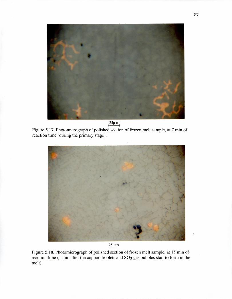
25g m

Figure 5.17. Photomicrograph of polished section of frozen melt sample, at 7 min ofreaction time (during the primary stage).

25[im

Figure 5.18. Photomicrograph of polished section of frozen melt sample, at 15 min ofreaction time (1 min after the copper droplets and SO2 gas bubbles start to form in themelt).

87

88

The reaction rate results indicated that the transition time for 2 1/min of 22% 02 and 78%

Ar, at 1200 °C, is approximately 14 min (refer to Figure 5.6). This means that before 14

min, there should be no copper and gas bubble formation in the melt. At 14 min the

secondary stage commences, for which Reactions (5.19), (5.21) and (5.22) proceed in the

melt, thereby forming copper droplets and SO2 gas bubbles, as can be seen in Figures

5.18-5.23.

It is evident that the metal phase, at 15 min of elapsed reaction time, is in the form of

droplets, of 11±14tm average diameter, as shown in Figure 5.18, rather than precipitates

around the sulphide grain boundaries, as shown in Figure 5.17. This is an indication that

the copper formed after 15 min is the result of the oxidation reaction, rather than the

result of the slow quenching process.

wri -Nu-7

4

_

10011 mFigure 5.19. Photomicrograph of polished section of frozen melt sample, at 25 min ofreaction time.

2511 mFigure 5.20. Photomicrograph of polished section of frozen melt sample, at 25 min ofreaction time.

14 lit - Ifigh4„

410111P 4*,

Oh'

10011 m

Figure 5.21. Photomicrograph of polished section of frozen melt sample, at 35 min ofreaction time.

89

1001.1m1 IFigure 5.22. Photomicrograph of polished section of frozen melt sample, at 40 min ofreaction time.

10011m1^IFigure 5.23. Photomicrograph of polished section of frozen melt sample, at 50 min ofreaction time.

90

91

After 25 min of reaction time, the quantity of copper and gas bubbles increases, as shown

in Figure 5.19. The average copper droplet diameter, of 26±31.tm appears to be larger as

the reaction time elapses. The other important point to note is that there are two types of

copper formation: the large copper droplets, and small random copper droplets that are

associated with the gas bubbles. As suggested by Reactions (5.19), (5.21) and (5.22), the

latter are expected, since they share common reaction sites. The shape of the small

copper droplets appear to be random, unlike the large copper droplets, which are

spherical. Because the melt is spontaneously mixed as a result of surface-tension driven

flows and gas evolution, evidently the small copper droplets agglomerate to form the

larger droplets, as shown in Figures (5.19) and (5.20). From surface observations during

the secondary stage, small numbers of gas bubbles were observed to rise randomly from

the melt on a continuous basis and large quantities, in a boiling fashion, on a less frequent

basis. Due to the fluid dynamics of the system, the size and quantity of gas bubbles with

respect to time cannot be traced in a similar way to the copper droplets. However, when

the sample was extracted just before an incident of intense boiling, in a coincidental

manner, a large quantity of gas was found to be contained by the melt, as shown in Figure

5.21.

Due to the density difference between the metal phase (7.9 g/cm3) and the sulphide phase

(5.5 g/cm3) [113], the copper droplets coalesce and settle to the bottom of the crucible.

The gas bubbles coalesce and rise to the melt surface continuously as well. However, as

mentioned previously, occasionally intense boiling was observed to occur at the melt

surface. During the secondary stage, the appearance of the sulphide phase remained

unchanged until its complete depletion, as shown in Figures 5.18-5.23. Once the sulphide

phase was completely consumed, at the end of the secondary stage, the composition of the

melt approaches that of the metal phase, viz. approximately 98% Cu, 0.95% S and 0.16%

0, at 1200 °C and 1 atm [19]. As shown in Figures 5.24 and 5.25, towards the end of

'p,; " NO%

I%

,- Jeffi C c.

cc* t^°r-

YA`o, • •^• d*31

•.

N't 114;11e:!°^t• ,ivoilW

ert-^.4.-^•c $41T:-'•.:dAt"

v •c-

-0 • .4^.444

6;K • al:,

t:*^! ?:;ts WAt• co r."1"111• 7^• A °. I. C.4

)11',2411^V^d Pt• 't^•'lit,'._

JE^b•

Z11,14,e 7 • 4,11.N4t.._

-7 • a •^• ,

61e^44‘4°Sre'°"

IA^QA.

• • 79gt

ANKA:k. • 3rtt^_Vc.^':;■•°^.41 ^•

92

secondary stage, the melt becomes predominately metallic (brown) containing the

remaining sulphide phase (blue). Referring to the Cu-S binary, ignoring the effect of

oxygen, at 1200 °C, for compositions of less than 1.4% S, the melt consists of the liquid

copper phase such as that shown in Figure 5.26. In Figure 5.26, a polished section of

99.99% pure copper is shown to illustrate the apparent microstructural differences

between pure copper and the copper produced at the end of the secondary stage. For

compositions of greater than 1.4% S, the melt consists of the liquid copper and liquid

copper sulphide phases. Rapid quenching of the 1.4% S sample should result in the

suppression of any sulphide phase segregation, which takes place in the case of

equilibrium cooling. However, due to the use of quartz tubes in the sampling of the melt,

the rate of cooling of the sample, during quenching, appears to have been relatively slow.

As shown in Figure 5.24, the dendritic precipitate of the Cu2S phase (green/blue), in the

matrix of the metal phase (light brown), is the result of equilibrium cooling.

6 .:

1251.1m

Figure 5.24. Photomicrograph of polished section of frozen melt sample, at 60 minreaction time (final reaction time is 70 min).

93

This indicates that the sample was quenched at a relatively low rate of cooling. Thus it is

apparent that the melt consists only of the metal phase, at the sampling time. At the final

reaction time, the composition of the melt is very close to blister copper, of 98.5-99.5%

Cu. The compositional effect on the phase constitutions of the metal phase is shown in

Figures 5.25-5.26.

2511 m

Figure 5.25. Photomicrograph of polished section of frozen melt sample, at 60 minreaction time (final reaction time is 70 min).

25[tm

Figure 5.26. Photomicrograph of polished section of a 99.99% Cu standard sample.

94

95

5.3. Observations of the Bath Surface

Surface observations were useful, not only to investigate the Marangoni effect and gas

bubbles eruptions, but also to gather more qualitative data about the reaction kinetics, and

to aid in the termination of the reaction because surface-tension driven flows were

observed to cease at the end of the secondary stage.

When the copper sulphide bath completely melted under argon, a thin liquid opaque film,

easily broken by movement, was observed to cover the stagnant melt surface evenly, with

the exception of some random shiny areas which appeared to be the sulphide melt, as

shown in Figure 5.27.

Figure 5.27. Bath surface, at 1200°C with top-lancing at 2 1/min of Ar; the blacktriangular area at the top is the tip of the lance appearing out of focus; the right and leftbottom segments of a ring are the inner rim of the crucible; the area within is the opaquefilm covering most of the melt except some random more shiny areas (the sulphide meltsurface). Note the absence of surface movement, due to the gas impingement on thesurface.

Although its chemical composition is unknown, the opaque film appeared to be

immiscible with respect to the sulphide melt. Due to the apparent difference between its

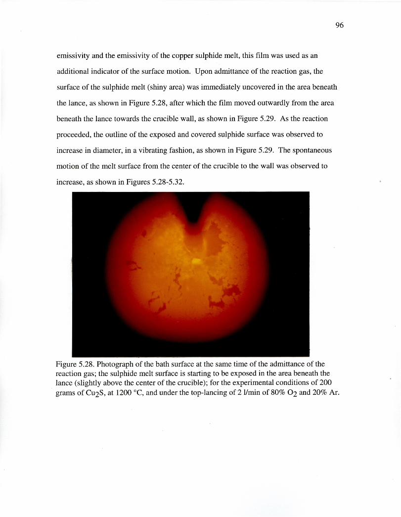
96

emissivity and the emissivity of the copper sulphide melt, this film was used as an

additional indicator of the surface motion. Upon admittance of the reaction gas, the

surface of the sulphide melt (shiny area) was immediately uncovered in the area beneath

the lance, as shown in Figure 5.28, after which the film moved outwardly from the area

beneath the lance towards the crucible wall, as shown in Figure 5.29. As the reaction

proceeded, the outline of the exposed and covered sulphide surface was observed to

increase in diameter, in a vibrating fashion, as shown in Figure 5.29. The spontaneous

motion of the melt surface from the center of the crucible to the wall was observed to

increase, as shown in Figures 5.28-5.32.

Figure 5.28. Photograph of the bath surface at the same time of the admittance of thereaction gas; the sulphide melt surface is starting to be exposed in the area beneath thelance (slightly above the center of the crucible); for the experimental conditions of 200grams of Cu2S, at 1200 °C, and under the top-lancing of 2 11min of 80% 02 and 20% Ar.

Figure 5.29. Photograph of the surface of the bath at approximately 60 s, after theinitiation of the reaction. The film is pushed away from the center of the crucible to thewall, as seen by the further exposure of the sulphide shiny surface.

Figure 5.30. Photograph of the surface at approximately 3.5 min; spontaneous wavymotion of the melt surface is fully developed and the film is entirely pushed towards thecrucible wall, as seen by the full exposure of the sulphide surface. The difference in thecolor of the surface is due to its wavy motion.

97

98

Once the spontaneous surface motion was fully developed, it continued throughout the

duration of the reaction time, as shown in Figures 5.30-5.32. The speed at which the

surface moved, due to the effect of surface tension, was observed to be apparently high

enough to cause the stirring of the whole bath. Due to the motion of the melt surface, the

thermocouple sheath, when immersed in the melt, was observed to continuously vibrate

about its vertical axis, in a pendulum-like motion, creating a clinking noise. Because the

eruption of gas bubbles from the melt surface occurred only during the secondary stage,

the high degree of turbulence is attributed mainly to surface tension-driven flows. In

studying the effects of reaction gas flow rate, reaction gas composition, and reaction

temperature, the general behaviour of the melt surface was observed to be the same.

However, the speed at which the surface moved was observed to be faster with higher

reaction flow rate and composition, as shown in Figures 5.31 and 5.32. On the other

hand, the effect of temperature was not detectable.

Figure 5.31. Photograph of the surface of the bath at approximately 5 min; the oxidationrate results indicated that the transition time for these experimental conditions was 5 min.Note that the film is entirely pushed away from the center of the crucible to the wall.

Figure 5.32. Photograph of the surface of the melt at approximately 21 min; spontaneouswavy motion of the melt surface continues throughout the duration of the reaction time.The oxidation rate results indicated that the final reaction time for these experimentalconditions was 22 min.

Figure 5.33. Photograph of the surface of the melt at approximately 20 min for theexperimental conditions of 200 grams of Cu2S, at 1200 °C, and under the top-lancing of21/min of 22% 02 and 78% Ar. The transition and the final reaction times for theseexperimental conditions are 14 and 70 min respectively.

99

100

At the end of the oxidation reaction, the surface movement was observed to completely

cease, and the film was observed to be pushed to the crucible wall (no surface spreading

is occurring which may be the result of surface tension effects), as shown in Figure 5.34.

Figure 5.34. Photograph of the surface of the melt at approximately 10 min after the endof reaction. At the end of the secondary stage, the surface movement completely ceases.Note the difference in emissivity between the copper surface (shiny reflecting the lancenozzle at slightly above the center of the melt) and the emissivity of the film, at thecrucible wall.

During the secondary stage, bubbles were observed to erupt from the melt surface in a

continuous fashion. Occasional intense boiling was observed to occur at the melt surface

as shown in Figure 5.35. The intensity and the frequency of boiling were observed to

increase with increasing reaction gas flow rate and oxygen content, as shown in Figures

5.35 and 5.36.

101

Figure 5.35. Photograph of the surface of the melt at approximately 14.5 min, under thetop-lancing of 2 1/min of 80% 02 and 20% Ar. Intense boiling at the melt surface, causedby the eruption of SO2 gas bubbles, as a result of the melt reactions.

Figure 5.36. Photograph of the surface of the melt at approximately 14.5 min, under thetop-lancing of 2 1/min of 80% 02 and 20% Ar. Intense boiling at the melt surface, causedby the eruption of SO2 gas bubbles, as a result of the melt reactions.

102

The frequent intense boiling indicates that as the number of gas bubbles increases, the

bubbles coalesce and rise to the melt surface, causing the interruption of surface-tension

driven flow. As discussed in Chapter 6, the effect of this phenomenon, on the transport

conditions, was relatively strong. The break-up of the melt surface causes an increase in

the interfacial area, while the increased surface turbulence causes the enhancement of the

transport conditions.

6. Gas Phase Mass Transfer

6.1. Mathematical Analysis for Mass-Transfer Coefficient

To obtain mass-transfer coefficients from the experimental data, the following

mathematical analysis was undertaken.

^6.1.1.^Material Balance

As the reaction takes place, sulphur is removed from the bath in the form of SO2, thereby

changing the bath sulphur content. The sulphur molar balance on the bath yields the

following.

[rate of S input = 0] – [rate of S output]–

[rate of S consumption = 0] + [rate of S generation = 0]= rate of S accumulation

dN

^

–flso2. A = -dt

^6.1.2.^Flux Equation:

As shown in Figures 5.10, 5.11 and 5.12, the response of the reaction rates to oxygen

content in the gas is characteristic of gas phase mass transfer control. The results shown

in Figure 5.16 also reveal that the liquid phase mass transfer resistance is negligible.

Thus the rate of reaction can be described by the oxygen molar flux, as follows:

k02^b^nino2 =—

RT [Po, – r-o21

^6.1.3.^Equilibrium At Phase Boundaries:

If the chemical reaction rate is fast, the interfacial partial pressure of oxygen must be that

of the equilibrium oxygen pressure, dictated by Reaction (5.18). There are no available

equilibrium data for this reaction; however, since the intercepts of the regression lines in

103

(6.1)

(6.2)

(6.3)

104

Figures 5.10, 5.11 and 5.12 are approximately zero, the partial pressure of oxygen must

be negligible in magnitude, compared to the bulk partial pressure of oxygen.

6.1.4.^Stoichiometry:

The molar ratio of reacted oxygen to evolved sulphur dioxide, a , is calculated as

follows:

(6.4)

During the primary stage, the sulphur removal takes place only as a result of Reaction

(5.18). Since aP is very close to 1.5, thus

oP^2k02nso, = ---L PLif;3 RT 2

(6.5)

During the secondary stage, the experimental results indicate that the ratio of the 02

molar flux to the secondary SO2 molar flux, is approximately 0.96. The corresponding

equation for the molar flux of SO2 in the secondary stage is, therefore, described as

follows:

it' :02 = 0.196 R1(07, p,

02 ^2

6.1.5.^Solution:

In order to develop an expression for the sulphur content of the bath, the first order

differential equation ( Equation (6.2)) is solved by substituting for the respective flux

equations, and integrating between the following limits:

t = 0, N=s A Ps.

t = t* , Ns = N;

For the primary stage the resulting integration is:

(6.6)

Ns 2 kodN s =Â 13(b) dt

Is4^3 RT^0

2 koNs = N'sÂPob .t

3 RT

Similarly, the secondary stage expression is derived as follows:

1 ko APG: [t —Ns = N*s ^

0.96 RT

where t* is the transition time. Thus with gas phase mass transfer control, the bath

sulphur content varies linearly with time. In general terms,

Ns=a+bt^ (6.10)

When compared to Figure 5.4 which exhibits a linear relationship between the measured

moles of sulphur in the bath and time, clearly the oxidation of molten Cu2S is controlled

by gas phase mass transfer of oxygen to the melt surface.

6.2. Experimental Gas Phase Mass-Transfer Coefficient

The gas phase mass-transfer coefficient is calculated from the slope of the plot of sulphur

molar content in the bath vs. time, as follows:

aP RT ANgAP0b2 At

—

as RT AN ;)

;k

-2ÂP,'2 At

Figure 6.1 shows the effect of admitted gas flow rate on the gas phase mass-transfer

coefficient.

(6.11)

(6.12)

105

(6.7)

(6.8)

(6.9)

1

1000 10000

100

106


Figure 6.1. The gas phase mass-transfer coefficient as a function of gas flow rate for theexperimental conditions of 200 grams of Cu2S at 1200 °C, 1.084 atm, 3 mm insidediameter lance, 44 mm diameter of the interfacial reaction area and 10 mm distance fromthe nozzle to the reaction surface; 0 primary measured; A secondary measured,^primary calculated from regression curve (= 0.03 Q0.73), secondary calculatedfrom regression curve (= 0.01 Q0.88).

Although the measured oxygen fluxes for the two stages appear to be identical, their

corresponding gas phase mass-transfer coefficients seem to be slightly different. It can be

seen that this is similar behaviour to the reaction rates, which exhibited greater exponents

for the secondary stage (see Section 5.1.3). The exponents indicate that the relationship

between the gas phase mass-transfer coefficient and the gas flow rate, is stronger in the

107

secondary stage than in the primary stage likely because during the former, gas bubbles

erupt from the melt surface (see Figure 5.35 and 5.36), thereby increasing the gas/liquid

interfacial area. Due to the difficulty of estimating the changes in the reaction interfacial

area, it is not possible to account for this effect. Surface observations of the melt

indicated that the frequency of gas bubbling and the interfacial turbulence were enhanced

by an increase in the gas flow rate and the oxygen concentration in the gas.

In Figure 6.2, the gas phase mass-transfer coefficient is plotted against the partial pressure

of oxygen, from which it appears that there is a slight dependence on the oxygen content.

0^P^I I 11111 1111

0.0^0.2^0.4^0.6 0.8^1.0


Figure 6.2. The gas phase mass-transfer coefficient vs. the partial pressure of oxygen forthe experimental conditions of 200 grams of Cu25, average system pressure of 1.09 atm,3 mm inside diameter lance, 44 mm diameter of the interfacial reaction area and 10 mmdistance from the nozzle to the reaction surface; • primary measured; 0 secondarymeasured, ^ regression line( Equation (5.15)),^ average.

108

Under normal conditions, the gas phase mass-transfer coefficient is effectively

independent of the oxygen concentration in the gas phase; however, owing to the

Marangoni effect, the gas phase mass transfer coefficient slightly increases with

increasing oxygen content in the reaction gas.

k02 = (8.2 ±0.2) + (1.5 ±0.3)13, (6.13)

The average gas phase mass-transfer coefficient, from the primary and secondary stages,

is plotted against the inverse of temperature in Figure 6.3, from which it is clear that the

gas phase mass-transfer coefficient has a slight positive dependence on temperature.

6.2^6.3^6.4^6.5^6.6^6.7^6.8^6.9^7.0

(1 / T) x104 (°K-')

Figure 6.3. The gas phase mass-transfer coefficient vs. the inverse of temperature for theexperimental conditions of: 2000 ml/min of 20-23% 02 and average pressure of 1.08; 0

^

mean of the measured primary and secondary, ^ regression curve (Equation(6.14)).

109

From least squares, the Arrhenius relationship, described by Equation (6.14), yielded an

activation energy of 14±12 kJ/mole, which is a characteristic of mass transfer.

[ 14 ±12kJ/ mole iiln^= ln(3. 3 ± O. 9)O. 0083144 kJ/°K. mole] T

(6.14)

6.3. Gas Phase Mass -Transfer Correlation

The gas phase mass-transfer coefficient is empirically24 related to the transport conditions

of the system via the Sherwood number, Sh. As discussed in Section 2.3.2.1.2, for

laminar top-blown systems, Sh is related to the Schmidt number, Sc, and the Reynolds

number, Re, as follows [48125:

Sh = m(rd dr RenR' Ses'^ (6.15)

Figure 6.4 shows a logarithmic plot of Sh against Re based on the results of this study.

For constant Sc and (rsId), the exponents of Re are 0.73 and 0.88 for the primary stage

and secondary stage respectively, as described by Equations (6.16) and (6.17), which

indicate that the empirical relationships of the Sh-Re are identical to the empirical

relationships of the k02 — Q.

ShP = 0.03Re°^

(6.16)

Shs = 0.02 Ream^

(6.17)

24The transport properties of the gas are considered to be those of the reaction gas mixture, forwhich the calculation procedures are presented in Appendix C.25The Sherwood number, Sh, is the ratio of the total mass transfer to the mass transfer bymolecular diffusion; the Schmidt number, Sc, is the ratio of the momentum diffusivity to themolecular diffusivity and the Reynolds number, Re, is the ratio of the inertia force of a fluid tothe viscous force.

10

0.1

110

10^

1 00^

1000

Re

Figure 6.4. The Sherwood number as a function of the Reynolds number for the topblown conditions of 200 grams of Cu2S at 1200 °C, 1.084 atm, 3 mm inside diameterlance, 44 mm diameter of the interfacial reaction area and 10 mm distance from thenozzle to the reaction surface and Sc = 0.57; 0 primary measured; A secondary measured;^ primary calculated from regression curve (— 0.03 Re0-73); ^ secondarycalculated from regression curve (= 0.02 Re0.88).

From boundary-layer theory [120], and in most mass transfer correlations, the exponent

of the Schmidt number, nsc, is of the order of 1/5-1/3. Since the Schmidt number is a

function of the physical properties of the fluid involved in mass transfer, at room

temperature, the range of Sc is high enough (0.05-5) to allow the determination of its

exponent more accurately from measurements. However, in high temperature systems,

the Schmidt number is only of the order of 0.57-0.9 [48] (in the case of 02-Ar/N2 gas

111

mixtures at 1200-1300 °C, it is 0.57-0.61). In their evaluation of the Sherwood number at

high temperature, Taniguchi et al. [48] assumed that n ^0.5. Similarly, their results

gave the best fit when the exponent of (rid), ns, was -1 for room temperature systems

and -1.5 for the high temperature systems. Figure 6.5 shows a plot of Sh(r.141.5Sc-°-5

against Re from the experimental results obtained in this study.

100

10

1

10^

100^

1000

Re

Figure 6.5. Sh(rs 141)1.5 SC° 5 plotted against the Reynolds number for top-blown

conditions of 02-Ar/N2 onto molten Cu2S bath, at 1200-1300°C, 1.084 atm, 0.56 Sc0.63, 7 rid _C.11, 2-3 mm inside diameter lance, 44 mm diameter of the interfacialreaction area and 10 nun distance from the nozzle to the reaction surface; 0 primarymeasured; • secondary measured; ^ calculated from regression curve (Sh = (0.64±0.07)(d/rs) 1 -5 sc0.6Re(0.79±0.06)); ^ secondary calculated from regression curve (Sh=(m= 0.74) ((d/rs)1-5Sc"Re036, from decarburization of liquid iron, after Taniguchi et al.[48])).

112

The resulting correlation is as follows:

Sh = (0.64 ± 0.07)(r, 1 d) 5 Sc° 5 Re(°79±°°6)^

(6.18)

By comparison Taniguchi et al. [48] found the exponent of Re to be 0.66 for room

temperature systems and 0.76 obtained from the rate of decarburization of liquid iron, (of

greater than 0.2 wt% carbon). The results presented in Figure 6.5 clearly agree with the

experimental measurements of Taniguchi et al. for Re = 13-1500, r s/d = 1.6-5 and Hid =

0.4-30, for which (Sh = m (r s/d)-1-5Sc0.5Re°3 6). In the system under study these values

are Re = 33-147, r s/d = 11-7.3 and Hid = 3.33-5, and the value for m that gives the best

agreement is 0.74. As shown in Figure 2.7 (a), m appears to vary slightly with the type of

system. For the water-N2-NH3 system, it is 0.27 and it is 0.53 for the toluene-N2 system.

Although the exponents of the correlation obtained from the decarburization of liquid

iron are closer to those of the current system, m appears to differ greatly. For the

decarburization of liquid iron, m = 0.27 ± 0.05, while it was found to be 0.74 ± 0.01 for

the current system.

For the purpose of analyzing the oxidation kinetics of molten Cu2S, Equation (6.18) was

used in the prediction of the gas phase mass-transfer coefficient. Since all of the

apparently relevant parameters are in agreement with those obtained from systems of gas

mass transfer control [45-48], this correlation was accepted in the prediction of the gas

phase mass-transfer coefficient.

Table 6.1 shows the effect of lance diameter on the gas phase mass-transfer coefficient.

The lance nozzle-diameter appears to be an important parameter in the gas phase mass-

transfer. Where a 33% decrease in the diameter results in an approximately 20% increase

in the gas phase mass-transfer coefficient, the correlation provides a better prediction

when nsc is -1.5 than when it is -1, as shown in Table 6.1.

113

Table 6.1. The effect of the lance diameter on the gas phase mass transfer coefficient.These runs were conducted at 1200 °C and average oxygen content of 21%.

Q/a- d rdd Hid

k02

m= 0.64,n, = -1.5

and nRe = 0.79

_k02

m = 0. 25, ns = –1

and nRe = 0.78

Icf)2

measuredkns

•-.2

measured

(ml/min) (mm) (cm/s) (cm/s) (cm/s) (cm/s)

1480 3 7 3 6.57 6.49 5.95 6.45

1520 2 11 5 7.57 23.12 7.42 7.40

6.4. Sensitivity Analysis of the Effect of the Interfacial Area on Gas Phase

Mass-Transfer Coefficient

In top-blown systems, the reaction interfacial area is a function of the flow characteristics

of the jet and the diameter of the crucible. For highly turbulent systems, the reaction

interfacial area may be considered to be the area of the paraboloid, outlined by the jet

impingement area, as follows:

A = —Tc [D. + 4Hc13/2 —116

(6.19)

In laminar flow systems in a certain crucible diameter range, the reaction interfacial area

is assumed to be the cross-sectional area of the crucible. The experimental measurements

and the numerical computations of Taniguchi et al. [47-48] revealed that for laminar flow

conditions, the reaction interfacial area can be assumed to be the cross-sectional area of

the crucible, as shown in Figure 6.6. From a numerical solution of the gas phase flow

equations, and from visualizing the flow pattern of the gas phase by a tracer (TiC14) [47],

it was deduced that this assumption was acceptable.

114

Figure 6.6. Computed streamline patterns and concentration profiles at u = 200 ink(laminar flow) (after Taniguchi et al. [48]); (a) streamline patterns iv, (b) concentrationprofiles Y.

From Equation (6.18), the variation in the predicted gas phase mass-transfer coefficient is

related to the variation in the reaction interfacial area as follows:

Sko, = --3

(0.64)7t3/4D^crISC Re° 794^02 -Ar

SA(6.20)

The variation in the experimentally determined gas phase mass-transfer coefficient is

related to the variation in the interfacial reaction area as follows:

= N 02 RT SA (6.21)Pbo2 A2

Due to the rising gas bubbles frequently erupting from the melt during the secondary

stage, the reaction interfacial area may vary to an uncertain extent. In order to investigate

the effect of this possible variation on the gas phase mass-transfer coefficient, a

100

10

1

115

sensitivity analysis was carried out using Equations (6.20) and (6.21). The results are

shown in Figure 6.7 and indicate that a 20% variation in the area, results in approximately

15% and up to 21% uncertainties in the estimation of the measured and predicted gas

phase mass-transfer coefficients respectively.

1000^ 10000


Figure 6.7. The sensitivity of the gas phase mass-transfer coefficient to the reactioninterfacial area, for the experimental conditions of 200 grams of Cu2S at 1200 °C, 3 mminside diameter lance, 44 mm diameter of the interfacial reaction area and 10 mm distanceform the nozzle to the reaction surface; 0 mean, determined from measurement (A =15.14 cm2); .. uncertainty bars (OA = 3.028 cm2 equivalent to 20 % variation), ^predicted (A = 15.14 cm2);^ predicted uncertainty limits (SA = 3.028 cm2equivalent to 20 % variation).

116

6.5. Sensitivity Analysis of the Effect of Temperature on Gas Phase Mass-

Transfer Coefficient

In the calculation of transport coefficients, such as the gas phase mass-transfer coefficient

or the heat-transfer coefficient, the temperature at which the thermophysical properties

are computed, is often considered to be the mean film temperature. In systems of high

gas velocity and a very steep thermal gradient between the reaction region and the gas

delivery regions (such as the lance nozzle), it is feasible to consider the temperature of the

gas to be at a mean temperature between the hot zone and the gas. However, in the

system under investigation, the lance extends over a distance of approximately 400 mm in

which the thermal gradient inside the reaction tube26 is relatively gradual. This allows the

gas to reach a temperature close to that of the hot zone. Due to the exothermic heat of

reaction, depending on the gas flow rate and oxygen content in the gas, the temperatures

of the bath and the gas were observed to increase by up to 60 °C, relative to the start of

reaction. Due to the expected small effect of temperature on the reaction rate, and to the

short life of the alumina thermocouple sheaths in the vicinity of the reaction, it was not

possible to obtain a continuous temperature measurement for some of the runs. However,

reasonably sufficient data, on the thermal behaviour of the reaction system, have been

gathered27 to reveal that the temperature rise is proportional to the increase in the oxygen

content and gas flow rate of the reaction gas, as given by Equations (6.22)-(6.24) and

shown in Figures 6.8 and 6.9.

26Refer to Section 4.1.1 (Figure 4.1).27Melt and gas temperature measurements are provided in Appendix D.

70

117

60

50

40

0E 30

00 20

10

-1 0 I I II""1""1""1""I""1""1""

0

^

^500 1000 1500 2000 2500 3000 3500 4000


Figure 6.8. The temperature change, due to the heat of reaction, as a function of thereaction gas flow rate; LI melt temperature change (the tip of the thermocouple sheath waslocated at the center of the melt), ^ regression line (Equation (6.22)); 0 gastemperature change (the tip of the thermocouple sheath was located at the same height asthat of the lance nozzle28); ^ regression line (Equation (6.23)).

28Due to the poor heat transfer conditions between the thermocouple and the gas, the gastemperature measurements are expected to be lower than the actual temperature (for moreaccurate measurements to be conducted, a suction thermocouple should be used).

70

60

50

a)czi 40

a)EE-4g 30CI)

c‘C9

U20

10

118

'

^I^''

0^

20^

40^

60^

80^

100

Oxygen Content (%)

Figure 6.9. The temperature change, due to the heat of reaction, as a function of thereaction gas oxygen content; o gas temperature change (the tip of thermocouple sheath

^

was located at the same height as that of the lance^nozzle), ^ regression line(Equation (6.24)).

^ATmelt = —8 +0.018Q:^ (6.22)

^

= —15+0.014Q:^ (6.23)

t‘Tgas = —7.3 + 0. 8002)^ (6.24)

119

Using the estimated correlations for AT, a temperature sensitivity analysis was carried

out to investigate the effect of temperature uncertainty on the calculated values of the gas

phase mass-transfer coefficients. The mean temperature of the melt and the gas was

calculated from the estimated correlations, and it was used to compute the gas phase

mass-transfer coefficients, as shown in Figures 5.11-5.12. The gas phase mass-transfer-

temperature sensitivity analysis indicated that a ±50°C uncertainty in temperature can

result in approximately ±4% uncertainty in the calculation of the gas phase mass-transfer

coefficients, which is within the tolerance limit, as shown in Figures 6.10 and 6.11.

According to the gas phase mass-transfer corelation, the gas phase mass-transfer

coefficient is expected to be slightly dependent on the gas composition mainly through

the Schmidt number. However, at high temperatures, the contribution of Sc is small

compared to Re. When increasing the oxygen content in the reaction gas, the temperature

change and surface-tension driven flows are higher. From the above discussion, it

appears that the effect of temperature on the gas phase mass transfer coefficient is

negligible. The experimental results suggest that the dependence of the gas phase mass-

transfer coefficient on the oxygen content in the gas is slightly higher than predicted by

the correlation, as shown in Figure 6.11. It seems that there is only a small dependence,

for compositions of approximately 50% 02 and higher. Since the temperature effect is

insignificant, this dependence is attributed to the effect of surface-tension driven flows

and the eruption of gas bubbles. Surface observations indicated that the spontaneous

motion is increased with increasing oxygen content of the reaction gas (see Section 5.3).

100

10

1

120

1000^ 10000


Figure 6.10. The sensitivity of the gas phase mass-transfer coefficient to temperature, forthe experimental conditions of 200 grams of Cu2S at 1200 °C, 20-26% 02, 3 mm insidediameter lance, 44 mm diameter of the interfacial reaction area and 10 mm distance fromthe nozzle to the reaction surface; 0 primary measured (T = 1200 °C); CI secondarymeasured (T = 1200 °C); ^ predicted (T = 1200 °C); 111 primary measured (mean);0 secondary measured (mean);^ predicted (mean).

0^8ao9

0a^

I .^1Îî^ .^.^1Î

121

12

10

0.0^0.2^0.4^0.6^0.8^

1.0^1.2


Figure 6.11. The effect of reaction gas composition on the gas phase mass-transfercoefficient, for the experimental conditions of 200 grams of Cu2S, average systempressure of 1.09 atm, 3 mm inside diameter lance, 44 mm diameter of the interfacialreaction area and 10 mm distance from the nozzle to the reaction surface; 0 primarymeasured (T = 1200 °C); 0 secondary measured (T = 1200 °C), predicted (T =1200 °C); ^ predicted (mean temperature form Equation (6.26)).

7. Mathematical Modeling and Theoretical Predictions

Having presented and discussed the experimental findings of this work, it is conducive to

examine these findings theoretically via mathematical modeling of the oxidation reaction.

A theoretical description of the oxidation of molten Cu2S bath is essential for further

understanding of this process and for the support and validation of the experimental

measurements. In this chapter, a detailed formulation of the mathematical model is

presented. Using the experimental results, validation and sensitivity analyses of this

model are also examined. To provide a theoretical description of the oxidation of molten

copper sulphide, the oxidation path and the oxidation rates of molten copper sulphide

baths are discussed in terms of the model predictions.

7.1. Mathematical Model

7.1.1.^Assumptions

1. The melt is vigorously mixed and consists of a homogeneous solution of

S2-, 02- and Cu+ ions (sulphide phase), during the primary stage. The

formation of the copper-rich phase (metal phase) takes place during the

secondary stage, as a product of the melt reactions only29. The metal

phase remains in equilibrium with the sulphide phase until the complete

depletion of the sulphide phase at the end of the secondary stage (end of

the oxidation reaction).

2. The oxidation reaction is controlled by the gas phase mass transfer of

oxygen to the melt surface.

122

29Note that Reaction (5.18) is referred to as the surface reaction and Reactions (5.19), (5.21) and(5.22) are referred to as the melt reactions.

123

3. The melt at the end of the primary stage is assumed to be the equilibrium

composition of the sulphide phase saturated with oxygen at the given

temperature and pressure.

4. The melt at the end of the secondary stage is assumed to be copper

containing equilibrium amounts of oxygen and sulphur.

5. Equilibrium conditions are assumed to prevail at the gas-liquid interface.

The surface reaction apparently has a large negative Gibbs free energy

with a large equilibrium constant. Thus under gas phase mass transfer

control, the interfacial partial pressure of oxygen is very small compared

with the bulk partial pressure of oxygen. Due to the absence of

thermodynamic data for the activities of [S2-] and [021 in the melt, it is

not possible to calculate the equilibrium partial pressure of oxygen

dictated by the surface reaction. The molar flux of oxygen can be

described as follow:

ko r bno2 =--IP

RT 2

6. The transport properties of the gas are assumed to be those of the reaction

gas mixture i.e. Ar+02.

7. The transition period from the primary stage to the secondary stage is very

small and was assumed to be negligible.

8. Due to the effect of bubbles rising from the melt during the secondary

stage, the reaction interfacial area is increased causing the overall rate to

increase by a minor amount. This was apparent from the gas phase mass-

transfer coefficient determined in the secondary stage which was found to

124

be slightly higher than that of the primary stage". However, since the

measured gas phase mass-transfer coefficient was found to increase only

by about 4% in the secondary stage, it is assumed that the gas phase mass-

transfer coefficient remains constant throughout the reaction duration.

9. The reaction interfacial area is assumed to be the cross-sectional area of

the crucible.

10. Isothermal conditions prevail throughout the duration of the reaction time.

In spite of the fact that the temperature of the system was observed to

increase at the beginning of the reaction time and to remain constant

throughout the duration of the experiments (as a result of the exothermic

reaction), this assumption was adopted because of the small effect that the

temperature has on the overall reaction rate.

11. The gas phase is assumed to be at the same temperature as the liquid

phase. Due to the low value of the specific heat capacity of gases and to

the nature of this reaction system31, it is safe to assume that the heat

transfer to the reacting gas, in the hot zone, is instantaneous.

7.1.2.^Reaction Mechanism and Flux Equations

7.1.2.1.^Primary Stage

The formation of copper does not take place until the sulphide phase is saturated with

oxygen. This is due to the relatively high oxygen solubility in molten copper sulphide, of

approximately 1.47 wt% at 1200°C and 1 atm pressure. During the primary stage, the

sulphide melt is partially desulphurized and oxygen saturated until its composition has

reached approximately 80.83 wt% Cu, 17.7 wt% S and 1.47 wt% 0 at 1200 °C and 1 atm

30For details about the calculation of the measured gas phase mass transfer coefficient, refer toSection 5.1.5.1.31The basis for this assumption has been discussed in detail in Section 5.1.5.2.

[s 21V

DistanceA

Gas Phaseb

PO2

\

Concentration>

Liquid Phase

13`02

SO2 02

/

125

[19]. This process is controlled by the gas phase mass transfer of oxygen to the melt

surface, where it reacts with sulphide melt, in the absence of any other reactions as shown

in Figure (7.1), according to Reaction (5.18).

Due to the Marangoni effect at the bath surface, the sulphur and oxygen concentrations in

the melt are assumed to be constant throughout the liquid phase i.e. the liquid phase mass

transfer resistance is virtually non-existent. Therefore, as mentioned above, the

expression describing the reaction rate is Equation (7.1).

44 mmFigure 7.1. Schematic diagram of the primary stage reaction system; (1) alumina lance;(2) , vigorously mixed molten sulphide as the result of surface tension driven flows(Marangoni effect); (3) schematic diagram of the reaction gas flow pattern; (4) aluminacrucible.

7.1.2.2.^Secondary Stage

Immediately upon the melt composition reaching the transition composition of 80.83 wt%

Cu, 17.7 wt% S and 1.47 wt% 0 at 1200 °C and 1 atm, the secondary stage commences.

126

During the secondary stage, the copper formation reactions (Reactions (5.19), (5.21) and

(5.22)) take place beneath the surface throughout the melt. Simultaneously with the

formation of copper, oxygen and sulphur dissolve in the metal, according to Reactions

(5.21) and (5.22), to yield about 98.89% Cu, 0.95% S and 0.16% 0. Reaction (5.19) is

triggered when the oxygen concentration at a nucleating site has slightly exceeded the

equilibrium concentration of the sulphide phase. Once this reaction initiates, the

formation of copper droplets and SO2 gas bubbles provides more reaction sites to keep

the sulphide phase in equilibrium with the metal and gas phases. Because the reactions

are electrochemical, ionic mobility and electron transport tremendously retard the liquid

phase mass transfer resistance (on the microscopic scale). Growth and coalescence of the

gas bubbles are followed by their rise to the melt surface. These phenomena provide an

enhancement of the stirring action caused by the surface-tension driven flow. Due to the

surface eruptions caused by the rising gas bubbles, the gas-liquid interfacial reaction area

increases and enhances the overall reaction rate by up to 6%. The frequency of rising gas

bubbles has been observed to increase with increasing flow rate oxygen partial pressure in

the reaction gas. Spontaneous mixing of the melt is further enhanced by the coalescence

and settlement of the copper droplets. However, because the copper droplets and the gas

bubbles exist only during the secondary stage, the melt is believed to be mainly mixed by

the effect of surface-tension driven flow phenomena.

The metal phase at the bottom of the bath grows at the expense of the sulphide phase until

the secondary stage is ended, at which time all of the sulphide phase is consumed. The

secondary stage reaction system is shown schematically in Figures 7.2 and 7.3, from

which, it is apparent that the reaction conditions of the secondary stage are slightly

different from those of the primary stage. However, the rate limiting step remains the

mass transfer of oxygen in the gas phase above the bath.

Suiphide Phase

Metal Phase

127

Distance

Gas Phase

02

Concentration

Suiphide Phase

I

Metal Phase

(1)

44mm Figure 7.2. Schematic diagram of the secondary stage reaction system; (1) alumina lance;(2) alumina crucible; (3) schematic diagram of the reaction gas flow pattern; (4) sulphidephase; (5) metal phase; 0 sulphur dioxide gas bubbles; copper droplets.

Figure 7.3. Secondary stage; (1) surface reaction interface for Reaction (5.18); (2)reacting sulphide phase (according to Reactions (5.19), (5.21) and (5.22)); (3) sulphide-metal interface (showing the net metal phase formation rates); Suiphide phase; 0sulphur dioxide gas bubbles; copper droplets.

128

7.1.3.^Equilibrium at Phase boundaries

It is safe to suggest that equilibrium conditions prevail at the melt surface i.e. at the gas-

liquid interface. Therefore the interfacial partial pressure of oxygen is assumed to be the

equilibrium partial pressure of oxygen, as dictated by the thermodynamics of Reaction

(5.18) and at least one order of magnitude smaller than the bulk partial pressure of

oxygen. Then Equation (7.1) is transformed as follows:

.^k02no2 ..==^2 PoRT 2

Due to the spontaneous mixing of the melt, there is no concentration gradient in either of

the liquid phases. The oxygen- and sulphur-saturated metal phase is in equilibrium with

both the gas and sulphide phases.

Since the amount of copper formed, due to Reactions (5.19), (5.21) and (5.22), is

saturated with oxygen and sulphur, the moles of oxygen and sulphur dissolved in copper

can be related to the moles of copper formed via their equilibrium relationships, as

follows:

N0 =m 0[{100 —[% Si^

100 1 c. i[[% Cu

N =^N cu M cal00

s

M s[[100 —{100

700]cut[% s]cu

1]—[% O]cd

N cisM 0,100

(7.2)

(7.3)

(7.4)

129

By differentiating Equations (7.3) and (7.4) with respect to time and noting that

[% s] and [%0], are constants, relationships between the rate of copper formation

and the rates of oxygen and sulphur dissolution in copper are obtained,

N cu A 1 0,100No =

as follows:

(7.5)m^100

u0[[100—[%s]ct

mc.100=Let^On,

100 (7.6)m0[[100—[%Si cu][ [%pica

N = Ocu NCu^ (7.7)

N cu M100Ns = (7.8)100A^ -]_[%0]cu]s[[100—[%O]cui[ [%s]cw^1

Ain, 100let^So, =(7.9)100

Ais^6] [%0L[[100^[%^c 1[u^[%S]cu

N s = ScuNcu^ (7.10)

The oxygen and sulphur concentrations in the metal phase are calculated from the

equilibrium measurements of J. Schmiedl [19], as given by the following equations32:

32Note that Ps02 (in Equations (7.11)) is in mmHg.

130

[%oicu = 10 (-1.4-(1278/T))^y.p 2SO2

[%cu] =10(2+(2""

[ % S] ^100 —[% Cu] --[%O]cu

where the SO2 partial pressure, in the melt, is equal to the system pressure, Ps, and the

average sulphide phase static head on an SO2 gas bubble located at a mid-distance from

the surface, Pst, as follows:

PS02 = P Pst^ (7.14)

As seen in Figures 5.18-5.23, the sulphide phase contains the freshly formed copper

droplets throughout the secondary stage. Thus, as the metal phase is formed within the

sulphide phase, the sulphide melt density is assumed to be the average value for the

sulphide phase and metal phase densities, as given by the following equation:

(Hicu2s)(Pcu,s+Pcu Pt = 2^2

(7.15)

7.1.4.^Stoichiometry


Reaction (5.18) is the surface reaction that takes place when a copper sulphide melt,

having a stoichiometric Cu2S composition33, is brought in contact with oxygen gas. Melt

surface observations and micro-examination of quenched bath samples, obtained during

the primary stage, indicated very clearly that there is no bubble formation during this

period. The stoichiometric relationship between the molar flux of oxygen and the

primary molar flux of sulphur dioxide can be obtained from Reaction (5.18) as given by

33The Cu-S binary, at 1200 °C and 1 atm, indicates that liquid copper sulphide can range incomposition from 20 to 22.19 wt % sulphur (refer to Section 2.2).

Equation (7.16). By substituting for n 02 from Equation (7.2) in Equation (7.16), anP

expression for nso, is obtained as follows:

0 P^1nS02 = —

12—no2

3

P^2 k02nso2

3 RT 2

131

(7.16)

(7.17)


During the secondary stage, Reaction (5.18) is no longer the only reaction that is

responsible for the sulphur removal from the sulphide phase. Reactions (5.19) and (5.21)

take place in the melt, contributing further to sulphur ion removal. By maintaining the

sulphide phase composition below the transition composition, the melt reactions sustain

the chemical potential for reaction (5.18). Due to the dissolution of oxygen and sulphur

in copper, the proportions of Reactions (5.18) and (5.19) are not known. Therefore it is

not possible to formulate theoretically a direct stoichiometry between the no2 and ns02.

The overall reaction for the copper formation can be represented by Reaction (7.18).

Therefore the rate of copper ion consumption from the sulphide phase can be directly

related to the rate of copper generation, as given by Equation (7.19).

{Cul+ = ((Cu))

0N cu* = N

(7.18)

(7.19)

From the stoichiometry of Reactions (5.21) and (5.22), the relationships between the rates

of oxygen and sulphur ions consumption from the sulphide phase are related to the rates

of oxygen and sulphur dissolution in the metal phase, as follows:

o2- = o^ (7.20)

N s2- = Ns^ (7.21)

132

7.1.5.^Material Balance

For simplicity, this mathematical model will be constructed to describe each of the two

stages in a distinct manner. For the primary stage, a material balance on the sulphide

phase yields the formulation of a model that predicts the sulphur and oxygen contents of

the bath. For the secondary stage, a material balance on the sulphide phase shall be

performed to develop expressions for the rates of copper, oxygen and sulphur

consumption from the sulphide phase. The description of the metal phase generation can

be obtained by performing a material balance on the metal phase. By combining the

results of the material balances on the sulphide phase and the metal phase an overall

description of the bath, during the secondary stage, can be formulated.


7.1.5.1.1.^Sulphur Balance

Assuming that there is no concentration gradient of sulphur in the bath, a molar balance

for sulphur in the bath yields the following:

[rate of S2- input = O]-[rate of S2- output]+

[rate of S2- generation = OF [rate of S2- consumption = 01=^(7.22)rate of S2- accumulation

Since the sulphur removed from the bath is in the form of SO2, the rate of S2- output

from the bath is directly related to the SO2 molar flux as follows:

. Prate of S2- output = ns02. A^ (7.23)

Substituting for Equation (7.23) in Equation (7.22);

. P^dN ,2_— n SO2 . A = '

dt(7.24)

133

7.1.5.1.2.^Oxygen Balance

Similarly for oxygen;

[rate of 02- input ] - [rate of 02- output ] +

[rate of 02- generation = OF [rate of 02- consumption = 0] =^(7.25)

rate of 02- accumulation

Oxygen is dissolved in the bath as 02- and is removed from the bath in the form of S02•

Therefore the rate of 02 input is the product of the molar flux of 02 and the cross-

sectional area of the crucible, as given by Equation (7.26). The rate of 02 output can be

expressed in terms of the molar flux of SO2, as given by Equation (7.27).

rate of 02- input = 2 I; 02. A^ (7.26)

. P

rate of 02- output = 2nso2• A^ (7.27)

Substituting Equations (7.26) and (7.27) in Equation (7.25), the following expression is

obtained:

.^. 13^dN 2_2 no2. A —2 ns,92. A = ^°

dt (7.28)


7.1.5.2.1.^Sulphide Phase

7.1.5.2.1.1. Sulphur Ion Balance

As shown in Figure 7.3, some of the sulphur reacts to form SO2, according to Reactions

(5.18), (5.19), and some dissolves in the metal phase according to Reaction (5.21). A

material balance for the sulphur yields the following:

dN 2_. s^A^. r.,

— fl s02 • A — IV s2 = Sdt

(7.32)

134

[rate of S2- input = O]- [rate of S2- output] +

[rate of S2- generation = 0]— [rate of S2- consumption ] =

rate of S2- accumulation

The rate of sulphur output is related to the secondary SO2 molar flux as follows:

rate of S2- output = ns02. A

(7.29)

(7.30)

rate of S2- consumption = Ns2-^ (7.31)

Substituting Equations (7.30) and (7.31) in Equation (7.29), we obtain the following

expression:

7.1.5.2.1.2. Oxygen Ion Balance

The oxygen input to the sulphide phase is a known quantity, given by the transport

conditions of the reaction system. As outlined in Figure 7.3, some of the oxygen reacts

with the sulphur at the melt surface, according to Reaction (5.18); some of it is removed

from the bath in the form of SO2, according to Reaction (5.19), and some of it dissolves

in the metal phase, according to Reaction (5.21). Hence, the oxygen balance yields the

following:

[rate of 02- input ] - [rate of 02- output] +

[rate of 02- generation = 0] — [ rate of 02- consumption i =^(7.33)

rate of 02- accumulation

The rate of oxygen input is related to the 02 molar flux, as follows:

rate of 02- input = 2 n 02 • A^ (7.34)

The rate of oxygen output is related to the secondary SO2 molar flux, as follows:

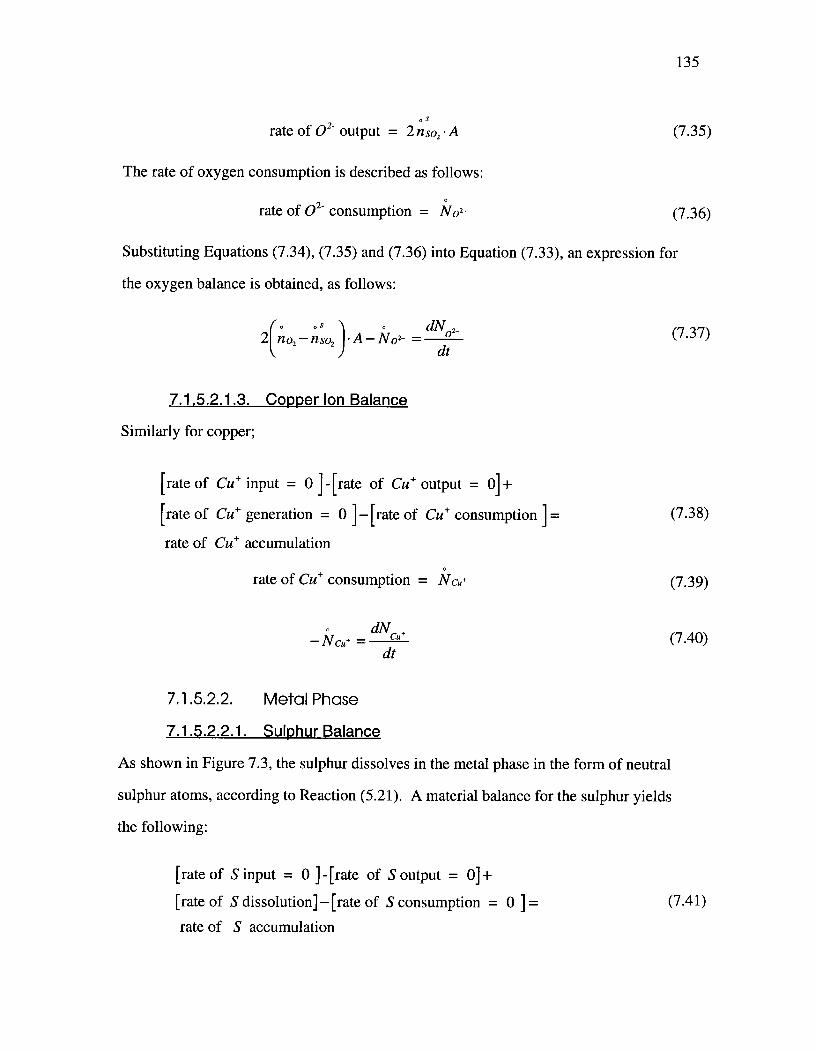
135

„ srate of 02- output = 2 ns02. A^ (7.35)

The rate of oxygen consumption is described as follows:

rate of 02- consumption = No2-^ (7.36)

Substituting Equations (7.34), (7.35) and (7.36) into Equation (7.33), an expression for

the oxygen balance is obtained, as follows:

^. ^,s^0^

dN ,

^

2,(n02- ^nso,)• A — N o2 =^dt

7.1.5.2.1.3. Copper Ion Balance

Similarly for copper;

[rate of Cu+ input = 0 ]-[rate of Cu+ output = 0] +

[rate of Cu+ generation = 0 ] — [rate of Cu+ consumption ] =

rate of Cu+ accumulation

(7.37)

(7.38)

rate of Cu+ consumption = N cw.^ (7.39)

.^dNCI4+— N Cu+ =

dt(7.40)

7.1.5.2.2.^Metal Phase

7.1.5.2.2.1. Sulphur Balance

As shown in Figure 7.3, the sulphur dissolves in the metal phase in the form of neutral

sulphur atoms, according to Reaction (5.21). A material balance for the sulphur yields

the following:

[rate of S input = 0 ] - [rate of S output = 0]+

[rate of S dissolution]— [rate of S consumption = 0 ] =^(7.41)

rate of S accumulation

136

rate of S dissolution = Ns

k s . dNsdt

7.1 .5.2.2.2. Oxygen Balance

Similarly for oxygen;

[rate of 0 input = 0 ]- [rate of 0 output = 0]+[rate of 0 dissolution] — [rate of 0 consumption = 0 ] =rate of 0 accumulation

rate of 0 dissolution = No

k 0 . dNodt

7.1.5.2.2.3. Copper Balance

The copper material balance is described as follows:

[rate of Cu input = 0 ] - [rate of Cu output = 0]+[rate of Cu generation ]— [rate of Cu consumption = 0 ] =rate of Cu accumulation

(7.42)

(7.43)

(7.44)

(7.45)

(7.46)

(7.47)

rate of Cu generation = Ncu^ (7.48)

.^dNNcu = cu

dt(7.49)

137

7.1.6.^Mathematical Solution


For 0 t t , where t* is the transition time, expressions for the moles of sulphur and

oxygen in the bath are developed by integrating Equations (7.24) and (7.28) subject to the

following initial condition:

at t =0, N52 = N's„ and NO2 = 0

Arca-P

dN 2 = nS02 • Ai dts0

(7.50)

PBecause nso2 # f (Ns2_ ), the expression for the moles of sulphur in the bath is given by

the following equation:

N = —(n sP +s2-^2 • _ _

Equation (7.28) is integrated subject to the initial condition, as follows:

No2-.

dN 02_ = 2(no2—nso2)• AS dt

(7.51)

(7.52)

PBecause nso, # f(NO2) and no, # f(NO2_), the expression for the moles of oxygen in

the bath is given by the following equation:

0 PN0 = 2(no2— nso2}4 • t- (7.53)

PSubstituting for nso2 and no2 in Equations (7.51) and (7.53), the final formulations for

the sulphur and oxygen in the bath are developed.

02 k bN2 = Ns12_ —(—

3 RT2 A P°2 *t(7.54)

138

NO2_ =(3-RkC)7,2 A Pob2)• t^ (7 .55)

The primary rates of sulphur removal and oxygen dissolution, as functions of the oxygen

partial pressure, are derived as follows:

dNsp,_ = (2 ko2A)pb

dt^3 RT ) 02

dNop,_ =12 ko,A)pbdt^3 RT ) 02

(7.56)

(7.57)

Substituting for the gas phase mass-transfer coefficient expression (Equation (6.18)) in

Equations (7.56) and (7.57), the primary rates of sulphur removal and oxygen dissolution

can be expressed in terms of the reaction gas flow rate, as follows:

,^0.79 ]dNsP2_ = ( 2 P/12 AI O. 64 Do, _Ar ( d r \I 1-1, g [M.- P g j^Q0.79

dt^3 RT^d^rs^p gD02_Ar 4g

0.79]dNop2_ =r 2 Pict A O. 64 Do2 _Ar " dl .11 11g ^(7cd-

, P g)^Q0.79

dt^3 RT )^d^rs^p gD02-Ar 411.g

(7.58)

(7.59)

At the transition time, the sulphide bath composition is dictated by the equilibrium

conditions of the system, as given by the following equations:

N* u* m cul00N s* 2_ =^

1 100 ^1—[% GI] cu2s]m s[[100 —[% 0] cu2s .1[{% S]cu2s

(7.60)

No* 2- =^

[% clmo[[100— [% S ] cu2s

100 ^11_{% s]1cu2

s^cu2s

N* M 100ca

(7.65)*^Nis2_ N*s2_t =

r2k02^b)

3 RT A P°2 )

139

(7.61)

The oxygen and sulphur concentrations in the sulphide phase at the transition time are

calculated from the equilibrium measurements of J. Schmiedl [19], as given by the

following equations:

[%°1CU2S = 10(-2+0013/T)) pY2 (7.62)so2

[%Cutu2s = 79.605 + 0.26 x 10-12 T4^ (7.63)

[%Slcu2s = 100 —[% Cu] [% O]Cu2s^ (7.64)

Substituting for the conditions at the transition time in Equation (7.54) or Equation

(7.55), an expression for the transition reaction time can be developed as given by the

following equation:

During the primary stage, the moles of copper ions in the bath are constant; therefore the

moles of copper ions (N.+ ) at transition are the initial moles of copper in the bath.

Using Equations (7.54) and (7.55), an expression for the bath weight as a function of

time, during the primary stage, can be expressed as follows:

WP (t) = w(o) +[M0 — Ms .1[—=-2 A 13,;',]• t3 RT^2

(7.66)

140

An expression for the rate of weight change in the primary stage as a function of the

oxygen pressure can be derived by differentiating Equation (7.66) with respect to time, as

follows:

0 P^2 ko AW =[111° —Ms] 3 R2 T PCb'2

The rate of weight change can be expressed in terms of the reaction gas flow rate as

follows:

° P 2^0.641002-ArPob2 ^ incrpg )0.79 0.79W {Mo Ms]^

QRT P gD02-Ar 4114


Unlike the primary stage, the secondary stage does not offer a direct stoichiometricos

relationship between the nso2 and n02. The following equations are to be solved

simultaneously for the unknown reaction rates and the final reaction time34.

Sulphide phase sulphur balance:

dN 2_n SO2 • A — N S2 = S

dt

Sulphide phase oxygen balance:

2(no2—nso2)• A _NO2 = dA 1 n2

dt

Sulphide phase copper balance:

dN— N0 = Cu

dt

(7.67)

(7.68)

(7.32)

(7.37)

(7.40)

34The unknown reaction rates and the final reaction time are constants in a determined system ofequations that can be solved simultaneously.

141

Sulphur solubility in the metal phase:

= S^

(7.69)

Oxygen solubility in the metal phase:

NO2- = Ocu Ncu.^ (7.70)

Experimental results indicated that all reaction rates are constants, i.e. they are neither

functions of composition nor functions of time. Integrating Equations (7.32), (7.37) and

(7.40) for the following initial conditions:

at^,^Ns, = Pts2_

NO2 = N*o2_ and N+ = N*cu^cu+

N2 ^0 s

dN s,_ = +s02. A+ N s2-jf dtN s2-^ t.

(7.71)

*

N2 = NS , —S

s^ r^*1nso2. A+ N S2-)• Lt^t (7.72)

No2- o s ]t

f dNo,_ 42 (n o2— so2)• A— N 02-^dt (7.73)N.

02-^ t*

0 sNO2 = N*^+ [2(n02— nso2)A— No2- • [t — (7.74)

N

dN^= —^cu+^dtcu+(7.75)

N*

Ncu+ = N., —

jvc.. [ t (7.76)

At the end of the reaction time, the sulphide phase is completely depleted, i.e.

142

at t=tfN =0'^s2-^'No 2 = 0 and N

Cu+ = 0

-

Substituting for these final conditions in Equations (7.72), (7.74) and (7.76), permits the

solution for the unknown reaction rates35, as follows:

. S^0^,

N;2_ — (nS02 ' A + Ns2- )•[tf — ] = 0 (7.77)

.^. sNo*2_ +[2(no, —nso, )44 — k02- ] • [tf —t*1= 0^ (7.78)

N*— N° cu+[tf — ]= 0cu+

(7.79)

Solving for {tf — t*] form Equation (7.79) and substituting in Equations (7.77) and (7.78),

the following is obtained:

o s,,^,, ro^N,_ NC

n so, . I-1 ± IV S2" = - *Nc

u+

0^0 s *^0

2(no2— n SO2 )A — No2- = N o2_ AT cu+

N*Cu+

(7.80)

(7.81)

Using Equation (7.69) to solve for Nce and substituting in Equations (7.70), (7.80) and

(7.81), the following is obtained:

0

.^ Or. Ns2-No2 . ,Ii (7.82)

SCu

35Note that the unknowns are the constants in a system of equations, in which all of thedependent variables are known.

143

*. s^.^NN s2-nso2. A+ N^s 2_ (7.83)s2^=^*

NCu+

SCu

.^. s^.^N*^N s2-2(no2— ns02)A—

2N02 = (7.84)

N* +Scu^cu

Substituting for Equation (7.82) in Equation (7.84), and solving for iVs2-, as follows:

o s.

N S2 =N* +Scu nso2. ACu (7.85)

[N* 2 — N* S ]s -^cu+^cu

o^o s2N*^S,-, (no —nso),4cu+^,,,,^2^2

iVs2 (7.86)=[6°CUNC*U+

_N]]Equating Equations (7.85) and (7.86), the following expression is obtained:

0 s

n so2 =^1 (7.87)no2

1 1+[ [OcuN c* u+ — N 0* 2_]]

r2[AT;2_ —Nc*.+Scui

Substituting for no2 in Equation (7.87), an expression for the molar flux of SO2 is

obtained as given by the following equation:

° s^ 1^k02^pb(7.88)=n so,

1+r[OcuArc*a+ — N*02_ 1 RT^°2

r21 N*s2_ — Nc*u„ Scu ]

Expressions for the consumption rates of sulphur, oxygen and copper ions from the

sulphide phase are derived as follows:

144

Ar°^2/Vc% Scu A^k, pbiv s2 = r r^ -21.21.N;2_ — NC* u*Scul+[OcuNc* u+ — No* ,]]RT

2NC* u*OcuA^ko2NO2- = r r^ pb

[21.N; — A Icsu*Scu]±[OcuNc* u, No* ]] RT '92

^2N* + A^k 02 pb^Cu ^02N cu+ = r r1.2[N*s2- NL,Scu [()CuN*cu*^

2_]] RT

The expression for the final reaction time is derived as follows:

RT

^

tf =[3N` 2_ — N* — N* 2_ + Nu* ^— 2S Icu L^0 bS^S^0^cu^2Ak 2 • Po2

By integrating Equations (7.43), (7.46) and (7.49) for the following initial condition,

expressions for the metal phase growth can be derived:

at t =0, Ns =0,

No = 0 and Nc. = 0

(7.89)

(7.90)

(7.91)

(7.92)

Ns

dNs = Ns dt

Ns= Ns•[t —

No^tidNo= No dt0

No= No•[t—t1

Arc„^t

dku = NCu dt0

(7.93)

(7.94)

(7.95)

(7.96)

(7.97)

145

Ncu = Ncu•Lt —^ (7.98)

By adding the respective equations of the sulphide and metal phases, and utilizing the

relationships of Equations (7.19), (7.20) and (7.21), expressions for the secondary moles

of copper, sulphur and oxygen in the bath can be derived as follows:Os

=N2 —nso,• A -[t — (7.99)

0^S

AIL = N*o2_ 2(no2—nso,),4•{t — t*I^ (7.100)

Ns = N*cu^cu+ (7.101)

Substituting for no„ nso2 and t* in Equations (7.99)-(7.101), the expressions for the

secondary moles of sulphur and oxygen (total) are given by the following equations:

2[Ns*,_ — Nc*u„Scu]= N*,_ + r^

s^1.2N;2_ — N 0* 2_ + Nc* u,.[Ocu— 2Sc.a]]

2[N*,52_ — Nc* u+Scui ATL N*02_^r

[2N*,_ — No*,_ + Arc*a+ [On, — 2Scu]]

3 rN,,^N*, (7.102)[21-^s^s

(k0,APcb,2)

RT

_^_1^3[Arls, — N*s22k, AP b,

t (7.103)-2RT

By differentiating Equations (7.102) and (7.103) with respect to time, expressions for the

rate of sulphur and oxygen removal from the bath in the secondary stage as a functions of

the oxygen partial pressure are derived as follows:

^dN^F^2[N*s2_ — Arc* u,Scu]^k02A)pb

^

dt^[2N*s2_ — N*02_ + Nc* u,[0cu —2Scu]] RT )(7.104)

^d„,^2[N*s2_ — Nc*.„,] ^lir 21CO2A)pt:^dt^{2N*s2_ — N2 + c*u+[Ocu —2S0u]]^RT^02

(7.105)

146

Expressions for the secondary rates of sulphur and oxygen removal in terms of the

reaction gas flow rate are derived as follows:

0.79O. 64700,_„^[tgdr,dN's'^2[N;2 — I c*u.Scul

dt^[PN*52_ —^+ NTcd-P g (7.106)

dN0.

..,[0cu-2ScujQ0.79

RT^p gD02 _Ar

— N cs a+ scu]

41. g

dt1]

[2 Nss,_ — N os 2_ + N cs u+{Ocu —2s]](7.107)

gdrs g)x [1.287CD02_ArP73,^(1Cd3p

RT^p gD02_Ar^411g^

]Q0.79

An expression for the bath weight as a function of time in the secondary stage is derived

as follows:

_^c*Ws (t) = W(e) — [2M0 —{2M0—Mstr^

2[N*e — Nu+Scu*^*^ .0^

(7.108)

X1.2 N s2_ No2_ Nc*u+ [Ocu 2Scujj

[-3 [Ni — Ns^11(02AP(b)2 t]2 s2-^s2-^RT

The rate of weight change as a function of the oxygen partial pressure in the secondary

stage is derived by differentiating Equation (7.108) with respect to time as follows:

IV *1;2_ — A Iu+Scul= 2M0—{2M0—Mst[^

cs ^ko A-2 ^pb

[2 N:s2_ — N*02_ ± N*cu+ [Oct, — 2S cu]]]( RT)

02(7.109)

Similarly, the rate of weight change in the secondary stage is expressed in terms of the

reaction gas flow rate as follows:

147

2[N*s,_ — A TW = [2M0 — [2M0

AI]—^s r

— N + [Ocu — 2Scu ]](7.110)

_ArPob2 179gdr,X[0.64700,

RT

(Tcd3pg iQ0.79

pgD02-Ar^411 g

7.2. Model Validation

The general criteria for the model validity are comparison of its prediction of the sulphur

and oxygen contents for the two stages and their time domains to measurements from the

laboratory experiments. From Equations (7.54) and (7.55), the primary sulphur and

oxygen molar contents were calculated; the reaction transition time was calculated from

Equation (7.65); and the secondary sulphur and oxygen molar contents were calculated

from Equations (7.102) and (7.103). These predicted results were plotted along with the

corresponding measured values for typical runs, as shown in Figures 7.4-7.5.

The apparent curvature of the measured oxygen content is due to experimental scatter. It

is important to note that the accuracy of the sulphur content measurement is higher than

that of the oxygen content measurement36. The relative disagreement between the

predicted and the measured results is attributed to the errors associated with the input

parameters to the model (reaction gas flow rate, reaction gas composition and the

measured pressure of the system) and the estimation of the gas phase mass transfer

coefficient. The model predictions, however, appear to be in very good agreement with

the measured results, for the employed range of the reaction gas flow rate, as shown in

Figure 7.4.

36The sulphur content was determined by the acid-base titration method, which is a moreconventionally accurate method than the gas flow rate measurement technique, which was usedin the determination of the oxygen content. As explained in Section 4.1.5.5, in general, the errorin the measurement of the reaction gas flow rate is proportional to the flow rate.

12080^1000^20^40^60

1.4

1.2

1.0

0.4

0.2

0.0

148

Time (min)

Figure 7.4. Comparison of model predictions to measurements of the sulphur and oxygencontents in the bath as a function of time at a constant reaction gas composition and forthe range of reaction gas flow rate of 1480-4055 ml/min; for the experimental conditionsof: 200 grams of Cu2S of: 22% 02 and 78% Ar, at 1200 °C,^ predicted for 1480ml/min; Emeasured sulphur content for 1480 ml/min; 0 measured oxygen content for1480 ml/min; ^ predicted for 2006 ml/min; 0 measured sulphur content for 2006ml/min; A measured oxygen content for 2006 ml/min; — — — predicted for 4055ml/min; + measured sulphur content for 4055 ml/min; • measured oxygen content for4055 ml/min.

Similarly for the reaction gas composition range, the predicted and measured results are

as shown in Figure 7.5.

10^20^30^40^50^60^70^80

149

Time (min)

Figure 7.5. Comparison of model predictions to measurements of sulphur and oxygencontents in the bath as a function of time at a constant reaction gas flow rate and for therange of reaction gas composition of 22-78% 02; for the experimental conditions of: 200grams of Cu2S of: 2000 ml/min, at 1200 °C,^ predicted for 22% 02; 0 measuredsulphur content for 22% 02; 0 measured oxygen content for 22% 02; — — — predictedfor 35% 02; o measured sulphur content for 35% 02; • measured oxygen content for35% 02;^ predicted for 78% 02; A measured sulphur content for 78% 02; +measured oxygen content for 78% 02.

150

The relative deviation from the measured results, at the highest reaction gas composition

conditions, is mainly attributed to the effect of surface-tension driven flows 37 . It is

evident, however, that the model provides an acceptable predictability for the

experimental range of reaction gas composition.

Considering the error involved in the measured results, the model predictions appear to be

well within the experimental uncertainty of the measured values. It is therefore

reasonable to state that the model predictions are in good agreement with the overall

range of the measured results.

7.3. Model Sensitivity

Since all of the reaction parameters are set or read with some degree of uncertainty, it is

inevitable that the input variables to the mathematical model carry some degree of error.

In order to examine the effect of these uncertainties on the model predictions, and to

isolate as much as possible the experimental error from the model deviations, this

analysis is carried out using the results of a run that appears to contain the least relative

errors.

7.3.1.^Temperature

As shown in Figure 7.6, the uncertainty in the temperature evidently has a very minor

effect on the oveall model predictions. An error of ±50 °C (2.5%) results in less than 1%

error in the sample weight prediction and less than 6% error in the prediction of the

transition time.

37The effect of surface-tension driven flows was found to be higher with oxygen content in thereaction gas; as a result, the transport conditions are enhanced beyond the accountability of themodel (see Figure 6.2).

205

200

195

^

190 ^

E

^

E5, 185 ^to

i 180 —*8

^

1 175 ^gcl

^

170 ^

165

160

155 ' '

0^10

" I '20^30^40^50^60

Time (mm)

151

Figure 7.6. Model-predicted sensitivity of transient bath weight to bath temperature38 forthe experimental conditions of; ^ predicted for 1200 °C; 0 measured at 1200 °C;— - — - predicted for 1150 °C;^ predicted for 1250 °C.

7.3.2.^Pressure

Due to the pressure head created by the SO2 absorber, the measurements were conducted

under pressures of slightly higher than that of the atmospheric pressure viz., 1.05-1.112

atm. For systems such as that under study, however, it is well known that the pressure

38The experimental conditions of this run, used in all of the sensitivity analyses, are: 200 gramsof Cu2S, 2000 ml/min of 35% 02 and 65% Ar

152

has a minor effect on most thermodynamic properties [114]. As shown in Figure 7.7, the

results of this sensitivity analysis indicated that a 5% uncertainty in the pressure of the

system results in less than 3% error in the prediction of the reaction transition time and a

less than 2% error in the prediction of the sample weight.

^205 ^

200

195 —

^

190 ^

R., 185....,Zto 180

^

1 175 ^(4

^

170 ^

^

165 ^

^

160 ^

^

155 ^

0

" I "

10^20^30^40^50

Time (mm)

60

Figure 7.7. Model-predicted sensitivity of transient bath weight to total pressure,predicted for 1.09 atm; 0 measured at 1.09 atm; — - - — predicted for 1 atm; predicted for 1.15 atm.

205

200

195

190

I ::

c9 i85.4 iso.8.= 175'c'Elal

170

165

160

155

0 20

" I I

30 40 50 60

153

7.3.3.^Reaction Gas Flow Rate

As shown in Figure 7.8, the results of the model-reaction gas flow rate sensitivity analysis

indicated that a 5% error in the reaction gas flow rate results in less than 4% error in the

prediction of the reaction transition time and less than 0.8% error in the prediction of the

sample weight.

Time (min)

Figure 7.8. Model-predicted sensitivity of transient bath weight to flow rate of admittedgas; ^ predicted for 2000 ml/min; 0 measured for 2000 ml/min; — - - —predicted for 1900 ml/min; ^ predicted for 2100 ml/min.

" I '' I ",

205

200

195

..^175'401gq

170

165

160

155

0^10^20^30^40^50^60

154

7.3.4. Reaction Gas composition

In this analysis, a 5% uncertainty in the reaction gas composition was found to result in

less than 6% error in the prediction of the reaction transition time and less than 2% error

in the prediction of the sample weight, as shown in Figure 7.9.

Time (min)

Figure 7.9. Model-predicted sensitivity of transient bath weight to composition ofadmitted gas;^ predicted for 35% 02; 0 measured for 35% 02; — - - —predicted for 33% 02;^ predicted for 37% 02.

In the experiments, the reaction gas mixture was obtained by metering each gas stream

using a separate rotameter. Thus the error in the reaction gas composition is

approximately the sum of the errors of the two readings. Since the reaction rate is

195

190

g 185to

-:a..0 180*Ei

175121

170

165

160

155

155

directly proportional to the reaction gas composition, its error contribution is expected to

be higher than that of the reaction gas flow rate.

7.3.5.^Reaction Interfacial Area

If the error associated with the reaction interfacial area was 5%, then the corresponding

errors were 5% and 1% in the predictions of the reaction transition time and the sample

weight respectively, as shown in Figure 7.10.

205

200

0

" I '' '

10^20 30^40^50 60

Time (min)

Figure 7.10. Model-predicted sensitivity of transient bath weight to bath surface area;^ predicted for 15.14 cm2; c.), measured for 15.14 cm2; — - - — predicted for14.38 cm2;^ predicted for 15.90 cm2.

156

7.4. Theoretical Predictions

7.4.1.^Oxidation Path

As presented and discussed in Chapter 5, gas analysis measurements and gravimetric

measurements revealed that the oxidation reaction of molten copper sulphide proceeds

according to two distinct stages, during which the rates are constant, as shown in Figures

5.5 and 5.6. The fact that these two independent measurements are in general agreement

is evidence of their validity. The melt composition at transition and the molar ratio of

reacted oxygen to removed sulphur (a) are independent of reaction conditions (see Table

5.1).

By eliminating time from the expressions for the molar sulphur and oxygen contents

(Equations (7.51), (7.53), (7.99) and (7.100)), the relationship between the sulphur and

oxygen contents are found to be independent of the oxidation kinetics as given by the

following equations:

= Nis — Arf,

[N* 2_ — Sc N* rM = N;+ s^u cu+ IN — N*02_1

Al*, — OcuN*cu_0 -

(7.112)

Although the experimental scatter is considerable, experimental measurements are in

agreement with the predictions of Equations (7.111) and (7.112) as shown in Figure 7.11.

The experimental results indicate very clearly that the oxidation path is controlled

primarily by the thermodynamics of the Cu-S-0 system. From Figure 7.11, the predicted

results indicate that the effect of temperature on the oxidation path is minimal, where a

100 °C increase in temperature causes a slight shift in point b and appears to have no

effect on point c.

Transition Pointa

>1)0^- <>A - X X +O 0 •^fii>^X

^

0 •^'X,Primary Stage^0^• 4+

• X°0 + A0

A°''

• 0

•

•A• A

AA •

X0+

•0

Secondary Stage

II" Il""1""I'"Il""1"

0

A><

157

25

20

0

0.0^0.2^0.4^0.6^0.8^1.0^1.2^1.4^1.6^1.8Cu

wt% Oxygen

Figure 7.11. The sulphur content as a function of the oxygen content in the bath, showingthe oxidation path of molten copper sulphide, ^ predicted at 1200 °C and 1 atm;^ predicted at 1300 °C and 1 atm; measured at 1200 °C and 24 % 02, 0 1480ml/min, A 1755 ml/min, + 1987 ml/min, 0 2006 ml/min, x 4055 ml/min; measured at1200 °C and 2510 ml/min of 23 % 02; measured at 1200 °C and 2000 ml/min, • 27 %02, • 35 % 02, El 46 % 02, • 64 % 02•

Based on the findings of the current work and on earlier thermodynamic studies of the

ternary system, the oxidation path of Cu2S is constructed as shown in Figure 7.12.

Primary StageOxidation Path

19.6% S17.7 % S and 1.47 % 0

Liquid Metal Phase

((Cu))1.33 % S g

f^1.97 % 0

Wt % S^ Wt % 0

Secondary StageOxidation Path

20 dLiquid Sulphide Phase

((Cu2S))

21.72 % S

/

158

Cu

Figure 7.12. Selected portions of the Cu-S-0 isothermal section, showing the oxidationpath of molten Cu2S at 1200 °C and 1 atm (points b and c are after Schmiedl [19]; pointsd, e, f and g are after Elliott [201). Note that the dashed lines outlining the metal andsulphide phases are assumed.

As stated in Section 5.1.3.2, gas analysis measurements yielded 16.94 ± 0.10% and 1.37 ±

0.07% for the sulphur and oxygen transition concentrations respectively. Rottmann and

Wuth [71] found that the melt oxygen content at the end of the primary stage is 0.6%.

Peretti [10] suggested that, based on the Cu-S binary phase diagram, in the Peirce-Smith

159

converter, the second step of the copper-making reaction starts when the melt

composition is about 19.4% sulphur. Peretti, however, ignored the effect of oxygen by

considering the melt to be a binary system. According to the present work, the binary

assumption can be misleading in studying the reaction mechanism of the oxidation of

copper sulphide. The 1300 °C isothermal section, shown in Figure 2.3, indicates that the

sulphur and oxygen concentrations at saturation in Cu2S are approximately 18.59% and

1.38% respectively. At 1200 °C and 1 atm, the equilibrium measurements of Schmiedl

[19] yielded 17.7% and 1.47% for the sulphur and oxygen solubilities in Cu2S

respectively. From comparing the measured transition composition to the equilibrium

composition of sulphur and oxygen in the melt, clearly the melt composition at transition

is that of the equilibrium composition of oxygen and sulphur. Therefore, during the

primary stage, the melt is partially desulphurized and oxygen saturated without any

formation of copper according to path a-b in Figure 7.12. Once the melt reaches point b,

the chemical potential for the formation of the metal phase is attained. An increased

degree of desulphurization accompanies the metal phase formation which takes place

according to path b-c, as shown in Figures 7.11 and 7.12.

As discussed in Section 5.1.3.2, the average value for aP = 1.46 permitted the postulation

of Reaction (5.18) as the principal reaction in the primary stage. In the formulation of the

mathematical model, this postulate was implemented in deriving the relationships

between the reaction rates of the primary stage. As shown in Figures 7.4 and 7.5, the

model predictions of the primary stage are in good agreement with the measured results.

This can best be seen by concentrating on the prediction of the transition point. It is clear,

therefore, that Reaction (5.18) is the only reaction that takes place during the primary

stage. It is very important to note that obtaining a large number of relatively accurate

measurements permitted the calculation of a statistically valid mean for a", from which it

was possible to postulate Reaction (5.18). Although the time duration of the primary

160

stage is only about 20-25 % of the total time of the oxidation reaction, the understanding

of the chemical reactions of the primary stage is very crucial to the comprehension of the

secondary stage.

During the secondary stage, the molar ratio of reacted oxygen to removed sulphur was

found to be as = 0.96 ± 0.052. At first glance this might seem to be an indication that

the actual ratio is unity. However, this can be a very misleading judgment. As discussed

above, because of the reactions are electrochemical in which the dissolution of oxygen

and sulphur in copper, according to Reactions 5.21 and 5.22, is accompanied by electron

transfer, the degree of desulphurization during the secondary stage is further enhanced. It

is important to note that, as explained in Sections 5.1.3.2 and 7.1.2.2, without considering

the electrochemical nature of the system it would not have been possible to account for

the oxygen and sulphur in the metal phase.

7.4.2.Ôxidation Rates

7.4.2.1.Ôxidation Rate as a Function of Gas Flow Rate

From the mathematical model, the oxygen gas phase mass transfer rate is related to the

reaction gas volumetric flow rate as follows:

^0 . 6470,92_ ArPob2Î1gd1ç [7cc13p g)° 79^0 70N0, = ^

RT P gD02-Ar^41.14 g(7.113)

For the oxidation reaction to be gas phase mass transfer limited, the oxygen reaction rate

must be equal to the oxygen gas phase mass transfer rate, predicted by Equation (7.113).

In Figure 7.13, the predicted oxygen reaction rate is compared to the measured oxygen

reaction rate, from which the theoretical prediction appears to be in good agreement with

measured rates.

0.001

1000 10000

0.100

161

Gas Flow Rate (mlhnin)

Figure 7.13. Oxygen reaction rate (No, ) as a function of reaction gas volumetric flow ratefor the experimental conditions of: 200 gram samples, 1200 °C, 23 % 02 and averagepressure of 1.08 atm,^ predicted ; 0 primary measured; • secondary measured.

0.1

0.001

1000 10000

162

In Figure 7.14, the measured and predicted sulphur removal rates (Equations (7.56) and

(7.58)) are plotted against the gas flow rate. As expected, since the sulphur removal rates

are limited by gas phase mass transfer, the predicted and measured rates appear to be in

good agreement.


Figure 7.14. Sulphur removal rate (Ns) as a function of reaction gas volumetric flow ratefor the experimental conditions of: 200 gram samples, 1200 °C, 23 % 02 and averagepressure of 1.08 atm;^ primary predicted; 0 primary measured;^secondary predicted; 0 secondary measured.

-

163

The predictions of Equations (7.68) and (7.110) and the measured rates of weight loss

were predicted and plotted against the admitted gas flow rate in Figure 7.15. Considering

the experimental scatter, the predicted measured results appear to be in general

agreement.

10

0.01 ^1000 10000

Gas Flow Rate (mUmin)

Figure 7.15. Rate of weight loss (W) as a function of reaction gas volumetric flow ratefor the experimental conditions of: 200 gram samples, 1200 °C, 23 % 02 and averagepressure of 1.08 atm; primary predicted; El primary obtained from gas analysis;• primary obtained from gravimetric measurement; ^ secondary predicted; 0secondary obtained from gas analysis; • secondary obtained from gravimetricmeasurement.

0.07

0.06oo

3E 0.05 â)CEcit) 0.04 ^

P4o2ki 0.03 â)

19td)

0

0.01

0.00

0.0

' I "0.2^0.4^0.6^0.8


0

1.0

164

7.4.2.2.Ôxidation Rate as a Function of Gas Composition

As shown in Figure 7.16, the predicted and experimentally determined oxygen reaction

rates are plotted against the partial pressure of oxygen.

Figure 7.16. Oxygen reaction rate (No, ) as a function of oxygen partial pressure for theexperimental conditions of: 1200 °C and 2000 ml/min; predicted; 0 measuredprimary; <> measured secondary.

In a linear fashion, as shown in Figure 7.17, the measured oxygen reaction rate appears to

deviate from the predicted rate of oxygen gas phase mass transfer for oxygen partial

pressures of greater than 0.11.

o

0

165

20

18

16

14

0.0^0.2^0.4^0.6^0.8^

1.0


Figure 7.17. Percent increase in gas phase mass transfer as a function of oxygen partialpressure for the experimental conditions of: 1200 °C and 2000 ml/min,^regression line; 0 determined from measurement.

This deviation is attributed to the increase in the gas phase mass-transfer coefficient, due

to surface tension-driven flows (the Marangoni effect), which were observed to increase

with the partial pressure of oxygen. In mathematical terms, the percent increase in gas

phase mass transfer, C, likely due to the Marangoni effect, was found to correlate to the

partial pressure of oxygen as follows:

C = (22.7±3.6)P0', —(2.7±1.9)^ (7.114)

166

Because, the gas phase mass-transfer coefficient was calculated from a correlation which

does not account for the increase in the transport conditions due to surface-tension driven

flows, the predicted reaction rates are less than the measured reaction rates.

As discussed in Chapter 5, if the reaction is to be controlled by gas phase mass transfer

the sulphur and oxygen molar contents in the bath must be linear with time.

Experimental results presented in Chapter 5 and the mathematical validation in Chapter 7

established that the rate controlling mechanism of the oxidation reaction of molten Cu2S

is gas phase mass transfer (see Figures 5.4, 7.4 and 7.5).

The rates of sulphur removal are directly proportional to the partial pressure of oxygen, as

described by Equations (7.56) and (7.104). In Figure 7.18, the measured rates of sulphur

removal were plotted against the partial pressure of oxygen along with the theoretical

predictions of Equations (7.56) and (7.104). In a similar behaviour to the oxygen reaction

rates, the rates of sulphur removal appear to be influenced by the increased degree of gas

phase mass transfer. In general, however, there is a reasonable agreement between the

predicted and measured rates of sulphur removal, which is an additional evidence that the

rates of sulphur removal are limited by the rates of oxygen gas phase mass transfer.

0.07

167

00.06

E 0.05ooE2,1 0.04

74oE 0.030

r4,..

',2r4= 0.02c4

0.01

0

0.2^0.4^0.6^0.8^

1.0


0.00

0.0

Figure 7.18. Sulphur removal rate (dNsIdt) as a function of oxygen pressure for theexperimental conditions of: 1200 °C and 2000 ml/min,^ primary predicted; 0primary measured; ^ secondary predicted; 0 secondary measured.

0.8 1.00.0^0.2^0.4^0.6

0

0

2.0

1.8

1.6

0cal0.8r:4

0

0.4

0.2

0.0 "I"^IIII"I"

Increase in the reaction rate with oxygen concentration in the reaction gas, in the

oxidation of molten Cu2S, was also exhibited by the experimental results of Rottmann

and Wuth [71], as shown in Figure 7.19.


Figure 7.19. Oxygen reaction rate (N o,) as a function of oxygen pressure for theexperimental conditions of: 1500 grams of Cu2S under the top-lancing of high velocityjets of 02-N2 gas mixtures at 1250 °C, nozzle pressure of 5.4x105 N/m2, nozzle diameterof 1 mm, nozzle to bath distance of 65 mm and crucible inner diameter of 100 mm;^ predicted (after Rottmann and Wuth [71] (based on gas phase mass transfer ofoxygen through a viscous sub-layer)); 0 measured (after Rottmann and Wuth).

168

8vis, = U0.9g,max

2 9 v 0 .9 x 0.1

RTD02-N2 AP02no, = (7.116)

169

As discussed in Section 2.4, Rottmann and Wuth measured the reaction rates of the

oxidation of molten Cu2S for different oxygen concentrations in the bulk gas at 1250 °C.

In their prediction of the reaction rates, Rottmann and Wuth assumed that the reaction is

limited by the oxygen diffusion in a viscous sub-layer of thickness 8. Using a

correlation for the thickness of the boundary layer at a plate exposed parallel to a

turbulent stream, they calculated 8 as follows:

(7.115)

from which the rate of oxygen reaction was calculated as follows:

Because they did not measure the reaction rates for a range of gas flow rates, it is not

possible to validate the assumption of diffusion through a viscous layer and in turn

determine the validity of Equation (7.116). It is likely, however, that the predicted

reaction rates are linear with the oxygen pressure in the gas phase. Assuming that the

actual reaction rates are very close to those predicted by Rottmann and Wuth, it is

suggested that the deviation exhibited by the measured results is due to increased surface-

tension driven flows with oxygen concentration in the admitted gas. The percent increase

in the gas phase mass transfer was similarly correlated to the partial pressure of oxygen as

follows:

= (29 ±4)137,2 + (12 ± 2)^ (7.117)

in which, the slope is slightly higher than that in Equation (7.114). It is therefore,

suggested that, due to the Marangoni effect, the gas phase mass transfer conditions are

enhanced with increasing oxygen concentration in the reaction gas phase. As discussed in

Section 2.5, increases in mass transfer, due to the Marangoni effect, have been observed

170

to occur in many systems [56,82,84,99,101,121]. In the oxidation of molten Cu2S, as

shown in Section 5.3, there is an overwhelming evidence that surface-tension driven

flows play an important role in the overall reaction rate kinetics. By stiffing the bath,

surface-tension driven flows virtually eliminate any liquid phase mass transfer resistance,

as shown in Figure 5.15. As the radial movement of the surface is increased with higher

concentrations of oxygen in the gas phase, the mass transfer conditions are likely to

increase as the moving liquid causes further drag of the gas, thereby, enhancing the

reaction rate beyond the values accounted for by ordinary transport conditions.

7.4.2.3.^Oxidation Rate as a Function of Temperature

From Equation (7.2), the rate of oxygen reaction is inversely proportional to temperature.

The predicted and measured oxygen reaction rates are plotted against temperature in

Figure 7.20. Although the gas phase mass-transfer coefficient is positively dependent on

temperature, the predicted oxygen reaction rate appears to have a slight negative

dependence on temperature, as shown in Figure 7.20. In general, however, it can be

stated that both the measured and predicted oxygen reaction rates are effectively


In comparing Equations (7.56) and (7.104) theoretically, the temperature dependence of

the rate of sulphur removal during the secondary stage is greater than that during the

primary stage. In Equation (7.104), the secondary molar ratio of reacted oxygen to

removed sulphur, as, is a function of the equilibrium concentrations of the melt, as

described by the following equation:

as . 1+ RocuNc*., —

which yields 0.9169 and 0.9250 fora' at 1200 and 1300 °C respectively. Conversely, the

primary molar ratio of reacted oxygen to removed sulphur dioxide, a'', is 1.5

(independent of temperature).

N*02_ ]/2[N*5,2_ — SGUNL,]] (7.118)

171

(1 / T) x104 (70

Figure 7.20. Oxygen reaction rate (No2) as a function of temperature for the experimentalconditions of: 2000 ml/min of 20-23 % 02 and average pressure of 1.08 atm,^primary predicted 22 % 02; 0 primary measured; • secondary measured.

In Figure 7.21, the predicted and measured rates of sulphur removal are plotted against

temperature, from which it appears that measured and predicted results are in agreement.

The primary rate of sulphur removal seems to have a similar behaviour to that of the

oxygen reaction rate, but the secondary rate of sulphur removal appears to be virtually


0.100

172

8-

8

•••00

0

••

0.001 ^ '^' I ' '

6.0^6.2^6.4^6.6 6.8^7.0^7.2

(1 / 7') x104 (°K-1)

Figure 7.21. Sulphur removal rate (dNsIdt) as a function of temperature for theexperimental conditions of: 2000 ml/min of 20-23 % 02 and average pressure of 1.08atm,^ primary predicted 22 % 02, secondary predicted 22 % 02; 0primary measured; • secondary measured.

100

10

173

7.4.3.^Oxygen Utilization

The oxygen utilization as a function of gas flow rate is shown in Figure 7.22, from which

it appears that very high reaction efficiencies are attained in the oxygen-Cu2S system.

This is consistent with the observed oxygen utilization in the Peirce-Smith converter.

100^

1000^

10000


Figure 7.22. Oxygen utilization as a function of reaction gas volumetric flow rate for thetop-blown conditions of: 200 grams of Cu2S at 1200 °C, 1.08 atm, 23% 02, reactioninterfacial diameter of 44 mm, lance nozzle diameter of 3 mm and lance nozzle to initialinterfacial area of approximately 10 mm;^ predicted; 0 measured.

To obtain valid kinetic measurements of heterogeneous reaction systems in laboratory

tests, reactants must be supplied at rates beyond their rates of consumption by the reaction

174

at the given experimental conditions. From Figure 7.22, the predicted oxygen curve

indicates that the limit for obtaining useful kinetic measurements is 750 ml/min i.e. below

this value the oxidation reaction rate is higher than that of the rate of oxygen supply.

Industrial processes in which gas-liquid reactions are involved, the utilization of the

reaction gas is of high economic importance. It is important that the reaction gas

efficiency be as high as possible. Since however, the high efficiency is accompanied by

lower reaction rates, the optimization of a given process may dictate that the gas

utilization be much lower than can be attained.

175

8. Summary and Conclusions

The primary objective of this work was to investigate the oxidation kinetics of molten

copper sulphide under top-blown conditions. The major findings of this work can be

summarized as follows:

1. The oxidation reaction of molten copper sulphide takes place according to two

distinct stages.

2. During the primary stage, the melt is a single phase, being partially desulphurized and

becoming oxygen saturated, according to the surface reaction as follows:

[s2 ]+ % (o2 ) = (so2) +[o2- ]

3. Upon saturation of the melt with oxygen, the secondary stage commences, during

which the following reactions in the sulphide phase produce metallic copper:

[52]+ 2[01+ 6[Cu] = (S02)+6((Cu))

[S1 +2[Cul = [S]((co) +2((Cu))

[01 + 2[Cul = [0]((c)) + 2((Cu))

(5.18)

while the surface reaction involving gaseous oxygen continues to take place until the

end of the secondary stage.

4. The rate of sulphur removal and oxygen dissolution during the primary stage were

found to be independent of sulphur and oxygen contents in the melt. Similarly, the

rates of sulphur and oxygen removal during the secondary stage are independent of

sulphur and oxygen contents in the melt.

5. The rate controlling mechanism in the oxidation of molten Cu2S is gas phase mass

transfer of oxygen to the melt surface; the oxidation rate was found to be directly

176

proportional to the partial pressure of oxygen in the reaction gas. From the

experimental data obtained in this work, the gas phase-mass transfer coefficient was

correlated to experimental variables via the Sherwood number, Sh, the Schmidt

number, Sc (0.56 5. Sc 0.63), the Reynolds number, Re (33 5 Re 300), the radius

of the crucible, rs, and the diameter of the lance nozzle, d (7 rid 11), as follows:

Sh = (0.64 ± 0.07)(rs/d) Sca5 Re (0.79±0.06)^ (6.18)

6. Surface-tension driven flows (Marangoni effect) were observed to take place during

the oxidation reaction. As a result transport conditions at the gas-liquid interface

were slightly enhanced. The degree of surface-turbulence was observed to be a

relatively strong function of the oxygen content in the reaction gas, while the gas flow

rate was observed to cause only a slight increase. The effect of temperature on

surface-tension driven flows was undetectable.

7. In a continuous fashion, the eruption of small numbers of gas bubbles from the melt

surface was observed to take place during the secondary stage, while at random time

intervals, occasional intense boiling was observed to occur as well. The intensity and

frequency of boiling were observed to increase with increasing gas flow rate and

oxygen partial pressure.

8. The liquid phase mass transfer resistance was found to be negligible, likely due to the

ionic nature of the sulphide melt and the Marangoni effect. Because of the

electrochemical nature of the sulphide melt, the local transport of electrons is very

rapid (the specific conductance of Cu25 is 150 C2-1cm-1 at 1500 °C [115]), and owing

to surface-tension driven flows, the bath is vigorously mixed. During the secondary

stage, the degree of mixing in the bath is enhanced by rising SO2 bubbles and settling

copper droplets. Due to the eruption of gas bubbles at the melt surface, the

177

dependence of the reaction rate on the gas flow rate was found to be slightly higher as

a result of increasing gas-liquid interfacial area.

8. The effect of temperature on the overall reaction rate was found to be negligible.

9. Based on the experimental results and the likely electrochemical reactions, a

mathematical model was formulated and was found to provide a reliable description

of the oxidation reaction.

The practical implications of these findings are as follows:

1. The high oxygen utilization in the Peirce-Smith converter is due to the ionic nature of

the sulphide melt and the effect of surface-tension driven flows which give rise to gas

phase mass transfer control.

2. In systems similar to copper sulphide (negligible liquid phase mass transfer resistance

and very fast chemical reaction), high reaction gas utilization can be attained under

top-lancing conditions. Thus by adopting top-lancing as in the Mitsubishi Process,

high oxygen efficiencies are achievable while the problems of refractory wear in

tuyere region are eliminated.

References

1. T. M. Morris, "History of Copper Converting", Journal of Metals, July 1968, pp 73-75.

2. A. K. Biswas and W. G. Davenport, "Extractive Metallurgy of Copper", 2ndEdition, Pergamon Press, Beccles and London, 1980.

3. C. L. . Milliken and F. F. Hofinger, "An Analysis of Copper Converter Size andCapacity", Journal of Metals, April 1968, pp 39-45.

4. R. E. Johnson, N. J. Themelis and G. A. Eltringham, "A Survey of Worldwide CopperConverter Practices", Copper and Nickel Converters, Conference Proceedings, TheMetallurgical Society of AIME, 1979, pp 1-32.

5. F. E. Lathe and L. Hodentt, "Data on Copper Converter Practice in VariousCountries", Transactions of The Metallurgical Society of AIME, October 1958, pp603-615.

6. A. A. Bustos, J. K. Brimacombe and G. G. Richards, "Heat Flow in CopperConverters", Metallurgical Transactions, Volume 17B, No 4, Process Metallurgy,December 1986, pp 677-685.

7. D. W. Ashman, J. W. McKelliget and J. K. Brimacombe, "Mathematical Model ofBubble Formation at the Tuyeres of a Copper Converter", Canadian Metallurgical Quarterly, Volume 20, No 4, 1981, pp 387-395.

8. A. A. Bustos, J. K. Brimacombe and G. G. Richards, "Accretion Growth at theTuyeres of a Peirce-Smith Copper Converter", Canadian Metallurgical Quarterly,Volume 27, No 1, pp 7-21, 1988.

9. King, A. D. Mah and L. B. Pankratz, "Thermodynamic Properties of Copper and itsInorganic Compounds", INCRA Monograph II, The Metallurgy of Copper,International Copper Research Association, Inc., New York, 1973.

10. E. A. Peretti, "An Analysis of the Converting of Copper Matte", Discuss. FaradaySociety 4, 1948, pp 179-184.

11. T. Rosenquist, "Principles of Extractive Metallurgy", 2nd Edition, McGraw-Hill,New York, 1983.

12. F. Habashi, "Principles of Extractive Metallurgy, Volume 3, Pyrometallurgy",Gordon and Breach, New York, 1986.

13. W. Oelsen in Clausthal, "Die Desoxydation von Kupferschmelzen mit Eisen, mitPhosphor und mit Schwefel", Giesserei Techn.-Wissensch. Beihefte, Heft 6/8, Marz,1952, pp 383-387.

14. U. Kuxmann and T. Benecke, "Untersuchungen zur LOslichkeit von Sauerstoff inKupfersulfid-Schmelzen", Erzmetall, Mai 1966, pp 215-274.

15. H. H. Kellogg, "Thermochemical Properties of the System Cu-S at ElevatedTemperature", Canadian Metallurgical Quarterly, Volume 8, No 1, 1969, pp 3-23.

178

179

16. A. Yazawa and T. Azakami, "Thermodynamics of Removing Impurities DuringCopper Smelting", Canadian Metallurgical Quarterly, volume 8, No 3, 1969, pp 257-261.

17. J. Schmiedl, M. tofko and V. Repcak, "Gleichgewichtsuntersuchungen im SystemCu-Fe-0", Neue Hiitte, 16 jg, Heft 7, Juli 1971, pp 390-395.

18. F. Y. Bor and P. Tarassoff, "Solubility of Oxygen in Copper Mattes", CanadianMetallurgical Quarterly, Volume 10, No 4, 1971, pp 267-271.

19. J. Schmiedl, "Physical Chemistry of Continuous Copper Smelting", Physical Chemistry of Process Metallurgy: The Richardson Conference, The Institution ofMining and Metallurgy, 1974, pp 127-134.

20. J. F. Elliott, "Phase Relationships in the Pyrometallurgy of Copper", MetallurgicalTransactions, Volume 7B, March 1976, pp 17-33.

21. R. C. Sharma and Y. A. Chang, "A Thermodynamic Analysis of Copper-SulphurSystem", Metallurgical Transactions, Volume 11B, December 1980, pp 575-583.

22. R. Schmid, "A Thermodynamic Analysis of the Cu-0 System with an AssociatedSolution Model", Metallurgical Transactions, Volume 14B, September 1983, pp 473-481.

23. S. Otsuka and Y. A. Chang, "Activity Coefficient of Oxygen in Copper-SulphurMelts", Metallurgical Transactions, Volume 15B, June 1984, pp 337-343.

24. J. Lumsden, "Thermodynamics of Iron-Copper-Sulphur-Oxygen Melts", Metal-Slag-Gas Reactions and Processes, The Electrochemical Society, Inc., Princeton, NewJersey, 1975, pp 155-168.

25. T. Rosenquist. "Thermodynamics of Copper Smelting", Advances in SulphideSmelting, Volume 1, TMS-AIME, 1983, pp 239-255.

26. C. B. Alcock, "Principles of Pyrometallurgy", Academic Press, 1976, pp 170-175.

27. F. Ajersch and J. M. Toguri, "Oxidation Rates of Liquid Copper and Liquid CopperSulphide", Metallurgical Transactions, Volume 3, August 1972, pp 2187-2193.

28. Z. Asaki, F. Ajersch, and J. M. Toguri, "Oxidation of Molten Ferrous Sulphide",Metallurgical Transactions, Volume 5, August 1974, pp 1753-1759.

29. Y. Fukunaka and J. M. Toguri, "The Oxidation of Liquid Ni3S2", Metallurgical Transactions, Volume 10B, June 1979, pp 191-201.

30. Z. Asaki, S. Ando, and Y. Kondo, "Oxidation of Molten Copper Matte",Metallurgical Transactions, Volume 19B, February 1988, pp 47-52.

31. F. Ajersch and M. Benlyamani, "Thermogravimetric Identification and Analysis ofReaction Products During Oxidation of Solid or Liquid Sulphides", ThermochimicaActa, 143, 1989, pp 221-237.

32. T. Tanabe, K. Kanzaki, M. Kobayashi and Z. Asaki, "Kinetics of Desulphurizationand Oxidation of Molten Nickel-Cobalt Sulphide in the Temperature Range between

180

1473 and 1673 °K", Materials Transactions, JIM, Volume 31, No. 3, 1990, pp 207-212.

33. Y. Fukunaka, K. Tamura, N. Taguchi and Z. Asaki, "Deoxidation Rate of CopperDroplet Levitated in Ar-H2 Gas Stream", Metallurgical Transactions, Volume 22B,October 1991, pp 631-637.

34. K. Li, D. A. Dukelow, and G.C. Smith, " Decarburization in Iron-Carbon System byOxygen Top Blowing", Transactions of The Metallurgical Society of AIME, Volume230, February 1964, 71-76.

35. R. B. Banks and D. V. Chandrasekhara, "Experimental Investigation of thePenetration of a High-Velocity Gas Jet Through a Liquid Surface", Journal of FluidMechanics, Volume 15, Part 1, June 1962, pp 13-34.

36. Gasstrahlen auf Fltissigkeitsoberflkhen, "Zum Warme- und Stoffaustausch beimSenkrechten Aufblasen", Chemie-Ing-Techn 38, Heft 3, Jahrg 1966, pp 309-314.

37. G. C. Smith, "Multiple Jet Oxygen Lances-Theoretical Analysis and Correlation withPractice", Journal of Metals, July 1966, pp 846-851.

38. W. G. Davenport, D. H. Wakelin and A. V. Bradshaw, "Interaction of Both Bubblesand Gas Jets With Liquids", Heat and Mass Transfer in Process Metallurgy,Proceedings of a Symposium held by the John Percy Research Group in ProcessMetallurgy, Imperial College, London, 19 and 20 April, 1966, Edited by A. W. D.Hills, The Institution of Mining and Metallurgy, 1967, pp 207-237.

39. N. J. Themelis and P. R. Schmidt, "Deoxidation of Liquid Copper by a SubmergedGas Jet", Transactions of The Metallurgical Society of AIME, Volume 239,September 1967, pp 1313-1318.

40. N. J. Themelis, P. Tarassoff and J. Szekely, "Gas-Liquid Momentum Transfer in aCopper Converter", Transactions of The Metallurgical Society of AIME, Volume 245,1969, pp 2425-2433.

41. N. A. Molloy, "Impinging Jet Flow in a Two-Phase System: The Basic Flow Pattern",Journal of Iron and Steel Institute, October 1970, pp 943-950.

42. A. Chatterjee and A. V. Bradshaw, "Break-Up of a Liquid Surface by an ImpingingGas Jet", Journal of The Iron and Steel Institute, March 1972, pp 179-187.

43. J. Szekely and S. Asai, "Turbulent Fluid Flow Phenomena in Metals ProcessingOperations: Mathematical Description of the Fluid Flow Field in a Bath Caused by anImpinging Gas Jet", Metallurgical Transactions, Volume 5, February 1974, pp 463-467.

44. J. K. Brimacombe, E. S. Stratigakos and P. Tarassoff, "Mass Transfer Between aHorizontal, Submerged Gas Jet and a Liquid", Metallurgical Transactions, Volume 5,March 1974, pp 763-771.

45. S. Taniguchi, A. Kikuchi and S. Maeda, "Model Experiments on Mass Transfer inGas Phase Between an Impinging Jet of Gas and Liquid Iron", Tetsu-to-Hagane, 1976,62(2), pp 191-200.

181

46. S. Taniguchi, A. Kikuchi and S. Maeda, "Kinetics of the Oxidation of Graphite by theImpinging Jet of Gas", Tetsu-to-Hagane, 1977, 63(7), pp 1071-1080.

47. S. Taniguchi, A. Kikuchi, T. Tadaki and S. Maeda, "Numerical Analysis on the Gas-Phase Mass Transfer Between an Impinging Jet of Gas and Liquid Iron", Tetsu-to-Hagane, 1979, 65(13), pp 1830-1873.

48. A. Kikuchi, S. Taniguchi, T. Tadaki and S. Maeda, "Fluid Flow and Mass Transfer inthe Gas-Liquid Iron System with a Laboratory-Scale Induction Furnace",Metallurgical Applications of Magnetohydrodynamics, Proceedings of a Symposiumof the International Union of Theoretical and Applied Mechanics held at TrinityCollege, Cambridge, UK, 6-10 September 1982, Edited by H. K. Moffatt and M. R. E.Proctor, The Metals Society Institute.

49. J. Zong, H. Park and J. Yoon, "The Cold Model Study on the Decarburization Rate inOxygen Steelmaking Processes by CO2/KOH System", ISIJ International, Volume30,No 9, 1990, pp 748-755.

50. S. Chung, J. Zong, H. Park and J. Yoon, "The Effect of the Gas Jet on the Gas/LiquidReactivity in the Metallurgical Vessel", ISIJ International, Volume 31, No 1, 1991, pp69-75.

51. A. Chatterjee, D. H. Wkelin and A. V. Bradshaw, "Mass Transfer from an Oxygen Jetto Liquid Silver", Metallurgical Transactions, Volume 3, December 1972, pp 3167-3172.

52. J. Szekely and N. J. Themelis, "Rate Phenomena In Process Metallurgy", JohnWiley & Sons, Inc., 1971.

53. A. Chatterjee and A. V. Bradshwaw, "The Influence of Gas Phase Resistance on MassTransfer to a Liquid Metal", Metallurgical Transactions, Volume 4, May 1973, pp1359-1364.

54. S. Taniguchi, A. Kikuchi, H. Matsuzaki and N. Bessho, "Dispersion of Bubbles andGas-Liquid Mass Transfer in a Gas-Stirred System", Transactions ISM Volume 28,1988, pp 262-270.

55. J. K. Brimacombe and F. Weinberg, "Observations of Surface Movements of LiquidCopper and Tin", Metallurgical Transactions, Volume 3, August 1972, pp 2298-2299.

56. R. G. Barton and J. K. Brimacombe, "Influence of Surface Tension-Driven Flow onthe Kinetics of Oxygen Absorption in Molten Copper", Metallurgical Transactions,Volume 8B, September 1977, pp 417-427.

57. H. Jalkanen, "Phenomenology of the Oxidation Kinetics of Molten Cuprous Sulphideand Copper", Scandinavian Journal of Metallurgy 10, 1981, pp 257-262.

58. J. K. Brimacombe, A. A. Bustos, D. Jorgenson and G. G. Richards, "Toward a BasicUnderstanding of Injection Phenomena in the Copper Converter", Physical Chemistryof Extractive Metallurgy, Edited by V. Kudryk and Y. K. Rao, Warrendale, PA: TheMetallurgical Society, 1985, pp 327-351.

182

59. G.G. Richards, K. J. Legeard, A. A. Bustos, J. K. Brimacombe and D. Jorgenson,"Bath Slopping and Splashing in the Copper Converter", The Reinhardt Schuhmann International Symposium., Warrendale, PA: The Metallurgical Society, 1987, pp 385-402.

60. J. Liow and N. B. Gray, "Slopping Resulting from Gas Injection in a Peirce-SmithConverter, Metallurgical Transactions, Volume 21B, 1990, pp 657-664 and 987-996.

61. H. H. Kellogg and C. Diaz, "Bath Smelting Processes in Non-Ferrous Pyrometallurgy:An Overview", Proceedings of the Savard/Lee International Symposium on BathSmelting, Edited by J. K. Brimacombe, P. J Mackey, G. J. W. Kor, C. Bickert and M.G. Ranade, The Minerals, Metals & Materials Society, 1992, pp 39-65.

62. Y. Kishimoto, T. Sakuraya and T. Fujii, "Recent Advances in Top and BottomBlowing Converters Based on a Mathematical model", Proceedings of the Savard/LeeInternational Symposium on Bath Smelting, Edited by J. K. Brimacombe, P. JMackey, G. J. W. Kor, C. Bickert and M. G. Ranade, The Minerals, Metals &Materials Society, 1992, pp 293-323.

63. M. Sano and k. Mori, "Fundamentals of Gas Injection in Refining Processes",Proceedings of the Savard/Lee International Symposium on Bath Smelting, Edited byJ. K. Brimacombe, P. J Mackey, G. J. W. Kor, C. Bickert and M. G. Ranade, TheMinerals, Metals & Materials Society, 1992, pp 465-492.

64. N. B. Gray and M. Nilmani, "Injection in Matte Converting and Metal Refining",Proceedings of the Savard/Lee International Symposium on Bath Smelting, Edited byJ. K. Brimacombe, P. J Mackey, G. J. W. Kor, C. Bickert and M. G. Ranade, TheMinerals, Metals & Materials Society, 1992, pp 523-551.

65. G. G. Richards, "Submerged Injection in Non-Ferrous Processes", Proceedings of the Savard/Lee International Symposium on Bath Smelting, Edited by J. K. Brimacombe,P. J Mackey, G. J. W. Kor, C. Bickert and M. G. Ranade, The Minerals, Metals &Materials Society, 1992, PP 553-563.

66. G. J. Hadie, I. F. Taylor, J. M. Ganser, J. K. Wright, M. P. Davis and C. W. Boon,"Adoption of Injection Technology for the HIsmeltTM Process", Proceedings of theSavard/Lee International Symposium on Bath Smelting, Edited by J. K. Brimacombe,P. J Mackey, G. J. W. Kor, C. Bickert and M. G. Ranade, The Minerals, Metals &Materials Society, 1992, pp 623-644.

67. G. Savard and R. G. H. Lee, "Submerged Oxygen Injection for Pyrometallurgy",Proceedings of the Savard/Lee International Symposium on Bath Smelting, Edited byJ. K. Brimacombe, P. J Mackey, G. J. W. Kor, C. Bickert and M. G. Ranade, TheMinerals, Metals & Materials Society, 1992, pp 645-660.

68. T. Emi, W. Boorstein and R. D. Pehlke, "Absorption of Gaseous Oxygen by LiquidIron", Metallurgical Transactions, Volume 5, September 1974, pp 1959-1966.

69. J. J. Byerley, G. L. Rempel and N. Takebe, "Interaction of Copper Sulphide withCopper Oxides in the Molten State", Metallurgical Transactions, Volume 5,December 1974, pp 2501-2506.

183

70. H. H. Kellogg vs. J. Byerley, G. L. Rempel and N. Takebe, "Discussion of Interactionof Copper Sulphide with Copper Oxides in the Molten State", MetallurgicalTransactions, Volume 6B, January 13 1975, pp 350-351.

71. G. Rottmann and W. Wuth, "Conversion of Copper Matte by Use of the Top-BlowingTechnique", Copper Metallurgy: Practice and theory, Edited by M. J. Jones, TheInstitution of Mining and Metallurgy, 1975, pp 49-52.

72. C. F. Acton and G. R. Belton, "On the Kinetics of Oxidation of Liquid Copper andCopper-Sulphur Alloys by Carbon Dioxide", Metallurgical Transactions, Volume 7B,December 1976, pp 693-697.

73. V. A. Bryukvin, 0. I. Tsybin, L. I. Blokhina and G. N. Zviadadze, "An Investigationof the Oxidation Kinetics of a Copper Sulphide Melt with Oxygen", UDC 669: 546.221, (Moscow), 1976, pp 24-27.

74. V. A. Bryukvin, 0. I. Tsybin, L. I. Blokhina and G. N. Zviadadze, "PhaseComposition of Oxidation Products of Molten Copper Sulphide", UDC 669.332,(Moscow), 1977, pp 51-53.

75. R. H. Radzilowski and R. D. Pehlke, "Absorption of Gaseous Oxygen by LiquidCobalt, Copper , Iron and Nickel", Metallurgical Transactions, Volume 9B, March1978, pp 129-137.

76. Y. Fukunaka, K. Nishikawa, H. S. Sohn and Z. Asaki, "Desulphurization Kinetics ofMolten Copper by Gas Bubbling", Metallurgical Transactions, Volume 22B, February1991, pp 5-11.

77. Z. Asaki, Y. Chiba, T. Oishi and Y. Kondo, "Kinetic Study on the Reaction of SolidSilica with Molten Matte", Metallurgical Transactions, Volume 21B, February 1990,pp 19-25.

78. R. Ohno, "Desulphurization and Deoxidation of Cu-S-0 Alloy in Induction Meltingand Solidification under Argon and their Rates of Elimination in Vacuum InductionMelting", Metallurgical Transactions, Volume 22B, August 1991, pp 405-416.

79. R. B. Bird, W. E. Stewart and E. N. Lightfoot, "Transport Phenomena", John Wiley& Sons, Inc. New York, 1960, pp 570.

80. J. T. Davies and E. K. Rideal, "Interfacial Phenomena", Academic Press, NewYork, 1961.

81. J. K. Brimacombe, A. D. Graves and D. Inman, "Origins of Spontaneous Movementsat Interfaces Between Amalgams and Aqueous Electrolyte", Chemical EngineeringScience, 25, 1970, pp 1917-2008.

82. J. K. Brimacombe and F. D. Richardson, "Mass Transfer and Interfacial Phenomenain Bubble-Agitated Systems", Transactions of The Institution of Mining andMetallurgy, Section C: Mineral Process and Extractive Metallurgy, 80, 1971, pp 140-151.

184

83. J. K. Brimacombe, "Interfacial Turbulence in Liquid-Metal Systems", Physical Chemistry of Process Metallurgy: The Richardson Conference, The Institution ofMining and Metallurgy, 1974, pp 175-185.

84. F. D. Richardson, "Interfacial Phenomena in Metallurgical Reactions", Special Lecture, Transactions ISIJ, Volume 14, 1974, pp 1-8.

85. R. G. Barton and J. K. Brimacombe, "Interfacial Turbulence during Dissolution ofSolid Cu2S in Molten Copper", Metallurgical Transactions, Volume 7B, March 1976,pp 144-145.

86. P. L. T. Brian, "Effect of Gibbs Adsorption on Marangoni Instability", AICHEJournal, Volume 17, No. 4, July 1971, pp 765-672.

87. K. Monma and H. Suto, "Effect of Dissolved Sulphur, Oxygen, Selenium andTellurium on the Surface Tension of Liquid Copper", Transactions of JIM, Volume 2,1961, pp 148-153.

88. J. C. Berg and A. Acrivos, "The Effect of Surface Active Agents on Convection CellsInduced Surface Tension", Chemical Engineering Science, Volume 20, 1965, pp 737-745.

89. R. E. Davis and A. Acrivos, "The Influence of Surfactants on the Creeping Motion ofBubbles", Chemical Engineering Science, Volume 21, 1966, pp 681-685.

90. J. C. Berg and C. R. Morig, "Density Effects in Interfacial Convection", Chemical Engineering Science, Volume 24, 1969, pp 937-946.

91. 0. Smigelschi, D. G. Suciu and E. Ruckenstein, "Absorption under the Action ofArtificially Provoked Marangoni Effect", Chemical Engineering Science, Volume 24,1969, pp 1227-1234.

92. P. P. Pugachevich and V. B. Lazarev, "Surface Phenomena in Ternary MetalSolutions", The Role of Surface Phenomena in Metallurgy, Edited by V. N.Eremenko, Consultants Bureau New York, 1963, pp 24-30.

93. Y. V. Naidich, V. N. Eremenko, V. V. Fesenko, M. I. Vasiliu and L. F. Kirichenko,"Variation of the Surface Tension of Pure Copper with Temperature", The role ofSurface Phenomena in Metallurgy, Edited by V. N. Eremenko, Consultants BureauNew York, 1963, pp 41-45.

94. P. P. Pugachevich and V. I. Yashkichev, "Measurement of Surface Tension of LiquidMetals at High Temperatures", The Role of Surface Phenomena in Metallurgy, Editedby V. N. Eremenko, Consultants Bureau New York, 1963, pp 46-53.

95. V. N. Eremenko, Y. V. Naidich, "Surface Activity of Oxygen in the Silver-OxygenSystem", The Role of Surface Phenomena in Metallurgy, Edited by V. N. Eremenko,Consultants Bureau New York, 1963, pp 65-67.

96. V. V. Fesenko, "Determination of the Surface Tension by the Method of theMaximum Pressure in a Bubble for Nonwetting Systems", The Role of SurfacePhenomena in Metallurgy, Edited by V. N. Eremenko, Consultants Bureau New York,1963, pp 80-84.

185

97. Bernard and C. H. P. Lupis, "The Surface Tension of Liquid Silver Alloys: Part II.Ag-O Alloys", Metallurgical Transactions, Volume 2, November 1971, pp 2991-2998.

98. Rubin and C. J. Radke, "Dynamic Interfacial Tension Minima in Finite Systems",Chemical Engineering Science, Volume 35, 1980, pp 1129-1138.

99. F. D. Richardson, "Interfacial Phenomena and Metallurgical Processes", CanadianMetallurgical Quarterly, Volume 21, No. 2, 1982, pp 111-119.

100.J. C. Berg, "Interfacial Hydrodynamics: An Overview", Canadian Metallurgical Quarterly, Volume 21, No. 2, 1982, pp 121-136.

101.G. R. Belton, "The Interplay Between Strong Adsorption of Solutes and InterfacialKinetics at the Liquid Metal Surface", Canadian Metallurgical Quarterly, Volume 21,No. 2, 1982, pp 137-143.

102.K. W. Lange and M. Wilken, "Marangoni Type Interfacial Phenomena In High andLow temperature Systems", Canadian Metallurgical Quarterly, Volume 22, No. 3,1983, pp 321-326

103.J. C. Slattery, "Interfacial Transport Phenomena", Springer-Verlag, New York,1990.

104.C. Choo, K. Mukai and J. M. Toguri, "Marangoni Interaction of a Liquid DropletFalling onto a Liquid Pool", Welding Research Supplement, April 1992, pp 139-146.

105.J. B. Kennedy and A. M. Neville, "Basic Statistical Methods For Engineers andScientists", 2nd Edition, New York, 1976, pp 255-276.

106.D. A. Skoog and D. M. West, "Fundamentals of Analytical Chemistry", FourthEdition, CBS College Publishing, 1982, pp 740-743.

107.D. A. Skoog and D. M. West, "Fundamentals of Analytical Chemistry", FourthEdition, CBS College Publishing, 1982, pp 195-216.

108.D. A. Skoog and D. M. West, "Fundamentals of Analytical Chemistry", FourthEdition, CBS College Publishing, 1982, pp 696.

109.J. 0. Hirschelder, C. F. Curtiss, R. B. Bird, "Molecular Theory of Gases and Liquids", John Wiley & Sons, Inc., New York, 1954, pp (528, 604-605).

110.J. 0. Hirschelder, C. F. Curtiss, R. B. Bird, "Molecular Theory of Gases andLiquids", John Wiley & Sons, Inc., New York, 1954, pp (530).

111.N. H. Chen and D. F. Othmer, "New Generalized Equation for Gas DiffusionCoefficient", Journal of Chemical Engineering Data, Volume 7, No. 1, January 1962,pp (37-41).

112.R. B. Bird, W. E. Stewart and E. N. Lightfoot, "Transport Phenomena", John Wiley& Sons, Inc. New York, 1960, pp 744.

113.J. J. Byerley and N. Takebe, "Densities of Molten Nickel Mattes", MetallurgicalTransactions, Volume 2, April 1971, pp 1107-1111.

186

114.D. R. Gaskell, "Introduction To Metallurgical Thermodynamics", Second Edition,McGraw-Hill Book Company, New York, 1981, pp 164-167.

115.F. D. Richardson, "Physical Chemistry of Melts in Metallurgy", Volume 1,Academic Press Inc., New York, 1974, pp 61-62.

116.F. D. Richardson, "Physical Chemistry of Melts in Metallurgy", Volume 2,Academic Press Inc., New York, 1974, pp 318-325.

117.L. Coudurier, D. W. Hopkins, I. Wilkomirsky, "Fundamentals of MetallurgicalProcesses", 2nd Edition, Pergamon Press, 1985, pp 225-227.

118.T. Rosenquist, "Principles of Extractive Metallurgy", 2nd Edition, McGraw-Hill,New York, 1983, pp 105-106.

119.J. B. Kennedy and A. M. Neville, "Basic Statistical Methods For Engineers andScientists", 2nd Edition, New York, 1976, pp 232,460-461.

120.R. B. Bird, W. E. Stewart and E. N. Lightfoot, "Transport Phenomena", John Wiley& Sons, Inc. New York, 1960, pp 601-619.

121.G. H. Geiger and D. R. Poirier, "Transport Phenomena In Metallurgy", Addison-Wesley, 1973, pp 527.

Appendix A Experimental

1. Reactor Insulating Materials

Insulating alumina refractories (Alundum L) were supplied by NORTON

REFRACTORIES. The supplied properties of this insulating material are as follows:

Table A.1. Physical properties of the insulating alumina brick.

Bulk Density 1.36 (g/cm3)

Total Porosity 65-70%

Maximum Operating Temperature 1850 °C

Compressive Deformation at 1500 °C 0 % to 10 p.s.i.

Thermal Conductivity at 860 °C 0.89 (watt/m.°K)

Thermal Expansion from 21-1510 °C 1.02x10-5 (°C-1)

Table A.2. Chemical analysis (approximate).

Alumina (Al203) 99.01%

Silica (SiO2) 0.58%

Other 0.41%

187

188

Porcelain wool (refractory fibrous material) was supplied by THE CARBORUNDUM

COMPANY. REFRACTORY DIVISION. The manufacturer supplied properties of this

insulating material are as follows:

Table A.3. Thermal conductivity as a function of mean temperature (0.08 /cm3).

Temperature (°C) 200 427 760 980

Thermal Conductivity (watt/m.°K) 0.66 1.12 2.08 3.11

Table A.4. Approximate chemical analysis wt % - binder removed).

Silica (SiO2) 46.8

Alumina (Al203) 50.9

B2O3 1.2

Na2O 0.8

Trace Inorganic 0.3-0.5

MI )

2

34

To HeatingElements

C?

2. Reactor Power Supply

189

KAB 25 ON-OFF i^RelayPRD-7AY0-120^S.S. Relay

SSR240D4525:5 CT

220 VAC

KAB 25

i—h^

3

1

5AO.OB.OWall•Ia.Vb.

Pt-Pt 10% RhThermocoupleL6 10 9

C. N.O.51

120 1VAC

2N220 V/120 V

Autotransformer

-

CN 9121Omega MicroprocessorTemperature Controller

Figure A.1. Electrical circuit for the furnace power supply.

Compression StrainGauge

Tension StrainGauge

Compression StrainGauge

Tension StrainGauge

+ Exc

- Sig Out

To Daytronic Strain GaugeSignal Conditioner

- Exc

- Sig Out

3. Load Cell Components

Table A.5. Strain gauges manufacturer (HBM ELEKRISCHES MESSENMECHANISCHER GRÔSSEN) specifications.

Gauge factor 2.05 ± 1 %

Temperature coefficient of gauge factor 95 ppm/°K

Resistance 120 S2 ± 0.02 %

Figure A.2. Circuit design of the load cell.

190

Appendix B Gas Analysis Raw Data

191

Table B.1. Run No. 4, the data for theexperimental conditions of: 922 ml/min of26% 02 and 74% Ar, at 1200 °C, 1.05 atmpressure, ambient temperature of 23 °C,average final gas temperature of 23 °C #.

Time Nso, (t) efff (t) 84 (t)

(min) (mole) (ml/min) (ml/min)

0 0.000

5 0.000

10 0.032

15 0.075

20 0.084

30 0.108

40 0.163

50 0.224

60 0.284

70 0.367

80 0.451

90 0.526

100 0.605

110 0.694

120 0.769

Table B.2. Run No. 5, the data for theexperimental conditions of: 922 ml/min of26% 02 and 74% Ar, at 1200 °C, 1.05 atmpressure, ambient temperature of 23 °C,average final as temperature of 23 °C 4.

Time Ns02 (t) aofff (t) 84 (t)

(mm) (mole) (ml/min) (ml/min)

0 0.000

5 0.038

10 0.067

15 0.086

20 0.117

30 0.163

40 0.197

50 0.266

60 0.352

70 0.426

80 0.497

90 0.584

100 0.669

110 0.751

120 0.835

It This run was carried out using prepared Cu2S (20.30% sulphur and 79.05% copper).

192

Table B.3. Run No. 6, the data for theexperimental conditions of: 922 ml/min of26% 02 and 74% Ar, at 1200 °C, 1.05 atmpressure, ambient temperature of 23 °C,average final gas temperature of 25 °C.

Time N0(t) aofff. (t) 84 (t)(min) (mole) (ml/min) (ml/min)

0 0.000

5 0.019

10 0.049

15 0.078

20 0.108

30 0.131

40 0.171

50 0.203

60 0.255

70 0.340

80 0.439

90 0.528

100 0.611

110 0.716

120 0.804


Time Nso, (t) 4(0 Saf,ff (t)


0 0.000 0 0

5 0.019 756 9

10 0.044 749 8

15 0.072

20 0.104

25 0.131 744 7

30 0.166 747 14

35 0.203 748 18

40 0.246 760 14

45 0.286 745 4

50 0.329 746 11

55 0.374 744 1

60 0.416 751 10

80 0.603 754 11

100 0.778 746 8

120 0.963 758 10

140 1.142 744 1

160 1.137

193


Time Ns02 (t) V:17. (t) 84 (t)


0 0.000 0 0

5 0.031 798 7

10 0.061 783 12

15 0.089 789 16

20 0.117 776 10

25 0.145 789 12

30 0.174 803 14

35 0.213 799 19

40 0.251 788 17

45 0.295 797 21

50 0.333 796 9

55 0.372 801 8

60 0.415 792 9

80 0.588 814 3

100 0.757 823 15

120 0.971 816 19

140 1.120 817 20

160 1.156 814 7

180 1.165 822 15


Time Ns02 (t) a° fff. (t) 84 (t)(min) (mole) (ml/min) (ml/min)

0 0.000 0 0

5 0.037 1213 14

10 0.077 1235 11

15 0.120 1222 2

20 0.153 1220 8

25 0.203 1221 4

30 0.263 1198 4

35 0.319 1194 21

40 0.373 1213 10

45 0.432 1192 12

50 0.498 1179 23

55 0.556 1178 15

60 0.627 1218 28

80 0.889 1209 13

100 1.107 1195 10

120 1.123 1243 17

140 1.118 1287 16

160 1.150 1326 11

194

Table B.7. Run No. 10, the data for theexperimental conditions of: 2078 ml/min of20% 02 and 80% Ar, at 1200 °C, 1.07 atmpressure, ambient temperature of 23 °C,average final gas tem erature of 24 °C.

Time Ns02 (t) go fff. (t) 84 (t)


0 0.000 0 0

5 0.050 1620 10

10 0.105 1665 19

15 0.152 1677 41

20 0.207 1688 12

25 0.271 1712 17

30 0.345 1663 16

35 0.416 1665 19

40 0.483 1639 15

45 0.555 1677 41

50 0.627 1639 15

55 0.697 1665 19

60 0.750 1677 41

65 0.826 1665 19

70 0.896

75 0.976 1639 15

80 1.055 1677 41

85 1.106 1665 19


Time Ns02 (t) Q.01ff. (t)

,

84 (t)


0 0.000 0 0

5 0.036 1607 6

10 0.088 1604 5

15 0.136 1673 11

20 0.194 1691 14

25 0.256 1703 12

30 0.326

35 0.387 1695 4

40 0.461 1690 11

45 0.534 1680 12

50 0.592 1690 10

55 0.657 1685 14

60 0.726 1689 4

65 0.802 1640 7

70 0.872 1670 22

75 0.956 1676 6

80 1.014 1675 14

85 1.016 1972 11

90 1.018 1578 3

195

Table B.9. Run No 12, the data for theexperimental conditions of: 1580 ml/min of22% 02 and 78% Ar, at 1200 °C, 1.06 atmpressure, ambient temperature of 25 °C,average final as tem erature of 25 °C.

Time N0(t) af:ff (t) 84 (t)


0 0.000

1 0.005

2 0.012

3 0.011

4 0.023

10 0.079

15 0.120

20 0.169

25 0.231

30 0.295

35 0.367

40 0.435

45 0.512

50 0.588

55 0.665

Table B.10. Run No. 13, the data for theexperimental conditions of: 1521 ml/min of20% 02 and 80% Ar, at 1200 °C, 1.08 atmpressure, ambient temperature of 27 °C,average final gas temperature of 26 °O. .

Time Ns02 (t) aofff. (t) 8Q,f,ff (t)


0 0.000 0 0

1 0.002 1234 2

2 0.006

3 0.013

4 0.017

5 0.025

10 0.060 1238 6

15 0.100 1236 6

20 0.140 1233 7

25 0.191 1231 17

30 0.250 1218 0

35 0.312 1224 4

40 0.366 1218 6

50 0.484 1253 4

60 0.611 1259 12

70 0.734 1244 13

80 0.869 1217 12

90 0.987 1232 13

99 1.076 1240 23

of . Approximately 2 mm inside diameter alumina lance was used in this run.

196

Table B.11. Run No. 14, the data for theexperimental conditions of: 1530 ml/min of21% 02 and 79% Ar, at 1200 °C, 1.07 atmpressure, ambient temperature of 22 °C,average final as temperature of 22 °C#.. .

Time N0(t) af,ff (t) 8Q/0; (t)


0 0.000 0 0

5 0.027 1236 7

10 0.063 1250 14

15 0.104 1247 10

20 0.130 1247 9

25 0.180 1250 6

30 0.215 1262 8

40 0.317 1267 8

50 0.433 1260 8

60 0.555 1252 18

70 0.652 1245 14

80 0.810 1220 46

90 0.947 1245 14

95 1.010 1236 9

Table B.12. Run No. 15, the data for theexperimental conditions of: 2006 mUmin of22% 02 and 78% Ar, at 1200 °C, 1.07 atmpressure, ambient temperature of 26 °C,average final gas temperature of 27 °C.

Time Ns02 (t) Q.0 fff. (t) 8Q.offf (t)


0 0.000 0 0

5 0.047 1614 15

10 0.099 1598 16

15 0.131 1635 14

20 0.213 1664 13

25 0.306 1617 8

30 0.416 1653 13

35 0.464 1645 12

40 0.553 1636 12

45 0.611 1647 7

50 0.707 1668 31

55 0.793 1672 22

60 0.876 1631 16

65 0.952 1635 5

70 1.040 1639 8

75 1.087 1668 13

.ff.. Approximately 2 mm inside diameter alumina lance was used in this run. Prepared Cu2S, ofapproximately 19% sulphur and 77.05% copper, was used in this run.

197

Table B.13. Run No. 16, the data for theexperimental conditions of: 2510 ml/min of23% 02 and 77% Ar, at 1200 °C, 1.08 atmpressure, ambient temperature of 25 °C,average final as tem erature of 25 °C.

Time Nso, (t) 4(0 84 (t)(mm) (mole) (mllmin) (ml/min)

0 0.000 0 0

5 0.039 2196 13

10 0.095 2124 6

15 0.156 2111 35

20 0.253 2089 43

25 0.342 2077 40

30 0.444 2059 62

35 0.542 2066 85

40 0.641 2067 104

45 0.747 2064 93

50 0.847 2058 70

55 0.939 2045 30

60 1.031 2194 211

65 1.072 2270 241


Time Ns02 (t) Q(t) 84 (t)


0 0.000 0 0

5 0.030 1425 13

10 0.078 1445 7

15 0.120 1455 14

20 0.171 1442 64

25 0.234 1439 92

30 0.300 1410 21

35 0.370 1384 57

40 0.430 1508 59

45 0.500 1467 26

50 0.564 1557 17

55 0.637 1414 18

60 0.703 1399 7

65 0.763 1440 18

70 0.835 1422 10

75 0.908 1436 7

198


Time Nso, (t) Qf,ff (t) SQL. (t)


0 0.000 0 0

5 0.033 1863 29

10 0.086 1894 6

15 0.145 1881 17

20 0.239 1839 96

25 0.327 1865 64

30 0.420 1831 48

35 0.516 1868 63

40 0.606 1860 46

45 0.698 1962 45

50 0.782 1956 120

55 0.876 1812 17

60 0.959 1849 3

65 1.043 1862 22

69 1.071 1899 7

Table B.16. Run No. 19, the data for theexperimental conditions of: 3015 ml/min of22% 02 and 78% Ar, at 1200 °C, 1.07 atmpressure, ambient temperature of 26 °C,average final gas temperature of 27 °C" .

Time Nso, (t) Q-0 fff (t) Saofff (t)


0 0.000 0 0

2 0.020 2435 5

4 0.066

5 0.089

6 0.110

8 0.173

10 0.214 2377 24

15

20 0.492 2375 47

25 0.637 2454 17

30 0.762 2526 10

35 0.877 2476 29

40 0.979 2470 27

44 1.051 2556 19

It° The lance nozzle was located at the melt surface in this run. In all of the other runs the initial lance tomelt surface was fixed at approximately 1 cm.

199


Time Nso, (t) aofff (t) 84 (t)


0 0.000 0 0

2 0.023 3448 63

4 0.049

5 0.055

6 0.074

8 0.109 3514 33

10 0.145 3507 27

15 0.262 3429 32

20 0.371 3480 19

25 0.497 3507 36

30 0.630 3518 176

35 0.775 3526 65

40 0.938 3429 25


Time Nso, (t) afo:ft. (t) 84 (t)


0 0.000 0 0

2 0.016 1528 34

4 0.037

5 0.047

6 0.061

8 0.091

10 0.114

15 0.207 1525 10

20 0.304 1523 17

25 0.408 1526 13

30 0.515 1516 10

35 0.629 1487 24

40 0.735 1513 3

45 0.855 1499 9

50 0.968 1502 7

55 1.044 1534 27

200


Time Ns02 (t) 4(0 84 (t)


0 0.000 0 0

2 0.018 1503 22

4 0.050 1415 5

5 0.069 1457 8

6 0.083 1463 12

8 0.120 1452 24

10 0.154 1457 20

15 0.268 1459 23

20 0.393 1441 21

25 0.532 1459 8

30 0.664 1446 46

35 0.822 1432 12

40 0.945 1416 17

45 1.045 1419 66

49 1.038 1377 35


Time Nso, (t) 4(0 84 (t)

(min) (mole) (mil/min) (ml/min)

0 0.000 0 0

2 0.029 1339 90

4 0.086 1208 24

5 0.108 1270 54

6 0.140 1185 25

8 0.202 1196 75

10 0.265 1177 17

15 0.447 1176 8

20 0.623 1176 9

25 0.804 1180 14

30 0.982 1202 12

35 1.071 1204 54

39 1.081 1179 6

201


Time Ns02 (t) 4(0 84 (t)


0 0.000 0 0

2 0.046 1005 252

4 0.128 809 22

5 0.156 777 2

6 0.202

8 0.302 765 14

10 0.398

15 0.644 810 15

20 0.911 796 6

25 1.066 789 46

29 1.066 807 10


Time Ns02 (t) efff (t)

.,

8Q-offf (t)


0 0.000 0 0

2 0.014 1570 13

4 0.028 1684 9

5 0.045 1624 12

6 0.051 1648 36

8 0.068 1619 6

10 0.094 1709 42

15 0.151 1657 9

20 0.220 1670 17

25 0.301 1650 10

29 0.372 1639 18

35 0.447 1624 12

40 0.538 1639 18

45 0.617 1679 28

50 0.708 1677 27

55 0.804 1672 32

60 0.848

202


Time Ns02 (t) aof.ff. (t) SQ-ofli. (t)


0 0.000 0 0

2 0.013 1675 57

4 0.024 1660 41

5 0.027

6 0.070

8 0.076

10 0.096 1617 3

15 0.156 1627 13

20 0.228

25 0.315 1632 15

29 0.372 1652 30

35 0.463 1627 19

40 0.543 1631 16

45 0.619 1623 12

50 0.719 1589 22

55 0.797 1601 19

60 0.873 1648 31

65 0.931 1687 63

70 0.992 1673 8


Time Ns02 (t) Q(t) 8a0fif (t)


0 0.000 0 0

2 0.014 1674 65

4 0.029

6 0.037

8 0.069

10 0.083 1687 41

15 0.125 1686 33

20 0.178

25 0.245

30 0.301

35 0.370

40 0.432

45 0.498

50 0.573

55 0.630

60 0.729 1662 16

65 0.805 1680 19

70 0.888 1665 14

203

Table B.25. Run No. 30, the data for theexperimental conditions of: 2006 ml/min of22% 02 and 78% Ar, at 1325 °C, 1.08 atmpressure, ambient temperature of 25 °C,average final gas temi,erature of 24 °C.

Time Nso, (t) Q(t) 6Q47(t)


0 0.000 0 0

2 0.009 1632 13

4 0.029 1629 13

5 0.043 1625 5

6 0.057 1634 1

8 0.083 1637 5

10 0.103 1635 4

15 0.166 1633 9

20 0.243 1634 15

25 0.327 1637 12

30 0.403 1632 10

35 0.481 1633 10

40 0.570 1617 5

45 0.654 1600 13

50 0.738 1605 28

55 0.828 1602 16

60 0.907 1640 25

65 0.975 1654 6

70 1.043 1684 9

74 1.045 1652 8


Time Ns02 (t) Q(t) 84 (t)(min) (mole) (ml/min) (ml/min)

0 0.000 0 0

2 0.008 1626 1

4 0.029 1597 4

5 0.044 1611 3

6 0.057 1626 13

8 0.071 1626 13

10 0.105 1627 13

15 0.166 1625 7

20 0.245 1614 5

25 0.331 1609 10

30 0.418 1597 23

35 0.538 1596 13

40 0.606 1595 3

45 0.687 1596 19

50 0.784 1603 11

55 0.881 1599 13

60 0.975 1605 8

65 1.028 1607 17

68 1.053 1624 31

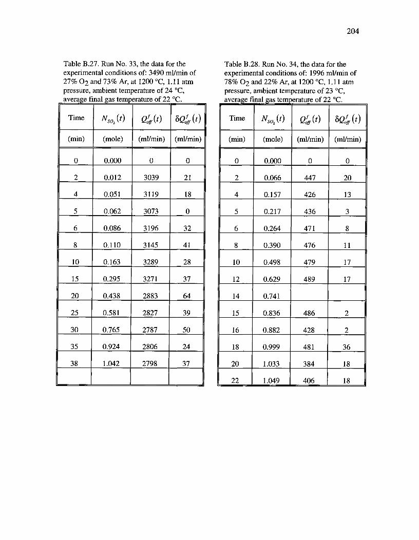
204


Time Ns02 (t) Q.0 fff. (t) 84 (t)


0 0.000 0 0

2 0.012 3039 21

4 0.051 3119 18

5 0.062 3073 0

6 0.086 3196 32

8 0.110 3145 41

10 0.163 3289 28

15 0.295 3271 37

20 0.438 2883 64

25 0.581 2827 39

30 0.765 2787 50

35 0.924 2806 24

38 1.042 2798 37

Table B.28. Run No. 34, the data for theexperimental conditions of: 1996 ml/min of78% 02 and 22% Ar, at 1200 °C, 1.11 atmpressure, ambient temperature of 23 °C,average final as temperature of 22 °C.

Time N0(t) Qcf,ff (t) 84 (t)


0 0.000 0 0

2 0.066 447 20

4 0.157 426 13

5 0.217 436 3

6 0.264 471 8

8 0.390 476 11

10 0.498 479 17

12 0.629 489 17

14 0.741

15 0.836 486 2

16 0.882 428 2

18 0.999 481 36

20 1.033 384 18

22 1.049 406 18

205

Table B.29. Run No. 36, the data for theexperimental conditions of: 2032 rnl/min of22% 02 and 78% Ar, at 1200 °C, 1.08 atmpressure, ambient temperature of 23 °C,average final gas temperature of 22 °C** .

Time Nso, (t) Q(t) 84 (t)


0 0.000 0 0

2 0.012 1735 6

4 0.027 1768 29

5 0.032 1757 12

6 0.041 1724 23

8 0.065 1713 11

10 0.082 1724 32

15 0.148 1717 19

20 0.219 1708 10

25 0.302 1691 21

30 0.391 1711 10

35 0.462 1691 15

40 0.544 1691 7

45 0.629 1696 6

50 0.711 1677 9

55 0.795 1692 7

60 0.882 1688 18

65 0.969 1693 12

Table B.30. Run No. 37, the data for theexperimental conditions of: 2000 ml/min of21% 02 and 79% N2, at 1200 °C, 1.08 atmpressure, ambient temperature of 21 °C,average final gas temperature of 22 °C.

Time Ns02 (t) aofff. (t) 84 (t)(min) (mole) (ml/min) (ml/min)

0 0.000 0 0

2 0.012 1590 32

4 0.024 1616 16

5 0.042 1603 9

6 0.048 1645 0

8 0.060 1639 7

10 0.077 1651 8

15 0.117 1631 23

20 0.198 1635 7

25 0.271 1598 16

30 0.361 1584 23

35 0.451 1608 47

40 0.540 1599 12

45 0.636 1587 12

50 0.713 1582 6

55 0.801 1594 13

60 0.896 1583 17

65 0.990 1597 12

70 1.018 1559 4

** Approximately 77 ml/min argon was used for invoking bath mixing. in this run.


Time Nso, (t) 4(0 84 (t)


0 0.000 0 0

2 0.024 3029 64

4 0.049 3053 13

5 0.067 2971 82

6 0.103 3017 40

8 0.130 2830 10

10 0.167 2933 53

15 0.261 2889 50

20 0.388 2902 110

25 0.545 2938 27

30 0.690 2888 36

35 0.827 2883 43

40 1.001 2839 17

206

Table B.32. The effect of volumetric flow rate of reaction gas on the reaction rates; sample weight of 200 grams of Cu2S; at 1200 °C and 1.08atm; 22% 0 and 78% Ar; lance inside diameter of 3 mm.

Run Q° o P

N so2

0s

N so,0 P

N 02Os

N 02 t *Op

W gaOs

W ga

0 P

W wo^s

W w

(ml/min) (mol/min) (mol/min) (mol/min) (mol/min) (mm) (g/min) (g/min) (g/min) (g/min)9 1480 0.008 0.012 0.011 0.012 25 -0.18 -0.4212 1579 0.009 0.015 2417 1755 0.009 0.013 0.013 0.013 19 -0.16 -0.45 -0.11 -0.2115 2006 0.009 0.016 0.016 0.015 14 -0.07 -0.5736 2032 0.010 0.016 0.015 0.016 14 -0.17 -0.53 -0.14 -0.6621 4055 0.015 0.026 0.023 0.002 11 -0.21 -0.95

Table B.33. The effect of volumetric flow rate of reaction gas on the reaction rates; sample weight of 200 grams of Cu2S; at 1200 °C and 1.08atm; 24% 0 and 76% Ar; lance inside diameter of 3 mm.

Run alOp

Nso2Os

Ns02Op

N 02

o s

N 02 t*0p

W ga0 s

W ga

0 P

W w0 s

Wi,

_ (ml/min) (mol/min) (mol/min) (mol/min) (mol/min) (min) (g/min) (g/min) (g/min) (g/min)8 1010 0.006 0.009 0.009 0.008 36 -0.10 -0.30

41 3516 0.018 0.028 0.025 0.028 13 -0.34 -0.92

207

Table B.34. The effect of reaction gas composition on the reaction rates; sample weight of 200 grams of Cu2S; at 1200 °C and 1.10 atm, 2000ml/min, lance inside diameter of 3 mm.

Run %02Op

Nso2o s

N502Op

N o2o s

N 02 t * Op

W ga

Os

W ga

OP

Ww

0 s

Ww

(mol/min) (mol/min) (mol/min) (mol/min) (min) (g/min) (g/min) (g/min) (g/min)15 22 0.009 0.016 0.016 0.015 14 -0.07 -0.5722 27 0.012 0.021 0.020 0.020 11 -0.15 -0.71 -0.1423 35 0.017 0.027 0.024 0.024 11 -0.28 -0.9424 46 0.027 0.036 0.033 0.036 7 -0.67 -1.15 -1.4225 64 0.037 0.050 0.048 0.050 5 -0.81 -1.6334 78 0.048 0.061 0.063 0.061 5 -1.03 -1.95 -0.85 -2.18

Table B.35. The effect of temperature on the reaction rates; sample weight of 200 grams of Cu2S; at 1200 °C and 1.09 atm, 2000 ml/min of 22%0 and 78% Ar, lance inside diameter of 3 mm.

Run TOp

Ns020 s

N5020p

N o2o^s

N o2 tOp

W ga

Os

W ga

0P

WW

0 sWW

(°C) (mol/min) (mol/min) (mol/min) (mol/min) (min) (g/rnin) (g/min) (g/min) (g/min)15 1200 0.009 0.016 0.016 0.015 14 -0.07 -0.5731 1250 0.012 0.017 0.016 0.017 13 -0.23 -0.57 -0.16 -0.9830 1300 0.013 0.016 0.016 0.016 17 -0.30 -0.53 -0.29 -0.87

208

Table B.36. The effect of temperature on the reaction rates; sample weight of 200 grams of Cu2S; at 1.09 atm, 2000 ml/min of 23% 02 and 77%Ar, lance inside diameter of 3 mm.

Run T. P

N so,

o^s

N so,

. P

NO2Os

NO2 tOp

W ga

o s

W ga

OP

W w

0 s

W

(°C) (mol/min) (mol/min) (mol/min) (mol/min) (min) (g/min) (g/min) (g/min) (g/min)27 1250 0.010 0.016 0.015 0.015 15 -0.19 -0.54 -0.3128 1300 0.012 0.016 0.016 0.016 16 -0.25 -0.49 -0.16 -0.34

Table B.37. The effect of bath mixing on the reaction rates; sample weight of 200 grams of Cu2S; at 1200 °C and 1.09 atm, 2000 ml/min of 22%02 and 78% Ar, lance inside diameter of 3 mm (t appoximate1y 77 ml/min Ar was used to invoke artificial mixing).

Run Q:. P

N so,

o^s

N so,

o P

N 02

Os

N 02

OP

W ga

o s

W ga

0P

W wo s

Ww(nil/min) (mol/min) (mol/min) (mol/min) (mol/min) (min) (g/min) (g/min) (g/min) (g/min)

15 2006 0.009 0.016 0.016 0.015 14 -0.07 -0.5736t 2032 0.010 0.016 0.015 0.016 14 -0.17 -0.53 -0.14 -0.66

Table B.38. The effect of carrier gas type on the reaction rates; sample weight of 200 grams of Cu2S; at 1200 °C and 1.09 atm, 2000 ml/min of21% 0 and 79% Ar, lance inside diameter of 3 mm

Run GasOP

Nso20 s

N so2op

N 0,

0 s

N 0, to P

W ga

0 s

W ga

OP

W iv

0 s

W,„

Type (mol/min) (mol/rnin) (mol/min) (mol/min) (min) (g/min) (g/min) (g/min)_ (g/min)37 Nitrogen 0.008 0.018 0.015 0.016 16 -0.05 -0.61 -0.04 -0.4529 Argon 0.009 0.014 0.013 0.023 22 -0.18 -0.49 -0.08 -0.51

209

Appendix C Reaction Gas Transport Properties

1. Viscosity

The kth approximation of the coefficient of viscosity is given by Equation (C.1), where

the function of 4,(k) is a very slowly varying function of T* and differs only slightly from

unity [109].

266.93 x10-7 1722(21,2)*(T f12(k)L-

Example C.1. This example is to illustrate the procedure for the calculation of the

viscosity of a pure gas. The viscosity of pure argon gas at 1200 °C is calculated as

follows: The molecular weight of argon is MAr = 39.948 g/g.mole. The force constants

for argon are qic= 124°K and a = 3.418A. The reduced temperature is then

T* = KT le = 11.935. The data for the integral S2(2'2)*,for the Lennard-Jones potential

(taken from Hirschfelder et al. [109]) was fitted to a function of the reduced temperature

,as given by Equation (B.2). The value for argon is 0.819. The higher approximation

coefficient, for the viscosity, is fp(k) =1.0073. Substituting for these values in Equation

(C.1), yields gm. = 6.83 x10-4 g/cm.sec.

S2(2'2)* =1.208474/T415703

The viscosity of binary gas mixtures was calculated as follows [110]:

^]]

2

Example C.2. The viscosity of a gas mixture of 20% 02 and 80% Ar, at 1200 °C, is

calculated, Using Equation (C.3), as given by Equation (B.4). The parameters for 02 gas

are the molecular weight of oxygen is M = 31.9988 g/g.mole. The force constants for

210

(C.1)

(C.2)

(C.3)

775

750

725

.i14 7000

.t,".? 675

• ^

mer■ ^ MINAMMINE

6500°

625

600

575

211

oxygen are Eix= 113°K and a = 3.433A. The reduced temperature is then

T* = KT le = 13.035. The higher approximation coefficient is filk) =1.008. Substituting

for these values in Equation (C.1), the viscosity of pure 02, at 1200 °C, is calculated to

be 6.16x10-4 g/cm.sec.

[ 6.84 x10^6.16 x10-40.8^0.2

1-t A r 02 =[/ 1^ + ^= 6.67 x 10-4(g / cm. sec)1/-4^1/

The viscosity of Ar-02 gas mixtures for the temperature range of 1000-1500 °C and at 1

atm is presented below.

550

1000 1050 1100 1150 1200 1250 1300 1350 1400 1450 1500Temperature (°C)

Figure C.1. The viscosity of Ar-02 gas mixtures as a function of temperature, at 1 atm;^ pure Ar;^20% 02, 40% 02; — - — - 60% 02; — - - — 80%02,^ pure 02.

(C.4)

212

2. Diffusion Coefficient

The diffusion coefficients of some selected binary gas mixtures are calculated using

Equation (C.5), as given by equations (C.6-C.10) [1111 The critical properties for these

gases are provided in Table B.1. The results of these calculations were found to compare

very favorably with the measured and calculated results of Hirschfelder et al [109], as

shown in Figure C.2.

DA_B

03

0.43( T )1 81( 1 +

100^1 )

M A MB

( 7' 7' )01405(KA) r

PlOCA,00CB0)^[100)0.4^117c0B0)"

2

Table C.1. The critical properties of some selected gases (taken from Bird et al. [112]).

Gas Tc (°K) Pc (atm) Vc (cm3/mole)

Argon 151 48.0 75.2

Nitrogen 126.2 33.5 90.1

Oxygen 154.4 49.7 74.4

Sulphur Dioxide 430.7 77.8 122.0

0.028565r T 1"1DO —Ar =

2^P^L100

0.0272107 [ TD02-N2=^P^Llooi

(C.5)

1.81

(C.6)

(C.7)

D ^0.020118r T 11 . 81

S02-02 —^P^L100

0.020103 7' -11 81DS02-Ar = P^Lim.]

0.019287 I TDs02-N2^p^Lloo

(C . 1 0)

213

(C.8)

(C.9)

1 00

1 0

oE8')C.)

t,r.4^1a)

CI■1C•11

0•1

z^

0.01

100 1000^

1 0000

Temperature (°K)

Figure C.2. The diffusion coefficients of some selected binary gas mixtures as a functionof temperature, at 1 atm;^ 02-Ar; 0 02-As (after Hirschfelder, calculated); 0 02-Ar (after Hirschfelder, measured); X 02-N2 (after Hirschfelder, calculated); 0 02-N2(after Hirschfelder, measured); — — — 02-S02;^ N2-S02.

PMmix P mix = RT (C.12)

(C.13)Mmix = XAM A+ XBMB•••+XzMz

214

3. Density

Assuming that the gases involved and their mixtures are ideal, the calculation of the gas

density of a pure gas was done via the following equation:

PMAPA =RT (C. 1 1 )

The density of a gas mixture was calculated from Equation (C.12), where the molecular

weight of the gas mixture was calculated using Equation (C.13). The results of these

calculations are shown in Figure C.3.

0.40

0.38

0.36

0.34

0.32to

0.30

'TA 0.28

a 0.26

0.24

0.22

0.205.0

^ I _1(4/ SI I MIRIMINIMIIIMMIliali•ErmINIO,■■

^ IMIN■Ml■AMIIIMMMIMIE%/11111111MINNINE■^ INIMMii•••■Mi•■■••11% IiM1llMPNiill1MIE••O•P'■-^ Ml!?.'dlMlIP"'%IMPCf/I•lM1••lil'■''IMMil-I1•Il_•."d•lIMIMIIr,-^ ...IMMiI•MiMP!r4llMRr/" MCI= MaINIIIMINIMISUMM■^ ...1•1■111■121■-■1•MaIMIPROMPL

AMPERNIP"%■12% MIPTMENIPMWMINPIMINIIP."-_./•■■•••alIMMIIIMMEOMINNEIMIMMIMIM

I•10,--.M.IIIMPISA■1•MaNINIMIIMIMMMIMP/11111=-.■-aNIP%WaINIENNIIMil■MMOMWW■1/1.1111•M

-../..■■■■•••%111/%11•110.3%1M/MMIIMINI■•=1=EMMINOW/M%-■-■•■■■••18■■■■■■1'11•1111"-^111■1•1•M■■allEil■-■11%111•MINI./"/"--a■-■MIMPIMAMIP■IMMPras ..... ■11=MNII,A1•1•%V"-■•■MIN/aMPE21•1%.■ IIIIVAIMPW•ONEall•MMINP/MINN= ..... NMI=MINOMNP!..a1M10--■■■•••■.%•/51•1•2MIIIP///%11■■■■•■• MINII-MIMONN ^IMP/■••■■•■•%..MIEMM

1,•/- I ■"--dMIP/_■""■■■■.1.171.1P.:711:111711111111111111111111111111

1=I=111 1111671T11;;IIMMIIIIIIF^IU

5.5 6.0 6.5 7.0 7.5 8.0

(1/T) x10-4 ( °K-')

Figure C.3. The density of Ar-02 gas mixtures as a function of temperature; for each 10%increments.

Appendix D Temperature Measurements

215

1240

1235 7

1230 —- X x XX XXXXX

xXXXX1225^ X

■-■

(1) 1220 —0 0 0 o 0 0 0 0 0^ 0^0

^

0 0^0tEls,ra,") 1215E0

1ÂAAA

A9210 A^

AAAEli)A^

AÂÂ

1205 - 000U 0 aoao X o o

1200 -/)-DO^ X^00

1195

0 50 100

Time (min)

150 200

Figure D.1. The manual temperature measurement of the center of the melt; 200 gramsCu2S, at 1200 °C, E Run No. 5. (922 ml/min of 26%02 and 74% Ar); 0 Run No.7 (922ml/min of 26%02 and 74% Ar); A Run No. 8 (1010 ml/min of 24%02 and 76% Ar); 0Run No. 9. (1546 of 24%02 and 76% Ar); x Run No. 15. (2006 mllmin of 22%02 and78% Ar); + Run No. 16. (2510 ml/min of 23%02 and 77% Ar).

AA

t +

f +

0

I I^'^'11 ,Ill!L I ILI,_, , p I

1200 -D-a

1195

---000000^0^0^0

00^ 00^0

0^00^0_-_.0^

000^0^0^0

--0

-__0

0^0^0^00 0^0^0^0^0

0^0

1240

1235

1230

;7.(`).-1

1225

0 1220

—

—

-0-

1205 --:0

0^10^20^30^40^50^60^70^80

Time (min)

Figure D.2. The manual temperature measurement of the gas at the same height of thelance nozzle; 200 grams Cu2S, at 1200 °C, III Run No. 18. (2234 ml/min of 23%02 and77% Ar); 0. Run No. 22. (1998 mllmin of 27%02 and 73% Ar); 0 Run No. 19. (3015 of23%02 and 77% Ar).

216

217

^

1210 ^

1208 -P'--' 1206 -2=ci 1204 -t,s=1

^

0 1202 ^4

1200 -

^

1198 ^0 10^20^30^40^50^60^70

Time (min)

Figure D.3. The gas temperature measurement at the same height of the lance nozzle forRun No. 27, the experimental conditions of 200 grams Cu2S, at 1200 °C, 1998 ml/min of27% 02 and 73% Ar.

^

1288 - ^1286 -

a 1284 -

c`---' 1282

§ 1280t 12781.1 1276

E-41274 -1272 -

1270 0 10^20^30^40^50^60^70^80

Time (min)

P^,

i^ 1i ) 6

Figure D.4. The temperature measurement at the center of the melt for Run No. 29, theexperimental conditions of 200 grams Cu2S, at 1275 °C, 1994 ml/min of 23% 02 and77% Ar.

1330

218

/

/

1325

P\'..-- 13200.)6-'vd 1315 _atsa.0 1310

E-41305

f13000

.^1^.10^20^30^40^50^60^70^80

Time (min)

I

1i

, /


1235

1230

P 1225.....,a) 1220

+6:16-41-, 1215P.°1) 1210E-1

1205

1200

0^5^10^15^20^25^30^35^40

Time (min)


219

1270 ^

1260 7

E6.3 1250 7

2). 1240 -=

9.,(1) 1230 7

E-1 1220 7

1210 -

1200 ^0

Time (min)


5^10^

15 20 25

1218

1216

1214

1212.)

AR' 1210

1208

1206

1204

12020^10^20^30^40^50^60^70

Time (min)

Figure D.8. The gas temperature measurement at the same height of the lance nozzle forRun No. 37, for the experimental conditions of 200 grams of Cu2S at 1200 °C, 2000ml/min of 21% 02 and 79% N2.

220

Figure D.9. The gas temperature measurement at the same height of the lance nozzle forRun No. 41, for the experimental conditions of 200 grams of Cu2S at 1200 °C, 3500ml/min of 24% 02 and 76% Ar.

oxidation kinetics of molten copper sulphide

Documents