oxygen binding thermodynamics of human hemoglobin in the

University of Nebraska - Lincoln University of Nebraska - Lincoln

DigitalCommons@University of Nebraska - Lincoln DigitalCommons@University of Nebraska - Lincoln

Student Research Projects, Dissertations, and Theses - Chemistry Department Chemistry, Department of

Spring 3-2021

Oxygen Binding Thermodynamics of Human Hemoglobin in the Oxygen Binding Thermodynamics of Human Hemoglobin in the

Red Blood Cell Red Blood Cell

Kyle K. Hill University of Nebraska-Lincoln, [email protected]

Follow this and additional works at: https://digitalcommons.unl.edu/chemistrydiss

Part of the Analytical Chemistry Commons, and the Physical Chemistry Commons

Hill, Kyle K., "Oxygen Binding Thermodynamics of Human Hemoglobin in the Red Blood Cell" (2021). Student Research Projects, Dissertations, and Theses - Chemistry Department. 106. https://digitalcommons.unl.edu/chemistrydiss/106

This Article is brought to you for free and open access by the Chemistry, Department of at DigitalCommons@University of Nebraska - Lincoln. It has been accepted for inclusion in Student Research Projects, Dissertations, and Theses - Chemistry Department by an authorized administrator of DigitalCommons@University of Nebraska - Lincoln.

https://digitalcommons.unl.edu/

https://digitalcommons.unl.edu/chemistrydiss

https://digitalcommons.unl.edu/chemistrydiss

https://digitalcommons.unl.edu/chemistry

https://digitalcommons.unl.edu/chemistrydiss?utm_source=digitalcommons.unl.edu%2Fchemistrydiss%2F106&utm_medium=PDF&utm_campaign=PDFCoverPages

http://network.bepress.com/hgg/discipline/132?utm_source=digitalcommons.unl.edu%2Fchemistrydiss%2F106&utm_medium=PDF&utm_campaign=PDFCoverPages

http://network.bepress.com/hgg/discipline/139?utm_source=digitalcommons.unl.edu%2Fchemistrydiss%2F106&utm_medium=PDF&utm_campaign=PDFCoverPages

https://digitalcommons.unl.edu/chemistrydiss/106?utm_source=digitalcommons.unl.edu%2Fchemistrydiss%2F106&utm_medium=PDF&utm_campaign=PDFCoverPages

OXYGEN BINDING THERMODYNAMICS OF HUMAN HEMOGLOBIN

IN THE RED BLOOD CELL

by

Kyle Kelly Hill

A DISSERTATION

Presented to the Faculty of

The Graduate College at the University of Nebraska

In Partial Fulfillment of Requirements

For the Degree of Doctor of Philosophy

Major: Chemistry

Under the Supervision of Professor Mark Griep & Professor Lawrence Parkhurst

Lincoln, Nebraska

March 2021

OXYGEN BINDING THERMODYNAMICS OF HUMAN HEMOGLOBIN

IN THE RED BLOOD CELL

Kyle Kelly Hill, Ph.D.

University of Nebraska, 2021

Advisors: Lawrence J. Parkhurst & Mark Griep

We report for the first time the binding constants and Hill numbers for oxygen in the red

blood cell under physiological conditions. When compared to our results for hemoglobin

in solution, our results show conclusively that hemoglobin binds oxygen more tightly and

with lower co-operativity when packed in the red blood cell. At 18°C, these differences

are striking: the respective half-saturation values are 15.57 µM (in red blood cells) and

18.83 µM (in solution), with corresponding Hill numbers of 2.475 (in red blood cells) and

2.949 (in solution). The optical complications that arise from high turbidity of red blood

cell suspensions have been overcome via instrumental and analytical innovations. First, a

modified internal cavity absorption meter (ICAM) using a suspension of strongly

scattering milk particles yielded long optical path lengths, amplifying the target signal.

Second, the detection of oxygen binding from 600 to 670 nm eliminated the multiple

unwanted wavelength dependences of apparent fractional saturation found in the

conventional 535 to 580 nm range. Finally, a transfer function made it possible to extract

all thermodynamics data from the scattered light. Since the hemoglobin tetramer expands

when it releases oxygen, our work suggests that dense packing of hemoglobin in the RBC

must constrain this molecular expansion. The higher oxygen affinity and lower co-

operativity results in a substantially more distributed delivery of oxygen into diverse

body tissues, such as the lungs and the brain. Furthermore, consequent thermodynamic

studies suggest that the differences arise mostly from an entropy difference between

hemoglobin in the red blood cell and hemoglobin free in solution. All of these results

contrast sharply with the decades-long assumption that the behavior of hemoglobin free

in solution is an appropriate model for understanding the physiology of oxygen binding

and delivery, and that those curves are physiologically relevant.

Acknowledgements

To my parents

Who never lost vision

To Denise

whose love, patience, and support cannot be described in words, but I try anyway

To Dr. Parkhurst & Dr. Griep

Without their support this research would have never been undertaken nor written

Table of Contents

1. Introduction to Hemoglobin ........................................................................................ 1

1.1 Hemoglobin Conformational Changes ..................................................................2

1.2 Hemoglobin Disease States ...................................................................................4

1.3 History of Hemoglobin Oxygen-Binding Research ..............................................9

1.4 Chemical Environment of Red Blood Cells ........................................................10

2. Integrated Cavity Absorption Meter: Design & Validation ...................................... 14

2.1 Introduction .........................................................................................................14

2.2 Materials and Methods ........................................................................................17

2.3 Results .................................................................................................................30

2.4 Discussion ...........................................................................................................41

3. Oxygen-Binding of Hemoglobin in Solution Compared to Hemoglobin within the Red Blood Cells at 18°C ................................................................................................... 46

3.1 Introduction .........................................................................................................46


3.3 Results .................................................................................................................53

3.4 Discussion ...........................................................................................................59

4. Comparison of Thermodynamics of Oxygen-Binding of Hemoglobin in Solution versus Hemoglobin in the Red Blood Cell ....................................................................... 64

4.1 Introduction .........................................................................................................64


4.3 Results .................................................................................................................67

4.4 Discussion ...........................................................................................................76

5. Appendix ................................................................................................................... 79

5.1 MWC Oxygen-Binding Thermodynamic Parameters .........................................79

5.2 Wavelength Dependent Effects ...........................................................................81

5.3 Buffers and the Intracellular Chemical Environment of the Red Blood Cell .....81

5.4 HBRBC Oxygen-Binding Thermodynamics Assuming No Cooperativity ...........82

5.5 Red Blood Cell Storage, Retrieval, and Survival ................................................85

5.6 Dissolved Oxygen Concentration........................................................................89

5.7 Determination of the Transfer Function Equation ..............................................90

6. Bibliography ............................................................................................................. 92

Table of Figures

Figure 1.1: Molecular Lung in Reverse: Hemoglobin ........................................................ 8

Figure 1.2: Center-to-Center Distances for Hemoglobin in Solution Compared to in Red

Blood Cells........................................................................................................................ 13

Figure 2.1: Light Path through the ICAM ........................................................................ 21

Figure 2.2: Instrumentation to Measure Oxygen-Binding Thermodynamics of

Hemoglobin....................................................................................................................... 22

Figure 2.3: Flow of Water-Saturated Nitrogen Gas into the Air Space Led to Gentle

Deoxygenation of the Solution ......................................................................................... 25

Figure 2.4: Instrumentation to Measure Oxygen-Binding Thermodynamics of

Hemoglobin....................................................................................................................... 26

Figure 2.5: Relating Molar Absorptivity to Molar ICAM Absorptivity ........................... 33

Figure 2.6: Transformed ICAM Absorbance Overcomes Light Scattering ...................... 35

Figure 2.7: Myoglobin Oxygen-Binding Thermodynamics ............................................. 40

Figure 2.8: The Spectrum of Oxygenated Hemoglobin at Two Different Concentrations45

Figure 3.1: Oxygen-Binding Thermodynamics of Hemoglobin Determined by The

Relationship between Absorbance and Oxygen Concentration ........................................ 52

Figure 3.2: Determining the Fractional Saturation from Absorbance and Oxygen

Concentration .................................................................................................................... 56

Figure 3.3: Hemoglobin Oxygen-Binding Compared to Literature .................................. 60

Figure 3.4: Difference of Hemoglobin Oxygen-Binding in Different Environments ...... 61

Figure 4.1: Oxygen-Binding Curves of HBRBC at Different Temperatures ...................... 70

Figure 4.2: Oxygen Binding Curves of Hemoglobin in Solution ..................................... 71

Figure 4.3: Van’t Hoff Plots for KT .................................................................................. 73

Figure 5.1: Oxygen-Binding Curves of HBRBC at Varying Temperatures Assuming No

Cooperativity..................................................................................................................... 83

Table of Tables

Table 1.1: Examples of Hemoglobin Thalassemiasa .......................................................... 7

Table 2.1: Parameters & Fits of ICAM Spectrophotometry ............................................. 31

Table 3.1: Hemoglobin Oxygen-Binding Parameters in Solution and in the RBC (18°C)

........................................................................................................................................... 57

Table 4.1: Oxygen-Binding Thermodynamic Parameters ................................................ 75

Table 5.1: MWC Parameters of Hemoglobin in Solution ................................................. 80

Table 5.2: MWC Parameters of Hemoglobin in the Red Blood Cell ............................... 80

Table 5.3: Oxygen Binding Thermodynamics of HBRBC Assuming Dimer

Thermodynamics............................................................................................................... 84

Table of Equations

Equation 2.1: Transfer Function……………………………………………………… Equation 2.2: Inverse Transfer Function……………………………………………... Equation 2.3: Myoglobin Oxygen-Binding Equilibrium……………………………... Equation 2.4: Fractional Saturation Defined by A0, Aꝏ, and ACOLL ………………….. Equation 2.5: Myoglobin Oxygen-Binding Equilibrium and Fractional Saturation…. Equation 2.6: Definition of A0 as Myoglobin Fractional Saturation…………………. Equation 2.7: A0 Defined as Myoglobin Fractional Saturation Extrapolation………... Equation 2.8: Reciprocal of Myoglobin Oxygen-Binding Equilibrium and Fractional Saturation……………………………………………………………………………... Equation 2.9: Definition of Aꝏ as Myoglobin Fractional Saturation…………………. Equation 2.10: Aꝏ Defined as Myoglobin Fractional Saturation Extrapolation……… Equation 2.11: Fractional Saturation Defined by A0, Aꝏ, and ACOLL………….……… Equation 2.12: Myoglobin Oxygen-Binding Equilibrium…..………………………... Equation 3.1: Adair Oxygen-Binding Polynomial………..………………………….. Equation 3.2: MWC Hemoglobin Oxygen-Binding Polynomial…………………….. Equation 3.3: Hill Equation…………………………………………………………... Equation 3.4: Fractional Saturation Defined by A0, Aꝏ, and ACOLL………................... Equation 3.5: Adair Oxygen-Binding Polynomial and Fractional Saturation………... Equation 3.6: Definition of A0 as Hemoglobin Fractional Saturation……………….. Equation 3.7: A0 Defined as Hemoglobin Fractional Saturation Extrapolation……… Equation 3.8: Reciprocal of Hemoglobin Fractional Saturation…………….……….. Equation 3.9: Definition of Aꝏ as Hemoglobin Fractional Saturation………………..

32 32 36 36 37 37 37 37 37 38 38 38 47 49 50 53 54 54 54 55 55

Equation 3.10: Aꝏ Defined as Hemoglobin Fractional Saturation Extrapolation……………………………………………………………………...…... Equation 3.11: Simplification of Aꝏ Defined as Hemoglobin Fractional Saturation Extrapolation……......................................................................................................... Equation 4.1: Gibbs Free Energy with Equilibrium Constant………………………... Equation 4.2: Gibbs Free Energy Equation…………………………………………... Equation 4.3: Derivation of the van’t Hoff Equation………………………………… Equation 4.4: van’t Hoff Equation Defined with Two Equilibrium Constants………. Equation 4.5: van’t Hoff Equation…………………………………………………… Equation 5.1 Hemoglobin Dimer Oxygen-Binding Equilibrium…………………….. Equation 5.2: Lab Air Pressure Equation…………………………………………….. Equation 5.3: Oxygen Activity Equation…………………………………………….. Equation 5.4: Overall ICAM Intensity………………………………...……………... Equation 5.5: Oxygenated Hemoglobin Intensity in the ICAM…...…………………. Equation 5.6: Deoxygenated Hemoglobin Intensity in the ICAM…………………… Equation 5.7: Fractional Saturation of Hemoglobin Based on ICAM Intensity……...

55 55 64 65 65 65 65 82 89 89 90 91 91 91

1

1. Introduction to Hemoglobin

Physiology of Human Hemoglobin

In the human body, hemoglobin serves several major functions, the most

important function is delivery of oxygen from the lungs to the tissues. The smallest

branches of the lungs are called alveoli, an environment with high oxygen concentration.

Gas exchange occurs in the alveoli, where carbon dioxide passes from the blood to the

lungs. Oxygen binds to the hemoglobin in the red blood cell. After passing through the

heart, the red blood cells travel through the vascular system deliver oxygen to the tissues.

The oxygen unloaded from hemoglobin travels by diffusion to myoglobin, which has a

higher affinity toward oxygen than hemoglobin. Finally, the oxygen travels to

cytochrome oxidase in the electron transfer system, which has a higher oxygen affinity

than myoglobin. Hemoglobin α and β subunits have very similar structures, and both are

similar to myoglobin. However, hemoglobin is a remarkably efficient oxygen carrier and

is able to use up to ninety percent of its potential oxygen-carrying capacity efficiently.

Under similar physiological conditions, myoglobin would be able to use only seven

percent of its potential oxygen-carrying capacity. Myoglobin exists as a monomer and

functional hemoglobin is a tetramer. The tetramer structure allows hemoglobin to bind

oxygen cooperatively, meaning that the binding of oxygen to a single heme increases the

likelihood that the remaining chains will bind oxygen. This is due to the allostery of

hemoglobin. The conformation of hemoglobin changes from the oxygenated state to the

deoxygenated state, depending upon the ligands bound to the hemoglobin. The presence

of bound oxygen changes changing both the tertiary and quaternary structure of

hemoglobin.

2

1.1 Hemoglobin Conformational Changes

Hemoglobin is vital to life, as it transports oxygen from the lungs to the tissues

and helps with the transport of carbon dioxide from the tissues to the lungs. The binding

affinity increases during the stepwise binding of four oxygen molecules leading to a

sigmoidal binding curve. Since the beginning of the century hemoglobin has attracted

numerous investigations because of its interesting physiologically and physical

interactions with ligands. Although the structure and function of hemoglobin has been

investigated more extensively than all other allosteric proteins, the molecular mechanism

of its action is still unclear.

For over one hundred years, it has been known that hemoglobin crystalizes in two

distinct states depending on the degree of oxygenation. In 1893, deoxygenated

hemoglobin crystals were observed to shatter when exposed to oxygen, suggesting that

hemoglobin changed in size during oxygenation.1,2 Further evidence of the two states

came from x-ray crystallography in 1959 and in 1963, when Perutz elucidated the

structure of oxygenated hemoglobin and deoxygenated hemoglobin, respectively.3,4 Each

of the two α- and two β-globins contain a heme ring: a porphyrin with one central Fe

atom that can bind and release one oxygen molecule. In oxygenated hemoglobin

conformation, the heme lies in an isolated pocket where it is tightly wedged between the

16 side chains of the globin. This constrains the iron to lie within the plane of the

porphyrin ring. The iron is hexacoordinate with four bonds to the porphyrin ring, one

bond to histidine, and the sixth to the oxygen. In the deoxygenated conformation, the

iron is in a 5-coordinated form, losing the interaction with oxygen. The iron becomes

displaced from the porphyrin plane by 0.4 Å.5 The distal valine obstructs the

3

deoxygenated conformation on the ligation side and this obstruction cannot be cleared

without a change in the polypeptide structure. Within these two different conformations,

the globins determine the relationship of the iron within the porphyrin ring. As pointed

out by Perutz and others, the dominant structural change between all four globins can be

described as the α1β1 and α2β2 dimers remaining rigid while the contacts between α1β2,

α2β1, α1α2, and β1β2 move relative to each other.6 During deoxygenation, the α1α2, α1β1,

and α2β2 heme distances remain stationary while the α1β1 and α2β2 act as hinges. Most

notably, the β1β2 heme distance increases 5Å (fig. 1.1). This led Perutz to describe

hemoglobin functioning as a "molecular lung in reverse," contracting as it binds oxygen

and expanding as it releases oxygen.7

Tertiary Structural Changes Upon Oxygenation

The changes in the tertiary structure of hemoglobin are small in scale compared to

those of the quaternary structure, but the changes in the tertiary structure induce the

quaternary structural changes. The displacement of the iron atom gives rise to movement

of the proximal histidine. This causes the associated alpha helix to move toward the

heme plane. This movement is propagated to other helices, and further amplified toward

the carboxyl termini of the hemoglobin monomer. In deoxyhemoglobin, two tyrosine

side chains occupy pockets between two helices. The tyrosine hydroxyl groups are

hydrogen-bonded to the carbonyl groups of two valines. Upon oxygenation, the tyrosine

side chains are expelled from the pockets, giving rise to the rupture of salt bridges

involving carboxyl terminal residues. Upon expulsion of the tyrosine side chains, the

thiol group of a cysteine moves into the tyrosine pocket, which is competed for by these

4

two side chains. The rupture of the salt bridges in the carboxyl terminal region causes the

further rupture or weakening of other salt bridges.

Quaternary Structural Changes Upon Oxygenation

The binding of oxygen to one hemoglobin subunit is accompanied by a complete

rearrangement of the four monomers. From the perspective of an α1 monomer, α2 is turns

16° and shifts by 2.1 Å, β1 by 3.7° and 1.9 Å, and β2 by 13.5° and 1.9 Å. Upon this

transition, the symmetry is preserved but a new axis replaces the previous. There is no

significant conformational change at the α1-β1 contact, but the α1-β2 contact region

undergoes significant changes. The monomers shift by 6 Å, resulting in a change in the

number, type and combination of the amino acid chain interactions. The amino acid

residues involved in the bonds or contacts with the heme group, in the α1-β2 contact

region, are all important for the physiological functioning of hemoglobin, and almost all

of them are ubiquitous.

1.2 Hemoglobin Disease States

Numerous disease states of hemoglobin exist. They are caused by abnormal

levels of hemoglobin monomers or the expression of abnormal hemoglobins. The

majority of hemoglobin in human adults is hemoglobin A, a tetramer consisting of two α-

and two β-globins. Although its physiological role is unclear, 1-3% of all human

hemoglobin tetramers exist as two α-globins and two δ-globins, hemoglobin A2. During

fetal development, humans produce hemoglobin F consisting of two α- and two γ-

globins. Hemoglobin F has a higher oxygen affinity than hemoglobin A. After birth,

most of the γ-globins are replaced by β-globins with the result that 1-4% of hemoglobin

in the average adult human is hemoglobin F.

5

Many hemoglobin variants can be expressed (Table 1.1). The most common

abnormal hemoglobin expressed is the s-globin, the cause of sickle cell anemia.8 The s-

globin gene is autosomal recessive, replacing the β-globin gene. When both inherited

genes express the s-globin, sickle cell anemia occurs. When one inherited gene expresses

s-globin and the other expresses β-globin, the individual’s oxygen transport system is not

much effected but they experience fewer effects during malarial infections. This led to

evolutionary selection for the gene in malaria-stricken portions of the world.9 Carriers

will only show symptoms under very low oxygen concentration, or when dehydrated.

Sickle cell disease can be devasting for humans with the double recessive gene.

While the symptoms can vary from person to person, the major effects are anemia,

bacterial infections, swelling of the hands and feet, and stroke. Humans with the disease

can experience a sickle cell crisis, including vaso-occlusion and hemolysis of the red

blood cells lasting roughly a week.10 This crisis can be brought about by infection,

dehydration, or acidosis, but no predisposing cause has yet to be identified.11 The life

expectancy of sickle cell disease patients is 30-60 years in countries with modern

medicine.12

The sickle cell disease state was the first genetic disease identified.13 The s-

globin gene is a single nucleotide mutation in the β-globin gene, exchanging a guanine-

adenosine-guanine codon for a guanine-thymine-guanine codon. The β-globin glutamine

at position 6 is replaced with valine. The hemoglobin S structure does not differ

substantially from hemoglobin A, and in dilute solution both have physiologically similar

oxygen-binding thermodynamics.14,15 However, at high hemoglobin concentration in the

6

red blood cell, low oxygen concentration brings about sickling of the red blood cell when

the hemoglobin polymerizes due to an exposed hydrophobic portion of the tetramer.16

The sickling occurs most drastically in deoxygenated blood and is most problematic in

the capillaries. Thus, the disease state requires the concentrated hemoglobin environment

that occurs within the red blood cell. The majority of robust hemoglobin oxygen-binding

equilibrium studies were done in dilute solution. In contrast, studies of the

thermodynamics of hemoglobin oxygen-binding within the red blood cell are limited.

We sought to develop novel robust experimentation to compare hemoglobin oxygen-

binding thermodynamics within the red blood cell to hemoglobin free in dilute solution.

7

Table 1.1: Examples of Hemoglobin Thalassemiasa

Hemoglobin Thalassemia

Expression Pathology

HbS/HbC8 HbB mutation: E6K

Sickling of deoxygenated RBCs, anemia, poor circulation, early death

HbE17,18 HbB mutation: E26K

Growth retardation, splenomegaly, hepatomegaly, jaundice, bone abnormalities, and cardiovascular problems, early death

Hb Bart’s19 Hbγ is overexpressed and replaces HbA

Tetramers of 4 fetal hemoglobins are insoluble and accumulate in the RBC

Death shortly after birth without blood transfusions

Hb D-Punjab20

HbB single-point mutation

Heterozygous: asymptomatic Homozygous: mild anemia and slight

splenomegaly Hb O Arab21 HbB single-point

mutation: E121K

Heterozygous: mild sickling of deoxygenated red blood cells, rare anemia

Homozygous: major sickling of deoxygenated RBCs, anemia, poor circulation

Hb O-Padvoa

HbB single point mutation: E11K

Heterozygous: asymptomatic Homozygous: severe anemia, splenomegaly,

abnormal RBC Hb O-

Indonesia22 HbB single-point

mutation: E116K Asymptomatic

Hb H23 Impaired production of 3 of 4 α-globins

Hemolytic anemia, splenomegaly, hepatomegaly, jaundice, bone deformities

Hb Lepore24 Fusion of HbB and HbD gene loci. Hemoglobin consists of 2 α-globins and 2β/δ-globins

Heterozygous: Asymptomatic Homozygous: Severe anemia, splenomegaly,

hepatomegaly, bone deformities

Hb M HbB single-point mutation: K67E

Heterozygous: 15-30% levels of methemoglobin in the RBC

Hb Kansas25 HbB single-point mutation: N102T

Heterozygous: raised levels of methemoglobin in the RBC

aMany thalassemias of hemoglobin exist. The majority of them are pathologically recessive and are single-point mutations in the HbB gene, changing a hydrophilic amino acid to a hydrophobic residue on the tetramer's outer surface. These cause misshapen red blood cells upon deoxygenation, leading to enlargement of the spleen and liver, bone deformities, and anemia. Some single-point mutation exchange a hydrophobic residue for a hydrophilic amino acid in the interior of the tetramer, causing high populations of methemoglobin formation. The major focus of thalassemia study is pathological on patient symptoms and genetic causes, with limited studies of the oxygen-binding equilibria inside and outside of the red blood cells.

8

Figure 1.1: Molecular Lung in Reverse: Hemoglobin

The distance between the oxyhemoglobin β1Fe- β2Fe hemes is 34.6 Å (solid red), which expands to 39.6 Å in the deoxyhemoglobin conformation (solid blue). This relates to a volume expansion of 15%.

9

1.3 History of Hemoglobin Oxygen-Binding Research

Hemoglobin has been a model protein for the scientific community for the past

two hundred years. Hemoglobin is easy to obtain, and the color makes it easy to work

with in the lab. In 1825, Engelhart showed that the iron-to-protein ratio in hemoglobin

was similar across multiple species.26 In 1878, Bert obtained the first crude hemoglobin

oxygen-binding measurements using gasometric methods.27 Using similar techniques,

Bohr found that pH changed the equilibrium of hemoglobin oxygen-binding.28

Subsequent studies concluded that other molecule concentrations, such as salt and

diphosphoglycerate, drastically altered the hemoglobin oxygen-binding equilibrium.

These molecules regulated the hemoglobin oxygen-binding thermodynamics by binding

to a site other than the active site and were called allosteric effectors. Further gasometric

methods developed by Barcroft and Haldane were used to study hemoglobin oxygen-

binding equilibrium.29,30 These gasometric measurements often utilized a Van Slyke

apparatus.31 The Van Slyke apparatus uses a round-bottom flask filled with a solution of

deoxygenated hemoglobin. A measured amount of air with oxygen is introduced to the

flask and given time to equilibrate. A small drop in the pressure indicated the binding of

oxygen to hemoglobin. These experiments could be used to study hemoglobin oxygen-

binding within the red blood cell. However, even recent automated gasometric

measurements take considerable amounts of time and are prone to measurement errors.32

Later, spectrophometric techniques provided more precise data, allowed for

multiple measurements per sample, and required much less protein. As a result,

spectrophotometric methods have largely replaced the gasometric methods. Imai, often

considered Adair’s protégé, worked extensively on the ligand-binding properties of

10

hemoglobin. In the 1970s and 1980s, Imai et. al. developed a method to study the

functional properties of abnormal hemoglobin, and later improved this method to

determine the oxygen-hemoglobin equilibrium curves. The Imai method uses the

absorbance changes of hemoglobin at a single wavelength to determine the oxygen

saturation and uses an oxygen electrode to determine the oxygen concentration. A

solution of oxyhemoglobin was placed into a cell with magnetic stirring, and this cell is

in the beam of a double-beam spectrophotometer with the path length ranging from 5 to

25 mm. The temperature is controlled by water circulating around the cell. A small

thermistor is placed within the cell to measure the temperature of the sample. The gas

phase above the liquid was filled and continuously replaced with argon or nitrogen, and

the dissolved oxygen was removed from the solution. The percent of heme bound with

oxygen, or fractional saturation, was measured utilizing Beer’s law. The fractional

saturations were compared to the solution's oxygen concentration. These measurements

allowed for greater resolution, but a considerable problem arose. Spectrophotometric

measurements within the red blood cells were limited as the scattered light from the

turbid solution created too much signal-to-noise. Most spectrophotometric hemoglobin

oxygen-binding studies used free hemoglobin. Most spectrophotometric measurements of

hemoglobin oxygen-binding utilized a hemoglobin concentration of 100 µM to ensure the

tetramer does not dissociate to dimers.33 This is 200-fold less concentrated than in the

cell.

1.4 Chemical Environment of Red Blood Cells

For most vertebrates, hemoglobin delivers oxygen from the lungs or gills to the

tissues. If the protein was used in solution to provide oxygen, then two critical

11

difficulties arise. First, the iron in the hemoglobin is toxic.34 Second, adequate oxygen

delivery from the lungs to the tissues would require a viscous solution, putting an

incredible strain on the heart.35,36 The red blood cell eliminates the iron toxicity by

containing the iron within a cell membrane and increases oxygen delivery rates by

maximizing the surface area to volume ratio by adopting a biconcave disc shape. The red

blood cells are roughly 90 fL and can expand freely to 150 fL.37,38

The capillaries are half the diameter of the red blood cell, so the cells bend and

contort to fit through the capillaries one cell length apart.39–42 The cigar shape increases

the surface area interaction of the red blood cell with the capillary, thus increasing the

rate of gas exchange to the surrounding tissues. The elasticity of the red blood cell

membrane is maintained by membrane proteins, such as band 3 protein and others. In the

arteries and isotonic solutions, the red blood cell has a diameter of 6-8 µm and a

thickness of 2 µm.

The red blood cell has a hemoglobin tetramer concentration of 5 mM, which gives

an average tetramer center-to-center distance of 76 Å, as contrasted to 280 Å for most

spectrophotometric measurements (fig. 1.2). In fact, the interior of the red blood cell has

30-40% less water due to the high concentration of hemoglobin and other proteins. It

was our hypothesis that this crowded environment plays a major role in hemoglobin

oxygen-binding because there are more protein-protein interactions. To test this

hypothesis, we used an integrated cavity absorption meter spectrophotometer with novel

correcting functions to determine the oxygen-binding thermodynamics of hemoglobin in

12

the red blood cell. Then, we contrasted those results with the findings with hemoglobin

in solution.

13

Figure 1.2: Center-to-Center Distances for Hemoglobin in Solution Compared to in Red Blood Cells

The typical spectrophotometric experimentation of hemoglobin deoxygenation utilizes hemoglobin concentrations of 100-150 µM, which is a center-to-center tetramer distance of 280 Å (A, B).32,43,44 The hemoglobin concentration in the RBC ranges from 4810-5580 µM as a tetramer in the RBC (C,D).45 In the RBC, the tetramer center-to-center distance is 76 Å from literature (sphere estimation). For standard spectrophotometric experimentation, the high concentration of the hemoglobin in the RBC combined with the light scattering effect of the RBC in solution prevents spectral measurements. Due to proximity with other tetramers, we predicted the crowding affects the oxygen-binding thermodynamics of the hemoglobin.

14

2. Integrated Cavity Absorption Meter: Design & Validation

2.1 Introduction

Purpose of ICAM Spectrophotometry

In most previous spectrophotometric studies of hemoglobin oxygen-binding

equilibria, the measurements were taking using translucent solutions of dilute protein. At

visible wavelengths, the wavelength of light is much larger than the diameter of

hemoglobin at 5 nm, and the sample does not scatter light. The average solution of

hemoglobin used in spectrophotometric measurements at 100 µM (tetrameric

concentration) is translucent. This concentration is high enough to overwhelm the

tetramer/dimer dissociation (Kd = 1 µM, under standard conditions), but low enough to

not overwhelm the signal-to-noise of the spectrophotometer.46 In contrast, a solution of

red blood cells is turbid. Human red blood cells are larger than the amplitude of light,

leading to light scattering and a significant signal-to-noise loss.47 The scattering effects

have always been a systematic problem in absorption measurements, and there have been

multiple attempts to correct for this scattering.48 One of these attempts is the Integrating

Cavity Absorption Meter or ICAM.

Basic Physical Description of ICAM Setups

The ICAM spectrophotometer utilizes a round-bottom flask with an entrance and exit

window, with either the inner or outer diameter of the sphere coated with a highly diffuse

reflecting white material (fig. 2.1). The walls reflect scattered light until the sample

absorbs the photons or the light leaves through either of the windows.49 The

photomultiplier collects the light leaving the exit window. Afterward, the

15

photomultiplier contrasts the light energy from the sample to a blank. For instance,

ICAMs are used in studies of pollution detection or sea particles with low extinction

coefficients and low concentrations.50,51 The biggest drawback of ICAM

spectrophotometers is that absorbances do not relate linearly with concentration and do

not reflect Beer's law. Nevertheless, over 70 years of theoretical and experimental

research has resulted in methods to correlate ICAM absorbance measurements with the

absorbance readings gathered from a spectrophotometer utilizing collimated light.

History of Relating ICAM Absorbances to Collimated Absorbances

Initial work on an ICAM began in 1953 when Walsh proposed that, if the light is

introduced through a small entrance window and the sphere's surface was Lambertian

reflective, then any point of reflectance in the ICAM will illuminate all other surfaces of

the wall equally.52 In 1970, Elterman continued the work by devising an integrating

cavity and deriving the absorbance coefficients based upon the measured absorbances.53

The calculations assumed that the energy of light at all points of the walls being equal. In

1992, Fry continued his work and corrected Elterman's derivations.54,55 The derivations

use an average pathlength in the ICAM, derived from using the photon energy of the light

being equal at any one point of the ICAM. Parkhurst developed the correct equations for

both spherical and cubic ICAM to obtain absorbance coefficients from measured

absorbance of the ICAM by considering the precise distribution of path lengths (see

appendix 5.7). Instead of treating the ICAM with average energy, Parkhurst integrated

over the probabilities of all pathlengths within the ICAM. Using these results, Parkhurst

found that relating the ICAM measured absorbance to absorbance per centimeter would

16

follow an exponential complement. With the corrections, it became possible for us to use

ICAM measurements to determine the percent of hemoglobin oxygen-binding sites bound

in a way that is directly proportional to concentration.

Overview of ICAM Spectrophotometry Validation

The determination of hemoglobin oxygen-binding thermodynamics requires

measuring both the percent of hemoglobin oxygen-binding sites bound and oxygen

concentration in solution. In our case, the ICAM absorbance measurements determined

the percent of hemoglobin oxygen-binding sites bound, while a Clark oxygen electrode

determined the solution's oxygen concentration.56,57 Our initial ICAM experiments had a

three-fold purpose. First, we tested Parkhurst’s derivations by determining a transfer

function. The transfer function corrected ICAM scattered light absorbance to an

equivalent collimated absorbance per centimeter. Second, we tested the transfer function

by comparing the corrected ICAM measurements to measurements gathered by a

collimated spectrophotometer using samples that scatter light with those that do not.

Third, both the oxygen electrode and the optics were tested by deoxygenating reduced

myoglobin, a simple system with only one parameter to fit. These experiments laid the

foundation for utilizing the ICAM to study both hemoglobin in dilute solution and

concentrated in the red blood cell.

17

2.2 Materials and Methods

Obtaining Myoglobin Samples

Horse heart myoglobin was prepared by lysing horse hearts using a modified

technique from Dr. Bowen.58 Unless otherwise stated, all work was done at 4°C and all

solutions were autoclaved. This was carried out by a previous Parkhurst student resulting

in a sample with 99% purity. The horse hearts were removed at the slaughterhouse and

the blood removed with warm water with 0.85% (w/v) sodium chloride. The auricles, fat

and connective tissue was trimmed from the ventricles. The ventricles were ground and

mixed with water in a 1:1 ratio of one milliliter of water per gram of sample.

The mixture was stirred well and left overnight. In the morning, the extract was

separated from the sample by centrifugation at 1000xg. The extract was partially purified

by adding 3M ammonium sulfate, centrifuging at 1000xg, and then collecting the

supernatant. The supernatant was placed in a dialysis tube (8 cm diameter), and then was

placed in a stirred ice bath of saturated ammonium sulfate adjusted to 7.2 pH with

ammonium hydroxide for 24 hours. After 24 hours, myoglobin crystals formed.

The myoglobin crystals were purified by centrifuging the contents of the dialysis

tube at 1000xg for 10 minutes. The supernatant was removed, and the crystals were

resuspended in saturated ammonium sulfate and centrifuged at 250xg for 5 minutes. The

supernatant was removed, and the process repeated three times. The precipitate was

suspended in saturated ammonium sulfate for 24 hours. After 24 hours, the crystals

reformed, and the solution was removed by aspiration. This process was repeated three

times. After the final washing, the crystals were dried and stored at -20°C.

18

Metmyoglobin Preparation

Metmyoglobin was prepared by adding 0.010 grams of potassium ferricyanide to

50 mL of autoclaved 100 mM phosphate buffer at pH 7.4 with 1.2 grams of horse heart

myoglobin. The ferricyanide was separated from the metmyoglobin by loading it onto a

G-25 Sephadex gel filtration column. The sample concentration was determined with a

collimated spectrophotometer in a 20:1 dilution using the molar extinction coefficient of

9.5*103 M-1 * cm-1 at 500 nm. Using the collimated spectrophotometer, a standard

metmyoglobin spectrum from 400 nm-750nm was taken.

Reduced Myoglobin Preparation

The reduced myoglobin was prepared by dissolving 1.200 grams of horse heart

myoglobin to 50 mL of autoclaved 100 mM phosphate buffer at 7.4 pH with 1% (w/v)

sodium chloride. The myoglobin was reduced by adding 0.010 g of sodium dithionite to

the deoxygenated myoglobin solution. The deoxygenation prevents the sodium dithionite

from reacting with oxygen to form peroxides. Afterward, the diithionite was separated

from the myoglobin with a G-25 Sephadex column.

Obtaining Red Blood Cell Samples

Blood was drawn from Kyle Hill and then collected into citrate tubes at the UNL

Health Center. All remaining work was done at 4°C. On the same day, the blood was

centrifuged at 1000xg for 3 minutes, and the supernatant discarded. The pelleted sample

was washed by adding autoclaved 100 mM phosphate buffer at pH 7.4 and 1% (w/v)

sodium chloride, and then centrifuging again. This process was repeated until the

supernatant was clear.

19

Hemoglobin Preparation in Dilute Solution

The free hemoglobin in solution was isolated from red blood cells using a

hypotonic solution. Unless otherwise stated, all work was done at 4°C and all solutions

were autoclaved. The red blood cells were placed in 100 mM phosphate buffer at pH 7.4

and 1% (w/v) sodium chloride and then centrifuged at 1000xg for 3 minutes.

Centrifugation and washing were repeated until the supernatant was clear. The red blood

cells were lysed, releasing hemoglobin by adding deionized water equivalent to three

times the volume of the pellet. This solution was gently mixed by a motorized rocker

over the course of 20 minutes. Afterwards, the solution of lysed red blood cells was

centrifuged at 5000xg for 15 minutes, and the supernatant collected. The sample

concentration was measured using a collimated spectrophotometer with the molar

extinction coefficient at 15.25 L*mmol-1*cm-1 for 576 nm. The solution was filtered

through a Millipore 0.6 µm filter and stored at 4°C until used.

ICAM Design: Deflector

The ICAM design used a 250 mL round-bottom flask with a sidearm, coated on

the outside with a thick, even layer of white paint. A bright pen-light was inserted onto

the open neck of the round-bottom flask in complete darkness to ensure nearly all light

was contained. Two windows in the round-bottom flask were directly across from one

another. These two windows initially allowed the incident light to pass through the

round-bottom flask. In the center top hole, a rubber stopper was placed. A stainless-steel

rod was inserted through the center of the rubber stopper. A deflector was attached to the

bottom of the stainless-steel rod. The deflector was a 1x1x3 centimeter piece of opal

20

glass lightly brushed with sandpaper. The opal glass deflects the incident light beam and

causes the incident light to reflect onto the walls of the ICAM. When the rubber stopper

was placed into the top of the round-bottom flask, no incident light reached the exit

window before being scattered. Small Mie-scattering effects were eliminated by adding

2.000 mL of 1% fat milk (Prairie Farms 1% fat milk, quarter gallon). The milk was

opened fresh for each ICAM usage. The light leaving the exit window is completely

diffused with both the milk and the deflector.

ICAM: Thermistor

A stable ICAM temperature (±0.1°C) was maintained by pumping water from a

temperature-controlled bath through Tygon tubing surrounding the ICAM. The Tygon

tubing was wrapped around the ICAM 15 times. The temperature within the ICAM was

continually measured with a thermistor inserted through a rubber stopper. The

temperature was maintained between 15-40°C.

ICAM: Oxygen Electrode

The oxygen concentration in the ICAM was measured using a YSI 5300 “Clark

electrode” inserted through the sidearm of the round-bottom flask.56 When placed into

the sidearm, an airtight seal was made with silicone cement. The calculation of the

oxygen concentration for air-equilibrated water is in appendix 5.7. The oxygen

concentration in the ICAM solution was recorded every twenty seconds. The oxygen

concentration data points were LOWESS-fitted to estimate the oxygen concentration at

every second. All three parts of the ICAM spectrophotometer - the oxygen electrode, the

spectrophotometer, and the thermistor - are described in figures 2.2 and 2.4.

21

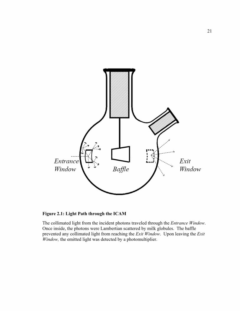
Figure 2.1: Light Path through the ICAM

The collimated light from the incident photons traveled through the Entrance Window. Once inside, the photons were Lambertian scattered by milk globules. The baffle prevented any collimated light from reaching the Exit Window. Upon leaving the Exit Window, the emitted light was detected by a photomultiplier.

22

Figure 2.2: Instrumentation to Measure Oxygen-Binding Thermodynamics of Hemoglobin

The oxygen concentration in the ICAM solution was monitored with an oxygen electrode. Spectral data was obtained using a Cary 300 spectrophotometer. The temperature of the solution was monitored with a thermistor. The device was wrapped in Tygon-tubing and temperature-controlled by flowing water from a water bath set from 4 to 50°C through the tubing.

ICAM

02 Electrode Thermistor

Spectrophotometer

23

ICAM: Stirring

The ICAM solution was stirred to keep the milk particles suspended and turbidity

at a maximum. Also, the Clark electrode requires a stirred solution for accurate

measurements.59 Below the ICAM round-bottom flask was a pneumatic stir plate housed

in a machined aluminum block. The pneumatic stir plate generated little heat during

operation, which allowed for easier temperature control of the ICAM. An air pressure of

18 psi was obtained with 2.7 revolutions per second. A Teflon-coated 2-centimeter egg-

shaped magnet was placed into the ICAM round-bottom flask and stirred the solution.

The absorbance of a solution of hemoglobin was held stable for 7 hours.

ICAM: Optical Alignment

The ICAM round-bottom flask, the oxygen electrode and thermistor, the

pneumatic stir plate housed in an aluminum block, and the camera mount were placed

inside the Cary 300 (Varian Instruments, Agilent) and covered with a Styrofoam block.

Thick felt was layered onto the Styrofoam block to ensure no outside light entered the

sample chamber. The Cary 300 was a double-beam spectrophotometer that used a series

of mirrors and baffles to switch between the reference beam and the incident beam every

33 milliseconds. The Varian Optical Spectroscopy Instrument program on Windows XP

controlled the Cary 300 and was used for measurements. Spectral data were transferred

to Excel, Graphpad 6, and Origin for analysis.

To align the optics, white light was passed through the reference and incident

windows of the Cary 300 spectrophotometer. Then, the ICAM round-bottom flask was

24

filled with 200 milliliters of a clear non-scattering solution. Alignment was achieved

when the absorbance of the emitted light was at a minimum. Next, the rubber stopper

holding the deflector was placed into the top of the ICAM round-bottom flask and the

deflector was adjusted until the absorbance was at a maximum. Afterwards, a neutral

density filter was placed in the reference beam, such that the readings from reference

beam and the incident beam were in the logarithmic range of ± 1. The ICAM

spectrophotometer was blanked for zero absorbance after adding 1% (w/v) of 1% fat milk

to the ICAM round-bottom flask. The absorbance at each of the three alignments was

consistently reproducible.

Deoxygenation of ICAM Solution Through Low Pressure Nitrogen Airflow

The ICAM solution was deoxygenated by nitrogen entering through an 18-gauge

needle inserted into a rubber stopper. The nitrogen to the first needle was provided by a

pneumatic tube attached to a nitrogen tank set at 5-15 psi. The nitrogen flowed through a

bubbler and then into the ICAM head space (fig. 2.3). This ensured the nitrogen was

water-saturated and did not dehydrate the solution. An out-flow needle attached to

pneumatic tubing ensured the pressure in the ICAM in the head space remained at lab air

pressure.

25

Figure 2.3: Flow of Water-Saturated Nitrogen Gas into the Air Space Led to Gentle Deoxygenation of the Solution

Nitrogen flow displaced oxygen in the solution in the air-tight ICAM. Two needles through a rubber stopper allowed water-saturated nitrogen inflow and air outflow over the solution. The hemoglobin deoxygenated with the solution. As the solution deoxygenated, so did the hemoglobin in the solution. Constant stirring ensured the oxygen concentration remained uniform.

26

Figure 2.4: Instrumentation to Measure Oxygen-Binding Thermodynamics of Hemoglobin

During deoxygenation of the ICAM solution, the oxygen concentration and spectral data were collected to construct the oxygen-binding curves of hemoglobin. A is the input nitrogen line and B is the output air line. C is the baffle, D is the thermistor, E is the oxygen electrode fully submerged in the solution, and F is a stir bar. The air tightness of the ICAM was ensured with rubber stoppers, shown here as cross-hatched rectangles.

27

Collimated Spectrophotometer: HPDA 8452

Collimated absorbance measurements were obtained in a Hewlett Packard Diode

Array 8452 spectrophotometer. Absorbance measurements were acquired every 2 nm

after zeroing the instrument. The half-width full-max of wavelengths for each

photomuliplier was ± 0.1 nm, and the data was collected in multiples of 100 milliseconds.

The On-Line Instrument Systems Program was used to collect data from the HPDA. The

data was exported to Excel, Graphpad 6, and Origin for further analysis.

Data Acquisition: Metmyoglobin Collimated Spectra

The spectrum of 22 µM metmyoglobin in 100 mM phosphate buffer at pH 7.4

was obtained using a HPDA 8452 spectrophotometer. A total of ten spectra were

acquired from 180 to 820 nm. Then, the ten spectra were Savitsky-Golay smoothed and

averaged.

Data Acquisition: Metmyoglobin ICAM Spectra

The ICAM spectra of metmyoglobin concentrations at various concentrations

(1100 nM, 1900 nM, 3100 nM, and 4600 nM) were taken in the ICAM

spectrophotometer. The metmyoglobin solution was added to the ICAM containing

200.0 milliliters of 100 mM phosphate buffer at pH 7.4 and 2.000 milliliters of 1% milk.

A total of ten spectra at each concentration were recorded from 500 to 750 nm. The

spectra were Savitsky-Golay smoothed and averaged for a single spectrum.

28

Data Acquisition: Obtaining the Spectrum of Oxygenated Hemoglobin in the Red Blood

Cells using Collimated Spectrophotometry

The spectra of oxygenated hemoglobin in the red blood cells were obtained using

a thin-layer two cells thick, and this eliminated nearly all the light-scattering. The cells

were centrifuged at 1000xg and the supernatant carefully removed. This process packed

the red blood cells and the sample had very high viscosity. 50.0 microliters of packed red

blood cells were placed on a microscope slide using a modified glass pipette with a large

diameter at the tip. A cover slip was gently placed on the packed red blood cells. Mild

pressure on the cover slip resulted in the packed red blood cells forming a uniform non-

scattering layer between 20 to 30 µm in thickness. The thin-layer of red blood cells was

placed in the incident beam of the HPDA 8452 spectrophotometer and the spectra were

acquired. A total of ten spectra were recorded every second. Each spectrum was

Savitsky-Golay smoothed and averaged.

Data Acquisition: Obtaining Spectrum of Oxygenated Hemoglobin in Red Blood Cell

using ICAM Spectrophotometry

The spectra of oxyhemoglobin in the red blood cells were acquired by adding 600

µL of 10% hematocrit red blood cells in 100 mM phosphate buffer at pH 7.4 with 1%

(w/v) sodium chloride to 200.0 milliliters of the same buffer with 2.000 milliliters of 1%

milk in the ICAM. A total of ten spectra was acquired from 500 to 750 nanometers with

a Cary 300 spectrophotometer. Each spectrum was Savitsky-Golay smoothed and

averaged.

29

Data Acquisition: Spectra of Oxygenated Hemoglobin at 30 µM using ICAM

Spectrophotometry

The ICAM spectra of oxygenated hemoglobin in dilute solution were obtained by

adding 3.000 mL of 2090 µM hemoglobin in 100 mM phosphate buffer at pH 7.4 to

200.0 mL of the same buffer with 2.000 mL of 1% milk in the ICAM. A total of ten

spectra were acquired from 500 to 750 nanometers with a Cary 300 spectrophotometer.

Each spectrum was Savitsky-Golay smoothed and then all spectra were averaged together

for a single spectrum.

Data Acquisition: Spectra of Oxygenated Hemoglobin at 30 µM using Collimated

Spectrophotometry

The collimated spectra of 30 µM oxygenated hemoglobin in 100 mM phosphate

buffer at pH 7.4 were taken in the HPDA 8452 spectrophotometer. A total of ten spectra

were acquired from 180 to 820 nm. Then, ten spectra were Savitsky-Golay smoothed and

averaged.

Data Acquisition: Deoxygenation of Myoglobin

The myoglobin was deoxygenated in the ICAM while the absorbance was

acquired with the Cary 300 spectrophotometer and the oxygen concentration was

acquired using the oxygen electrode. First, 200.0 µL of 310 µM myoglobin in 100 mM

phosphate buffer at pH 7.4 was added to 200.0 mL of the same buffer with 2.000 mL of

1% milk in the ICAM. The solution was deoxygenated at 22°C over the course of 75

minutes (see Deoxygenation of ICAM Solution Through Low Pressure Nitrogen

Airflow). The ICAM absorbance at 576 nm was acquired every second. The ICAM

30

absorbances were Savitsky-Golay smoothed. Oxygen electrode readings were acquired

from the YSI 5300 control panel every 20 seconds. The oxygen concentration data points

were LOWESS-fitted to estimate the oxygen concentration at every second.

2.3 Results

Overview of ICAM Spectrophotometry Validations

The goal of the work described in this chapter was to develop and validate the

instrumentation. This involved determining the two parameters of the transfer function,

validating those parameters, and verifying the measurements of the oxygen electrode

(table 2.1).

31

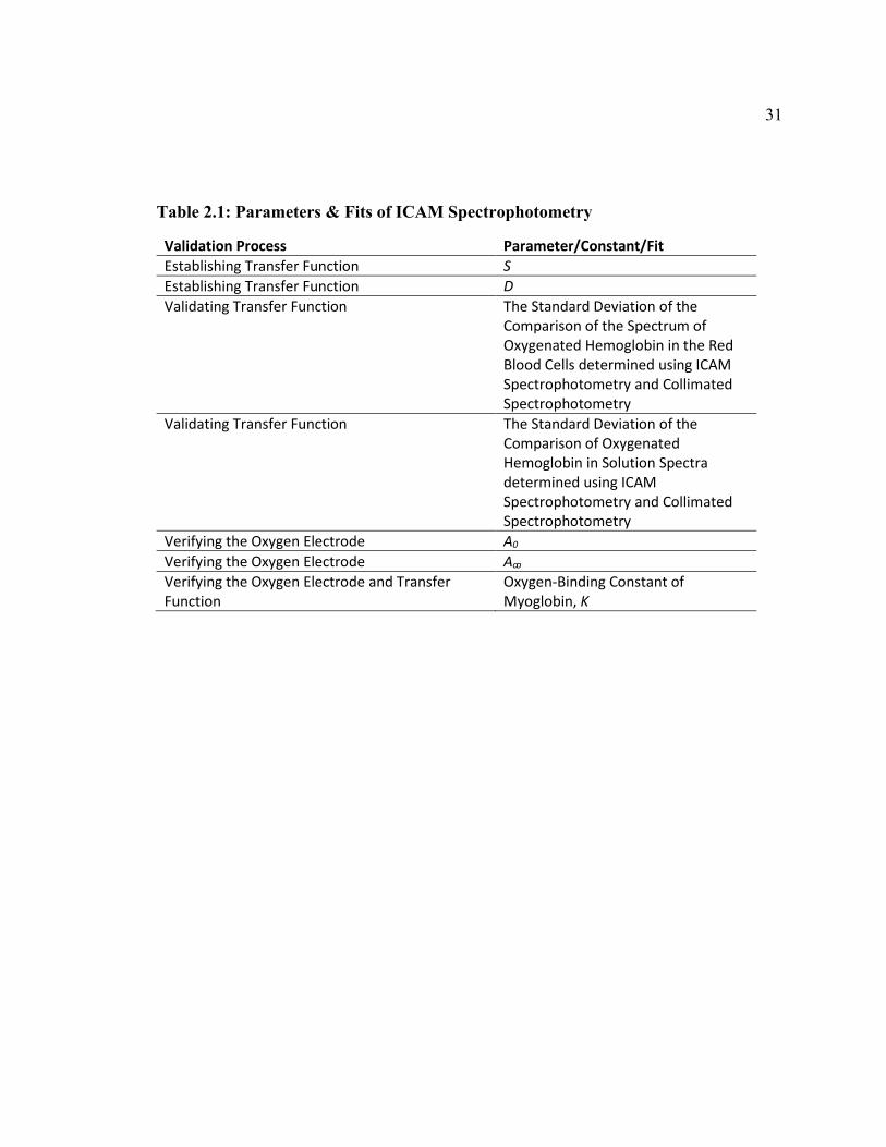
Table 2.1: Parameters & Fits of ICAM Spectrophotometry

Validation Process Parameter/Constant/Fit Establishing Transfer Function S Establishing Transfer Function D Validating Transfer Function The Standard Deviation of the

Comparison of the Spectrum of Oxygenated Hemoglobin in the Red Blood Cells determined using ICAM Spectrophotometry and Collimated Spectrophotometry

Validating Transfer Function The Standard Deviation of the Comparison of Oxygenated Hemoglobin in Solution Spectra determined using ICAM Spectrophotometry and Collimated Spectrophotometry

Verifying the Oxygen Electrode A0

Verifying the Oxygen Electrode Aꝏ

Verifying the Oxygen Electrode and Transfer Function

Oxygen-Binding Constant of Myoglobin, K

32

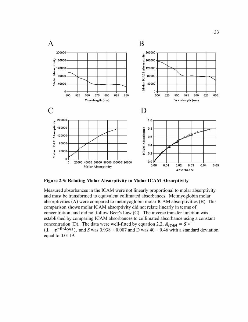
Transfer Function

The transfer function transformed ICAM absorbance (AICAM) into collimated

absorbance (ACOLL). This was necessary as the AICAM did not relate linearly with

concentration. The transfer function was:

𝐴𝐴𝐶𝐶𝐶𝐶𝐶𝐶𝐶𝐶 = −

ln(−𝐴𝐴𝐼𝐼𝐶𝐶𝐼𝐼𝐼𝐼𝑆𝑆 + 1)𝐷𝐷

. 2.1

In this equation, AICAM was the absorbance in the ICAM, S was a scalar parameter, D was

the exponential decay parameter, and ACOLL was the equivalent collimated absorbance.

Once the parameters S and D were known, it became possible to determine ACOLL from

AICAM. To determine S and D, the spectrum of metmyoglobin was acquired with and

without milk as a scattering agent. The sample with milk was placed in the ICAM, and

AICAM was acquired (figure 2.5, panel A). The sample without milk was placed in

cuvette, and ACOLL was acquired (figure 2.5, panel B). AICAM was plotted against ACOLL

and the 300 data points were fit to the inverse transfer function, equation 2.2 (figure 2.5,

panel C). Finally, S and D were determined using a Monte-Carlo fitting program in

Graphpad (figure 2.5, panel D):60

𝐴𝐴𝐼𝐼𝐶𝐶𝐼𝐼𝐼𝐼 = 𝑆𝑆 ∗ (1 − 𝑒𝑒−𝐷𝐷∗𝐼𝐼𝐶𝐶𝐶𝐶𝐶𝐶𝐶𝐶). 2.2

S was 0.938 ± 0.007, and D was 40 ± 0.46 with a standard deviation of 0.0119. The next

task was to validate the parameters S and D.

33

Figure 2.5: Relating Molar Absorptivity to Molar ICAM Absorptivity

Measured absorbances in the ICAM were not linearly proportional to molar absorptivity and must be transformed to equivalent collimated absorbances. Metmyoglobin molar absorptivities (A) were compared to metmyoglobin molar ICAM absorptivities (B). This comparison shows molar ICAM absorptivity did not relate linearly in terms of concentration, and did not follow Beer's Law (C). The inverse transfer function was established by comparing ICAM absorbances to collimated absorbance using a constant concentration (D). The data were well-fitted by equation 2.2, 𝑨𝑨𝑰𝑰𝑰𝑰𝑨𝑨𝑰𝑰 = 𝑺𝑺 ∗(𝟏𝟏 − 𝒆𝒆−𝑫𝑫∗𝑨𝑨𝑰𝑰𝑪𝑪𝑪𝑪𝑪𝑪), and S was 0.938 ± 0.007 and D was 40 ± 0.46 with a standard deviation equal to 0.0119.

34

Validation of Transfer Function using the Spectra of Oxygenated Hemoglobin in the Red

Blood Cell

The parameters S and D were validated using oxygenated hemoglobin in the red

blood cells. The spectra of oxygenated hemoglobin in the red blood cells were acquired

with and without light scattering. A thin-layer of red blood cells does not scatter light

and was used to obtain ACOLL. The sample of red blood cells with milk does scatter light

and was used to obtain AICAM. The AICAM spectrum was transformed to the ACOLL

spectrum using S and D from the metmyoglobin fitting. After normalizing at 576 nm, the

transformed ACOLL was compared to the non-scattering ACOLL. The standard deviation

between them was very low at 0.004, as shown in figure 2.6.

Validation of Transfer Function using the Spectra of Oxygenated Hemoglobin at 30 µM

The parameters S and D were validated using dilute oxygenated hemoglobin in

solution. The spectra of dilute oxygenated hemoglobin in solution were acquired with

and without light scattering. A solution of hemoglobin does not scatter light and was

used to obtain ACOLL. The solution of hemoglobin with milk does scatter light and was

used to obtain AICAM. The AICAM spectrum was transformed to the ACOLL spectrum using

S and D from the metmyoglobin fitting. The transformed ACOLL was then compared to

the non-scattering ACOLL. The two ACOLL spectra were scaled to 1 at 576 nm and

compared. This comparison fitted with a standard deviation of 0.004, indicating that the

parameters S and D are independent of the sample being measured (fig. 2.6 and 2.8).

35

500 520 540 560 580 6000.0

0.2

0.4

0.6

0.8

1.0

Wavelength (nm)

Abs

orba

nce

Absorbance Spectrum

Transformed ICAM AbsorbanceSpectrum

ICAM Absorbance Spectrum

Figure 2.6: Transformed ICAM Absorbance Overcomes Light Scattering

The absorbance spectrum of oxyhemoglobin in the red blood cells (black) agreed well with the transformed ICAM absorbance spectrum of oxyhemoglobin in the red blood cells (green, σ = 0.0045). The non-transformed ICAM absorbance spectrum of oxyhemoglobin in the red blood cells (red) did not agree well with the thin-layer absorbance spectrum of oxyhemoglobin in the red blood cells. This showed that the inverse transfer function will transform correctly measured absorbances of turbid samples to absorbance, correctly eliminating scattering artifacts. Spectra were scaled at 576 nm to correct for concentration differences.

36

Deoxygenation of Myoglobin: Validation of the Oxygen Electrode

The oxygen electrode was validated by determining the oxygen-binding constant

of myoglobin, K, and comparing it to literature values. The myoglobin oxygen-binding

equilibrium was defined as the following equation:

𝑌𝑌� =

𝐾𝐾 ∗ [𝑂𝑂2]1 + 𝐾𝐾 ∗ [𝑂𝑂2]

. 2. 3

In this equation, 𝑌𝑌 �was the fractional saturation, K was the oxygen-binding

constant of myoglobin, and [O2] was the oxygen concentration of the solution. A sample

of myoglobin was deoxygenated in the ICAM sample chamber. During the

deoxygenation process, the oxygen concentration and AICAM at 576 nm was collected.

AICAM was transformed to ACOLL using the transfer function.

The parameters A0 and Aꝏ must be acquired before the fractional saturation of

myoglobin was determined using ACOLL:

𝑌𝑌� =𝐴𝐴𝐶𝐶𝐶𝐶𝐶𝐶𝐶𝐶 − 𝐴𝐴0𝐴𝐴ꝏ − 𝐴𝐴0

. 2.4

In this equation, A0 was the absorbance of the myoglobin when none of the oxygen-

binding sites contain oxygen and Aꝏ was the absorbance with 100% of the oxygen-

binding sites contain oxygen.

Both Aꝏ and A0 were obtained through extrapolation. A0 was acquired by

substituting 𝑌𝑌� from equation 2.3 into equation 2.4, giving equation 2.5:

37

𝐴𝐴𝐶𝐶𝐶𝐶𝐶𝐶𝐶𝐶 − 𝐴𝐴0𝐴𝐴ꝏ − 𝐴𝐴0

=𝐾𝐾 ∗ [𝑂𝑂2]

1 + 𝐾𝐾 ∗ [𝑂𝑂2].

2.5

Equation 2.5 was rewritten as equation 2.6:

𝐴𝐴𝐶𝐶𝐶𝐶𝐶𝐶𝐶𝐶 =

𝐾𝐾 ∗ [𝑂𝑂2]1 + 𝐾𝐾 ∗ [𝑂𝑂2]

∗ (𝐴𝐴ꝏ − 𝐴𝐴0) + 𝐴𝐴0. 2.6

As the oxygen concentration approached 0 µM, the left-side of equation 2.6 was

eliminated, and equation 2.6 was simplified to equation 2.7 at low oxygen concentration:

𝐴𝐴𝐶𝐶𝐶𝐶𝐶𝐶𝐶𝐶 = 𝐴𝐴0. 2.7

Therefore, A0 was determined by fitting the lowest 10% absorbances and concentrations

with a linear line using Graphpad, and A0 was the y-intercept. Data from 2.5 to 3.0 µM

was plotted and A0 was 0.00086 ± 0.0002 with 6 data points in the fitting. A0 was also

confirmed by adding 20 milligrams of sodium dithionite to the deoxygenated solution of

myoglobin and the absorbance measured.

Deoxygenation of Myoglobin: Determination of Aꝏ

Aꝏ was determined through extrapolation of a double-reciprocal plot of equation

2.5. The inverse of equation 2.5 gave equation 2.8:

𝐴𝐴ꝏ − 𝐴𝐴0𝐴𝐴𝐶𝐶𝐶𝐶𝐶𝐶𝐶𝐶 − 𝐴𝐴0

=1 + 𝐾𝐾 ∗ [𝑂𝑂2]𝐾𝐾 ∗ [𝑂𝑂2] .

2.8

Equation 2.8 could be rewritten as equation 2.9:

1𝐴𝐴𝐶𝐶𝐶𝐶𝐶𝐶𝐶𝐶 − 𝐴𝐴0

= �1𝐾𝐾∗

1[𝑂𝑂2] + 1� ∗

1𝐴𝐴ꝏ − 𝐴𝐴0

. 2.9

As the oxygen concentration approaches infinity, then the left side of the equation

approaches 1, and equation 2.9 simplified to equation 2.10:

38


=1

𝐴𝐴ꝏ − 𝐴𝐴0. 2.10

Aꝏ was determined by plotting the top 10% of ACOLL with the corresponding oxygen

concentrations as 1𝐼𝐼𝐶𝐶𝐶𝐶𝐶𝐶𝐶𝐶−𝐼𝐼0

vs. 1[𝐶𝐶2]. Graphpad fitted the double reciprocal of the ACOLL

and oxygen concentrations using 18 data points from 180 to 250 µM oxygen. The y-

intercept was equal to 1𝐼𝐼ꝏ−𝐼𝐼0

, and A0 was found previously. 1𝐼𝐼ꝏ−𝐼𝐼0

was found to be 246 ±

6, and Aꝏ was 0.0049.

Deoxygenation of Myoglobin: Determination of the Myoglobin Oxygen-Binding Constant

With parameters A0 and Aꝏ elucidated, the fractional saturation, 𝑌𝑌�, could be

determined through ACOLL from equation 2.4:

𝑌𝑌� =𝐴𝐴𝐶𝐶𝐶𝐶𝐶𝐶𝐶𝐶 − 𝐴𝐴0𝐴𝐴ꝏ − 𝐴𝐴0

. 2.11

ACOLL was correlated to the oxygen concentration of the solution. As A0 and Aꝏ were

constants during the deoxygenation of myoglobin during the experiment, 𝑌𝑌� were

correlated to given oxygen concentration. 𝑌𝑌� was plotted against the oxygen

concentration and this allowed the determination of the myoglobin oxygen-binding

constant, K, by fitting the data with equation 2.3 using Graphpad:

𝑌𝑌� =

𝐾𝐾 ∗ [𝑂𝑂2]1 + 𝐾𝐾 ∗ [𝑂𝑂2]

. 2. 12

The myoglobin oxygen-binding constant was experimentally determined as 0.4800 ±

0.0022 µM-1 with 264 data points agrees well with literature values (0.54 µM-1) under

similar conditions (fig. 2.7).61,62

39

Spectral Differences of Oxygenated Hemoglobin at 30 µM and Oxygenated Hemoglobin

in the Red Blood Cell

The differences between the spectra of oxygenated hemoglobin at 30 µM and

oxygenated hemoglobin in the red blood cell were plotted on figure 2.8. The ACOLL

spectra of oxygenated hemoglobin at 30 µM and the AICAM in the red blood cell was both

obtained using the ICAM. The AICAM spectrum was transformed to the ACOLL spectrum

using S and D from the metmyoglobin fitting. The two ACOLL spectra were normalized at

576 nm. The standard deviation between the two was 0.007, with the lowest correlation

in the 510 and 560 nm region.

40

Figure 2.7: Myoglobin Oxygen-Binding Thermodynamics

𝑌𝑌� = 𝐾𝐾 ∗ [𝑂𝑂2]

1 + 𝐾𝐾 ∗ [𝑂𝑂2].

Myoglobin oxygen-binding thermodynamics were measured to validate the oxygen electrode. The transformed ICAM absorbance was compared directly to oxygen concentration using time as a constant (A). The transformed ICAM absorbance was scaled to fractional saturation by obtaining A0 and Aꝏ from the y-intercepts of panels B and C, respectively. From known A0 and Aꝏ, the fractional saturation for any given oxygen concentration can be determined from equation 2.4 (D). The equilibrium binding constant K was determined from fitting equation 2.3 to the data in panel D.

41

2.4 Discussion

Overview of ICAM Spectrophotometry Validations

The results in this chapter demonstrate that it was possible to study the oxygen-

binding thermodynamics of hemoglobin in the red blood cell. The ICAM

spectrophotometer raised the signal-to-noise significantly to overcome the very low

signal-to-noise of the scattered light that accompanies the use of red blood cells. Solving

the transfer function allowed for the transformation of the ICAM absorbances (AICAM)

into collimated absorbances (ACOLL) which were linearly related to concentration.

Finally, the oxygen electrode was tested by deoxygenating myoglobin. The validation of

the transfer function and the oxygen electrode meant the ICAM could be utilized to

compare the oxygen-binding thermodynamics of the hemoglobin in the red blood cells

and in dilute solution.

ICAM Light-Scattering

The ICAM overcame the light scattering effects of the red blood cells by

overwhelming the scattering. The ICAM instrument design had two different scatterers.

One was the deflector and the other was 1% milk in solution. Both were necessary for

the complete light scattering. Without milk, the experimental design had Mie scattering

effects, which proved challenging to overcome. A general-purpose light scattering agent

was necessary to remove the Mie scattering effects of the red blood cells. In essence,

most incident photons entering the ICAM were immediately scattered by the particles,

and the rest were scattered by the deflector. The idealized light-scattering agent would be

roughly the same size as the red blood cell with a similar refractive index to overwhelm

the effect of light-scattered of the red blood cells. Several different agents were tested,

42

such as psyllium husk powder, polyvinyl pyrrolidone with an average molecular mass of

40,000, powdered Milk (Hoosier Hill Farm, 2lbs), and milk. Milk was chosen as the milk

fat globules did not require time to dissolve in solution, did not aggregate in solution, and

was simple to reproduce the exact amount added. To maintain sterility, the milk was

used on the day it was opened.

Selection of a Standard Sample for Determining the Transfer Function Parameters

A standard sample was needed to establish whether the transfer function was

capable of transforming AICAM into ACOLL. Horse heart metmyoglobin was chosen for

three major reasons. First, metmyoglobin absorbs across the visible spectrum, and has 4

different absorption peaks at 500 nm, 542 nm myoglobin, 575m, and 632 nm to ensure

precision on the wavelength basis.63 The parameters of the transfer function were solved

using wavelengths from 500 to 650 nm, which ensured the transfer function parameters

were wavelength-independent. The second reason metmyoglobin was chosen was that it

its spectrum is pH-independent. This ensured that slight pH shifts would not significantly

perturb AICAM measurements. The third reason was that a solution of metmyoglobin does

not scatter light.

The Transfer Function Parameters S and D

Parameters S and D were determined by obtaining the spectrum of metmyoglobin

with and without milk as a scattering agent (AICAM and ACOLL, respectively). The results

showed that the ICAM spectrophotometer was more sensitive than the collimated

spectrophotometer. The ICAM spectrophotometer has a much longer pathlength because

the light scatters within the sample chamber. For instance, the ICAM round-bottom flask

43

has a diameter of 8 centimeters, but the equivalent pathlength of approximately 32

centimeters. The increased sensitivity of the ICAM is one of its useful features.

Transfer Function Validation

The parameters of the transfer function were validated using a sample that

scattered light and a sample that did not scatter light. For the first validation, red blood

cells were used as the light scattering sample. The light scattering of a suspension of red

blood cells comes from the interaction of the cell membrane with the intercellular buffer,

which has a different index of refraction. As the amplitude of visible light is smaller than

the cells, light scatters as it interacts with the cell membrane, and a solution of red blood

cells is opaque. Parkhurst showed that packed red blood cells did not scatter light, as

little buffer remained on the outside of the cells.64 The difference in the index of

refraction is removed in a packed thin-layer of red blood cells, and this method

determined the ACOLL of oxygenated hemoglobin in the red blood cells by collimated

spectrophotometry. The ACOLL spectrum was also determined using the ICAM and the

transfer function. Both ACOLL spectra were compared and agreed well. For the second

validation, the non-scattering solution used was hemoglobin in solution. The ACOLL

spectra determined from the ICAM and from collimated spectrophotometry were

compared and agreed well (fig. 2.6). This showed the parameters of the transfer function

were well determined for both scattering and non-scattering solutions. Interestingly, the

spectra of oxygenated hemoglobin in solution differed from the spectra of oxygenated

hemoglobin in the red blood cell (fig. 2.8). Spectral changes indicated a chemical

difference!

44

Deoxygenation of Myoglobin

The oxygen electrode and the deoxygenation of the ICAM were tested by

deoxygenating reduced horse heart myoglobin while monitoring both the absorbance

changes and the oxygen concentration in solution. Myoglobin was chosen for three

reasons. First, the fractional determination can be determined from absorbance

measurements. Second, it is a monomer which required fitting only one thermodynamic

parameter. Third, there were no dimerization complications to consider. The myoglobin

oxygen-binding constant determined from the ICAM spectrophotometry was 0.4800 ±

0.0022 µM-1, and the literature value was 0.54 µM-1.65 This validated the oxygen

electrode. With the transfer function and oxygen electrode verified, we determined the

oxygen binding thermodynamics of hemoglobin in the red blood cell and in solution.

45

5 0 0 5 2 0 5 4 0 5 6 0 5 8 0 6 0 00 .0 0

0 .2 5

0 .5 0

0 .7 5

1 .0 0

W a v e le n g th (n m )

AC

OL

LH e m o g lo b in in th e R B C

H e m o g lo b in in S o lu tio n

Figure 2.8: The Spectrum of Oxygenated Hemoglobin at Two Different Concentrations

The spectra of oxygenated hemoglobin in the red blood cell and in solution fit with a standard deviation of 0.007 and did not agree well. The spectral differences in the 510 nm region and the 560 nm region indicated chemical differences.

46

3. Oxygen-Binding of Hemoglobin in Solution Compared to Hemoglobin within

the Red Blood Cells at 18°C

3.1 Introduction

Contrasting Thermodynamic Models to Physiological Observations

The study of hemoglobin oxygen-binding thermodynamics depends on fitting the

oxygen-binding curve to a thermodynamic model based on physiological observations.

These fits elucidated further chemical information from the parameters determined from

the models. The thermodynamic models of hemoglobin oxygen-binding fall into two

categories: the sequential models and the concerted models. Sequential models, such as

the Adair and KNF models, assume that each oxygen binding event has a different

affinity. Cooperative oxygen binding occurs because the affinity increases as more

oxygen sites become filled. In contrast, the concerted MWC model assumes that there are

two hemoglobin conformational states and that each of those states has a fixed oxygen-

binding affinity. In concerted models, cooperativity occurs because the binding of

oxygen drives a conformation change from the low-oxygen-affinity state to the high-

oxygen-affinity state.

Adair Model: Sequential Mechanism

In 1924, Adair's dialysis experiments determined that hemoglobin consisted of

four subunits with four oxygen-binding sites.66,67 With the number of binding-sites

elucidated, Adair derived an equation for determining the fractional saturation. Each of

the oxygen-binding sites were considered chemically equivalent. Further gasometric

measurements by Adair and others were the first attempts to determine thermodynamic

constants for hemoglobin.66,67 K1 was the parameter for hemoglobin binding a single

47

oxygen molecule, K2 was the parameter for hemoglobin binding the second oxygen

molecule, and likewise up to K4. The oxygen-binding thermodynamics were determined

with the following equation:

𝑌𝑌� =

14∗𝐾𝐾𝐼𝐼[𝑂𝑂2] + 2𝐾𝐾1𝐾𝐾2[𝑂𝑂2]2 + 3𝐾𝐾1𝐾𝐾2𝐾𝐾3[𝑂𝑂2]3 + 4𝐾𝐾1𝐾𝐾2𝐾𝐾3𝐾𝐾4[𝑂𝑂2]4

1 + 𝐾𝐾1[𝑂𝑂2] + 𝐾𝐾1𝐾𝐾2[𝑂𝑂2]2 + 𝐾𝐾1𝐾𝐾2𝐾𝐾3[𝑂𝑂2]3 + 𝐾𝐾1𝐾𝐾2𝐾𝐾3𝐾𝐾4[𝑂𝑂2]4. 3.1

where 𝑌𝑌� is the fractional saturation, the numerator is the number of oxygen-binding sites

liganded, and the denominator is the total number of oxygen-binding sites.

This model is fundamental. However, it has proven to be exceedingly difficult to

obtain fits for all the binding constants. In particular, K3 is always very small, is

associated with negative cooperativity, and typically has a standard deviation of 25-

50%.32,61,68 In general, this shows that the saturating oxygen conditions are most difficult

to fit with the Adair model.69 Various mathematical and experimental attempts have been

made to resolve the error in K3, with varying levels of success.

KNF Model: Sequential Mechanism

Developed by Koshland, Nemethy, and Filmer in 1966, the KNF model supposes

that the transition from the deoxygenated and oxygenated conformations happens at the

tertiary level.69 This model argues that the two conformations observed through x-ray

crystallography do not allow for conformational changes of the monomers. In this

model, the protein conformation changes with each binding of ligand, thus sequentially

changing its affinity for oxygen at the other binding-sites. The monomers undergo

independent conformational changes, but the change of one monomer affects the others.

The number of hypothetical hemoglobin conformations ranges from five to sixteen. We

did not use the KNF model for three key reasons. First, the model does not fit

48

hemoglobin well from 𝑌𝑌� ranges below 0.025 and above 0.975, where considerable

thermodynamic information can be elucidated.70 Second, there is limited structural

evidence of more than two conformational states of the tetramer. Third, there is limited

thermodynamic evidence of more than two hemoglobin conformations in physiological

conditions. We used a thermodynamic model based on physiological observations, the

MWC model.

MWC Model: Concerted Mechanism

In 1965, Monod, Wyman & Changeux proposed an allosteric model that

comprehensively interpreted both the homotropic and hetereotropic effects of regulatory

enzymes in terms of certain features of protein structure.62 The model utilized five basic

assumptions:

1) Allosteric proteins are polymers in which the monomers are experimentally

equivalent.

2) Each monomer carries one binding site for each ligand bound. Each set of

binding sites has the same symmetry.

3) Ligand binding of one monomer imposes constraints on the conformation of

each of them

4) The protein is in an equilibrium between at least two alternative quaternary

structures which differ by distribution and energy of inter-subunit bonds and

consequently by ligand affinity for each of the binding sites.

5) When the protein goes from one state to another, its molecular symmetry is

conserved.

49

In the case of hemoglobin, it is assumed the four monomers are chemically

identical and there are two conformations based on structural data. The two

conformations are the oxygenated quaternary conformation, the R-state, and the

deoxygenated quaternary conformation, the T-state. T0,T1,T2,T3,T4 and R0,R1,R2,R3,R4

represent zero, one, two, three and four oxygens bound the T-state and R-state,

respectively. The T-state is in equilibrium with the R-state with equivalent oxygens

bound, and the parameter L is the equilibrium between T0 and R0. The parameters KT and

KR are the association constants for the T-state and R-state respectively. KT and KR are

constant no matter the number of oxygens bound to the T-state and R-state, respectively.

Due to this symmetry, an oxygen-binding fit can be derived from two conformations

using three different parameters, L, KT, and KR.

𝑌𝑌� =

𝐿𝐿 · 𝐾𝐾𝑇𝑇 · [𝑂𝑂2] · (1 + 𝐾𝐾𝑇𝑇 · [𝑂𝑂2])3 + 𝐾𝐾𝑅𝑅 · [𝑂𝑂2] · (1 + 𝐾𝐾𝑅𝑅 · [𝑂𝑂2])3

𝐿𝐿 · (1 + 𝐾𝐾𝑇𝑇 · [𝑂𝑂2])4 + (1 + 𝐾𝐾𝑅𝑅 · [𝑂𝑂2])4.

3.2

The MWC model has strong experimental evidence. Both the T-state and R-state

have been elucidated with x-ray crystallography and other techniques. There are a

maximum of three conformations based on kinetic, thermodynamic, and structural data.

Considering the experimental evidence and the fitting, this was the model chosen to fit

the data in our study.

Hill Equation & Cooperativity

Hemoglobin is an example of a cooperative protein because the binding of one

oxygen molecule increases the affinity for subsequent oxygen molecules. The utility of

the Hill equation lies in its simplicity, and this is why it is ubiquitous across hemoglobin

oxygen-binding experiments. It is a mathematical fit independent of the

50

thermodynamical model. A measure of the overall cooperativity is often presented by the

means of the maximal slope of the Hill plot:

𝑛𝑛𝑛𝑛 =𝑑𝑑𝑑𝑑𝑑𝑑𝑑𝑑 𝑌𝑌�

1 − 𝑌𝑌�𝑑𝑑𝑑𝑑𝑑𝑑𝑑𝑑 [𝑂𝑂2]

.

3.3

The Hill number, nH, is determined at a fractional saturation of 0.5. 𝑌𝑌� is the fractional

saturation, and [O2] is the oxygen concentration. Under physiological conditions, the Hill

number for hemoglobin in solution is 2.7-3.0.


Data Acquisition: Deoxygenation of Hemoglobin in Red Blood Cells (HBRBC) and

Hemoglobin in Dilute Solution (HBSOLN)

Two different samples were deoxygenated in the ICAM, the hemoglobin in

solution (HBSOLN) and the hemoglobin in the red blood cell (HBRBC). To study HBSOLN,

8.170 mL of 4.890 mM hemoglobin (heme basis) in deionized water were added to the

ICAM after blanking the ICAM spectrophotometer as discussed in “Chapter 2: Materials

& Methods.” During a separate run, 600 µL of 50% hematocrit red blood cells

suspended in 1% (w/v) NaCl in 100 mM phosphate buffer at pH 7.4 were added to a

blank ICAM to study HBRBC. Both solutions contained 4 milligrams of superoxide

dismutase (Sigma) and 20 milligrams of catalase (Thermo Fisher Scientific), which

removed any autooxidation of hemoglobin by superoxide. During both experiments, the

solution was deoxygenated at 18°C (see Control of ICAM Solution deoxygenation

through gentle nitrogen airflow from chapter 2). AICAM measurements were recorded

every second. At the same time, oxygen electrode readings were measured from the YSI

51

5300 control panel every 20 seconds. The AICAM was smoothed against time through a

23-window Savitsky-Golay filter and the oxygen concentration data points were

LOWESS-fitted to estimate the oxygen concentration at every second. After

deoxygenating both solutions by passing water-saturated nitrogen gas over the solution,

20 milligrams of sodium dithionite was added to ensure complete deoxygenation. During

the deoxygenation of HBSOLN, 30960 ACOLL measurements at 670 nm and 1548 oxygen

electrode measurements were collected. During the deoxygenation of HBRBC, 14058

ACOLL was measured at 620 nm and 703 oxygen electrode measurements were collected

(fig. 3.1).

52

0 1 0 0 0 0 2 0 0 0 0 3 0 0 0 0 4 0 0 0 0

0 .0 0

0 .0 2

0 .0 4

0 .0 6

0 .0 8

S e c o n d s

Ab

sorb

an

ceA b so r b a n c e

0

1 0 0

2 0 0

3 0 0

4 0 0

Ox

yg

en C

on

cen

tra

tio

n (µ

M)

O x y g e n

C o n c e n t r a t io n (µ M )

O x y g e n C o n c e n tr a t io n (µ M )

Ab

sorb

an

ce

0 1 0 0 2 0 0 3 0 0 4 0 00 .0 0

0 .0 2

0 .0 4

0 .0 6

0 .0 8

A B

Figure 3.1: Oxygen-Binding Thermodynamics of Hemoglobin Determined by The Relationship between Absorbance and Oxygen Concentration

The oxygen-binding thermodynamics of hemoglobin can be determined from absorbance and oxygen concentration changes during deoxygenation of the hemoglobin. A is the absorbance and oxygen concentration changes over the course of an experiment at constant temperature, and B is the direct relationship between absorbance and oxygen concentration as a function of time. A small change at the low oxygen concentration causes a large change in absorbance in the hemoglobin.

53

3.3 Results

Deoxygenation of Hemoglobin in Red Blood Cells & Hemoglobin in Solution: Fractional

Saturation

During the deoxygenation of hemoglobin in red blood cells (HBRBC) and

hemoglobin in solution (HBSOLN) in the ICAM spectrophotometer, the AICAM and the

corresponding oxygen measurements were obtained. The AICAM was transformed to

ACOLL using the transfer function described in chapter 2, and the oxygen measurements

were converted to oxygen concentration using methods described in chapter 2 and

appendix 5.6. The oxygen-binding curve required the fractional saturation to be acquired

from the ACOLL and oxygen concentration. The fractional saturation of hemoglobin is the

percent of hemoglobin oxygen-binding sites bound with oxygen. The fractional

saturation of hemoglobin, 𝑌𝑌� , for any given oxygen concentration at 620 nm was

determined by solving eq. 3.4:

𝑌𝑌� =𝐴𝐴0 − 𝐴𝐴𝐶𝐶𝐶𝐶𝐶𝐶𝐶𝐶𝐴𝐴0 − 𝐴𝐴ꝏ

. 3.4

Similarly to chapter 2, 𝑌𝑌�, the fractional saturation, was defined with three

different parameters: A0 was the absorbance of the myoglobin when none of the oxygen-

binding sites contain oxygen, Aꝏ was the absorbance with 100% of the oxygen-binding

sites contain oxygen, and ACOLL was the absorbance measurement at any given oxygen

concentration. A0 was greater than Aꝏ for any wavelength greater than 585.9 nm, and

thus equation 3.4 was different than equation 2.4. Both parameters A0 and Aꝏ must be

ascertained before the fractional saturation of hemoglobin can be determined.

54

Deoxygenation of HBRBC & HBSOLN: Determination of A0:

Both Aꝏ and A0 were found through extrapolation. The Adair equation was used

to determine Aꝏ and A0 because the MWC model does not lend itself as well to this task.

To begin, 𝑌𝑌� in the Adair relationship (equation 3.4) and in the fractional saturation

relationship (equation 3.1) were combined with to obtain equation 3.5:

𝐴𝐴0 − 𝐴𝐴𝐶𝐶𝐶𝐶𝐶𝐶𝐶𝐶𝐴𝐴0 − 𝐴𝐴ꝏ

=14∗𝐾𝐾𝐼𝐼[𝑂𝑂2] + 2𝐾𝐾1𝐾𝐾2[𝑂𝑂2]2 + 3𝐾𝐾1𝐾𝐾2𝐾𝐾3[𝑂𝑂2]3 + 4𝐾𝐾1𝐾𝐾2𝐾𝐾3𝐾𝐾4[𝑂𝑂2]4

1 + 𝐾𝐾1[𝑂𝑂2] + 𝐾𝐾1𝐾𝐾2[𝑂𝑂2]2 + 𝐾𝐾1𝐾𝐾2𝐾𝐾3[𝑂𝑂2]3 + 𝐾𝐾1𝐾𝐾2𝐾𝐾3𝐾𝐾4[𝑂𝑂2]4. 3.5

Equation 3.5 can be rewritten as equation 3.6:

𝐴𝐴0 =

14∗

𝐾𝐾𝐼𝐼[𝑂𝑂2] + 2𝐾𝐾1𝐾𝐾2[𝑂𝑂2]2 + ⋯1 + 𝐾𝐾1[𝑂𝑂2] + 𝐾𝐾1𝐾𝐾2[𝑂𝑂2]2 + ⋯

· (𝐴𝐴0 − 𝐴𝐴ꝏ) + 𝐴𝐴𝐶𝐶𝐶𝐶𝐶𝐶𝐶𝐶 . 3.6

Thus, as the oxygen concentration approaches 0 µM, the cubic and quartic

portions of the binding polynomial are greatly diminished, and equation 3.6 reduces to

equation 3.7:

𝐴𝐴0 = 𝐴𝐴𝐶𝐶𝐶𝐶𝐶𝐶𝐶𝐶. 3.7

Therefore, A0 can be determined by fitting 5186 ACOLL measurements with a quadratic

polynomial to find the y-intercept. In the case of HBSOLN, A0 was determined to be

0.0719 ± 0.00004. Similarly, A0 for deoxygenation of HBRBC was determined to be

0.00875 ± 0.00001 (fig. 3.2) using 4779 ACOLL measurements. These results were

confirmed by adding 20.0 mg of sodium dithionite to ensure complete deoxygenation.

Deoxygenation of HBRBC & HBSOLN: Determination of Aꝏ

Aꝏ was also determined through extrapolation. In this case, a reciprocal plot of

equation 3.6 gave equation 3.8:

55

𝐴𝐴0 − 𝐴𝐴ꝏ𝐴𝐴0 − 𝐴𝐴𝐶𝐶𝐶𝐶𝐶𝐶𝐶𝐶

= 4 ∗1 + 𝐾𝐾1[𝑂𝑂2] + 𝐾𝐾1𝐾𝐾2[𝑂𝑂2]2 + 𝐾𝐾1𝐾𝐾2𝐾𝐾3[𝑂𝑂2]3 + 𝐾𝐾1𝐾𝐾2𝐾𝐾3𝐾𝐾4[𝑂𝑂2]4

𝐾𝐾𝐼𝐼[𝑂𝑂2] + 2𝐾𝐾1𝐾𝐾2[𝑂𝑂2]2 + 3𝐾𝐾1𝐾𝐾2𝐾𝐾3[𝑂𝑂2]3 + 4𝐾𝐾1𝐾𝐾2𝐾𝐾3𝐾𝐾4[𝑂𝑂2]4 . 3.8

Equation 3.8 could be rewritten as equation 3.9:

1𝐴𝐴0 − 𝐴𝐴𝐶𝐶𝐶𝐶𝐶𝐶𝐶𝐶

= �4 ∗1 +𝐾𝐾1[𝑂𝑂2] + 𝐾𝐾1𝐾𝐾2[𝑂𝑂2]2 +𝐾𝐾1𝐾𝐾2𝐾𝐾3[𝑂𝑂2]3 +𝐾𝐾1𝐾𝐾2𝐾𝐾3𝐾𝐾4[𝑂𝑂2]4

𝐾𝐾𝐼𝐼[𝑂𝑂2] + 2𝐾𝐾1𝐾𝐾2[𝑂𝑂2]2 + 3𝐾𝐾1𝐾𝐾2𝐾𝐾3[𝑂𝑂2]3 + 4𝐾𝐾1𝐾𝐾2𝐾𝐾3𝐾𝐾4[𝑂𝑂2]4� ∗1

𝐴𝐴0 − 𝐴𝐴ꝏ. 3.9

As the oxygen concentration approached infinity, the equation further simplified

because the linear, square, and cubic terms become insignificant:


= �4 + ⋯+ 4𝐾𝐾1𝐾𝐾2𝐾𝐾3𝐾𝐾4[𝑂𝑂2]4

4𝐾𝐾1𝐾𝐾2𝐾𝐾3𝐾𝐾4[𝑂𝑂2]4 � ∗1

𝐴𝐴0 − 𝐴𝐴ꝏ.

3.10

Extrapolation to infinite concentration caused the left-hand side of the equation to

approach 1, and gave equation 3.11:

1𝐴𝐴0 − 𝐴𝐴𝐶𝐶𝐶𝐶𝐶𝐶𝐶𝐶

=1

𝐴𝐴0 − 𝐴𝐴ꝏ. 3.11

Therefore, Aꝏ was determined by plotting the highest 10% of absorbances as

1𝐼𝐼0−𝐼𝐼𝐶𝐶𝐶𝐶𝐶𝐶𝐶𝐶

vs. 1[𝐶𝐶2]. The y-intercept was equal to 1

𝐼𝐼ꝏ−𝐼𝐼0, and A0 was found previously. The

Aꝏ of the deoxygenation of HBSOLN was determined from 3030 data points ranging from

112-213 µM, and Aꝏ was 0.00076 ± 0.000004. The Aꝏ of the deoxygenation of HBRBC

was determined from 3030 data points ranging from 70-259 µM, and Aꝏ was 0.00135 ±

0.000006 (fig. 3.2).

56

Oxygen Concentration (µM)

Abs

orba

nce

0 3 6 9 120.055

0.060

0.065

0.070

0.075

1/[O2] (μM-1)

1/A

bsor

banc

e

0.0000 0.0025 0.0050 0.0075 0.0100100

110

120

130

140

A B

Figure 3.2: Determining the Fractional Saturation from Absorbance and Oxygen Concentration

The fractional saturation of hemoglobin was the percent oxygen bound and was linearly related to absorbance. The scaling of fractional saturation is 0 to 1, where 0 is 0% oxygen bound to hemoglobin at absorbance A0, and 1 is 100% oxygen bound to hemoglobin at absorbance Aꝏ. A0 is the y-intercept of a quadratic equation fitting at the lowest 10% of absorbance, in this case 0-10 O2 µM (A). Aꝏ is the inverse y-intercept of a linear fit of a double-reciprocal plot of the top 5% of absorbance (B). The fractional saturation of hemoglobin (𝑌𝑌�) can be determined using 𝑌𝑌� = 𝐼𝐼0−𝐼𝐼𝑋𝑋

𝐼𝐼0−𝐼𝐼ꝏ.

57

MWC & Hill Slope Fitting

The oxygen-binding curves were plotted by comparing the fractional saturation 𝑌𝑌�

to the oxygen concentration for both solutions, HBSOLN and HBRBC. The MWC

parameters of the oxygen-binding curves were determined using OriginPro 2020b. KR,

KT and L were found by Levenberg-Marquardt iterations of equation 3.2 to the oxygen

binding curves. The results of the fittings are listed on table 3.1.

The Hill coefficient nH, a common measure of cooperativity, was found by

plotting log [𝐶𝐶2]1−[𝐶𝐶2]

against log 𝑌𝑌�and finding the maximal slope, which is when 𝑌𝑌� is 0.5.

Table 3.1: Hemoglobin Oxygen-Binding Parameters in Solution and in the RBC (18°C)

Parameter Hemoglobin in RBC Hemoglobin in Solution Difference (%) nH 2.475 ± 0.2% 2.949 ± 0.1% 16

𝑋𝑋� (µM) 15.17 ± 0.1% 18.83 ± 0.1% 30 L 870 ± 1.0 % 9830 ± 1.4% 91

KR (µM-1) 0.353 ± 0.3% 0.532 ± 0.4% 33 KT (µM-1) 0.0080 ± 0.4% 0.0061 ± 0.3% -24

58

Comparison of the Hemoglobin Oxygen-Binding Parameters in Solution and in the RBC

at 18°C

All of the hemoglobin oxygen-binding parameters of hemoglobin were different

in RBC (HBRBC) versus in solution (HBSOLN). First, the Hill number was 16% smaller in

RBCs, indicating that HBRBC releases oxygen to the tissues over a wider concentration

than would be predicted from HBSOLN measurements. 𝑋𝑋� is the oxygen activity at half-

saturation, a measure of oxygen affinity. In the red blood cells, 𝑋𝑋� is 30% lower than in

solution. This indicated that oxygen is released at lower concentrations that would be

predicted from solution measurements.

The differences between HBSOLN to HBRBC were even larger for the three

parameters of the MWC model. The largest difference was in the parameter L that

differed by 91%. Since L is the ratio of oxygen-free T-state hemoglobin divided by

oxygen-free R-state hemoglobin, the difference indicates that HBRBC favors the T-state.

The KR value for HBRBC is smaller by 33% than in solution indicating stronger oxygen

affinity of the R-state. In contrast, KT is the only value that increases in RBCs compared

to solution. The oxygen affinity of the expanded deoxygenated T-states was 24% higher

in RBCs, indicating that HBRBC bound oxygen considerably weaker than in solution.

The differences between the HBRBC and HBSOLN oxygen binding curves are

correlated with spectral differences of oxygenated hemoglobin in the RBC and in

solution. The major differences are in the oxygenated spectra. The 576/560 nm ratios for

oxyhemoglobin in the erythrocyte and in solution are 1.42 and 1.63, respectively. These

59

differences between cellular hemoglobin and solution hemoglobin reflect the

environmental dependence of the relaxed conformations.

3.4 Discussion

We have validated the components of our system in several ways. One of the

most relevant is that our binding parameters for hemoglobin in solution are in very good

agreement with literature values. Published values for the three MWC parameters, L, KR,

and KT were 9100, 0.532 µM-1, and 0.0069 µM-1, respectively.62 We report values of

9480, 0.532 µM-1, and 0.0061 µM-1, respectively (table 3.1). When curves are generated

using these two sets of values, the standard deviation of the fit is very small at 0.0028

(fig. 3.3).

Our binding parameters for hemoglobin in red blood cells shows that

encapsulation within the RBC results in significantly lowered co-operativity and higher

oxygen affinity than in solution (fig. 3.4). First, the lowered cooperativity of HBRBC

compared to HBSOLN is established by our nH values of 2.475 and 2.976, respectively.

Literature values are in the same range as ours but not nearly as precise. Multiple

gasometric studies of hemoglobin-oxygen binding in the RBC have reported Hill

numbers ranging from 2.5 to 3.3.32,67,71–73 Recently, transient absorption microscopy was

used to study oxygen binding in a single red blood cell.74 Only six data points were

obtained for the oxygen binding curve and the reported nH of 3.5 differs markedly from

this study.

60


Fra

ctio

na

l S

atu

rati

on

(Y

)

0 1 0 2 0 3 0 4 0 5 00 .0 0

0 .2 5

0 .5 0

0 .7 5

1 .0 0

H e m o g lo b in L ite ra tu re V a lu e

H e m o g lo b in in S o lu t io n F i t

Figure 3.3: Hemoglobin Oxygen-Binding Compared to Literature

The fits of the hemoglobin in solution discussed in this chapter were plotted against literature values. The fits were in good agreement (σ = 0.0028)

61


Ox

yg

en C

on

cen

tra

tio

n (µ

M)

0 2 0 4 0 6 0 8 0 1 0 00 .0 0

0 .2 5

0 .5 0

0 .7 5

1 .0 0H e m o g lo b in in th e R B C

H e m o g lo b in in S o lu tio n

Figure 3.4: Difference of Hemoglobin Oxygen-Binding in Different Environments

Hemoglobin in the red blood cell showed greater affinity for oxygen than hemoglobin in solution with less co-operativity.

62

The increased affinity of HBRBC is demonstrated by our reported affinity of 15.63

µM compared to our reported affinity of 18.83 µM for HBSOLN. Our HBSOLN affinity is

similar to values reported in the literature.32,72,73 The closest equivalent for our HBRBC

measurements is a thin-layer study that yielded half-saturation values for oxygenated

HBRBC in good agreement with the values reported herein.75 However, that study did not

make a direct comparison with hemoglobin free in solution.

Deeper mechanistic insights were obtained by elucidating the MWC parameters

for HBRBC and HBSOLN. The largest difference, 92%, was for L, the ratio of the T- to R-

state populations in the absence of oxygen. L was 870 in the red blood cell and 9830

when free in solution. This dramatic decrease in the population of the lower-affinity

structure in the red blood cell explains in part its higher oxygen affinity.

The relative binding constants also support the observation of higher affinity in

the red blood cell. Specifically, the binding constant, KR, for HBRBC is approximately

24% greater than in solution. Likewise, KT for HBRBC is a 43% greater than in solution.

Taken together, these parameters indicate higher affinity of the hemoglobin molecule for

oxygen when packed in the erythrocyte. These differences are seen in the left-shifted

oxygen binding curve of HBRBC compared to that of free hemoglobin (fig. 3.4). The few

studies that have measured these MWC parameters in red blood cells have not made

direct comparison with hemoglobin free in solution. Of those, one thin-layer study

reported thermodynamic parameters at 37°C and pH 7.4 that were associated with very

large uncertainties.74 As a result, their reported KT and calculated KR values overlap

within error, and is consistent with no T-state to R-state conformational change upon

63

oxygenation. Such a finding conflicts with our basic understanding of hemoglobin. Also

in that paper, L was 16 million, a dramatically different value from that of 870 reported

herein.

The concentration of hemoglobin in red blood cells is 23-24 mM, more than half

of the concentration in the crystal. In contrast, solution measurements of hemoglobin

typically use about 100 µM to obtain precise data and to prevent dissociation into non-

cooperative dimers. We suggest that this approximately 250-fold difference between the

concentrations of hemoglobin in solution and in erythrocytes gives rise to significantly

different molecular behavior. The higher affinity of the confined hemoglobin must be

related to the close proximity of the hemoglobin in the red blood cell, as supported by the

differences in the absorbance spectra in both environments. The difference is

significantly greater for the oxy spectra, which is primarily R-state hemoglobin. We

postulate that the R-state conformation in the erythrocyte that is altered relative to both

the crystal and solution structures.

The long-held assumption that the binding and release of O2 from HBSOLN is the

same as HBRBC is disputed by results presented herein. The behavior of hemoglobin in its

natural cellular environment is significantly different. From a physiological perspective,

the variable demands of the plethora of organs and tissues in the human body are better

satisfied with a less cooperative release of oxygen from hemoglobin. We find that the

encapsulated, packed hemoglobin unloads its oxygen in a more evenly distributed process

than has been previously reported.

64

4. Comparison of Thermodynamics of Oxygen-Binding of Hemoglobin in

Solution versus Hemoglobin in the Red Blood Cell

4.1 Introduction

The cooperativity of hemoglobin has been described as a “molecular lung in reverse,”

decreasing in size as the deoxygenated T-state hemoglobin binds oxygen and undergoes a

conformation changes to the compacted R-state. The T-state hemoglobin is called the

tense-state of hemoglobin due to a series of salt bridges that lock different helices in

place, as described in chapter 1. As T-state hemoglobin binds oxygen, the salt bridges are

broken and entropy increases as the hemoglobin adopts a relaxed conformation, or the R-

state. While hemoglobin binding oxygen is exothermic and exergonic under

physiological conditions, much experimental evidence shows that the thermodynamic

driving-force for HBSOLN was the large increase of energy during the transition from T-

state to R-state.

Detailed thermodynamic information about the transition between T-state to R-state

hemoglobin can be determined from the binding isotherms of hemoglobin in solution

(HBSOLN) and hemoglobin in the red blood cell (HBRBC). The Gibbs free energy (ΔG),

the enthalpy (ΔH), and the entropy (ΔS) can be determined for each MWC parameter, KR,

KT, and L, by determining the oxygen-binding curves of HBSOLN and HBRBC of different

isotherms. By keeping the temperature constant and determining the KR, KT and L of

equation 3.2, the ΔG of each parameter for each determined temperature can be solved by

equation 4.1.

𝛥𝛥𝛥𝛥 = −𝑅𝑅𝑅𝑅 · 𝐿𝐿𝑛𝑛 𝐾𝐾𝑒𝑒𝑒𝑒 . 4.1

65

In this equation, R is the gas constant 1.987 cal·K-1·mol-1, T is the temperature in

Kelvin, and Keq is the thermodynamic parameter. The Gibbs free energy equation 4.2

relates the enthalpy and entropy to the Gibbs free energy.

𝛥𝛥𝛥𝛥 = 𝛥𝛥𝑛𝑛 − 𝑅𝑅 · 𝛥𝛥𝑆𝑆. 4.2

By combining equations 4.1 and 4.2 using 𝛥𝛥𝛥𝛥 and rewriting, equation 4.3 can be

determined:

𝐿𝐿𝑛𝑛 𝐾𝐾𝑒𝑒𝑒𝑒 = −𝛥𝛥𝑛𝑛𝑅𝑅 · 𝑅𝑅

+ 𝛥𝛥𝑆𝑆. 4.3

Assuming that the heat capacity and entropy of the parameter remain constant, the

equation can be modified to fit the equilibrium constants of the same reaction at two

different temperatures, shown in equation 4.4:

𝐿𝐿𝑛𝑛 𝐾𝐾1𝐾𝐾2

= −𝛥𝛥𝑛𝑛𝑅𝑅�

1𝑅𝑅2−

1𝑅𝑅1� + 𝛥𝛥𝑆𝑆. 4.4

In equation 4.4, K1 as the equilibrium constant for the reaction at temperature T1, and K2

is the equilibrium constant for the reaction at temperature T2. From this derivation,

equation 4.4 can be applied to multiple temperatures with multiple equilibrium constants

by using equation 4.5:

𝛥𝛥𝑛𝑛 = −𝑅𝑅 ·

𝑑𝑑 𝐿𝐿𝑛𝑛 𝐾𝐾𝑒𝑒𝑒𝑒

𝑑𝑑 1𝑅𝑅

. 4.5

This equation states that the enthalpy is the slope of a linear fit of the Ln Keq plotted

against inverse temperature (in Kelvin). The enthalpy and Gibbs free energy for KR, KT,

L and 𝑋𝑋� can be determined from equations 4.1 and 4.4, and utilizing those values, the

entropy can be determined from equation 4.2. From the ΔH, ΔS, and ΔG of the

66

thermodynamic parameters of KR, KT, L and 𝑋𝑋� of HBRBC and HBSOLN, insights into the

energy that drives the hemoglobin oxygen-binding reaction can be elucidated.


Data Acquisition: Deoxygenation of Hemoglobin in the Red Blood Cell and Hemoglobin

in Solution at Varying Temperatures

AICAM and oxygen concentrations were obtained during the deoxygenation of

HBRBC and HBSOLN at varying temperatures. The protocols, concentrations, and

measurements were described in chapter 3. Hemoglobin in the red blood cells were

deoxygenated at 18, 20, 26, 32, and 37 °C, and hemoglobin in solution was deoxygenated

at 14, 18, 20, and 25 °C. The temperature was maintained using temperature-controlled

water flowing through Tygon tubing. The temperature was maintained at ± 0.1 °C during

the deoxygenation. Each deoxygenation took place over the course of 4 to 8 hours.

AICAM was collected every second and oxygen electrode measurements were taken every

20 seconds. As previously described, AICAM was transformed to ACOLL, and the oxygen

electrode measurements for every second was extrapolated.

Deoxygenation of HBRBC & HBSOLN: Determination of A0, Aꝏ, Cooperativity, and

Thermodynamic Parameters

The determination of the asymptotes, cooperativity, and thermodynamic

parameters for the deoxygenation of HBRBC and HBSOLN are fully described in chapter 3

(fig. 3.1). A0 was found through extrapolation of the plots of ACOLL versus oxygen

concentration and Aꝏ was determined from the extrapolation of the double reciprocal of

the same plot. The MWC parameters KR, KT, and L were found in OriginPro 2020b using

Levenberg-Marquardt iterations.

67

Deoxygenation of HBRBC & HBSOLN: Determination of Enthalpy, Entropy, and Gibbs Free

Energy of KR, KT, and L

The ΔH for KR, KT, and L, were determined from a linear fit of Ln (Keq) versus T-1

plot. The slope of the fit was −𝛥𝛥𝛥𝛥𝑅𝑅

as described by equations 4.3, 4.4 and 4.5, and no

abnormal heat capacities were found (fig. 4.2-4.4). ΔG of each thermodynamic

parameter was found from equation 4.1. ΔS was found by using known parameters ΔH

and ΔG in equation 4.2. ΔG was determined from equation 4.1 after obtaining ΔG and

ΔS.

4.3 Results

To determine the thermodynamics of the hemoglobin-oxygen equilibrium, the

oxygen binding isotherms were obtained at several different temperatures (fig. 4.1 and

4.2). The HBRBC experiments were carried out at five temperatures ranging from 18 to 37

°C (fig. 4.1). These temperatures were chosen to cover a range of near physiological.

The HBSOLN experiments were carried out at only four temperatures ranging from 13 to

25 °C (fig. 4.2). The experiment could not be carried out at 37 °C because hemoglobin

tetramers dissociate to dimers precipitated over the time course of the experiment.

There were significant differences in the temperature dependence of oxygen-

binding affinity for HBRBC and HBSOLN. For instance, 𝑋𝑋�, the oxygen concentration of the

solution at the half-saturation of hemoglobin, for HBRBC increased 1.51-fold (from 15.17

to 22.86 µM oxygen) as the temperature was increased from 18 to 26 °C. In contrast, the

𝑋𝑋� for HBSOLN increased 2.45-fold (from 11.75 to 28.90 µM oxygen) over almost the same

temperature range (from 18 to 25 °C). When the isotherms were fit using a hyperbolic

68

equation that assumes a single-binding site and no cooperativity, there were much larger

fitting errors of 14.4% (appendix 5.4).

To gain mechanistic insights about the energetics of the hemoglobin-oxygen

equilibrium, the oxygen binding curves in figures 4.1 and 4.2 were fitted to the MWC

model and the resulting three parameters were analyzed using a van’t Hoff plot (figs. 4.3,

4.4, and 4.5). The slope of the plot for L (slope = -∆HL/R) was negative for both HBSOLN

and HBRBC (figure 4.3). This indicated that heat was absorbed when hemoglobin made

the transition from its low-affinity T-state to its high-affinity R-state in the absence of

bound oxygen. More important is that the magnitudes of the slopes were very different.

About three times more enthalpic heat was required in the red blood cell (∆HL = 10.4

kcal/mol) than in solution (∆HL = 3.2 kcal/mol). Significantly more energy was needed

to make the conformational transition in the red blood cell. The entropic energy

differences (y-intercepts = ∆SL/R) between the two systems were 50.8 cal/mol•K in red

blood cells and 29.5 in solution. This 1.7-fold larger entropic energy indicated

significantly more order (or, fewer microstates) was involved in the conformational

transition within the cells than in solution.

The slopes of the van’t Hoff plots for KT and KR were all positive, indicating that

energy was released by oxygen bound to either state. The nearly overlapping lines of the

KT van’t Hoff plots indicated only minor differences between the two systems (fig. 4.4).

The enthalpies for oxyhemoglobin formation in the low-affinity T-state were -4.5

kcal/mol in red blood cells and -3.6 kcal/mol in solution. The entropies showed slightly

larger differences at -25.3 cal/(mol·K) in red blood cells and -22.6 cal/(mol·K) in

solution. The differences were much greater for KR.

69

The slopes of the van’t Hoff plots for KR in the two systems gave enthalpies of -

5.2 kcal/mol in red blood cells and -11.5 kcal/mol in solution (fig. 4.5). This nearly two-

fold difference indicated that more heat energy is released when oxygen binds to R-state

hemoglobin in solution than it does in the cell. An even more profound difference was

observed for the entropies, in which a change of sign was observed. In red blood cells,

the entropy associated with KR was – 20.1 cal/(mol·K). In contrast, that parameter was –

40.6 cal/(mol·K) in solution. It seems that R-state hemoglobin loses order when it binds

oxygen in red blood cells, but gains order in solution. The thermodynamic differences

between the ratios of 𝐾𝐾𝑇𝑇𝐾𝐾𝑅𝑅

for HBRBC and HBSOLN was most adequately described as

changes in KR.

70

Figure 4.1: Oxygen-Binding Curves of HBRBC at Different Temperatures

The oxygen-binding curves at 18, 20, 26, 32, and 37 °C of HBRBC are shown here from A-E, respectively. The oxygen-binding affinity decreases at the temperature increases, shown in F. The data is shown as the black dots and the blue line is the fit using eq. 3.2 (MWC binding polynomial). The error residuals are in red and relate to the right-hand Y-axis.

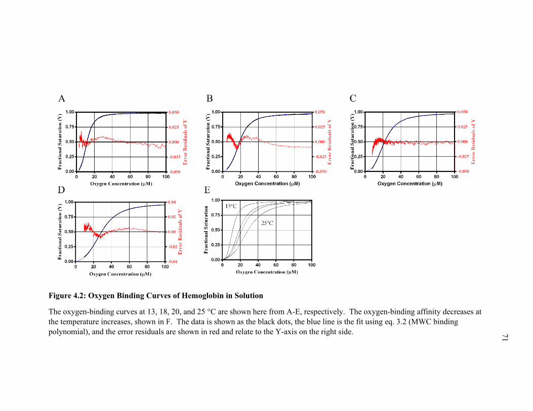
71

Figure 4.2: Oxygen Binding Curves of Hemoglobin in Solution

The oxygen-binding curves at 13, 18, 20, and 25 °C are shown here from A-E, respectively. The oxygen-binding affinity decreases at the temperature increases, shown in F. The data is shown as the black dots, the blue line is the fit using eq. 3.2 (MWC binding polynomial), and the error residuals are shown in red and relate to the Y-axis on the right side.

72

1 /K (T e m p e r a tu r e )

Ln

(L

)

0 .0 0 3 0 0 0 .0 0 3 2 5 0 .0 0 3 5 0 0 .0 0 3 7 5 0 .0 0 4 0 06

7

8

9

1 0

H B S O L N

H B R B C

Figure 4.3: Van’t Hoff Plots for L

The natural log L values obtained from the data shown in figure 4.1 for HBRBC (in black) and 4.2 for HBSOLN (in red) with the linear fits to the van’t Hoff equation.

73


Ln

(K

T)

0 .0 0 3 0 0 0 .0 0 3 2 5 0 .0 0 3 5 0 0 .0 0 3 7 5 0 .0 0 4 0 0-5 .6

-5 .3

-5 .0

-4 .7

H B S O L N

H B R B C

Figure 4.3: Van’t Hoff Plots for KT

The natural log KT values obtained from the data shown in figure 4.1 for HBRBC (in black) and 4.2 for HBSOLN (in red) with the linear fits to the van’t Hoff equation.

74


Ln

(K

R)

0 .0 0 3 0 0 0 .0 0 3 2 5 0 .0 0 3 5 0 0 .0 0 3 7 5 0 .0 0 4 0 0-1 .8

-1 .2

-0 .6

0 .0

H B S O L N

H B R B C

Figure 4.5: Van’t Hoff Plots for KR

The natural log KR values obtained from the data shown in figure 4.1 for HBRBC (in black) and 4.2 for HBSOLN (in red) with the linear fits to the van’t Hoff equation.

75

Table 4.1: Oxygen-Binding Thermodynamic Parameters

Thermodynamic Parameter

HBRBC HBSOLN Myoglobin in Solution

ΔGL (20°C) (kcal/mol) -4.1 ± 1.8% -5.4 ± 1.8% ΔGKT (20°C) (kcal/mol) -5.1 ± 0.3% -5.0 ± 0.4% ΔGKR (20°C) (kcal/mol) -7.4 ± 0.4% -7.6 ± 0.4% ΔG = -7.6 ΔHL (kcal/mol) 10.7 ± 9.6% 3.3 ± 8.7% ΔHKT (kcal/mol) -4.5 ± 4.6% -3.6 ± 26.6% ΔHKR (kcal/mol) -5.2 ± 4.0% -11.5 ± 11.3% ΔH = -13.5 ΔSL (cal/mol·K) 50.8 ± 4.6% 29.5 ± 3.3% ΔSKT (cal/mol·K) -25.3 ± 2.1% -22.6 ± 14.7% ΔSKR (cal/mol·K) -20.1 ± 3.5% -40.6 ± 11.1% ΔS = -18

The hemoglobin values were obtained from van’t Hoff plots in figures 4.3, 4,4, and 4.5. The myoglobin values were obtained from similar plots that are not shown.

76

4.4 Discussion

The results in this chapter indicate that there are significant differences in the oxygen-

binding affinity and cooperativity of HBRBC and HBSOLN. These differences are best

described by differences in the MWC parameters KR and L. The parameter KT showed

little difference between the two. Similarly, the oxygenated R-state of HBRBC and

HBSOLN had starkly different spectra, whereas the deoxygenated T-state of HBRBC and

HBSOLN had similar spectra. The different spectra and thermodynamic values for ΔHKR,

ΔGKR, and ΔSKR indicated that the R-state chemistry differed between HBRBC and

HBSOLN.

The global allostery model of hemoglobin put forward by Imai provides an

explanation how hemoglobin can have different properties in solution versus in the red

blood cell. Imai hypothesizes that there is an ensemble of minor conformational states

within the R-state that result in the different oxygen-binding thermodynamics of the R-

state. These minor conformational states depend on conditions such as proton

concentration, salt type and concentration, and the type and concentration of the allosteric

effector (2,3-diphosphoglycerate, inositol, or others). The experiments described in this

chapter add to this list by revealing that encapsulating hemoglobin in red blood cells,

HBRBC, primarily affects the R-state.

The values we obtained for the oxygen-binding parameter KR are similar to

myoglobin single-site thermodynamics in the literature. Reported values for myoglobin

oxygen-binding ΔH, ΔG, and ΔS were -13.5 kcal/mol, -7.6 kcal/mol (20°C), and -18

cal/(mol·K), respectively. Our HBSOLN R-state ΔH, ΔG, and ΔS were similar at -11.5

kcal/mol, -7.6 kcal/mol, and -40.6 cal/(mol·K). In contrast, our HBRBC R-state

77

parameters were much different with ΔH, ΔG, and ΔS for KR of -5.2 kcal/mol, -7.4

kcal/mol, and -20.1 cal/(mol·K). Most striking difference is that the entropy, which

indicates a fundamental change in the R-state when it is in red blood cells.

One of the most significant differences of oxygen-binding between HBSOLN and

HBRBC was the MWC parameter L. L is an endothermic constant which describes the T-

state population divided by the R-state population at zero oxygen concentration. At

20°C, ΔGL is more exergonic for HBSOLN than HBRBC, indicating a decrease in oxygen-

binding affinity. While the ΔSL greatly increased from HBSOLN to HBRBC, the smaller

endothermic ΔHL for HBSOLN as compared to HBRBC overcame the effects of ΔSL. We

propose the difference in L results from a difference in hemoglobin solvation, in which

water is more oriented on the hemoglobin surface in red blood cells. Numerous

experiments show that the T-state is more stable than the R-state at zero oxygen

concentration.76,77 The ratio of surface area to volume increases from the T-state to the

R-state. Furthermore, the surface area of the R-state is more hydrophobic than the T-

state. The difference between the hydrophobic surface area of the R-state to the T-state is

roughly 420 Å2 based on Kyte-Doolittle simulations. This equates to 67 ordered water

molecules, as confirmed through osmotic pressure experiments.78 The hemoglobin

hydration shell effect is likely to be the major cause of the loss of approximately 20

cal/(mol·K) entropic energy when comparing HBRBC to HBSOLN. It is significant because

red blood cells are 96% hemoglobin by dry weight and 35% (w/w) of the total content.79

As a result, each hemoglobin tetramer in the red blood cell is hydrated by about 6800

water molecules, with a significant portion of them bound in the first and second

hydration spheres and leaving little for bulk water. In fact, other researchers have already

78

found that the rate-limiting step of hemoglobin cooperativity is the ordered binding of

water molecules to the extra protein surface exposed on the transition from the low-

affinity T to the high-affinity R-state of hemoglobin.78 Due to the high concentration of

hemoglobin in the red blood cell (fig. 1.2), there are hemoglobin-hemoglobin interactions

that would not occur nearly as frequently in HBSOLN, which may block the R-state of

HBRBC from binding as many waters in the hydrophobic regions as the R-state of HBSOLN.

This difference suggested that the dehydrated environment of the red blood cell

facilitated a shift from the T-state to the R-state as compared to HBSOLN. This suggests

that water should be considered an allosteric effector of hemoglobin.

Another of the most significant differences of oxygen-binding between HBSOLN

and HBRBC was the MWC parameter KR. KR is an endothermic constant which describes

oxygen-binding of the R-state. At 20°C, ΔGKR is slightly more exergonic for HBSOLN

than HBRBC, indicating a decrease in oxygen-binding affinity. While the ΔSKR greatly

decreased from HBSOLN to HBRBC, the larger exothermic ΔHKR for HBSOLN as compared

to HBRBC overcame the effects of ΔSKR. We propose the difference in KR results from a

difference in hemoglobin solvation, in which water is more oriented on the hemoglobin

surface in red blood cells. We propose that HBRBC forms octamers or higher order

quaternary structures in the red blood cell for the R-state. Higher order quaternary

structures have been elucidated for concentrated sickle hemoglobin, and these are

hypothesized to be sickle cell fibrils displayed in the sickle red blood cells.80 Higher

order quaternary structures above tetramers have been verified in several experiments

with hemoglobin A, but these conditions are not under physiological conditions.81–84 The

increased concentration of the red blood cell may induce further hemoglobin tetramer

79

interaction than hemoglobin in dilute solution. The R-state would be more affected than

the T-state due to the increased interaction of the hydrophobic surface areas between two

tetramers, causing a difference in ΔSKR.

Further experiments would elucidate the higher order quaternary states of

hemoglobin in the red blood cell. FRET acceptor-donor experiments with increasing

hemoglobin concentration in microgels could show the octamer formation at a certain

concentration.85,86 The concentration within the red blood cell can be increased and

decreased with osmotic pressure. Aa solute that does not cross the membrane nor acts as

an allosteric effector could affect the osmotic pressure. As the osmotic pressure increases

or decreases, the hemoglobin concentration changes in the red blood cell. Elucidating the

oxygen-binding curve in these conditions could add further understanding of oxygen-

binding thermodynamics of hemoglobin in the red blood cell, and continue further

knowledge of human oxygen-binding delivery for the body.

5. Appendix

5.1 MWC Oxygen-Binding Thermodynamic Parameters

The van’t Hoff plots of the deoxygenation of HBRBC and HBSOLN were linearly

determined from the three MWC thermodynamic parameters. The three MWC

thermodynamic parameters were globally fitted using OriginPro. The thermodynamic

parameters of the oxygen-binding curves of HBRBC and HBSOLN are reported in tables 5.1

and 5.2, respectively.

80

Table 5.1: MWC Parameters of Hemoglobin in Solution

Temperature L KR KT 13°C 9120 ± 2.0% 0.833 ± 0.5% 0.0071 ± 0.7% 18°C 9830 ± 1.4% 0.532 ± 0.4% 0.0061 ± 0.3% 20°C 10330 ± 1.8% 0.466 ± 0.5% 0.0056 ± 0.4% 25°C 11480 ±1.1% 0.369 ± 0.8% 0.0055 ± 0.2%

Listed here are the MWC parameters of the oxygen-binding curves of hemoglobin in solution

Table 5.2: MWC Parameters of Hemoglobin in the Red Blood Cell

Temperature L KR KT 18°C 860 ± 2.0% 0.352 ± 0.5% 0.0071 ± 0.7% 20°C 1090 ± 1.8% 0.337 ± 0.4% 0.0061 ± 0.3% 26°C 1680 ± 1.6% 0.274 ± 0.6% 0.0058 ± 0.4% 32°C 2460 ± 2.3% 0.243 ± 0.5% 0.0056 ± 0.4% 37°C 3420 ± 2.0% 0.199 ± 0.1% 0.0055 ± 0.2%

Listed here are the MWC parameters of the oxygen-binding curves of hemoglobin in the red blood cell

81

5.2 Wavelength Dependent Effects

In earlier studies, it was found that the oxygen-binding curve of hemoglobin in

solution had wavelength-dependent effects from 515-585 nm.87,88 Any

spectrophotometric study in this region must consider that the percent oxygen bound to

hemoglobin does not relate linearly with Beer’s law. Such data must therefore be

globally fit to accurately determine binding constants for this process. The oxygen-

binding curve of hemoglobin from 615-650 nm measured in the ICAM was found to be

wavelength-independent. In a single deoxygenation experiment, the oxygen-binding

curves were determined at each individual wavelength from 615-650 nm, and the

differences in fractional saturation between the wavelengths was found to be within the

error of the ICAM spectrophotometer, and no pattern could be established. In the present

studies, measurements were obtained at 620 nm, where fractional absorbance changes

correspond directly to fractional ligand binding and require no additional global fitting.

5.3 Buffers and the Intracellular Chemical Environment of the Red Blood Cell

Hemoglobin oxygen-binding is greatly affected by allosteric effectors, as determined

by Bohr and others.89,90 In addition, the red blood cell membrane was a hurdle for our

experiments, as concern that any differences between the intracellular environment and

the external environment would skew the oxygen-binding of hemoglobin as compared to

hemoglobin in solution. As such, phosphate-buffered saline (PBS) was used. At 100

mM, phosphate maximally mimics the diphosphoglycerate (DPG) effect of blood

plasma.89 Phosphate can pass through the cell membrane equally as well as DPG. Any

DPG that might have remained in the red blood cells after multiple washes would be

overwhelmed by the phosphate, as the hemoglobin in solution would be allosterically

82

affected in the same manner. Additionally, the pH of phosphate buffer minimally

changes from 14°C-37°C. While the pH meter was calibrated at the desired temperature,

this made pH adjustments minimal. Also, the PBS buffer contained 1% (w/v) sodium

chloride. This kept the red blood cells isotonic at physiological salt concentrations.

5.4 HBRBC Oxygen-Binding Thermodynamics Assuming No Cooperativity

At low hemoglobin concentration and high oxygen content, the hemoglobin

tetramer can dimerize into αβ subunits.91 The dimer has no cooperativity, and the two

binding sites of each monomer is equivalent. The dissociation constant of hemoglobin

(KD) from tetramer/dimer at room temperature in phosphate-buffered saline is 1 µM-1.

KD increases up to 25 µM-1 at 37°C. Keeping the HBSOLN concentration above 150 µM

effectively eliminated the tetramer/dimer dissociation at room temperature. At higher

temperatures, the concentrations necessary to eliminate tetramer/dimer dissociation was

beyond the detection of the ICAM spectrophotometer. The oxygen-binding of HBRBC

assuming a single binding constant can be reduced to eq. 5.1:

𝑌𝑌� =

𝐾𝐾 ∗ [𝑂𝑂2]1 + 𝐾𝐾 ∗ [𝑂𝑂2]

. 𝟔𝟔.𝟏𝟏

The equation was written for each individual monomer of hemoglobin, but if the

binding sites are equivalent, then K can be scaled to dimers by halving it. The fits of

HBRBC deoxygenation from chp.4 did not fit well (fig. 5.2). The average standard

deviation had 14.4% error (table 5.3). This result shows that tetramer/dimer dissociation

was very low.

83

Figure 5.1: Oxygen-Binding Curves of HBRBC at Varying Temperatures Assuming No Cooperativity

The oxygen-binding curves at 18, 20, 26, 32, and 37 °C of HBRBC are shown here from A-E, respectively. The data is shown as the black dots, the blue line is the fit using eq. 2.3 (single-binding site thermodynamics), and the error residuals are shown as errors in the Y-axis in red.

84

Table 5.3: Oxygen Binding Thermodynamics of HBRBC Assuming Dimer Thermodynamics

Temperature (°C) KDIMER (µM-1) Σ

18 0.0330 ± 0.00040 0.144

20 0.0287 ± 0.00042 0.144

26 0.0186 ± 0.00026 0.148

32 0.0180 ± 0.00004 0.139

37 0.01141 ± 0.00009 0.146

85

5.5 Red Blood Cell Storage, Retrieval, and Survival

Introduction

Blood transfusion was the most important medical advance of World War I with

the development of a citrate-glucose solution used to store blood.92 At the time, however,

it was not clear how to store frozen blood and later recover it. In the 1950s, Lovelock

stated that the damage to red blood cells during the freezing and thawing process was due

to the osmotic stress.93 It was thought that the storage of red blood cells would eliminate

the problems associated with erythrocyte suspensions in transfusion: seasonal shortages,

rare blood types, and natural disasters. Two main groups of cryoprotectants have been

developed, classified as “penetrating” and “non-penetrating.”94 The former, such as

glycerol, invade the cell and change the osmotic equilibrium during freezing. In this

way, the volume reduction due to intracellular ice formation is reduced. The second

group of cryoprotectants form a shell around the erythrocyte in a process called

vitrification, and in this way, protect the red blood cells from osmotic damage. During

the freeze-thaw-wash (FTW) processing of red blood cells, there are two main problems.

One of them is the initial lysis of red blood cells, and the second is the post-thawing

survivability of the red blood cells. If enough osmotic damage occurs, or if the cell

function is limited after post-FTW, or if the cell cannot maintain integrity in the thawing

solution, then hemolysis will happen rapidly over the course of a few days. Our goal

post-FTW is focused on the latter. We make the assumption that post-FTW survivability

indicates the RBC are more physiologically relevant.

86

The goal of post-FTW survivability is based upon post 24-hour transfusion

survival rates. National Academy of Science NRC has arbitrarily established a survival

of 70% in 24 hours post-transfusion as the acceptable level for the viability of preserved

erythrocytes. For our work, we arbitrarily set our goal as less than 1% per day. This

would ensure a sample that would remain relatively stable over the course of 2-3 weeks.95

We found that using 40% (v/v) glycerol as a cryoprotectant and using AS-3 storage

buffer (100 mL H2O, 1.10g of dextrose monohydrate, 0.558g of sodium citrate dihydrate,

0.276 g of monobasic sodium phosphate monohydrate, 0.42 g of citric acid monohydrate,

and 0.030 g of adenine) offered our samples three-weeks of adequate post freeze-thaw-

wash survival at 4ºC.

Materials and Methods

Initially, our work began with Flegel’s work at the NIH, who focused on using

polyvinyl pyrrolidone (PVP) as a non-invasive cryoprotectant.96–98. Human blood from

KH was collected into concentrated ethylenediaminetetraacetic acid, and stored at 4ºC.

The samples were centrifuged at 1000xg for 5 minutes to isolate the red blood cells. The

packed RBC samples had the supernatant removed, and the lost volume replaced with 1%

w/v NaCl, 50 mM sodium phosphate buffer pH 6.8 (PBS buffer). This process was

repeated until the supernatant was clear. The packed red blood cells were cryoprotected

in one of two ways: fast-freezing through non-invasive cryoprotectants, and slow-

freezing through invasive cryoprotectants.

With the non-invasive cryoprotectants, one volume of packed erythrocytes was

introduced into one volume of PVP freezing solution (27mL of 30% w/v bovine serum

87

albumin with 23% (v/v PVP in deionized H2O). The mixture was allowed to equilibrate

for 1 hour. Afterwards, the mixture was pipetted dropwise into a liquid nitrogen-filled

Dewar flask. These droplets were collected with a metal spatula, and placed into a

cryovial tube with the top punctured several times. Both the cryovial tubes and the metal

spatula were chilled with liquid nitrogen beforehand to ensure the droplets didn’t thaw

and stick on contact. Afterwards, the cryovial tubes were placed into the -80ºC freezer

until thawed.

During the thawing process, the desired amounts of droplets (around 80-160 µL

each) were placed into 1.5 mL of PBS buffer at 37ºC with gentle shaking. After

complete suspension, the sample was washed with storage buffer at 3 fold-excess until no

hemolysis occurred (around 2-3 washes). This lowered the PVP left in solution to

approximately 0.0001 M. Afterwards, the red blood cells were resuspended, aliquoted

into individual-use Eppendorf tubes and placed into 4ºC storage until use. The two

storage buffers used were 1% PBS buffer and AS-3 solution.

Valeri’s work with the Naval Blood Research Laboratory focused on invasive

cryoprotectants.96–98 Two volumes of a glycerol freezing solution (50% w/v glycerol, 1%

w/v 2-hydroxy-propanoic acid, 1% w/v KCl, 50 mM sodium phosphate buffer, pH 6.8)

were added for every volume of packed red blood cells. The mixture was allowed to

equilibrate for 1 hour. Afterwards, the mixture was aliquoted into cryovials, and the

temperature was lowered at 1ºC/min by insulating the test tubes in a room-temperature

Styrofoam box, which was placed into the freezer and the temperature checked every

hour until -80ºC was reached.

88

Two different thawing procedures were used to remove the intracellular glycerol.

The frozen glycerolized samples were warmed to 37ºC. Afterwards, the samples were

centrifuged at 1000xg and the supernatant removed. 1 volume of 12% PBS buffer was

added dropwise to 3 volumes of the thawed RBC sample with gentle mixing, and

equilibrated at room temperature for 3 minutes. Afterwards, 3 volumes of 0.2% dextrose

(w/v), 0.9% saline (w/v) was added dropwise with gentle shaking, then left to equilibrate

for 3 minutes, and this process was repeated 4 times. At this point, the sample was

centrifuged for 3 minutes at 1000xg, and then an eighth of the total volume was aspirated,

replaced with storage buffer, then the packed RBC were resuspended. This process was

repeated 8 times, with the following volumes aspirated and replaced: 1/8th, 1/4th, 3/8th, ½,

and finally 4/5th. Afterwards, the RBC samples were aliquoted into one-use Eppendorf

tubes and placed into the 4ºC refrigerator. The two storage buffers used were 1% PBS

buffer and AS-3 solution.

89

5.6 Dissolved Oxygen Concentration

To determine the concentration of air-equilibrated water, the true air pressure and

temperature were recorded. The temperature of the lab was recorded with a thermometer.

The air pressure and humidity were given by KLNK airport. The lab was determined to

be 75 feet above KLNK airport. The true air pressure was given determined by:

𝐿𝐿𝐿𝐿𝐿𝐿 𝐴𝐴𝐴𝐴𝐴𝐴 𝑃𝑃𝐴𝐴𝑒𝑒𝑃𝑃𝑃𝑃𝑃𝑃𝐴𝐴𝑒𝑒 = �𝐾𝐾𝐿𝐿𝐾𝐾𝐾𝐾 + �75 𝑓𝑓𝑒𝑒𝑒𝑒𝑓𝑓 ∗26 𝑚𝑚𝑚𝑚𝑛𝑛𝑑𝑑

1000 𝑓𝑓𝑒𝑒𝑒𝑒𝑓𝑓 𝐿𝐿𝐿𝐿𝑑𝑑𝑎𝑎𝑒𝑒 𝑃𝑃𝑒𝑒𝐿𝐿 𝑑𝑑𝑒𝑒𝑎𝑎𝑒𝑒𝑑𝑑��. 5.2

The oxygen activity can be determined using the gas solubility tables.

𝑋𝑋𝐼𝐼 =

𝛼𝛼𝑇𝑇(0.20946)𝑅𝑅(273.18)

∗𝑃𝑃𝑏𝑏 − 𝑃𝑃𝑇𝑇𝑛𝑛

760 𝑚𝑚𝑚𝑚𝑛𝑛𝑑𝑑/𝐴𝐴𝑓𝑓𝑚𝑚.

5.3

Where: 𝛼𝛼𝑇𝑇 = the volume of oxygen in liters absorbed by one volume of water when the

pressure of the gas itself amounts to 760 mm.

R = 0.082054 liter atm. deg.-1 mol-1

Pb = ambient lab air pressure in mmHg

PT = ambient pressure of water at a temperature read from the table

H = ambient % relative humidity divided by 100.

90

5.7 Determination of the Transfer Function Equation

A transfer function relates the scattered light from the ICAM to incident light

intensity. In the absence of an absorbing sample, such as Mb+, Hb, or RBCs, a small

background signal, B, is detected that derives from the presence of milk. The intensity

from the ICAM containing the sample of interest, after subtracting B and then dividing by

the incident intensity is denoted I*. The transmittance from the ICAM is then related to

the absorbance of the sample. For the deoxygenation of oxyhemoglobin or oxygenated

RBCs, at a given temperature, the I* quantity is:

𝐼𝐼∗ = 1 − 𝑒𝑒−(𝑘𝑘𝛥𝛥𝑏𝑏𝐶𝐶2[𝛥𝛥𝑏𝑏𝐶𝐶2]+𝑘𝑘𝛥𝛥𝑏𝑏[𝛥𝛥𝑏𝑏]). 5.4

where the k's are absorption coefficients at 620 nm for the indicated species. The apparent

fractional saturation of hemoglobin with oxygen in the RBCs was not wavelength

dependent in the region of 620 nm, where I* was measured, in contrast to the 535-580 nm

region. Temperature was measured throughout with a calibrated thermistor in the RBC

suspension. Nitrogen gas saturated with water vapor was passed over the stirred sample,

and the decreasing oxygen concentration data were collected together with the

corresponding temperatures. A very small amount of a dithionite solution was carefully

injected at the end of the deoxygenation procedure to ensure complete deoxygenation.

The values of I* were evaluated. We found that the apparent absorbance from the ICAM

followed an exponential complement with respect to absorbance per centimeter in the

ICAM.

91

At 20°C, the fractional saturation for oxygen binding by hemoglobin at one

atmosphere in the RBC is essentially 1. In terms of the absorption coefficient, kHbO2,

within the RBC, the intensity is then:

𝐼𝐼∗ = 1 − 𝑒𝑒−(𝑘𝑘𝛥𝛥𝑏𝑏𝐶𝐶2[𝛥𝛥𝑏𝑏𝐶𝐶2]). 5.5

where [HbO2] is within experimental error of HbT. When oxygen is depleted and

all hemoglobin is deoxygenated within the RBC, then:

𝐼𝐼∗ = 1 − 𝑒𝑒−(𝑘𝑘𝛥𝛥𝑏𝑏[𝛥𝛥𝑏𝑏]). 5.6

allowing the exponential in equation S1 to be written in terms of fractional

saturation, Y, to give:

𝐼𝐼∗ = 1 − 𝑒𝑒−𝑘𝑘𝛥𝛥𝑏𝑏𝐶𝐶(𝑌𝑌)−𝑘𝑘𝛥𝛥𝑏𝑏(1−𝑌𝑌)∗𝛥𝛥𝑏𝑏𝑇𝑇 . 5.7

Following oxygen removal, Y=0 and the endpoint reading of I* for the

deoxygenated RBC is established, yielding the value for kHb at a given temperature. Y can

then be evaluated over the full temperature range for determination of all thermodynamic

oxygen binding parameters that characterize oxygen binding for hemoglobin in the RBC.

The ICAM round-bottom flask was held in place via a clamp attached to a camera

mount. The camera mount was stable during experimentation. The camera mount and

clamp allowed easy removal from the Cary 300 chamber and precision during

replacement.

92

6. Bibliography

(1) Nencki, M. Über Das Parahämoglobin. Archiv für Experimentelle Pathologie und Pharmakologie 1886, 20 (5–6), 332–346.

(2) Hüfner, G. Über Die Dissociation Des Oxyhämoglobins in Wässeriger Lösung. Zeitschrift für Physikalische Chemie 1893.

(3) Perutz, M. F.; Rossman, M. G.; Cullis, A. N. N. F.; Muirhead, H.; Will, G.; North, A. C. T. Structure of Hemoglobin: A Three-Dimensional Fourier Synthesis at 5.5 Å Resolution, Obtained by x-Ray Analysis. Nature 1960, 185 (4711), 416–422.

(4) Muirhead, H.; Perutz, M. F. Structure of Hemoglobin: A Three-Dimensional Fourier Synthesis of Reduced Human Hemoglobin at 5.5 Å Resolution. Nature 1963, 199 (4894), 633–638.

(5) Chance, M. R.; Parkhurst, L. J.; Powers, L. S.; Chance, B. Movement of Fe with Respect to the Heme Plane in the RT Transition of Carp Hemoglobin. An Extended x-Ray Absorption Fine Structure Study. Journal of Biological Chemistry 1986, 261 (13), 5689–5692.

(6) Perutz, M. F. The Hemoglobin Molecule. Scientific American 1964, 211 (5), 64–79.

(7) Perutz, M. F. Science Is Not a Quiet Life: Unravelling the Atomic Mechanism of Haemoglobin; World Scientific, 1997; Vol. 4.

(8) Ashley-Koch, A.; Yang, Q.; Olney, R. S. Sickle Hemoglobin (Hb S) Allele and Sickle Cell Disease: A HuGE Review. American Journal of Epidemiology 2000, 151 (9), 839–845.

(9) Williams, T. N.; Obaro, S. K. Sickle Cell Disease and Malaria Morbidity: A Tale with Two Tails. Trends in Parasitology 2011, 27 (7), 315–320.

(10) Harrison, K. A. Anaemia, Malaria and Sickle Cell Disease. Clinics in Obstetrics and Gynaecology 1982, 9 (3), 445–477.

(11) Konotey-Ahulu, F. I. D. The Sickle Cell Diseases: Clinical Manifestations Including the Sickle Crisis. Archives of Internal Medicine 1974, 133 (4), 611–619.

(12) Platt, O. S.; Brambilla, D. J.; Rosse, W. F.; Milner, P. F.; Castro, O.; Steinberg, M. H.; Klug, P. P. Mortality in Sickle Cell Disease--Life Expectancy and Risk Factors for Early Death. New England Journal of Medicine 1994, 330 (23), 1639–1644.

93

(13) Itano, H. A.; Neel, J. v. A New Inherited Abnormality of Human Hemoglobin. Proceedings of the National Academy of Sciences of the United States of America 1950, 36 (11), 613.

(14) Finch, J. T.; Perutz, M. F.; Bertles, J. F.; Döbler, J. Structure of Sickled Erythrocytes and of Sickle-Cell Hemoglobin Fibers. Proceedings of the National Academy of Sciences 1973, 70 (3), 718–722.

(15) Gill, S. J.; Benedict, R. C.; Fall, L.; Spokane, R.; Wyman, J. Oxygen Binding to Sickle Cell Hemoglobin. Journal of Molecular Biology 1979, 130 (2), 175–189.

(16) Sunshine, H. R.; Hofrichter, J.; Ferrone, F. A.; Eaton, W. A. Oxygen Binding by Sickle Cell Hemoglobin Polymers. Journal of Molecular Biology 1982, 158 (2), 251–273.

(17) Vichinsky, E. Hemoglobin E Syndromes. Hematology 2007, 2007 (1), 79–83.

(18) Rees, D. C.; Styles, L.; Vichinsky, E. P.; Clegg, J. B.; Weatherall, D. J. The Hemoglobin E Syndromes. Annals of the New York Academy of Sciences 1998, 850 (1), 334–343.

(19) Muncie Jr, H. L.; Campbell, J. S. Alpha and Beta Thalassemia. American Family Physician 2009, 80 (4), 339–344.

(20) Zeng, Y. T.; Huang, S. Z.; Ren, Z. R.; Li, H. J. Identification of Hb D-Punjab Gene: Application of DNA Amplification in the Study of Abnormal Hemoglobins. American journal of human genetics 1989, 44 (6), 886.

(21) El-Hazmi, M. A. F.; Lehmann, H. Human Haemoglobins and Haemoglobinopathies in Arabia: Hb O Arab in Saudi Arabia. Acta Haematologica 1980, 63 (5), 268–273.

(22) Chopra, A.; Fisher, C.; Khunger, J. M.; Pati, H. Hemoglobin O Indonesia in India: A Rare Observation. Annals of hematology 2011, 90 (3), 353–354.

(23) Lal, A.; Goldrich, M. L.; Haines, D. A.; Azimi, M.; Singer, S. T.; Vichinsky, E. P. Heterogeneity of Hemoglobin H Disease in Childhood. New England Journal of Medicine 2011, 364 (8), 710–718.

(24) Efremov, G. D. Hemoglobins Lepore and Anti-Lepore. Hemoglobin 1978, 2 (3), 197–233.

(25) Nagayama, Y.; Yoshida, M.; Kohyama, T.; Matsui, K. Hemoglobin Kansas as a Rare Cause of Cyanosis: A Case Report and Review of the Literature. Internal Medicine 2017, 56 (2), 207–209.

94

(26) Engelhart, J. F. Commentatio de Vera Materiae Sanguini Purpureum Colorem Impertientis Natura; typis Dieterichianis, 1825.

(27) Bert, P. La Pression Barométrique: Recherches de Physiologie Expérimentale; G. Masson, 1878.

(28) Bohr, C. Die Saurestoffe Des Genuinen Blutfarbstoffes Und Des Aus Dem Blute Darstellten Hämoglobins. Centralbl. für Physiol 1904, 23.

(29) Barcroft, J.; King, W. O. R. The Effect of Temperature on the Dissociation Curve of Blood. The Journal of Physiology 1909, 39 (5), 374–384.

(30) Haldane, J. S.; Priestley, J. G. Respiration. New Haven. CT: Yale University Press 1922.

(31) van Slyke, D. D.; Neill, J. M. The Determination of Gases in Blood and Other Solutions by Vacuum Extraction and Manometric Measurement. I. Journal of Biological Chemistry 1924, 61 (2), 523–573.

(32) Roughton, F. J.; Severinghaus, J. W. Accurate Determination of O2 Dissociation Curve of Human Blood above 98.7 Percent Saturation with Data on O2 Solubility in Unmodified Human Blood from 0 Degrees to 37 Degrees C. Journal of Applied Physiology 1973, 35 (6), 861–869.

(33) Guidotti, G.; Konigsberg, W.; Craig, L. C. On the Dissociation of Normal Adult Human Hemoglobin. Proceedings of the National Academy of Sciences of the United States of America 1963, 50 (4), 774.

(34) Brissot, P.; Ropert, M.; le Lan, C.; Loréal, O. Non-Transferrin Bound Iron: A Key Role in Iron Overload and Iron Toxicity. Biochimica et Biophysica Acta (BBA)-General Subjects 2012, 1820 (3), 403–410.

(35) Snyder, G. K.; Sheafor, B. A. Red Blood Cells: Centerpiece in the Evolution of the Vertebrate Circulatory System. American Zoologist 1999, 39 (2), 189–198.

(36) Soslau, G. The Role of the Red Blood Cell and Platelet in the Evolution of Mammalian and Avian Endothermy. Journal of Experimental Zoology Part B: Molecular and Developmental Evolution 2020, 334 (2), 113–127.

(37) Waugh, R.; Evans, E. A. Thermoelasticity of Red Blood Cell Membrane. Biophysical Journal 1979, 26 (1), 115–131.

(38) Lenormand, G.; Hénon, S.; Richert, A.; Siméon, J.; Gallet, F. Direct Measurement of the Area Expansion and Shear Moduli of the Human Red Blood Cell Membrane Skeleton. Biophysical Journal 2001, 81 (1), 43–56.

95

(39) Guest, M. M.; Bond, T. P.; Cooper, R. G.; Derrick, J. R. Red Blood Cells: Change in Shape in Capillaries. Science 1963, 142 (3597), 1319–1321.

(40) Skalak, R.; Branemark, P. I. Deformation of Red Blood Cells in Capillaries. Science 1969, 164 (3880), 717–719.

(41) Secomb, T. W.; Skalak, R.; Özkaya, N.; Gross, J. F. Flow of Axisymmetric Red Blood Cells in Narrow Capillaries. Journal of Fluid Mechanics 1986, 163, 405–423.

(42) Obrist, D.; Weber, B.; Buck, A.; Jenny, P. Red Blood Cell Distribution in Simplified Capillary Networks. Philosophical Transactions of the Royal Society A: Mathematical, Physical and Engineering Sciences 2010, 368 (1921), 2897–2918.

(43) Imai, K.; Morimoto, H.; Kotani, M.; Watari, H.; Hirata, W.; Kuroda, M. Studies on the Function of Abnormal Hemoglobins I. An Improved Method for Automatic Measurement of the Oxygen Equilibrium Curve of Hemoglobin. Biochimica et Biophysica Acta (BBA)-Protein Structure 1970, 200 (2), 189–196.

(44) Ackers, G. K.; Halvorson, H. R. The Linkage between Oxygenation and Subunit Dissociation in Human Hemoglobin. Proceedings of the National Academy of Sciences 1974, 71 (11), 4312–4316.

(45) Lederberg, J. Encyclopedia of Microbiology, Four-Volume Set; Academic Press, 2000.

(46) Atha, D. H.; Riggs, A. Tetramer-Dimer Dissociation in Homoglobin and the Bohr Effect. Journal of Biological Chemistry 1976, 251 (18), 5537–5543.

(47) Anderson, N. M.; Sekelj, P. Light-Absorbing and Scattering Properties of Nonhaemolysed Blood. Physics in Medicine & Biology 1967, 12 (2), 173.

(48) Stover, J. C. Optical Scattering: Measurement and Analysis; Society of Photo-Optical Instrumentation Engineers, 2012.

(49) Lambert, J. H. Observationes Variae in Mathesin Puram. Acta Helvetica 1758, 3 (1), 128–168.

(50) Röttgers, R.; Häse, C.; Doerffer, R. Determination of the Particulate Absorption of Microalgae Using a Point‐source Integrating‐cavity Absorption Meter: Verification with a Photometric Technique, Improvements for Pigment Bleaching, and Correction for Chlorophyll Fluorescence. Limnology and Oceanography: Methods 2007, 5 (1), 1–12.

(51) Khalizov, A. F.; Xue, H.; Wang, L.; Zheng, J.; Zhang, R. Enhanced Light Absorption and Scattering by Carbon Soot Aerosol Internally Mixed with Sulfuric Acid. The Journal of Physical Chemistry A 2009, 113 (6), 1066–1074.

96

(52) Walsh, J. W. T. Photometry. Constable, London. 1953.

(53) Elterman, P. Integrating Cavity Spectroscopy. Applied Optics 1970, 9 (9), 2140–2142.

(54) Fry, E. S.; Kattawar, G. W.; Pope, R. M. Integrating Cavity Absorption Meter. Applied Optics 1992, 31 (12), 2055–2065.

(55) Jávorfi, T.; Erostyák, J.; Gál, J.; Buzády, A.; Menczel, L.; Garab, G.; Naqvi, K. R. Quantitative Spectrophotometry Using Integrating Cavities. Journal of Photochemistry and Photobiology B: Biology 2006, 82 (2), 127–131.

(56) Clark JR, L. C.; Wolf, R.; Granger, D.; Taylor, Z. Continuous Recording of Blood Oxygen Tensions by Polarography. Journal of Applied Physiology 1953, 6 (3), 189–193.

(57) Epstein, E. J.; Coulshed, N.; McKendrick, C. S.; Clarke, J.; Kearns, W. E. Artificial Pacing by Electrode Catheter for Heart Block or Asystole Complicating Acute Myocardial Infarction. British Heart Journal 1966, 28 (4), 546.

(58) Bowen, W. J. Notes on Myoglobin Preparation and Iron Content. Journal of Biological Chemistry 1948, 176 (2), 747–751.

(59) YSI Model 5300 Biological Oxygen Monitor Instruction Manual; YSI Incorporated.

(60) Motulsky, H. Analyzing Data with GraphPad Prism; GraphPad Software Incorporated, 1999.

(61) Gill, S. J.; di Cera, E.; Doyle, M. L.; Bishop, G. A.; Robert, C. H. Oxygen Binding Constants for Human Hemoglobin Tetramers. Biochemistry 1987, 26 (13), 3995–4002.

(62) Monod, J.; Wyman, J.; Changeux, J.-P. On the Nature of Allosteric Transitions: A Plausible Model. Journal of Molecular Biology 1965, 12 (1), 88–118.

(63) Millar, S. J.; Moss, B. W.; Stevenson, M. H. Some Observations on the Absorption Spectra of Various Myoglobin Derivatives Found in Meat. Meat Science 1996, 42 (3), 277–288. https://doi.org/https://doi.org/10.1016/0309-1740(94)00045-X.

(64) Parkhurst, L. J.; Gibson, Q. H. The Reaction of Carbon Monoxide with Horse Hemoglobin in Solution, in Erythrocytes, and in Crystals. Journal of Biological Chemistry 1967, 242 (24), 5762–5770.

97

(65) Schenkman, K. A.; Marble, D. R.; Burns, D. H.; Feigl, E. O. Myoglobin Oxygen Dissociation by Multiwavelength Spectroscopy. Journal of Applied Physiology 1997, 82 (1), 86–92.

(66) Adair, G. S. A Comparison of the Molecular Weights of the Proteins. Biological Reviews 1924, 1 (2), 75–78.

(67) Adair, G. S. The Hemoglobin System VI. The Oxygen Dissociation Curve of Hemoglobin. Journal of Biological Chemistry 1925, 63 (2), 529–545.

(68) Otis, A. B.; Roughton, F. J. W. Improved Gasometric Methods for Estimating Oxygen Content and Percentage Saturation in Haemoglobin Dissociation Curve Determinations. Proceedings of the Royal Society of London. Series B-Biological Sciences 1955, 144 (914), 55–67.

(69) Koshland Jr, D. E.; Nemethy, G.; Filmer, D. Comparison of Experimental Binding Data and Theoretical Models in Proteins Containing Subunits. Biochemistry 1966, 5 (1), 365–385.

(70) Kiyohiro Imai. Allosteric Effects of Hemoglobin; Cambridge University Press: Osaka, 1982.

(71) Severinghaus, J. W. Blood Gas Calculator. Journal of Applied Physiology 1966, 21 (3), 1108–1116.

(72) Hartridge, H.; Roughton, F. J. W. The Rate of Distribution of Dissolved Gases between the Red Blood Corpuscle and Its Fluid Environment: Part I. Preliminary EExperiments on the Rate of Uptake of Oxygen and Carbon Monoxide by Sheep’s Corpuscles. The Journal of Physiology 1927, 62 (3), 232–242.

(73) Astrup, P.; Engel, K.; Severinghaus, J. W.; Munson, E. The Influence of Temperature and Ph on the Dissociation Curve of Oxyhemoglobin of Human Blood. Scandinavian Journal of Clinical and Laboratory Investigation 1965, 17 (6), 515–523.

(74) Francis, A. T.; Berry, K.; Thomas, E. C.; Hill, A. H.; Fu, D. In Vitro Quantification of Single Red Blood Cell Oxygen Saturation by Femtosecond Transient Absorption Microscopy. The Journal of Physical Chemistry Letters 2019, 10 (12), 3312–3317.

(75) Vorger, P. Thermodynamic Studies on Oxygen Binding by Human Red Blood Cells. Comparative Biochemistry and Physiology Part A: Molecular & Integrative Physiology 1999, 123 (4), 329–336.

98

(76) Pezzella, M.; el Hage, K.; Niesen, M. J. M.; Shin, S.; Willard, A. P.; Meuwly, M.; Karplus, M. Water Dynamics around Proteins: T-and R-States of Hemoglobin and Melittin. The Journal of Physical Chemistry B 2020, 124 (30), 6540–6554.

(77) Bucci, E.; Pucciarelli, S.; Angeletti, M. Free Energy Changes and Components Implicit in the MWC Allosteric Model for the Cooperative Oxygen Binding of Hemoglobin. Biochemistry 2013, 52 (24), 4149–4156. https://doi.org/10.1021/bi400319c.

(78) Salvay, A. G.; Grigera, J. R.; Colombo, M. F. The Role of Hydration on the Mechanism of Allosteric Regulation: In Situ Measurements of the Oxygen-Linked Kinetics of Water Binding to Hemoglobin. Biophysical journal 2003, 84 (1), 564–570. https://doi.org/10.1016/S0006-3495(03)74876-0.

(79) Beilin, L. J.; Knight, G. J.; Munro-Faure, A. D.; Anderson, J. The Sodium, Potassium, and Water Contents of Red Blood Cells of Healthy Human Adults. The Journal of Clinical Investigation 1966, 45 (11), 1817–1825.

(80) Asakura, T.; Minakata, K.; Adachi, K.; Russell, M. O.; Schwartz, E. Denatured Hemoglobin in Sickle Erythrocytes. The Journal of clinical investigation 1977, 59 (4), 633–640.

(81) Itano, H. A. Solubilities of Naturally Occurring Mixtures of Human Hemoglobin. Archives of biochemistry and biophysics 1953, 47 (1), 148–159.

(82) Yuile, C. L.; Gold, M. A.; Hinds, E. G. Hemoglobin Precipitation in Renal Tubules: A Study of Its Causes and Effects. The Journal of experimental medicine 1945, 82 (5), 361.

(83) Amiconi, G.; Zolla, L.; Vecchini, P.; Brunori, M.; Antonini, E. The Effect of Macromolecular Polyanions on the Functional Properties of Human Hemoglobin. European journal of biochemistry 1977, 76 (2), 339–343.

(84) Kondubhotla, S.; Olsen, K. W. Formation of Hemoglobin Octomers Cross-Linking of Hemoglobin at Reactive Cysteine Beta-93 with Bismaleidohexane. In Abstracts of Papers of the American Chemical Society; AMER CHEMICAL SOC PO BOX 57136, WASHINGTON, DC 20037-0136, 1995; Vol. 210, pp 201-PHYS.

(85) Agafonov, R. v.; Negrashov, I. v.; Tkachev, Y. v.; Blakely, S. E.; Titus, M. A.; Thomas, D. D.; Nesmelov, Y. E. Structural Dynamics of the Myosin Relay Helix by Time-Resolved EPR and FRET. Proc. Natl. Acad. Sci. 2009, 106 (51), 21625–21630. https://doi.org/10.1073/pnas.0909757106.

(86) Hochreiter, B.; Kunze, M.; Moser, B.; Schmid, J. A. Advanced FRET Normalization Allows Quantitative Analysis of Protein Interactions Including

99

Stoichiometries and Relative Affinities in Living Cells. Scientific Reports 2019, 9 (1). https://doi.org/10.1038/s41598-019-44650-0.

(87) Parkhurst, L. J.; Larsen, T. M.; Lee, H.-Y. Effects of Wavelength on Fitting Adair Constants for Binding of Oxygen to Human Hemoglobin. In Methods in Enzymology; Elsevier, 1994; Vol. 232, pp 606–632.

(88) Larsen, T. M.; Mueser, T. C.; Parkhurst, L. J. Use of Dual Wavelength Spectrophotometry and Continuous Enzymatic Depletion of Oxygen for Determination of the Oxygen Binding Constants of Hemoglobin. Analytical Biochemistry 1991, 197 (1), 231–246.

(89) Cade, R.; Conte, M.; Zauner, C.; Mars, D.; Peterson, J.; Lunne, D.; Hommen, N.; Packer, D. Effects of Phosphate Loading on 2, 3-Diphosphoglycerate and Maximal Oxygen Uptake. Medicine and Science in Sports and Exercise 1984, 16 (3), 263–268.

(90) Bartlett, G. R. Phosphate Compounds in Vertebrate Red Blood Cells. American Zoologist 1980, 20 (1), 103–114.

(91) Lenfant, C.; Torrance, J.; English, E.; Finch, C. A.; Reynafarje, C.; Ramos, J.; Faura, J. Effect of Altitude on Oxygen Binding by Hemoglobin and on Organic Phosphate Levels. The Journal of clinical investigation 1968, 47 (12), 2652–2656.

(92) Loutit, J. F.; Mollison, P. L.; Young, I. M.; Lucas, E. J. Citric Acid‐sodium Citrate‐glucose Mixtures for Blood Storage. Quarterly Journal of Experimental Physiology and Cognate Medical Sciences: Translation and Integration 1943, 32 (3), 183–202.

(93) Lovelock, J. E.; Bishop, M. W. H. Prevention of Freezing Damage to Living Cells by Dimethyl Sulphoxide. Nature 1959, 183 (4672), 1394–1395.

(94) Pogozhykh, D.; Pakhomova, Y.; Pervushina, O.; Hofmann, N.; Glasmacher, B.; Zhegunov, G. Exploring the Possibility of Cryopreservation of Feline and Canine Erythrocytes by Rapid Freezing with Penetrating and Non-Penetrating Cryoprotectants. PLoS One 2017, 12 (1), e0169689.

(95) Brunskill, S. J.; Wilkinson, K. L.; Doree, C.; Trivella, M.; Stanworth, S. Transfusion of Fresher versus Older Red Blood Cells for All Conditions. Cochrane Database of Systematic Reviews 2015, No. 5.

(96) Valeri, C. R.; Ragno, G.; Pivacek, L. E.; Cassidy, G. P.; Srey, R.; Hansson-Wicher, M.; Leavy, M. E. An Experiment with Glycerol-Frozen Red Blood Cells Stored at–80 C for up to 37 Years. Vox Sanguinis 2000, 79 (3), 168–174.

100

(97) Valeri, C. R.; Srey, R.; Tilahun, D.; Ragno, G. The in Vitro Quality of Red Blood Cells Frozen with 40 Percent (Wt/Vol) Glycerol at −80° C for 14 Years, Deglycerolized with the Haemonetics ACP 215, and Stored at 4° C in Additive Solution‐1 or Additive Solution‐3 for up to 3 Weeks. Transfusion 2004, 44 (7), 990–995.

(98) Heaton, A.; Keegan, T.; Holme, S. In Vivo Regeneration of Red Cell 2, 3‐diphosphoglycerate Following Transfusion of DPG‐depleted AS‐1, AS‐3 and CPDA‐1 Red Cells. British Journal of Haematology 1989, 71 (1), 131–136.

oxygen binding thermodynamics of human hemoglobin in the

Documents