p-adic analysis: lectures notes for a mini-course in … · abstract. these notes aim to provide a...

p-ADIC ANALYSIS: LECTURES NOTES FOR A MINI-COURSE IN THEL. SANTALÓ RESEARCH SUMMER SCHOOL 2019. PALACIO DE LA

MAGDALENA, SANTANDER, SPAIN, JUNE 24-28, 2019.

W. A. ZÚÑIGA-GALINDO

Abstract. These notes aim to provide a fast introduction to p-adic analysis assuming basicknowledge in algebra and analysis.

Contents

1. Introduction 22. p-Adic numbers: essential facts 22.1. Basic facts 22.2. The �eld of p-adic numbers 42.3. Topology of Qp 72.4. The n�dimensional p-adic space 83. Integration on Qnp 83.1. Measure theory: a basic dictionary 83.2. The Haar measure 93.3. Integration of locally constant functions 103.4. Integration of continuous functions with compact support 113.5. The change of variables formula in dimension one 133.6. Improper Integrals 153.7. Further remarks on integrals of continuous functions with compact support 164. Change of variables formula 175. Additive characters 206. Fourier Analysis on Qnp 226.1. Some function spaces 226.2. The Fourier transform 226.3. The Fourier transform on the space of test functions 256.4. The inverse Fourier transform 267. The L2-theory 288. D as a topological vector space 319. The space of distributions on Qnp 3210. The Fourier transform on D0 3311. Some additional examples 37References 39

1

2 W. A. ZÚÑIGA-GALINDO

1. Introduction

These notes aim to provide a fast introduction to p-adic analysis assuming basic knowledgein algebra and analysis. We cannot provide detailed proofs, for an in-depth discussion, thereader may consult [1], [23], [24], see also [12], [14], [21], [22]. We focus on basic aspects ofanalysis involving complex-valued functions.In the last thirty years p-adic analysis have received great attention due to its connections

with physics, biology, cryptography, and several mathematical theories, see e.g. [1], [2], [17],[18], [15], [16], [24], [25], and the references therein. As a consequence of all this, nowadays, p-adic analysis is having a tremendous expansion. Let us mention a couple examples. First, thedeveloping of the theory of p-adic pseudodi¤erential equations, which is a theory connectedwith several �elds, see e.g. [1], [18], [15], [16], [24], [25] and the reference therein. Second,the deep connection local zeta functions and string amplitudes, see e.g. [5], [6], and thereferences therein.The L. Santaló Research School 2019 aims to provide an introduction to the area of local

zeta functions. In the Archimedean case, K = R or C, the study of local zeta functions wasinitiated by Gel�fand and Shilov [11]. The meromorphic continuation of the local zeta func-tions was established, independently, by Atiyah [3] and Bernstein [4], see also [10, Theorem5.5.1 and Corollary 5.5.1]. The main motivation was that the meromorphic continuation ofArchimedean local zeta functions implies the existence of fundamental solutions (i.e. Greenfunctions) for di¤erential operators with constant coe¢ cients. It is important to mentionhere, that in the p-adic framework, the existence of fundamental solutions for pseudodi¤er-ential operators is also a consequence of the fact that the Igusa local zeta functions admita meromorphic continuation, see [18, Chapter 10] and [25, Chapter 5]. In the 70s, Igusadeveloped a uniform theory for local zeta functions over local �elds of characteristic zero[10]. For an elementary introduction to the basic aspects of local zeta functions the readermay consult [20].

2. p-Adic numbers: essential facts

2.1. Basic facts. In this section we summarize the basic aspects of the �eld of p-adic num-bers, for an in-depth discussion the reader may consult [1, 12, 13, 14, 21, 22, 23] and [24].

De�nition 1. Let F be a �eld. A norm (or an absolute value) on F is a real-valued function,j � j, satisfying

(i) jxj = 0 , x = 0;(ii) jxyj = jxjjyj;(iii) jx+ yj � jxj+ jyj (triangle inequality), for any x; y 2 F .

De�nition 2. A norm j � j is called non-Archimedean (or ultrametric), if it satis�es

(2.1) jx+ yj � maxfjxj; jyjg:

Notice that (2.1) implies the triangle inequality.

AN INTRODUCTION TO p-ADIC ANALYSIS 3

Example 1. The trivial norm is de�ned as

jxjtrivial =(1 if x 6= 0;0 if x = 0:

From now on we will work only with non-trivial norms.

De�nition 3. Let p be a �xed prime number, and let x be a nonzero rational number. Then,x = pk a

b, with p - ab, and k 2 Z. The p-adic absolute value (or p-adic norm) of x is de�ned

as

jxjp =(p�k if x 6= 0;0 if x = 0:

Exercise 1. The function j � jp is a non-Archimedean norm on Q. In addition, show thatjx+ yjp = max fjxjp; jyjpg when jxjp 6= jyjp.

We set R+ := fx 2 R : x � 0g. We denote by N the set of non-negative integers.

De�nition 4. Let X be a non-empty set. A distance, or metric, on X is a function d :X �X ! R+ satisfying the following properties:

(i) d(x; y) = 0 if and only if x = y;(ii) d(x; y) = d(y; x);(iii) d(x; y) � d(x; z) + d(z; y) for any x, y, z in X.

The pair (X; d) is called a metric space.

Example 2. Let F be a �eld endowed with a norm j � j. The distance d(x; y) := jx� yj, forx, y in F , is called the induced distance by j � j. The pair (F; d) is a metric space.

De�nition 5. Let (X; d) be a metric space. The metric d is called non-Archimedean if

d(x; y) � max fd (x; z) ; d (z; y)g for any x, y, z 2 X.

Example 3. Take X = Q, and d the distance induce by the p-adic norm j�jp, for a �xedprime p. Then d is a non-Archimedean.

De�nition 6. Let (X; d) be a metric space. A sequence faigi2N in X is called a Cauchysequence, if for any � > 0 there exists N such that d (am; an) < � whenever both m > N ,n > N .

De�nition 7. Two metrics d1 and d2 on a set X are called equivalent if a sequence is Cauchywith respect to d1 if and only if it is Cauchy with respect to d2. We say that two norms areequivalent if they induce equivalent metrics.

Exercise 2. Let � be a �xed positive real number. For x 2 Q, we de�ne kxk = jxj�1, wherej � j1 denotes the standard absolute value. Show that k�k is a norm if and only if � � 1, andthat in that case it is equivalent to the norm j � j1 .


Theorem 2.1 (Ostrowski, [14]). Any non trivial absolute value on Q is equivalent to j � jpor to the standard absolute value j � j1.

Remark 1. (i) Let F be a �eld endowed with a norm j�j. We introduce a topology on F bygiving a basis of open sets consisting of the open balls Br(a) with center a and radius r > 0:

Br(a) = fx 2 F : jx� aj < rg:

(ii) A sequence of points fxigi2N � F is called Cauchy if

jxm � xnj ! 0; m; n!1:

(iii) A �eld F with a non trivial absolute value j � j is said to be complete if any Cauchysequence fxigi2N has a limit point x� 2 F , i.e. if jxn � x�j ! 0, n!1. This is equivalentto the fact that (F; d), with d(x; y) = jx� yj, is a complete metric space.(iv) Let (X; d); (Y;D) be two metric spaces. A bijection � : X ! Y satisfying

D(�(x); �(x0)) = d(x; x0);

is called an isometry.

The following fact is well-known, see e.g. [19].

Theorem 2.2. Let (M;d) be a metric space. There exists a complete metric space (fM; ed),such that M is isometric to a dense subset of fM . This space fM is unique up to isometries,that is, if fM0 is a complete metric space having M as a dense subspace, then fM0 is isometricto fM .Exercise 3. Let (F; j � j) be a valued �eld, where j � j is a non-Archimedean absolute value.Assume that F is complete with respect to j � j. Then, the series

Pk�0 ak; ak 2 F converges

if an only if limk!1 jakj = 0.

2.2. The �eld of p-adic numbers.

Lemma 2.1. Consider the set

Qp :=

(x = p

1Xi=0

xipi : 2 Z; xi 2 f0; 1; : : : ; p� 1g, x0 6= 0

)[ f0g

endowed with the p-adic norm j � jp. Then, the following assertions hold.(i) (Qp; j � jp) is a complete metric space;(ii) Q is dense in Qp;(iii) Qp is a �eld of characteristic zero;(iv) the completion of (Q; j � jp) is (Qp; j � jp).

Proof. (i) We �rst note that series x = p P1

i=0 xipi converges in the p-adic norm. Let�

x(m)m2N be a Cauchy series, with

x(m) = p m1Xi=0

x(m)i pi:


Then, given p�L there exists M 2 N such that��x(m) � x(n)��p< p�L for m � n > M , ord(x(m) � x(n)) > L for m � n > M ,

which implies the existence of 2 Z, xi 2 f0; 1; : : : ; p� 1g for i = 1; : : : ; L such that

x(m) = p LXi=0

xipi for m > M:

Since L can be taken arbitrarily large, there exists x = p P1

i=0 xipi 2 Qp such that��x� x(m)

��p< p�L for m > M:

Which implies that x(m) ! x.(ii) We set

Zp :=

(x 2 Qp : x = p

1Xi=0

xipi; 2 N; x0 6= 0

):

Then any x 2 Qp r f0g can be written as x = p ex, with ex 2 Zp and jexjp = 1. Given p�L,with L 2 N, we have to show the existence of a

b2 Q such that

��x� ab

��p< p�L. We take

b�1 = p and a 2 Z satisfying ja� exjp < p�L+ .(iii) We �rst show that Zp is a ring. Take

x = p�1Xi=0

xipi with � 2 N; x0 6= 0, y = p�

1Xi=0

yipi with � 2 N; y0 6= 0:

And set = min f�; �g and

z = p 1Xi=0

zipi with � 2 N; z0 6= 0:

We now de�ne the digits zis by the following formulae:

(2.2) p L�1Xi=0

zipi � p�

L�1Xi=0

xipi + p�

L�1Xi=0

yipi mod pL for L 2 Nr f0g :

Here A � B mod pL means pL divides A� B. Now, we de�ne x+ y = z. Notice that (2.2)determines uniquely all the digits zi�s. For the product xy, we set

w = p�+�1Xi=0

wipi with w0 6= 0:

Then the digits wis are uniquely determined by the following formulae:

(2.3) p�+�L�1Xi=0

wipi �

p�

L�1Xi=0

xipi

! p�

L�1Xi=0

yipi

!mod pL for L 2 Nr f0g :

Now we de�ne xy = w. It is not di¢ cult to verify that (Zp;+; �) is a commutative ring.Furthermore, by using (2.3) one veri�es that xy = 0 implies that x = 0 or y = 0. This meansthat Zp is a domain. Finally, we notice that the �eld of fractions of Zp is precisely Qp. Inorder to verify this assertion it is necessary to use Exercise 4.


(iv) It follows from (i)-(iii) by using Theorem 2.2. �

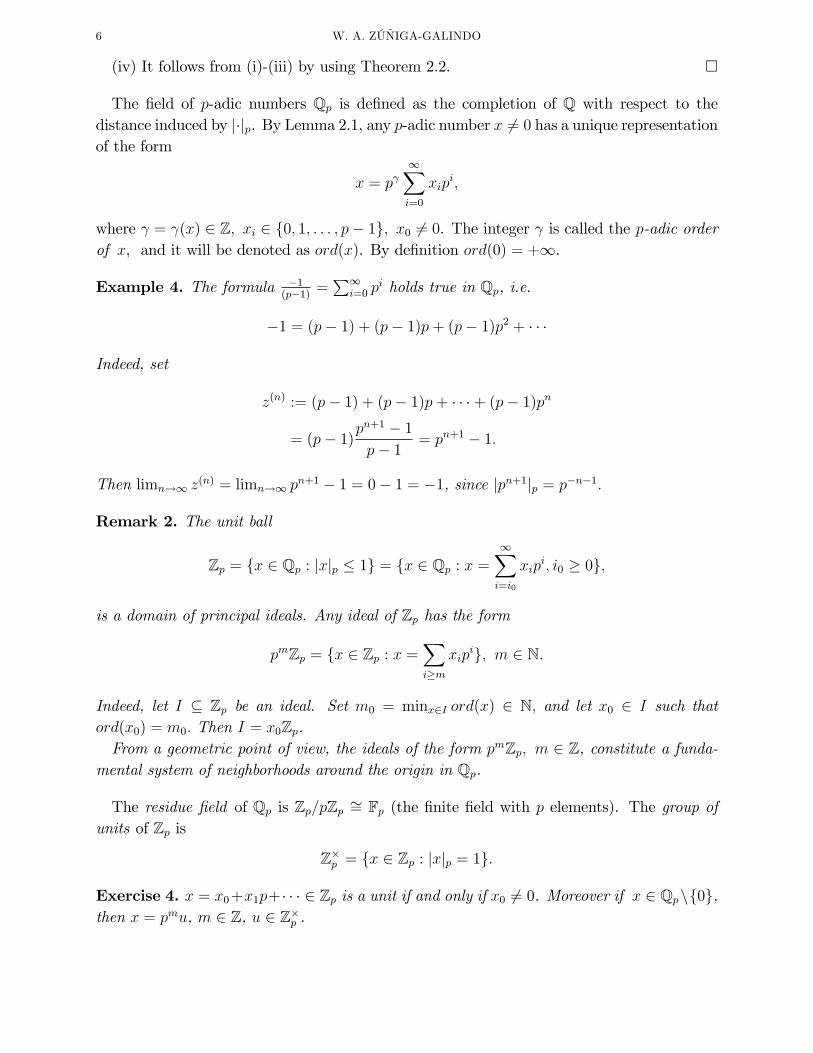
The �eld of p-adic numbers Qp is de�ned as the completion of Q with respect to thedistance induced by j�jp. By Lemma 2.1, any p-adic number x 6= 0 has a unique representationof the form

x = p 1Xi=0

xipi;

where = (x) 2 Z; xi 2 f0; 1; : : : ; p� 1g; x0 6= 0. The integer is called the p-adic orderof x, and it will be denoted as ord(x). By de�nition ord(0) = +1.

Example 4. The formula �1(p�1) =

P1i=0 p

i holds true in Qp, i.e.

�1 = (p� 1) + (p� 1)p+ (p� 1)p2 + � � �

Indeed, set

z(n) := (p� 1) + (p� 1)p+ � � �+ (p� 1)pn

= (p� 1)pn+1 � 1p� 1 = pn+1 � 1:

Then limn!1 z(n) = limn!1 p

n+1 � 1 = 0� 1 = �1, since jpn+1jp = p�n�1:

Remark 2. The unit ball

Zp = fx 2 Qp : jxjp � 1g = fx 2 Qp : x =1Xi=i0

xipi; i0 � 0g;

is a domain of principal ideals. Any ideal of Zp has the form

pmZp = fx 2 Zp : x =Xi�m

xipig; m 2 N:

Indeed, let I � Zp be an ideal. Set m0 = minx2I ord(x) 2 N; and let x0 2 I such thatord(x0) = m0: Then I = x0Zp.From a geometric point of view, the ideals of the form pmZp; m 2 Z, constitute a funda-

mental system of neighborhoods around the origin in Qp.

The residue �eld of Qp is Zp=pZp �= Fp (the �nite �eld with p elements). The group ofunits of Zp is

Z�p = fx 2 Zp : jxjp = 1g:

Exercise 4. x = x0+x1p+� � � 2 Zp is a unit if and only if x0 6= 0. Moreover if x 2 Qpnf0g,then x = pmu, m 2 Z, u 2 Z�p .


2.3. Topology of Qp. De�ne

Br(a) = fx 2 Qp : jx� ajp � prg; r 2 Z;

as the ball with center a and radius pr, and

Sr(a) = fx 2 Qp : jx� ajp = prg; r 2 Z

as the sphere with center a and radius pr.The topology of Qp is quite di¤erent from the usual topology of R. First of all, since

j � jp : Qp ! fpm : m 2 Zg [ f0g, the radii are always integer powers of p, for the sake ofbrevity we just use the power in the notation Br(a) and Sr(a). On the other hand, since thepowers of p and zero form a discrete set in R, in the de�nition of Br(a) and Sr(a) we canalways use ��. Indeed,

fx 2 Qp : jx� ajp < prg = fx 2 Qp : jx� ajp � pr�1g = Br�1(a) � Br(a):

Remark 3. Notice that Br(a) = a+ p�rZp and Sr(a) = a+ p�rZ�p .

We declare that the Br(a), r 2 Z, a 2 Qp, are open subsets. These sets form a basis forthe topology of Qp.

Proposition 2.1. Sr(a), Br(a) are open and closed sets in the topology of Qp.

Proof. We �rst show that Sr(a) is open. Notice that

Sr(a) =G

i2f1;:::;p�1g

a+ p�ri+ p�r+1Zp =G

i2f1;:::;p�1g

B(r�1)(a+ p�ri);

and consequently Sr(a) is an open set.In order to show that Sr(a) is closed, we take a sequence fxngn2N of points of Sr(a)

converging to ex0 2 Qp. We must show that ex0 2 Sr(a). Note that xn = a+ p�run, un 2 Z�p .Since fxngn2N is a Cauchy sequence, we have

jxn � xmjp = prjun � umjp ! 0, n, m!1,

thus fungn2N is also Cauchy, and since Qp is complete un ! eu0. Then xn ! a + p�reu0, soin order to conclude our proof we must verify that eu0 2 Z�p . Because um is arbitrarily closeto eu0, their p-adic expansions must agree up to a big power of p, hence eu0 2 Z�p .A similar argument shows that Br(a) is closed. �

Lemma 2.2. If b 2 Br(a) then Br(b) = Br(a), i.e. any point of the ball Br(a) is its center.

Proof. Let x 2 Br(b), then

jx� ajp = jx� b+ b� ajp � maxfjx� bjp; jb� ajpg � pr;

i.e. Br(b) � Br(a). Since a 2 Br(b) (i.e. jb� ajp = ja� bjp � pr), we can repeat the previousargument to show that Br(a) � Br(b). �

Exercise 5. Show that any to balls in Qp are either disjoint or one is contained in another.


Exercise 6. Show that the boundary of any ball is the empty set.

Theorem 2.3. [1, Sec. 1.8] A set K � Qp is compact if and only if it is closed and boundedin Qp.

2.4. The n�dimensional p-adic space. We extend the p-adic norm to Qnp by taking

jjxjjp := max1�i�d

jxijp; for x = (x1; : : : ; xn) 2 Qnp :

We de�ne ord(x) = min1�i�nford(xi)g, then jjxjjp = p�ord(x). The metric space�Qnp ; jj � jjp

�is

a separable complete ultrametric space (here, separable means that Qnp contains a countabledense subset, which is Qn ).For r 2 Z, denote by Bn

r (a) = fx 2 Qnp : jjx� ajjp � prg the ball of radius pr with centerat a = (a1; : : : ; an) 2 Qnp , and take Bn

r (0) := Bnr . Note that B

nr (a) = Br(a1)� � � � � Br(an),

where Br(ai) := fxi 2 Qp : jxi � aijp � prg is the one-dimensional ball of radius prwith center at ai 2 Qp. The ball Bn

0 equals the product of n copies of B0 = Zp. We alsodenote by Snr (a) = fx 2 Qnp : jjx � ajjp = prg the sphere of radius pr with center ata = (a1; : : : ; an) 2 Qnp , and take Snr (0) := Snr . We notice that S

10 = Z�p (the group of units

of Zp), but�Z�p�n ( Sn0 .

As a topological space�Qnp ; jj � jjp

�is totally disconnected, i.e. the only connected subsets

of Qnp are the empty set and the points. Two balls inQnp are either disjoint or one is containedin the other. As in the one dimensional case, a subset of Qnp is compact if and only if it isclosed and bounded in Qnp . Since the balls and spheres are both open and closed subsets inQnp , one has that

�Qnp ; jj � jjp

�is a locally compact topological space.

3. Integration on Qnp

3.1. Measure theory: a basic dictionary. The notion of measure of a set is a mathe-matical abstraction of the naive notions of length of a segment, the area of a plane �gure,and the volume of a body.Let X be a non-empty set. We want to introduce a notion of measure for a class of subsets

of X. A suitable class is a �-algebra of subsets of X. Denote by P(X) the power set of X,then a subset � � P(X) is called a �-algebra, if it satis�es the following properties:(i) X 2 �;(ii) � is closed under complementation: if A 2 � then Ac := X r A 2 �;(iii) � is closed under countable unions: if Ai 2 � for i 2 N, then [i2NAi 2 �.Notice that if follows from the above de�nition that ? 2 �, and that � is closed under

countable intersections. The elements of � are called measurable sets, which means that wecan assign a measure to these sets. The pair (X;�) is called a measurable space. Assumethat (Y;�) is another measurable space and that f : (X;�)! (Y;�) is a function betweenmeasurable spaces. The function f is called a measurable function if the preimage of everymeasurable set is measurable.

Example 5. Let X be a non-empty set. the following are some simple examples of �-algebras.


(i) � = fX;?g, this is the trivial �-algebra;(ii) � = P(X), this is the discrete �-algebra;(iii) � = fX;?; A;Acg is the �-algebra generated by the subset A.

Example 6. Let F be a family of subsets of X. Then there exists a unique smallest �-algebra� (F ) which contains any set in F . The �-algebra � (F ) is called the �-algebra generated byF , it agrees with intersection of all the �-algebras containing F . If (X; d) is a metric space,the �-algebra generated by the open balls is called the Borel �-algebra of X.

De�nition 8. Let (X;�) be a measurable space. A function � : � ! [0;+1] is called ameasure if it satis�es the following properties:(i) � (?) = 0;(ii) for any countable collection Ai, i 2 N, of pairwise disjoint sets in �,

�

�Fi2N

Ai

�=Xi2N

� (Ai) :

Let � be a measure on (X;�). The following are some basic properties of �:(i) monotonicity: if A1 and A2 are measurable sets with A1 � A2, then � (A1) � � (A2);(ii) subadditivity: for any countable collection Ai, i 2 N, of measurable sets in �,

�

[i2N

Ai

!�Xi2N

� (Ai) ;

(iii) continuity from below: if Ai, i 2 N, are measurable sets in � such that Ai � Ai+1 forall i, then the union of the sets Ai is measurable, and

�

[i2N

Ai

!= lim

i!1� (Ai) ;

(iv) continuity from above: if Ai, i 2 N, are measurable sets in � such that Ai+1 � Ai for alli, then the intersection of the sets Ai is measurable. In addition, if A0 has �nite measure,then

�

\i2N

Ai

!= lim

i!1� (Ai) .

3.2. The Haar measure.

Theorem 3.1. [9, Thm B. Sec. 58] Let (G; �) be a locally compact topological, Abeliangroup. There exists a regular Borel measure �Haar (called a Haar measure of G), unique upto multiplication by a positive constant, such that �Haar (U) > 0 for every non empty Borelopen set U , and �Haar (x � E) = �Haar (E), for every Borel set E.

Notation 1. We will denote the Haar measure by dx, then �Haar (U) =RUdx.

Exercise 7. Prove that (Qp;+), respectively (Q�p ; �), are locally compact topological groups.Since Qp, respectively Q�p = Qpnf0g, are metric spaces, the continuity of the sum, respectively


of the product, means that if xn ! x; and yn ! y, then xn + yn ! x + y, respectivelyxnyn ! xy:

Since (Qp;+) is a locally compact topological group, by Theorem 3.1 there exists a measuredx, which is invariant under translations, i.e. d(x + a) = dx. If we normalize this measureby the condition

RZp dx = 1, then dx is unique.

In the n-dimensional case, (Qnp ;+) is also locally compact topological group. We denoteby dnx the Haar measure normalized by the condition

RZnpdnx = 1. This measure agrees

with the product measure dx1 � � � dxn, and it also satis�es that dn(x+ a) = dnx, for a 2 Qnp .The open compact balls of Qnp , e.g. a + pmZnp ; generate the Borel �-algebra of Qnp . The

measure dnx assigns to each open compact subset U a nonnegative real numberRUdnx,

which satis�es

(3.1)Z[1k=1Uk

dnx =1Xk=1

ZUk

dnx;

for all compact open subsets Uk in Qnp , which are pairwise disjoint, and verify [1k=1Uk is stillcompact. In addition, Z

a+U

dnx =

ZU

dnx:

Remark 4. Let B(Qnp ) be the Borel �-algebra on Qnp . Let dnx be the normalized Haar

measure on�Qnp ;B(Qnp )

�. The Haar measure of a Borel set A is denoted as �(n)Haar(A). The

fact that dnx is a regular measure means that for any measurable subset A of Qnp is holdsthat

�(n)Haar(A)= sup

n�(n)Haar (F ) : F � A, F compact and measurable

o= inf

n�(n)Haar(G) : G � A, G open and measurable

o:

3.3. Integration of locally constant functions. A function ' : Qnp ! C is said to belocally constant if for every x 2 Qnp there exists an open compact subset U , containing x,and such that f(x) = f(u) for all u 2 U .

Exercise 8. Every locally constant function is continuous.

Any locally constant function ' : Qnp ! C can be expressed as a linear combination ofcharacteristic functions of the form

(3.2) ' (x) =

1Xn=1

ck1Uk (x) ;

where ck 2 C,

1Uk (x) =

8><>:1 if x 2 Uk

0 if x =2 Uk;


and Uk � Qnp is an open compact for every k. Indeed, there exists a covering fUigi2N of Qnpsuch that each Ui is open compact and ' jUi is a constant function. Since

�Qnp ; k�kp

�is a

separable metric space any open cover has a countable subcover, consequently we may takeN = N.Let ' : Qnp ! C be a locally constant function as in (3.2). Assume that A =

Fki=1 Ui, the

symbolFmeans disjoint union, i.e. the sets Ui are pairwise disjoint, with Ui open compact.

Then, we de�ne

(3.3)ZA

' (x) dnx = c1

ZU1

dnx+ � � �+ cn

ZUk

dnx:

We recall that given a function ' : Qnp ! C the support of ' is the set

Supp(') = fx 2 Qnp : '(x) 6= 0g:

A locally constant function with compact support is called a test function or a Bruhat-Schwartz function. These functions form a C-vector space denoted as D := D

�Qnp�. From

(3.1) and (3.3) one has that the mapping

(3.4)D �! C' 7�!

RQnp' dnx;

is a well-de�ned linear functional.

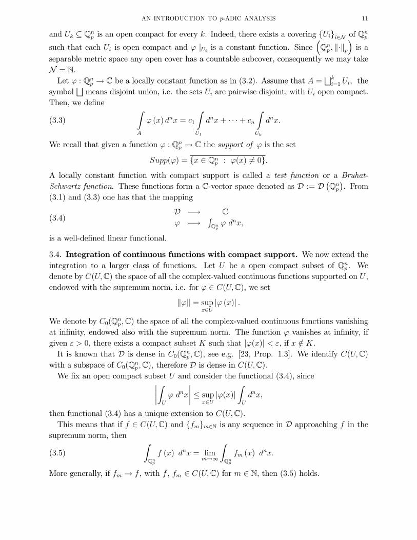
3.4. Integration of continuous functions with compact support. We now extend theintegration to a larger class of functions. Let U be a open compact subset of Qnp . Wedenote by C(U;C) the space of all the complex-valued continuous functions supported on U ,endowed with the supremum norm, i.e. for ' 2 C(U;C), we set

k'k = supx2U

j' (x)j :

We denote by C0(Qnp ;C) the space of all the complex-valued continuous functions vanishingat in�nity, endowed also with the supremum norm. The function ' vanishes at in�nity, ifgiven " > 0, there exists a compact subset K such that j'(x)j < ", if x =2 K.It is known that D is dense in C0(Qnp ;C), see e.g. [23, Prop. 1.3]. We identify C(U;C)

with a subspace of C0(Qnp ;C), therefore D is dense in C(U;C).We �x an open compact subset U and consider the functional (3.4), since��Z

U

' dnx

�� supx2U

j'(x)jZU

dnx;

then functional (3.4) has a unique extension to C(U;C).This means that if f 2 C(U;C) and ffmgm2N is any sequence in D approaching f in the

supremum norm, then

(3.5)ZQnpf (x) dnx = lim

m!1

ZQnpfm (x) d

nx:

More generally, if fm ! f , with f , fm 2 C(U;C) for m 2 N, then (3.5) holds.


3.4.1. Some remarks on uniform convergence. We recall the notion of uniform convergence.Let E be a non-empty set. Let fn : E ! C, n 2 N be a sequence of complex-valued functions.We say that the sequence ffng n2N is uniformly convergent on E with limit f : E !C, iffor every � > 0, there exists a natural number N such that for all n > N and any x 2 E,jfn(x)� f(x)j < �, which is equivalent to say for every � > 0, there exists a natural numberN such that for all n > N , supx2E jfn(x)� f(x)j < �.The Weierstrass M-test is a very useful criterion for determining the uniform convergence

of sequences. Let ffng n2N be a sequence of functions fn : E ! C and let Mn be a sequenceof positive real numbers such that jfn(x)j < Mn for all x 2 E and n 2 N. If

PnMn

converges, thenP

n fn converges uniformly on E.

3.4.2. Some remarks on convergent power series. Let us denote by C [[z1; : : : ; zn]], the ringof formal power series with coe¢ cients in C. An element of this ring has the formPi

cizi =

P(i1;:::;in)2Nn

ci1;:::;inzi11 : : : z

inn , where i = (i1; : : : ; in) 2 Nn, and the ci1;:::;ins are in C.

A formal seriesP

i cizi is said to be convergent if there exists a positive real number R

such thatP

i ciai converges for any a = (a1; : : : ; an) 2 Cn satisfying maxi jaij < R. The

convergent series form a subring of C [[x1; : : : ; xn]], which will be denoted as C hhx1; : : : ; xnii.If for

Pi ciz

i there existsP

i c(0)i xi 2 R hhx1; : : : ; xnii (a real convergent series) such that

jcij � c(0)i for all i 2 Nn, we say that

Pi c(0)i xi is a dominant series for

Pi cix

i and writePcix

i <<Pc(0)i xi:

Exercise 9. A formal power series is convergent if and only if it has a dominant series.

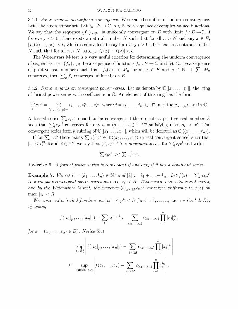
Example 7. We set k = (k1; : : : ; kn) 2 Nn and jkj := k1 + : : : + kn. Let f(z) =P

k ckzk

be a complex convergent power series on maxi jzij < R. This series has a dominant series,and by the Weierstrass M-test, the sequence

Pjkj�M ckz

k converges uniformly to f(z) onmaxi jzij < R.We construct a �radial function�on jxijp � pL < R for i = 1; : : : ; n, i.e. on the ball Bn

L,by taking

f(jx1jp ; : : : ; jxnjp) =Xk

ck jxjkp :=X

(k1;:::;kn)

c(k1;:::;kn)

nYi=1

jxijkip ;

for x = (x1; : : : ; xn) 2 BnL. Notice that

supx2BnL

��f(jx1jp ; : : : ; jxnjp)�Xjkj�M

c(k1;:::;kn)

nYi=1

jxijkip

�� sup

maxijzij<R

��f(z1; : : : ; zn)�Xjkj�M

c(k1;:::;kn)

nYi=1

zkii

�� ;


and consequentlyP

jkj�M c(k1;:::;kn)nQi=1

jxijkip converges uniformly to f(jx1jp ; : : : ; jxnjp) on BnL.

Then ZBnL

f(jx1jp ; : : : ; jxnjp)dnx = limM!1

Xjkj�M

c(k1;:::;kn)

ZBnL

nYi=1

jxijkip dnx

= limM!1

Xjkj�M

c(k1;:::;kn)

nYi=1

ZBL

jxijkip dxi:(3.6)

3.5. The change of variables formula in dimension one. Let us start by establishingthe formula:

(3.7) d (ax) = jajp dx, a 2 Q�p ;

which means the following: ZaU

dx = jajpZU

dx;

for every Borel set U � Qp, for instance an open compact subset. Indeed, consider

Ta : Qp �! Qp

x 7�! ax;

with a 2 Q�p . Ta is a topological and algebraic isomorphism. Then U 7!RaUdx is a Haar

measure for (Qp;+), and by the uniqueness of such measure, there exists a positive constantC(a) such that

RaUdx = C(a)

RUdx. To compute C(a) we can pick any open compact set,

for instance U = Zp, and then we must showRaZp dx = C(a) = jajp :

Let us consider �rst the case a 2 Zp, i.e. a = plu, l 2 N, u 2 Z�p . Fix a system ofrepresentatives fbg of Zp=plZp in Zp, then

Zp =F

b2Zp=plZpb+ plZp;

and

1 =RZpdx =

Pb2Zp=plZp

Rb+plZp

dx =P

b2Zp=plZp

RplZp

dx

= #�Zp=plZp

� RplZp

dx;

i.e.

p�l = jajp =RplZp

dx =

ZaZp

dx:

The case a =2 Zp is treated in a similar way.


Now, if we take f : U ! C, where U is a Borel set, thenRU

f (x) dx = jajpR

a�1U�a�1bf (ay + b) dy; for any a 2 Q�p ; b 2 Qp:

The formula follows by changing variables as x = ay + b. Then we get dx = d (ay + b) =

d(ay) = jajp dy, because the Haar measure is invariant under translations and formula (3.7).

Example 8. For any r 2 Z, RBr

dx =R

p�rZpdx = pr

RZpdy = pr.

Example 9. For any r 2 Z,RSr

dx =RBr

dx�R

Br�1

dx = pr � pr�1 = pr�1� p�1

�.

Example 10. Take U = Zp r f0g. We show thatRU

dx =RZpdx = 1:

Notice that U is not compact, since the sequence fpngn2N � U converges to 0 =2 U . Now, byusing

Zp r f0g =1Fj=0

nx 2 Zp : jxjp = p�j

o;

we haveRZprf0g

dx =1Pj=0

RpjZ�p

dx (by changing variables as x = pjy, dx = p�jdy)

=

1Pj=0

p�j

! RZ�p

dy =1� p�1

1� p�1= 1:

This calculation shows that Zpr f0g has Haar measure 1 and that f0g has Haar measure 0.

Example 11. Set

Z(s) :=R

Zprf0gjxjsp dx, s 2 C with Re(s) > �1:

We prove that Z(s) has a meromorphic continuation to the whole complex plane as a rationalfunction of p�s.Indeed,

Z(s) =R

Zprf0gjxjsp dx =

1Pj=0

Rjxjp=p�j

jxjsp dx =1Pj=0

p�jsR

jxjp=p�jdx

=�1� p�1

� 1Pj=0

p�j(s+1) (here we need the hypothesis Re(s) > �1)

=(1� p�1)

1� p�1�s; for Re(s) > �1.


We now note that the right hand-side is de�ned for any complex number Re(s) 6= �1, there-fore, it gives a meromorphic continuation of Z(s) to the half-plane Re(s) < �1. Thus, wehave shown that Z(s) has a meromorphic continuation to the whole C with a simple pole atRe(s) = �1.

Example 12. We compute

Z(s; x2 � 1) =RZp

��x2 � 1��spdx; for Re(s) > �1, p 6= 2.

Let us take f0; 1; : : : ; p� 1g � Z � Zp as a system of representatives of Fp ' Zp=pZp.Then

Zp =p�1Fj=0

(j + pZp);

and

Z(s; x2 � 1) =p�1Pj=0

Rj+pZp

j(x� 1) (x+ 1)jsp dx

= p�1p�1Pj=0

RZpj(j � 1 + py) (j + 1 + py)jsp dy; (x = j + py).

Let us consider �rst the integrals in which j� 1+ py 2 Z�p , i.e. the reduction mod p of j� 1is a nonzero element of Fp, in this caseR

Zpj(j � 1 + py) (j + 1 + py)jsp dy = 1;

and since p 6= 2 there are exactly p� 2 of those j�s, then

Z(s; x2 � 1) = (p� 2) p�1 + p�1RZpjpy (2 + py)jsp dy + p�1

RZpj(�2 + py) pyjsp dy

= (p� 2) p�1 + 2p�1�sRZpjyjsp dy = (p� 2) p�1 + 2p�1�s

1� p�1

1� p�1�s:

Exercise 10. Take q (x) =rQi=1

(x� �i)ei 2 Zp [x], �i 2 Zp, ei 2 N r f0g. Assume that

�i 6� �j mod p. By using the methods presented in examples 11 and 12 compute the integral

Z(s; q(x)) =RZpjq (x)jsp dx:

3.6. Improper Integrals. Our next task is the integration of functions that do not havecompact support. A function f : Qnp ! C is said to be locally integrable, f 2 L1loc, ifZ

K

f (x) dnx

exists for every compact subset K.


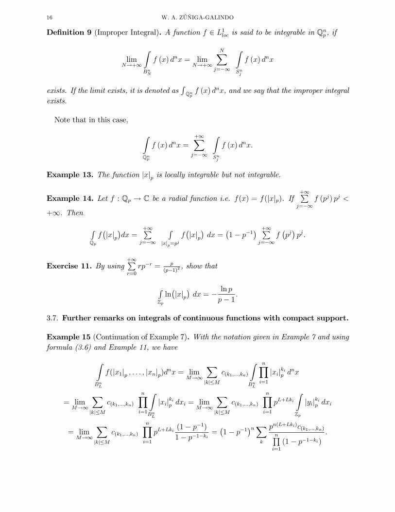
De�nition 9 (Improper Integral). A function f 2 L1loc is said to be integrable in Qnp , if

limN!+1

ZBnN

f (x) dnx = limN!+1

NXj=�1

ZSnj

f (x) dnx

exists. If the limit exists, it is denoted asRQnpf (x) dnx, and we say that the improper integral

exists.

Note that in this case,

ZQnp

f (x) dnx =

+1Xj=�1

ZSnj

f (x) dnx:

Example 13. The function jxjp is locally integrable but not integrable.

Example 14. Let f : Qp ! C be a radial function i.e. f(x) = f(jxjp). If+1Pj=�1

f (pj) pj <

+1. Then

RQpf�jxjp�dx =

+1Pj=�1

Rjxjp=pj

f�jxjp�dx =

�1� p�1

� +1Pj=�1

f�pj�pj.

Exercise 11. By using+1Pr=0

rp�r = p

(p�1)2 , show that

RZpln�jxjp�dx = � ln p

p� 1 :

3.7. Further remarks on integrals of continuous functions with compact support.

Example 15 (Continuation of Example 7). With the notation given in Example 7 and usingformula (3.6) and Example 11, we haveZ

BnL

f(jx1jp ; : : : ; jxnjp)dnx = limM!1

Xjkj�M

c(k1;:::;kn)

ZBnL

nYi=1

jxijkip dnx

= limM!1

Xjkj�M

c(k1;:::;kn)

nYi=1

ZBnL

jxijkip dxi = limM!1

Xjkj�M

c(k1;:::;kn)

nYi=1

pL+LkiZZp

jyijkip dxi

= limM!1

Xjkj�M

c(k1;:::;kn)

nYi=1

pL+Lki(1� p�1)

1� p�1�ki=�1� p�1

�nXk

pn(L+Lki)c(k1;:::;kn)nQi=1

(1� p�1�ki):


Example 16. Let f(x) = e�jxjp�jxjp�, where

�jxjp�denotes the characteristic function

of Zp. We compute �rstRf(x)dx by using Example 14:Z

Qpe�jxjp

�jxjp�dx =

ZZpe�jxjpdx =

1Xj=0

ZpjZ�p

e�jxjpdx

=

1Xj=0

e�p�jZpjZ�p

dx =

+1Xj=0

p�j�1� p�1

�e�p

�j:

We now compute the integral by using Example 15:ZZpe�jxjpdx = lim

M!1

MXk=0

(�1)k

k!

ZZpjxjkp dx =

�1� p�1

� 1Xk=0

(�1)k

k! (1� p�1�k):

Consequently,1Xj=0

p�j�1� p�1

�e�p

�j=�1� p�1

� 1Xk=0

(�1)k

k! (1� p�1�k):

We invite the reader to verify this identity directly .

4. Change of variables formula

A function h : U ! Qp is said to be analytic on an open subset U � Qnp , if for everyb = (b1; : : : ; bn) 2 U there exists an open subset eU � U , with b 2 eU , and a convergentpower series

Pi2Nn ai (x� b)i for x = (x1; : : : ; xn) 2 eU , such that h (x) = Pi2Nn ai (x� b)i

for x 2 eU , with i = (i1; : : : ; in) and (x� b)i =Qnj=1 (xj � bj)

ij . In this case, @@xlh (x) =P

i2Nn ai@@xl(x� b)i is a convergent power series.

Let U , V open subsets in Qnp . A mapping H : U ! V , H = (H1; : : : ; Hn) is called analyticif each Hi is analytic. The mapping H is said to be bi-analytic if H and H�1 are analytic.

Theorem 4.1. Let K0; K1 � Qnp be open compact subsets, and let H = (H1; : : : ; Hn) : K1 !K0 be a bi-analytic map such that

det

�@Hi

@yj(z)

�6= 0, for any z 2 K1:

If f is a continuous function on K0, thenRK0

f (x) dnx =RK1

f (�(y))

��det �@Hi

@yj(y)

��p

dny; (x = H(y)).

For the proof of this theorem the reader may consult [10, Prop. 7.4.1] or [8, Section 10.1.2].

Example 17. Set U := Qp r��dc

and V := Qp r

�ac

, where a, b, c, d 2 Qp, with c 6= 0.

Consider the functionU ! V

x ! y = ax+bcx+d

;


this is an analytic function in U , with inverse x = dy�b�cy+a , which is analytic in V . Assume

that ad � bc 6= 0, and take ' : Qp ! C a Bruhat-Schwartz function with support containedin V , then Z

V

' (y) dy =

ZU

'

�ax+ b

cx+ d

� jad� bcjpjcx+ dj2p

dx:

Example 18. ComputeRBnrdnx, where Bn

r =nx 2 Qnp : kxkp � pr

o. We �rst recall that

Bnr = p�rZnp =

p�rZp � : : :� p�rZpn� copies| {z } :

By changing variables as xi = p�ryi for i = 1; : : : ; n, we have dnx = pnrdny, andZBnr

dnx = pnrZZnpdnx = pnr.

Exercise 12. Show that ZSnr

dnx = pnr�1� p�1

�:

Exercise 13. To generalize Example 11 to Qnp , i.e. to show that the integral

Z(s) =

ZZnprf0g

kxksp dnx, for Re(s) > 0,

admits an analytic continuation to the whole complex plane as a rational function of p�s.

Exercise 14. Let � be a real number. To show that

I (�) =

ZZnprf0g

1

kxk�pdnx <1 if � < n.

Exercise 15. Let � be a real number. To show that

J (�) =

ZQnprZnp

1

kxk�pdnx <1 if � > n.

Example 19. Take N � 4 and complex variables s1j and s(N�1)j for 2 � j � N � 2 and sijfor 2 � i < j � N � 2. Put s := (sij) 2 Cd, where d = N(N�3)

2denotes the total number of

indices ij. The Koba-Nielsen local zeta functions is de�ned as follows:

Z(N) (s) =

ZQN�3p

N�2Yi=2

jxjjs1jp j1� xjjs(N�1)jp

Y2�i<j�N�2

jxi � xjjsijpN�2Yi=2

dxi;

whereQN�2i=2 dxi is the normalized Haar measure on QN�3p . If N = 4, we have

(4.1) Z(4) (s) =

ZQp

jxjs12p j1� xjs32p dx.


Notice that in integral (4.1) does not contain a test function, and consequently its convergenceis not direct. In order to regularize it, we proceed as follows:

Z(4) (s12; s32) =

ZZp

jxjs12p j1� xjs32p dx+

ZQprZp

jxjs12p j1� xjs32p dx

= : Z(4)0 (s12; s32) + Z

(4)1 (s12; s32) :

To study integral Z(4)0 (s12; s32), we use that Zp =Fp�1j=0 j + pZp, to get

Z(4)0 (s12; s32) =

p�1Pj=0

Zj+pZp

jxjs12p j1� xjs32p dx =:p�1Pj=0

Z(4)0;j (s12; s32) :

Now, for j 6= 0; 1,Z(4)0;j (s12; s32) = p�1:

In the case j = 0,

Z(4)0;0 (s12; s32) =

ZpZp

jxjs12p dx = p�1�s12�

1� p�1

1� p�1�s12

�:

In the case j = 1,

Z(4)0;1 (s12; s32) =

Z1+pZp

j1� xjs32p dx = p�1�s32ZZp

jyjs32p dy

= p�1�s32�

1� p�1

1� p�1�s32

�:

Consequently,

Z(4)0 (s12; s32) = (p� 2) p�1 + p�1�s32

�1� p�1

1� p�1�s32

�+ p�1�s32

�1� p�1

1� p�1�s32

�:

Notice that Z(4)0 (s12; s32) is holomorphic, and consequently the underlying integrals converge,in

(4.2) Re (s12) > �1 and Re(s32) > �1:

To study Z(4)1 (s12; s32), we �rst notice that

Z(4)1 (s12; s32) =

ZQprZp

jxjs12p j1� xjs32p dx =

ZQprZp

jxjs12+s32p dx:

Now, we use the change of variables:

x =1

y, dx =

dy

jyj2p;


then

Z(4)1 (s12; s32) =

ZQprZp

jxjs12+s32p dx =

ZpZp

jyj�2�s12�s32p dy

= p�1+2+s12+s32ZZp

jyj�2�s12�s32p dy = p�1+2+s12+s32�

1� p�1

1� ps12+s32+1

�:

Thus Z(4)1 (s12; s32) is holomorphic in

(4.3) Re(s12) + Re (s32) + 1 < 0:

Finally, it is not di¢ cult to see that conditions (4.2)-(4.3) de�ne an open set in C.The calculation presented in this example still requires some additional work, since it

involves non compact subsets. The �missing� part can be obtained easily by applying thedominated convergence theorem.

5. Additive characters

Given a nonzero p-adic number

x = x�mp�m + x�m+1p

�m+1 + : : :+ x�1p�1 + x0 + xp+ : : : with x�m 6= 0 and m > 0;

we de�ne its fractional part as

fxgp = x�mp�m + x�m+1p

�m+1 + : : :+ x�1p�1 2 Q.

If x 2 Zp, we set fxgp := 0. Now the function

�p (x) := exp 2�i fxgpis called the standard additive character of Qp (more precisely of (Qp;+)). Notice that

�p : (Qp;+)! (S; �)

is a continuous homomorphism from (Qp;+) into the unit complex circle considered as amultiplicative group, i.e. �p satis�es the following:(i)��p (x)�� = 1 for x 2 Qp;

(ii) �p (x+ y) = �p (x)�p (y) for x, y 2 Qp;(iii) �p (x) =

1�p(x)

= �p (�x) for x 2 Qp, where the bar means complex conjugate;(iv) �p (x) 6� 1 for x 2 Qp r Zp.

Example 20. Let r be an integer. To show thatZBr

�p (�x) dx =

8><>:pr if j�jp � p�r

0 if j�jp � p�r+1:

If j�jp � p�r, then j�xjp � 1 which means that �x 2 Zp and thus �p (�x) � 1,ZBr

�p (�x) dx =

ZBr

dx = pr:


If j�jp � p�r+1, there exists x0 2 Sr, i.e. jx0jp = pr, such that jx0�jp � p, i.e. x0� 2 Qp rZpand thus we may assumee that �p (x0�) 6� 1. We now change variables as x = y+x0, noticethat y runs through p�rZp, to get

�p (�x0)

Zjyjp�pr

�p (�y) dy =

Zjxjp�pr

�p (�x) dx;

which implies the announced formula.

Exercise 16. Let r be an integer. For x = (x1; : : : ; xn), � = (�1; : : : ; �n) 2 Qnp , we setx � � :=

Pi xi�i. To show thatZ

Bnr

�p (x � �) dnx =

8><>:prn if k�kp � p�nr

0 if k�kp � p�nr+1:

Hint: remenber that x = pord(x)ex, with kexkp = 1 and � = pord(�)e�, with e� p= 1. Thus

x � � = pord(x)+ord(�)ex � e�.Exercise 17. Let r be an integer. To show that

ZSr

�p (�x) dx =

8>>>>><>>>>>:

pr (1� p�1) if j�jp � p�r

�pr�1 if j�jp = p�r+1

0 if j�jp � p�r+2:

Hint: use Example 20 andZSr

�p (�x) dx =

ZBr

�p (�x) dx�ZBr�1

�p (�x) dx:

Exercise 18. Extend the formula given in Example 14 to n-dimensional case, i.e. for radialfunctions f : Qnp ! C i.e. f(x) = f(kxkp).

Exercise 19. Let f : R! C be a function such that1Pr=0

jf (p�r)j p�r < +1. Then

ZQp

f�jxjp��p (�x) dx =

(1� p�1)

j�jp

1Xr=0

f

p�r

j�jp

!p�r � 1

j�jpf

p

j�jp

!for � 6= 0,

in the sense of improper integrals.

By using this exercise with f � 1, we get thatZQp

�p (�x) dx =

8><>:1 if � = 0

0 if � 6= 0= � (�) , the Dirac distribution.

Which is the Fourier transform of the constant function 1 is the Dirac distribution (or Diracdelta function).


6. Fourier Analysis on Qnp

6.1. Some function spaces. For 1 � � < 1, we denote by L� := L��Qnp ; dnx

�, the

C-vector space of all the complex-valued and Borel measurable functions f satisfying

kfk� :=

8><>:ZQnp

jf (x)j� dnx

9>=>;1�

<1.

For � =1, f 2 L1 := L1�Qnp ; dnx

�, if

(6.1) kfk1 := ess supx2Qnp jf (x)j <1.

The condition appearing on the right-hand side in (6.1) means that function f is boundedalmost everywhere, i.e. this condition may be false in a set of measure zero. L� is a Banachspace if we identify functions f and g satisfying f(x) = g(x) almost everywhere. This meansthat k�k� is norm, that that L� is a complete metric space for the distance induced by k�k�.We denote by C0 := C0(Qnp ;C) the C-vector space of continuous functions on Qnp that

vanish at in�nity endowed with the L1-norm. The condition �vanish at in�nity�means thatfor any � > 0 there exists a compact subset K � Qnp such that

jf (x)j < � for x 2 Qnp rK.

Remark 5. Lebesgue�s dominated convergence theorem. Let fm : Qnp ! C, m 2 N, bea sequence of complex-valued Borel measurable functions. Suppose that the sequence con-verges pointwise to a function f and that there exists an integrable function g such thatjfm(x)j � g(x) for any x 2 Qnp and all m, then f is integrable and

limm!1

ZQnpfm (x) d

nx =

ZQnplimm!1

fm (x) dnx =

ZQnpf (x)dnx:

6.2. The Fourier transform. Given x = (x1; : : : ; xn) 2 Qnp and � = (�1; : : : ; �n) 2 Qnp , wede�ne

x � � = x1�1 + : : :+ xn�n:

If f 2 L1 its Fourier transform is the function bf de�ned bybf (�) = Z

Qnp

f (x)�p (x � �) dnx:

We also use the notation Fx!� (f), F (f) to denote the Fourier transform of f .

Lemma 6.1. (i) The mapping f ! bf is a bounded linear mapping from L1 to L1 satisfying bf 1� kfk1.

(ii) If f 2 L1, then bf is uniformly continuous.


Proof. (i) �� bf (�)�� =��ZQnp

f (x)�p (x � �) dnx

�� ZQnp

jf (x)j dnx = kfk1 :

(ii) Notice that

bf (� + h)� bf (�) = ZQnp

f (x)�p (x � �)��p (x � h)� 1

dnx;

and since��f (x)�p (x � �)��p (x � h)� 1�� 2 jf (x)j 2 L1, by using the dominated conver-

gence theorem,

limh!0

�� bf (� + h)� bf (�)�� ZQnp

jf (x)j limh!0

��p (x � h)� 1�� dnx = 0;i.e. for any � > 0, there is � > 0, such that for any �0, � 2 Qnp , with k�0 � �kp = khkp < �, it

holds that�� bf (�0)� bf (�)�� < �. �

Remark 6. The translation operator Th, h 2 Qnp , is de�ned by (Thf) (x) = f (x� h). If f 2L1, then\(Thf) (�) = �p (� � h) bf (�), and Fx!�(�p (x � h) f (x)) = �T�h bf� (�) = bf (� + h).

We denote by �k (x) := �p�k kxkp

�the characteristic function of the ball Bn

k = p�kZnpfor k 2 Z. A locally constant function with compact support (a test function) ' : Qnp ! Cis a linear combination of characteristic functions of balls, then

' (x) =mXi=1

ciThi�ki (x) :

Notice that Thi�ki (x) is the characteristic function of the ball hi + p�kiZnp . We denote byD(Qnp ) the C�vector space of test functions (the Bruhat-Schwartz).We set �k (x) = pkn

�pk kxkp

�for k 2 Z. Notice that �k satis�esZ

Qnp�k (x) d

nx = 1 for any k 2 Zp:

Exercise 20. To show that b�k (�) = �k (�). Hence if ' (x) =Pm

i=1 ciThi�ki (x) is a testfunction, then b' (�) =Pm

i=1 ci�p (� � h) �k (�). Consequently, b' (�) is also a test function.Remark 7. Notice that limk!1�k (x) = 1, and that

limk!1

�k (x) =

8><>:1 if x = 0

0 if x 6= 0:

Exercise 21. Set ht (�) :=RQp �p (�x) e

�tjxj�p dx, for t > 0, � > 0. Show that ht (�) is acontinuous function in x for t > 0 �xed.


Proposition 6.1 ([23, Chap. I, Proposition 1.3]). D(Qnp ) is dense in C0 as well as in L�,1 � � <1.

Proposition 6.2 (Riemann-Lebesgue Theorem). If f 2 L1, then bf (�)! 0 as k�kp !1.

Proof. For g 2 D(Qnp ), bg has compact support. Fix � > 0, then there exists g� 2 D(Qnp ) suchthat kf � g�k1 < �, cf. Proposition 6.1. For � =2supp bg� we have�� bf (�)�� = �� bf (�)� bg� (�)�� \(f � g�)

1� kf � g�k1 < �:

�

De�nition 10. Given f , g : Qnp ! C its convolution is the function

h(x) = f(x) � g(x) =ZQnpf(x� z)g(z)dnz

=

ZQnpf(z)g(x� z)dnz;

when the de�ning integral exists.

Remark 8. Young�s inequality. Assume that f 2 L�, g 2 L� and 1�+ 1

�= 1

+ 1 with

1 � �; �; � 1. Then kf � gk � kfk� kgk�.

The following proposition is left as an exercise to the reader.

Proposition 6.3. If f 2 L�, 1 � � � 1, and g 2 L1, then f � g 2 L� and kf � gk� �kfk� kgk1.

Remark 9. Fubini�s theorem. Let f : Qn+mp ! C be a function such that the repeatedintegral Z

Qnp

ZQmp

f(x; y)dmy

!dnx

exists, then f 2 L1�Qn+mp ; dn+mx

�, and the following formulae hold:Z

Qnp

ZQmp

f(x; y)dmy

!dnx =

ZQn+mp

f(x; y)dnxdmy

=

ZQmp

ZQnpf(x; y)dnx

!dmy:

Lemma 6.2. If f , g 2 L1, then [f � g = bf bg.Proof. By Proposition 6.3 f � g 2 L1. The formula for the Fourier transform follows fromFubini�s theorem. We invite the redear to verify this calculation. �

Lemma 6.3. If f , g 2 L1, thenZQnp

bf(y)g (y) dny = ZQnpf(x)bg (x) dny:


Proof. By Fubini�s theorem and the de�nition of Fourier transform:ZQnp

bf(y)g (y) dny =

ZQnp

(ZQnp�p (x � y) f (x) dnx

)g (y) dny

ZQnp

(ZQnp�p (x � y) g (y) dny

)f (x) dnx =

ZQnpf(x)bg (x) dnx:

�

6.3. The Fourier transform on the space of test functions. Let ' : Qnp ! C be alocally constant function, this means that for each x 2 Qnp , there exists an integer l = l(x)

such that

(6.2) '(x+ x0) = '(x) for any x0 2 Bnl :

Since Bnl =

nx 2 Qnp : kxkp � pl

o= p�lZnp , condition (6.2) is equivalent to

' jx+p�lZnp� ' (x) :

If ' is a test function, then supp ' is open compact, and consequently there exist a �nitenumber of integers li and a �nite number of points zi in Qnp such that

supp ' =rFi=1

zi + p�liZnp :

We setk := max

1�i�r�li:

Then zi + p�liZnp � zi + pkZnp (i.e. Bn�k (zi) � Bn

li(zi)) and

' jx+pkZnp� ' (x) for any x 2 supp '.

This means that ' is constant on the cosets of pkZnp (i.e. on the cosets of Qnp=pkZnp). Wenow use the fact that supp ' is compact, which means that it is closed and bounded, thenthere exists an integer m such that

supp ' � pmZnp :

Naturally, for any x 2supp ', x+ pkZnp � pmZnp , which implies that k � m.In conclusion, ' 2 D(Qnp ) if and only there exist integers k, m, with k � m, such that

' is constant on the cosets of pkZnp (i.e. on the cosets of pmZnp=pkZnp) and is supportedon pmZnp . These functions form C-vector space denoted as Dmk (Qnp ) := Dmk . We �x a setof representatives Is of pmZnp=pkZnp =: Gm;n, then the characteristic functions of the ballsI + pkZnp , I 2 Gm;n span Dmk , i.e.n

�pk kx� Ikp

�oI2Gm;k

are a basis for Dmk . Notice that the dimension of Dmk is #Gm;k = p(m�k)n.

Lemma 6.4. F(Dmk ) � D�k�m.


Proof. Take ' 2 Dmk , since ' (x) =P

I2Gm;k cI�pk kx� Ikp

�, and F is a linear operator,

we may assume that ' (x) = �pk kx� Ikp

�. Then

Fx!��pk kx� Ikp

��=

RI+pkZnp

�p (� � x) dx = p�nk�p (� � I)RZnp�p�pk� � y

�dy

= p�nk�p (� � I) �p�k k�kp

�:

Finally, we verify that if k�0kp � p�m, then

�p (� � I) j�0+pmZnp= �p (�0 � I) ;

and consequently p�nk�p (� � I) � pk�

p

�2 D�k�m. �

Exercise 22. Show the following assertion. The map

(6.3)D(Qnp ) ! D(Qnp )

' ! b';where b' (�) = RQnp �p (� � x)' (x) dx, is a well-de�ned linear operator, with inverse given by

' (x) =

ZQnp�p (�� x) b' (�) d�:

In other words, the mapping (6.3) is a isomorphism of C-vector spaces on D(Qnp ).

6.4. The inverse Fourier transform. One expects that the inverse Fourier transform begiven by

f (x) =

ZQnp�p (�� x) bf (�) dn� = Z

Qnp�p (� � x) bf (�) dn�:

This formula does not always make sense since bf is not L1 when f 2 L1.Exercise 23. Show that the Fourier transform of f(x) =

�jxjp�ln�

1jxjp

�is

bf (�) =8><>:0 if j�jp � 1�ln p

1�p�1

�j�j�1p if j�jp > 1:

De�nition 11. If g is locally integrable and k 2 Z, we de�ne

Akg =

ZQnpg (x)�k (x) d

nx =

Zkxkp�pk

g (x) dnx:

Notice that if g 2 L1, then Akg !RQnpg (x) dnx as k ! 1 (why?). Now, the limit

limk!1Akg may exist even thoughRQnpg (x) dnx does not exist.


Exercise 24. To show the following fact: if f 2 L1, k 2 Z, then

Ak

� bf�p (x�)� =

ZQnp

bf (�)�p (x � �)�k (�) dn�

=

ZQnpf (y) �k (y � x) dny = pnk

Zkx�ykp�p�k

f (y) dny:

De�nition 12. Let f : Qnp ! C be locally integrable. A point x 2 Qnp is called a regularpoint of f if

fk(x) := pnkZkx�ykp�p�k

f (y) dny ! f (x) as k !1.

Theorem 6.1 ([23, Theorem 1.14]). Let f be a locally integrable function. There exists azero measure subset L = L(f) such that any x 2 Qnp r L is a regular point of f .

Exercise 25. Assume that f is locally integrable and continuous at x. Show that

pnkZkx�ykp�p�k

f (y) dny ! f (x) as k !1:

Corollary 6.1. If f 2 L1, then

Ak

� bf �p (x�)� = ZQnp

bf (�)�p (�x � �)�k (�) dn� ! f(x)

almost everywhere. In particular, it converges at each point of continuity of f .

Proof. The corollary follows from Exercise 24, Theorem 6.1 and Exercise 25. �

Theorem 6.2. If f and bf are both integrable then f is equal a.e. to a continuous function.With f modi�ed (on a set of measure zero) to be continuous, we have

(6.4) f(x) =

ZQnp�p (�� x) bf (�) dn� for all x 2 Qnp .

Proof. If bf is integrable, then Ak � bf �p (��)� converges to a continuous function:(6.5)

ZQnp�p (�� x) bf (�) dn�:

By Corollary 6.1, f (x) agrees with (6.5) a.e. and consequently f is continuous almosteverywhere. By modifying f on a set of measure zero we obtain formula (6.4). �

Exercise 26. De�ne

L(Qnp ) :=nf : Qnp ! C : f , bf 2 L1 and f , bf are continuous.o

Then L(Qnp ) F�! L(Qnp ) is an isomorphism of C-vector spaces. In particular, the formula

f(0) =

ZQnp

bf (�) dn�holds.


Corollary 6.2. If f , g 2 L1 and bf = bg a.e., then f(x) = g(x) a.e.

Proof. Since \(f � g) = 0, by Theorem 6.2, (f � g) (x) = 0 a.e. �

Remark 10. Monotone convergence lemma (Levi�s monotone convergence theorem). Lethk : Qnp ! [0;1], k 2 N, be a sequence of non-negative Borel measurable functions satisfying

0 � hk (x) � hk+1 (x) � 1 for any x 2 Qnp .

Assume that h : Qnp ! [0;1] is the pointwise limit of the sequence fhkgk2N. Then h is Borelmeasurable and

limk!1

ZQnphk (x) d

nx =

ZQnph(x)dnx:

Corollary 6.3. If f 2 L1, bf � 0 and f is continuous at zero, then bf 2 L1 and f(x) =RQnp�p (�� x) bf (�) dn� at each regular point of f . In particular, f(0) = RQnp bf (�) dn�.

Proof. We need only to show that bf 2 L1. Since f and �k 2 L1, by Lemma 6.3 and Exercise20, we have Z

Qnp

bf (�)�k (�) dn� =

ZQnpf (�) �k (�) d

n�:

By Theorem 6.1,

f(0) = limk!1

ZQnpf (�) �k (�) d

n� = limk!1

pnkZk�kp�p�k

bf (�) dn�;i.e.

f(0) = limk!1

ZQnp

bf (�)�k (�) dn�:

Finally, by using the fact that bf � 0, and monotone convergence lemma, we have bf 2 L1. �

7. The L2-theory

Theorem 7.1. If f 2 L1 \ L2, then bf

2= kfk2.

Proof. We set g(x) := f(�x), then bg = bf . Since f , g 2 L1, f � g 2 L1 and[f � g = bfbg = �� bf ��2 � 0;

cf. Proposition 6.3 and Lemma 6.2.


Now, since f , g 2 L2, then f � g is continuous, indeed, by using the Cauchy-Schwarzinequality,

j(f � g) (x+ y)� (f � g) (x)j =

��ZQnp

ff(x+ y � z)� f(x� z)g g(z)dnz

��vuutZQnp

jg(z)j2 dnzvuutZQnp

jf(x+ y � z)� f(x� z)j2 dnz

kgk2

vuutZQnp

jf(u+ y)� f(u)j2 dnz = kgk2 kf(�+ y)� f(�)k2 ! 0 as y ! 0;

by the dominated convergence theorem and the fact that

jf(u+ y)� f(u)j2 � 4max�jf(u+ y)j2 ; jf (u)j2

� 4

�jf(u+ y)j2 + jf (u)j2

:

We now apply Corollary 6.3 to f � g, with [f � g � 0, to get that [f � g =�� bf ��2 2 L1 and

(f � g) (0) =ZQnp

�� bf (�)��2 dn� = ZQnpg (�z) f(z)dnz =

ZQnpjf (z)j2 dnz:

�

Remark 11. Let (Y; k�kY ) be a Banach space, this means that (Y; k�kY ) is a normed complexspace such that Y is a complete metric space for the distance induced by k�kY . Let (X; k�kX)be a complex normed space, and let D(T ) be a subspace of (X; k�kX). Let T : D(T )! Y bea linear bounded operator, i.e. T satis�es T (�x + �y) = �T (x) + �T (y) for any �, � 2 C,and any x, y 2 D(T ), and

kTk := supx2D(T )

kT (x)kYkxkX

<1:

Then T has an extension eT : D(T ) ! Y , where D(T ) denotes the closure of D(T ) in

(X; k�kX), with the same norm eT = kTk. If D(T ) = X, i.e. if D(T ) is dense in X, theneT is unique.

Remark 12. Let T : X ! Y be a bounded (i.e. kTk := supx2XkT (x)kYkxkX

<1) linear operator.Then T is continuous if and only if T is bounded.

From this theorem, it follows that the mapping

L1 \ L2 ! L2

f ! bfis an L2-isometry on L1 \ L2, which is a dense subspace of L2 (Why?). Thus, this mappinghas an extension to an L2-isometry from L2 into L2. We now extend the Fourier transformto L2.


De�nition 13. For f 2 L2, let

(7.1) fk := f�k, for k 2 N,

and bf (�) := limk!1

bfk (�) = limk!1

Zkxkp�pk

�p (� � x) f(x)dnx;

where the limit is taken in L2.

Lemma 7.1. If f , g 2 L2, then ZQnp

bf gdny = ZQnpf bgdny:

Proof. We �rst notice that fk L2�! f and gk L2�! g, and that fk, gk 2 L1\L2 for every k. Hence,by Lemma 6.3, Z

Qnpfk bgkdnx = Z

Qnp

bfk gkdnx.Now, by using Theorem 7.1 and the Cauchy-Schwarz inequality,��

ZQnpfk bgkdnx

�� kfkk2 k bgkk2 = kfkk2 kgkk2 ;which means that the bilinear form

(fk; gk)!ZQnpfk bgkdnx

is bounded (and consequently continuous) in each variable in L2, thenZQnpfk bgkdnx L2�! Z

Qnpf bgdnx:

A similar result holds for the bilinear form (fk; gk)!RQnpbfk gkdnx. �

Theorem 7.2. The Fourier transform is unitary in L2.

Proof. We have to show that the Fourier transform is a bijective linear mapping that pre-serves the L2-norm. We already know that f F�!

bf is a linear L2-isometry. It remains to showthat that it is onto. By contradiction, we assume that F is not onto. Notice that F(L2) isclosed in L2 because

bf 2= kfk2, if F(L2) 6= L2, then by general theory of Hilbert spaces,

F(L2) has an orthogonal complement F(L2)? such that L2 = F(L2) � F(L2)?, where forany g 2 F(L2)? and any bf 2 F(L2), D bf; gE = 0. Then, there exists h 2 L2, h

26= 0 such

that D bf; hE = ZQnp

bfhdnx = 0 for any f 2 L2:By using Lemma 7.1, bh = 0, but

h 2= khk2 =

bh 2= 0, cf. Theorem 7.1, which

contradicts h

26= 0. �


Exercise 27. Show that bf

2= kfk2 for f 2 L2 is equivalent to for any f , g 2 L2,

hf; gi =D bf; bgE i.e. Z

Qnpf gdnx =

ZQnp

bf bgdnx:Exercise 28. For f 2 L2, we set ef for the re�ection of f de�ne as ef (x) = f (�x). Showthat if f 2 L2, then

F�1 (f) = F� ef� :

Theorem 7.3. If f 2 L2, then

limk!1

Zkxkp�pk

�p (� � x) f(x)dnx = bf (�) almost everywhere.

Proof. We use that �k, f , bf 2 L2, jointly with Lemma 7.1 and Exercise 27 to getlimk!1

Zkxkp�pk

�p (� � x) f(x)dnx = limk!1

ZQnpf(x)�p (�� x)�k (x)d

nx

= limk!1

ZQnp

bf(�)�k (� � x)dnx = pnkZk��xkp�p�k

bf(�)dn�:Now, since bf 2 L2, then bf 2 L1loc, the result follows from Theorem 6.1. �

Remark 13. (i) The Fourier transform can be extended to L1 + L2, which means that iff = f1 + f2, with f1 2 L1, f2 2 L2, then bf = bf1 + bf2, where the Fourier transforms arede�ned in L1 and L2 respectively. The function bf is well-de�ned in L1loc.(ii) If f 2 L1, g 2 L�, � 2 [1; 2], then [f � g = bf bg a.e., cf. [23, Theorem 2.7].

8. D as a topological vector space

We de�ne a topology on D as follows. We say that a sequence�'jj2N of functions in D

converges to zero, if the two following conditions hold:(C1) there are two �xed integers k and m such that each 'j is constant on the cosets of

pkZnp and is supported on pmZnp , i.e. 'j 2 Dmk ;(C2) 'j ! 0 uniformly.D endowed with the above topology becomes a topological vector space.We recall that Dmk is C-vector space of dimension Nm:k := #

�pmZnp=pkZnp

�. Given c =

(c1; : : : ; cNm:k) 2 CNm:k , we set kckC = maxi jcij. Then�CNm:k ; k�kC

�is a Banach space and�

CNm:k ; k�kC�' Dmk as topological spaces, (why?).

A key fact is that uniform convergence inDmk agrees with the convergence in the supremum norm(L1-norm), which in turn agrees with the convergence in the k�kC-norm.

Exercise 29. Show that D is a complete and separable topological vector space.


Theorem 8.1. The map

(8.1)D(Qnp ) ! D(Qnp )

' ! b';where b' (�) = RQnp �p (� � x)' (x) dx, is a homeomorphism of topological vector spaces , withinverse given by

' (x) =

ZQnp�p (�� x) b' (�) d�:

Proof. We already know that (8.1) is an isomorphism of vector spaces. It remains to showthat the continuity of F and F�1. Let 'j D�! ', i.e. 'j, ' 2 Dmk for some integers m, k, and'j unif.��! '. Since c'j, b' 2 D�k�m, in order to show that c'j D�! b', it is su¢ cient to establishthat c'j unif.��! b', i.e. c'j � b' 1 ! 0 as j !1. By using that c'j � b' 1 �

ZQnp

��'j � '�� dnx � 'j � '

1

ZpmZnp

dx

= p�mn 'j � '

1 ! 0 as j !1:

The continuity of the inverse Fourier transform is established by using the same argument.�

9. The space of distributions on Qnp

The C-vector space D0�Qnp�:= D0 of all continuous linear functionals on D is called the

Bruhat-Schwartz space of distributions. We endow D0 with the weak topology, i.e. a sequencefTjgj2N in D0 converges to T if

limj!1

Tj (') = T (') for any ' 2 D:

Exercise 30. De�ne the mapD0 �D ! C

(T; ') ! T (') :

Then (T; ') is a bilinear form which is continuous in T and ' separately. We call this mapthe pairing between D0 and D. From now on we will use (T; ') instead of T (').

Exercise 31. If f 2 L�, 1 � � � 1, then f induces a distribution. More precisely,

(f; ') =RQnpf'dnx

Remark 14. If T is a distribution and g is a locally integrable function such that

(T; ') =RQnpg'dnx for all ' 2 D,

we identify T with function g. In this case, some authors say that T is a regular distribution.


Example 21. (i) The distribution (�; ') = ' (0) is called the Dirac distribution.(ii) (1; ') =

RQnp'dnx.

Lemma 9.1. Every linear functional on D is continuous, i.e. D0 agrees with the algebraicdual of D.

Proof. Let T : D ! C be a linear functional, and let�'jj2N be a sequence of test functions

converging to 0. Then 'j 2 Dmk , for all j, consequently

'j (x) =X

I2Gm;k

'j (I) �pk kx� Ikp

�;

and maxI2Gm;k��'j (I)��! 0 as j !1. Then

T'j (x) =X

I2Gm;k

'j (I)T��pk kx� Ikp

��=X

I2Gm;k

ck;I 'j (I) ;

and ��T'j (x)�� XI2Gm;k

jck;I j��'j (I)��

8<: XI2Gm;k

jck;I j

9=; maxI2Gm;k

��'j (I)��! 0;

as j !1. �

10. The Fourier transform on D0

De�nition 14. For T 2 D0 its Fourier transform, denoted as F (T ) or bT , is the distributionde�ned as

(F (T ) ; ') = (T;F (')) for all ' 2 D.Notice that since '! F (') is a homeomorphism of D, F (T ) is well-de�ned.

Example 22. b� = 1. Indeed,�b�; '� = (�; b') = b' (0) = R Qnp 'dnx = (1; ') for all ' 2 D.De�nition 15. The inverse Fourier transform of T 2 D0, denoted as F�1 (T ) or �T , isde�ned as �

F�1 (T ) ; '�=�T;F�1 (')

�for all ' 2 D:

Remark 15. Notice that F�1 (T ) 2 D0 and that F�1 (F (T )) = T for any T 2 D0.

Lemma 10.1. The map T ! F (T ) is a homeomorphism of D0 onto D0.

Proof. The onto part follows from Remark 15. For the continuity, we proceed as follows. LetTj D0�! T , i.e. (Tj; ') �! (T; ') for all ' 2 D. Then� bTj; '� = (Tj; b')! (T; b') for all ' 2 D,i.e. � bTj; '�! �bT ; '� for all ' 2 D.

�


De�nition 16. Linear change of variables for distributions. For A 2 GLn�Qnp�and b 2 Qnp ,

we de�ne

(T (Ax+ b) ; ') =1

jdetAjp

�T; '

�A�1 (y � b)

��:

Example 23. Recall that Tb(' (x)) = ' (x� b) for b 2 Qnp and ' 2 D. Then, for G 2 D0,

(TbG;') = (G; T�b') :Example 24. The re�ection operator, denoted as e�, acting on ' 2 D is de�ned as e' (x) =' (�x). Then Then, for G 2 D0,

� eG;'� = (G; e').Exercise 32. Show that

G! F (G) , G! F�1 (G) , G! TbG, G! eGare homeomorphisms of D0 onto D0.De�nition 17. For G 2 D0 and � 2 D, we de�ne the distribution �G by

(�G; ') = (G; �') for all ' 2 D.Why is this de�nition correct?

Exercise 33. For , ' 2 D, G 2 D0, the maps

G! 'G, ! '

are continuous maps from D0 into D0 and from D into D, respectively.Exercise 34. Show that Fx!�

��p (x � �0)

�= � (� � �0) in D0.

Example 25. We want to compute F�1�!x

�1

k�k�p+m2

�, where � > 0 and m > 0. Notice that if

� > n, then 1k�k�p+m2 2 L1 (Why?). In the general case, 1

k�k�p+m2 =2 L1. If we use the notionof improper integral, we haveR

Qnp

� (�� x)k�k�p +m2

dn� =+1Pj=�1

Rk�kp=pj

� (�� x)k�k�p +m2

dn�:

The exact mathematical meaning of this formula is

NPj=�1

Rk�kp=pj

� (�� x)k�k�p +m2

dn� D0�! F�1�!x

1

k�k�p +m2

!as N !1:

Indeed, for any test function ', we haveNP

j=�1

RQnp

Rk�kp=pj

� (�� x)k�k�p +m2

' (x) dn�dnx =RQnp

Rk�kp�pN

� (�� x)k�k�p +m2

' (x) dn�dnx

=R

k�kp�pN

1

k�k�p +m2

(RQnp� (�� x)' (x) dnx

)dn� =

Rk�kp�pN

F�1(')

k�k�p +m2dn�

=RQnp

F�1(')

k�k�p +m2dn� =

1

k�k�p +m2;F�1(')

!for N su¢ ciently large.


De�nition 18. We say that a locally constant function f belongs to Uloc if and only if f isconstant on the cosets of pkZnp for some k 2 Z.

Example 26. (i) D � Uloc. (ii) Consider f 2 Uloc such that jf (y)j e�tkyk�p 2 L1 for t > 0.

Thenh(x) =

RQnpff (x� y)� f (x)g e�tkyk

�p dny 2 Uloc.

Proposition 10.1. f 2 Uloc if and only if f 2 D0 and there is k 2 Z such that Txf = f forany x 2 pkZnp .

Proof. If f 2 Uloc and Uloc � L1loc, then f gives rise an element from D0 satisfying (Txf; ') =(f; ') for any x 2 pkZnp .Conversely, assume that f 2 D0, and Txf = f , for all x 2 pkZnp . We set

h(y) = pkn (f; Ty�k) :

Then h(y) 2 Uloc. Indeed, since for all x 2 pkZnp ,

(Txh) (y) = pkn (f; Ty�x�k) = pkn (Txf; Ty�k) = pkn (f; Ty�k) = h(y):

Now we show that f = h in D0. It is su¢ cient to verify

(h; ') = (f; ') i.e. pknRQnp(T�yf;�k)' (y) d

ny = (f; ') ,

for ' equals to the characteristic function of a ball of type J + plZnp . If l � k, we can replace' by the characteristic function of J + pkZnp . If k > l, we decompose J + plZnp into cosetsmodulo pkZnp , i.e.

J + plZnp =FJi

Ji + pkZnp ;

where the Jis runs through a �nite set of representatives. Now we can replace an replace 'by the characteristic function of Ji + pkZnp . Finally,�

h; 1Ji+pkZnp

�= pkn

RJi+pkZnp

(T�yf;�k) dny =

RZnp

�T�Ji�pkuf;�k

�dny

=RZnp

�T�pkuf; TJi�k

�dny =

RZnp(f; TJi�k) d

ny = (f; TJi�k)

=�f; 1Ji+pkZnp

�:

�

De�nition 19. For T 2 D0 and ' 2 D, T � ' is de�ned by [T � ' = b' bT .Exercise 35. Show that for T 2 D0 and ' 2 D, the map T ! T � ' is a continuous mapfrom D0 into D0. See Exercise 33.

Exercise 36. To show the following formulas for ', 2 D, G 2 D0 and x 2 Qnp :(i) (̂T�x') = Txe';(ii) ^(T�xG) = Tx eG;


(iii) ^(' � ) = e' � e ;(iv) ^(e' � ) = ' � e .Proposition 10.2 ([23, Theorem 3.15]). The following three characterizations of '�G 2 D0for ' 2 D, G 2 D0 are equivalent:(i)\' �G = b' bG;(ii) (' �G; ) = (G; e' � ) for 2 D;(iii) ' �G belongs to Uloc and agrees with function

g(x) = (G; Txe') = (G(y); ' (x� y)):

Exercise 37. Show that the map G! fG, f 2 Uloc is a continuous map of D0 into D0.

De�nition 20. A distribution G 2 D0 has compact support if there is a k 2 Z such that�kG = G.

We denote by D0comp the C-vector space of distributions with compact support.

Theorem 10.1. f 2 Uloc if and only if bf has compact support. In particular, if f 2 D0 thenTxf = f for all x 2 pkZnp if and only if �k

bf = bf .Proof. Assume that f 2 Uloc and that Txf = f (i.e. f jx+pkZnp� f(x)). By using Proposition10.2-(iii), we have

F�1��kbf� = F�1 (�k) � f = F (�k) � f = �k � f

= pnkR

kx�ykp�p�kf(y)dny = pnk

Rx+pkZnp

f(y)dny = pnkf(x)R

x+pkZnp

dny = f(x);

i.e. �kbf = bf .

Now suppose that bf 2 D0 satisfying �kbf = bf . Then for any ' 2 D and for all x 2 pkZnp ,

(Txf; ') = (f; T�x') =�F (f) ;F�1 (T�x')

�=�F (f) (�) ; �p (x � �)F�1 (') (�)

�=��k (�) bf (�) ; �p (x � �)F�1 (') (�)

�=� bf (�) ;�k (�)�p (x � �)F�1 (') (�)

�=� bf;F�1 (')

�= (f; ') :

�

Remark 16. if bf 2 D0 satis�es Tx bf = bf for all x 2 pkZnp , f 2 D0 with �kf = f . Henc� bf; '� = (f; b') = (�kf; b') = (f;�kb')=

f (�) ;

RQnp�k (�)�p (x � �)' (x) dnx

!=

RQnp

�f (�) ;�k (�)�p (x � �)

�' (x) dnx;


i.e. bf (�) = �f (�) ;�k (�)�p (x � �)

�. Here, it is necessary to use that if T 2 D0

�Qnp�,

G 2 D0�Qmp�, then T �G 2 D0

�Qn+mp

�suc that

(T (x)�G(y); � (x; y)) = (T (x); (G(y); � (x; y)))

= (G(y); (T (x); � (x; y))) , for � (x; y) 2 D�Qn+mp

�:

De�nition 21. If T , W 2 D0�Qnp�and W has compact support, then T� W 2 D0

�Qnp�is

de�ned by\T �W = bT cW .

Exercise 38. IfW 2 D0�Qnp�has compact support, then the map T ! T �W is a continuous

map from D0�Qnp�into D0

�Qnp�.

Hint: Notice that the following mappings are continuous:

D0�Qnp�! D0

�Qnp�

bT ! bT cW;

andD0�Qnp�mult. cW��! D0

�Qnp�

bT ! bT cWl F�1 l F�1

D0�Qnp��W��! D0

�Qnp�:

T ! T �W

Theorem 10.2. (i) Let T1; : : : ; Ts 2 D0�Qnp�all but (at most) one being in Uloc. Then

T1 � � �Ts 2 D0�Qnp�is well-de�ned as a conmutative and associative product.

(ii) Let W1; : : : ;Ws 2 D0�Qnp�all but (at most) one being in Dcomp. Then T1 � � � � � Ts 2

D0�Qnp�is well-de�ned as a conmutative and associative convolution product.

11. Some additional examples

Example 27. (i) Take � 2 D, then the associated distribution has compact support.(ii) � 2 D0 has compact support (Why?).(iii) Let T 2 D0, then � � T = T . Indeed,

[� � T = b� bT = 1bT = bT :(iv) Let T 2 D0, then �k � T 2 D0, more precisely �k � T 2 Uloc. Then

limk!1

�k � T = T in D0:

Indeed,

limk!1

\�k � T = limk!1

b�k bT = limk!1

�kbT = bT in D0:


Example 28. D is dense in D0, every distribution is the weak limit of a sequence of testfunctions. Take T 2 D0, then �k � T 2 Uloc, �l (�k � T ) 2 D for any l, k. We now show that

liml!1

�limk!1

\(�l (�k � T ))�= bT in D0:

Indeed, \�l (�k � T ) = �l� \(�k � T ) = �l ��kbT . For a �xed �l, the map

D0 ! D0

G ! �l �G

is continuous. Then limk!1 �l ��kbT = �l � bT . And consequently,

liml!1

�limk!1

\(�l (�k � T ))�= lim

l!1�l � bT = bT in D0:

Example 29. Let q(x) 2 Qp [x]rQp and ' 2 D (Qp). The Igusa local zeta function attachedto the pair (q; ') is the distribution

Z'(s; q) D (Qp) ! C

' !R

Qprq�1(0)' (x) jq(x)jsp dx;

for Re(s) > 0. Here we use that for a > 0 and s 2 C, as = es ln a. In this example, we showthat Z'(s; q) has a meromorphic continuatiom to the whole complex plane such that Z'(s; q)is a rational function in p�s. We set

q(x) = R(x)lQi=1

(x� �i)ei ,

where the �i are the roots of q(x) belonging to the supp' and R(x) 6= 0 for any x 2 supp'.Then there exists a covering of supp' such that:(i) supp' =

FMi=1Bt (exi);

(ii) each ball Bt (exi) contains up most one root of q(x), say �i. In this case we changeBt (exi) by Bt (�i);(iii) jR(x)jp jBt(exi)� jR(exi)jp for i = 1; : : : ;M .The announced properties of the covering follow from the following considerations. Since

Qp is a metric space and �i 6= �j if i 6= j, there exist t0 2 Z such that

Bt0 (�i) \Bt0 (�j) = ; if i 6= j:

Let exi 2 supp', since jR(x)jp 6= 0 for any x 2 supp', there exist a ball Bt00 (exi) such that0 < inf

x2Bt00 (exi) jR(x)jp < supx2Bt00 (exi) jR(x)jp < jR(exi)jp :

Then by the ultrametric inequality jR(x)jp jBt00 (exi)= jR(exi)jp.


Now assuming that exi = �i for i = 1; : : : ; l, with M > l, we have

Z'(s; q) =MPi=1

RBt(exi) jq(x)j

sp dx

=lPi=1

RBt(�i)

jRi (x)jsp jx� �ijeisp dx+MP

i=l+1

RBt(exi) jq(x)j

sp dx

=lPi=1

jRi (�i)jspR

Bt(�i)

jx� �ijeisp dx+ p�tMP

i=l+1

jq(exi)jsp=

lPi=1

jRi (�i)jsp p�t�eis�

1� p�1

1� p�eis�1

�+ p�t

MPi=l+1

jq(exi)jsp :

References

[1] Albeverio S., Khrennikov A., and Shelkovich V. M., Theory of p-adic distributions: linear and non-linear models. London Mathematical Society, Lecture Note Series, 370, Cambridge University Press,Cambridge, 2010.

[2] Anashin V., Khrennikov A. , Applied Algebraic Dynamics, De Gruyter Expositions in Mathematics, vol.49, Walter de Gruyter GmbH & Co, Berlin-N.Y., 2009.

[3] Atiyah M. F., Resolution of Singularities and Division of Distributions, Comm. pure Appl. Math. (1970)23, 145�150.

[4] Bernstein I. N., Modules over the ring of di¤erential operators; the study of fundamental solutions ofequations with constant coe¢ cients. Functional Analysis and its Applications (1972) 5 (2), 1�16.

[5] Bocardo-Gaspar M., García-Compeán H., and Zúñiga-Galindo W. A., Regularization of p-adicString Amplitudes, and Multivariate Local Zeta Functions, Lett Math Phys (2019) 109: 1167.https://doi.org/10.1007/s11005-018-1137-1.

[6] Bocardo-Gaspar M., García-Compeán H., and Zúñiga-Galindo W. A., p-Adic string am-plitudes in the limit p approaches to one. J. High Energ. Phys. (2018) 2018: 43.https://doi.org/10.1007/JHEP08(2018)043.

[7] Bocardo-Gaspar M., Veys Willem, Zúñiga-Galindo W. A.,Meromorphic Continuation of Koba-NielsenString Amplitudes. Preprint 2019.

[8] Bourbaki, N., Éléments de mathématique. Fasc. XXXVI. Variétés di¤érentielles et analytiques. Fas-cicule de résultats (Paragraphes 8 à 15), Actualités Scienti�ques et Industrielles, No. 1347 Hermann,Paris 1971.

[9] Halmos P., Measure Theory, D. Van Nostrand Company, Inc., New York, N. Y., 1950.[10] Igusa J.-I., An introduction to the theory of local zeta functions, in AMS/IP Studies in Advanced

Mathematics, 14, American Mathematical Society, Providence, RI; International Press, Cambridge,MA, 2000

[11] Gel�fand I. M., Shilov G.E., Generalized Functions vol 1, Academic Press, New York and London,1977.

[12] Gouvêa F., p-adic numbers: An introduction. Universitext, Springer-Verlag, Berlin, 1997.[13] Katok S., p-adic analysis compared with real. Student Mathematical Library, 37. American Mathemat-

ical Society, Providence, RI; Mathematics Advanced Study Semesters, University Park, PA, 2007.[14] Koblitz N., p-adic Numbers, p-adic Analysis and Zeta functions. Second edition, Springer-Verlag, New

York, 1984.


[15] Kochubei Anatoly N., Pseudo-di¤erential equations and stochastics over non-Archimedean �elds, MarcelDekker, 2001.

[16] Kozyrev S. V., Methods and Applications of Ultrametric and p-Adic Analysis: From Wavelet Theoryto Biophysics, Proc. Steklov Inst. Math. 274 (2011), Suppl. 1, 1-84.

[17] Khrennikov Andrei, Non-archimedean analysis: quantum paradoxes, dynamical systems and biologicalmodels, Mathematics and its Applications 427, Dordrecht: Kluwer Academic Publishers, 1997.

[18] Khrennikov Andrei, Kozyrev Sergei, Zúñiga-Galindo W. A. , Ultrametric Equations and its Applications,Encyclopedia of Mathematics and its Applications (168), Cambridge University Press, 2018.

[19] Lang S., Real and functional analysis. Third edition. Graduate Texts in Mathematics, 142. Springer-Verlag, New York, 1993.

[20] Edwin León-Cardenal, W. A. Zúñiga-Galindo, An introduction to the Theory of local Zeta functionsfrom scratch, Revista Integración, temas de matemáticas, (2019) 37, no.1, 45�76.

[21] Robert A., A course in p-adic Analysis, Springer-Verlag, 2000.[22] Schikhof W. H., Ultrametric calculus: An introduction to p-adic analysis. Cambridge Studies in Ad-

vanced Mathematics, 4. Cambridge University Press, Cambridge, 2006.[23] Taibleson M. H., Fourier analysis on local �elds, Princeton University Press, 1975.[24] Vladimirov V. S., Volovich I. V., and Zelenov E. I., p-adic analysis and mathematical physics. Series on

Soviet and East European Mathematics 1, World Scienti�c, River Edge, NJ, 1994.[25] Zúñiga-Galindo W. A. , Pseudodi¤erential equations over non-Archimedean spaces, Lectures Notes in

Mathematics 2174, Springer, Cham, 2016.

Centro de Investigacion y de Estudios Avanzados del I.P.N., Departamento de Matemat-icas, Av. Instituto Politecnico Nacional 2508, Col. San Pedro Zacatenco, Mexico D.F.,C.P. 07360, MexicoE-mail address: [email protected]

p-adic analysis: lectures notes for a mini-course in … · abstract. these notes aim to provide a...

Documents