p. bianchi, m. debbah, m. maida, and j. najim ieee ... · ieee proofweb version ieee transactions...
TRANSCRIPT
IEEE
Pro
of
Web
Ver
sion
IEEE TRANSACTIONS ON INFORMATION THEORY, VOL. 57, NO. 4, APRIL 2011 1
Performance of Statistical Tests for Single-SourceDetection Using Random Matrix Theory
P. Bianchi, M. Debbah, M. Maida, and J. Najim
Abstract—This paper introduces a unified framework for the de-tection of a single source with a sensor array in the context wherethe noise variance and the channel between the source and the sen-sors are unknown at the receiver. The Generalized Maximum Like-lihood Test is studied and yields the analysis of the ratio betweenthe maximum eigenvalue of the sampled covariance matrix and itsnormalized trace. Using recent results from random matrix theory,a practical way to evaluate the threshold and the �-value of the testis provided in the asymptotic regime where the number � of sen-sors and the number � of observations per sensor are large buthave the same order of magnitude. The theoretical performance ofthe test is then analyzed in terms of Receiver Operating Character-istic (ROC) curve. It is, in particular, proved that both Type I andType II error probabilities converge to zero exponentially as thedimensions increase at the same rate, and closed-form expressionsare provided for the error exponents. These theoretical results relyon a precise description of the large deviations of the largest eigen-value of spiked random matrix models, and establish that the pre-sented test asymptotically outperforms the popular test based onthe condition number of the sampled covariance matrix.
Index Terms—Cooperative spectrum sensing, generalized likeli-hood ratio test, hypothesis testing, large deviations, random matrixtheory, ROC curve.
I. INTRODUCTION
T HE detection of a source by a sensor array is at the heartof many wireless applications. It is of particular interest in
the realm of cognitive radio [1], [2] where a multisensor cogni-tive device (or a collaborative network1) needs to discover orsense by itself the surrounding environment. This allows thecognitive device to make relevant choices in terms of informa-tion to feed back, bandwidth to occupy or transmission power touse. When the cognitive device is switched on, its prior knowl-edge (on the noise variance for example) is very limited and canrarely be estimated prior to the reception of data. This unfortu-nately rules out classical techniques based on energy detection[4]–[6] and requires new sophisticated techniques exploiting thespace or spectrum dimension.
Manuscript received October 02, 2009; revised April 01, 2010; acceptedAugust 10, 2010. This work was supported in part by the French programsANR-07-MDCO-012-01 “Sesame” and ANR-08-BLAN-0311-03 “GranMa”.
P. Bianchi and J. Najim are with CNRS/Télécom Paristech, France (e-mail:[email protected]; [email protected]).
M. Debbah is with Supélec, Gif-sur-Yvette, France (e-mail: [email protected]).
M. Maida is with the Université Paris-Sud, UMR CNRS 8628, France (e-mail:[email protected]).
Communicated by A. L. Moustakas, Associate Editor for Communications.Digital Object Identifier 10.1109/TIT.2011.2111710
1The collaborative network corresponds to multiple base stations connected,in a wireless or wired manner, to form a virtual antenna system [3].
In our setting, the aim of the multisensor cognitive detectionphase is to construct and analyze tests associated with the fol-lowing hypothesis testing problem:
(1)
where is the observed com-plex time series, represents a complex circularGaussian white noise process with unknown variance , andrepresents the number of received samples. Vector isa deterministic vector and typically represents the propagationchannel between the source and the sensors. Signal de-notes a standard scalar independent and identically distributed(i.i.d.) circular complex Gaussian process with respect to thesamples and stands for the source signal to bedetected.
The standard case where the propagation channel and thenoise variance are known has been thoroughly studied in theliterature in the Single Input Single Output case [4]–[6] andMulti-Input Multi-Ouput [7] case. In this simple context, themost natural approach to detect the presence of source isthe well-known Neyman-Pearson (NP) procedure which con-sists in rejecting the null hypothesis when the observed like-lihood ratio lies above a certain threshold [8]. Traditionally,the value of the threshold is set in such a way that the Prob-ability of False Alarm (PFA) is no larger than a predefined level
. Recall that the PFA (resp. the miss probability) ofa test is defined as the probability that the receiver decides hy-pothesis (resp. ) when the true hypothesis is (resp.
). The NP test is known to be uniformly most powerful i.e.,for any level , the NP test has the minimum achiev-able miss probability (or equivalently the maximum achievablepower) among all tests of level . In this paper, we assume that:
• the noise variance is unknown;• vector is unknown.
In this context, probability density functions of the observationsunder both and are unknown, and the classical NP
approach can no longer be employed. As a consequence, theconstruction of relevant tests for (1) together with the analysisfo their perfomances is a crucial issue. The classical approachfollowed in this paper consists in replacing the unknown pa-rameters by their maximum likelihood estimates. This leads tothe so-called Generalized Likelihood Ratio (GLR). The Gener-alized Likelihood Ratio Test (GLRT), which rejects the null hy-pothesis for large values of the GLR, easily reduces to the sta-tistics given by the ratio of the largest eigenvalue of the sampledcovariance matrix to its normalized trace, cf. [9]–[11]. Nearby
0018-9448/$26.00 © 2011 IEEE

IEEE
Pro
of
Web
Ver
sion
2 IEEE TRANSACTIONS ON INFORMATION THEORY, VOL. 57, NO. 4, APRIL 2011
statistics [12]–[15], with good practical properties, have alsobeen developed, but do not yield a different (asymptotic) errorexponent analysis.
In this paper, we analyze the performance of the GLRT inthe asymptotic regime where the number of sensors and thenumber of observations per sensor are large but have the sameorder of magnitude. This assumption is relevant in many appli-cations, among which cognitive radio, for instance, and casts theproblem into a large random matrix framework.
Large random matrix theory has already been applied tosignal detection [16] (see also [17]), and recently to hypothesistesting [15], [18], [19]. In this article, the focus is mainlydevoted to the study of the largest eigenvalue of the sampledcovariance matrix, whose behavior changes under or .The fluctuations of the largest eigenvalue under havebeen described by Johnstone [20] by means of the celebratedTracy–Widom distribution, and are used to study the thresholdand the -value of the GLRT.
In order to characterize the performance of the test, a naturalapproach would be to evaluate the Receiver Operating Charac-teristic (ROC) curve of the GLRT, that is to plot the power of thetest versus a given level of confidence. Unfortunately, the ROCcurve does not admit any simple closed-form expression for afinite number of sensors and snapshots. As the miss probabilityof the GLRT goes exponentially fast to zero, the performance ofthe GLRT is analyzed via the computation of its error exponent,which characterizes the speed of decrease to zero. Its compu-tation relies on the study of the large deviations of the largesteigenvalue of “spiked” sampled covariance matrix. By “spiked”we refer to the case where the eigenvalue converges outside thebulk of the limiting spectral distribution, which precisely hap-pens under hypothesis . We build upon [21] to establish thelarge deviation principle, and provide a closed-form expressionfor the rate function.
We also introduce the error exponent curve, and plot the errorexponent of the power of the test versus the error exponent for agiven level of confidence. The error exponent curve can be inter-preted as an asymptotic version of the ROC curve in ascale and enables us to establish that the GLRT outperformsanother test based on the condition number, and proposed by[22]–[24] in the context of cognitive radio.
Notice that the results provided here (determination of thethreshold of the GLRT test and the computation of the errorexponents) would still hold within the setting of real Gaussianrandom variables instead of complex ones, with minor modifi-cations.2
The paper is organized as follows.Section II introduces the GLRT. The value of the threshold,
which completes the definition of the GLRT, is established inSection II-B. As the latter threshold has no simple closed-formexpression and as its practical evaluation is difficult, we intro-duce in Section II-C an asymptotic framework where it is as-sumed that both the number of sensors and the number ofavailable snapshots go to infinity at the same rate. This assump-tion is valid, for instance, in cognitive radio contexts and yields
2Details are provided in Remarks 4 and 9.
a very simple evaluation of the threshold, which is important inreal-time applications.
In Section III, we recall several results of large random matrixtheory, among which the asymptotic fluctuations of the largesteigenvalue of a sample covariance matrix, and the limit of thelargest eigenvalue of a spiked model.
These results are used in Section IV where an approximatethreshold value is derived, which leads to the same PFA as theoptimal one in the asymptotic regime. This analysis yields a rel-evant practical method to approximate the -values associatedwith the GLRT.
Section V is devoted to the performance analysis of theGLRT. We compute the error exponent of the GLRT, derive itsexpression in closed-form by establishing a Large DeviationPrinciple for the test statistic ,3 and describe the errorexponent curve.
Section VI introduces the test based on the condition number,that is the statistics given by the ratio between the largest eigen-value and the smallest eigenvalue of the sampled covariance ma-trix. We provide the error exponent curve associated with thistest and prove that the latter is outperformed by the GLRT.
Section VII provides further numerical illustrations and con-clusions are drawn in Section VIII.
Mathematical details are provided in the Appendix. In partic-ular, a full rigorous proof of a large deviation principle is pro-vided in Appendix A, while a more informal proof of a nearbylarge deviation principle, maybe more accessible to the nonspe-cialist, is provided in Appendix B.
Notations: For represents the probabilityof a given event under hypothesis . For any real randomvariable and any real number , notation
stands for the test function which rejects the null hypothesiswhen . In this case, the probability of false alarm (PFA)of the test is given by , while the power of the testis . Notation stands for the almost sure (a.s.)convergence under hypothesis . For any one-to-one mapping
where and are two sets, we denote bythe inverse of w.r.t. composition. For any borel set
denotes the indicator function of set and de-notes the Euclidian norm of a given vector . If is a given ma-trix, denote by its transpose-conjugate. If is a cumulativedistribution function (c.d.f.), we denote by is complementaryc.d.f., that is: .
II. GENERALIZED LIKELIHOOD RATIO TEST
In this section, we derive the Generalized Likelihood RatioTest (Section II-A) and compute the associated threshold and
-value (Section II-B). This exact computation raises some
3Note that in recent papers [25], [14], [15], the fluctuations of the test statisticsunder� , based on large random matrix techniques, have also been used to ap-proximate the power of the test. We believe that the performance analysis basedon the error exponent approach, although more involved, has a wider range ofvalidity.
IEEE
Pro
of
Web
Ver
sion
BIANCHI et al.: PERFORMANCE OF STATISTICAL TESTS FOR SINGLE-SOURCE DETECTION USING RANDOM MATRIX THEORY 3
computational issues, which are circumvented by the intro-duction of a relevant asymptotic framework, well-suited formathematical analysis (Section II-C).
A. Derivation of the Test
Denote by the number of observed samples and recall that
where represents an independentand identically distributed (i.i.d.) process of vectors withcircular complex Gaussian entries with mean zero and covari-ance matrix , vector is deterministic, signal
denotes a scalar i.i.d. circular complexGaussian process with zero mean and unit variance. Moreover,
and are as-sumed to be independent processes. We stack the observed datainto a matrix . Denote bythe sampled covariance matrix
and respectively, by and the likelihoodfunctions of the observation matrix indexed by the unknownparameters and under hypotheses and .
As is a matrix whose columns are i.i.d. Gaussianvectors with covariance matrix defined by
(2)
likelihood functions write
(3)
(4)
In the case where parameters and are available, thecelebrated Neyman-Pearson procedure yields a uniformly most
powerful test, given by the likelihood ratio statistics .However, in the case where and are unknown, which
is the problem addressed here, no simple procedure garantees auniformly most powerful test, and a classical approach consistsin computing the GLR
(5)
In the GLRT procedure, one rejects hypothesis whenever, where is a certain threshold which is selected in
order that the PFA does not exceed a given level.In the following proposition, which follows after straightfor-
ward computations from [26] and [9], we derive the closed formexpression of the GLR . Denote by
the ordered eigenvalues of (all distincts with probabilityone).
Proposition 1: Let be defined by
(6)
then, the GLR [cf. (5)] writes
where .By Proposition 1, where
. The GLRT rejects the null hypothesiswhen inequality holds. As with prob-ability one and as is increasing on this interval, the latterinequality is equivalent to . Otherwise stated,the GLRT reduces to the test which rejects the null hypothesisfor large values of
(7)
where is a certain threshold which is such thatthe PFA does not exceed a given level . In the sequel, we will,therefore, focus on the test statistics .
Remark 1: There exist several variants of the above statis-tics [12]–[15], which merely consist in replacing the normalizedtrace with a more involved estimate of the noise variance. Al-though very important from a practical point of view, these vari-ants have no impact on the (asymptotic) error exponent analysis.Therefore, we restrict our analysis to the traditional GLRT forthe sake of simplicity.
B. Exact Threshold and -Values
In order to complete the construction of the test, we must pro-vide a procedure to set the threshold . As usual, we proposeto define as the value which maximizes the power
of the test (7) while keeping the PFA undera desired level . It is well-known (see, for instance,[8] and [27]) that the latter threshold is obtained by
(8)
where represents the complementary c.d.f. of the statis-tics under the null hypothesis
(9)
Note that is continuous and decreasing from 1 to 0 on, so that the threshold in (8) is always well
defined. When the threshold is fixed to , the GLRTrejects the null hypothesis when or equivalently,when . It is usually convenient to rewrite the GLRTunder the following form:
(10)
IEEE
Pro
of
Web
Ver
sion
4 IEEE TRANSACTIONS ON INFORMATION THEORY, VOL. 57, NO. 4, APRIL 2011
The statistics represents the significance probability or-value of the test. The null hypothesis is rejected when the-value is below the level . In practice, the compu-
tation of the -value associated with one experiment is of primeimportance. Indeed, the -value not only allows to accept/rejecta hypothesis by (10), but it furthermore reflects how strongly thedata contradicts the null hypothesis [8].
In order to evaluate -values, we derive in the sequel the exactexpression of the complementary c.d.f. . The crucial pointis that is a function of the eigenvalues of thesampled covariance matrix . We have
(11)
where for each , the domain of integration is defined by
and is the joint probability density function (p.d.f.) of theordered eigenvalues of under given by
(12)
where stands for the indicator function of theset and where is thenormalization constant (see, for instance, [28], [29, Chapter 4]).
Remark 2: For each , the computation of requires anumerical evaluation of a nontrivial integral. Despite the factthat powerful numerical methods, based on representations ofsuch integrals with hypergeometric functions [30], are available(see, for instance, [31] and [32]), an on line computation, re-quested in a number of real-time applications, may be out ofreach.
Instead, tables of the function should be computed off linei.e., prior to the experiment. As both the dimensions andmay be subject to frequent changes,4 all possible tables of thefunction should be available at the detector’s side, for allpossible values of the couple . This requires both sub-stantial computations and considerable memory space. In whatfollows, we propose a way to overcome this issue.
In the sequel, we study the asymptotic behavior of the com-plementary c.d.f. when both the number of sensors andthe number of snapshots go to infinity at the same rate. Thisanalysis leads to simpler testing procedure.
C. Asymptotic Framework
We propose to analyze the asymptotic behavior of the com-plementary c.d.f. as the number of observations goes toinfinity. More precisely, we consider the case where both the
4In cognitive radio applications, for instance, the number of users � whichare connected to the network is frequently varying.
number of sensors and the number of snapshots go to in-finity at the same speed, as assumed below
with(13)
This asymptotic regime is relevant in cases where the sensingsystem must be able to perform source detection in a moderateamount of time i.e., the number of sensors and the numberof samples being of the same order. This is in particular the casein cognitive radio applications (see, for instance, [33]). Veryoften, the number of sensors is lower than the number of snap-shots; hence, the ratio is lower than 1.
In the sequel, we will simply denote to refer tothe asymptotic regime (13).
Remark 3: The results related to the GLRT presented inSections IV and V remain true for ; in the case of the testbased on the condition number and presented in Section VI,extra-work is needed to handle the fact that the lowest eigen-value converges to zero, which happens if .
III. LARGE RANDOM MATRICES—LARGEST
EIGENVALUE—BEHAVIOR OF THE GLR STATISTICS
In this section, we recall a few facts on large random matricesas the dimensions go to infinity. We focus on the behaviorof the eigenvalues of which differs whether hypothesisholds (Section III-A) or holds (Section III-B).
As the column vectors of are i.i.d. complex Gaussian withcovariance matrix given by (2), the probability density ofis given by
where is a normalizing constant.
A. Behavior Under Hypothesis
As the behavior of does not depend on , we assume that; in particular, . Under , matrix is a com-
plex Wishart matrix and it is well-known (see, for instance, [28])that the Jacobian of the transformation between the entries of thematrix and the eigenvalues/angles is given by the Vandermondedeterminant . This yields the joint p.d.f.of the ordered eigenvalues (12) where the normalizing constant
is denoted by for simplicity.The celebrated result from Marcenko and Pastur [34] states
that the limit as of the c.d.f.associated to the empirical distribution of the eigenvaluesof is equal to where represents theMarcenko–Pastur distribution
(14)
with and . This convergence isvery fast in the sense that the probability of deviating fromdecreases as . More precisely, a simple application

IEEE
Pro
of
Web
Ver
sion
BIANCHI et al.: PERFORMANCE OF STATISTICAL TESTS FOR SINGLE-SOURCE DETECTION USING RANDOM MATRIX THEORY 5
of the large deviations results in [35] yields that for any distanceon the set of probability measures on compatible with the
weak convergence and for any
(15)
Moreover, the largest eigenvalue of converges a.s. tothe right edge of the Marcenko–Pastur distribution, that is
. A further result due to Johnstone [20] describes its speedof convergence and its fluctuations (see also [36] forcomplementary results). Let be defined by
(16)
where is defined by
(17)
then converges in distribution toward a standardTracy–Widom random variable with c.d.f. definedby
(18)
where solves the Painlevé II differential equation
and where Ai denotes the Airy function. In particular,is continuous. The Tracy–Widom distribution was first intro-duced in [37], [38] as the asymptotic distribution of the centeredand rescaled largest eigenvalue of a matrix from the GaussianUnitary Ensemble.
Tables of the Tracy–Widom law are available, for instance, in[39], while a practical algorithm allowing to efficiently evaluate(18) can be found in [40].
Remark 4: In the case where the entries of matrix are realGaussian random variables, the fluctuations of the largest eigen-value are still described by a Tracy–Widom distribution whosedefinition slightly differs from the one given in the complex case(for details, see [20]).
B. Behavior Under Hypothesis
In this case, the covariance matrix writesand matrix follows a single spiked model. Since the behaviorof is not affected if the entries of are multiplied by a givenconstant, we find it convenient to consider the model where
. Denote by
the signal-to-noise ratio (SNR), then matrix admits the de-composition where is a unitary matrix and
. With the same change of variablesfrom the entries of the matrix to the eigenvalues/angles with Ja-cobian the p.d.f. of the ordered eigen-values writes
(19)
where the normalizing constant is denotedby for simplicity, is the diagonal matrix with eigen-values is the diagonal matrix witheigenvalues , and for any real diagonal ma-trices the spherical integral is definedas
(20)
with the Haar measure on the unitary group of size (see[30Chapter 3] for details).
Whereas this rank-one perturbation does not affect theasymptotic behavior of (the convergence toward andthe deviations of the empirical measure given by (15) still holdunder ), the limiting behavior of the largest eigenvaluecan change if the signal-to-noise ratio is large enough.
Assumption 1: The following constant exists
(21)
We refer to as the limiting SNR. We also introduce
Under hypothesis , the largest eigenvalue has the followingasymptotic behavior as go to infinity
(22)
see, for instance, [41] for a proof of this result. Note in particularthat is strictly larger than the right edge of the supportwhenever . Otherwise stated, if the perturbation is largeenough, the largest eigenvalue converges outside the support ofMarcenko–Pastur distribution.
C. Limiting Behavior of Under and
Gathering the results recalled in Sections III-A and III-B, weobtain the following:
Proposition 2: Let Assumption 1 hold true and assume that, then
and

IEEE
Pro
of
Web
Ver
sion
6 IEEE TRANSACTIONS ON INFORMATION THEORY, VOL. 57, NO. 4, APRIL 2011
IV. ASYMPTOTIC THRESHOLD AND -VALUES
A. Computation of the Asymptotic Threshold and -Value
In Theorem 1 below, we take advantage of the convergenceresults of the largest eigenvalue of under in the asymptoticregime to express the threshold and the -value ofinterest in terms of Tracy–Widom quantiles. Recall that
, that , and that is given by (17).
Theorem 1: Consider a fixed level and let bethe threshold for which the power of test (7) is maximum, i.e.,
where is defined by (11). Then:1) The following convergence holds true
2) The PFA of the following test:
(23)
converges to .3) The -value associated with the GLRT can be ap-
proximated by
(24)
in the sense that .
Remark 5: Theorem 1 provides a simple approach to com-pute both the threshold and the -values of the GLRT as thedimension of the observed time series and the number ofsnapshots are large: The threshold associated with the level
can be approximated by the righthand side of (23). Similarly,(24) provides a convenient approximation for the -value asso-ciated with one experiment. These approaches do not requirethe tedious computation of the exact complementary c.d.f. (11)and, instead, only rely on tables of the c.d.f. , which can befound, for instance, in [39] along with more details on the com-putational aspects (note that function does not depend onany of the problem’s characteristic, and in particular not on ).This is of importance in real-time applications, such as cogni-tive radio, for instance, where the users connected to the networkmust quickly decide on for the presence/absence of a source.
Proof of Theorem 1: Before proving the three points of thetheorem, we first describe the fluctuations of under withthe help of the results in Section III-A. Assume without loss ofgenerality that , recall that and denote by
(25)
the rescaled and centered version of the statistics . A directapplication of Slutsky’s lemma (see, for instance, [27]) togetherwith the fluctuations of as reminded in Section III-A yieldsthat converges in distribution to a standard Tracy–Widomrandom variable with c.d.f. which is continuous over .Denote by the c.d.f. of under , then a classical result,
sometimes called Polya’s theorem (see, for instance, [42]), as-serts that the convergence of towards is uniform over
(26)
We are now in position to prove the theorem.The mere definition of implies that
. Due to (26), . As has a contin-uous inverse, the first point of the theorem is proved.
The second point is a direct consequence of the convergenceof toward the Tracy–Widom distribution: The PFA of test(23) can be written as: which readily con-verges to .
The third point is a direct consequence of (26):. This completes the
proof of Theorem 1.
V. ASYMPTOTIC ANALYSIS OF THE POWER OF THE TEST
In this section, we provide an asymptotic analysis of thepower of the GLRT as . As the power of the testgoes exponentially to zero, its error exponent is computedwith the help of the large deviations associated to the largesteigenvalue of matrix . The error exponent and error exponentcurve are computed in Theorem 2, Section V-A; the large devi-ations of interest are stated in Section V-B. Finally, Theorem 2is proved in Section V-C.
A. Error Exponents and Error Exponent Curve
The most natural approach to characterize the performance ofa test is to evaluate its power or equivalently its miss probabilityi.e., the probability under that the receiver decides hypoth-esis . For a given level , the miss probability writes
(27)
Based on Section II-B, the infimum is achieved when thethreshold coincides with ; otherwise stated,
(notice that the miss probabilitydepends on the unknown parameters and ). Ashas no simple expression in the general case, we again study itsasymptotic behavior in the asymptotic regime of interest (13).It follows from Theorem 1 thatfor . On the other hand, under hypothesisconverges a.s. to which is strictly greater than when the
ratio is large enough. In this case, goesto zero as it expresses the probability that deviates fromits limit ; moreover, one can prove that the convergence tozero is exponential in
(28)
where is the so-called rate function associated to . Thisobservation naturally yields the following definition of the errorexponent
(29)

IEEE
Pro
of
Web
Ver
sion
BIANCHI et al.: PERFORMANCE OF STATISTICAL TESTS FOR SINGLE-SOURCE DETECTION USING RANDOM MATRIX THEORY 7
the existence of which is established in Theorem 2 below (as). Also proved is the fact that does not depend
on .The error exponent gives crucial information on the per-
formance of the test , provided that the level is kept fixedwhen go to infinity. Its existence strongly relies on thestudy of the large deviations associated to the statistics .
In practice, however, one may as well benefit from the in-creasing number of data not only to decrease the miss proba-bility, but to decrease the PFA as well. As a consequence, it isof practical interest to analyze the detection performance whenboth the miss probability and the PFA go to zero at exponen-tial speed. A couple is said to be anachievable pair of error exponents for the test if there existsa sequence of levels such that, in the asymptotic regime (13)
and
(30)
We denote by the set of achievable pairs of error exponentsfor test as . We refer to as the error exponentcurve of .
The following notations are needed in order to describe theerror exponent and error exponent curve
(31)
Remark 6: Function is the well-known Stieltjes transformassociated to Marcenko–Pastur distribution and admits a closed-form representation formula. So does function , althoughthis fact is perhaps less known. These results are gathered inAppendix C.
Denote by the convex indicator function i.e., thefunction equal to zero for and to infinity otherwise. For
, define the function
(32)
Also define the function
(33)
We are now in position to state the main theorem of the section:
Theorem 2: Let Assumption 1 hold true, then:1) For any fixed level , the limit in (29) exists
as and satisfies
(34)
if and otherwise.2) The error exponent curve of test is given by
(35)
if and otherwise.The proof of Theorem 2 relies on the large deviations of
and is postponed to Section V-C. Before providing the proof, itis worth making the following remarks.
Remark 7: Several variants of the GLRT have been proposedin the literature, and typically consist in replacing the denomi-nator (which converges toward ) by a more involvedestimate of in order to decrease the bias [12]–[15]. However,it can be established that the error exponents of the above vari-ants are as well given by (34) and (35) in the asymptotic regime.
Remark 8: The error exponent yields a simple approxima-tion of the miss probability in the sense thatas . It depends on the limiting ratio and on thevalue of the SNR through the constant . In the high SNRcase, the error exponent turns out to have a simple expressionas a function of . If then tends to infinity aswell, which simplifies the expression of rate function . Using
where stands for a termwhich converges to zero as , it is straightforward to showthat for each
. After some algebra, we finally obtain
At high SNR, this yields the following convenient approxima-tion of the miss probability:
(36)
where .
B. Large Deviations Associated to
In order to express the error exponents of interest, a rigorousformalization of (28) is needed. Let us recall the definition ofa Large Deviation Principle: A sequence of random variables
satisfies a Large Deviation Principle (LDP) underin the scale with good rate function if the following prop-erties hold true:
• is a nonnegative function with compact level sets, i.e.,is compact for .
• For any closed set the following upper bound holdstrue:
(37)
• For any open set the following lower bound holdstrue:
(38)

IEEE
Pro
of
Web
Ver
sion
8 IEEE TRANSACTIONS ON INFORMATION THEORY, VOL. 57, NO. 4, APRIL 2011
For instance, if is a set such that, (where and respectively denote the inte-
rior and the closure of ), then (37) and (38) yield
(39)
Informally stated
If, moreover (which typically happens if the limitof -if existing- does not belong to ), then probability
goes to zero exponentially fast; hence, a large de-viation (LD); and the event can be referred to as arare event. We refer the reader to [43] for further details on thesubject.
As already mentioned above, all the probabilities of interestare rare events as go to infinity related to large deviationsfor . More precisely, Theorem 2 is merely a consequence ofthe following Lemma.
Lemma 1: Let Assumption 1 hold true and let ,then:
1) Under satisfies the LDP in the scale with goodrate function , which is increasing from 0 to on in-terval .
2) Under and if satisfies the LDP in the scalewith good rate function . Function is decreasing
from to 0 on and increasing from 0 toon .
3) For any bounded sequence
(40)
4) Let and let be any real sequencewhich converges to . If , then
(41)
The proof of Lemma 1 is provided in Appendix A.
Remark 9:1) The proof of the large deviations for relies on the fact
that the denominator of concentrates muchfaster than . Therefore, the large deviations of aredriven by those of , a fact that is exploited in the proof.
2) In Appendix A, we rather focus on the large deviations ofunder and skip the proof of Lemma 1-(1), which
is simpler and available (to some extent) in [29, Theorem2.6.6]].5 Indeed, the proof of the LDP relies on the jointdensity of the eigenvalues. Under , this joint density hasan extra-term, the spherical integral, and is thus harder toanalyze.
5See also the errata sheet for the sign error in the rate function on the authorswebpage.
3) Lemma 1-(3) is not a mere consequence of Lemma 1-(2) asit describes the deviations of at the vicinity of a pointof discontinuity of the rate function. The direct applicationof the LDP would provide a trivial lower bound inthis case.
4) In the case where the entries of matrix are real Gaussianrandom variables, the results stated in Lemma 1 will stillhold true with minor modifications: The rate functions willbe slightly different. Indeed, the computation of the ratefunctions relies on the joint density of the eigenvalues,which differs whether the entries of are real or complex.
C. Proof of Theorem 2
In order to prove (34), we must study the asymptotic be-havior of the miss probabilityas . Using Theorem 1-(1), we recall that
(42)
where converges to and where is a deterministicsequence such that
Hence, Lemma 1-(3) yields the first point of Theorem 2. Wenow prove the second point. Assume that . Consider any
and for every , consider the test functionwhich rejects the null hypothesis when
(43)
Denote by the PFA associated with thistest. By Lemma 1-(1) together with the continuity of the ratefunction at , we obtain
(44)
The miss probability of this test is given by. By Lemma 1-(2)
(45)
Equations (44) and (45) prove that is an achiev-able pair of error exponents. Therefore, the set in the right-hand side of (35) is included in . We now prove the con-verse. Assume that is an achievable pair of error expo-nents and let be a sequence such that (30) holds. Denoteby the threshold associated with level .As is continuous and increasing from 0 to on in-terval , there exists a (unique) such that
. We now prove that converges to as tendsto infinity. Consider a subsequence which converges to a
IEEE
Pro
of
Web
Ver
sion
BIANCHI et al.: PERFORMANCE OF STATISTICAL TESTS FOR SINGLE-SOURCE DETECTION USING RANDOM MATRIX THEORY 9
limit . Assume that . Then there existssuch that for large . This yields
(46)
Taking the limit in both terms yields byLemma 1, which contradicts the fact that is an increasingfunction. Now assume that . Similarly
(47)
for a certain and for large enough. Taking the limit of bothterms, we obtain which leads to the samecontradiction. This proves that . Recall that bydefinition (30)
As tends to , Lemma 1 implies that the righthand side ofthe above equation is equal to ifand . It is equal to 0 if or . Now
by definition; therefore, both conditionsand hold. As a conclusion, if is an achievable pairof error exponents, then for a certain
, and furthermore . This completes theproof of the second point of Theorem 2.
VI. COMPARISON WITH THE TEST BASED
ON THE CONDITION NUMBER
This section is devoted to the study of the asymptotic perfor-mances of the test , which is popular in cognitive radio[22]–[24]. The main result of the section is Theorem 3, where itis proved that the test based on asymptotically outperformsthe one based on in terms of error exponent curves.
A. Description of the Test
A different approach which has been introduced in severalpapers devoted to cognitive radio contexts consists in rejectingthe null hypothesis for large values of the statistics definedby
(48)
which is the ratio between the largest and the smallest eigen-values of . Random variable is the so-called conditionnumber of the sampled covariance matrix . As for , animportant feature of the statistics is that its law does notdepend of the unknown parameter which is the level of thenoise. Under hypothesis , recall that the spectral measure of
weakly converges to the Marcenko–Pastur distribution (14)
with support . In addition to the fact that convergestoward under and under , the following resultrelated to the convergence of the lowest eigenvalue is of impor-tance (see, for instance, [44], [45], and [41])
(49)
under both hypotheses and . Therefore, the statisticsadmits the following limits:
and
(50)
The test is based on the observation that the limit of underthe alternative is strictly larger than the ratio , at leastwhen the SNR is large enough.
B. A Few Remarks Related to the Determination of theThreshold for the Test
The determination of the threshold for the test relies onthe asymptotic independence of and under . As weshall prove below that test is asymptotically outperformedby test , such a study, rather involved, seems beyond thescope of this article. For the sake of completeness, however, wedescribe informally how to set the threshold for . Recall thedefinition of in (16) and let be defined as
Then both and converge toward Tracy–Widom randomvariables. Moreover
where and are independent random variables, both dis-tributed according to .6
As a corollary of the previous convergence, a direct applica-tion of the Delta method [27, Chapter 3] yields the followingconvergence in distribution
where
and
which enables one to set the threshold of the test, based on thequantiles of the random variable . In particular, fol-lowing the same arguments as in Theorem 1-1), one can prove
6Such an asymptotic independence is not formally proved yet for �� under� , but is likely to be true as a similar result has been established in the case ofthe Gaussian Unitary Ensemble [46], [40].

IEEE
Pro
of
Web
Ver
sion
10 IEEE TRANSACTIONS ON INFORMATION THEORY, VOL. 57, NO. 4, APRIL 2011
that the optimal threshold (for some fixed ), definedby , satisfies
In particular, is bounded as .
C. Performance Analysis and Comparison With the GLRT
We now provide the performance analysis of the above testbased on the condition number in terms of error exponents.In accordance with the definitions of Section V-A, we definethe miss probability associated with test as
for any level , where the infimumis taken w.r.t. all thresholds such that . Wedenote by the limit of sequence (if it ex-ists) in the asymptotic regime (13). We denote by the errorexponent curve associated with test i.e., the set of couples
of positive numbers for whichfor a certain sequence which satisfies .
Theorem 3 below provides the error exponents associatedwith test . As for the performance of the test is expressedin terms of the rate function of the LDPs for under or .These rate functions combine the rate functions for the largesteigenvalue , i.e., and defined in Section V-B, togetherwith the rate function associated to the smallest eigenvalue, ,defined below. As we shall see, the positive rank-one perturba-tion does not affect whose rate function remains the sameunder and .
We first define
(51)
As for , function also admits a closed-form expressionbased on , the Stieltjes transform of Marcenko–Pastur distribu-tion (see Appendix C for details).
Now, define for each
(52)
If and were independent random variables, the contrac-tion principle (see e.g., [43]) would imply that the followingfunctions
and
defined for each , are the rate functions associated withthe LDP governing under hypotheses and re-spectively. Of course, and are not independent, and thecontraction principle does not apply. However, a careful studyof the p.d.f. and shows that and behave asif they were asymptotically independent, from a large deviationperspective:
Lemma 2: Let Assumption 1 hold true and let ,then:
1) Under satisfies the LDP in the scale with goodrate function .
2) Under and if satisfies the LDP in the scalewith good rate function .
3) For any bounded sequence
(53)
Moreover, .4) Let and let be any real sequence
which converges to . If , then
(54)
Remark 10: In the context of Lemma 1, both quantitiesand deviate at the same speed, to the contrary of statistics
where the denominator concentrated much faster than thelargest eigenvalue . Nevertheless, proof of Lemma 2 is a slightextension of the proof of Lemma 1, based on the study of thejoint deviations , the proof of which can be performedsimilarly to the proof of the deviations of . Once the largedeviations established for the couple , it is a matter ofroutine to get the large deviations for the ratio . A proofis outlined in Appendix B.
We now provide the main result of the section.
Theorem 3: Let Assumption 1 hold true, then:1) For any fixed level and for each , the error
exponent exists and coincides with .2) The error exponent curve of test is given by
(55)
if and otherwise.3) The error exponent curve of test uniformly domi-
nates in the sense that for each there exitssuch that .
Proof: The proof of items (1) and (2) is merely book-keeping from the proof of Theorem 2 with Lemma 2 at hand.
Let us prove item (3). The key observation lies in the fol-lowing two facts:
(56)
(57)
Recall that

IEEE
Pro
of
Web
Ver
sion
BIANCHI et al.: PERFORMANCE OF STATISTICAL TESTS FOR SINGLE-SOURCE DETECTION USING RANDOM MATRIX THEORY 11
where follows from the fact that and by taking. Assume that inequality is strict. Due to the
fact that is decreasing, the only way to decrease the valueof under the considered constraintis to find a couple with , but this cannot happenbecause this would enforce so that the constraint
remains fulfilled, and this would end up with .Necessarily, is an equality and (56) holds true.
Let us now give a sketch of proof for (57). Notice first that
(which easily follows from the fact thatis increasing and differentiable) while . Thisequality follows from the direct computation:
where the last equality follows from the fact thattogether with the closed-form expression for as given inAppendix C. As previously, write
Consider now a small perturbation and the relatedperturbation so that the constraint remainsfulfilled. Due to the values of the derivatives of and atrespective points and , the decrease of will belarger than the increase of , and this will result inthe fact that
which is the desired result, which in turn yields (57).We can now prove Theorem 3-(3). Let and
, we shall prove that . Due to the meredefinitions of the curves and , there existand such that .Equation (57) yields that . As is decreasing, we have
and the proof is completed.
Remark 11: Theorem 3-(1) indicates that when the numberof data increases, the powers of tests and both convergeto one at the same exponential speed , provided that thelevel is kept fixed. However, when the level goes to zero ex-ponentially fast as a function of the number of snapshots, thenthe test based on outperforms in terms of error expo-nents: The power of converges to one faster than the powerof . Simulation results for fixed sustain this claim (cf.Fig. 4). This proves that in the context of interest ,the GLRT approach should be prefered to the test .
VII. NUMERICAL RESULTS
In the following section, we analyze the performance of theproposed tests in various scenarios.
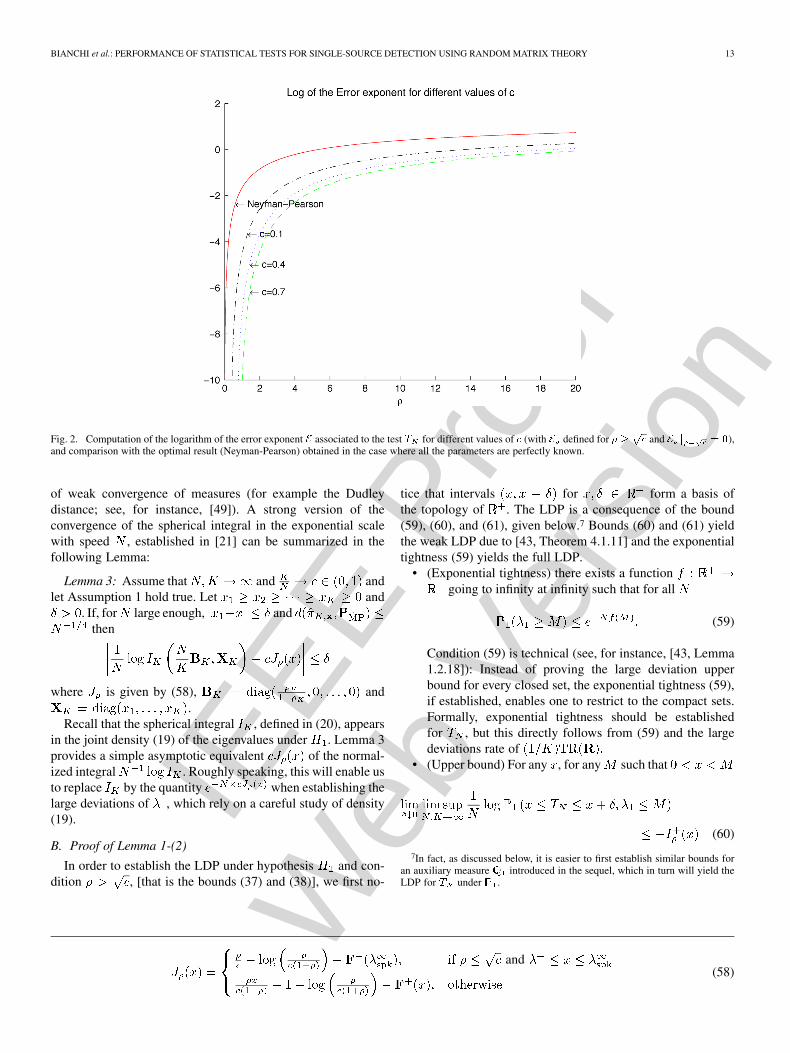
Fig. 2 compares the error exponent of test with the optimalNP test (assuming that all the parameters are known) for variousvalues of and . The error exponent of the NP test can be easilyobtained using Stein’s Lemma (see, for instance, [47]).
In Fig. 3, we compare the Error Exponent curves of both testsand . The analytic expressions provided in 2 and 3 for
the Error Exponent curves have been used to plot the curves.The asymptotic comparison clearly underlines the gain of usingtest .
Finally, we compare in Fig. 4 the powers (computed byMonte-Carlo methods) of tests and for finite valuesof and . We consider the case whereand and plot the probability of error under versusthe power of the test, that is versus (resp.
) where is fixed by the following condition:
VIII. CONCLUSION
In this contribution, we have analyzed in detail the GLRT inthe case where the noise variance and the channel are unknown.Unlike similar contributions, we have focused our efforts on theanalysis of the error exponent by means of large random matrixtheory and large deviation techniques. Closed-form expressionswere obtained and enabled us to establish that the GLRT asymp-totically outperforms the test based on the condition number,a fact that is supported by finite-dimension simulations. Wealso believe that the large deviations techniques introduced herewill be of interest for the engineering community, beyond theproblem addressed in this paper.
APPENDIX APROOF OF LEMMA 1: LARGE DEVIATIONS FOR
The large deviations of the largest eigenvalue of large randommatrices have already been investigated in various contexts,Gaussian Orthogonal Ensemble [48] and deformed Gaussianensembles [21]. As mentionned in [21, Remark 1.2], the proofsof the latter can be extended to complex Wishart matrix models,that is random matrices under or .
In both cases, the large deviations of rely on a close studyof the density of the eigenvalues, either given by (12) (under
) or by (19) for the spiked model (under ). The study ofthe spiked model, as it involves the study of the asymptotics ofthe spherical integral (see Lemma 3 below), is more difficult.We, therefore, focus on the proof of the LDP under (Lemma1-(2)) and omit the proof of Lemma 1-(1). Once Lemma 1-(2) isproved, proving Lemma 1-(1) is a matter of bookkeeping, withthe spherical integral removed at each step.
Recall that are the ordered eigenvalues ofand that is the statistics defined in (6).
In the sequel, we shall prove the upper bound of the LDPin Lemma 1-(2) [which gives also the upper bound in Lemma1-(3)]. The proof of the lower bound in Lemma 1-(3) requiresmore precise arguments than the lower bound of the LDP. Onehas indeed to study what happens at the vicinity of whichis a point of discontinuity of the rate function . Thus, we skipthe proof of the lower bound of the LDP in Lemma 1-(2) toavoid repetition. Note that the proof of Lemma 1-(4) is a mereconsequence of the fact that converges a.s. to if

IEEE
Pro
of
Web
Ver
sion
12 IEEE TRANSACTIONS ON INFORMATION THEORY, VOL. 57, NO. 4, APRIL 2011
Fig. 1. Plots of rate functions � and � in the case where � � ��� and � � � db. In this case, � � ������� � � �� � � � � and � � � �.
thus converges to 1 whenever converges to.
For the sake of simplicity and with no loss of generality asthe law of does not depend on we assume all along thisAppendix that . We first recall important asymptoticresults for spherical integrals.
A. Useful Facts About Spherical Integrals
Recall that the joint distributions of the ordered eigenvaluesunder hypothesis and are respectively given by (12) and
(19). In the latter, the so-called spherical integral (20) is intro-duced. We recall here results from [21] related to the asymptoticbehavior of the spherical integral in the case where one diagonalmatrix is of rank one and the other has the limiting distribution
. We first introduce the function defined for by(58), shown at the bottom of the next page.
Consider a -tuple and denote bythe empirical distribution associated to
; let be a metric compatible with the topology
IEEE
Pro
of
Web
Ver
sion
BIANCHI et al.: PERFORMANCE OF STATISTICAL TESTS FOR SINGLE-SOURCE DETECTION USING RANDOM MATRIX THEORY 13
Fig. 2. Computation of the logarithm of the error exponent � associated to the test � for different values of � (with � defined for � � �� and � � � �),
and comparison with the optimal result (Neyman-Pearson) obtained in the case where all the parameters are perfectly known.
of weak convergence of measures (for example the Dudleydistance; see, for instance, [49]). A strong version of theconvergence of the spherical integral in the exponential scalewith speed , established in [21] can be summarized in thefollowing Lemma:
Lemma 3: Assume that and andlet Assumption 1 hold true. Let and
. If, for large enough, andthen
where is given by (58), and.
Recall that the spherical integral , defined in (20), appearsin the joint density (19) of the eigenvalues under . Lemma 3provides a simple asymptotic equivalent of the normal-ized integral . Roughly speaking, this will enable usto replace by the quantity when establishing thelarge deviations of , which rely on a careful study of density(19).
B. Proof of Lemma 1-(2)
In order to establish the LDP under hypothesis and con-dition , [that is the bounds (37) and (38)], we first no-
tice that intervals for form a basis ofthe topology of . The LDP is a consequence of the bound(59), (60), and (61), given below.7 Bounds (60) and (61) yieldthe weak LDP due to [43, Theorem 4.1.11] and the exponentialtightness (59) yields the full LDP.
• (Exponential tightness) there exists a functiongoing to infinity at infinity such that for all
(59)
Condition (59) is technical (see, for instance, [43, Lemma1.2.18]): Instead of proving the large deviation upperbound for every closed set, the exponential tightness (59),if established, enables one to restrict to the compact sets.Formally, exponential tightness should be establishedfor , but this directly follows from (59) and the largedeviations rate of
• (Upper bound) For any , for any such that
(60)
7In fact, as discussed below, it is easier to first establish similar bounds foran auxiliary measure introduced in the sequel, which in turn will yield theLDP for � under .
and(58)

IEEE
Pro
of
Web
Ver
sion
14 IEEE TRANSACTIONS ON INFORMATION THEORY, VOL. 57, NO. 4, APRIL 2011
Fig. 3. Error Exponent curves associated to the tests � �� � and � �� � in the case where � � and � � �� dB. Each point of the curve corresponds to agiven error exponent under � (� axis) and its counterpart error exponent under � (� axis) as described in Theorem 2-(2) for � and Theorem 3-(2) for � .
Fig. 4. Simulated ROC curves for � (test 1) and � (test 2) in the case where � � �� � �� and � � �� dB.
Due to the exponential tightness, it is sufficient to establishthe upper bound for compact sets. As each compact can becovered by a finite number of balls, it is, therefore, suffi-cient to establish upper estimate (60) in order to establishthe LD upper bound.
• (Lower bound) For any
(61)
The fact that (61) implies the LD lower bound (38) is stan-dard in LD and can be found in [43, Chapter 1], for in-stance.
As the arguments are very similar to the ones developed in [21],we only prove in detail the upper bound (60). Proofs of (59) and(61) are left to the reader.
The idea is that the empirical measure
(of all but the largest eigenvalues) and thetrace concentrate faster than the largest eigenvalue. In theexponential scale with speed and the trace can be

IEEE
Pro
of
Web
Ver
sion
BIANCHI et al.: PERFORMANCE OF STATISTICAL TESTS FOR SINGLE-SOURCE DETECTION USING RANDOM MATRIX THEORY 15
considered as equal to their limit, respectively and 1. Inparticular, the deviations of arise from those of the largesteigenvalue and they both satisfy the same LDP with the samerate function . We, therefore, isolate the terms depending on
and gather the others through their empirical measure .Recall the notations introduced in (12) and (19) and let
. Consider the following domain:
for large enough
where we performed the change of variables for, and the related modifications and
. Note also that strictlyspeaking, the domain of integration would be expressed dif-ferently with the ’s and in particular, we should have changedconstant which majorizes the ’s into a larger constant as the
’s can theoretically be slightly above —we keep the samenotation for the sake of simplicity.
To proceed, one has to study the asymptotic behavior of thenormalizing constant
which turns out to be difficult. Instead of establishing directlythe bounds (59)–(61), we proceed as in [21] and establish similarbounds replacing the probability measures by the measures
defined as
and the rate function by the function defined by
for . Notice that these positive measures are notprobability measures any more, and as a consequence, the func-tion is not necessarily positive and its infimum might not beequal to zero, as it is the case for a rate function.
Writing the upper bound for , we obtain
where, for any compactly supported probability measure andany real number greater than the right edge of the support of
Let us now localize the empirical measure around 8
and the trace around 1. The continuity and convergence proper-ties of the spherical integral recalled in Lemma 3 yield, forlarge enough
(62)
with
and
Note that the bounds of the first integral in (62) follow from thefact that the event implies that
provided that is satisfied.The second term in (62) is easily obtained considering the factthat all the eigenvalues are less than so that for
and .Now, standard concentration results under yield that
8Notice that if �� is close to , so is �� due to the change of variable� � � .

IEEE
Pro
of
Web
Ver
sion
16 IEEE TRANSACTIONS ON INFORMATION THEORY, VOL. 57, NO. 4, APRIL 2011
More precisely, one knows using [50] that the empirical measureis close enough to its expectation and then using
[51] one knows that the expectation is close enough to its limit. The arguments are detailed in the Wigner case in [21] and
we do not give more details here.As for is continuous
and is lower semi-continuous, we obtain
By continuity in of the two involved functions, we finally get
and the counterpart of (60) is proved for and function .The proof of the lower bound is quite similar and left to thereader. It remains now to recover (60). As is a probabilitymeasure and the whole space is both open and closed, anapplication of the upper and lower bounds for immediatelyyields
(63)
This implies that the LDP holds for with rate function.
It remains to check that , which easilyfollows from the fact to be proved that
(64)
We, therefore, study the variations of over . Notethat , and thus that
. Function being a Stieltjes transform is in-creasing for , and so is , whose limit at infinityis . Straightforward but involved computations usingthe explicit representation (67) for yield that .Therefore, is decreasing on and increasing on
, and (64) is proved.This concludes the proof of the upper bound in Lemma 1-(2).
The proof of Lemma 1-(1) is very similar and left to the reader.
C. Proof of Lemma 1-(3)
The proof of this point requires an extra argument as we studythe large deviations of near the point where therate function is not continuous. In particular, the limit (53) doesnot follow from the LDP already established. As we shall seewhen considering , the factthat the scale is the same as the one of the fluctuationsof the largest eigenvalue of the complex Wishart model is cru-cial.
We detail the proof in the case when and, as above,consider the positive measures . We need to prove that
(65)
the other bound being a direct consequence of the LDP. As pre-viously, we will carefully localize the various quantities of in-terest. Denote by forand by for . Notice also that
together with imply that. We shall also consider the further constraints:
and
which enable us to properly separate from the support of. Now, with the localization indicated above, we have for
large enough
As previously, we consider the variables forand obtain, with the help of Lemma 3
with
IEEE
Pro
of
Web
Ver
sion
BIANCHI et al.: PERFORMANCE OF STATISTICAL TESTS FOR SINGLE-SOURCE DETECTION USING RANDOM MATRIX THEORY 17
Therefore
(recall that ). Now, as, its
contribution vanishes at the LD scale
It remains to check that is boundedbelow uniformly in . This will yield the convergence of
towards zero; hence, (65). Con-sider
We have already used the fact that the first term goes tozero when grows to infinity. Recall that the fluctuationsof are of order ; therefore, the second termalso goes to zero as we consider deviations of order .Now, converges in distribution tothe Tracy–Widom law; therefore, the last term converges to
. This concludes the proof.
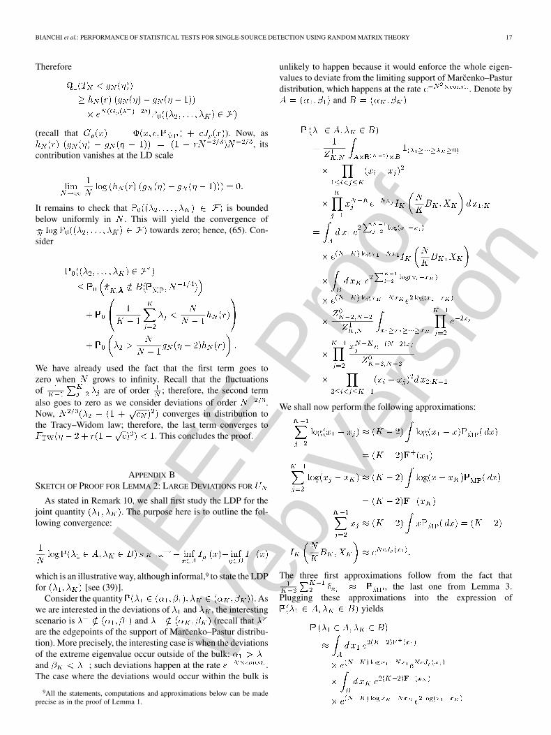
APPENDIX BSKETCH OF PROOF FOR LEMMA 2: LARGE DEVIATIONS FOR
As stated in Remark 10, we shall first study the LDP for thejoint quantity . The purpose here is to outline the fol-lowing convergence:
which is an illustrative way, although informal,9 to state the LDPfor [see (39)].
Consider the quantity . Aswe are interested in the deviations of and , the interestingscenario is and (recall thatare the edgepoints of the support of Marcenko–Pastur distribu-tion). More precisely, the interesting case is when the deviationsof the extreme eigenvalue occur outside of the bulk:and ; such deviations happen at the rate .The case where the deviations would occur within the bulk is
9All the statements, computations and approximations below can be madeprecise as in the proof of Lemma 1.
unlikely to happen because it would enforce the whole eigen-values to deviate from the limiting support of Marcenko–Pasturdistribution, which happens at the rate . Denote by
and
We shall now perform the following approximations:
The three first approximations follow from the fact that, the last one from Lemma 3.
Plugging these approximations into the expression ofyields

IEEE
Pro
of
Web
Ver
sion
18 IEEE TRANSACTIONS ON INFORMATION THEORY, VOL. 57, NO. 4, APRIL 2011
As and , the last integral goesto one as and
Recall that we are interested in the limit. The last term will account for a constant [see,
for instance, (63)]:
The term within the exponential in the integral ac-counts for the interraction between and and its contri-bution vanishes at the desired rate. In order to evaluate the tworemaining integrals, one has to rely on Laplace’s method (see,for instance, [52]) to express the leading term of the integrals(replacing by below)
Finally, we get the desired limit
where
It remains to replace by its expression (58) and to spreadthe constant over and , which are not a priori ratefunctions (recall that a rate function is nonnegative). If ,then the event is “typical” and no deviation occurs,otherwise stated, the rate function should satisfy
. Similarly, under and under
. Necessarily, should write under(resp. under ) and the rate functionsshould be given by:under (resp. under ), which are thedesired results.
We have proved (informally) that the LDP holds true forwith rate function . The contraction
principle [43, Chap. 4] immediatly yields the LDP for the ratiowith rate function
(66)
which is the desired result. We provide here intuitive argumentsto understand this fact.
For this, interpret the value of the rate function asthe cost associated to a deviation of (under ) around :
. If a deviation occurs forthe ratio , say where (which isthe typical behavior of under ), then necessarily mustdeviate around some value , so does around some value ,so that the ratio is around . In terms of rate functions, the costof the joint deviation is .The true cost associated to the deviation of the ratio will be theminimum cost among all these possible joint deviations ofand ; hence, the rate function (66).
APPENDIX CCLOSED-FORM EXPRESSIONS FOR FUNCTIONS AND
Consider the Stieltjes transform of Marcenko–Pastur distri-bution
We gather without proofs a few facts related to , which are partof the folklore.
Lemma 4 (Representation of ): The following hold true:1) Function is analytic in .2) If with , then
where stands for the principal branch of the square-root.
3) If with , then
where stands for the branch of the square-root whoseimage is .
4) As a consequence, the following hold true:
(67)
(68)

IEEE
Pro
of
Web
Ver
sion
BIANCHI et al.: PERFORMANCE OF STATISTICAL TESTS FOR SINGLE-SOURCE DETECTION USING RANDOM MATRIX THEORY 19
5) Consider the following function . Func-tions and satisfy the following system of equations:
(69)
Recall the definition (31) and (51) of function and .In the following lemma, we provide closed-form formulas ofinterest.
Lemma 5: The following identities hold true:1) Let then
2) Let then
Proof: Consider the case where . First write
Integrating with respect with and applying Funini’s the-orem yields
in the case where . Recall that and are holomorphicfunctions over and satisfy system (69)(notice in particular that and never vanish). Usingthe first equation of (69) implies that
(70)
Consider . By adirect computation of the derivative, we get
Hence
It remains to plug this identity into (70) to conclude. The repre-sentation of can be established similarly.
ACKNOWLEDGMENT
The authors would like to thank O. Cappé for many fruitfuldiscussions related to the GLRT.
REFERENCES
[1] J. Mitola, III and G. Q. Maguire, Jr., “Cognitive radio: Making soft-ware radios more personal,” IEEE Wireless Commun., vol. 6, pp. 13–18,1999.
[2] S. Haykin, “Cognitive radio: Brain-empowered wireless communica-tions,” IEEE J. Sel. Areas Commun., vol. 23, no. 2, pp. 201–220, Feb.2005.
[3] M. Dohler, E. Lefranc, and A. H. Aghvami, “Virtual antenna arraysfor future wireless mobile communication systems,” ICT. Beijing,China, 2002.
[4] H. Urkowitz, Energy Detection of Unknown Deterministic Signals, vol.55, no. 4, pp. 523–531, Apr. 1967.
[5] V. I. Kostylev, “Energy detection of a signal with random amplitude,”in Proc. IEEE Int. Conf. Communications, 2002, vol. 3, pp. 1606–1610.
[6] F. F. Digham, M.-S. Alouini, and M. K. Simon, “On the energy de-tection of unknown signals over fading channels,” in Proc. IEEE Int.Conf. Communications, May 2003, vol. 5, pp. 3575–3579.
[7] Z. Quan, S. Cui, A. H. Sayed, and H. V. Poor, “Spatial-spectral jointdetection for wideband spectrum sensing in cognitive radio networks,”presented at the ICASSP, Las Vegas, 2008.
[8] E. L. Lehman and J. P. Romano, Testing Statistical Hypotheses. NewYork: Springer, 2006, Springer Texts in Statistics.
[9] M. Wax and T. Kailath, “Detection of signals by information theoreticcriteria,” IEEE Trans. Signal, Speech, Signal Process., vol. 33, no. 2,pp. 387–392, Apr. 1985.
[10] P.-J. Chung, J. F. Bohme, C. F. Mecklenbrauker, and A. O. Hero, “De-tection of the number of signals using the Benjamini–Hochberg proce-dure,” IEEE Trans. Signal Process., vol. 55, no. 6, pp. 2497–2508, Jun.2007.
[11] A. Taherpour, M. Nasiri-Kenari, and S. Gazor, “Multiple antenna spec-trum sensing in cognitive radios,” IEEE Trans. Wireless Commun., vol.9, no. 2, pp. 814–823, 2010.
[12] X. Mestre, “Improved estimation of eigenvalues and eigenvectors ofcovariance matrices using their sample estimates,” IEEE Trans. Inf.Theory, vol. 54, no. 11, pp. 5113–5129, Nov. 2008.
[13] X. Mestre, “On the asymptotic behavior of the sample estimates ofeigenvalues and eigenvectors of covariance matrices,” IEEE Trans.Signal Process., vol. 56, no. 11, pp. 5353–5368, Nov. 2008.
[14] S. Kritchman and B. Nadler, “Determining the number of componentsin a factor model from limited noisy data,” Chemometrics and Intelli-gent Laboratory Systems, 2008, 1932, 94.
[15] S. Kritchman and B. Nadler, “Non-parametric detection of the numberof signals: Hypothesis testing and random matrix theory,” IEEE Trans.Signal Process., vol. 57, no. 10, pp. 3930–3941, Oct. 2009.
[16] J. Silverstein and P. Combettes, “Signal detection via spectral theoryof large dimensional random matrices,” IEEE Trans. Signal Process.,vol. 40, no. 8, pp. 2100–2105, Aug. 1992.
[17] R. Couillet and M. Debbah, “A Bayesian framework for collabo-rative multi-source signal detection,” IEEE Trans. Signal Process.,arxiv:0811.0764, to be published.
[18] N. R. Rao, J. A. Mingo, R. Speicher, and A. Edelman, “Statisticaleigen-inference from large Wishart matrices,” Ann. Statist., vol. 36, no.6, pp. 2850–2885, 2008.
[19] R. R. Nadakuditi and J. W. Silverstein, “Fundamental limit of samplegeneralized eigenvalue based detection of signals in noise using rela-tively few signal-bearing and noise-only samples,” IEEE J. Sel. TopicsSignal Process., vol. 4, no. 3, pp. 468–480, Jun. 2010.
[20] I. M. Johnstone, “On the distribution of the largest eigenvalue in prin-cipal components analysis,” Ann. Statist., vol. 29, no. 2, pp. 295–327,2001.
[21] M. Maida, “Large deviations for the largest eigenvalue of rank one de-formations of Gaussian ensembles,” Electron. J. Probab., vol. 12, pp.1131–1150, 2007, (electronic).
[22] Y. H. Zeng and Y. C. Liang, Eigenvalue Based Spectrum Sensing Al-gorithms for Cognitive Radio, Tech. Rep., 2008, arXiv:0804.2960v1.
[23] L. S. Cardoso, M. Debbah, P. Bianchi, and J. Najim, “Cooperative spec-trum sensing using random matrix theory,” in Proc. 3rd Int. Symp. Wire-less Pervasive Computing, May 2008, pp. 334–338.
[24] F. Penna, R. Garello, and M. Spirito, “Cooperative spectrum sensingbased on the limiting eigenvalue ratio distribution in Wishart matrices,”IEEE Commun. Lett., vol. 13, no. 7, pp. 507–509, Jul. 2009.

IEEE
Pro
of
Web
Ver
sion
20 IEEE TRANSACTIONS ON INFORMATION THEORY, VOL. 57, NO. 4, APRIL 2011
[25] T. Abbas, N.-K. Masoumeh, and G. Saeed, “Multiple antenna spec-trum sensing in cognitive radios,” IEEE Trans. Wireless Commun., tobe published.
[26] T. W. Anderson, “Asymptotic theory for principal component anal-ysis,” J. Math. Statist., vol. 34, pp. 122–148, 1963.
[27] A. W. van der Vaart, “Asymptotic statistics,” in Cambridge Series inStatistical and Probabilistic Mathematics. Cambridge, U.K.: Cam-bridge Univ. Press, 1998, vol. 3.
[28] M. L. Mehta, Random Matrices Volume 142 of Pure and Applied Math-ematics (Amsterdam), 3rd ed. Amsterdam, The Netherlands: Else-vier/Academic Press, 2004.
[29] G. Anderson, A. Guionnet, and O. Zeitouni, An Introduction toRandom Matrices. Cambridge, U.K.: Cambridge Univ. Press, 2009,Cambridge Studies in Advanced Mathematics.
[30] R. J. Muirhead, Aspects of Multivariate Statistical Theory, ser. WileySeries in Probability and Mathematical Statistics. Hoboken, NJ:Wiley, 1982.
[31] P. Koev, Random Matrix Statistics Toolbox [Online]. Available: http://math.mit.edu/plamen/software/rmsref.html
[32] P. Koev and A. Edelman, “The efficient evaluation of the hypergeo-metric function of a matrix argument,” Math. Comp., vol. 75, no. 254,pp. 833–846, 2006, (electronic).
[33] J. Mitola, “Cognitive Radio An Integrated Agent Architecture for Soft-ware Defined Radio,” Ph.D. dissertation, Royal Inst. Technol. (KTH),Stockholm, Sweden, May 2000.
[34] V. A. Marcenko and L. A. Pastur, “Distribution of eigenvalues in cer-tain sets of random matrices,” Mat. Sb. (N.S.), vol. 72, no. 114, pp.507–536, 1967.
[35] G. Ben Arous and A. Guionnet, “Large deviations for Wigner’s lawand Voiculescu’s non-commutative entropy,” Probab. Theory RelatedFields, vol. 108, no. 4, pp. 517–542, 1997.
[36] B. Nadler, “On the distribution of the ratio of the largest eigenvalue tothe trace of a wishart matrix,” Ann. Statist. [Online]. Available: http://www.wisdom.weizmann.ac.il/~nadler/ 2010
[37] C. A. Tracy and H. Widom, “Level-spacing distributions and the Airykernel,” Comm. Math. Phys., vol. 159, no. 1, pp. 151–174, 1994.
[38] C. A. Tracy and H. Widom, “On orthogonal and symplectic matrixensembles,” Comm. Math. Phys., vol. 177, no. 3, pp. 727–754, 1996.
[39] A. Bejan, “Largest eigenvalues and sample covariance matrices,”Tracy–Widom and Painleve II: Computational Aspects and Re-alization in S-Plus With Applications 2005 [Online]. Available:http://www.vitrum.md/andrew/TWinSplus.pdf
[40] F. Bornemann, “Asymptotic independence of the extreme eigenvaluesof Gaussian unitary ensemble,” J. Math. Phys., vol. 51, no. 2, p. 023514,8, 2010.
[41] J. Baik and J. Silverstein, “Eigenvalues of large sample covariance ma-trices of spiked population models,” J. Multivariate Anal., vol. 97, no.6, pp. 1382–1408, 2006.
[42] P. J. Bickel and P. W. Millar, “Uniform convergence of probabilitymeasures on classes of functions,” Statist. Sinica, vol. 2, no. 1, pp. 1–15,1992.
[43] A. Dembo and O. Zeitouni, Large Deviations Techniques and Applica-tions, 2nd ed. New York: Springer Verlag, 1998.
[44] Y. Q. Yin, Z. D. Bai, and P. R. Krishnaiah, “On the limit of thelargest eigenvalue of the large-dimensional sample covariance matrix,”Probab. Theory Related Fields, vol. 78, no. 4, pp. 509–521, 1988.
[45] Z. D. Bai and Y. Q. Yin, “Limit of the smallest eigenvalue of a large-dimensional sample covariance matrix,” Ann. Probab., vol. 21, no. 3,pp. 1275–1294, 1993.
[46] P. Bianchi, M. Debbah, and J. Najim, “Asymptotic independence inthe spectrum of the Gaussian unitary ensemble,” Electron. Commun.Probab. vol. 15, Sep. 2010, pp. 376–395.
[47] P.-N. Chen, “General formulas for the Neyman-Pearson type-II errorexponent subject to fixed and exponential type-i error bounds,” IEEETrans. Inf. Theory, vol. 42, no. 1, pp. 316–323, Jan. 1996.
[48] G. Ben Arous, A. Dembo, and A. Guionnet, “Aging of spherical spinglasses,” Probab. Theory Related Fields, vol. 120, no. 1, pp. 1–67,2001.
[49] R. M. Dudley, Real Analysis and Probability, Volume 74 of CambridgeStudies in Advanced Mathematics. Cambridge, U.K.: CambridgeUniv. Press, 2002, revised reprint of the 1989 original.
[50] A. Guionnet and O. Zeitouni, “Concentration of the spectral measurefor large matrices.,” Electron. Comm. Probab., vol. 5, pp. 119–136,2000, (electronic).
[51] Z. D. Bai, “Convergence rate of expected spectral distributions of largerandom matrices. II. Sample covariance matrices,” Ann. Probab., vol.21, no. 2, pp. 649–672, 1993.
[52] J. Dieudonné, Infinitesimal Calculus. Paris, France: Hermann, 1971,translated from French.
P. Bianchi was born in 1977 in Nancy, France. He received the M.Sc. degreefrom Supélec-Paris XI, France, in 2000, and the Ph.D. degree from the Univer-sity of Marne-la-Vallée, France, in 2003.
From 2003 to 2009, he was an Associate Professor with the Telecommuni-cation Department of Supélec. In 2009, he joined the Statistics and Applica-tions Group at LTCI-Telecom ParisTech. His current research interests are in thearea of statistical signal processing for sensor networks. They include decentral-ized detection, quantization, adaptive algorithms for distributed estimation, andrandom matrix theory.
M. Debbah was born in Madrid, Spain. He entered the Ecole NormaleSupérieure de Cachan, France, in 1996 where he received the M.Sc. and Ph.D.degrees in 1999 and 2002, respectively.
From 1999 to 2002, he was with Motorola Labs, working on wireless localarea networks and prospective fourth generation systems. From 2002 until 2003,he was appointed Senior Researcher at the Vienna Research Center for Telecom-munications (FTW) (Vienna, Austria). From 2003 until 2007, he was with theMobile Communications department of the Institut Eurecom (Sophia Antipolis,France) as an Assistant Professor. He is presently a Professor at Supélec (Gif-sur-Yvette, France), holder of the Alcatel-Lucent Chair on Flexible Radio. Hisresearch interests are in information theory, signal processing, and wireless com-munications.
Prof. Debbah is the recipient of the “Mario Boella” prize award in 2005, the2007 General Symposium IEEE GLOBECOM best paper award, the Wi-Opt2009 best paper award, the 2010 Newcom�� best paper award, as well asthe Valuetools 2007, Valuetools 2008, and CrownCom2009 best student paperawards. He is a WWRF fellow.
M. Maida received the Ph.D. degree from the Ecole normale supérieure, Lyon,France, in 2004.
She is a former student of the Ecole normale supérieure, Paris, France. Since2005, she has been an Associate Professor at the University Paris-Sud, Orsay.Her research interests include random matrices theory, large deviations, and freeprobability.
J. Najim received his engineering diploma from Télécom Paristech, France, in1998, and the Ph.D. degree from University Nanterre Paris-10 in 2001.
Since 2002, he has been with the Centre National de la Recherche Scien-tifique (CNRS) and Télécom Paristech. His research interests include wirelesscommunication, the theory of random matrices, and probability at large.

IEEE
Pro
of
Prin
t Ver
sion
IEEE TRANSACTIONS ON INFORMATION THEORY, VOL. 57, NO. 4, APRIL 2011 1
Performance of Statistical Tests for Single-SourceDetection Using Random Matrix Theory
P. Bianchi, M. Debbah, M. Maida, and J. Najim
Abstract—This paper introduces a unified framework for the de-tection of a single source with a sensor array in the context wherethe noise variance and the channel between the source and the sen-sors are unknown at the receiver. The Generalized Maximum Like-lihood Test is studied and yields the analysis of the ratio betweenthe maximum eigenvalue of the sampled covariance matrix and itsnormalized trace. Using recent results from random matrix theory,a practical way to evaluate the threshold and the �-value of the testis provided in the asymptotic regime where the number � of sen-sors and the number � of observations per sensor are large buthave the same order of magnitude. The theoretical performance ofthe test is then analyzed in terms of Receiver Operating Character-istic (ROC) curve. It is, in particular, proved that both Type I andType II error probabilities converge to zero exponentially as thedimensions increase at the same rate, and closed-form expressionsare provided for the error exponents. These theoretical results relyon a precise description of the large deviations of the largest eigen-value of spiked random matrix models, and establish that the pre-sented test asymptotically outperforms the popular test based onthe condition number of the sampled covariance matrix.
Index Terms—Cooperative spectrum sensing, generalized likeli-hood ratio test, hypothesis testing, large deviations, random matrixtheory, ROC curve.
I. INTRODUCTION
T HE detection of a source by a sensor array is at the heartof many wireless applications. It is of particular interest in
the realm of cognitive radio [1], [2] where a multisensor cogni-tive device (or a collaborative network1) needs to discover orsense by itself the surrounding environment. This allows thecognitive device to make relevant choices in terms of informa-tion to feed back, bandwidth to occupy or transmission power touse. When the cognitive device is switched on, its prior knowl-edge (on the noise variance for example) is very limited and canrarely be estimated prior to the reception of data. This unfortu-nately rules out classical techniques based on energy detection[4]–[6] and requires new sophisticated techniques exploiting thespace or spectrum dimension.
Manuscript received October 02, 2009; revised April 01, 2010; acceptedAugust 10, 2010. This work was supported in part by the French programsANR-07-MDCO-012-01 “Sesame” and ANR-08-BLAN-0311-03 “GranMa”.
P. Bianchi and J. Najim are with CNRS/Télécom Paristech, France (e-mail:[email protected]; [email protected]).
M. Debbah is with Supélec, Gif-sur-Yvette, France (e-mail: [email protected]).
M. Maida is with the Université Paris-Sud, UMR CNRS 8628, France (e-mail:[email protected]).
Communicated by A. L. Moustakas, Associate Editor for Communications.Digital Object Identifier 10.1109/TIT.2011.2111710
1The collaborative network corresponds to multiple base stations connected,in a wireless or wired manner, to form a virtual antenna system [3].
In our setting, the aim of the multisensor cognitive detectionphase is to construct and analyze tests associated with the fol-lowing hypothesis testing problem:
(1)
where is the observed com-plex time series, represents a complex circularGaussian white noise process with unknown variance , andrepresents the number of received samples. Vector isa deterministic vector and typically represents the propagationchannel between the source and the sensors. Signal de-notes a standard scalar independent and identically distributed(i.i.d.) circular complex Gaussian process with respect to thesamples and stands for the source signal to bedetected.
The standard case where the propagation channel and thenoise variance are known has been thoroughly studied in theliterature in the Single Input Single Output case [4]–[6] andMulti-Input Multi-Ouput [7] case. In this simple context, themost natural approach to detect the presence of source isthe well-known Neyman-Pearson (NP) procedure which con-sists in rejecting the null hypothesis when the observed like-lihood ratio lies above a certain threshold [8]. Traditionally,the value of the threshold is set in such a way that the Prob-ability of False Alarm (PFA) is no larger than a predefined level
. Recall that the PFA (resp. the miss probability) ofa test is defined as the probability that the receiver decides hy-pothesis (resp. ) when the true hypothesis is (resp.
). The NP test is known to be uniformly most powerful i.e.,for any level , the NP test has the minimum achiev-able miss probability (or equivalently the maximum achievablepower) among all tests of level . In this paper, we assume that:
• the noise variance is unknown;• vector is unknown.
In this context, probability density functions of the observationsunder both and are unknown, and the classical NP
approach can no longer be employed. As a consequence, theconstruction of relevant tests for (1) together with the analysisfo their perfomances is a crucial issue. The classical approachfollowed in this paper consists in replacing the unknown pa-rameters by their maximum likelihood estimates. This leads tothe so-called Generalized Likelihood Ratio (GLR). The Gener-alized Likelihood Ratio Test (GLRT), which rejects the null hy-pothesis for large values of the GLR, easily reduces to the sta-tistics given by the ratio of the largest eigenvalue of the sampledcovariance matrix to its normalized trace, cf. [9]–[11]. Nearby
0018-9448/$26.00 © 2011 IEEE

IEEE
Pro
of
Prin
t Ver
sion
2 IEEE TRANSACTIONS ON INFORMATION THEORY, VOL. 57, NO. 4, APRIL 2011
statistics [12]–[15], with good practical properties, have alsobeen developed, but do not yield a different (asymptotic) errorexponent analysis.
In this paper, we analyze the performance of the GLRT inthe asymptotic regime where the number of sensors and thenumber of observations per sensor are large but have the sameorder of magnitude. This assumption is relevant in many appli-cations, among which cognitive radio, for instance, and casts theproblem into a large random matrix framework.
Large random matrix theory has already been applied tosignal detection [16] (see also [17]), and recently to hypothesistesting [15], [18], [19]. In this article, the focus is mainlydevoted to the study of the largest eigenvalue of the sampledcovariance matrix, whose behavior changes under or .The fluctuations of the largest eigenvalue under havebeen described by Johnstone [20] by means of the celebratedTracy–Widom distribution, and are used to study the thresholdand the -value of the GLRT.
In order to characterize the performance of the test, a naturalapproach would be to evaluate the Receiver Operating Charac-teristic (ROC) curve of the GLRT, that is to plot the power of thetest versus a given level of confidence. Unfortunately, the ROCcurve does not admit any simple closed-form expression for afinite number of sensors and snapshots. As the miss probabilityof the GLRT goes exponentially fast to zero, the performance ofthe GLRT is analyzed via the computation of its error exponent,which characterizes the speed of decrease to zero. Its compu-tation relies on the study of the large deviations of the largesteigenvalue of “spiked” sampled covariance matrix. By “spiked”we refer to the case where the eigenvalue converges outside thebulk of the limiting spectral distribution, which precisely hap-pens under hypothesis . We build upon [21] to establish thelarge deviation principle, and provide a closed-form expressionfor the rate function.
We also introduce the error exponent curve, and plot the errorexponent of the power of the test versus the error exponent for agiven level of confidence. The error exponent curve can be inter-preted as an asymptotic version of the ROC curve in ascale and enables us to establish that the GLRT outperformsanother test based on the condition number, and proposed by[22]–[24] in the context of cognitive radio.
Notice that the results provided here (determination of thethreshold of the GLRT test and the computation of the errorexponents) would still hold within the setting of real Gaussianrandom variables instead of complex ones, with minor modifi-cations.2
The paper is organized as follows.Section II introduces the GLRT. The value of the threshold,
which completes the definition of the GLRT, is established inSection II-B. As the latter threshold has no simple closed-formexpression and as its practical evaluation is difficult, we intro-duce in Section II-C an asymptotic framework where it is as-sumed that both the number of sensors and the number ofavailable snapshots go to infinity at the same rate. This assump-tion is valid, for instance, in cognitive radio contexts and yields
2Details are provided in Remarks 4 and 9.
a very simple evaluation of the threshold, which is important inreal-time applications.
In Section III, we recall several results of large random matrixtheory, among which the asymptotic fluctuations of the largesteigenvalue of a sample covariance matrix, and the limit of thelargest eigenvalue of a spiked model.
These results are used in Section IV where an approximatethreshold value is derived, which leads to the same PFA as theoptimal one in the asymptotic regime. This analysis yields a rel-evant practical method to approximate the -values associatedwith the GLRT.
Section V is devoted to the performance analysis of theGLRT. We compute the error exponent of the GLRT, derive itsexpression in closed-form by establishing a Large DeviationPrinciple for the test statistic ,3 and describe the errorexponent curve.
Section VI introduces the test based on the condition number,that is the statistics given by the ratio between the largest eigen-value and the smallest eigenvalue of the sampled covariance ma-trix. We provide the error exponent curve associated with thistest and prove that the latter is outperformed by the GLRT.
Section VII provides further numerical illustrations and con-clusions are drawn in Section VIII.
Mathematical details are provided in the Appendix. In partic-ular, a full rigorous proof of a large deviation principle is pro-vided in Appendix A, while a more informal proof of a nearbylarge deviation principle, maybe more accessible to the nonspe-cialist, is provided in Appendix B.
Notations: For represents the probabilityof a given event under hypothesis . For any real randomvariable and any real number , notation
stands for the test function which rejects the null hypothesiswhen . In this case, the probability of false alarm (PFA)of the test is given by , while the power of the testis . Notation stands for the almost sure (a.s.)convergence under hypothesis . For any one-to-one mapping
where and are two sets, we denote bythe inverse of w.r.t. composition. For any borel set
denotes the indicator function of set and de-notes the Euclidian norm of a given vector . If is a given ma-trix, denote by its transpose-conjugate. If is a cumulativedistribution function (c.d.f.), we denote by is complementaryc.d.f., that is: .
II. GENERALIZED LIKELIHOOD RATIO TEST
In this section, we derive the Generalized Likelihood RatioTest (Section II-A) and compute the associated threshold and
-value (Section II-B). This exact computation raises some
3Note that in recent papers [25], [14], [15], the fluctuations of the test statisticsunder� , based on large random matrix techniques, have also been used to ap-proximate the power of the test. We believe that the performance analysis basedon the error exponent approach, although more involved, has a wider range ofvalidity.
IEEE
Pro
of
Prin
t Ver
sion
BIANCHI et al.: PERFORMANCE OF STATISTICAL TESTS FOR SINGLE-SOURCE DETECTION USING RANDOM MATRIX THEORY 3
computational issues, which are circumvented by the intro-duction of a relevant asymptotic framework, well-suited formathematical analysis (Section II-C).
A. Derivation of the Test
Denote by the number of observed samples and recall that
where represents an independentand identically distributed (i.i.d.) process of vectors withcircular complex Gaussian entries with mean zero and covari-ance matrix , vector is deterministic, signal
denotes a scalar i.i.d. circular complexGaussian process with zero mean and unit variance. Moreover,
and are as-sumed to be independent processes. We stack the observed datainto a matrix . Denote bythe sampled covariance matrix
and respectively, by and the likelihoodfunctions of the observation matrix indexed by the unknownparameters and under hypotheses and .
As is a matrix whose columns are i.i.d. Gaussianvectors with covariance matrix defined by
(2)
likelihood functions write
(3)
(4)
In the case where parameters and are available, thecelebrated Neyman-Pearson procedure yields a uniformly most
powerful test, given by the likelihood ratio statistics .However, in the case where and are unknown, which
is the problem addressed here, no simple procedure garantees auniformly most powerful test, and a classical approach consistsin computing the GLR
(5)
In the GLRT procedure, one rejects hypothesis whenever, where is a certain threshold which is selected in
order that the PFA does not exceed a given level.In the following proposition, which follows after straightfor-
ward computations from [26] and [9], we derive the closed formexpression of the GLR . Denote by
the ordered eigenvalues of (all distincts with probabilityone).
Proposition 1: Let be defined by
(6)
then, the GLR [cf. (5)] writes
where .By Proposition 1, where
. The GLRT rejects the null hypothesiswhen inequality holds. As with prob-ability one and as is increasing on this interval, the latterinequality is equivalent to . Otherwise stated,the GLRT reduces to the test which rejects the null hypothesisfor large values of
(7)
where is a certain threshold which is such thatthe PFA does not exceed a given level . In the sequel, we will,therefore, focus on the test statistics .
Remark 1: There exist several variants of the above statis-tics [12]–[15], which merely consist in replacing the normalizedtrace with a more involved estimate of the noise variance. Al-though very important from a practical point of view, these vari-ants have no impact on the (asymptotic) error exponent analysis.Therefore, we restrict our analysis to the traditional GLRT forthe sake of simplicity.
B. Exact Threshold and -Values
In order to complete the construction of the test, we must pro-vide a procedure to set the threshold . As usual, we proposeto define as the value which maximizes the power
of the test (7) while keeping the PFA undera desired level . It is well-known (see, for instance,[8] and [27]) that the latter threshold is obtained by
(8)
where represents the complementary c.d.f. of the statis-tics under the null hypothesis
(9)
Note that is continuous and decreasing from 1 to 0 on, so that the threshold in (8) is always well
defined. When the threshold is fixed to , the GLRTrejects the null hypothesis when or equivalently,when . It is usually convenient to rewrite the GLRTunder the following form:
(10)

IEEE
Pro
of
Prin
t Ver
sion
4 IEEE TRANSACTIONS ON INFORMATION THEORY, VOL. 57, NO. 4, APRIL 2011
The statistics represents the significance probability or-value of the test. The null hypothesis is rejected when the-value is below the level . In practice, the compu-
tation of the -value associated with one experiment is of primeimportance. Indeed, the -value not only allows to accept/rejecta hypothesis by (10), but it furthermore reflects how strongly thedata contradicts the null hypothesis [8].
In order to evaluate -values, we derive in the sequel the exactexpression of the complementary c.d.f. . The crucial pointis that is a function of the eigenvalues of thesampled covariance matrix . We have
(11)
where for each , the domain of integration is defined by
and is the joint probability density function (p.d.f.) of theordered eigenvalues of under given by
(12)
where stands for the indicator function of theset and where is thenormalization constant (see, for instance, [28], [29, Chapter 4]).
Remark 2: For each , the computation of requires anumerical evaluation of a nontrivial integral. Despite the factthat powerful numerical methods, based on representations ofsuch integrals with hypergeometric functions [30], are available(see, for instance, [31] and [32]), an on line computation, re-quested in a number of real-time applications, may be out ofreach.
Instead, tables of the function should be computed off linei.e., prior to the experiment. As both the dimensions andmay be subject to frequent changes,4 all possible tables of thefunction should be available at the detector’s side, for allpossible values of the couple . This requires both sub-stantial computations and considerable memory space. In whatfollows, we propose a way to overcome this issue.
In the sequel, we study the asymptotic behavior of the com-plementary c.d.f. when both the number of sensors andthe number of snapshots go to infinity at the same rate. Thisanalysis leads to simpler testing procedure.
C. Asymptotic Framework
We propose to analyze the asymptotic behavior of the com-plementary c.d.f. as the number of observations goes toinfinity. More precisely, we consider the case where both the
4In cognitive radio applications, for instance, the number of users � whichare connected to the network is frequently varying.
number of sensors and the number of snapshots go to in-finity at the same speed, as assumed below
with(13)
This asymptotic regime is relevant in cases where the sensingsystem must be able to perform source detection in a moderateamount of time i.e., the number of sensors and the numberof samples being of the same order. This is in particular the casein cognitive radio applications (see, for instance, [33]). Veryoften, the number of sensors is lower than the number of snap-shots; hence, the ratio is lower than 1.
In the sequel, we will simply denote to refer tothe asymptotic regime (13).
Remark 3: The results related to the GLRT presented inSections IV and V remain true for ; in the case of the testbased on the condition number and presented in Section VI,extra-work is needed to handle the fact that the lowest eigen-value converges to zero, which happens if .
III. LARGE RANDOM MATRICES—LARGEST
EIGENVALUE—BEHAVIOR OF THE GLR STATISTICS
In this section, we recall a few facts on large random matricesas the dimensions go to infinity. We focus on the behaviorof the eigenvalues of which differs whether hypothesisholds (Section III-A) or holds (Section III-B).
As the column vectors of are i.i.d. complex Gaussian withcovariance matrix given by (2), the probability density ofis given by
where is a normalizing constant.
A. Behavior Under Hypothesis
As the behavior of does not depend on , we assume that; in particular, . Under , matrix is a com-
plex Wishart matrix and it is well-known (see, for instance, [28])that the Jacobian of the transformation between the entries of thematrix and the eigenvalues/angles is given by the Vandermondedeterminant . This yields the joint p.d.f.of the ordered eigenvalues (12) where the normalizing constant
is denoted by for simplicity.The celebrated result from Marcenko and Pastur [34] states
that the limit as of the c.d.f.associated to the empirical distribution of the eigenvaluesof is equal to where represents theMarcenko–Pastur distribution
(14)
with and . This convergence isvery fast in the sense that the probability of deviating fromdecreases as . More precisely, a simple application
IEEE
Pro
of
Prin
t Ver
sion
BIANCHI et al.: PERFORMANCE OF STATISTICAL TESTS FOR SINGLE-SOURCE DETECTION USING RANDOM MATRIX THEORY 5
of the large deviations results in [35] yields that for any distanceon the set of probability measures on compatible with the
weak convergence and for any
(15)
Moreover, the largest eigenvalue of converges a.s. tothe right edge of the Marcenko–Pastur distribution, that is
. A further result due to Johnstone [20] describes its speedof convergence and its fluctuations (see also [36] forcomplementary results). Let be defined by
(16)
where is defined by
(17)
then converges in distribution toward a standardTracy–Widom random variable with c.d.f. definedby
(18)
where solves the Painlevé II differential equation
and where Ai denotes the Airy function. In particular,is continuous. The Tracy–Widom distribution was first intro-duced in [37], [38] as the asymptotic distribution of the centeredand rescaled largest eigenvalue of a matrix from the GaussianUnitary Ensemble.
Tables of the Tracy–Widom law are available, for instance, in[39], while a practical algorithm allowing to efficiently evaluate(18) can be found in [40].
Remark 4: In the case where the entries of matrix are realGaussian random variables, the fluctuations of the largest eigen-value are still described by a Tracy–Widom distribution whosedefinition slightly differs from the one given in the complex case(for details, see [20]).
B. Behavior Under Hypothesis
In this case, the covariance matrix writesand matrix follows a single spiked model. Since the behaviorof is not affected if the entries of are multiplied by a givenconstant, we find it convenient to consider the model where
. Denote by
the signal-to-noise ratio (SNR), then matrix admits the de-composition where is a unitary matrix and
. With the same change of variablesfrom the entries of the matrix to the eigenvalues/angles with Ja-cobian the p.d.f. of the ordered eigen-values writes
(19)
where the normalizing constant is denotedby for simplicity, is the diagonal matrix with eigen-values is the diagonal matrix witheigenvalues , and for any real diagonal ma-trices the spherical integral is definedas
(20)
with the Haar measure on the unitary group of size (see[30Chapter 3] for details).
Whereas this rank-one perturbation does not affect theasymptotic behavior of (the convergence toward andthe deviations of the empirical measure given by (15) still holdunder ), the limiting behavior of the largest eigenvaluecan change if the signal-to-noise ratio is large enough.
Assumption 1: The following constant exists
(21)
We refer to as the limiting SNR. We also introduce
Under hypothesis , the largest eigenvalue has the followingasymptotic behavior as go to infinity
(22)
see, for instance, [41] for a proof of this result. Note in particularthat is strictly larger than the right edge of the supportwhenever . Otherwise stated, if the perturbation is largeenough, the largest eigenvalue converges outside the support ofMarcenko–Pastur distribution.
C. Limiting Behavior of Under and
Gathering the results recalled in Sections III-A and III-B, weobtain the following:
Proposition 2: Let Assumption 1 hold true and assume that, then
and
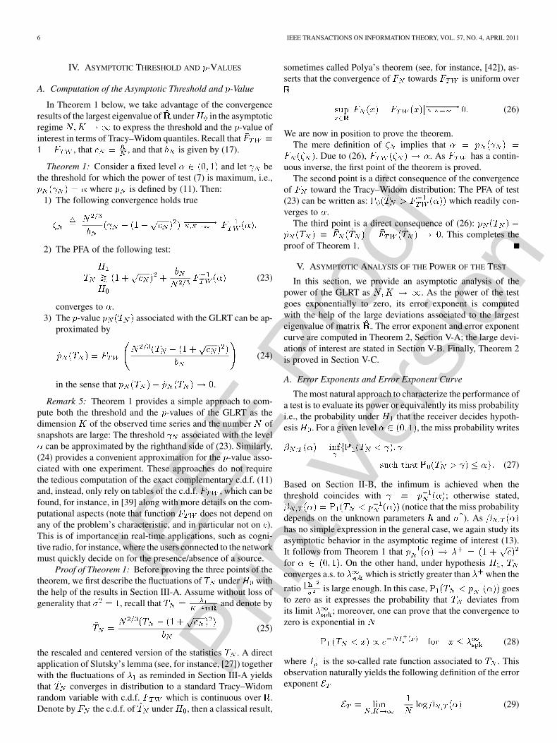
IEEE
Pro
of
Prin
t Ver
sion
6 IEEE TRANSACTIONS ON INFORMATION THEORY, VOL. 57, NO. 4, APRIL 2011
IV. ASYMPTOTIC THRESHOLD AND -VALUES
A. Computation of the Asymptotic Threshold and -Value
In Theorem 1 below, we take advantage of the convergenceresults of the largest eigenvalue of under in the asymptoticregime to express the threshold and the -value ofinterest in terms of Tracy–Widom quantiles. Recall that
, that , and that is given by (17).
Theorem 1: Consider a fixed level and let bethe threshold for which the power of test (7) is maximum, i.e.,
where is defined by (11). Then:1) The following convergence holds true
2) The PFA of the following test:
(23)
converges to .3) The -value associated with the GLRT can be ap-
proximated by
(24)
in the sense that .
Remark 5: Theorem 1 provides a simple approach to com-pute both the threshold and the -values of the GLRT as thedimension of the observed time series and the number ofsnapshots are large: The threshold associated with the level
can be approximated by the righthand side of (23). Similarly,(24) provides a convenient approximation for the -value asso-ciated with one experiment. These approaches do not requirethe tedious computation of the exact complementary c.d.f. (11)and, instead, only rely on tables of the c.d.f. , which can befound, for instance, in [39] along with more details on the com-putational aspects (note that function does not depend onany of the problem’s characteristic, and in particular not on ).This is of importance in real-time applications, such as cogni-tive radio, for instance, where the users connected to the networkmust quickly decide on for the presence/absence of a source.
Proof of Theorem 1: Before proving the three points of thetheorem, we first describe the fluctuations of under withthe help of the results in Section III-A. Assume without loss ofgenerality that , recall that and denote by
(25)
the rescaled and centered version of the statistics . A directapplication of Slutsky’s lemma (see, for instance, [27]) togetherwith the fluctuations of as reminded in Section III-A yieldsthat converges in distribution to a standard Tracy–Widomrandom variable with c.d.f. which is continuous over .Denote by the c.d.f. of under , then a classical result,
sometimes called Polya’s theorem (see, for instance, [42]), as-serts that the convergence of towards is uniform over
(26)
We are now in position to prove the theorem.The mere definition of implies that
. Due to (26), . As has a contin-uous inverse, the first point of the theorem is proved.
The second point is a direct consequence of the convergenceof toward the Tracy–Widom distribution: The PFA of test(23) can be written as: which readily con-verges to .
The third point is a direct consequence of (26):. This completes the
proof of Theorem 1.
V. ASYMPTOTIC ANALYSIS OF THE POWER OF THE TEST
In this section, we provide an asymptotic analysis of thepower of the GLRT as . As the power of the testgoes exponentially to zero, its error exponent is computedwith the help of the large deviations associated to the largesteigenvalue of matrix . The error exponent and error exponentcurve are computed in Theorem 2, Section V-A; the large devi-ations of interest are stated in Section V-B. Finally, Theorem 2is proved in Section V-C.
A. Error Exponents and Error Exponent Curve
The most natural approach to characterize the performance ofa test is to evaluate its power or equivalently its miss probabilityi.e., the probability under that the receiver decides hypoth-esis . For a given level , the miss probability writes
(27)
Based on Section II-B, the infimum is achieved when thethreshold coincides with ; otherwise stated,
(notice that the miss probabilitydepends on the unknown parameters and ). Ashas no simple expression in the general case, we again study itsasymptotic behavior in the asymptotic regime of interest (13).It follows from Theorem 1 thatfor . On the other hand, under hypothesisconverges a.s. to which is strictly greater than when the
ratio is large enough. In this case, goesto zero as it expresses the probability that deviates fromits limit ; moreover, one can prove that the convergence tozero is exponential in
(28)
where is the so-called rate function associated to . Thisobservation naturally yields the following definition of the errorexponent
(29)

IEEE
Pro
of
Prin
t Ver
sion
BIANCHI et al.: PERFORMANCE OF STATISTICAL TESTS FOR SINGLE-SOURCE DETECTION USING RANDOM MATRIX THEORY 7
the existence of which is established in Theorem 2 below (as). Also proved is the fact that does not depend
on .The error exponent gives crucial information on the per-
formance of the test , provided that the level is kept fixedwhen go to infinity. Its existence strongly relies on thestudy of the large deviations associated to the statistics .
In practice, however, one may as well benefit from the in-creasing number of data not only to decrease the miss proba-bility, but to decrease the PFA as well. As a consequence, it isof practical interest to analyze the detection performance whenboth the miss probability and the PFA go to zero at exponen-tial speed. A couple is said to be anachievable pair of error exponents for the test if there existsa sequence of levels such that, in the asymptotic regime (13)
and
(30)
We denote by the set of achievable pairs of error exponentsfor test as . We refer to as the error exponentcurve of .
The following notations are needed in order to describe theerror exponent and error exponent curve
(31)
Remark 6: Function is the well-known Stieltjes transformassociated to Marcenko–Pastur distribution and admits a closed-form representation formula. So does function , althoughthis fact is perhaps less known. These results are gathered inAppendix C.
Denote by the convex indicator function i.e., thefunction equal to zero for and to infinity otherwise. For
, define the function
(32)
Also define the function
(33)
We are now in position to state the main theorem of the section:
Theorem 2: Let Assumption 1 hold true, then:1) For any fixed level , the limit in (29) exists
as and satisfies
(34)
if and otherwise.2) The error exponent curve of test is given by
(35)
if and otherwise.The proof of Theorem 2 relies on the large deviations of
and is postponed to Section V-C. Before providing the proof, itis worth making the following remarks.
Remark 7: Several variants of the GLRT have been proposedin the literature, and typically consist in replacing the denomi-nator (which converges toward ) by a more involvedestimate of in order to decrease the bias [12]–[15]. However,it can be established that the error exponents of the above vari-ants are as well given by (34) and (35) in the asymptotic regime.
Remark 8: The error exponent yields a simple approxima-tion of the miss probability in the sense thatas . It depends on the limiting ratio and on thevalue of the SNR through the constant . In the high SNRcase, the error exponent turns out to have a simple expressionas a function of . If then tends to infinity aswell, which simplifies the expression of rate function . Using
where stands for a termwhich converges to zero as , it is straightforward to showthat for each
. After some algebra, we finally obtain
At high SNR, this yields the following convenient approxima-tion of the miss probability:
(36)
where .
B. Large Deviations Associated to
In order to express the error exponents of interest, a rigorousformalization of (28) is needed. Let us recall the definition ofa Large Deviation Principle: A sequence of random variables
satisfies a Large Deviation Principle (LDP) underin the scale with good rate function if the following prop-erties hold true:
• is a nonnegative function with compact level sets, i.e.,is compact for .
• For any closed set the following upper bound holdstrue:
(37)
• For any open set the following lower bound holdstrue:
(38)

IEEE
Pro
of
Prin
t Ver
sion
8 IEEE TRANSACTIONS ON INFORMATION THEORY, VOL. 57, NO. 4, APRIL 2011
For instance, if is a set such that, (where and respectively denote the inte-
rior and the closure of ), then (37) and (38) yield
(39)
Informally stated
If, moreover (which typically happens if the limitof -if existing- does not belong to ), then probability
goes to zero exponentially fast; hence, a large de-viation (LD); and the event can be referred to as arare event. We refer the reader to [43] for further details on thesubject.
As already mentioned above, all the probabilities of interestare rare events as go to infinity related to large deviationsfor . More precisely, Theorem 2 is merely a consequence ofthe following Lemma.
Lemma 1: Let Assumption 1 hold true and let ,then:
1) Under satisfies the LDP in the scale with goodrate function , which is increasing from 0 to on in-terval .
2) Under and if satisfies the LDP in the scalewith good rate function . Function is decreasing
from to 0 on and increasing from 0 toon .
3) For any bounded sequence
(40)
4) Let and let be any real sequencewhich converges to . If , then
(41)
The proof of Lemma 1 is provided in Appendix A.
Remark 9:1) The proof of the large deviations for relies on the fact
that the denominator of concentrates muchfaster than . Therefore, the large deviations of aredriven by those of , a fact that is exploited in the proof.
2) In Appendix A, we rather focus on the large deviations ofunder and skip the proof of Lemma 1-(1), which
is simpler and available (to some extent) in [29, Theorem2.6.6]].5 Indeed, the proof of the LDP relies on the jointdensity of the eigenvalues. Under , this joint density hasan extra-term, the spherical integral, and is thus harder toanalyze.
5See also the errata sheet for the sign error in the rate function on the authorswebpage.
3) Lemma 1-(3) is not a mere consequence of Lemma 1-(2) asit describes the deviations of at the vicinity of a pointof discontinuity of the rate function. The direct applicationof the LDP would provide a trivial lower bound inthis case.
4) In the case where the entries of matrix are real Gaussianrandom variables, the results stated in Lemma 1 will stillhold true with minor modifications: The rate functions willbe slightly different. Indeed, the computation of the ratefunctions relies on the joint density of the eigenvalues,which differs whether the entries of are real or complex.
C. Proof of Theorem 2
In order to prove (34), we must study the asymptotic be-havior of the miss probabilityas . Using Theorem 1-(1), we recall that
(42)
where converges to and where is a deterministicsequence such that
Hence, Lemma 1-(3) yields the first point of Theorem 2. Wenow prove the second point. Assume that . Consider any
and for every , consider the test functionwhich rejects the null hypothesis when
(43)
Denote by the PFA associated with thistest. By Lemma 1-(1) together with the continuity of the ratefunction at , we obtain
(44)
The miss probability of this test is given by. By Lemma 1-(2)
(45)
Equations (44) and (45) prove that is an achiev-able pair of error exponents. Therefore, the set in the right-hand side of (35) is included in . We now prove the con-verse. Assume that is an achievable pair of error expo-nents and let be a sequence such that (30) holds. Denoteby the threshold associated with level .As is continuous and increasing from 0 to on in-terval , there exists a (unique) such that
. We now prove that converges to as tendsto infinity. Consider a subsequence which converges to a

IEEE
Pro
of
Prin
t Ver
sion
BIANCHI et al.: PERFORMANCE OF STATISTICAL TESTS FOR SINGLE-SOURCE DETECTION USING RANDOM MATRIX THEORY 9
limit . Assume that . Then there existssuch that for large . This yields
(46)
Taking the limit in both terms yields byLemma 1, which contradicts the fact that is an increasingfunction. Now assume that . Similarly
(47)
for a certain and for large enough. Taking the limit of bothterms, we obtain which leads to the samecontradiction. This proves that . Recall that bydefinition (30)
As tends to , Lemma 1 implies that the righthand side ofthe above equation is equal to ifand . It is equal to 0 if or . Now
by definition; therefore, both conditionsand hold. As a conclusion, if is an achievable pairof error exponents, then for a certain
, and furthermore . This completes theproof of the second point of Theorem 2.
VI. COMPARISON WITH THE TEST BASED
ON THE CONDITION NUMBER
This section is devoted to the study of the asymptotic perfor-mances of the test , which is popular in cognitive radio[22]–[24]. The main result of the section is Theorem 3, where itis proved that the test based on asymptotically outperformsthe one based on in terms of error exponent curves.
A. Description of the Test
A different approach which has been introduced in severalpapers devoted to cognitive radio contexts consists in rejectingthe null hypothesis for large values of the statistics definedby
(48)
which is the ratio between the largest and the smallest eigen-values of . Random variable is the so-called conditionnumber of the sampled covariance matrix . As for , animportant feature of the statistics is that its law does notdepend of the unknown parameter which is the level of thenoise. Under hypothesis , recall that the spectral measure of
weakly converges to the Marcenko–Pastur distribution (14)
with support . In addition to the fact that convergestoward under and under , the following resultrelated to the convergence of the lowest eigenvalue is of impor-tance (see, for instance, [44], [45], and [41])
(49)
under both hypotheses and . Therefore, the statisticsadmits the following limits:
and
(50)
The test is based on the observation that the limit of underthe alternative is strictly larger than the ratio , at leastwhen the SNR is large enough.
B. A Few Remarks Related to the Determination of theThreshold for the Test
The determination of the threshold for the test relies onthe asymptotic independence of and under . As weshall prove below that test is asymptotically outperformedby test , such a study, rather involved, seems beyond thescope of this article. For the sake of completeness, however, wedescribe informally how to set the threshold for . Recall thedefinition of in (16) and let be defined as
Then both and converge toward Tracy–Widom randomvariables. Moreover
where and are independent random variables, both dis-tributed according to .6
As a corollary of the previous convergence, a direct applica-tion of the Delta method [27, Chapter 3] yields the followingconvergence in distribution
where
and
which enables one to set the threshold of the test, based on thequantiles of the random variable . In particular, fol-lowing the same arguments as in Theorem 1-1), one can prove
6Such an asymptotic independence is not formally proved yet for �� under� , but is likely to be true as a similar result has been established in the case ofthe Gaussian Unitary Ensemble [46], [40].

IEEE
Pro
of
Prin
t Ver
sion
10 IEEE TRANSACTIONS ON INFORMATION THEORY, VOL. 57, NO. 4, APRIL 2011
that the optimal threshold (for some fixed ), definedby , satisfies
In particular, is bounded as .
C. Performance Analysis and Comparison With the GLRT
We now provide the performance analysis of the above testbased on the condition number in terms of error exponents.In accordance with the definitions of Section V-A, we definethe miss probability associated with test as
for any level , where the infimumis taken w.r.t. all thresholds such that . Wedenote by the limit of sequence (if it ex-ists) in the asymptotic regime (13). We denote by the errorexponent curve associated with test i.e., the set of couples
of positive numbers for whichfor a certain sequence which satisfies .
Theorem 3 below provides the error exponents associatedwith test . As for the performance of the test is expressedin terms of the rate function of the LDPs for under or .These rate functions combine the rate functions for the largesteigenvalue , i.e., and defined in Section V-B, togetherwith the rate function associated to the smallest eigenvalue, ,defined below. As we shall see, the positive rank-one perturba-tion does not affect whose rate function remains the sameunder and .
We first define
(51)
As for , function also admits a closed-form expressionbased on , the Stieltjes transform of Marcenko–Pastur distribu-tion (see Appendix C for details).
Now, define for each
(52)
If and were independent random variables, the contrac-tion principle (see e.g., [43]) would imply that the followingfunctions
and
defined for each , are the rate functions associated withthe LDP governing under hypotheses and re-spectively. Of course, and are not independent, and thecontraction principle does not apply. However, a careful studyof the p.d.f. and shows that and behave asif they were asymptotically independent, from a large deviationperspective:
Lemma 2: Let Assumption 1 hold true and let ,then:
1) Under satisfies the LDP in the scale with goodrate function .
2) Under and if satisfies the LDP in the scalewith good rate function .
3) For any bounded sequence
(53)
Moreover, .4) Let and let be any real sequence
which converges to . If , then
(54)
Remark 10: In the context of Lemma 1, both quantitiesand deviate at the same speed, to the contrary of statistics
where the denominator concentrated much faster than thelargest eigenvalue . Nevertheless, proof of Lemma 2 is a slightextension of the proof of Lemma 1, based on the study of thejoint deviations , the proof of which can be performedsimilarly to the proof of the deviations of . Once the largedeviations established for the couple , it is a matter ofroutine to get the large deviations for the ratio . A proofis outlined in Appendix B.
We now provide the main result of the section.
Theorem 3: Let Assumption 1 hold true, then:1) For any fixed level and for each , the error
exponent exists and coincides with .2) The error exponent curve of test is given by
(55)
if and otherwise.3) The error exponent curve of test uniformly domi-
nates in the sense that for each there exitssuch that .
Proof: The proof of items (1) and (2) is merely book-keeping from the proof of Theorem 2 with Lemma 2 at hand.
Let us prove item (3). The key observation lies in the fol-lowing two facts:
(56)
(57)
Recall that

IEEE
Pro
of
Prin
t Ver
sion
BIANCHI et al.: PERFORMANCE OF STATISTICAL TESTS FOR SINGLE-SOURCE DETECTION USING RANDOM MATRIX THEORY 11
where follows from the fact that and by taking. Assume that inequality is strict. Due to the
fact that is decreasing, the only way to decrease the valueof under the considered constraintis to find a couple with , but this cannot happenbecause this would enforce so that the constraint
remains fulfilled, and this would end up with .Necessarily, is an equality and (56) holds true.
Let us now give a sketch of proof for (57). Notice first that
(which easily follows from the fact thatis increasing and differentiable) while . Thisequality follows from the direct computation:
where the last equality follows from the fact thattogether with the closed-form expression for as given inAppendix C. As previously, write
Consider now a small perturbation and the relatedperturbation so that the constraint remainsfulfilled. Due to the values of the derivatives of and atrespective points and , the decrease of will belarger than the increase of , and this will result inthe fact that
which is the desired result, which in turn yields (57).We can now prove Theorem 3-(3). Let and
, we shall prove that . Due to the meredefinitions of the curves and , there existand such that .Equation (57) yields that . As is decreasing, we have
and the proof is completed.
Remark 11: Theorem 3-(1) indicates that when the numberof data increases, the powers of tests and both convergeto one at the same exponential speed , provided that thelevel is kept fixed. However, when the level goes to zero ex-ponentially fast as a function of the number of snapshots, thenthe test based on outperforms in terms of error expo-nents: The power of converges to one faster than the powerof . Simulation results for fixed sustain this claim (cf.Fig. 4). This proves that in the context of interest ,the GLRT approach should be prefered to the test .
VII. NUMERICAL RESULTS
In the following section, we analyze the performance of theproposed tests in various scenarios.
Fig. 2 compares the error exponent of test with the optimalNP test (assuming that all the parameters are known) for variousvalues of and . The error exponent of the NP test can be easilyobtained using Stein’s Lemma (see, for instance, [47]).
In Fig. 3, we compare the Error Exponent curves of both testsand . The analytic expressions provided in 2 and 3 for
the Error Exponent curves have been used to plot the curves.The asymptotic comparison clearly underlines the gain of usingtest .
Finally, we compare in Fig. 4 the powers (computed byMonte-Carlo methods) of tests and for finite valuesof and . We consider the case whereand and plot the probability of error under versusthe power of the test, that is versus (resp.
) where is fixed by the following condition:
VIII. CONCLUSION
In this contribution, we have analyzed in detail the GLRT inthe case where the noise variance and the channel are unknown.Unlike similar contributions, we have focused our efforts on theanalysis of the error exponent by means of large random matrixtheory and large deviation techniques. Closed-form expressionswere obtained and enabled us to establish that the GLRT asymp-totically outperforms the test based on the condition number,a fact that is supported by finite-dimension simulations. Wealso believe that the large deviations techniques introduced herewill be of interest for the engineering community, beyond theproblem addressed in this paper.
APPENDIX APROOF OF LEMMA 1: LARGE DEVIATIONS FOR
The large deviations of the largest eigenvalue of large randommatrices have already been investigated in various contexts,Gaussian Orthogonal Ensemble [48] and deformed Gaussianensembles [21]. As mentionned in [21, Remark 1.2], the proofsof the latter can be extended to complex Wishart matrix models,that is random matrices under or .
In both cases, the large deviations of rely on a close studyof the density of the eigenvalues, either given by (12) (under
) or by (19) for the spiked model (under ). The study ofthe spiked model, as it involves the study of the asymptotics ofthe spherical integral (see Lemma 3 below), is more difficult.We, therefore, focus on the proof of the LDP under (Lemma1-(2)) and omit the proof of Lemma 1-(1). Once Lemma 1-(2) isproved, proving Lemma 1-(1) is a matter of bookkeeping, withthe spherical integral removed at each step.
Recall that are the ordered eigenvalues ofand that is the statistics defined in (6).
In the sequel, we shall prove the upper bound of the LDPin Lemma 1-(2) [which gives also the upper bound in Lemma1-(3)]. The proof of the lower bound in Lemma 1-(3) requiresmore precise arguments than the lower bound of the LDP. Onehas indeed to study what happens at the vicinity of whichis a point of discontinuity of the rate function . Thus, we skipthe proof of the lower bound of the LDP in Lemma 1-(2) toavoid repetition. Note that the proof of Lemma 1-(4) is a mereconsequence of the fact that converges a.s. to if
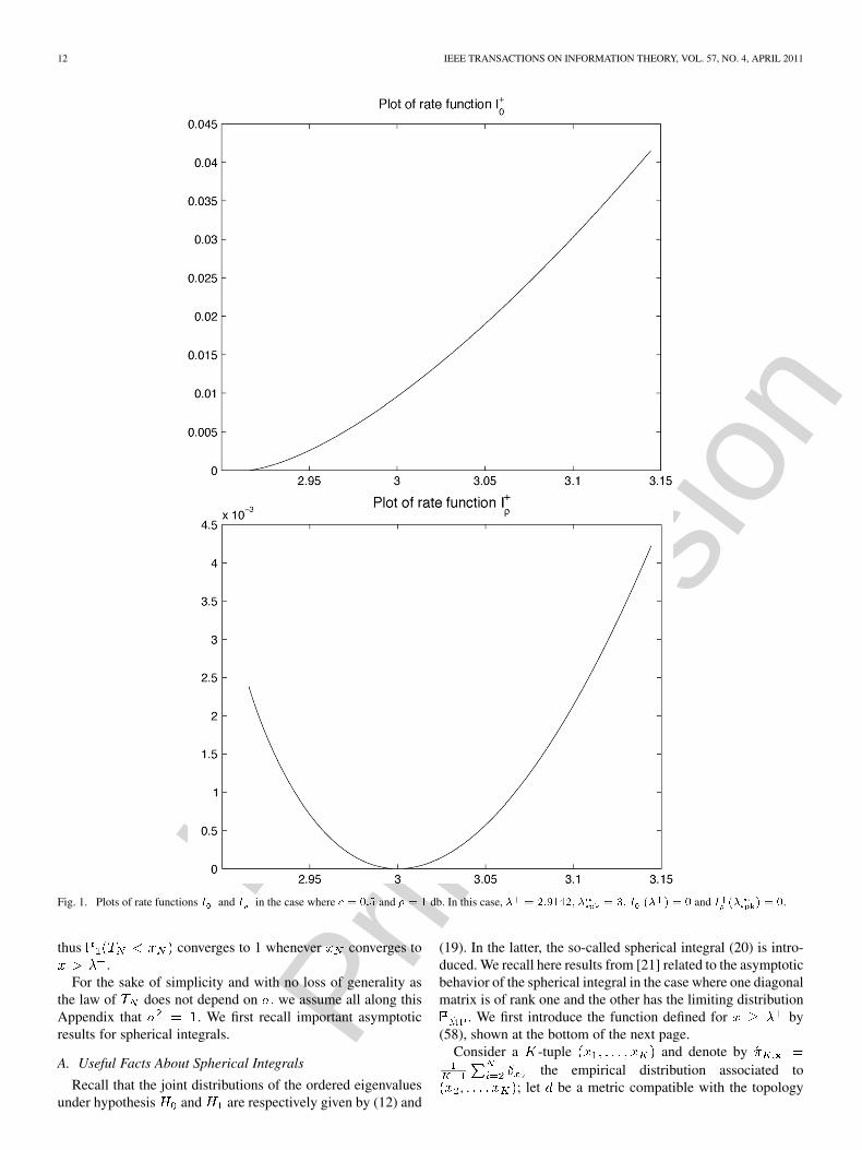
IEEE
Pro
of
Prin
t Ver
sion
12 IEEE TRANSACTIONS ON INFORMATION THEORY, VOL. 57, NO. 4, APRIL 2011
Fig. 1. Plots of rate functions � and � in the case where � � ��� and � � � db. In this case, � � ������� � � �� � � � � and � � � �.
thus converges to 1 whenever converges to.
For the sake of simplicity and with no loss of generality asthe law of does not depend on we assume all along thisAppendix that . We first recall important asymptoticresults for spherical integrals.
A. Useful Facts About Spherical Integrals
Recall that the joint distributions of the ordered eigenvaluesunder hypothesis and are respectively given by (12) and
(19). In the latter, the so-called spherical integral (20) is intro-duced. We recall here results from [21] related to the asymptoticbehavior of the spherical integral in the case where one diagonalmatrix is of rank one and the other has the limiting distribution
. We first introduce the function defined for by(58), shown at the bottom of the next page.
Consider a -tuple and denote bythe empirical distribution associated to
; let be a metric compatible with the topology
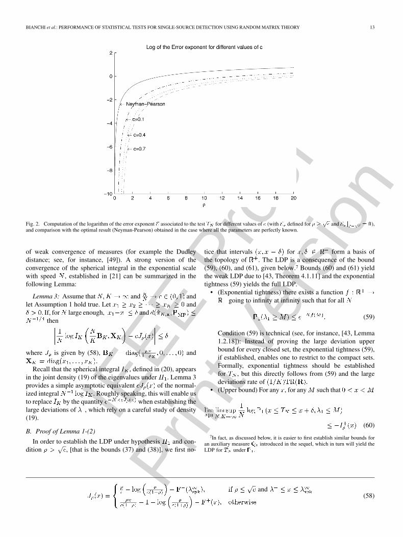
IEEE
Pro
of
Prin
t Ver
sion
BIANCHI et al.: PERFORMANCE OF STATISTICAL TESTS FOR SINGLE-SOURCE DETECTION USING RANDOM MATRIX THEORY 13
Fig. 2. Computation of the logarithm of the error exponent � associated to the test � for different values of � (with � defined for � � �� and � � � �),
and comparison with the optimal result (Neyman-Pearson) obtained in the case where all the parameters are perfectly known.
of weak convergence of measures (for example the Dudleydistance; see, for instance, [49]). A strong version of theconvergence of the spherical integral in the exponential scalewith speed , established in [21] can be summarized in thefollowing Lemma:
Lemma 3: Assume that and andlet Assumption 1 hold true. Let and
. If, for large enough, andthen
where is given by (58), and.
Recall that the spherical integral , defined in (20), appearsin the joint density (19) of the eigenvalues under . Lemma 3provides a simple asymptotic equivalent of the normal-ized integral . Roughly speaking, this will enable usto replace by the quantity when establishing thelarge deviations of , which rely on a careful study of density(19).
B. Proof of Lemma 1-(2)
In order to establish the LDP under hypothesis and con-dition , [that is the bounds (37) and (38)], we first no-
tice that intervals for form a basis ofthe topology of . The LDP is a consequence of the bound(59), (60), and (61), given below.7 Bounds (60) and (61) yieldthe weak LDP due to [43, Theorem 4.1.11] and the exponentialtightness (59) yields the full LDP.
• (Exponential tightness) there exists a functiongoing to infinity at infinity such that for all
(59)
Condition (59) is technical (see, for instance, [43, Lemma1.2.18]): Instead of proving the large deviation upperbound for every closed set, the exponential tightness (59),if established, enables one to restrict to the compact sets.Formally, exponential tightness should be establishedfor , but this directly follows from (59) and the largedeviations rate of
• (Upper bound) For any , for any such that
(60)
7In fact, as discussed below, it is easier to first establish similar bounds foran auxiliary measure introduced in the sequel, which in turn will yield theLDP for � under .
and(58)

IEEE
Pro
of
Prin
t Ver
sion
14 IEEE TRANSACTIONS ON INFORMATION THEORY, VOL. 57, NO. 4, APRIL 2011
Fig. 3. Error Exponent curves associated to the tests � �� � and � �� � in the case where � � and � � �� dB. Each point of the curve corresponds to agiven error exponent under � (� axis) and its counterpart error exponent under � (� axis) as described in Theorem 2-(2) for � and Theorem 3-(2) for � .
Fig. 4. Simulated ROC curves for � (test 1) and � (test 2) in the case where � � �� � �� and � � �� dB.
Due to the exponential tightness, it is sufficient to establishthe upper bound for compact sets. As each compact can becovered by a finite number of balls, it is, therefore, suffi-cient to establish upper estimate (60) in order to establishthe LD upper bound.
• (Lower bound) For any
(61)
The fact that (61) implies the LD lower bound (38) is stan-dard in LD and can be found in [43, Chapter 1], for in-stance.
As the arguments are very similar to the ones developed in [21],we only prove in detail the upper bound (60). Proofs of (59) and(61) are left to the reader.
The idea is that the empirical measure
(of all but the largest eigenvalues) and thetrace concentrate faster than the largest eigenvalue. In theexponential scale with speed and the trace can be

IEEE
Pro
of
Prin
t Ver
sion
BIANCHI et al.: PERFORMANCE OF STATISTICAL TESTS FOR SINGLE-SOURCE DETECTION USING RANDOM MATRIX THEORY 15
considered as equal to their limit, respectively and 1. Inparticular, the deviations of arise from those of the largesteigenvalue and they both satisfy the same LDP with the samerate function . We, therefore, isolate the terms depending on
and gather the others through their empirical measure .Recall the notations introduced in (12) and (19) and let
. Consider the following domain:
for large enough
where we performed the change of variables for, and the related modifications and
. Note also that strictlyspeaking, the domain of integration would be expressed dif-ferently with the ’s and in particular, we should have changedconstant which majorizes the ’s into a larger constant as the
’s can theoretically be slightly above —we keep the samenotation for the sake of simplicity.
To proceed, one has to study the asymptotic behavior of thenormalizing constant
which turns out to be difficult. Instead of establishing directlythe bounds (59)–(61), we proceed as in [21] and establish similarbounds replacing the probability measures by the measures
defined as
and the rate function by the function defined by
for . Notice that these positive measures are notprobability measures any more, and as a consequence, the func-tion is not necessarily positive and its infimum might not beequal to zero, as it is the case for a rate function.
Writing the upper bound for , we obtain
where, for any compactly supported probability measure andany real number greater than the right edge of the support of
Let us now localize the empirical measure around 8
and the trace around 1. The continuity and convergence proper-ties of the spherical integral recalled in Lemma 3 yield, forlarge enough
(62)
with
and
Note that the bounds of the first integral in (62) follow from thefact that the event implies that
provided that is satisfied.The second term in (62) is easily obtained considering the factthat all the eigenvalues are less than so that for
and .Now, standard concentration results under yield that
8Notice that if �� is close to , so is �� due to the change of variable� � � .

IEEE
Pro
of
Prin
t Ver
sion
16 IEEE TRANSACTIONS ON INFORMATION THEORY, VOL. 57, NO. 4, APRIL 2011
More precisely, one knows using [50] that the empirical measureis close enough to its expectation and then using
[51] one knows that the expectation is close enough to its limit. The arguments are detailed in the Wigner case in [21] and
we do not give more details here.As for is continuous
and is lower semi-continuous, we obtain
By continuity in of the two involved functions, we finally get
and the counterpart of (60) is proved for and function .The proof of the lower bound is quite similar and left to thereader. It remains now to recover (60). As is a probabilitymeasure and the whole space is both open and closed, anapplication of the upper and lower bounds for immediatelyyields
(63)
This implies that the LDP holds for with rate function.
It remains to check that , which easilyfollows from the fact to be proved that
(64)
We, therefore, study the variations of over . Notethat , and thus that
. Function being a Stieltjes transform is in-creasing for , and so is , whose limit at infinityis . Straightforward but involved computations usingthe explicit representation (67) for yield that .Therefore, is decreasing on and increasing on
, and (64) is proved.This concludes the proof of the upper bound in Lemma 1-(2).
The proof of Lemma 1-(1) is very similar and left to the reader.
C. Proof of Lemma 1-(3)
The proof of this point requires an extra argument as we studythe large deviations of near the point where therate function is not continuous. In particular, the limit (53) doesnot follow from the LDP already established. As we shall seewhen considering , the factthat the scale is the same as the one of the fluctuationsof the largest eigenvalue of the complex Wishart model is cru-cial.
We detail the proof in the case when and, as above,consider the positive measures . We need to prove that
(65)
the other bound being a direct consequence of the LDP. As pre-viously, we will carefully localize the various quantities of in-terest. Denote by forand by for . Notice also that
together with imply that. We shall also consider the further constraints:
and
which enable us to properly separate from the support of. Now, with the localization indicated above, we have for
large enough
As previously, we consider the variables forand obtain, with the help of Lemma 3
with

IEEE
Pro
of
Prin
t Ver
sion
BIANCHI et al.: PERFORMANCE OF STATISTICAL TESTS FOR SINGLE-SOURCE DETECTION USING RANDOM MATRIX THEORY 17
Therefore
(recall that ). Now, as, its
contribution vanishes at the LD scale
It remains to check that is boundedbelow uniformly in . This will yield the convergence of
towards zero; hence, (65). Con-sider
We have already used the fact that the first term goes tozero when grows to infinity. Recall that the fluctuationsof are of order ; therefore, the second termalso goes to zero as we consider deviations of order .Now, converges in distribution tothe Tracy–Widom law; therefore, the last term converges to
. This concludes the proof.
APPENDIX BSKETCH OF PROOF FOR LEMMA 2: LARGE DEVIATIONS FOR
As stated in Remark 10, we shall first study the LDP for thejoint quantity . The purpose here is to outline the fol-lowing convergence:
which is an illustrative way, although informal,9 to state the LDPfor [see (39)].
Consider the quantity . Aswe are interested in the deviations of and , the interestingscenario is and (recall thatare the edgepoints of the support of Marcenko–Pastur distribu-tion). More precisely, the interesting case is when the deviationsof the extreme eigenvalue occur outside of the bulk:and ; such deviations happen at the rate .The case where the deviations would occur within the bulk is
9All the statements, computations and approximations below can be madeprecise as in the proof of Lemma 1.
unlikely to happen because it would enforce the whole eigen-values to deviate from the limiting support of Marcenko–Pasturdistribution, which happens at the rate . Denote by
and
We shall now perform the following approximations:
The three first approximations follow from the fact that, the last one from Lemma 3.
Plugging these approximations into the expression ofyields

IEEE
Pro
of
Prin
t Ver
sion
18 IEEE TRANSACTIONS ON INFORMATION THEORY, VOL. 57, NO. 4, APRIL 2011
As and , the last integral goesto one as and
Recall that we are interested in the limit. The last term will account for a constant [see,
for instance, (63)]:
The term within the exponential in the integral ac-counts for the interraction between and and its contri-bution vanishes at the desired rate. In order to evaluate the tworemaining integrals, one has to rely on Laplace’s method (see,for instance, [52]) to express the leading term of the integrals(replacing by below)
Finally, we get the desired limit
where
It remains to replace by its expression (58) and to spreadthe constant over and , which are not a priori ratefunctions (recall that a rate function is nonnegative). If ,then the event is “typical” and no deviation occurs,otherwise stated, the rate function should satisfy
. Similarly, under and under
. Necessarily, should write under(resp. under ) and the rate functionsshould be given by:under (resp. under ), which are thedesired results.
We have proved (informally) that the LDP holds true forwith rate function . The contraction
principle [43, Chap. 4] immediatly yields the LDP for the ratiowith rate function
(66)
which is the desired result. We provide here intuitive argumentsto understand this fact.
For this, interpret the value of the rate function asthe cost associated to a deviation of (under ) around :
. If a deviation occurs forthe ratio , say where (which isthe typical behavior of under ), then necessarily mustdeviate around some value , so does around some value ,so that the ratio is around . In terms of rate functions, the costof the joint deviation is .The true cost associated to the deviation of the ratio will be theminimum cost among all these possible joint deviations ofand ; hence, the rate function (66).
APPENDIX CCLOSED-FORM EXPRESSIONS FOR FUNCTIONS AND
Consider the Stieltjes transform of Marcenko–Pastur distri-bution
We gather without proofs a few facts related to , which are partof the folklore.
Lemma 4 (Representation of ): The following hold true:1) Function is analytic in .2) If with , then
where stands for the principal branch of the square-root.
3) If with , then
where stands for the branch of the square-root whoseimage is .
4) As a consequence, the following hold true:
(67)
(68)

IEEE
Pro
of
Prin
t Ver
sion
BIANCHI et al.: PERFORMANCE OF STATISTICAL TESTS FOR SINGLE-SOURCE DETECTION USING RANDOM MATRIX THEORY 19
5) Consider the following function . Func-tions and satisfy the following system of equations:
(69)
Recall the definition (31) and (51) of function and .In the following lemma, we provide closed-form formulas ofinterest.
Lemma 5: The following identities hold true:1) Let then
2) Let then
Proof: Consider the case where . First write
Integrating with respect with and applying Funini’s the-orem yields
in the case where . Recall that and are holomorphicfunctions over and satisfy system (69)(notice in particular that and never vanish). Usingthe first equation of (69) implies that
(70)
Consider . By adirect computation of the derivative, we get
Hence
It remains to plug this identity into (70) to conclude. The repre-sentation of can be established similarly.
ACKNOWLEDGMENT
The authors would like to thank O. Cappé for many fruitfuldiscussions related to the GLRT.
REFERENCES
[1] J. Mitola, III and G. Q. Maguire, Jr., “Cognitive radio: Making soft-ware radios more personal,” IEEE Wireless Commun., vol. 6, pp. 13–18,1999.
[2] S. Haykin, “Cognitive radio: Brain-empowered wireless communica-tions,” IEEE J. Sel. Areas Commun., vol. 23, no. 2, pp. 201–220, Feb.2005.
[3] M. Dohler, E. Lefranc, and A. H. Aghvami, “Virtual antenna arraysfor future wireless mobile communication systems,” ICT. Beijing,China, 2002.
[4] H. Urkowitz, Energy Detection of Unknown Deterministic Signals, vol.55, no. 4, pp. 523–531, Apr. 1967.
[5] V. I. Kostylev, “Energy detection of a signal with random amplitude,”in Proc. IEEE Int. Conf. Communications, 2002, vol. 3, pp. 1606–1610.
[6] F. F. Digham, M.-S. Alouini, and M. K. Simon, “On the energy de-tection of unknown signals over fading channels,” in Proc. IEEE Int.Conf. Communications, May 2003, vol. 5, pp. 3575–3579.
[7] Z. Quan, S. Cui, A. H. Sayed, and H. V. Poor, “Spatial-spectral jointdetection for wideband spectrum sensing in cognitive radio networks,”presented at the ICASSP, Las Vegas, 2008.
[8] E. L. Lehman and J. P. Romano, Testing Statistical Hypotheses. NewYork: Springer, 2006, Springer Texts in Statistics.
[9] M. Wax and T. Kailath, “Detection of signals by information theoreticcriteria,” IEEE Trans. Signal, Speech, Signal Process., vol. 33, no. 2,pp. 387–392, Apr. 1985.
[10] P.-J. Chung, J. F. Bohme, C. F. Mecklenbrauker, and A. O. Hero, “De-tection of the number of signals using the Benjamini–Hochberg proce-dure,” IEEE Trans. Signal Process., vol. 55, no. 6, pp. 2497–2508, Jun.2007.
[11] A. Taherpour, M. Nasiri-Kenari, and S. Gazor, “Multiple antenna spec-trum sensing in cognitive radios,” IEEE Trans. Wireless Commun., vol.9, no. 2, pp. 814–823, 2010.
[12] X. Mestre, “Improved estimation of eigenvalues and eigenvectors ofcovariance matrices using their sample estimates,” IEEE Trans. Inf.Theory, vol. 54, no. 11, pp. 5113–5129, Nov. 2008.
[13] X. Mestre, “On the asymptotic behavior of the sample estimates ofeigenvalues and eigenvectors of covariance matrices,” IEEE Trans.Signal Process., vol. 56, no. 11, pp. 5353–5368, Nov. 2008.
[14] S. Kritchman and B. Nadler, “Determining the number of componentsin a factor model from limited noisy data,” Chemometrics and Intelli-gent Laboratory Systems, 2008, 1932, 94.
[15] S. Kritchman and B. Nadler, “Non-parametric detection of the numberof signals: Hypothesis testing and random matrix theory,” IEEE Trans.Signal Process., vol. 57, no. 10, pp. 3930–3941, Oct. 2009.
[16] J. Silverstein and P. Combettes, “Signal detection via spectral theoryof large dimensional random matrices,” IEEE Trans. Signal Process.,vol. 40, no. 8, pp. 2100–2105, Aug. 1992.
[17] R. Couillet and M. Debbah, “A Bayesian framework for collabo-rative multi-source signal detection,” IEEE Trans. Signal Process.,arxiv:0811.0764, to be published.
[18] N. R. Rao, J. A. Mingo, R. Speicher, and A. Edelman, “Statisticaleigen-inference from large Wishart matrices,” Ann. Statist., vol. 36, no.6, pp. 2850–2885, 2008.
[19] R. R. Nadakuditi and J. W. Silverstein, “Fundamental limit of samplegeneralized eigenvalue based detection of signals in noise using rela-tively few signal-bearing and noise-only samples,” IEEE J. Sel. TopicsSignal Process., vol. 4, no. 3, pp. 468–480, Jun. 2010.
[20] I. M. Johnstone, “On the distribution of the largest eigenvalue in prin-cipal components analysis,” Ann. Statist., vol. 29, no. 2, pp. 295–327,2001.
[21] M. Maida, “Large deviations for the largest eigenvalue of rank one de-formations of Gaussian ensembles,” Electron. J. Probab., vol. 12, pp.1131–1150, 2007, (electronic).
[22] Y. H. Zeng and Y. C. Liang, Eigenvalue Based Spectrum Sensing Al-gorithms for Cognitive Radio, Tech. Rep., 2008, arXiv:0804.2960v1.
[23] L. S. Cardoso, M. Debbah, P. Bianchi, and J. Najim, “Cooperative spec-trum sensing using random matrix theory,” in Proc. 3rd Int. Symp. Wire-less Pervasive Computing, May 2008, pp. 334–338.
[24] F. Penna, R. Garello, and M. Spirito, “Cooperative spectrum sensingbased on the limiting eigenvalue ratio distribution in Wishart matrices,”IEEE Commun. Lett., vol. 13, no. 7, pp. 507–509, Jul. 2009.

IEEE
Pro
of
Prin
t Ver
sion
20 IEEE TRANSACTIONS ON INFORMATION THEORY, VOL. 57, NO. 4, APRIL 2011
[25] T. Abbas, N.-K. Masoumeh, and G. Saeed, “Multiple antenna spec-trum sensing in cognitive radios,” IEEE Trans. Wireless Commun., tobe published.
[26] T. W. Anderson, “Asymptotic theory for principal component anal-ysis,” J. Math. Statist., vol. 34, pp. 122–148, 1963.
[27] A. W. van der Vaart, “Asymptotic statistics,” in Cambridge Series inStatistical and Probabilistic Mathematics. Cambridge, U.K.: Cam-bridge Univ. Press, 1998, vol. 3.
[28] M. L. Mehta, Random Matrices Volume 142 of Pure and Applied Math-ematics (Amsterdam), 3rd ed. Amsterdam, The Netherlands: Else-vier/Academic Press, 2004.
[29] G. Anderson, A. Guionnet, and O. Zeitouni, An Introduction toRandom Matrices. Cambridge, U.K.: Cambridge Univ. Press, 2009,Cambridge Studies in Advanced Mathematics.
[30] R. J. Muirhead, Aspects of Multivariate Statistical Theory, ser. WileySeries in Probability and Mathematical Statistics. Hoboken, NJ:Wiley, 1982.
[31] P. Koev, Random Matrix Statistics Toolbox [Online]. Available: http://math.mit.edu/plamen/software/rmsref.html
[32] P. Koev and A. Edelman, “The efficient evaluation of the hypergeo-metric function of a matrix argument,” Math. Comp., vol. 75, no. 254,pp. 833–846, 2006, (electronic).
[33] J. Mitola, “Cognitive Radio An Integrated Agent Architecture for Soft-ware Defined Radio,” Ph.D. dissertation, Royal Inst. Technol. (KTH),Stockholm, Sweden, May 2000.
[34] V. A. Marcenko and L. A. Pastur, “Distribution of eigenvalues in cer-tain sets of random matrices,” Mat. Sb. (N.S.), vol. 72, no. 114, pp.507–536, 1967.
[35] G. Ben Arous and A. Guionnet, “Large deviations for Wigner’s lawand Voiculescu’s non-commutative entropy,” Probab. Theory RelatedFields, vol. 108, no. 4, pp. 517–542, 1997.
[36] B. Nadler, “On the distribution of the ratio of the largest eigenvalue tothe trace of a wishart matrix,” Ann. Statist. [Online]. Available: http://www.wisdom.weizmann.ac.il/~nadler/ 2010
[37] C. A. Tracy and H. Widom, “Level-spacing distributions and the Airykernel,” Comm. Math. Phys., vol. 159, no. 1, pp. 151–174, 1994.
[38] C. A. Tracy and H. Widom, “On orthogonal and symplectic matrixensembles,” Comm. Math. Phys., vol. 177, no. 3, pp. 727–754, 1996.
[39] A. Bejan, “Largest eigenvalues and sample covariance matrices,”Tracy–Widom and Painleve II: Computational Aspects and Re-alization in S-Plus With Applications 2005 [Online]. Available:http://www.vitrum.md/andrew/TWinSplus.pdf
[40] F. Bornemann, “Asymptotic independence of the extreme eigenvaluesof Gaussian unitary ensemble,” J. Math. Phys., vol. 51, no. 2, p. 023514,8, 2010.
[41] J. Baik and J. Silverstein, “Eigenvalues of large sample covariance ma-trices of spiked population models,” J. Multivariate Anal., vol. 97, no.6, pp. 1382–1408, 2006.
[42] P. J. Bickel and P. W. Millar, “Uniform convergence of probabilitymeasures on classes of functions,” Statist. Sinica, vol. 2, no. 1, pp. 1–15,1992.
[43] A. Dembo and O. Zeitouni, Large Deviations Techniques and Applica-tions, 2nd ed. New York: Springer Verlag, 1998.
[44] Y. Q. Yin, Z. D. Bai, and P. R. Krishnaiah, “On the limit of thelargest eigenvalue of the large-dimensional sample covariance matrix,”Probab. Theory Related Fields, vol. 78, no. 4, pp. 509–521, 1988.
[45] Z. D. Bai and Y. Q. Yin, “Limit of the smallest eigenvalue of a large-dimensional sample covariance matrix,” Ann. Probab., vol. 21, no. 3,pp. 1275–1294, 1993.
[46] P. Bianchi, M. Debbah, and J. Najim, “Asymptotic independence inthe spectrum of the Gaussian unitary ensemble,” Electron. Commun.Probab. vol. 15, Sep. 2010, pp. 376–395.
[47] P.-N. Chen, “General formulas for the Neyman-Pearson type-II errorexponent subject to fixed and exponential type-i error bounds,” IEEETrans. Inf. Theory, vol. 42, no. 1, pp. 316–323, Jan. 1996.
[48] G. Ben Arous, A. Dembo, and A. Guionnet, “Aging of spherical spinglasses,” Probab. Theory Related Fields, vol. 120, no. 1, pp. 1–67,2001.
[49] R. M. Dudley, Real Analysis and Probability, Volume 74 of CambridgeStudies in Advanced Mathematics. Cambridge, U.K.: CambridgeUniv. Press, 2002, revised reprint of the 1989 original.
[50] A. Guionnet and O. Zeitouni, “Concentration of the spectral measurefor large matrices.,” Electron. Comm. Probab., vol. 5, pp. 119–136,2000, (electronic).
[51] Z. D. Bai, “Convergence rate of expected spectral distributions of largerandom matrices. II. Sample covariance matrices,” Ann. Probab., vol.21, no. 2, pp. 649–672, 1993.
[52] J. Dieudonné, Infinitesimal Calculus. Paris, France: Hermann, 1971,translated from French.
P. Bianchi was born in 1977 in Nancy, France. He received the M.Sc. degreefrom Supélec-Paris XI, France, in 2000, and the Ph.D. degree from the Univer-sity of Marne-la-Vallée, France, in 2003.
From 2003 to 2009, he was an Associate Professor with the Telecommuni-cation Department of Supélec. In 2009, he joined the Statistics and Applica-tions Group at LTCI-Telecom ParisTech. His current research interests are in thearea of statistical signal processing for sensor networks. They include decentral-ized detection, quantization, adaptive algorithms for distributed estimation, andrandom matrix theory.
M. Debbah was born in Madrid, Spain. He entered the Ecole NormaleSupérieure de Cachan, France, in 1996 where he received the M.Sc. and Ph.D.degrees in 1999 and 2002, respectively.
From 1999 to 2002, he was with Motorola Labs, working on wireless localarea networks and prospective fourth generation systems. From 2002 until 2003,he was appointed Senior Researcher at the Vienna Research Center for Telecom-munications (FTW) (Vienna, Austria). From 2003 until 2007, he was with theMobile Communications department of the Institut Eurecom (Sophia Antipolis,France) as an Assistant Professor. He is presently a Professor at Supélec (Gif-sur-Yvette, France), holder of the Alcatel-Lucent Chair on Flexible Radio. Hisresearch interests are in information theory, signal processing, and wireless com-munications.
Prof. Debbah is the recipient of the “Mario Boella” prize award in 2005, the2007 General Symposium IEEE GLOBECOM best paper award, the Wi-Opt2009 best paper award, the 2010 Newcom�� best paper award, as well asthe Valuetools 2007, Valuetools 2008, and CrownCom2009 best student paperawards. He is a WWRF fellow.
M. Maida received the Ph.D. degree from the Ecole normale supérieure, Lyon,France, in 2004.
She is a former student of the Ecole normale supérieure, Paris, France. Since2005, she has been an Associate Professor at the University Paris-Sud, Orsay.Her research interests include random matrices theory, large deviations, and freeprobability.
J. Najim received his engineering diploma from Télécom Paristech, France, in1998, and the Ph.D. degree from University Nanterre Paris-10 in 2001.
Since 2002, he has been with the Centre National de la Recherche Scien-tifique (CNRS) and Télécom Paristech. His research interests include wirelesscommunication, the theory of random matrices, and probability at large.