p hi ts · 2016-09-30 · 1 2 1 1 2
TRANSCRIPT

English version
PHITS
Ver. 2.88 User’s Manual

Contents
1 Introduction 11.1 Recent Improvements. . . . . . . . . . . . . . . . . . . . . . . . . . . . . . . . . . . . . . . . . 11.2 Development members. . . . . . . . . . . . . . . . . . . . . . . . . . . . . . . . . . . . . . . . 91.3 Reference of PHITS. . . . . . . . . . . . . . . . . . . . . . . . . . . . . . . . . . . . . . . . . . 9
2 Installation, compilation and execution of PHITS 112.1 Operating environment. . . . . . . . . . . . . . . . . . . . . . . . . . . . . . . . . . . . . . . . 112.2 Installation and execution on Windows. . . . . . . . . . . . . . . . . . . . . . . . . . . . . . . . 112.3 Installation and execution on Mac. . . . . . . . . . . . . . . . . . . . . . . . . . . . . . . . . . 122.4 Compilation using “make” command for Windows, Mac, and Linux. . . . . . . . . . . . . . . . 142.5 Compilation using Microsoft Visual Studio with Intel Fortran for Windows. . . . . . . . . . . . 152.6 Compilation of ANGEL . . . . . . . . . . . . . . . . . . . . . . . . . . . . . . . . . . . . . . . 162.7 Executable file . . . . . . . . . . . . . . . . . . . . . . . . . . . . . . . . . . . . . . . . . . . .162.8 Terminating the PHITS code. . . . . . . . . . . . . . . . . . . . . . . . . . . . . . . . . . . . . 162.9 Array sizes . . . . . . . . . . . . . . . . . . . . . . . . . . . . . . . . . . . . . . . . . . . . . .17
3 Input File 183.1 Sections. . . . . . . . . . . . . . . . . . . . . . . . . . . . . . . . . . . . . . . . . . . . . . . .183.2 Reading control. . . . . . . . . . . . . . . . . . . . . . . . . . . . . . . . . . . . . . . . . . . .193.3 Inserting files . . . . . . . . . . . . . . . . . . . . . . . . . . . . . . . . . . . . . . . . . . . . .203.4 User definition constant. . . . . . . . . . . . . . . . . . . . . . . . . . . . . . . . . . . . . . . . 203.5 Using mathematical expressions. . . . . . . . . . . . . . . . . . . . . . . . . . . . . . . . . . . 213.6 Particle identification. . . . . . . . . . . . . . . . . . . . . . . . . . . . . . . . . . . . . . . . . 22
4 Sections format 244.1 [ Title ] section . . . . . . . . . . . . . . . . . . . . . . . . . . . . . . . . . . . . . . . . . . . .244.2 [ Parameters ] section. . . . . . . . . . . . . . . . . . . . . . . . . . . . . . . . . . . . . . . . . 25
4.2.1 Calculation mode. . . . . . . . . . . . . . . . . . . . . . . . . . . . . . . . . . . . . . . 254.2.2 Number of history and Bank. . . . . . . . . . . . . . . . . . . . . . . . . . . . . . . . . 264.2.3 Cut off energy and switching energy. . . . . . . . . . . . . . . . . . . . . . . . . . . . . 284.2.4 Cut off time, cut off weight, and weight window. . . . . . . . . . . . . . . . . . . . . . . 304.2.5 Model option (1) . . . . . . . . . . . . . . . . . . . . . . . . . . . . . . . . . . . . . . . 314.2.6 Model option (2) . . . . . . . . . . . . . . . . . . . . . . . . . . . . . . . . . . . . . . . 324.2.7 Model option (3) . . . . . . . . . . . . . . . . . . . . . . . . . . . . . . . . . . . . . . . 334.2.8 Model option (4) . . . . . . . . . . . . . . . . . . . . . . . . . . . . . . . . . . . . . . . 344.2.9 Model option (5) . . . . . . . . . . . . . . . . . . . . . . . . . . . . . . . . . . . . . . . 354.2.10 Output options (1). . . . . . . . . . . . . . . . . . . . . . . . . . . . . . . . . . . . . . 354.2.11 Output options (2). . . . . . . . . . . . . . . . . . . . . . . . . . . . . . . . . . . . . . 374.2.12 Output option (3). . . . . . . . . . . . . . . . . . . . . . . . . . . . . . . . . . . . . . . 384.2.13 Output option (4). . . . . . . . . . . . . . . . . . . . . . . . . . . . . . . . . . . . . . . 394.2.14 Output option (5). . . . . . . . . . . . . . . . . . . . . . . . . . . . . . . . . . . . . . . 404.2.15 About geometrical errors. . . . . . . . . . . . . . . . . . . . . . . . . . . . . . . . . . . 414.2.16 Input-output file name. . . . . . . . . . . . . . . . . . . . . . . . . . . . . . . . . . . . 424.2.17 Others. . . . . . . . . . . . . . . . . . . . . . . . . . . . . . . . . . . . . . . . . . . . .424.2.18 Physical parameters for low energy neutron. . . . . . . . . . . . . . . . . . . . . . . . . 434.2.19 Physical parameters for photon and electron transport based on the original model. . . . 444.2.20 Parameters for EGS5. . . . . . . . . . . . . . . . . . . . . . . . . . . . . . . . . . . . . 454.2.21 Dumpall option. . . . . . . . . . . . . . . . . . . . . . . . . . . . . . . . . . . . . . . . 484.2.22 Event Generator Mode. . . . . . . . . . . . . . . . . . . . . . . . . . . . . . . . . . . . 52
4.3 [ Source ] section. . . . . . . . . . . . . . . . . . . . . . . . . . . . . . . . . . . . . . . . . . .534.3.1 <Source> : Multi-source . . . . . . . . . . . . . . . . . . . . . . . . . . . . . . . . . . . 544.3.2 Common parameters. . . . . . . . . . . . . . . . . . . . . . . . . . . . . . . . . . . . . 554.3.3 Cylinder distribution source. . . . . . . . . . . . . . . . . . . . . . . . . . . . . . . . . 574.3.4 Rectangular solid distribution source. . . . . . . . . . . . . . . . . . . . . . . . . . . . . 574.3.5 Gaussian distribution source (x,y,z independent). . . . . . . . . . . . . . . . . . . . . . 58
ii

4.3.6 Generic parabola distribution source (x,y,z independent). . . . . . . . . . . . . . . . . . 584.3.7 Gaussian distribution source (x-y plane). . . . . . . . . . . . . . . . . . . . . . . . . . . 594.3.8 Generic parabola distribution source (x-y plane). . . . . . . . . . . . . . . . . . . . . . . 594.3.9 Sphere and spherical shell distribution source. . . . . . . . . . . . . . . . . . . . . . . . 604.3.10 s-type= 11 . . . . . . . . . . . . . . . . . . . . . . . . . . . . . . . . . . . . . . . . . .614.3.11 s-type= 12 . . . . . . . . . . . . . . . . . . . . . . . . . . . . . . . . . . . . . . . . . .614.3.12 Cone shape. . . . . . . . . . . . . . . . . . . . . . . . . . . . . . . . . . . . . . . . . .624.3.13 Triangle prism shape. . . . . . . . . . . . . . . . . . . . . . . . . . . . . . . . . . . . . 634.3.14 Reading dump file. . . . . . . . . . . . . . . . . . . . . . . . . . . . . . . . . . . . . . 644.3.15 User definition source. . . . . . . . . . . . . . . . . . . . . . . . . . . . . . . . . . . . 674.3.16 Definition for energy distribution. . . . . . . . . . . . . . . . . . . . . . . . . . . . . . 704.3.17 Definition for angular distribution. . . . . . . . . . . . . . . . . . . . . . . . . . . . . . 784.3.18 Definition for time distribution. . . . . . . . . . . . . . . . . . . . . . . . . . . . . . . . 804.3.19 Example of multi-source. . . . . . . . . . . . . . . . . . . . . . . . . . . . . . . . . . . 834.3.20 Duct source option. . . . . . . . . . . . . . . . . . . . . . . . . . . . . . . . . . . . . . 87
4.4 [ Material ] section . . . . . . . . . . . . . . . . . . . . . . . . . . . . . . . . . . . . . . . . . .904.4.1 Formats. . . . . . . . . . . . . . . . . . . . . . . . . . . . . . . . . . . . . . . . . . . .904.4.2 Nuclide definition . . . . . . . . . . . . . . . . . . . . . . . . . . . . . . . . . . . . . . 904.4.3 Density definition. . . . . . . . . . . . . . . . . . . . . . . . . . . . . . . . . . . . . . . 914.4.4 Material parameters. . . . . . . . . . . . . . . . . . . . . . . . . . . . . . . . . . . . . 914.4.5 S(α, β) settings . . . . . . . . . . . . . . . . . . . . . . . . . . . . . . . . . . . . . . . . 914.4.6 Examples. . . . . . . . . . . . . . . . . . . . . . . . . . . . . . . . . . . . . . . . . . .92
4.5 [ Surface ] section. . . . . . . . . . . . . . . . . . . . . . . . . . . . . . . . . . . . . . . . . . .934.5.1 Formats. . . . . . . . . . . . . . . . . . . . . . . . . . . . . . . . . . . . . . . . . . . .934.5.2 Examples. . . . . . . . . . . . . . . . . . . . . . . . . . . . . . . . . . . . . . . . . . .934.5.3 Macro body. . . . . . . . . . . . . . . . . . . . . . . . . . . . . . . . . . . . . . . . . .954.5.4 Examples. . . . . . . . . . . . . . . . . . . . . . . . . . . . . . . . . . . . . . . . . . .964.5.5 Surface definition by macro body. . . . . . . . . . . . . . . . . . . . . . . . . . . . . . 97
4.6 [ Cell ] section. . . . . . . . . . . . . . . . . . . . . . . . . . . . . . . . . . . . . . . . . . . . .984.6.1 Formats. . . . . . . . . . . . . . . . . . . . . . . . . . . . . . . . . . . . . . . . . . . .984.6.2 Description of cell definition. . . . . . . . . . . . . . . . . . . . . . . . . . . . . . . . . 994.6.3 Universe frame. . . . . . . . . . . . . . . . . . . . . . . . . . . . . . . . . . . . . . . .1024.6.4 Lattice definition. . . . . . . . . . . . . . . . . . . . . . . . . . . . . . . . . . . . . . .1034.6.5 Repeated structures. . . . . . . . . . . . . . . . . . . . . . . . . . . . . . . . . . . . . .106
4.7 [ Transform ] section. . . . . . . . . . . . . . . . . . . . . . . . . . . . . . . . . . . . . . . . .1124.7.1 Formats. . . . . . . . . . . . . . . . . . . . . . . . . . . . . . . . . . . . . . . . . . . .1124.7.2 Mathematical definition of the transform. . . . . . . . . . . . . . . . . . . . . . . . . .1124.7.3 Examples (1). . . . . . . . . . . . . . . . . . . . . . . . . . . . . . . . . . . . . . . . .1134.7.4 Examples (2). . . . . . . . . . . . . . . . . . . . . . . . . . . . . . . . . . . . . . . . .113
4.8 [ Temperature ] section. . . . . . . . . . . . . . . . . . . . . . . . . . . . . . . . . . . . . . . .1144.9 [ Mat Time Change ] section. . . . . . . . . . . . . . . . . . . . . . . . . . . . . . . . . . . . .1154.10 [ Magnetic Field ] section. . . . . . . . . . . . . . . . . . . . . . . . . . . . . . . . . . . . . . .116
4.10.1 Charged particle. . . . . . . . . . . . . . . . . . . . . . . . . . . . . . . . . . . . . . .1164.10.2 Neutron. . . . . . . . . . . . . . . . . . . . . . . . . . . . . . . . . . . . . . . . . . . .117
4.11 [ Electro Magnetic Field ] section. . . . . . . . . . . . . . . . . . . . . . . . . . . . . . . . . .1184.12 [ Delta Ray ] section . . . . . . . . . . . . . . . . . . . . . . . . . . . . . . . . . . . . . . . . .1194.13 [ Super Mirror ] section. . . . . . . . . . . . . . . . . . . . . . . . . . . . . . . . . . . . . . . .1204.14 [ Elastic Option ] section. . . . . . . . . . . . . . . . . . . . . . . . . . . . . . . . . . . . . . .1214.15 [ Data Max ] section . . . . . . . . . . . . . . . . . . . . . . . . . . . . . . . . . . . . . . . . .1224.16 [ Frag Data ] section. . . . . . . . . . . . . . . . . . . . . . . . . . . . . . . . . . . . . . . . .1234.17 [ Importance ] section. . . . . . . . . . . . . . . . . . . . . . . . . . . . . . . . . . . . . . . . .1264.18 [ Weight Window ] section. . . . . . . . . . . . . . . . . . . . . . . . . . . . . . . . . . . . . .1274.19 [ Forced Collisions ] section. . . . . . . . . . . . . . . . . . . . . . . . . . . . . . . . . . . . .1284.20 [ Brems Bias ] section. . . . . . . . . . . . . . . . . . . . . . . . . . . . . . . . . . . . . . . . .1294.21 [ Photon Weight ] section. . . . . . . . . . . . . . . . . . . . . . . . . . . . . . . . . . . . . . .1304.22 [ Volume ] section. . . . . . . . . . . . . . . . . . . . . . . . . . . . . . . . . . . . . . . . . . .1314.23 [ Multiplier ] section . . . . . . . . . . . . . . . . . . . . . . . . . . . . . . . . . . . . . . . . .132
iii

4.24 [ Mat Name Color ] section. . . . . . . . . . . . . . . . . . . . . . . . . . . . . . . . . . . . . .1334.25 [ Reg Name ] section. . . . . . . . . . . . . . . . . . . . . . . . . . . . . . . . . . . . . . . . .1354.26 [ Counter ] section . . . . . . . . . . . . . . . . . . . . . . . . . . . . . . . . . . . . . . . . . .1364.27 [ Timer ] section. . . . . . . . . . . . . . . . . . . . . . . . . . . . . . . . . . . . . . . . . . . .137
5 Common parameters for tallies 1385.1 Geometrical mesh. . . . . . . . . . . . . . . . . . . . . . . . . . . . . . . . . . . . . . . . . . .138
5.1.1 Region mesh. . . . . . . . . . . . . . . . . . . . . . . . . . . . . . . . . . . . . . . . .1385.1.2 Definition of the region and volume for repeated structures and lattices. . . . . . . . . . 1395.1.3 r-z mesh. . . . . . . . . . . . . . . . . . . . . . . . . . . . . . . . . . . . . . . . . . . .1405.1.4 xyz mesh. . . . . . . . . . . . . . . . . . . . . . . . . . . . . . . . . . . . . . . . . . .141
5.2 Energy mesh . . . . . . . . . . . . . . . . . . . . . . . . . . . . . . . . . . . . . . . . . . . . .1415.3 LET mesh. . . . . . . . . . . . . . . . . . . . . . . . . . . . . . . . . . . . . . . . . . . . . . .1415.4 Time mesh. . . . . . . . . . . . . . . . . . . . . . . . . . . . . . . . . . . . . . . . . . . . . . .1425.5 Angle mesh. . . . . . . . . . . . . . . . . . . . . . . . . . . . . . . . . . . . . . . . . . . . . .1425.6 Mesh definition. . . . . . . . . . . . . . . . . . . . . . . . . . . . . . . . . . . . . . . . . . . .142
5.6.1 Mesh type. . . . . . . . . . . . . . . . . . . . . . . . . . . . . . . . . . . . . . . . . . .1425.6.2 e-type= 1 . . . . . . . . . . . . . . . . . . . . . . . . . . . . . . . . . . . . . . . . . . .1425.6.3 e-type= 2, 3 . . . . . . . . . . . . . . . . . . . . . . . . . . . . . . . . . . . . . . . . .1445.6.4 e-type= 4 . . . . . . . . . . . . . . . . . . . . . . . . . . . . . . . . . . . . . . . . . . .1445.6.5 e-type= 5 . . . . . . . . . . . . . . . . . . . . . . . . . . . . . . . . . . . . . . . . . . .144
5.7 Other tally definitions. . . . . . . . . . . . . . . . . . . . . . . . . . . . . . . . . . . . . . . . .1445.7.1 Particle definition. . . . . . . . . . . . . . . . . . . . . . . . . . . . . . . . . . . . . . .1445.7.2 axis definition. . . . . . . . . . . . . . . . . . . . . . . . . . . . . . . . . . . . . . . . .1455.7.3 file definition . . . . . . . . . . . . . . . . . . . . . . . . . . . . . . . . . . . . . . . . .1465.7.4 resfile definition . . . . . . . . . . . . . . . . . . . . . . . . . . . . . . . . . . . . . . .1465.7.5 unit definition. . . . . . . . . . . . . . . . . . . . . . . . . . . . . . . . . . . . . . . . .1465.7.6 factor definition. . . . . . . . . . . . . . . . . . . . . . . . . . . . . . . . . . . . . . . .1465.7.7 output definition . . . . . . . . . . . . . . . . . . . . . . . . . . . . . . . . . . . . . . .1475.7.8 info definition. . . . . . . . . . . . . . . . . . . . . . . . . . . . . . . . . . . . . . . . .1475.7.9 title definition. . . . . . . . . . . . . . . . . . . . . . . . . . . . . . . . . . . . . . . . .1475.7.10 ANGEL parameter definition. . . . . . . . . . . . . . . . . . . . . . . . . . . . . . . . .1475.7.11 2d-type definition. . . . . . . . . . . . . . . . . . . . . . . . . . . . . . . . . . . . . . .1485.7.12 gshow definition. . . . . . . . . . . . . . . . . . . . . . . . . . . . . . . . . . . . . . .1485.7.13 rshow definition . . . . . . . . . . . . . . . . . . . . . . . . . . . . . . . . . . . . . . .1495.7.14 x-txt, y-txt, z-txt definition. . . . . . . . . . . . . . . . . . . . . . . . . . . . . . . . . .1495.7.15 volmat definition. . . . . . . . . . . . . . . . . . . . . . . . . . . . . . . . . . . . . . .1505.7.16 epsout definition. . . . . . . . . . . . . . . . . . . . . . . . . . . . . . . . . . . . . . .1505.7.17 counter definition. . . . . . . . . . . . . . . . . . . . . . . . . . . . . . . . . . . . . . .1505.7.18 resolution and line thickness definitions. . . . . . . . . . . . . . . . . . . . . . . . . . .1505.7.19 trcl coordinate transformation. . . . . . . . . . . . . . . . . . . . . . . . . . . . . . . .1505.7.20 dump definition. . . . . . . . . . . . . . . . . . . . . . . . . . . . . . . . . . . . . . . .150
5.8 Function to sum up two (or more) tally results. . . . . . . . . . . . . . . . . . . . . . . . . . . .152
6 Tally input format 1546.1 [ T-Track ] section. . . . . . . . . . . . . . . . . . . . . . . . . . . . . . . . . . . . . . . . . . .1546.2 [ T-Cross ] section. . . . . . . . . . . . . . . . . . . . . . . . . . . . . . . . . . . . . . . . . . .1586.3 [ T-Point ] section. . . . . . . . . . . . . . . . . . . . . . . . . . . . . . . . . . . . . . . . . . .1636.4 [ T-Heat ] section . . . . . . . . . . . . . . . . . . . . . . . . . . . . . . . . . . . . . . . . . . .1666.5 [ T-Deposit ] section . . . . . . . . . . . . . . . . . . . . . . . . . . . . . . . . . . . . . . . . .1696.6 [ T-Deposit2 ] section. . . . . . . . . . . . . . . . . . . . . . . . . . . . . . . . . . . . . . . . .1736.7 [ T-Yield ] section. . . . . . . . . . . . . . . . . . . . . . . . . . . . . . . . . . . . . . . . . . .1756.8 [ T-Product ] section . . . . . . . . . . . . . . . . . . . . . . . . . . . . . . . . . . . . . . . . .1786.9 [ T-DPA ] section . . . . . . . . . . . . . . . . . . . . . . . . . . . . . . . . . . . . . . . . . . .1826.10 [ T-LET ] section . . . . . . . . . . . . . . . . . . . . . . . . . . . . . . . . . . . . . . . . . . .1856.11 [ T-SED ] section . . . . . . . . . . . . . . . . . . . . . . . . . . . . . . . . . . . . . . . . . . .1886.12 [ T-Time ] section. . . . . . . . . . . . . . . . . . . . . . . . . . . . . . . . . . . . . . . . . . .191
iv

6.13 [ T-Star ] section . . . . . . . . . . . . . . . . . . . . . . . . . . . . . . . . . . . . . . . . . . .1946.14 [ T - Dchain ] section. . . . . . . . . . . . . . . . . . . . . . . . . . . . . . . . . . . . . . . . .1976.15 [ T-WWG ] section . . . . . . . . . . . . . . . . . . . . . . . . . . . . . . . . . . . . . . . . . .2016.16 [ T-Userdefined ] section. . . . . . . . . . . . . . . . . . . . . . . . . . . . . . . . . . . . . . .2036.17 [ T-Gshow ] section. . . . . . . . . . . . . . . . . . . . . . . . . . . . . . . . . . . . . . . . . .2076.18 [ T-Rshow ] section. . . . . . . . . . . . . . . . . . . . . . . . . . . . . . . . . . . . . . . . . .2096.19 [ T-3Dshow ] section. . . . . . . . . . . . . . . . . . . . . . . . . . . . . . . . . . . . . . . . .211
6.19.1 box definition. . . . . . . . . . . . . . . . . . . . . . . . . . . . . . . . . . . . . . . . .2146.19.2 3dshow example. . . . . . . . . . . . . . . . . . . . . . . . . . . . . . . . . . . . . . .215
7 Volume and Area calculation by tally function 218
8 Processing dump file 220
9 Output cutoff data format 224
10 Region error check 225
11 Additional explanation for the parallel computing 22611.1 Distributed memory parallel computing. . . . . . . . . . . . . . . . . . . . . . . . . . . . . . .226
11.1.1 How to execute. . . . . . . . . . . . . . . . . . . . . . . . . . . . . . . . . . . . . . . .22611.1.2 Adjustment of maxcas and maxbch. . . . . . . . . . . . . . . . . . . . . . . . . . . . .22611.1.3 Treatment of abnormal end. . . . . . . . . . . . . . . . . . . . . . . . . . . . . . . . . .22611.1.4 ncut, gcut, pcut and dumpall file definition in the PHITS. . . . . . . . . . . . . . . . . . 22711.1.5 Read in file definition in the PHITS. . . . . . . . . . . . . . . . . . . . . . . . . . . . .227
11.2 Shared memory parallel computing. . . . . . . . . . . . . . . . . . . . . . . . . . . . . . . . . .22711.2.1 Execution. . . . . . . . . . . . . . . . . . . . . . . . . . . . . . . . . . . . . . . . . . .22711.2.2 Important notices for shared memory parallel computing. . . . . . . . . . . . . . . . . . 228
12 FAQ 22912.1 Questions related to parameter setting. . . . . . . . . . . . . . . . . . . . . . . . . . . . . . . .22912.2 Questions related to error occurred in compiling or executing PHITS. . . . . . . . . . . . . . . . 23012.3 Questions related to Tally. . . . . . . . . . . . . . . . . . . . . . . . . . . . . . . . . . . . . . .23012.4 Questions related to source generation. . . . . . . . . . . . . . . . . . . . . . . . . . . . . . . .231
13 Concluding remarks 232
index 234
v

1
1 Introduction
Particle and heavy ion transport code is an essential implement in design and study of spacecrafts and accel-erator facilities. We have therefore developed the multi-purpose Monte Carlo Particle and Heavy Ion Transportcode System,PHITS ,1, 2) based on the NMTC/JAM.3) The physical processes which we should deal with in amultipurpose simulation code can be divided into two categories, transport process and collision process. In thetransport process, PHITS can simulate a motion under external fields such as magnetic and gravity. Without theexternal fields, neutral particles move along a straight trajectory with constant energy up to the next collision point.However, charged particles and heavy ions interact many times with electrons in the material losing energy andchanging direction. PHITS treats ionization processes not as collision but as a transport process under an externalfield. The averagedE/dx is given by the charge density of the material and the momentum of the particle takinginto account the fluctuations of the energy loss and the angular deviation. The second category of the physicalprocesses is the collision with the nucleus in the material. In addition to the collision, we consider the decay of theparticle as a process in this category. The total reaction cross section, or the life time of the particle is an essentialquantity in the determination of the mean free path of the transport particle. According to the mean free path,PHITS chooses the next collision point using the Monte Carlo method. To generate the secondary particles of thecollision, we need the information on the final states of the collision. For neutron induced reactions in low energyregion, PHITS employs the cross sections from Evaluated Nuclear Data libraries. For high energy neutrons andother particles, we have incorporated two models, JAM4) and JQMD5) to simulate the particle induced reactionsup to 200 GeV and the nucleus-nucleus collisions, respectively.
RecentlyPHITS introduces an event generator for particle transport parts in the low energy region. Thus,PHITS was completely rewritten for the introduction of the event generator for neutron-induced reactions in energyregion less than 20 MeV. Furthermore, several new tallis were incorporated for estimation of the relative biologicaleffects. This report includes descriptions on new features and functions introduced into the code. For examples,GG geometry, parallelization, DPA tally, neutron, photon and electron transportation, and detailed descriptionshow to setup the geometry as well. In order to keep comprehensive descriptions as the manual ofPHITS , thisreport includes description on some parts of the NMTC/JAM code, which is an origin of code structure ofPHITS .
1.1 Recent Improvements
Essences of improvements after version 2.24 are described below.
From version 2.88, following functions were implemented.
• The sumtally function became applicable to[t-dchain] tally.
• Two options of the function about user defined cross sections were developed. One is an extrapolationfunction to extrapolate given data for incident energies, emission angles, and emission energies. The other iseffective in the case that there are no data of differential cross section. You can use nuclear reaction modelsto simulate nuclear reaction events only with data of total reaction cross section.
• Bug that all neutrons with lower energy thanemin(2) decay was fixed. (From ver. 2.83, this bug occurred.)
From version 2.87, following functions were implemented.
• The arrows to indicate the xyz coordinates are depicted in[t-3dshow] tally.
• Calculation algorithm for tetrahedral geometry was revised to reduce the computational time.
• The file name of geometry-error information file (“*.err” ) was changed to (“*geo.out” )
• Bug in the use of MTx, i.e.S(α, β) table, in[material] section was fixed. This bug occurred only inversion 2.86.
From version 2.86, following functions were implemented.
• A new tally [t-wwg] was introduced. Using this tally, you can automatically determine an appropriatesetting for the[Weight Window] section. See Section6.15in more detail.

2 1 INTRODUCTION
• A function to output the tally results in xyz-mesh in the input format of ParaView, which is an open-source, multi-platform data analysis and visualization application, was implemented. See documents in\utility\ParaView folder in more detail. Furthermore, a function to generate Bitmap figure of 2-dimensionaltally output was implemented. These improvements were performed under supports of Dr. Furutaka of Re-search Group for Nuclear Sensing, JAEA, and V.I.C., Inc.
• A new mode for calculating stopping power of all charged particle by ATIMA,ndedx = 3, was added, andset as the default value.
• The name of file to output the current batch information was changed frombatch.now to batch.out. Youcan specify this file name by settingfile(22) in [parameters] section.
• The RI-source function was implemented. Using this function, PHITS can generate photon sources withenergy spectra of radioisotope (RI) decay by simply specifying the activity and name of the RIs. Nucleardecay database DECDC1 was used in this function. This database is equivalent to ICRP107. See Table4.50in more detail. This improvement was performed under support of Dr. A. Endo of Japan Atomic EnergyAgency (JAEA).
• A new parameternaturalwas introduced. When you define an element without specifying its mass numberin [material] section, and setnatural = 1 or 2, PHITS assumes that it has natural isotope composition.Note that natural isotopes whose nuclear data are not included in JENDL-4.0 are ignored in the calculation.This improvement was performed under support of Center for Computational Science & e-Systems, JAEA.
• A new section[Data Max]was introduced to specify thedmax parameter for each nucleus and material. SeeSection4.15in more detail. This improvement was performed under support of Center for ComputationalScience & e-Systems, JAEA.
• Muon nuclear reaction model was improved. See this paper2 in more detail.
• A new model for deuteron-nucleus total reaction cross sections was introduced. This model can be used bysettingicrdm=1 in [parameters] section. See this paper3 in more detail.
• The pion total reaction cross section model was improved, and employed as the default model. The improvedmodel reproduces experimental data of the cross sections better than the old model, which uses geometricalformula. You can select the models byicxspi parameter.
• Several sumtally subsection can be defined in an input. Some bugs were fixed related to sumtally.
From version 2.85, following functions were implemented.
• High-energy heavy ion reaction model, JAMQMD, which works above 3 GeV/u, was improved to JAMQMD2,in the same manner as JQMD. The accuracy as well as the stability of the calculation are improved, particu-larly for cosmic-ray simulation.
• Algorithm of stopping power calculation ATIMA in PHITS was improved. PHITS simulation with highprecision ATIMA is now possible in the almost same calculation time with SPAR by this improvement.This improvement was performed by Mr. Akio Wada of Research Organization for Information Science &Technology (RIST), and was supported by Center for Computational Science & e-Systems, Japan AtomicEnergy Agency (JAEA).
• The unit ofesmin andesmax parameters is changed from MeV to MeV/u. These parameters define theminimum and maximum energy of charged particles treated in the simulation, respectively.
• A bug in the high-energy photon transport (approximately above 10 MeV) using EGS5 mode was fixed.
• A bug in the capture reaction of negative muon when1H is included in the material was fixed.
1 A. Endo, Y. Yamaguchi and K.F. Eckerman, Nuclear decay data for dosimetry calculation - Revised data of ICRP Publication 38, JAERI1347 (2005).
2 S. Abe and T. Sato, Implementation of muon interaction models in PHITS, J. Nucl. Sci. Technol. (2016)[http://www.tandfonline.com/doi/abs/10.1080/00223131.2016.1210043]
3 K. Minomo, K. Washiyama, and K. Ogata, J. Nucl. Sci. Tech. DOI:10.1080/00223131.2016.1213672

1.1 Recent Improvements 3
From ver. 2.84, some bugs were fixed.
From version 2.83, following functions were implemented.
• Neutron decay can be considered. Mean life time of neutron is approximately 886.7 sec. Thus, you have toset a very large value fortmax (default= 1.0e9 ns) when you would like to consider neutron decay in yoursimulation.
• Bug in the treatment of the Doppler effect using the EGS5 mode was fixed. Due to this bug, previous versionsof PHITS scored some energies for[t-deposit] with part = photon, which should have been 0.
• A bug in[t-point] was fixed. This bug occurred when you write other tallies withmesh = reg behind a[t-point] tally, and might cause the results of the other tallies to be wrong.
• We fixed a bug that thesumtally function doesn’t work in an input file includinginfl.
From version 2.82, following functions were implemented.
• Point estimator tally[t-point] was implemented to calculate the particle fluence at a certain point or ring(see section6.3as well as\utility\tpoint folder)
• A new parameterelastic was added in[t-yield] tally to output recoil nucleus from elastic scattering.
• A new output optiontransmut was added in[t-star] tally to output star density for a reaction whichinduces transmutation of target nucleus.
• A new optionfiss was added in[counter] section to output the information on secondary particles gen-erated through fission reaction, particularly in each generation of sequential fissions.
• A new function was implemented in[source] section to generate neutron sources from spontaneous fission.In this function, the multiplicity of neutron and its energy spectrum are taken from Ref.4. See section4.3.2in more detail. The PHITS development team is grateful to Dr. Liem Peng Hong of NAIS, Co., Inc. for hissupport on developing the function.
• A new function was implemented in[source] section to generate particles from a triangle prism. Seesection4.3.13in more detail.
• A new function was implemented in[source] section to generate particles with arbitrary time information.See section4.3.18in more detail.
• A new parameterNONU was added in[parameters] section to control the neutron multiplicity.
• A new function to calculate the particle fluence in sector prisms was implemented in[t-track] tally byintroducingθ mesh in the case ofmesh = r-z.
• Some bugs in the EGS5 algorithm were fixed.
• A new function to consider the polarization of photon was implemented in the calculation of nuclear flores-cence resonance (NRF).
• Restart calculation using[t-dpa] tally became feasible.
• Sum tally function became applicable to all tallies except for[t-dchain]. (From ver. 2.88, this functionbecame applicable to all tallies.)
• Contribution of each particle can be properly calculated using[t-deposit] with output = depositoption.
• Some bugs in the muon- and photon-induced nuclear reaction models as well as JQMD-2.0 were fixed.
• Instructions how to use tetrahedral geometry (TetraGEOM), point estimator tally (tpoint), and user-definedtally (usrtally) were added in theutility folder.
4 J. M. Verbeke, C. Hagmnn, and D. Wright, “Simulation of Neutron and Gamma Ray Emission from Fission and Photofission”, UCRL-AR-228518 (2014).

4 1 INTRODUCTION
From version 2.81, following functions were implemented.
• We revisedmakefile to consider the dependence of each source file. Owning to this improvement, you canusemake -j option to speed up the compilation of PHITS. Please be careful that the target (executable) filename was changed in the revised makefile. This revision was performed under support of Dr. Furutaka ofResearch Group for Nuclear Sensing, JAEA.
• The limitation of the number of material when you use EGS5 was eliminated. However, PHITS calculationmay crash due to insufficient memory when you define more than a few hundred materials. In addition, themaximum number of elements per one material is still limited to 20.
• We fixed bugs in[t-track] and[t-deposit] when you use EGS5.
• We fixed a bug in[t-dchain] to properly consider the successive lines. The maximum number of regionsthat can be specified in[t-dchain] was extended up to 500.
• We fixed a bug in[t-deposit], mesh=reg, output=deposit when you use[delta-ray] section.
• We fixed a bug in[t-heat] with mesh=r-z.
From version 2.80, following functions were implemented.
• The function to read tetrahedral geometry (a kind of polygonal geometry) was implemented (see section4.6.5). This implementation was carried out under support of HUREL, Hanyang University, Korea.
• The function to produce bremsstrahlung and electron-positron pair by muon interaction was implemented.
• The function for simulating nuclear resonance florescence (NRF) was implemented. This function enables toreproduce the excitation of nucleus and the associate production of isomer by lower energy photon. Nuclearresonance fluorescence model can be activated by settingipnint=2 in the[parameters] section.
• “Sum” tally function became applicable to all tallies except for[t-dpa] and[t-dchain].
• The function to read user defined cross sections was implemented (see Section4.16)
• Algorithm to consider energy straggling of charged particles was revised to reproduce the doses aroundBragg peak more precisely.
• A new parameteridelt was introduced to reduce the computational time for particle transport simulationin very large gas area. Whenidelt=1, deltm anddeltc are divided by the density of each material.
• The function to properly calculate the uncertainty of tally results was implemented in the case of using“dump” source (see Section4.3.14).
• A new parameterpnimul was introduced to bias the photo-nuclear reaction cross section against photo-atomic interaction cross section.
• Bug in the calculation of the uncertainty of[t-yield] was fixed
• Improvements related to EGS5 mode
– A new parameteripegs was introduced to control PEGS5 execution before PHITS simulation.
– A new parameterimsegswas introduced to precisely simulate the multiple scattering of electron everytime when electron goes into a new material. This is an original option only in PHITS (not in theoriginal EGS5).
– A bug in the electron transport algorithm only in PHITS2.77 (not PHITS 2.76 or before) was fixed.Due to this bug, the range of electrons calculated by PHITS2.77 was too short.
– The limitation of the number of material used in PHITS was eliminated even using EGS5.
From version 2.77, following functions were implemented.
• We fixed a bug that unnatural energy distribution is tallied with settingaxis=eng when EGS5 is used.
• Muon-nuclear interaction model about muon capture reaction was revised.

1.1 Recent Improvements 5
• We changed the default setting of the nuclear reaction model in the case that light ions are targets. Whensuch a reaction occurs, PHITS calculates it with regarding the light ions as projectile on the basis of theinverse kinematics. For example, in the default setting, INCL is used even for heavy ion induced reactionswhen deuteron is set to be its target nucleus.
From version 2.76, following functions were implemented.
• Muon-nuclear interaction model based on the virtual photon production theory was implemented. Char-acteristic X-ray production from muonic atoms as well as associating muon capture reaction can be alsoconsidered in the new version.
• Adjustment parameters for determing the magnitude of angular straggling fornspred = 2were introduced.
• Bugs due to the problem of Intel Fortran 2015 were fixed.
From ver. 2.75, we fixed a bug that the function of sum tally does not work when you use an input file includingsome sections of tally, and corrected a bug occurs in settinge-mode=2.
From version 2.74, following functions were implemented.
• Version of DCHAIN-SP included in the PHITS package was changed from DCHAIN-SP2001 (dchain264.exe)to DCHAIN-SP2014 (dchain274.exe). DCHAIN-SP2014 was improved from DCHAIN-SP2001 in terms ofthe following aspects;
(1) The input format was changed.
(2) The number of energy groups of neutron activation cross section libraries was increased from 175 to1968.
(3) A new function was implemented to output the [source] section of PHITS from the activities calculatedby DCHAIN-SP.
(4) A new function was implemented to output the time dependence of radioactivities in each region in theinput format of ANGEL.
• Thread parallelization is available even using EGS5, i.e.negs = 1. Some bugs related to EGS5 were fixed.This improvement was performed by Mr. Masaaki Adachi of Research Organization for Information Science& Technology (RIST), and was supported by Center for Computational Science & e-Systems, Japan AtomicEnergy Agency (JAEA).
• A new function to combine two (or more) tally results, named “sum tally”, was implemented. (From ver.2.88, this function became applicable to all tallies.) See Sec.5.8in more detail. This function was developedby Mr. Takamitsu Miura of RIST, and was supported by Center for Computational Science & e-Systems,JAEA.
• The Kurotama model was revised to be capable of calculating the cross sections over 5 GeV/u. See thisarticle5 in more detail.
• The gamma de-excitation data contained intrxcrd.datwas incorporated in the source files of PHITS. Con-sequently,file(14) parameter is not necessary to be specified in PHITS input file even settinge-mode≥1or igamma≥1.
• Some bugs related to JAM and JAMQMD etc. were revised.
From ver. 2.73, we fixed a bug producing abnormal nuclei such as di-neutron in calculation of nuclear reactionmodels. For Windows, an installed executable file of the OpenMP version is available only on 64-bit. You canexecutePHITS in single processing on both the 32-bit and 64-bit systems, but you cannot do it using OpenMP on32-bit.
From ver. 2.72, we fixed a bug occurs in settingigamma=2, and corrected an error that the GEM modelproduces di-neutron. An error of angular distribution defined by degree in[source] section usinga-type was
5 L. Sihveret al., Nucl. Instr. & Meth. B 334, 34-39 (2014).

6 1 INTRODUCTION
corrected. In the former version, because of an incorrect interpolation, a biased distribution was used when you setthea-type sub-section using degree. Furthermore, we changed the definition ofna andnn in [source] sectionusinga-type. You cannot set these parameters to be negative.
From ver. 2.71, we fixed a bug about electron-positron annihilation occurred when EGS5 was used.
From ver. 2.70, the following functions were implemented.
• Transport algorithm for photons, electrons and positions in EGS5 (Electron Gamma Shower Version 56 ) wasincorporated. You can use this algorithm instead of the original one by settingnegs = 1 in [parameters]section. In addition,file(20)must be specified. At this moment, you cannot setnegs = 1 in the OpenMPversion ofPHITS . The maximum number of material is limited to 100 whennegs = 1. (From ver. 2.80,there is no this limitation.) See Sec.4.2.20in detail. This improvement was supported by Dr. Hirayamaand Dr. Namito of KEK.
• High-energy photo-nuclear reaction can be treated up to 1 TeV by implementing non-resonant photo-nuclearreaction mechanism in JAM.
• Muon-induced nuclear reaction can be treated up to 1 TeV by considering the generation of virtual photonfrom muon. You can activate this model by settingimuint = 1 in [parameters] section.
• The event generator mode ver.2 was improved to precisely determine the charged particle spectra on thebasis of their cross section data such as (n, p) and (n, α) contained in evaluated nuclear data library. You canuse this new event generator mode by settinge-mode=2 in [parameters] section.
• JQMD was improved to consider the relativistic effect. The algorithm for stabilizing the initial state ofnucleus was also implemented. The improved JQMD, named JQMD-2.0, can be activated by settingirqmd
= 1 in [parameters] section. This improvement was performed under collaboration with Dr. D. Mancusiat CEA/Saclay.
• Detector resolution can be considered in the event-by-event deposition energy calculation using[t-deposit]
with output = deposit.
From ver. 2.67, the following functions were implemented.
• A geometry check function was implemented. This function works when you specify a tally for generatingthe two-dimensional view of your geometry. When double defined or undefined regions are detected, theirregions are painted on the two-dimensional view. See Sec.10 in detail.
• An extension of the event generator mode (ver.2) was implemented. Owing to this implementation, theaccuracy of event-by-event analysis for the reactions induced by neutrons below 20 MeV was improved. SeeSec.4.2.22in detail.
• New parameterinfout was added to control output information infile(6) (D=phits.out). You canselect the information that you need.
• The current batch number appears on the console window in real time. Some important error and warningmessages such as “input data file for cross section directory does not exist.” are also shown in the window.
• Cone shape can be used for specifying the source locations by settings-type=18, 19.
• Dumpall anddump function for[t-cross], [t-time], [t-product] tallies can be used in the restartcalculation. For this revision, the rule for specifying the file names was changed. Results written in aconfiguration file (.cfg) in the former version of PHITS (before 2.66) are outputted in a file specified by“file=***”. Dump data are outputted in another file named “***dmp”.
• We increased the total memory usage ofPHITS (mdas) given in theparam.inc file to 120,000,000 (equiv-alent to 1GB), and the maximum number of lattice in a cell to 25,000,000. By this extention, we can use adetailed voxel phantom such as ICRP phantom without recompiling the source code.
From ver. 2.66, the following functions were implemented.6 H. Hirayamaet al., SLAC-R-730 (2005) and KEK Report 2005-8 (2005).

1.1 Recent Improvements 7
• Algorithm for including discrete spectra calculated by DWBA (Distorted Wave Born Approximation) wasimplemented. In several nuclear reactions induced by protons or deuterons, discrete peaks are added toneutron and proton spectra obtained by nuclear reaction models.
• Pion production processes in photo-nuclear reactions were included by implementing∆ andN∗ resonances.Thus, PHITS2.66 can treat the photo-nuclear reaction up to 1 GeV.(From ver. 2.70, this model is availableup to 1 TeV.)
• Results in the unit of Gy can be also obtained in[t-heat] tally. We corrected a bug thatNaN was detectedin the case of void regions.
• We fixed a bug occurred when you setnm to be negative in[source] section usinge-type = 2,3,5,6,7,12,15,16, which specify the energy spectrum by functional shape. Furthermore, we also fixed the similarbug fornn in the cases ofa-type = 5,6,15,16, which specify the angular distribution by the shape.
From ver. 2.65, dose in the unit of Gy can be obtained in[t-deposit] tally. Furthermore, a bug in convertingmass density to particle density in [material] and [cell] sections was fixed. This bug caused errors (0.6% at themost) in calculated results, when neutron-rich nuclei were used.
From ver. 2.64, bugs in photo-nuclear reaction model and EBITEM, and other minor bugs were fixed. Fur-thermore,NaN was detected in[T-Heat] calculations because of negative values in the probability table (p-table).The Ace libraries were re-produced by neglecting p-tables for the following 130 nuclides:
As075 Ba130 Ba132 Ba134 Ba135 Ba136 Ba137 Ba140 Br079 Br081 Cd106 Cd108
Cd110 Cd111 Cd112 Cd113 Cd114 Cd116 Ce141 Ce142 Ce143 Ce144 Cf250 Fe059
Ga069 Ga071 Hf174 Hf176 Hf177 Hf178 Hf179 Hf180 Hf181 Hf182 I_127 I_129
I_130 I_131 I_135 In113 In115 Kr078 Kr080 Kr082 Kr083 Kr084 Kr085 La138
La139 La140 Mo092 Mo094 Mo095 Mo096 Mo097 Mo098 Mo099 Mo100 Nb094 Nb095
Ni059 Pr141 Pr143 Rb085 Rb086 Rb087 Rh103 Rh105 Ru096 Ru098 Ru099 Ru100
Ru101 Ru102 Ru103 Ru104 Ru105 Ru106 Sb121 Sb123 Sb124 Sb125 Sb126 Se074
Se076 Se077 Se078 Se079 Se080 Se082 Sr084 Sr086 Sr087 Sr088 Sr089 Sr090
Tc099 Te120 Te122 Te123 Te124 Te125 Te126 Te127m Te128 Te129m Te130 Te132
Xe124 Xe126 Xe128 Xe129 Xe130 Xe131 Xe132 Xe133 Xe134 Xe135 Y_089 Y_090
Y_091 Yb168 Yb170 Yb171 Yb172 Yb173 Yb174 Yb176 Zr093 Zr095
From ver. 2.60, the following functions are implemented.
• Algorithm for de-excitation of nucleus after the evaporation process was improved by implementing EBITEM(ENSDF-Based Isomeric Transition and isomEr production Model). Prompt gamma spectrum can be pre-cisely estimated, including discrete peaks. The isomer production rates can be properly estimated.
• Quasi-deuteron disintegration, which is the dominant photo-nuclear mechanism between 25 to 140 MeV,was implemented in JQMD. Thus, PHITS2.60 can treat the photo-nuclear reaction up to 140 MeV.(Fromver. 2.70, this model is available up to 1 TeV.)The evaporation process after the giant resonance of6Li, 12C,14N, 16O was improved by considering the isospin of excited nucleus. Thus the alpha emission is suppressedand neutron and proton emission is enhanced from the giant resonance of these nuclei.
• Particle transport simulation in the combination field of electro-magnetic fields became available. See4.11section in detail.
• New energy mesh functions were implemented in[source] section in order to directly define differentialenergy spectrum in (/MeV) as well as discrete energy spectrum.
• Several algorithms were optimized to reduce the computational time, especially forxyz mesh tally withistdev = 2. Furthermore, use of memory for tally andANGEL was improved. These improvement wereperformed by Mr. Daichi Obinata of Fujitsu Systems East Limited, and were supported by Center forComputational Science & e-Systems, Japan Atomic Energy Agency (JAEA).
• Minor revision and bug fix.
– Number of cells acceptable in[t-dchain] was increased.
– The references ofPHITS and INCL were changed.

8 1 INTRODUCTION
– 7-digit cell ID became acceptable.
– Maximumdmax for electron and positron was changed from 1 GeV to 10 GeV.
– Restart calculation became available even whenPHITS did not stop properly.
– Lattice cell became acceptable in[t-dchain].
– Avoid the termination ofPHITS when some strange error occurs in JAM.
– New multiplier functionk=-120 was added to weight the density.
– Minor bug fix in SMM, user defined tally, range calculation, transform, electron lost particle, randomnumber generation for MPI, delta-ray production.
– Nuclear data for some nuclei was revised by following the revision of JENDL-4.0.
– Bug in reading proton data library was fixed.
From ver. 2.52, the following functions are implemented.
• Electron, positron and photon transport algorithms were revised. In the new version, effective stoppingpowers of electrons and positions vary with their cut-off energies. The energies are conserved in an eventinduced by photon-atomic interactions such as the photo-electric effect.
• A new tally [t-dchain] was implemented to generate input files of DCHAIN-SP, which can calculate thetime dependence of activation during and after irradiations. Please see Sec.6.14in detail.
• Macro bodies of Right Elliptical Cylinder (REC), Truncated Right-angle Cone (TRC), Ellipsoid (ELL), andWedge (WED) are implemented.
From ver. 2.50, the following functions are implemented.
• The procedure for calculating statistical uncertainties was revised. The function to restart the PHITS calcu-lation based the tally results obtained by pastPHITS simulations was implemented in order to increase thehistory number when the number is not enough. Please see Sec.4.2.2 in more detail. This improvementwas performed by Mr. Daichi Obinata of Fujitsu Systems East Limited, and was supported by Center forComputational Science & e-Systems, Japan Atomic Energy Agency (JAEA).
• The shared memory parallel computing using OpenMP architecture became available inPHITS , thoughsome restrictions still remain (see Sec.11.2). For this purpose, we drastically revised the source code ofPHITS , and old Fortran compilers such as f77 and g77 cannot be used for compilingPHITS anymore. SeeSec.2.4 in detail. This work was supported by Next-Generation Integrated Simulation of Living Matter,Strategic Programs for R&D of RIKEN, and RIKEN Special Postdoctoral Researchers (SPDR) Program.For this improvement, we used K computer and RIKEN Integrated Cluster of Clusters (RICC).
• The cross section data for photo-nuclear reaction was revised based on JENDL Photonuclear Data File 2004(JENDL/PD-2004). It should be noted that the current version ofPHITS can handle only giant resonancesamong the photo-nuclear reaction mechanisms. Therefore, the accuracy for calculating higher energy photo-nuclear reactions above 20 MeV is not good.
• The Statistical Multi-fragmentation Model (SMM) was implemented in the statistical decay of highly-excited residual nuclei. Owing to this implementation, the accuracy of calculating the production crosssections of light and medium-heavy fragments in heavy ion collisions was improved.
• Intra-Nuclear Cascade of Liege (INCL) was implemented, and employed as the default model for simulatingnuclear reactions induced by neutrons, protons, pions, deuterons, tritons,3He andα particles at intermediateenergies. This improvement was supported by Dr. Joseph Cugnon of University of Liege and Dr. DavideMancusi, Dr. Alain Boudard, Dr. Jean-Christophe David, and Dr. Sylvie Leray of CEA/Saclay undercollaboration between CEA/Saclay and JAEA.
• KUROTAMA model, which gives reaction cross sections of nucleon-nucleus and nucleus-nucleus, was im-plemented. This improvement was supported by Dr. Akihisa Kohama of RIKEN, Dr. Kei Iida of KochiUniversity, and Dr. Kazuhiro Oyamatsu of Aichi Shukutoku University.
• Intra-Nuclear Cascade with Emission of Light Fragment (INC-ELF) was implemented. Uozumi researchgroup performed this development under collaboration between Kyushu University and JAEA.

1.2 Development members 9
• A user-defined tally named[t-userdefined] was introduced in order to deduce user specific quantitiesfrom thePHITS simulation. Re-compile ofPHITS is required to use this tally. See Sec.6.16in detail.
• The neutron Kerma factors for several nuclei such as35Cl were revised. The photo- and electro-atomic datalibraries were newly developed based on JENDL-4.0 and the Livermore Evaluated Electron Data Library(EEDL), respectively.
From ver. 2.30, the radiation damage model for calculating DPA (Displacement Per Atom) inPHITS wasimproved using the screened Coulomb scattering. We also added the[multiplier] section to be used in the[t-track] section.
From ver. 2.28, you can use options ofdumpall anddump for [t-cross], [t-time], and[t-product]tallies also on the MPI parallel computing. When these options are used in parallel computing,PHITS makes(PE−1) files for writing the dump information from each node, where PE is the total number of used ProcessorElements.PHITS can also read the dump files in the parallel computing.
From ver. 2.26, we added the function to generate knocked-out electrons so-calledδ-rays produced along thetrajectory of charged particle. Setting the threshold energy for each region in the[delta ray] section, you canexplicitly transportδ-rays above the threshold energy.
1.2 Development members
Koji Niita,Research Organization for Information Science & Technology (RIST).
Tatsuhiko Sato, Yosuke Iwamoto, Shintaro Hashimoto, Tatsuhiko Ogawa, Takuya Furuta, Shinichiro Abe,Takeshi Kai, Norihiro Matsuda, Hiroshi Nakashima, Tokio Fukahori, Keisuke Okumura, and Tetsuya Kai,Japan Atomic Energy Agency (JAEA).
Hiroshi Iwase,High Energy Accelerator Research Organization (KEK).
Satoshi Chiba,Tokyo Institute of Technology (TITech).
Lembit Sihver,Vienna University of Technology, Austria.
The following members also contributed to the development ofPHITS .
Hiroshi Takada, Shin-ichro Meigo, Makoto Teshigawara, Fujio Maekawa, Masahide Harada, Yujiro Ikeda,Yukio Sakamoto, and Shusaku Noda,Japan Atomic Energy Agency (JAEA).
Takashi Nakamura,Tohoku University.
Davide Mancusi,Chalmers University, Sweden.
1.3 Reference of PHITS
Please refer the following document in context of using any version of PHITS.
• T. Sato, K. Niita, N. Matsuda, S. Hashimoto, Y. Iwamoto, S. Noda, T. Ogawa, H. Iwase, H. Nakashima, T.Fukahori, K. Okumura, T. Kai, S. Chiba, T. Furuta and L. Sihver, Particle and Heavy Ion Transport CodeSystem PHITS, Version 2.52, J. Nucl. Sci. Technol. 50:9, 913-923 (2013).

10 1 INTRODUCTION
This is an open access article, and you can download it from
http://dx.doi.org/10.1080/00223131.2013.814553
Other articles that describe the features of PHITS are:
• H. Iwase, K. Niita, T.Nakamura, Development of general purpose particle and heavy ion transport MonteCarlo code. J Nucl Sci Technol. 39, 1142-1151 (2002).
• K. Niita, T. Sato, H. Iwase, H. Nose, H. Nakashima and L. Sihver, Particle and Heavy Ion Transport CodeSystem; PHITS, Radiat. Meas. 41, 1080-1090 (2006).
• L. Sihver, D. Mancusi, T. Sato, K. Niita, H. Iwase, Y. Iwamoto, N. Matsuda, H. Nakashima, Y. Sakamoto,Recent developments and benchmarking of the PHITS code, Adv. Space Res. 40, 1320-1331 (2007).
• L. Sihver, T. Sato, K. Gustafsson, D. Mancusi, H. Iwase, K. Niita, H. Nakashima, Y. Sakamoto, Y. Iwamotoand N. Matsuda, An update about recent developments of the PHITS code, Adv. Space Res. 45, 892-899(2010).
• K. Niita, N. Matsuda, Y. Iwamoto, H. Iwase, T. Sato, H. Nakashima, Y. Sakamoto and L. Sihver, PHITS:Particle and Heavy Ion Transport code System, Version 2.23, JAEA-Data/Code 2010-022 (2010).
• K. Niita, H. Iwase, T. Sato, Y. Iwamoto, N. Matsuda, Y. Sakamoto, H. Nakashima, D. Mancusi and L. Sihver,Recent developments of the PHITS code, Prog. Nucl. Sci. Technol. 1, 1-6 (2011).

11
2 Installation, compilation and execution of PHITS
The source code of PHITS is written in Fortran, and can be compiled and executed on various operatingsystem, such as Windows, Mac and Linux. For Windows and Mac, the executable file compiled by Intel Fortranwas included in the PHITS package. Thus, you can execute PHITS in Windows and Mac without compiling it. ForLinux, you must compile PHITS by yourself usingmake command coupled with an appropriate Fortran compiler.
2.1 Operating environment
PHITS can be executed on Windows (XP or later), Mac (OS X v10.6 or later), Linux, and Unix operatingsystems. Recommended system requirements for PHITS are 2GB of RAM and 6GB (at least 4GB is required) ofavailable space on hard disk.
There is no software you have to pre-install before using PHITS. However, we recommend you to install a texteditor that can display line numbers, since line number is specified if you make a mistake in your PHITS input file.Furthermore, installation of Ghostscript and GSview is required to display image files created by PHITS, whichare written in the EPS format. An example of free text editor for Windows is
• Crimson Editor (http://www.crimsoneditor.com/).
For details of the installation of Ghostscript and GSview, see the following web pages.
• Ghostscript (http://www.ghostscript.com/)
• GSview (http://pages.cs.wisc.edu/ ghost/gsview/index.htm)
You have to recompile the source code in order to extend memory usage of PHITS (see Sec.2.9) or define anoriginal radiation source using usrsors.f (see Sec.4.3.15). Our recommended Fortran compilers are Intel FortranCompiler 11.1 (or later) and gfortran 4.7 (or 4.8). If you use other compilers, errors may occur in compiling orexecuting PHITS.
2.2 Installation and execution on Windows
For Windows, you can install and execute PHITS in the following way.
(1) If you have installed a previous version of PHITS, rename the installed folder to “phits-old” or similar.
(2) Double click “setup-eng.vbs” .
(3) Define install folder (We recommend to select “c:\” ).
(4) Right click “\phits\lecture\basic\lec01\lec01.inp” and select “send to”→ “phits” .
(5) Check whether “xztrack all.eps” is created or not.
If you want to execute PHITS in the memory-shared parallel mode, you have to change the environmental vari-able “PHITSPARALLEL” to the number of cores you want to use. You can specify this variable in “phits.bat” inthe “\phits\bin” folder. When you set “PHITSPARALLEL=0” , all the cores in the computer are used. Fromversion 2.73, the installed executable file of the OpenMP version is available only on the 64-bit Windows system.
The installer “setup-eng.vbs” performs the following processes.
(1) Extract “phits.zip” into the specified installation folder.
(2) Add “\phits\bin\” in the environment variable “PATH” .
(3) Make shortcuts of three batch files, “phits.bat” and “angel.bat” in “\phits\bin” folder and “dchain.bat” in“\phits\dchain-sp\bin” folder, in “sendto” folder.
(4) Revise the first line of the nuclear data list file “xsdir.jnd” in the “\phits\data” folder asdatapath=‘theinstallation folder’+ ‘\phits\XS’.

12 2 INSTALLATION, COMPILATION AND EXECUTION OF PHITS
2.3 Installation and execution on Mac
Installation
Double-click “phitsinstaller” included in the “Mac” folder of the DVD or USB flash drive (See Fig.2.1), andspecify an installation folder for PHITS (See Fig.2.2). Then, “phits” folder, which includes all contents of PHITSsuch as executable files, source code, documents for lecture, and sample input files of PHITS, is created in thespecified folder.
Double-click “phitsinstaller” (See Fig.2.1), and specify the folder to install PHITS in (See Fig.2.2). “phits” folderis then automatically created. All the contents of PHITS, such as a binary, source files and nuclear data librariesare installed in the “phits” folder.
Figure 2.1:The inside of theMac folder. Figure 2.2:Window when a folder to install PHITS is specified.
(Note #1) If you move the “phits” folder to another folder, PHITS won’t work.
(Note #2) If “phits” folder already exists in the specified folder, the old “phits” folder is automaticallyrenamed to “phits[date].[time]” of the installation. “phits[today’s date].[current time]” .
(Note #3) If a space character is in the name of file and folder, installation of PHITS is failed.
Execution
You can execute PHITS by drag and drop or a way via Terminal.
How to use PHITS by drag and drop
Drag the icon of the PHITS input file and drop it on the blue “PHITS” icon on your Dock (See Fig.2.3). Thecalculated results will be shown in the same folder as the input file.
Figure 2.3:Execution by drag and drop.
If you want to execute PHITS in the memory-shared parallel mode, you have to change the setup file of PHITSon Dock according to the following procedure.

2.3 Installation and execution on Mac 13
(1) Right click the PHITS icon on Dock.
(2) Select “option”→“Finder”(A folder /phits-office/phits/bin will be displayed.)
(3) Right click the PHITS icon in bin folder.
(4) Select “display contents of package”.
(5) Open a file “Contents/document.wflow”by a text editor.
(6) Comment out a line around the 63rd line, where the executable file for the single-core is specified, as follows:
# phitsexe="/Users/phits-office/phits/bin/phits282_mac.exe"
(7) Rewrite the next 4 lines, where text about the executable file for the OpenMP version is written, as follows:(specify the number of cores for the parallel computing byOMP NUM THREADS)
# If you would like to use OpenMP version, please use the following commands
phitsexe="/Users/phits-office/phits/bin/phits282_mac_openmp.exe"
# Please input your machine thread number when you use OpenMP version
export OMP_NUM_THREADS=4
(8) Save “Contents/document.wflow”.
To execute ANGEL and DCHAIN-SP, drag the icon of their input file generated by the PHITS tally, anddrop it on the red “ANGEL” or the green “DCHAIN” icon on your Dock. The PHITS icon can also serve asANGEL/DCHAIN-SP.
How to use PHITS via Terminal
You can use PHITS via Terminal with a command input. To execute Terminal, select the following items.
Finder→ Applications→ Utilities→ Terminal
When you execute PHITS via Terminal at the first time, it is necessary to pass a PATH to the folder with thePHITS execution file. To pass a PATH to a folder, type the following commands in your Terminal.
echo export PATH=/PATH-TO-PHITS/phits/bin:$PATH >> .bash_profile
source .bash_profile
where “/PATH-TO-PHITS” should be changed to the name of the folder where you installed PHITS. (e.g./Users/iwamoto)If you do not know the name of your installed folder, you can check it by typing “pwd” command in your Terminal.Note that it is unnecessary to pass a PATH after executing PHITS at the first time.
To execute PHITS, type the following commands in your terminal after moving to the folder with the input fileby the “cd” command.
phitsXXX_mac.exe < your_input
where “XXX” stands for the version of PHITS (e.g. 282) and “yourinput” shows the input file name. As historiesof commands appears when you press the↑ key in your Terminal, it helps to execute PHITS many times with sameinput file. Figure2.5shows the flow of PHITS execution via Terminal at initial setting.
You can also use ANGEL and DCHAIN-SP via Terminal. To execute ANGLE, type the following commandin your Terminal.
angel_mac.exe
Then, type the input file name (tally output of PHITS. e.g. trackxz.out) in the next line.To execute DCHAIN-SP, it is necessary to pass a PATH to the folder with the DCHAIN-SP execution file. The
way to pass a PATH for DCHAIN-SP is same with that for PHITS as follows.
echo export PATH=/PATH-TO-PHITS/phits/dchain-sp/bin:$PATH >> .bash_profile
source .bash_profile

14 2 INSTALLATION, COMPILATION AND EXECUTION OF PHITS
Figure 2.4:Window when you select Terminal.
where “/PATH-TO-PHITS” should be changed to the name of the folder where you installed PHITS. (e.g./Users/iwamoto)Then, type the following command in your terminal.
dchain.sh your_input
where “yourinput” shows the name of DCHAIN-SP input file (file name is designated in the [t-dchain] section ofthe PHITS input.)
2.4 Compilation using “make” command for Windows, Mac, and Linux
You can compile the PHITS code using “make” command. For this purpose, the “makefile” file in “src” foldershould be revised to be suitable for your own computer. For example, in the case of compilation using Intel FortranCompiler on Linux, you should setENVFLAGS written in “makefile” to beLinIfort. If you want to executePHITS on a parallel computing using MPI and OpenMP, you have to setUSEMPI andUSEOMP, respectively, to be“true” . The name of the executable file is given as phitsXXX.exe, where XXX is a parameter set toENVFLAGS.For example, whenENVFLAGS=LinIfort, the name is phitsLinIfort.exe. Furthermore, whenUSEOMP is available,the name is phitsLinIfort OMP.exe. Since compiler options written in “makefile” are just examples, and you mayhave to change them to be suitable for your computer environment.
The attached “makefile” can be used for GNU make. If an error occurred by using “make” command, try touse “gmake” command.
If you want to use gfortran for Windows, you can download the latest version of the installer from “BundleInstaller” on the web site below.
• TDM-GCC (http://tdm-gcc.tdragon.net/download)
(Note #1) Select “Create” in the first setup page.
(Note #2) Change “Select the type of install:” to “TDM-GCC Recommended, All Packages” in the page of“New Installation: Choose Components”.
When you installed this package, you can use “mingw32-make” command as “make” command.

2.5 Compilation using Microsoft Visual Studio with Intel Fortran for Windows 15
Figure 2.5:Flow of PHITS execution via Terminal at initial setting.
In order to make PHITS applicable to the memory-shared computing, the source code of PHITS was dra-matically revised from version 2.50. The status of most variables used in PHITS was changed from “static” to“dynamic” . Consequently, PHITS 2.50 or later cannot be compiled by old Fortran compilers such as f77 andg77. Therefore, Fortran compilers recommended by PHITS office are Intel Fortran Compiler 11.1 (or later) andgfortran 4.7 (or 4.8).
2.5 Compilation using Microsoft Visual Studio with Intel Fortran for Win-dows
In “\phits\bin” folder, a solution file (“bin.sln” ) and a project file (“phits-intel.proj” ) are included, which arerequired for compiling PHITS using Microsoft Visual Studio coupled with Intel Fortran. You can compile PHITSusing these files as follows.
(1) Double-click the “bin.sln” file. (This file may be automatically updated when you use a new version ofVisual Studio or Intel Fortran. You cannot open these files if you use an older version of Visual Studio(before 2005) and/or Intel Fortran (before 11.1).
(2) Build “phits-intel.vfproj” in the release mode.
(3) Make an input file for PHITS in the “bin” folder.
(4) Execute the project in the release mode.
(5) Type ‘file=input file name’ in the console window.
(6) Check whether “xztrack all.eps” is created or not.
If you want to compile PHITS in the memory-shared parallel mode, you have to change “a-angel.f” to “a-angel-winopenmp.f” in “Source files” of “phits-intel.vfproj” , and add ‘/Qopenmp’ in the additional option window (seeproject→ property→ Fortran→ command line), before building “phits-intel.proj” .
If you want to use your compiled PHITS using the “sendto” command, please rewrite the environmental vari-able “PHITSEXE” written in “phits.bat” , e.g.
set PHITS_EXE=C:\phits\bin\Release\phits-intel.exe
Although you can also use the “sendto” command renaming the compiled PHITS to the original file name, e.g.phits282win.exe, please don’t delete the original one because it will be required when PHITS is updated.

16 2 INSTALLATION, COMPILATION AND EXECUTION OF PHITS
2.6 Compilation of ANGEL
ANGEL is a computer program for making graphs in the EPS (Enhanced PostScript) format using simple inputfiles. Namely,ANGEL converts a file written byANGEL computer language, which consists the minimum orderto make a figure from numerical data, to that by PostScript one, which is a page description language created byAdobe Systems.
ANGEL is included in the PHITS sources, in other words,ANGEL is installed automatically in the PHITS code.But you will need a stand-aloneANGEL for off line plotting. You can compile the stand-aloneANGEL easily usingthe “make.ang” file, which is included in the PHITS source files. After modify the “make.ang” , execute ‘make -fmake.ang’ to compile the stand-aloneANGEL . Please seeANGEL manual in more detail.
2.7 Executable file
PHITS code can be executed on the UNIX system by the following command,
List 3.1• command line to execute PHITS
phits100 < input.dat > output.dat
wherephits100 is the PHITS executable file,input.dat is the input file of the PHITS calculation, andoutput.datis the output file for summary and error messages.
You can use the same way on the Windows system unless a parameterinfl is used. When you use other filesfor the input data with this parameter, the following text should be written in the first line ofinput.dat.
List 3.2• the first line of the standard input
file = input.dat
This method can be used on the other systems including the UNIX. See section3.3for theinfl parameter.If you run the PHITS code by the parallel computing, the method shown in List 3.1 cannot be used even on the
UNIX system. Instead you can use the List 3.2 method on the parallel calculation. In addition, PHITS is forced toread the input file namedphits.in on the parallel computing.
2.8 Terminating the PHITS code
Once PHITS is executed, it creates thebatch.out 7 file. Thebatch.out file contains an elapse informationafter every batch. It also contains each PE status on the parallel calculation. You can check if PE abort is occurredby thebatch.out.
The first line of thebatch.out is written as
1 <--- 1:continue, 0:stop
If you change the value “1” into “0”, the calculation will be terminated and the summary and results are providedfor the histories until terminated. It is an useful function shown in below.
Associated with the batch.out, you can use a parameteritall. When you set it in[parameters] section as
itall = 1 # (D=0) 0:no tally at batch, 1:same, 2:different
PHITS outputs the latest results (tally output) after every batch. The results are overwritten in specified files intally sections. On the parallel calculation, results are updated by every batch× ( PE−1 ).
By using this functions, you can terminate a PHITS calculation at any time with checking a latest result. Alsoyou can monitor the latest results with graphical plot automatically made by PHITS (See section5.7.16).
From ver. 2.86, you can change the file namebatch.out by settingfile(22) in [parameters] section. Ifyou change the name in each input file, you can perform multiple executions of PHITS in one directory. Note thatyou cannot use this function when you set[t-dchain] in the input files because the same file name “n.flux” isused.rijk written in thebatch.out file is the initial random number of the current batch. For example, in cases
of unsuccessful termination of PHITS, you can reproduce the calculation of the specified batch using the value ofrijk.
7 Until ver. 2.85, the name of this file wasbatch.now.

2.9 Array sizes 17
2.9 Array sizes
You should check and modify the array sizes described in the param.inc file. The “mdas” is the most importantvariable. It specifies the total size of arrays for geometry, tally output, nuclear data, and bank. You can find out thecurrent use in a input echo (corresponds “ output.dat” in previous example).
The bank size can be set in the parameter section. If the bank becomes full, odd arrays in mdas are used. Thedefault param.inc is shown below.
List 3.3• param.inc
1: ************************************************************************
2: * *
3: * ’param.inc’ *
4: * *
5: ************************************************************************
6:
7: parameter ( mdas =120000000 )
8: parameter ( kvlmax = 3000 )
9: parameter ( kvmmax = 1000000 )
10: parameter ( itlmax = 60 )
11: parameter ( inevt = 70 )
12: parameter ( isrc = 50 )
13: parameter ( latmax = 25000000 )
14:
15: common /mdasa/ das( mdas )
16: common /mdasb/ mmmax
17:
18: *----------------------------------------------------------------------*
19: * *
20: * mdas : total memory * 8 = byte *
21: * mmmax : maximum number of total array *
22: * *
23: * kvlmax : maximum number of regions, cell and material *
24: * kvmmax : maximum number of id for regions, cel and material *
25: * *
26: * itlmax : number of maximum tally entry *
27: * inevt : number of collision type for summary *
28: * isrc : number of multi-source *
29: * latmax : maximum number of lattice in a cell + 1 *
30: * *
31: *----------------------------------------------------------------------*

18 3 INPUT FILE
3 Input File
PHITS input consists of some sections as listed in Table3.1 and3.2. Each sections begins from a[SectionName]. You can put maximum 4 blanks between the line head and the declaration of[Section Name], otherwise(more than 4 blanks)[Section Name] is not recognized as a beginning of a section and the following part isregarded as items of the previous section.
3.1 Sections
Table3.1and3.2shows the various sections used inPHITS .
Table 3.1:Sections(1)
name description
[title] Title[parameters] Various type of parameters[source] Source definition[material] Material definition[surface] Surface definition[cell] Cell definition[transform] Definition of the coordinate transform[temperature] Cell temperature definition[mat time change] Definition of time dependent material[magnetic field] Magnetic field definition[electro magnetic field] Electro-magnetic field definition[delta ray] Definition ofδ-rays production[super mirror] Super mirror definition[elastic option] Elastic option definition[data max] Definition of maximum energy of dmax for each nucleus.[frag data] Definition of user defined cross sections[importance] Region importance definition[weight window] Weight window definition[forced collisions] Forced collision definition[brems bias] Bremsstrahlung bias definition[photon weight] Photon product weight definition[volume] Region volume definition[multiplier] Multiplier definition[mat name color] Material name and color definition for graphical plot[reg name] Region name definition for graphical plot[counter] Counter definition[timer] Timer definition

3.2 Reading control 19
Table 3.2:Sections(2)
name description
[t-track] Particle fluence in a certain region.[t-cross] Particle fluence crossing at a certain surface.[t-point] Particle fluence at a certain point.[t-heat] Heat generation in a certain region.[t-deposit] Deposit energy in a certain region.[t-deposit2] Deposit energies in certain two regions.[t-yield] Residual nuclei yield in a certain region.[t-product] Produced particle in a certain region.[t-dpa] Displacement Per Atom (DPA) in a certain region.[t-let] LET distribution in a certain region.[t-sed] Microdosimetric quantity distribution in a certain region.[t-time] Time information of particle in a certain region.[t-star] Star density (reaction rate) in a certain region.[t-dchain] Residual nuclide yields (in combination with DCHAIN-SP).[t-wwg] Output parameters for [weight window].[t-userdefined] Any quantities that user defined.[t-gshow] 2D geometry visualization.[t-rshow] 2D geometry visualization with physical quantities.[t-3dshow] 3D geometry visualization.[end] End of input file
It is noted thatPHITS does not read any input informations which are written below the[end] section.
3.2 Reading control
(1) Uppercase, lowercase, blankDiscrimination between lowercase and uppercase characters is not performed in thePHITS input except forfile names. Blanks at line head and end are taken no account except for the declaration of the[Section
Name] as described before.
(2) TabA tab is replaced into 8 blanks.
(3) Line connectingThe maximum number of characters that you can write in a line is 200. If you add “\ ” at line end, thenext line is considered to be a continuation line. You can use multiple lines to write input data by the “\ ”connecting. But you don’t need to use the “\ ” connecting in the[cell] and[surface] sections. In thesearea, line is connected automatically without any symbol. Note that more than 4 blanks are required at theline head of connected line. Details of this function are explained later.
(4) Line dividingShort lines can be displayed in a line by dividing “; ” as
idbg = 0 ; ibod = 1 ; naz = 0
But this function is not available where the format is defined such as in the mesh description.
(5) Comment marksYou can use the following comment marks #, %, !, $. The comment out is effective from the comment markto the line end. If you put “c” in the first 5 column, the line is regarded as a comment line. Therefore,when you define the natural isotope of carbon in the[material] section by “c”, its line may be treated asa comment line and be skipped. In this case, you should define it by6000. In the[cell] and[surface]

20 3 INPUT FILE
sections,# is used for cell definitions, so only$ is available as the comment mark in these[cell] and[surface] sections.
(6) Blank linesBlank lines, and lines which begins from a comment mark are skipped.
(7) Section reading skipIf you add “off” after a section name as “[Section Name] off” the section is skipped (is not read).
(8) Skip in sectionsYou can skip from any place in sections by puttingqp: at the line head. Lines fromqp: to the end of thesection are skipped.
(9) Skip allq: can be used as a terminator of a input file. It works same as the[end].
3.3 Inserting files
You can include other files in any place by
infl: f ile.name [ n1 − n2 ]
You should specify a name of a file to be inserted in , and the number of lines fromn1 to n2 of that file in[ ]. Ifthere is no[ ], PHITS includes all lines of the specified file. You can use following style to specify line numbers,
[ n1− ],[ −n2 ].
From line numbern1 to the end, and from top to line numbern2 respectively. The file insertion can be nested morethan once. The including file can be nested more than once.
When you use the command-line interpreter (Command prompt) on the Windows system for executingPHITS
, you have to be careful. Ifinfl is used, you should write the following text in the first line of the input file.
file = input.dat
Here,input.dat is the input file name. See section2.7.
3.4 User definition constant
You can set your own constant as
set: c1[ 52.3] c2[ 2 * pi ] c3[ c1 * 1.e-8]
This “set” definition can be written in anywhere. Defined user-constants can be used as numerical values in yourinput file. User-constants can be re-defined any time, and these values are kept until re-defined. In the 3rd case ofabove example (c3), another user-constantc1 is called in a user-constant definition. In the case, the value in whichthe user-constantc1 keeps at that time, is used. So even if you re-define thec1 below thec3 definition, the valueof c3 defined here is not changed.pi is set to the value ofπ by default.

3.5 Using mathematical expressions 21
Table 3.3:Intrinsic Function.
Intrinsic Function
FLOAT INT ABS EXP LOG LOG10 MAX MIN
MOD NINT SIGN SQRT ACOS ASIN ATAN ATAN2
COS COSH SIN SINH TAN TANH
3.5 Using mathematical expressions
Mathematical expressions can be used in your input file. It is Fortran style. Available functions are shown inTable3.3.
For example,
param = c1 * 3.5 * sin( 55 * pi / 180 )
As above example as a single numerical value is expected afterparam =, you can put blanks in the expressions.However it is not allowed that multiple numerical values are aligned in some sections. In such region, you canclose the expressions using , like c1 * 2 / pi .

22 3 INPUT FILE
3.6 Particle identification
Available particles inPHITS are identified as in Table3.4. These particles can be specified by the symbol or thekf-code. The particles which is not specified the symbol in Table3.4, are specified by only kf-code.
The other particles identified as type 11 can be defined by the kf-code as shown in followings, and thesedecay-channels and life-times are also shown in below.
By adopting the QMD code, nucleus can be treated inPHITS . The writing form of nuclide is as 208Pb, 56Fe.The writing style Pb, Fe, etc., means all isotopes (This cannot be used as projectile). Nucleus can be described bykf=Z * 1000000+ A for the kf-code.
In the previous version ofPHITS , the photon was called “gamma” but it is called “photon” in the newer version.
Table 3.4:List of the transport particles.
ityp symbol kf-code particle name
1 proton 2212 proton2 neutron 2112 neutron3 pion+ 211 π+
4 pion0 111 π0
5 pion− −211 π−
6 muon+ −13 µ+
7 muon− 13 µ−
8 kaon+ 321 K+
9 kaon0 311 K0
10 kaon− −321 K−
11 other below other particle
12 electron 11 e−
13 positron −11 e+
14 photon 22 γ
15 deuteron 1000002 deuteron16 triton 1000003 triton17 3he 2000003 3He18 alpha 2000004 α19 nucleus Z*1000000+A nucleus20 all − all particles
ityp symbol kf-code particle name
11 − + − 12 νe νe
11 − + − 14 νµ νµ11 − −2212 p11 − −2112 n
11 − −311 K0
11 − + − 221 η η11 − 331 η′
11 − + − 3122 Λ0 Λ0
11 − + − 3222 Σ+ Σ+
11 − + − 3212 Σ0 Σ0
11 − + − 3112 Σ− Σ−
11 − + − 3322 Ξ0 Ξ0
11 − + − 3312 Ξ− Ξ−
11 − + − 3334 Ω− Ω−

3.6 Particle identification 23
Table 3.5:Decay channel and life time
blanking fraction life time (sec)
π0 → γ + γ 100% 0π+ → µ+ + νµ 100% 2.6029e−8π− → µ− + νµ 100% 2.6029e−8µ+ → e+ + νe + νµ 100% 2.19703e−6µ− → e− + νe + νµ 100% 2.19703e−6K0 → π+ + π− 68.61% 8.922e−11
→ π0 + π0 31.39%→ γ + γ other
K+ → µ+ + νµ 63.51% 1.2371e−8→ π+ + π− other
K− → µ− + νµ 63.51% 1.2371e−8→ π+ + π− other
η → γ + γ 38.9% 0→ π0 + π0 + π0 31.9%→ π+ + π− + π0 23.7%→ π+ + π− + γ other
η′ → π+ + π− + η 44.1% 0→ π0 + π0 + η 20.5%→ π+ + π− + γ 30.1%→ γ + γ other
Λ0 → p + π− 64.1% 2.631e−10→ n + π0 other
Σ+ → p + π0 51.57% 7.99e−11→ n + π+ other
Σ0 → Λ0 + γ 100% 0Σ− → n + π− 100% 1.479e−10Ξ0 → Λ0 + π0 100% 2.90e−10Ξ− → Λ0 + π− 100% 1.639e−10Ω− → Λ0 + K− 67.8% 8.22e−11
→ Ξ0 + π− 23.6%→ Ξ− + π0 other

24 4 SECTIONS FORMAT
4 Sections format
4.1 [ Title ] section
In the section, you can define a title of your calculation. Any numbers of title lines are allowed. Blank linesare skipped in this section.
[ T i t l e ]
This is a test calculation of PHITS.
Any number of title lines are allowed.
..........

4.2 [ Parameters ] section 25
4.2 [ Parameters ] section
The various parameters of PHITS can be defined in this section. The format is as below.
[ P a r a m e t e r s ]
para1 = number | file.namepara2 = number | file.name..........
You can change the order of parameters. Each parameter has the default value. So undefined parameters usethe default values.
Parameters and default values are shown in followings.(D= )means the default value.
4.2.1 Calculation mode
Table 4.1:parameter 1
parameter value explanation
icntl (D=0) basic control option= 0 normal PHITS calculation= 1 nuclear reaction calculation, (under development)= 2 output a CGVIEW input file= 3 output only input echo for checking memory usage, and library, and file links= 4 output a MARS-PF input file= 5 no reaction, no ionization. all regions are made be void for geometry check,
and volume and area calculations= 6 source check, source particles can be tallied by [t-product]= 7 execute [t-gshow] tally (graphical output)= 8 geometry output of xyz mesh tally with gshow option (graphical output)= 9 execute [t-rshow] tally (graphical output)= 10 geometry output of reg mesh tally with rshow option (graphical output)= 11 execute [t-3dshow] tally (graphical output)= 12 re-calculate from dumpall file, dumpall file is specified by file(15)= 13 Use of function to sum up tally results (Sumtally function)
The function of nuclear reaction calculation specified asicntl=1 is under development.By settingicntl=12, PHITS re-calculates whole transport by reading the information from dumpall file, which
is created bydumpall=1 option. The re-calculation can describe whole transport events which were calculatedbefore. One needs the same input file as used in the previous calculation. maxcas and maxbch cannot be changed,but are read from the file. It is very powerful when you want to calculate different tallies which are not used in theprevious calculation. However, please be careful that the calculation withdumpall=1 may create huge dumpallfile. This option is only available for GG geometry.
By settingicntl=13, you can sum up two (or more) tally results. See Sec.5.8 in detail.

26 4 SECTIONS FORMAT
4.2.2 Number of history and Bank
Table 4.2:parameter 2
parameter value explanation
irskip (D=0) random number controlirskip>0 begin calculation after skipping histories
by number of irskip (for debug)irskip<0 begin calculation after skipping random numbers
by number of irskip (for manual parallel computing)rseed (D=0.0) initial random number option
rseed<0 get a initial random number from starting time.rseed=0 6647299061401 (default)rseed>0 userseed as initial seed of random number
maxcas (D=10) Number of history per 1 batch. The upper limit is 2147483647.maxbch (D=10) Number of batch. The upper limit is 2147483647.maxbnk (D=10000) size of bank arrayistdev (D=0) Control parameter for calculation procedure of statistical uncertainties
and the restart mode.=-2 The restart calculation mode is activated, but if there is no past tally
result, a new calculation is started withistdev=2.=-1 The restart calculation mode is activated, but if there is no past tally
result, a new calculation is started withistdev=1.=0 istdev is automatically set to 1 for memory-shared parallel
computing, and 2 for the other cases.=1 A new calculation is started. Statistical uncertainties are estimated
from the variances of each batch result.=2 A new calculation is started. Statistical uncertainties are estimated
from the variances of each history result. You cannot select this optionin the memory-shared parallel mode.
ireschk (D=0) Control parameter for tally consistency check.=0 Check consistency between new and old tally settings.=1 No check. This option is useful when you set a very complex tally
whose settings are not fully written in the tally output file.
In the PHITS parallel calculation, number of batch should be an integer multiple of (all number of PE−1). Ifnot, PHITS converts automatically the batch number as it becomes an integer multiple and as the total number ofhistory becomes almost same with given total histories. In this case, some comments are output at the end of aninput echo.
The procedure for calculating statistical uncertainties was revised from version 2.50. The function to restartthe PHITS calculation based on the tally results obtained by past PHITS simulations was implemented in order toincrease the history number when the number is not enough. In this mode, the initial random seed is also read fromthe past tally file.
In the calculation of statistical uncertainties, you can select two modes, “batch variance mode” and “historyvariance mode” , which calculate the standard deviations using variances between tally results of each batch andhistory, respectively. In both modes, standard deviationσ is calculated by
σ =
√√√√√√√√ N∑l=1
(xiwi/w)2 − NX2
N(N − 1)(1)
whereN is the total batch number (istdev=1) or the total history number (istdev=2), xi andwi are tally resultsand the source weight of each sample, respectively, andX andw are the mean values of the tally results and sourceweights ofN samples, respectively. The ratio ofσ to X is written as relative error in the tally output file. When

4.2 [ Parameters ] section 27
you use the shared-memory parallel computing, you can select only the batch variance mode, since it is impossibleto calculate the tallied quantities history by history using the shared-memory parallel computing. The standarddeviations calculated by the batch variance mode vary with the combination ofmaxcas andmaxbch, even for thesame total history number. In principle, largermaxbch gives more reliable statistical uncertainties in the batchvariance mode, but it may take longer computational time. We recommend settingmaxbch to more than 10 toobtain reliable results. On the other hand, in the history variance mode, the standard deviation depends only on thetotal history number, and they are independent of the combination ofmaxcas andmaxbch. Therefore, the historyvariance mode (istdev = 2) is recommended to be selected except for the memory-shared parallel computing.However, the computational time occasionally becomes extremely long in the history variance mode, especiallyin the case of tallies using a lot of memories, e.g. xyz mesh tally with very fine structure. In the tallies forcalculating the variance of deposition energies by each history such as[t-deposit] tally with output=depositand[t-deposit2], the standard errors instead of the standard deviations are outputted as the relative errors. Therelative standard errors can be estimated by 1/
√K whereK is the number of history contributing to the result of
the tally. This calculation procedure is independent of theistdev parameter.Relative errors are generally outputted in the “r.err” column, which is placed in the rightmost column of the
tally results. In the case of 2D-plot such as tallies withaxis=xy or rz, errors are output in another file named“* err” , where “*” indicates the file name specified in the tally. For example, whenfile=tally.out, the nameof the error file is “tallyerr.out” . This error file has the same format of the conventional tally output file. Hence,you can obtain a graph for the error in 2D-plot through a conversion process byANGEL .
Note that the true value is not always within the error because PHITS calculates the standard deviation or thestandard error. Furthermore, PHITS does not estimate systematic errors due to the nuclear reaction model.
Whenistdev<0, the restart calculation mode is activated, but if there is no past tally result, a new calculationis started withistdev = abs(istdev); namely the batch and history variance modes are selected foristdev =
-1 and-2, respectively. In the case of the restart calculation, the variance mode is automatically determined fromthe past PHITS calculation. You have to set the same tally parameters as written in the past tally results, but youcan add new tallies in the restart calculation. The procedure for the restart calculation is given below:
(1) Check whether the file specified byresfile in each tally section exists or not. The default file name of“resfile” is that given byfile parameter.
(2) If there is no resfile for a tally, it is regarded as new one. If “resfile” for all tallies cannot be found, a newcalculation is started withistdev = abs(istdev).
(3) If resfile exists, PHITS reads from the file about the information on the variance modeistdev, total weightresc2, total history numberresc3, history number per batchmaxcas, and the next random seedrijklst,and results and relative errors of the past calculation.
(4) Check the consistency between tally parameters given in the current and past PHITS input files. If they arenot consistent each other, PHITS stops the calculation and output an error message. It should be noted thatthe consistencies of not all tally parameters are checked in this process.
(5) Check the consistency ofistdev andmaxcas (in the batch variance mode only) among the resfiles. If theyare consistent, the restart calculation is performed using those valued. If the inconsistency is found, thecalculation is stopped.
(6) Change the initial random seed torijklst obtained from the first resfile. Ifrijklst written in resfiles aredifferent from one another, a warning message is outputted.
(7) When the restart calculation is finished, the tally results are outputted in the file specified byfile=. In thecase that “resfile” is not specified, the past tally results are overwritten.
Important notice:
I. All past tally results should be calculated in the same variance mode: i.e.istdev in all “resfile” should bethe same.
II. maxcas written in the input file is not used in the restart calculation of the batch variance mode.
III. The consistencies of input parameters except for those given in the tally sections are not checked. Hence,you have to make them identical by yourself in the restart calculation.

28 4 SECTIONS FORMAT
4.2.3 Cut off energy and switching energy
Table 4.3:parameter 3
parameter value explanation
emin(1) (D=1.0) proton cut off energy (MeV)emin(2) (D=1.0) neutron cut off energy (MeV)emin(i) (D=1.0) (i = 3-10) cut off energy for pion, muon, and kaon (MeV)
(i; particle id, see Table3.4)emin(11) (D=2.0) cut off energy for others (MeV)emin(i) (D=1.e+9) (i = 12-14) cut off energy for electron, positron, and photon (MeV)
(i; particle id, see Table3.4)emin(i) (D=1.0) (i = 15-19) cut off energy for deuteron, triton,3He,α, and
nucleus (MeV/u). emin for nucleus is defined in units of MeV per nucleon.(i; particle id, see Table3.4)
esmin (D=0.001) minimum energy for range calculation for the charge particles (MeV/u)esmax (D=300000) maximum energy for range calculation for the charge particles (MeV/u)cmin(i) (D=emin(i)) nuclear reaction cut off energy for i-th particle (MeV)
any nuclear reactions under cmin(i) are not treatedi = 15-19 for these nucleus, energy unit is [MeV/nucleon]
dmax(i) (D=emin(i)) maximum energy of library use for i-th particle
A value itself given by these parameters is included in a lower limit, and not included in a upper limit. Forexample, a proton at just the energy ofemin(1) is not cut off.
PHITS uses libraries in the energy regionemin< energy< dmax. If you setemin≥ dmax, any libraries arenot used. The maximum energies for proton, neutron, photon, and electron are 3 GeV, 3 GeV, 100 GeV, and 10GeV, respectively, in this version.
We create the range table of charge particles inesmin< energy< esmax. If you want to use much largerenergy, you should setesmax.
The cut-off energy for charged particlesemin can not be set lower thanesmin. In that case,emin is automati-cally adjusted toesmin.

4.2 [ Parameters ] section 29
Table 4.4:parameter 4
parameter value explanation
ejamnu (D=20.) switching energy of nucleon nucleus reaction calculationfrom Bertini (or QMD) to JAM model (MeV)
ejampi (D=20.) switching energy of pion nucleus reaction calculationfrom Bertini to JAM model (MeV)
eisobar (D=0.0) maximum energy (MeV) of isobar calculationwhen isobar is defined (isobar=1)
eqmdnu (D=20.) switching energy of nucleon nucleus reaction calculationfrom Bertini to QMD model (MeV)
eqmdmin (D=10.0) minimum energy of QMD calculation [MeV/nucleon]ejamqmd (D=3500.0) switching energy from JQMD to JAMQMD [MeV/nucleon]inclg (D=1) Control parameter for use of INCL.
=0 Not use of INCL.=1 Use of INCL in a proton, neutron, pion,d, t,3He, orα induced reaction.=2 Use of INCL in a proton, neutron, or pion induced reaction.
einclmin (D=1.0) Minimum energy of INCL calculation (MeV/u).einclmax (D=3000.0) Maximum energy of INCL calculation (MeV/u).incelf (D=0) Control parameter for use of INC-ELF.
=0 Not use of INC-ELF.=1 Use of INC-ELF in a proton or neutron induced reaction.
eielfmin (D=1.0) Minimum energy of INC-ELF calculation (MeV).eielfmax (D=3500.0) Maximum energy of INC-ELF calculation (MeV).irqmd (D=0) Control parameter for use of JQMD or JQMD-2.0.
=0 Use of JQMD in nuclear reactions.=1 Use of JQMD-2.0 in nuclear reactions.
Kerma (D=0) Option for Kerma mode.=0 This option is not used.=1 When nuclear data library of neutron or proton is used,
PHITS does not produce charged particles except for protons.
Below eqmdmin, we do not consider the nuclear reactions ofd, t, α, and nucleus. Since the applicability ofQMD is restricted in low energy region and the range of nucleus is very short in the normal material, one do notneed consider the low energy reactions of nucleus for usual case. High energy heavy ion collisions are treatedby JAMQMD above 3.5GeV/u in default. This switching energy can be changed bye jamqmd. Even for nucleoninduced collisions, you can calculate the collisions by JAMQMD by changingeqmdnu,e jamnuande jamqmd.
INCL (Intra-Nuclear Cascade of Liege) is a nuclear reaction model for nucleons (proton and neutron), pions,and light-ions (d, t,3He, orα) induced reactions. From version 2.50, INCL is used by default for these reactionsif you don’t explicitly specify the nuclear reaction model. In the case of using results obtained by INCL in yourpublication, please refer a document8 shown below.
INC-ELF(Intra-Nuclear Cascade with Emission of Light Fragment) is a nuclear reaction model for nucleonsinduced reactions. In the case of using results obtained by INC-ELF in your publication, please refer a document9
shown below.JQMD and JQMD-2.0 are the nuclear reaction models. In particular, heavy-ions induced reactions can be
described by these models. In PHITS Ver. 2.7 and later, users can use JQMD-2.0 in alternative to the conventionalJQMD. JQMD-2.010 describes reactions, particularly peripheral collisions, more reasonably than JQMD. Usersshould note that JQMD-2.0 may take twice or more CPU time than JQMD.
8 A. Boudard, J. Cugnon, J.-C. David, S. Leray, and D. Mancusi, Phys. Rev C87, 014606 (2013).9 Y. Sawada, Y. Uozumi, S. Nogamine, T. Yamada, Y. Iwamoto, T. Sato, and K. Niita, Nucl. Instr. & Meth. B 291, 38-44 (2012).
10 T. Ogawa, T. Sato, S. Hashimoto, D. Satoh, S. Tsuda, and K. Niita, Phys. Rev C92, 024614 (2015).

30 4 SECTIONS FORMAT
Nucleon Library INCL (inclg=1) JAM
(1MeV)emin(i)
(=emin)dmax(i)
(3.0GeV)einclmax
Pion INCL (inclg=1) JAM
(1MeV)emin(i)
Nucleus JQMD JAMQMD
(d, t, 3He, α) INCL (inclg=1)
(10MeV/u)eqmdmin
(3.5GeV/u)ejamqmd
Kaon, Hyperon JAM
(3.0GeV)einclmax
Figure 4.1:Map of Nuclear Reaction Models.
4.2.4 Cut off time, cut off weight, and weight window
Table 4.5:parameter 5
parameter value explanation
tmax(i) (D=1.e+9) cut off time for i-th particle (nsec)i = 1-20 (i; particle id, see Table3.4)
wc1(i) (D=-0.5) minimum weight for i-th particlewc2(i) (D=wc1/2) cutoff weight for i-th particleswtm(i) (D=1.0) minimum source weight for i-th particlewupn (D=5) maximum value of weight window
= minimum value in [Weight Window] section× wupnwupn≥ 2
wsurvn (0.6*wupn) survival weight value1 < wsurvn< wupn
mxspln (D=5) maximum number of split, maximum multiple number of survivalmxspln> 1
mwhere (D=0) where the weight window takes place-1: at nuclear reaction, 0:both, 1: at region crossing
Cut off time should be specified astmax(i)= [nsec] for each particle. After elapsing the cut off time, theparticle is killed. It is not effective to results for high energy particle transport, but it is useful for low energyparticle transport calculation.
Weight of a particle is changed by the importance, forced collisions, implicit captures, and weight windowfunctions. When the weight takes lower value than user-defined weight cut off, the particle is judged if it is killedor not by the Russian roulette method. This function is not available for particles defined in the weight window.
In the Russian roulette method, when the weightWGT is lower than the product ofWC2 and ratioR of twoimportances between at source point and at current point,WC2 × R (i.e., whenWGT < WC2 × R), the particlesurvives with a probability,WGT/(WC1×R), which is a function of own weightWGT. Then the weight is changedasWGT = WC1× R. Unless, the particle is killed. If theWC1 andWC2 are given as negative,|WC1| × S WT Mand|WC2| × S WT Mare set asWC1 andWC2.
If there are any particles and regions which are not set importance, these importances are set as 1

4.2 [ Parameters ] section 31
4.2.5 Model option (1)
Table 4.6:parameter 6
parameter value explanation
ielas (D=2) elastic scattering option= 0 exclude elastic scatter= 1 include neutron elastic scatter= 2 include neutron and proton elastic scatter
ielms (D=100) number of angle group for elastic scatteringinmed (D=1) nucleon-nucleon cross section options for Bertini model
= 0 free (nmtclb25.dat)= 1 Cugnon old (nmtclb95.dat)= 2 Cugnon new (nmtclb30.dat)
nevap (D=3) options for Evaporation model= 0 without evaporation model= 1 using DRES model= 2 using SDM model= 3 using GEM model
ismm (D=0) Control parameter of Statistical Multi-fragmentation Model (SMM)= 0 SMM is not used.= 1 SMM is used. When a JQMD calculation is performed, switching
time from JQMD to GEM changes from 100fm/c, which is the defaultvalue, to 75fm/c.
igamma (D=0) γ decay option for residual nuclei= 0 withoutγ decay= 1 with γ decay= 2 with γ decay based on EBITEM model= 3 with γ decay and isomer production based on EBITEM model
Until ver. 2.73,file(14)=trxcrd.dat is requiredfor igamma=1-3.
isobar (D=0) options for isobar model= 0 without isobar= 1 with isobar
ipreeq (D=0) options for pre-equilibrium model (when nevap=1)= 0 without pre-equilibrium model= 1 with pre-equilibrium model
level (D=3) level density option when nevap=1= 1 8/A= 2 with Baba’s parameters= 3 with Ignatyuk’s parameters
It is noted thatinmed=1 is the default value.Using the Statistical Multi-fragmentation Model (SMM), the accuracy of calculating the production cross sec-
tions of light and medium-heavy fragments is improved in collisions of heavy ions such as Pb and Hg or forincident energies over 100 MeV/u. It should be noted that the computational time becomes long using this model.See the documents11 12 below for detail.
Whenigamma=3, you can obtain information on the isomer production using[t-yield] with axis=chartor dchain. See the document13 for detail.
11 T. Ogawa, T. Sato, S. Hashimoto, and K. Niita, Nuclear Instruments and Methods in Physics Research A 723 (2013) 36-46.12 J.P. Bondorf, A.S. Botvina, A.S. Iljinov, I.N. Mishustin, and K. Sneppen, Physics Reports 257 (1995) 133-221.13 T. Ogawa, S. Hashimoto, T. Sato, and K. Niita, Nuclear Instruments and Methods in Physics Research B 325 (2014) 35-42.

32 4 SECTIONS FORMAT
4.2.6 Model option (2)
Table 4.7:parameter 7
parameter value explanation
ieleh (D=0) options for electron and positron transport= 0 no slowing down, no reaction, in the energy region above dmax(12)= 1 make e=dmax(12), and weight=e/dmax(12)
in the energy region above dmax(12)ipnint (D=0) Options for photo-nuclear reaction.
(Until ver. 2.30, this parameter wasipngdr.)= 0 This reaction mechanism is not taken into account.= 1 This reaction mechanism is taken into account except nuclear resonance
fluorescence.= 2 This reaction mechanism is taken into account including nuclear resonance
fluorescence.(See notes below this table for polarization of incident photons.)
pnimul (D=1.0) multiplying factor to increase sampling probability of photo-nuclear reaction.imucap (D=1) Options for capture reaction of negative-muon. Characteristic X-ray
production from muonic atoms and nuclear absorption are considered.= 0 This reaction mechanism is not taken into account.= 1 This reaction mechanism is taken into account.
imuint (D=1) Options for muon-induced nuclear reaction based on the virtual photon theory.= 0 This reaction mechanism is not taken into account.= 1 This reaction mechanism is taken into account.
imubrm (D=1) Options for muon-induced bremsstrahlung.= 0 This reaction mechanism is not taken into account.= 1 This reaction mechanism is taken into account.
imuppd (D=1) Options for muon-induced electron-positron pair production.= 0 This reaction mechanism is not taken into account.= 1 This reaction mechanism is taken into account.
emumin (D=200.0) Minimum energy of muon-induced nuclear reaction (MeV).emumax (D=1.0e+6) Maximum energy of muon-induced nuclear reaction (MeV).npidk (D=0) treatment of minus charged decay particles below cut off energy
= 0 make absorbed by force= 1 make decayed
imagnf (D=0) Magnetic field= 0 without Magnetic field= 1 with Magnetic field
ielctf (D=0) Electro-Magnetic field= 0 without Electro-Magnetic field= 1 with Electro-Magnetic field
For nuclear resonance fluorescence included byipnint=2, polarization of incident photons can be specifiedby usingsx,sy,sz in the[source] section when incident photons are polarized. The angular distribution of thescattered photons is determined taking into account for the polarization.
Cross sections of the muon-induced nuclear reaction depend onemumin. If you changeemumin, values of thecross sections also change in the whole energy range.
If a particle, which has decay channel, takes lower energy than cut off, the particle decays completely. In suchdecay particles, minus charged particles withnpidk = 0, are forced to take reaction for the purpose of forcedabsorption. If it is not absorbed, then the particle is made decayed.

4.2 [ Parameters ] section 33
4.2.7 Model option (3)
Table 4.8:parameter 8
parameter value explanation
andit (D=0) ∆ angular distribution for Bertini= 0 50% isotropic, 50% forward= 1 all isotropic= 2 all forward
icxsni (D=0) Option for reaction, elastic, and total cross sections in nucleon-nucleus collisions.= 0 Pearlstein-Niita’ formula= 1 KUROTAMA model= 2 Sato’s formula
icrhi (D=1) option for total cross section for Nucleus-Nucleus collision= 0 Shen formula= 1 NASA formula= 2 KUROTAMA model
icrdm (D=0) option for total reaction cross section for deuteron induced reaction= 0 the same asicrhi= 1 MWO formula
icxspi (D=1) option for total reaction cross section for pion induced reaction= 0 Geometrical formula= 1 Hashimoto’s formula
iidfs (D=0) Option for neutron-induced fission.= 1 The neutron multiplicityν and neutron energy spectrum are taken from a literature.
idwba (D=0) Option for DWBA spectra= 0 without discrete spectra of DWBA= 1 with discrete spectra of DWBA
KUROTAMA model gives reaction cross sections of nucleon-nucleus and nucleus-nucleus for wide incidentenergy region. See the document14 for detail. You have to refer this document when you use the results obtainedby the KUROTAMA model in your publications.
MWO formula reproduces reaction cross sections of deuteron induced reaction. See the document15 for detail.You have to refer this document when you use the results obtained by MWO formula in your publications.
From version 2.86, Hashimoto’s formula was used as the default model of pion induced reaction cross sections.This is an empirical formula, and reproduces experimental data of the cross sections better than the old modelspecified byicxspi=0.
Wheniidfs=1 is specified,If iidfs = 1 is specified, the multiplicityν and energy spectra of neutron from neutron-induced fission are
taken from the paper16 instead from the nuclear data for the 18 nuclei below.U-238, Pu-238, Pu-240, Pu-242, Cm-242, Cm-244, Cf-252, Th-232, U-232, U-233, U-234, U-235, U-236, Np-237, Pu-239, Pu-241, Am-241, Bk-249.
When you setidwba = 1, discrete spectra calculated by DWBA (Distorted Wave Born Approximation) areadded to neutron and proton spectra obtained with other nuclear reaction model, for the following reactions.
7Li( p, n)7Be reactions for 30–400 MeV9Be(p,n)9B reactions for 10–50 MeV6,7Li(d,n)7,8Be and6,7Li(d, p)7,8Li reactions for 10–50 MeV9Be(d,n)10B and9Be(d, p)10Be reactions for 5–25 MeV12,13C(d,n)13,14 and12,13C(d, p)13,14C reactions for 10–50 MeV
14 K. Iida, A. Kohama, and K. Oyamatsu, J. Phys. Soc. Japan 76, 044201 (2007), and L. Sihveret al., Nucl. Instr. & Meth. B 334, 34-39(2014).
15 K. Minomo, K. Washiyama, and K. Ogata, J. Nucl. Sci. Tech. DOI:10.1080/00223131.2016.121367216 J. M. Verbeke, C. Hagmnn, and D. Wright, “Simulation of Neutron and Gamma Ray Emission from Fission and Photofission”, UCRL-
AR-228518 (2014).

34 4 SECTIONS FORMAT
4.2.8 Model option (4)
Table 4.9:parameter 9
parameter value explanation
gravx (D=0) x-component of gravity directiongravy (D=0) y-component of gravity directiongravz (D=0) z-component of gravity directionndedx (D=3) option for dE/dx of charged particle and nucleus
= 0 SPAR17 for nucleus, NMTC for the others= 1 ATIMA 18 for nucleus and proton, NMTC for the others= 2 SPAR for nucleus, proton, pion, and muon, NMTC for the others= 3 ATIMA for all charged particles
mdbatima (D=500) maximum database size of ATIMAdbcutoff (D=0.0) energy cutoff of ATIMA database (MeV/u)ih2o (D=-1) Water (only for H2O) Ionization Potential option for ATIMA
< 0 default, 75 eV> 0 Ionization Potential for water(eV)
nspred (D=0) Option for Coulomb diffusion (angle straggling)= 0 without Coulomb diffusion= 1 with Coulomb diffusion by the NMTC original model= 2 (recommended) with Coulomb diffusion by Lynch’s formula based
on the Moliere theory19
= 10 with Coulomb diffusion by ATIMAascat1 (D=13.6) S2 parameter in Lynch’s formula fornspred = 2.ascat2 (D=0.088) ϵ parameter in Lynch’s formula fornspred = 2.nedisp (D=0) energy straggling option for charged particle and nucleus
= 0 without energy straggling= 1 (recommended) with Landau Vavilov energy straggling20
= 10 with energy straggling for ATIMAe-mode (D=0) option for event generator mode
= 0 Normal mode.= 1 Event generator mode Ver.1.= 2 Event generator mode Ver.2.
Until ver. 2.73,file(14)=trxcrd.dat is required fore-mode=1,2.
gravx, gravy, gravz represent directions of gravity. The gravity force acts on neutrons below 1 eV. For anexample, forgravx=1, gravy=0, gravz=0 case, the direction of the gravity is negative direction of x-axis.
It should be noted that the default option forndedx wasndedx=0 until PHITS ver. 2.00, andndedx=2 betweenver. 2.01 and 2.85.
From version 2.85, algorithm of stopping power calculation ATIMA in PHITS was improved. In the olderalgorithm, the calculation of range and stopping power of ATIMA was always performed at each time when a newcharged particle was produced or a transporting particle entered different materials. The new algorithm createsdatabase for each combination of a transporting particle and a material when it appears for the first time and refersit for the next time. Thus number of calls of high cost routine ATIMA is reduced. PHITS simulation with highprecision ATIMA is now possible in the almost same calculation time with SPAR by this improvement.
See Sec.4.2.22for event generator mode.
17 T.M. Armstrong and K.C. Chandler, ORNL Report, ORNL-4869 (1973).18 About ATIMA, see the web site: https://web-docs.gsi.de/ weick/atima/19 σ = S2
√X/X0pβ [1 + ϵ log10(X/X0)]: Eq.(4) in G.R. Lynch and O.I. Dahl, Nucl. Instrum. Methods Phys. Res, B 58, 6-10 (1991).
20 About these models, see the web site: http://www.dnp.fmph.uniba.sk/cernlib/asdoc/geantold/H2GEANTPHYS332.html

4.2 [ Parameters ] section 35
4.2.9 Model option (5)
Table 4.10:parameter 10
parameter value explanation
usrmgt (D=1) option for user subroutine of time dependent magnetic field= 1 usrmgt1.f is used, which includes Wobbler magnet.= 2 usrmgt2.f is used, which includes Pulse magnet.
usrelst (D=1) option for [elastic option]= 1 usrelst1.f is used, which is for Bragg scattering= 2 usrelst2.f is used, which is a sample program
4.2.10 Output options (1)
Table 4.11:parameter 11
parameter value explanation
infout (D=7) Option to specify output information in file(6)See notes below this table for the following numbers.
= 0 I= 1 I, II= 2 I, III= 3 I, IV= 4 I, II, III= 5 I, II, IV= 6 I, III, IV= 7 I, II, III, IV, VI= 8 I, II, III, IV, V, VI
nrecover (D=0) Number of output of warning messages when the recoveryof lost particles succeeds.
Parameterinfout controls output information in the summary file(file(6)). The information is dividedinto the following 6 categories. You can select the output information infout.
I Basic informationLOGO(except for PHITS developers), calculation process, source, geometry error, random seed, and CPUsummary
II Input echo
III Information on memory usage and batch
IV Information on transport particles
V Detailed information(variance reduction, number of scattered particles for each region, and that for eachmaterial)
VI PHITS developers
The information is outputted in the following order.
(1) LOGO (Category I. Note that only information of developers is category VI.)Version of PHITS, developers, job title, and starting time

36 4 SECTIONS FORMAT
(2) Input echo (Category II)Echo of input file
(3) Information on used memory (Category III)Amount of used memory for geometry, material, tally, bank, and others
(4) Information on batch (Category III)Number of history by each batch and CPU time
(5) Information on calculation process (ncol) (Category I)Number of geometry boundary crossing, reactions, termination by energy cut-off, etc.
(6) Information on variance reduction (Category V)Particle weights changed by importance, weight window, and forced collision options
(7) Number of scattered particles for each region (Category V)
(8) Number of scattered particles for each material (Category V)
(9) Number of transport, produced, stop, and leakage particles (Category IV)
(10) Number of source particles and their weight (Category I)
(11) Geometry error (Category I)Number of lost particles and their kind
(12) Random seed (Category I)Initial random seed and the next initial random seed
(13) CPU summary (Category I)Total computation time and number of calling each calculation process.Meaning of each item is as follows: (Whenicput=0, the information on the computation time except for“total cpu time” is not outputted, and items of “transport” and “set data” are not outputted.)
• total cpu time: total computation time
• transport: time for particle transport
• set data: time for setting input parameters
• analysis: number of data processing
• nevap: number of evaporation
• dexgam: number of de-excitation
• nreac: number of nuclear reaction
• dklos: number of particle decay
• hydro: number of nucleon-nucleon scattering
• n-data: number of runs using neutron data library
• h-data: number of runs using proton data library
• p-data: number of runs using photon data library
• e-data: number of runs using electron data library
• p-egs5: number of photon interaction with EGS5
• e-egs5: number of electron interaction with EGS5
• photonucl: number of photo-nuclear reaction
• muon: number of muon-induced nuclear reaction
• elast: number of elastic scattering
• ncasc: number of runs nuclear reaction model
• bertini: number of runs using Bertini model
• isobar: number of runs using isobar model

4.2 [ Parameters ] section 37
• JAM: number of runs using JAM model
• QMD: number of runs using JQMD model or JQMD-2.0 model
• JAMQMD: number of runs using JAMQMD model
• INCL: number of runs using INCL model
• INCELF: number of runs using INC-ELF model
Wheninfout=8, information on calculations of each nuclear reaction models is outputted in detail.
• count: number of runs using the model with each incident particle
• real: number of success for the model calculation
• %: probability of the model calculation
4.2.11 Output options (2)
Table 4.12:parameter 12
parameter value explanation
incut (D=0) neutron output options below cut off= 0 no output= 1 output in the ncut file specified asfile(12)= 2 output infile(12) with time information
igcut (D=0) γ-ray and electron output options below cut off= 0 no output= 1 outputγ-ray data in the gcut file specified asfile(13)= 2 outputγ-ray infile(13) with time information= 3 outputγ-ray, electron, and positron data infile(13)
ipcut (D=0) proton output options below cut off= 0 no output= 1 output in the pcut file specified asfile(10)= 2 output infile(10) with time information
inpara (D=0) ncut file name options in the parallel calculation= 0 /wk/uname/file-name offile(12)= 1 /wk/uname/file-name offile(12)+(PE number)= 3 file-name offile(12)+(PE number)
igpara (D=0) gcut file name options in the parallel calculation= 0 /wk/uname/file-name offile(13)= 1 /wk/uname/file-name offile(13)+(PE number)= 3 file-name offile(13)+(PE number)
ippara (D=0) pcut file name options= 0 /wk/uname/file-name offile(10)= 1 /wk/uname/file-name offile(10)+(PE number)= 3 file-name offile(10)+(PE number)/wk/uname/ /wk/ is the default directory name
uname is a user-name read in from environment variableLOGNAME
It is noted that the default ofincut andigcut were changed to be 0.In the parallel computing, files corresponding to each PE (Processor Element) are created for writing the output.
If you setinpara, igpara, or ippara=0 or 1, a file is made in the directory named by/wk/uname/ on each ofthe nodes. If you setinpara, igpara, or ippara=1 or 3, the each PE number is put at the end of the filename.The each PE writes down its result on only the corresponding file.

38 4 SECTIONS FORMAT
4.2.12 Output option (3)
Table 4.13:parameter 13
parameter value explanation
itall (D=0) options for tally output after every batch= 0 no output= 1 output
itstep (D=0) option for timing of tally for changing momentum, like magnetic field= 0 tally at reaction or surface cross (normal)= 1 tally at each step of the transport
imout (D=0) option for specifying the output format of[material] section= 0 e.g.mat[12], 208Pb.33c= 1 e.g.mat[12], Pb-208.33c= 2 e.g.m12, 82208.33c (MCNP type)
jmout (D=0) option for specifying the output format of material density in[material] section= 0 no conversion= 1 converting into particle density= 2 converting into mass ratio (%)
kmout (D=0) option of nuclear data information= 0 no display= 1 writing in input echo
From Ver. 2.86,dmax of each nucleus is also output.matadd (D=1) treatment of different densities in same material in GG
= 0 same material number= 1 using new material number
natural (D=1) option for distribution according to natural isotope ratio,when elements without mass number are defined in[material].
= 0 It is not distributed.= 1 It is distributed. Distributed isotopes are not outputted infile(6).= 2 It is distributed. Distributed isotopes are outputted infile(6).
Normally, the tallies are called at the reaction point or at the surface crossing. Thus the particle track in themagnetic field, for an example, is shown as a straight line between collisions or between one collision and surfacecrossing. If you specifyitstep = 1, the trajectory is described correctly as a curve. The maximum step for themagnetic field is set bydeltm.
When you define two (or more) cells of different densities from each other with the same material number,the cells except the first one are given other material numbers inmatadd=1 (the default setting). If you setmatadd=0, the cells have the same material number. Note that this setting is invalid in[Mat Name Color] sec-tion. Namely, you have to specify other given material numbers, which are outputted in the first part offile(6)
(D=phits.out) as a warning message, in the section.

4.2 [ Parameters ] section 39
4.2.13 Output option (4)
Table 4.14:parameter 14
parameter value explanation
iggcm (D=0) option of GG warnings= 0 no echo= 1 in input echo
ivout (D=0) volume display options in the input echo= 0 in [volume] section
ipout (D=1) importance display options in the input echo(D=0 for GG)
= 0 in [importance] sectionthis function is only available when all particlesare set for the same importance value
icput (D=0) CPU time count options= 0 without count= 1 with count
ipara (D=0) parameter display options= 0 only described parameters= 1 all parameters
nwsors (D=0) write down the information onnwsors source particles on file(6)dumpall (D=0) dumpall option
= 0 no dump= 1 write down all information onfile(15) as binary data= -1 write down all information onfile(15) as ASCII data
idpara (D=3) dumpall file name option in the parallel calculation= 0 /wk/uname/file-name offile(15)= 1 /wk/uname/file-name offile(15)+(PE number)= 3 file-name offile(15)+(PE number)/wk/uname/ /wk/ is the default directory name
uname is a user-name read in from environment variableLOGNAME
CPU time counting is not available by default, for saving calculation time. If you want to know CPU time foreach process, seticput=1.
If you setipara=1, you can confirm all parameters in the PHITS code.By icntl=12, PHITS re-calculates whole transport by reading the information from dumpall file, which is cre-
ated if you use thedumpall option. The re-calculation can describe whole transport events which were calculatedbefore. One needs the same input file as used in the previous calculation.maxcas andmaxbch cannot be changed,but are read from the file. It is very powerful when you want to calculate different tallies which are not used inthe previous calculation. However, please be careful that the calculation with thedumpall option may create hugedumpall file. This option is only available for GG geometry.
In the parallel computing, files corresponding to each PE (Processor Element) are created for writing andreading dumped data. If you setidpara =0 or 1, a file is made in the directory named by/wk/uname/ on eachof the nodes. If you setidpara =1 or 3, the each IP number is put at the end of the filename. The each PE writesdown its result on only the corresponding file, and reads it from the same file in the re-calculation.

40 4 SECTIONS FORMAT
4.2.14 Output option (5)
Table 4.15:parameter 15
parameter value explanation
ivoxel (D=0) Read and write voxel data in binary.=0 Not usingfile(18).=1 Read from voxel data in binaryfile(18).=2 Write down voxel data in binary onfile(18).
itetvol (D=0) Option to compute volume of tetrahedron geometry forLAT=3.=0 The volume will not be computed.=1 The volume will be automatically computed and to be used in tallies etc.
itetra (D=0) Read and write tetrahedron geometry data in binary.=0 Not using the data file.=1 Read from tetrahedron geometry data in binary Tetra.bin (fixed name).=2 Write down tetrahedron geometry data in binary Tetra.bin (fixed name).
ntetsurf (D=100) Number of outer surfaces of tetrahedron geometry allowed for eachsub-space of the container box.
ntetelem (D=200) Number of elements of tetrahedron geometry allowed for each sub-spaceof the container box.
For time shortening, you can useivoxel parameter. When you perform PHITS calculation withivoxel=2,voxel data are output infile(18) in binary and then the calculation is stopped (continued until ver. 2.30). Fromthe next calculation withivoxel=1, a process of the data output is omitted and the calculation time is shortened.
When the tetrahedron geometry is treated withLAT=3, the volume of the universes appeared in tetrahedrongeometry can be automatically computed by using the optionitetvol=1. However, the volume is computed bysimply summing up volume of each tetrahedron, and therefore, it might give incorrect value in case that a part oftetrahedron geometry is clipped out by using universe&fill nest structure. The computed value has priority overvalues specified in volume section etc. with the optionitetvol=1.
When tetrahedron geometry (LAT=3) is used in the PHITS calculation, necessary information for transportcalculation is generated by reading the tetrahedron geometry file before the actual transport calculation. Thisprocess will be rather heavy when the number of elements in the tetrahedron geometry becomes larger. For thiscase, you can useitetra parameter to reduce the computational time. When you perform PHITS calculation withitetra=2, the processed tetrahedron geometry data is recorded in file (Tetra.bin) in binary and then the calculationis stopped. From the next calculation withitetra=1, the necessary information is read from the file (Tetra.bin)and the process of the data generation is omitted so that the calculation time will be shortened.
For the PHITS calculation with tetrahedron geometry (LAT=3), two algorithms sub-dividing the box containingthe tetrahedron geometry are introduced in order to reduce the computational time of transport calculation bylimiting the number of elements belong to each sub-space. One is the algorithm to find a surface of tetrahedrongeometry when a particle is coming into tetrahedron geometry. The container box is sub-divided so that the numberof outer surfaces at each sub-space should be less thanntetsurf. The other is the algorithm to find a elementof tetrahedron geometry when a particle is initiated inside of tetrahedron geometry. The box containing all thetetrahedron elements is sub-divided so that the number of elements belong to each sub-space should be less thanntetelem.

4.2 [ Parameters ] section 41
4.2.15 About geometrical errors
Table 4.16:parameter 16
parameter value explanation
nlost (D=10) acceptable value against lost particle (per 1 PE)igerr (D=0) number of recovery for region errorigchk (D=0) =0: no region check
=1: check region setting flight mesh todeltb after region-crossingdeltb (D=1.e-5) flight mesh (cm) after region-crossing withigchk=1
It is also a distance from a region boundarywhere particle is created by the importance, and the forced collision
deltm (D=20.12345) A maximum of flight mesh (cm). Linking withidelt.deltc (D=2.012345) A maximum of flight mesh (cm) for charged particles withnedisp=1,10.
Linking with idelt.delt0 (D=0.1) A minimum of flight mesh (cm) withnspred=1,2,10 or imagnf=1.
Note that when you want to describe a scattering process on thin filmsless than 1cm, you should setdelt0 to be 1/10 of its thickness.
deltg (D=1.0) A maximum of flight mesh (cm) on the magnetic field.deltt (D=1.0) A maximum of flight time (msec) on the time dependent magnetic field.idelt (D=1) Option for a minimum of flight mesh.
=0: Using values ofdeltm and deltc as a maximum of flight mesh.=1: A maximum of flight mesh isdeltm anddeltc divided by densityin a region.
From ver. 2.80,idelt=1 is the default setting of PHITS. In this case, quotients ofdeltm anddeltc dividedby density in a region are used as the maximum of flight mesh. This setting is useful for time shortening of particletransport calculation in air over several hundred meters.

42 4 SECTIONS FORMAT
4.2.16 Input-output file name
Table 4.17:parameter 17
parameter value explanation
file(2) (D=cgview.in) CGVIEW input file name whenicntl=2file(3) (D=cgview.set) CGVIEW setup file name whenicntl=2
This file becomes CGVIEW setupfile(4) (D=marspf.in) MARS-PF input file name whenicntl=4file(6) (D=phits.out) Summary output file name. If not specified, standard
outputfile(7) (D=c:/phits/data/xsdir.jnd) cross section directory file namefile(11) (D=nuclcal.out) nuclear reaction output file namefile(12) (D=fort.12) cut off neutron output file namefile(13) (D=fort.13) cut off γ-ray output file namefile(10) (D=fort.10) cut off proton output file namefile(15) (D=dumpall.dat) dump file name for dumpall=1 optionfile(18) (D=voxel.bin) file name when you useivoxel=1, 2file(20) (D=c:/phits/XS/egs/) Directory containing the library data for EGS5file(21) (D=c:/phits/dchain-sp/data/) Directory containing the library data for DCHAIN-SPfile(22) (D=batch.out) Name of file to output information on current batchfile(23) (D=pegs5) Output file name for PEGS5file(24) (D=c:/phits/data) Directory containing RIsource.dat (DECDC database)
file(7) must be written with full pathname.From ver. 2.74,file(14) parameter is not necessary to be specified in PHITS input file even settingigamma≥1.
4.2.17 Others
Table 4.18:parameter 18
parameter value explanation
inucr (D=1) nuclear reaction options= 1 double differential cross section calculation= 2 total, elastic, non-elastic cross section output= 3 non-elastic cross section calculation= 4 angular distribution of elastic scattering= 5 pp, np, π-p cross section output= 6 pp, np, π-p, cross section calculation
idam(i) integer user defined integer variablerdam(i) real*8 user defined real variable
i = 1 - 100 These values can be used in the PHITS codeby common /userp/ idam(100), rdam(100)
Nuclear reaction calculation mode byicntl=1 is under developing at present.

4.2 [ Parameters ] section 43
4.2.18 Physical parameters for low energy neutron
The following parameters correspond to PHYS (Energy Physics Cutoff Card) for neutron less than 20 MeV.
Table 4.19:parameter 19
parameter value explanation
emcnf (D=0.0) threshold energy for neutron capture (MeV)implicit capture is considered above this energyanalog capture is considered below this energy
iunr (D=0) fixed 0 at presentdnb (D=-1) number of delayed neutron by fission
=-1 natural sampling= 0 no delayed neutron> 0 number of neutrons
nonu (D=1) normal fission which produces neutrons=0 turn off fission. The fission is treated as simple capture.

44 4 SECTIONS FORMAT
4.2.19 Physical parameters for photon and electron transport based onthe original model
Table 4.20:parameter 18
parameter value explanation
emcpf (D=100) maximum energy for the detail model for photon (MeV)ides (D=0) electron creation options by photon
= 0 create electron or brems.photon= 1 not create electron
nocoh (D=0) coherent scattering options for photon= 0 with coherent scattering= 1 without coherent scattering
iphot (D=0) photon creation options by electron= 0 create photon= 1 not create photon
ibad (D=0) angular distribution option for brems.= 0 full brems. tabular angular distribution= 1 simple brems. angular distribution approximation
istrg (D=0) straggling= 0 sampled straggling for electron energy loss= 1 expected-value straggling for electron energy loss
bnum (D=1) brems. photon= 0 not create brems. photon> 0 number of analog brems. photons
xnum (D=1) x-ray photon= 0 not create x-ray photon> 0 number of analog x-ray photons
enum (D=1) secondary electron= 0 not create secondary electron> 0 number of analog secondary electrons
numb (D=0) brems. process= 0 nominal brems. production> 0 produce brems. on each substep
rnok (D=1) knock-on electron= 0 not create knock-on electron> 0 number of knock-on electrons

4.2 [ Parameters ] section 45
4.2.20 Parameters for EGS5
Table 4.21:parameter 19
parameter value explanation
negs (D=0) Option for the usage of EGS5= 0 do not use EGS5, i.e. use the original model for photon,
electron, and positron transport. Parameters given inTable4.20are activated only in this mode
= 1 use EGS5 for photon, electron, and positron transport. Youhave to specifyfile(20) in this mode.EGS5
ipegs (D=0) Option for controlling PEGS5. If you would like to change the input fileof PEGS5 (pegs5.inp) by yourself, you have to change this parameter.This parameter is not valid whennegs=0. Note thatiegsout automaticallybecomes 1 (or greater) when you setipegs ≤ 1 in order to keep PEGS5 relatedfiles after executing PHITS.
= -1 Output PEGS5.inp:Yes, Execute PEGS5:Yes, Execute PHITS:No= 0 Output PEGS5.inp:Yes, Execute PEGS5:Yes, Execute PHITS:Yes= 1 Output PEGS5.inp:No, Execute PEGS5:Yes, Execute PHITS:Yes= 2 Output PEGS5.inp:No, Execute PEGS5:No, Execute PHITS:Yes
imsegs (D=1) Option for treating multiple scattering in EGS5= 0 Original method in EGS5. In this option, the starting scattering strength is
used only when electron is generated as a source particle. After several steps,the maximum scattering strength is used.
= 1 Original method in PHITS-EGS5. Use starting scattering strength everytime when electron goes into a new material. This option enables tosimulate the motion of electron in thin foil without changingchardparameter, though the computational time becomes slightly longer.
iegsout (D=0) Option for controlling the EGS5 output files= 0 Delete all EGS5 output files when PHITS calculation is
finished. Some files remains when you terminate the PHITScalculation by yourself.
= 1 Keep egs5.inp, pegs5.dat and pegs5.msfit, and delete the others.= 2 Keep all EGS5 output files. See EGS5 manual21for the detail of
each file.iegsrand (D=-1) Option for random number used in EGS5. If you set 0 or positive
value to this parameter, you cannot use the MPI parallelizationnor the restart-calculation function.
< 0 use random number generated by PHITS= 0 use random number generated by EGS5 with the default initial
random seed (314159265)> 0 use random number generated by EGS5 with the initial random
seed= iegsrand
When you use EGS5, the default values of the minimum and maximum energies for electron, positron, andphoton transports are changed toemin(12,13)=0.1, emin(14)=0.001, and dmax(12-14)=1000.0. Youcan also change these values by explicitly setting these parameters. Note that the default values of several EGS5parameters are different from those employed in the original EGS5 code.
From ver. 2.76, photo-nuclear reaction can be considered in using EGS5. Therefore, an input file withnegs=1
andipnint=1 gives a different result from that calculated by the previous version of PHITS.
21 H. Hirayamaet al., SLAC-R-730 (2005) and KEK Report 2005-8 (2005).

46 4 SECTIONS FORMAT
Table 4.22:parameter 20
parameter value explanation
iedgfl (D=1) Option for K and L-edge fluorescent photons= 0 Do not explicitly treat K and L-edge fluorescent photons= 1 Explicitly treat K and L-edge fluorescent photons
iauger (D=1) Option for K and L-edge Auger electrons= 0 Do not explicitly treat K and L-edge Auger electrons= 1 Explicitly treat K and L-edge Auger electrons
iraylr (D=1) Option for coherent (Rayleigh) scattering= 0 Do not consider coherent scattering= 1 Consider coherent scattering
lpolar (D=0) Option for linearly polarized photon scattering(NOT valid at this moment)
= 0 Do not consider linearly polarized photon scattering= 1 Consider linearly polarized photon scattering
iunrst (D=0) Option for output stopping powers by PEGS5. When you change this parameter,you have to set ipegs= -1, otherwise you would obtain wrong results from thePHITS simulation.
= 1 unrestricted collision only= 2 unrestricted collision and radiative= 3 unrestricted collision, restricted radiative= 4 restricted collision, unrestricted radiative= 5 unrestricted radiative only= 6 restricted radiative only= 7 restricted collision only
chard (D=0.1) Array of “characteristic dimensions” , or representative size (in cm) of eachmaterial. This parameter control the electron step-size in each material. Youhave to decrease this value when you would like to simulate electron scattering inthin foil by settingimsegs = 0. You can directly change this parameter for eachmaterial by editing “pegs5.inp”.When you set a negative value for this parameter, the actual “chard” values usedin EGS5 are adjusted to its absolute value divided by the material density in g/cm3.This option is useful for simulating electrons in huge object (in km order).
epstfl (D=0) Option for using density correction factors contained in EPSTAR= 0 do not use EPSTAR for density correction= 1 use EPSTAR for density correction. If you select this option, you have to make
a text file named “epstar.dat” in the same folder that contains your PHITSinput file, and copy and paste the data contained inXS\density correctionsin the order of materials specified in [material] section. You can directly changethis parameter for each material by editing “pegs5.inp”.

4.2 [ Parameters ] section 47
Table 4.23:parameter 21
parameter value explanation
incohr (D=1) Option for incoherent scattering function= 0 Do not use incoherent scattering function for Compton scattering= 1 Use incoherent scattering function for Compton scattering (ibound
automatically becomes 1)iprofr (D=1) Option for Doppler broadening of Compton scattering energies
= 0 Do not consider Doppler broadening= 1 Consider Doppler broadening (incohr andibound automatically
become 1)impacr (D=1) Option for EII(Electron impact ionization)
= 0 Do not consider EII= 1 Consider EII
ieispl (D=0) Option for splitting of x-rays generated by electron-impact ionization= 0 No splitting= 1 Splitting
neispl (D=0) Number of electron-impact ionization x-rays for splittingwhenieispl=1
ibrdst (D=1) Option for determining of bremsstrahlung polar angle= 0 Angle given bym/E= 1 Sampling
iprdst (D=1) Option for determining of polar angles of pair electrons= 0 Angle given bym/k= 1 Sampling
iphter (D=1) Option for determining angular distributions of photoelectrons= 0 Emission in direction of incident photon= 1 Sampling
ibound (D=1) Option for Compton cross section= 0 Use free Compton cross section= 1 Use bound total Compton cross section
iaprim (D=1) Option for correcting bremsstrahlung cross section= 0 Use Motzet al. empirical= 1 Normalize integrated cross section to ICRU-37 radiative stopping power= 2 No correction

48 4 SECTIONS FORMAT
4.2.21 Dumpall option
By icntl=12, PHITS re-calculates whole transport by reading the information from dumpall file, which is cre-ated if you use thedumpall option. The re-calculation can describe whole transport events which were calculatedbefore. One needs the same input file as used in the previous calculation.maxcas andmaxbch cannot be changed,but are read from the file. It is very powerful when you want to calculate different tallies which are not used inthe previous calculation. However, please be careful that the calculation with thedumpall option may create hugedumpall file. This option is only available for GG geometry.
The dumped data written in binary can be not used on the other computer. The data sequence and meaning aregiven in the following.
(1) NCOLNCOL is an intrinsic variable in the program and denotes identification of process.
NCOL1 : start of calculation2 : end of calculation3 : end of a batch4 : source5 : detection of geometry error6 : recovery of geometry error7 : termination by geometry error8 : termination by weight cut-off9 : termination by time cut-off
10 : geometry boundary crossing11 : termination by energy cut-off12 : termination by escape or leakage13 : (n,x) reaction14 : (n,n’x) reaction15 : sequential transport only for tally
When NCOL=1, 2, 3, the output is finished. The followings are for NCOL≥4.
(2) NOCAS, NOBCH, RCASC, RSOUINThese four data are written only for NCOL=4 and their meaning are,
NOCAS : current history number in this batchNOBCH : current batch numberRCASC : real number of NOCAS+maxcas*(NOBCH-1)RSOUIN : sum of the weight of source particle
(3) NO, MAT, ITYP, KTYP, JTYP, MTYP, RTYP, OLDWTThese mean
NO : cascade id in this historyMAT : material idITYP : particle typeKTYP : particle kf-codeJTYP : charge number of the particleMTYP : baryon number of the particleRTYP : rest mass of the particle (MeV)OLDWT : weight of the particle at (x,y,z)
(a) QSThis data is written only for ITYP=12, 13, namely electron and positron. QS is dE/dx for electrons.
QS : dE/dx of electron at (x,y,z)

4.2 [ Parameters ] section 49
(4) IBLZ1, IBLZ2, ILEV1, ILEV2These mean
IBLZ1 : cell id at (x,y,z)IBLZ2 : cell id after crossingILEV1 : level structure id of the cell at (x,y,z)ILEV2 : level structure id of the cell after crossing
(a) ILAT1This is a variable of level structure of cell. The next data are written only for ILEV1>0 as
write(io) ( ( ILAT1(i,j), i=1,5 ), j=1,ILEV1 )
(b) ILAT2This is a variable of level structure of cell. The next data are written only for ILEV2>0 as
write(io) ( ( ILAT2(i,j), i=1,5 ), j=1,ILEV2 )
(5) COSTH, UANG(1), UANG(2), UANG(3), NSURFThese variables mean as follows. These had come to be output from ver. 2.30.
COSTH : cosine of an angle of incidence in a surface crossingUANG(1,2,3) : x,y,z component of a normal vector of its surface, respectivelyNSURF : internal number of the surface
Note that this is different from the surface number defined in the [surface] section
(6) NAME, NCNT(1), NCNT(2), NCNT(3)These mean
NAME : collision number of the particleNCNT(1,2,3) : values of counter 1, 2, and 3
(7) WT, U, V, WThese mean
WT : weight of the particle at (xc,yc,zc)U, V, W : unit vector of momentum of the particle
(8) E, T, X, Y, ZThese mean
E : energy of the particle at (x,y,z) (MeV)T : time of the particle at (x,y,z) (nsec)X, Y, Z : position coordinate of the preceding event point (cm)
(9) EC, TC, XC, YC, ZCThese mean
EC : energy of the particle at (xc,yc,zc) (MeV)TC : time of the particle at (xc,yc,zc) (nsec)XC, YC, ZC : position coordinate of the particle (cm)
(10) SPX, SPY, SPZThese mean
SPX, SPY, SPZ : unit vector of spin direction of the particle

50 4 SECTIONS FORMAT
(11) NZSTThis is charge state of the particle.
(12) NCLSTSThis variable is written only for NCOL=13, 14, collision case, and means the number of produced particleand nucleus. The next data are written for NCLSTS>0 case.
(a) MATHZ, MATHN, JCOLL, KCOLLThese mean
MATHZ : Z number of the mother nucleusMATHN : N number of the mother nucleusJCOLL : reaction type id1KCOLL : reaction type id2
JCOLL and KCOLL indicate the following meaning.
JCOLL0 : nothing happen1 : Hydrogen collisions2 : Particle Decays3 : Elastic collisions4 : High Energy Nuclear collisions5 : Heavy Ion reactions6 : Neutron reactions by data7 : Photon reactions by data8 : Electron reactions by data9 : Proton reactions by data
10 : Neutron event mode11 : delta ray production13 : Photon reactions by EGS514 : Electron reactions by EGS5
KCOLL0 : normal1 : high energy fission2 : high energy absorption3 : low energy n elastic4 : low energy n non-elastic5 : low energy n fission6 : low energy n absorption
(b) ICLUSTS, JCLUSTS, QCLUSTS, JCOUNTThese variables have a array and denote the information on the produced particle and nucleus.
do i = 1, NCLSTS
write(io) ICLUSTS(i)
write(io) ( JCLUSTS(j,i), j=0,7)
write(io) ( QCLUSTS(j,i), j=0,12)
write(io) ( JCOUNT(j,i), j=1,3)
end do
These mean

4.2 [ Parameters ] section 51
ICLUSTS kind of particle0 : nucleus1 : proton2 : neutron3 : pion4 : photon5 : kaon6 : muon7 : others
JCLUSTS(i)i = 0 : angular momentum= 1 : proton number= 2 : neutron number= 3 : ityp= 4 : status of the particle 0: real,<0 : dead= 5 : charge number= 6 : baryon number= 7 : kf code
QCLUSTS(i)i = 0 : impact parameter= 1 : px (GeV/c)= 2 : py (GeV/c)= 3 : pz (GeV/c)= 4 : etot =
√p2 +m2 (GeV)
= 5 : rest mass (GeV)= 6 : excitation energy (MeV)= 7 : kinetic energy (MeV)= 8 : weight= 9 : time (nsec)= 10 : x coordinate (cm)= 11 : y coordinate (cm)= 12 : z coordinate (cm)

52 4 SECTIONS FORMAT
4.2.22 Event Generator Mode
For Event Generator mode,22 23 24 one should define dmax(2) appropriately, since we need the informationfrom the data base as mentioned above. In the special statistical decay model, we use the detail information onthe level structure near the ground state for particle and photon emission. For this, we needigamma=1-3. Wehave developed the special statistical decay model based on GEM. Then one should need to specifynevap=3. Inthis mode, the effect of thermal motion of materials is not considered. It means that we always assumeT=0 in thismode. These parameters are automatically set if you specifye-mode=1 or 2 (unless explicitly specified,igamma=2is selected). For consistency reason, the combinationigamma=1 ande-mode=1 is also supported.
Event generator mode Ver.2 is the improved version of the legacy version (i.e. event generator mode Ver.1).In reactions emitting multiple neutrons, previous event generator mode samples the first ejectile neutron from thecross-section data and emission of the subsequent particles is simulated by the statistical decay model. While,ver.2 samples all the ejectile neutrons from the cross-section data and the statistical decay model is used merely tosimulate prompt gamma-ray production. As for capture reactions, previous event generator mode assumes that thetarget nucleus absorbs incident neutron and particle emission is simulated by the statistical decay model. In thiscase, ejectile particle species are fully determined by the statistical decay model. While ver.2 selects the ejectileparticle species depending on the reaction channel (i.e. in (n, α) reaction, emission of only one alpha particle andgamma-rays are allowed).
By this mode, we can obtain the following new observables, which cannot be detected without this mode. First,the deposition energy distribution in[t-heat] tally is available for low energy regime belowdmax(2). Second,in [t-yield] and[t-product], we can tally the yield and product quantities belowdmax(2). Third, the heatfrom neutrons is usually obtained from Kerma factors in the data base region. In this mode, the heat from neutronsis zero, but the heat is calculated from energy loss of all charged particles and nucleus. Fourth, DPA values isobtained even for the energy belowdmax(2) without DPA data base.
22 Y. Iwamotoet al., International Conference on Nuclear Data for Science and Technology 2007, DOI: 10.1051/ndata:07417.23 K. Niita et al., International Conference on Nuclear Data for Science and Technology 2007, DOI: 10.1051/ndata:07398.24 Y. Iwamotoet al., Prog. Nucl. Sci. Technol. 2, 931-935 (2011).
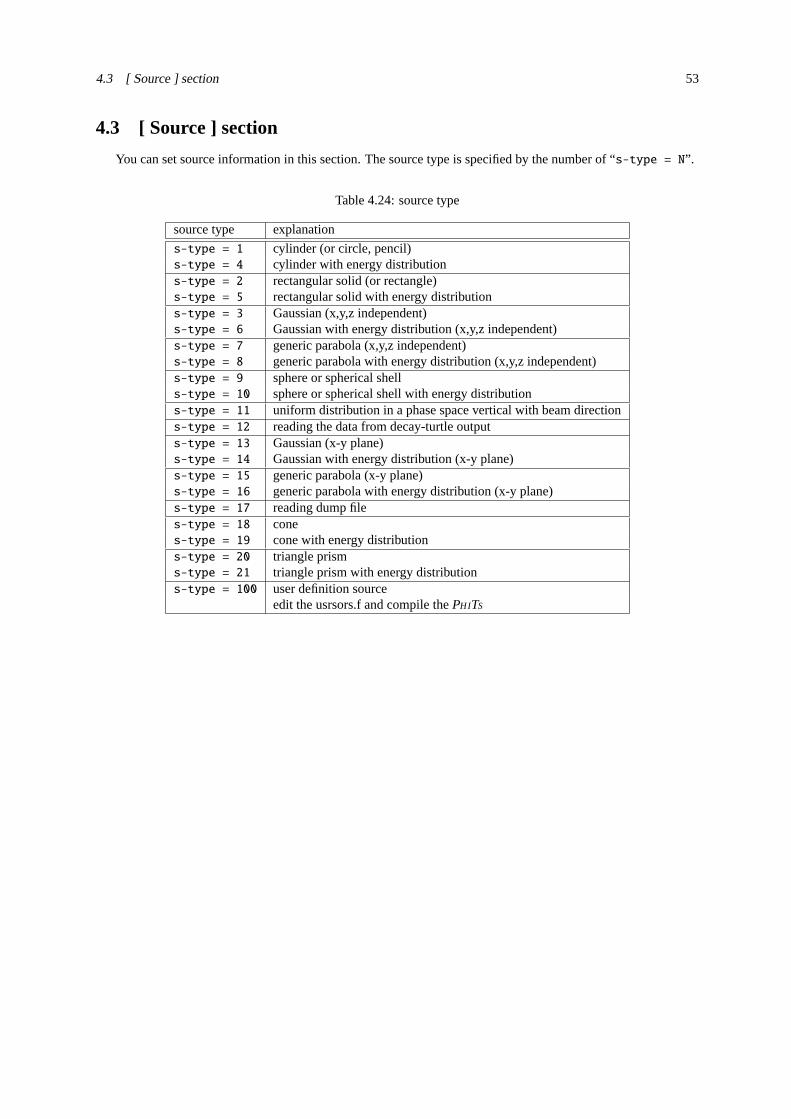
4.3 [ Source ] section 53
4.3 [ Source ] section
You can set source information in this section. The source type is specified by the number of “s-type = N”.
Table 4.24:source type
source type explanation
s-type = 1 cylinder (or circle, pencil)s-type = 4 cylinder with energy distributions-type = 2 rectangular solid (or rectangle)s-type = 5 rectangular solid with energy distributions-type = 3 Gaussian (x,y,z independent)s-type = 6 Gaussian with energy distribution (x,y,z independent)s-type = 7 generic parabola (x,y,z independent)s-type = 8 generic parabola with energy distribution (x,y,z independent)s-type = 9 sphere or spherical shells-type = 10 sphere or spherical shell with energy distributions-type = 11 uniform distribution in a phase space vertical with beam directions-type = 12 reading the data from decay-turtle outputs-type = 13 Gaussian (x-y plane)s-type = 14 Gaussian with energy distribution (x-y plane)s-type = 15 generic parabola (x-y plane)s-type = 16 generic parabola with energy distribution (x-y plane)s-type = 17 reading dump files-type = 18 cones-type = 19 cone with energy distributions-type = 20 triangle prisms-type = 21 triangle prism with energy distributions-type = 100 user definition source
edit the usrsors.f and compile thePHITS

54 4 SECTIONS FORMAT
4.3.1 <Source> : Multi-source
By this multi-source function, one can define plural sources specified bys-type. Each source begins<source>= number, which defines the relative weight of the multi-sources. Bytotfact = , a global normalization is de-fined. Note that you should not write<source> in the next line of the line wherereg parameter was written.
Table 4.25:multi-source
parameter explanation
<source> = defines a multi-source, the relative weight is defined by this numbertotfact = (D=1) global normalization factor
If this is given by a positive number, the source particle is generatedaccording to this ratio. If negative, the same particle is generated ineach multi-source section changing the weight according to the ratio.
iscorr = (D=0) Multi-source correlation option.0: Normal multi-source.1: Correlated multi-source. In this case, sources from each multi-sourcegroup are generated as an event. This option is useful for estimatingdetector response by nuclear reactions producing several secondaryparticles. Note that the locations of all sources generated in an event arenot the same, unlike in the case ofiscorr=2,3.2: Correlated multi-source. In this case, the locations of all sourcesgenerated in an event are the same. This mode is useful for simulating anuclear reaction occurred at arbitrary locations.3: Correlated multi-source. In this case, the locations of all sourcesgenerated in an event are the same, and the directions of second sourceis opposite to the first one. This mode is useful for simulating a particledecayed into 2 particles at arbitrary locations.
You have to specify the multiplicity of each source in an integer valueas its<source> parameter, and sum of the multiplicities as thetotfactparameter. For example, if you would like to simulate (X,1p2n) reactionas an event, you have to set<source> = 1 and 2 for proton and neutronsources, respectively, andtotfact = 3.

4.3 [ Source ] section 55
4.3.2 Common parameters
Common parameters for each source type are shown below. The order of the parameters in the source section isfree. If a parameter has a default value (D=***), the parameter can be omissible. The energy ofd, t, α and nucleusis specified by [MeV/nucleon].
Table 4.26:common source parameters 1
parameter explanation
proj = projectile : see Table3.4for specificationsx = (D=0) x-component of spinsy = (D=0) y-component of spinsz = (D=0) z-component of spinreg = (D=all) The source region can be restricted within overlaps between regions
defined by eachs-type and those specified by this parameter.The format is asreg = 1 - 5 10 34. You can use the lattice and universeframe asreg = ( 6 < 10[1 0 0] < u=3 ). See the section about tallyregion specification for details.
ntmax = (D=1000) maximum re-try number whenreg is specified.trcl = (D=none) transform number, or definition of transformwgt = (D=1.0) weight of source particlefactor = (D=1.0) Normalization factor of source particle.PHITS multiplies all results of
tally by factor. When you use multi-source, you should usetotfact insteadof factor. When you don’t use multi-source,totfact * factor is an actualnormalization factor.
izst = (D=charge of particle specified withproj=) Charge state of source particle.This has an effect only on a motion in the magnetic and electric fields definedin [magnetic field] and[electro magnetic field] sections.The charge number defined withizst doesn’t change while the particle moves.It should be noted that particles produced from nuclear reactions are not affectedby the value ofizst; the charge of the produced particle is given as its atomicnumber.
θ
z
xy
cosθ=dir
φ=phi
ψ=dom
Figure 4.2:Source direction and parame-tersdir, phi, dom.
A projectile direction is specified by 3 parameters:dir, phi,anddom. The relation between these is shown in Fig.4.2. The direc-tion is noted by a thick arrow. Thedir is a direction cosine againstthezaxis. Thephi is an azimuthal angle from thex axis in degree. Ifyou do not set it, a value of the azimuthal cosine is selected randomly.Using the parameterdom spreads out the direction determined bydirandphi by solid angle 2π(1−cosψ), whereψ = dom given in degree.In thePHITS calculation, the angle is given randomly within the solidangle.
When you setdir=all, the direction of the source beam becomesisotropic. If you want to use any angular distribution, a subsectionstarted froma-type is required, in which you should give the distri-bution by numerical data or analytic functions.
In s-type=9 and 10, the definition ofdir is different. Ins-type=11 and12, you can set onlydir= 1 or−1.
You can use the transform of coordinate bytrcl parameter whichspecify the transform number or the definition of transformation it-self. The relation ofwgt andfactor is reciprocal.
If the spin is not defined or zero, the neutron goes into the magnetic field without spin. In this case, the initialspin of neutron is determined at the entrance of the magnetic field by the direction of the magnetic field and thepolarization factor. If the spin is defined in this section, the neutron goes into the magnetic field with the spindirection irrespective of the direction of the magnetic field nor polarization.

56 4 SECTIONS FORMAT
Table 4.27:common source parameters 2
parameter explanation
ispfs = 0, 1, 2 (D=0) Spontaneous fission sourceIf ispfs = 1 or 2 is specified in[source] section and the following 18 nucleiare chosen asproj, one can define neutrons from spontaneous fission as a source.We assume these 18 nuclei as spontaneous fission nuclei,U-238, Pu-238, Pu-240, Pu-242, Cm-242, Cm-244, Cf-252, Th-232, U-232,U-233, U-234, U-235, U-236, Np-237, Pu-239, Pu-241, Am-241, Bk-249.ispfs = 1 : tally result is normalized by the number of spontaneous fissionsispfs = 2 : tally result is normalized by the number of neutrons produced byspontaneous fission.In the case ofispfs = 1,2, e0 ande-type, dir anda-type are neglected.
Whenispfs=1,2 is specified, the multiplicity of neutron and its energy spectrum are taken from the paper.25
The PHITS development team is grateful to Dr. Liem Peng Hong of NAIS, Co., Inc. for his support on developingthe function to generate the neutron sources.
In the next example, becauseproj=240Pu andispfs=1 are set, neutrons from spontaneous fission of Pu-240are used as source particles. In this case, the value ofe0 is invalid.
[ S o u r c e ]
s-type = 1
proj = 240Pu
e0 = 1.0
z0 = 0
z1 = 0
r0 = 0.0
dir = 1.0000
ispfs = 1
25 J. M. Verbeke, C. Hagmnn, and D. Wright, “Simulation of Neutron and Gamma Ray Emission from Fission and Photofission”, UCRL-AR-228518 (2014).

4.3 [ Source ] section 57
4.3.3 Cylinder distribution source
Parameters for cylinder source are shown below. The order of parameters is free. If a parameter has a defaultvalue (D=***), the parameter can be omissible.
Table 4.28:parameters for cylinder source
s-type = 1, 4 cylinder or circle sourcex0 = (D=0.0) x coordinate of center position of cylinder source (cm)y0 = (D=0.0) y coordinate of center position of cylinder source (cm)z0 = minimum z of cylinder source (cm)z1 = maximum z of cylinder source (cm), (when z1=z0, circle plane source)r0 = radius of cylinder source, (when r0=0.0, pencil source) (cm)r1 = (D=0.0) inner radius for inner void of cylinderdir = direction cosine of projectile against z axis
If you setall, it is isotropicIf you setdata, a-type subsection is necessary
phi = (D=none; random) azimuthal angle (degree)。
dom = (D=0.0) solid angle (degree)。= -1 ; cos2 bias distribution
e0 = projectile energy (s-type=1) (MeV)
4.3.4 Rectangular solid distribution source
Parameters for rectangular solid source are shown below. The order of parameters is free. If a parameter has adefault value (D=***), the parameter can be omissible.
Table 4.29:parameters for rectangular solid source
s-type = 2, 5 rectangular solid and rectangle sourcex0 = minimum x coordinate (cm)x1 = maximum x coordinate (cm)y0 = minimum y coordinate (cm)y1 = maximum y coordinate (cm)z0 = minimum z coordinate (cm)z1 = maximum y coordinate (cm), when (z1=z0), rectangle sourcedir = direction cosine from z axis
If you setall, isotropicIf you setdata, a-type subsection is necessary
phi = (D=none; random) azimuthal angle (degree)。
dom = (D=0.0) solid angle (degree)。= -1 ; cos2 bias distribution
e0 = projectile energy (s-type=2) (MeV)

58 4 SECTIONS FORMAT
4.3.5 Gaussian distribution source (x,y,z independent)
This Gauss distribution is consist of independent Gaussian in each x, y, z direction. Parameters for Gaussiansource are shown below. The order of parameters is free. If a parameter has a default value (D=***), the parametercan be omissible.
Table 4.30:parameters for Gaussian source
s-type = 3, 6 Gaussian sourcex0 = (D=0.0) x coordinate of Gaussian center (cm)x1 = FWHM in x direction (cm)y0 = (D=0.0) y coordinate of Gaussian center (cm)y1 = FWHM in y direction (cm)z0 = (D=0.0) z coordinate of Gaussian center (cm)z1 = FWHM in z direction (cm)dir = direction cosine from z axis
If you setall, isotropicIf you setdata, a-type subsection is necessary
phi = (D=none; random) azimuthal angle (degree)。
dom = (D=0.0) solid angle (degree)。= -1 ; cos2 bias distribution
e0 = projectile energy(s-type=3) (MeV)
4.3.6 Generic parabola distribution source (x,y,z independent)
This generic parabola distribution is consist of independent parabola in each x, y, z direction. Parameters forgeneric parabola source are shown below. The order of parameters is free. If a parameter has a default value(D=***), the parameter can be omissible.
Table 4.31:parameters for generic parabola distribution
s-type = 7, 8 generic parabola sourcex0 = (D=0.0) x coordinate of X-parabola center (cm)x1 = X-parabola width(cm)y0 = (D=0.0) y coordinate of Y-parabola center (cm)y1 = Y-parabola width(cm)z0 = minimum z of parabola (cm)z1 = maximum z of parabola (cm)rn = (D=2) order of generic paraboladir = direction cosine from z axis
If you setall, isotropicIf you setdata, a-type subsection is necessary
phi = (D=none; random) azimuthal angle (degree)。
dom = (D=0.0) solid angle (degree)。= -1 ; cos2 bias distribution
e0 = projectile energy (s-type=7) (MeV)

4.3 [ Source ] section 59
4.3.7 Gaussian distribution source (x-y plane)
This source is a Gaussian distribution in x-y plane. Parameters for Gaussian source are shown below. Theorder of parameters is free. If a parameter has a default value (D=***), the parameter can be omissible.
Table 4.32:parameters for Gaussian source
s-type = 13, 16 Gaussian sourcex0 = (D=0.0) x coordinate of Gaussian center (cm)y0 = (D=0.0) y coordinate of Gaussian center (cm)r1 = FWHM in x-y plane (cm)z0 = minimum z coordinate (cm)z1 = (D=z0) maximum z coordinate (cm)dir = direction cosine from z axis
If you setall, isotropicIf you setdata, a-type subsection is necessary
phi = (D=none; random) azimuthal angle (degree)dom = (D=0.0) solid angle (degree)
= -1 ; cos2 bias distributione0 = projectile energy(s-type=13) (MeV)
4.3.8 Generic parabola distribution source (x-y plane)
This source is a generic parabola distribution in x-y plane. Parameters for generic parabola source are shownbelow. The order of parameters is free. If a parameter has a default value (D=***), the parameter can be omissible.
Table 4.33:parameters for generic parabola distribution
s-type = 15, 16 generic parabola sourcex0 = (D=0.0) x coordinate of X-parabola center (cm)y0 = (D=0.0) y coordinate of Y-parabola center (cm)r1 = parabola width in x-y plane (cm)z0 = minimum z of parabola (cm)z1 = maximum z of parabola (cm)rn = (D=2) order of generic paraboladir = direction cosine from z axis
If you setall, isotropicIf you setdata, a-type subsection is necessary
phi = (D=none; random) azimuthal angle (degree)。
dom = (D=0.0) solid angle (degree)。= -1 ; cos2 bias distribution
e0 = projectile energy (s-type=15) (MeV)

60 4 SECTIONS FORMAT
4.3.9 Sphere and spherical shell distribution source
Parameters for sphere and spherical shell source are shown below. The order of parameters is free. If aparameter has a default value (D=***), the parameter can be omissible.
Table 4.34:parameters for sphere and spherical shell source
s-type = 9, 10 sphere and spherical shell sourcex0 = (D=0.0) x coordinate of sphere center (cm)y0 = (D=0.0) y coordinate of sphere center (cm)z0 = (D=0.0) z coordinate of sphere center (cm)r1 = inside radius (cm). If r1=0, sphere sourcer2 = outside radius (cm)dir = direction
dir = 1.0 : outgoing from the center with normal line directiondir = -1.0 : inverse direction with dir=1.0dir = all : isotropicdir = -all : inverse direction against dir=1.0, and with cosine distribution.This is used for volume and area calculation with cos2 biasdir = iso : uniform distribution on a circle of radiusr2 on a sphericalshell of radiusr1 with the direction orthogonal to the circle ofr2 towardthe sphere. In the case ofr1=r2, the result is almost the same asdir = -all, but an effect of the weight on it is not included. Therefore,using the condition, you can obtain the variance of deposition energies onthe[t-deposit] tally with output = deposit.
e0 = projectile energy (s-type=9) (MeV)
When you use the source type s-type=9 for volume and area calculation, you should set asdir = -all, r1= r2 . And,dir = iso also gives the same result.
r2
r1
Figure 4.3: Schematic image of the source in the case ofdir=iso.

4.3 [ Source ] section 61
4.3.10 s-type= 11
This is a uniform distribution source in a phase space which is vertical with beam direction. Parameters forthis source type are shown below. The order of parameters is free. If a parameter has a default value (D=***), theparameter can be omissible.
Table 4.35:parameters for s-type= 11
s-type = 11 uniform distribution in a phase space vertical with beam directionx0 = (D=0.0) x coordinate of beam center (cm)x1 = ratio of (maximum radius)/(minimum radius) for x direction (cm/mrad)y0 = (D=0.0) y coordinate of beam center (cm)y1 = ratio of (maximum radius)/(minimum radius) for y direction (cm/mrad)z0 = minimum z (cm)z1 = maximum z (cm)rx = gradient of ellipse in a phase space on x direction (rad)ry = gradient of ellipse in a phase space on y direction (rad)wem = emittance (π cm× mrad )dir = direct cosine (1 or -1 only)e0 = projectile energy (MeV)
4.3.11 s-type= 12
In this source type, decay-turtle output is read as source. Parameters for this source type are shown below. Theorder of parameters is free. If a parameter has a default value (D=***), the parameter can be omissible.
The input file is rewinded and re-used from the first particle again, if all of source in decay-turtle is read beforethe calculation finishes.
Table 4.36:parameters for s-type= 12
s-type = 12 decay-turtle readingx0 = (D=0.0) x coordinate offset of beam (cm)y0 = (D=0.0) y coordinate offset of beam (cm)z0 = (D=0.0) z coordinate offset of beam (cm)dir = direction cosine(1 or -1 only)file = decay-turtle filename (with full pathname)
The format ofdecay-turtle is double precision, and ascii, and each record is as
xp, xq, yp, yq, e0, wt0, pz0
Table 4.37:decay-turtle data
variable explanation
xp, yp incoming position of beam particle (cm)xq, yq angle against vertical face with beam direction (mrad)e0 momentum of beam particle (GeV/c)wt0 weight of beam particlepz0 polarizing of beam particle (be not in use)

62 4 SECTIONS FORMAT
4.3.12 Cone shape
Parameters for cone shape source are shown below. The order of parameters is free. If a parameter has a defaultvalue (D=***), the parameter can be omissible.
Table 4.38:parameters for cone shape
s-type = 18, 19 Cone shapex0 = (D=0.0) x coordinate offset of top of cone (cm)y0 = (D=0.0) y coordinate offset of top of cone (cm)z0 = (D=0.0) z coordinate offset of top of cone (cm)x1 = x-component of vector from top to center of bottom circle (cm)y1 = y-component of vector from top to center of bottom circle (cm)z1 = z-component of vector from top to center of bottom circle (cm)r0 = (D=0.0) distance between top and upper end of source
locations on axis of cone (cm)r1 = distance between top and lower end of source
locations on axis of cone (cm)r2 = angle between generatrix and axis of cone (degree)dir = direction cosine from z axis
If you setall, isotropicIf you setdata, a-type subsection is necessary
phi = (D=none; random) azimuthal angle (degree)。
dom = (D=0.0) solid angle (degree)。= -1 ; cos2 bias distribution
e0 = projectile energy (s-type=18) (MeV/u)

4.3 [ Source ] section 63
4.3.13 Triangle prism shape
Parameters for triangle prism shape source are shown below. The order of parameters is free. If a parameterhas a default value (D=***), the parameter can be omissible.
Table 4.39:parameters for triangle prism shape
s-type = 20, 21 Triangle prism shapex0 = (D=0.0) x-coordinate of origin apex of triangle (cm)y0 = (D=0.0) y-coordinate of origin apex of triangle (cm)z0 = (D=0.0) z-coordinate of origin apex of triangle (cm)x1 = x vector from the origin to the first apex (cm)y1 = y vector from the origin to the first apex (cm)z1 = z vector from the origin to the first apex (cm)x2 = x vector from the origin to the second apex (cm)y2 = y vector from the origin to the second apex (cm)z2 = z vector from the origin to the second apex (cm)x3 = x vector from the origin to the third apex (cm)y3 = y vector from the origin to the third apex (cm)z3 = z vector from the origin to the third apex (cm)exa = attenuation coefficient. exa>0; exp (−ax), exa=0; uniformdir = direction cosine from z axis
If you setall, isotropicIf you setdata, a-type subsection is necessary
phi = (D=none; random) azimuthal angle (degree)。
dom = (D=0.0) solid angle (degree)。= -1 ; cos2 bias distribution
e0 = projectile energy (s-type=20) (MeV/u)
Figure 4.4:Coordinates of triangle prism

64 4 SECTIONS FORMAT
4.3.14 Reading dump file
When you settype = 17, you can use information on particles recorded in a file as sources. The “dump ”filecan be obtained by using the dump option in the[t-cross], [t-product], and[t-time] tallies. There aretwo ways to treat the dump data, which can be switched by theidmpmode parameter. Each particle data recorded inthe dump file was treated as an independent history withidmpmode=0. On the other hand, using history informationrecorded in the dump file, the correlations between particles at the time of data dump are taken into account in thestatistical processing withidmpmode=1. For the continuous calculation using dump file, we recommend to useidmpmode=1 by taking account of the history information at the previous step.26
Parameters for thetype = 17 are shown below. The order of parameters is free. If a parameter has a defaultvalue (D=***), the parameter can be omissible.
Table 4.40:parameters for dump file source(1)
s-type = 17 reading dump filefile = dump filename (with full pathname)dump = number of dump data. if it is negative, data is written by Ascii.
(next line) identification of dump data(omissible) If below parameters are specified, these values have priority
over the dump data. If the dump data does not include the following data,one should specify the parameters.
x0 = minimum x coordinate (cm)x1 = maximum x coordinate (cm)y0 = minimum y coordinate (cm)y1 = maximum y coordinate (cm)z0 = minimum z coordinate (cm)z1 = maximum z coordinate (cm)sx = (D=0) x-component of spinsy = (D=0) y-component of spinsz = (D=0) z-component of spindir = direction cosine from z axis
If you setall, isotropicIf you setdata, a-type subsection is necessary
phi = (D=none; random) azimuthal angle (degree)dom = (D=0.0) solid angle (degree)
= -1 ; cos2 bias distributione0 = projectile energy (MeV)
e-type = type of energy distributionwgt = (D=1.0) weight of source particle
26 The optionidmpmode=1 and re-used calculation using the optiondmpmulti were introduced by referring to the presentation “Estimationof uncertainty in multi-step Monte Carlo calculation”(N50) by Dr. Y. Namitoet al. at the 2015 annual meeting of AESJ (Hitachi, Japan).

4.3 [ Source ] section 65
Table 4.41:parameters for dump file source(2)
(omissible) one can also specify below parametersfactor = (D=1.0) normalization of source particlet-type = (D=0) time distributionreg = (D=all) specify the regionntmax = (D=1000) maximum re-try number whenreg is specifiedtrcl = (D=none) transform number, or definition of transform
idmpmode = Control parameter to select dump source mode.(D=0) In case history information (nocas and nobach) is not included in the dump data.(D=1) In case history information (nocas and nobach) is included in the dump data.=0: Each particle data recorded in the dump file is treated as an independent history.=1: Particle data in the dump file are processed by taking account of particle correlationsin the previous step.
dmpmulti = Control parameter for reuse of dump file.(D=0.0) withidmpmode=0(D=1.0) withidmpmode=1=0.0: The dump file is rewinded and re-used until finishing total histories specifiedby (maxcas*maxbch). However, this mode cannot be used withidmpmode=1.>0.0: The dump file is re-used in the number of times specified by this parameter.The digits after the decimal point are reflected to the probability in the Russian rouletteto adopt another reproduction of the particle data.
The history number (nocas) and the batch number (nobch) must be contained in the dump data to useidmpmode=1.Using the dump option of PHITS tally, a dump file named “***dmp” is created as well as the normal tally filewith the file name “***” specified by “file=***”. Both files are required to useidmpmode=1 and needed to beplaced in the same folder. The total number of histories of the previous step is adopted from the values ofmaxcas
andmaxbch written in this tally file and the history numbers,maxcas andmaxbch, given in the PHITS input fileare neglected. The normalization factortotfact is ignored withidmpmode=1. To use the normalization factor,totfact should be applied to the previous step for creating the dump file, and then, it will be reflected in theweights of particles recorded in the dump file. The optionidmpmode=1 is incompatible with multi-source.
The optiondmpmulti controls the number of re-use of the dump file. In the case ofdmpmulti=2.0, the dumpfile will be reused twice. Namely, information for each particle recorded in the dump file is reproduced twice andthey are treated as two particles having a half weight with a different random number. The digits after the decimalpoint indicate the probability to create another reproduction of the particle. The reproduction is stochasticallydetermined by the Russian roulette for each particle. For example, in case ofdmpmulti=2.3, the particle dataare reproduced twice with the probability 70% and three times with the probability 30%. As a special mode withdmpmulti=0.0, the dump file is rewinded and re-used until finishing total histories specified by (maxcas*maxbch)written in the PHITS input file. This mode is valid only withidmpmode=0.
Basically, the restart calculation (istdev<0) is not applicable for the dump source calculation. It is onlyallowed withdmpmulti=0.0, but then it should be noticed that the calculation may give biased results unlessthe dump file contains large enough particle data. Therefore, re-calculation taking largerdmpmulti factor ismore recommended to achieve better statistics. If the particle data contained in the dump file are not statisticallysufficient, statistical errors may not become small as aimed even though taking a largedmpmulti factor. In thiscase, re-calculation from the previous step to create sufficient dump data is required.
By the parameter of “dump =”, the number of the dump data in one record is specified. If this number is givenby positive number, the data is read as binary data. If negative, the data is read as asci data. In next line, the datasequence of one record is described. The relation between the physical quantities and id number is the followings,
Table 4.42:id number of dump data (1)
physical quantities kf x y z u v w e wt time c1 c2 c3 sx sy szid number 1 2 3 4 5 6 7 8 9 10 11 12 13 14 15 16

66 4 SECTIONS FORMAT
Table 4.43:id number of dump data (2)
physical quantities name nocas nobch noid number 17 18 19 20
Here kf means the kf-code of the particles (see Table3.4), x, y, z are coordinates (cm), u, v, w denote the unitvectors of the direction of the particle, e is the energy (MeV, or MeV/nucleon for nucleus), wt is the weight, timeis the initial time (ns), c1, c2, c3 are the values of counters, and sx, sy, sz are the unit vectors of the direction ofspin, respectively. name is a collision number of the particle, nocas is a history number of a batch, nobch is abatch number, no is a cascade id in the history. These are assumed as real*8 for the binary data,n(1p1e24.15) dataformat for the ascii data.
For an example, one record has 9 data as
kf e wt x y z u v w
To read this data, we write the parameters as
dump = 9
1 8 9 2 3 4 5 6 7

4.3 [ Source ] section 67
4.3.15 User definition source
If you edit usrsors.f, you can use your original source function by s-type=100. If the following parameters areset, these values have the priority. If a parameter has a default value (D=***), the parameter can be omissible.
Table 4.44:the parameters can be specified in s-type=100
s-type = 100 user definition sourceIf below parameters are specified, these values have priorityover the user defined data.
x0 = minimum x coordinate (cm)x1 = maximum x coordinate (cm)y0 = minimum y coordinate (cm)y1 = maximum y coordinate (cm)z0 = minimum z coordinate (cm)z1 = maximum z coordinate (cm)sx = (D=0) x-component of spinsy = (D=0) y-component of spinsz = (D=0) z-component of spindir = direction cosine from z axis
If you setall, isotropicIf you setdata, a-type subsection is necessary
phi = (D=none; random) azimuthal angle (degree)。
dom = (D=0.0) solid angle (degree)。= -1 ; cos2 bias distribution
e0 = projectile energy (s-type=7) (MeV)e-type = type of energy distributionwgt = (D=1.0) weight of source particlefactor = (D=1.0) normalization of source particlet-type = (D=0) time distributionreg = (D=all) specify the regionntmax = (D=1000) maximum re-try number whenreg is specified.trcl = (D=none) transform number, or definition of transform

68 4 SECTIONS FORMAT
We show a sample program of usrsors.f as following. In the first comment part, there is a list of the variableswhich is necessary to define the source. Next there is a list of kf-code which specifies the source particle. In thelast part of the comment, the random number functions, one is an uniform random number, the other is a Gaussianrandom number, are shown. The first part of the program is an example of the initialization, which describes theopen and close the data file. The remaining part shows a list of the variables which user should define in thissubroutine.
List 4.1• usrsors.f
1: ************************************************************************
2: subroutine usrsors(x,y,z,u,v,w,e,wt,time,name,kf,nc1,nc2,nc3,
3: & sx,sy,sz)
4: * sample subroutine for user defined source. *
5: * variables : *
6: * x, y, z : position of the source. *
7: * u, v, w : unit vector of the particle direction. *
8: * e : kinetic energy of particle (MeV). *
9: * wt : weight of particle. *
10: * time : initial time of particle. (ns) *
11: * name : usually = 1, for Coulmb spread. *
12: * kf : kf code of the particle. *
13: * nc1 : initial value of counter 1 *
14: * nc2 : initial value of counter 2 *
15: * nc3 : initial value of counter 3 *
16: * sx,sy,sz : spin components *
17: *----------------------------------------------------------------------*
18: * kf code table *
19: * kf-code: ityp : description *
20: * 2212 : 1 : proton *
21: * 2112 : 2 : neutron *
22: * 211 : 3 : pion (+) *
23: * 111 : 4 : pion (0) *
24: * -211 : 5 : pion (-) *
25: * -13 : 6 : muon (+) *
26: * 13 : 7 : muon (-) *
27: * 321 : 8 : kaon (+) *
28: * 311 : 9 : kaon (0) *
29: * -321 : 10 : kaon (-) *
30: * kf-code of the other transport particles *
31: * 12 : nu_e *
32: * 14 : nu_mu *
33: * 221 : eta *
34: * 331 : eta’ *
35: * -311 : k0bar *
36: * -2112 : nbar *
37: * -2212 : pbar *
38: * 3122 : Lanbda0 *
39: * 3222 : Sigma+ *
40: * 3212 : Sigma0 *
41: * 3112 : Sigma- *
42: * 3322 : Xi0 *
43: * 3312 : Xi- *
44: * 3334 : Omega- *
45: *----------------------------------------------------------------------*
46: * available function for random number *
47: * unirn(dummy) : uniform random number from 0 to 1 *
48: * gaurn(dummy) : gaussian random number *
49: * for exp( - x**2 / 2 / sig**2 ) : sig = 1.0 *
50: ************************************************************************
51: implicit real*8 (a-h,o-z)
52: *-----------------------------------------------------------------------
53: parameter ( pi = 3.141592653589793d0 )

4.3 [ Source ] section 69
54: data ifirst / 0 /
55: save ifirst
56: character filenm*50
57: *-----------------------------------------------------------------------
58: * example of initialization
59: *-----------------------------------------------------------------------
60: if( ifirst .eq. 0 ) then
61: c filenm = ’input.dat’
62: c inquire( file = filenm, exist = exex )
63: c if( exex .eqv. .false. ) then
64: c write(*,*) ’file does not exist => ’, filenm
65: c call parastop( 887 )
66: c end if
67: c open(71, file = file(i), status = ’old’ )
68:
69: c close(71)
70: ifirst = 1
71: end if
72: *-----------------------------------------------------------------------
73: * example for 3 GeV proton with z-direction
74: *-----------------------------------------------------------------------
75: x = 0.0
76: y = 0.0
77: z = 0.0
78: u = 0.0
79: v = 0.0
80: w = 1.0
81: e = 3000.0
82: wt = 1.0
83: time = 0.0
84: name = 1
85: kf = 2212
86: nc1 = 0
87: nc2 = 0
88: nc3 = 0
89: sx = 0.d0
90: sy = 0.d0
91: sz = 0.d0
92: *-----------------------------------------------------------------------
93: return
94: end

70 4 SECTIONS FORMAT
4.3.16 Definition for energy distribution
In the energy distributed source types-type = 4, 5, 6, 8, 10, 14, and16, ors-type = 17, 100 with e-typeparameter, energy distribution parameters are required as shown below. Ford, t, α and nucleus, this energy isexpressed in units of [MeV/nucleon].
For e-type = 1,4,11,14, the source intensity in each energy bin should be given in the energy integratedvalue. Fore-type = 21,24,31,34, you should give the source intensity in each energy bin as the energy differ-ential value expressed in [particles/MeV]. For e-type = 2,3,5,6,7,12,14,15,16, you can define the energydifferential spectrum using various functions. Fore-type = 8,9,18,19, you can define the source intensitydiscretely. Fore-type = 28,29, you can use the RI-source function.
If a parameter has a default value (D=***), the parameter can be omissible.
Table 4.45:parameters for source energy distribution (1)
parameter explanation
e-type = 1, (11) You can specify any energy distribution by giving data set of energy binse(i)
and integrated values of the particle generation probabilityw(i) by hand.The number of the particle generation in the bin is proportional tow(i), andthe specified energy distribution is statistically described.For 11 case, energy is given by wave length (Å).
ne = Number of energy group.If it is given by positive number, source particles are generated so that theenergy differential fluxes in the unit of [1/MeV] become constant in eachbin. On the other hand, ifne is negative, the fluxes in the unit of [1/Lethargy]become constant in each bin.Data must be given from the next line by the format as(e(i),w(i),i=1,ne), e(ne+1).The integrated number of the particle generation in the each energy binis proportional tow(i).
e-type = 4, (14) You can specify the same energy distribution as is the case ofe-type = 1, (11). Unlike e-type = 1, (11), the distributionis described by giving data set of energy binse(i) and weightsof the source particlew(i) by hand. The number of sourceparticles generated in each bin is the same for all energy bin,but integrated values of the weight of source particles are adjustedto be proportional tow(i).You can also change the number of source particles generated in each binby specifingp(i).For 14 case, energy is given by wave length (Å).
ne = Number of energy group.If it is given by positive number, source particles are generated so that theenergy differential fluxes in the unit of [1/MeV] become constant in eachbin. On the other hand, ifne is negative, the fluxes in the unit of [1/Lethargy]become constant in each bin.Data must be given from the next line by the format as(e(i),w(i),i=1,ne), e(ne+1).In default (p-type=0), equal number of particle is generated in each cell.The integrated number of source particles generated in each binis proportional top(i).
p-type = 0, 1 (D=0) generation optionfor 0, p(i)=1 for all i is assumed without the following datafor 1, p(i) must be given from the next line by the format as(p(i),i=1,ne)
For neutron optics, we prepare an alternative option to specify the energy as wave length. If you specify e-type=11, 12, 14, you can use wave length (Å) as an energy unit. For the other case, you can use the mathematicalexpressions as e0=8.180425e-8/13**2, which gives the energy of neutron with 13Åwave length.

4.3 [ Source ] section 71
In the case ofe-type = 1, the format is as follows.
e-type = 1
ne = n
e(1) w(1)
e(2) w(2)
e(3) w(3)
.... ...
e(n-1) w(n-1)
e(n) w(n)
e(n+1)
In this case, the energy distribution is given as,
e(1)-e(2) w(1)
e(2)-e(3) w(2)
e(3)-e(4) w(3)
....... ...
e(n-1)-e(n) w(n-1)
e(n)-e(n+1) w(n)
If you want to set the strength of three energy bins between 0-2MeV, 2-4MeV, and 4-6MeV to be 0.2, 0.6, and 0.2,respectively, an example is as follows.
e-type = 1
ne = 3
0 0.2
2 0.6
4 0.2
6

72 4 SECTIONS FORMAT
Table 4.46:parameters for source energy distribution (2)
parameter explanation
e-type = 21, (31) You can specify any energy distribution by giving data set of energy binse(i)
and differential probabilities of the particle generationdφ/dE(i) by hand.The integrated number of the particle generation in the bin is proportional todφ/dE(i)*e(i+1)-e(i), and the specified energy distributionis statistically described.For 31 case, energy is given by wave length (Å).
ne = Number of energy group.If it is given by positive number, source particles are generated so that theenergy differential fluxes in the unit of [1/MeV] become constant in eachbin. On the other hand, ifne is negative, the fluxes in the unit of [1/Lethargy]become constant in each bin.Data must be given from the next line by the format as(e(i),dφ/dE(i),i=1,ne), e(ne+1).The integrated number of the particle generation in the each energy binis proportional todφ/dE(i)*e(i+1)-e(i).
e-type = 24, (34) You can specify the same energy distribution as is the case ofe-type = 21, (31). Unlike e-type = 21, (31), the distributionis described by giving data set of energy binse(i) and weightsof the source particlew(i) by hand. The number of sourceparticles generated in each bin is the same for all energy bin,but integrated values of the weight of source particles are adjustedto be proportional tow(i)*e(i+1)-e(i).You can also change the number of source particles generated in each binby specifingp(i).For 34 case, energy is given by wave length (Å).
ne = Number of energy group.If it is given by positive number, source particles are generated so that theenergy differential fluxes in the unit of [1/MeV] become constant in eachbin. On the other hand, ifne is negative, the fluxes in the unit of [1/Lethargy]become constant in each bin.Data must be given from the next line by the format as(e(i),w(i),i=1,ne), e(ne+1).In default (p-type=0), equal number of particle is generated in each cell.The integrated number of source particles generated in each binis proportional top(i).
p-type = 0, 1 (D=0) generation optionfor 0, p(i)=1 for all i is assumed without the following datafor 1, p(i) must be given from the next line by the format as(p(i),i=1,ne)

4.3 [ Source ] section 73
Table 4.47:parameters for source energy distribution (3)
parameter explanation
e-type = 8, (18) You can specify any energy distribution by giving data set of energy pointse(i)
and probabilities of the particle generationw(i) by hand.The number of the particle generation at the point is proportional tow(i), andthe specified energy distribution is statistically described.For 18 case, energy is given by wave length (Å).
ne = Number of energy points.Data must be given from the next line by the format as(e(i),w(i),i=1,ne).The number of the particle generation at the each energy point is proportionalto w(i).
e-type = 9, (19) You can specify the same energy distribution as is the case ofe-type = 8, (18). Unlike e-type = 8, (18), the distributionis described by giving data set of energy pointse(i) and weightsof the source particlew(i) by hand. The number of sourceparticles generated in each point is the same for all energy point,but integrated values of the weight of source particles are adjustedto be proportional tow(i).You can also change the number of source particles generated in each pointby specifingp(i).For 19 case, energy is given by wave length (Å).
ne = Number of energy points.Data must be given from the next line by the format below.In default (p-type=0), equal number of particle is generated at each point.(e(i),w(i),i=1,ne)
The number of source particles generated in each pointis proportional top(i).
p-type = 0, 1 (D=0) generation optionfor 0, p(i)=1 for all i is assumed without the following datafor 1, p(i) must be given from the next line by the format as(p(i),i=1,ne)

74 4 SECTIONS FORMAT
Table 4.48:parameters for source energy distribution (4)
parameter explanation
e-type = 2, (12) Differential spectrumdφ/dE(i) is given by Gaussian distribution.For 12 case, energy is given by wave length (Å).
eg0 = center of Gaussian distribution (MeV)eg1 = FWHM of Gaussian distribution (MeV)eg2 = minimum cut off for Gaussian distribution (MeV)eg3 = maximum cut off for Gaussian distribution (MeV)
e-type = 3 Differential spectrumdφ/dE(i) is given by Maxwellian distribution:f (x) = x1.5 exp(−x/T)
nm = (D=-200) number of energy groupIf it is given by positive number, linear interpolation is assumed in a bin.If negative, logarithmic interpolation is assumed in a bin.
et0 = temperature parameter T (MeV)et1 = minimum cut off for Maxwellian distribution (MeV)et2 = maximum cut off for Maxwellian distribution (MeV)
e-type = 7 You can specify the same energy distribution as is the case ofe-type = 3. Unlike e-type = 3, the number of source particlesgenerated in each bin is the same for all energy bin, but integrated valuesof the weight of source particles are adjusted to be proportionalto f (x) = x1.5 exp(−x/T).You can also change the number of source particles generated in each binby specifingp(i).
nm = (D=-200) Number of energy group.If it is given by positive number, linear interpolation is assumed in a bin.If negative, logarithmic interpolation is assumed in a bin.In default (p-type=0), equal number of particle is generated in each cell.The integrated number of source particles generated in each binis proportional top(i).
et0 = temperature parameter T (MeV)et1 = minimum cut off for Maxwellian distribution (MeV)et2 = maximum cut off for Maxwellian distribution (MeV)
p-type = 0, 1 (D=0) generation optionfor 0, p(i)=1 for all i is assumed without the following datafor 1, p(i) must be given from the next line by the format as(p(i),i=1,ne)

4.3 [ Source ] section 75
Table 4.49:parameters for source energy distribution (5)
parameter explanation
e-type = 5, (15) Differential spectrumdφ/dE(i) is given by f(x).For 15 case, energy is given by wave length (Å).
f(x) = Any analytical function of x, Fortran style.x denotes energy (MeV/u). One can use intrinsic functions and constants C.e.g.f(x) = exp(-c1*x**2)
nm = number of energy groupIf it is given by positive number, linear interpolation is assumed in a bin.If negative, logarithmic interpolation is assumed in a bin.Integrated number of source particles generated in each cell is proportional tof(x)
eg1 = minimum cut off for energy distribution (MeV)eg2 = maximum cut off for energy distribution (MeV)
e-type = 6, (16) You can specify the same energy distribution as is the case ofe-type = 5, (15). Unlike e-type = 5, (15), the number of sourceparticle generated in each bin is the same for all energy bin, butintegrated values of the weight of source particles are adjusted to beproportional tof (x).You can also change the number of source particles generated in each binby specifingp(i).For 16 case, energy is given by wave length (Å).
f(x) = Any analytical function of x, Fortran style.x denotes energy (MeV/u). One can use intrinsic functions and constants C.e.g.f(x) = exp(-c1*x**2)
nm = number of energy groupIf it is given by positive number, linear interpolation is assumed in a bin.If negative, logarithmic interpolation is assumed in a bin.In default (p-type=0), equal number of particle is generated in each cell.The integrated number of source particles generated in each binis proportional top(i).
eg1 = minimum cut off for energy distribution (MeV)eg2 = maximum cut off for energy distribution (MeV)
p-type = 0, 1 (D=0) generation optionfor 0, p(i)=1 for all i is assumed without the following datafor 1, p(i) must be given from the next line by the format as(p(i),i=1,nm)

76 4 SECTIONS FORMAT
Table 4.50:parameters for source energy distribution (6)
parameter explanation
e-type= 28,29 Photon sources with energy spectra of radioisotope (RI) decay are generated by simplyspecifying the activity (in Bq) and name of the RIs. Nuclear decay database DECDC27
is used to obtain the photon spectra. The database is equivalent to ICRP107. When youuse this function, you have to specify directory containing the DECDC data fileRIsource.dat by settingfile(24) (D=c:\phits\data\) in [parameters] section.Whene-type= 28, photon spectrum is expressed by changing the probability ofgenerating particle energy spectra obtained from DECDC.Whene-type= 29, photon spectrum is expressed by changing the weight of sourceparticles, while keeping the constant probability for all gamma-ray energy.
ni= Number of RIs. Name of the RIs and the activity must be given from the next line by theformat as(RI(i),A(i),i=1,ni).RI(i) can be defined by the format as 137Cs or Cs-137.A(i) is specified by the unit of Bq.
dtime= (D=−10.0) Option for time evolution (sec)dtime>0 (in sec): Photon spectrum is determined after considering the decay of thespecified RIs including the contributions from their daughter nuclides at the time whendtime has passed. The activity of each RI changed from its specified value. For example,when you set 100 Bq for a RI with half life of 1 min anddtime=60, the activity of the RIassumed in the PHITS calculation is 50 Bq.dtime=0: No time evolution is considered.dtime<0: Photon spectrum is determined after considering the decay of the specified RIsincluding the contributions from their daughter nuclides at the time when half-life×|dtime|has passed. Unlikedtime>0, the activity of each RI is not changed from its specifiedvalue. For example, when you set 100 Bq for a RI with half-life of 1 min anddtime=−1.0,the activity of the RI assumed in the PHITS calculation is still 100 Bq. When you haveno information on the time necessary to attain the radioactive equilibrium, you have toset a large negative value e.g.dtime=−10.0. You cannot specify both parent and daughternuclides at once fordtime<0.
When you use this function with multi-sources, you should set<source>=1.0 andtotfact as shown below.
• Settotfact to be the number of<source>, when all sources are defined bye-type = 28,29.
• Set each<source> to be absolute intensity of each RI and settotfact to be the sum of all values of<source>, when the multi-sources include sources defined bye-type,28,29.
27 A. Endo, Y. Yamaguchi and K.F. Eckerman, Nuclear decay data for dosimetry calculation - Revised data of ICRP Publication 38, JAERI1347 (2005).

4.3 [ Source ] section 77
Table 4.51:parameters for source energy distribution (7)
parameter explanation
(continued in the cases ofe-type= 28,29)actlow= (D=1.0e-10) Option for lower limit of the activity (Bq).
When the activity at the time the specified time has passed is smaller thanactlow, the gammadecay of its RI is not included in the photon sources.
norm= (D=0) Option for normalization of tally results.0: Tally results are normalized to the unit of (/sec). In this case, the source intensity is determinedby the specified activity. (Ifdtime>0, its decrease by the decay is also taken into account.)1: Tally results are normalized to the unit of (/source). This is equivalent to the generalnormalization of PHITS.
An example usinge-type = 28,29 is as follows.
[ S o u r c e ]
totfact = 2.0
<source> = 1.0
s-type = 4
proj = photon
dir = all
r0 = 0.
z0 = 0.
z1 = 0.
e-type = 28
ni = 1
Cs-137 100.
dtime = -10.0
actlow = 1.0
<source> = 1.0
s-type = 4
proj = photon
dir = all
r0 = 0.
z0 = 0.
z1 = 0.
e-type = 28
ni = 1
Cs-134 100.
dtime = -10.0
actlow = 1.0
In this case, the activity after the radioactive equilibrium of Cs-137 and Cs-134 of 100Bq each is defined asphoton sources. Furthermore, by settingactlow=1, the activity smaller than 1Bq is ignored.

78 4 SECTIONS FORMAT
4.3.17 Definition for angular distribution
If you setdir = data, angular distribution parameters are required as shown below. If a parameter has adefault value (D=***), the parameter can be omissible.
Table 4.52:parameters for source angular distribution (1)
parameter explanation
a-type = 1, (11) You can specify any angular distribution by giving data set of angle binsa(i)
and integrated values of the particle generation probabilityw(i) by hand.The number of the particle generation in the bin is proportional tow(i), andthe specified angular distribution is statistically described.For 1 case, angle is given by cosine, for 11 case, given by degree
na = Number of angular group.Data must be given from the next line by the format as(a(i),w(i),i=1,na), a(na+1).
a-type = 4, (14) You can specify the same angular distribution as is the case ofa-type = 1, (11). Unlike a-type = 1, (11), the distributionis described by giving data set of angle binsa(i) and weightsof the source particlew(i) by hand. The number of sourceparticles generated in each bin is the same for all angle bin,but integrated values of the weight of source particles are adjustedto be proportional tow(i).You can also change the number of source particles generated in each binby specifingq(i).For 4 case, angle is given by cosine, for 14 case, given by degree.
na = Number of angular group.Data must be given from the next line by the format as(a(i),w(i),i=1,na), a(na+1).In default (q-type=0), equal number of particle is generated in each cell.The integrated number of source particles generated in each binis proportional toq(i).
q-type = 0, 1 (D=0) generation optionfor 0, q(i)=1 for all i is assumed without the following datafor 1, q(i) must be given from the next line by the format as(q(i),i=1,na)

4.3 [ Source ] section 79
Table 4.53:parameters for source angular distribution (2)
parameter explanation
a-type = 5, (15) Angular distributiondφ/dΩ(i) is given by g(x).For 5 case, angle is given by cosine, for 15 case, given by degree.
g(x) = Any analytical function of x, Fortran style.x denotes angle. One can use intrinsic functions and constants C.e.g.g(x) = exp(-c1*x**2)
nn = Number of angular group.ag1 = minimum cut off for angular distributionag2 = maximum cut off for angular distribution
a-type = 6, (16) You can specify the same angular distribution as is the case ofa-type = 5, (16). Unlike a-type = 5, (16), the number of sourceparticle generated in each bin is the same for all angle bin, butintegrated values of the weight of source particles are adjusted to beproportional tog(x).You can also change the number of source particles generated in each binby specifingq(i).for 6 case, angle is given by cosine, for 16 case, given by degree
g(x) = any analytical function of x, Fortran styleone can use intrinsic functions and constants C.
nn = Number of angular group.In default (q-type=0), equal number of particle is generated in each cell.The integrated number of source particles generated in each binis proportional toq(i).
ag1 = minimum cut off for angular distributionag2 = maximum cut off for angular distribution
q-type = 0, 1 (D=0) generation optionfor 0, q(i)=1 for all i is assumed without the following datafor 1, q(i) must be given from the next line by the format as(q(i),i=1,nn)

80 4 SECTIONS FORMAT
4.3.18 Definition for time distribution
Fort-type= 0, 1, 2, 3, 4, 5, 6, you can define the time distribution function for the time spectrum ofthe source particles. If a parameter has a default value (D=***), the parameter can be omissible.
Table 4.54:parameters for time distribution (1)
parameter explanation
t-type = 0, 1, 2 (D=0) time distribution0: no time-distribution, t=0.01: rectangle distribution2: Gaussian distribution
t0 = (D=0.0) center of time whent-type = 1 (ns)tw = width of time distribution (ns). Whent-type=1, it means full width.
Whent-type=2, it means FWHM of Gaussian distribution.tn = number of time distributiontd = interval of time distribution (ns)tc = (D=10×tw) cut off time when Gaussian distributiont-type=2 (ns)

4.3 [ Source ] section 81
Table 4.55:parameters for time distribution (2)
parameter explanation
t-type = 3 You can specify any time distribution by giving data set of time binet(i) andintegrated values of the particle generation probabilityw(i), and specified timedistribution is statistically described.
ntt = Number of time group.Data must be given from the next line by the format as(t(i),w(i),i=1,ntt), t(ntt+1)
The integrated number of the particle generation in the each time bin is proportionalto w(i).
t-type = 4 You can specify the same time distribution as in the case oft-type=1. Unliket-type=1, the distribution is described by giving data set of time binst(i) andweights of the source particlew(i) by hand. The number of source particlesgenerated in each bin is the same for all time bin, but integrated values of the weightof source particles are adjusted to be proportional tow(i).You can also change the number of source particles generated in each bin byspecifyingo(i).
ntt = Number of time group.Data must be given from the next line by the format as(t(i),w(i),i=1,ntt), t(ntt+1)
In default (o-type=0), equal number of particle is generated in each cell.The integrated number of source particles generated in each time bin isproportional too(i).
o-type = 0, 1 (D=0) generation optionfor 0, o(i)=1 for all i is assumed without the following datafor 1, o(i)must be given from the next line by the format as(o(i),i=1,ntt)

82 4 SECTIONS FORMAT
Table 4.56:parameters for time distribution (3)
parameter explanation
t-type = 5 Differential spectrum (dφ/dt) is given byh(t).h(x) Any analytical function of x(ns), Fortran style.
One can use intrinsic function and constantsC.ll Number of time group
If it is given by positive number, linear interpolation is assumed in a bin.If negative, logarithmic interpolation is assumed in a bin.Integrated number of source particles generated in each cell is proportional to h(x).
tg1 Minimum cut off for time distribution (ns)tg2 Maximum cut off for time distribution (ns)
t-type = 6 You can specify the same time distribution as in the case oft-type=5. Unlike t-type=5,the number of source particle generated in each bin is the same for all time bin, butintegrated values of the weight of source particles are adjusted to be proportional toh(x).You can also change the number of particles generated in each bin by specifyingo(x).
h(x) Any analytical function of x(ns), Fortran style.One can use intrinsic function and constantsC.
ll Number of time groupIf it is given by positive number, linear interpolation is assumed in a bin.If negative, logarithmic interpolation is assumed in a bin.In default (o-type=0), equal number of particle is generated in eachcell. The integrated number of source particles generated in each timebin is proportional too(i).
tg1 Minimum cut off for time distribution (ns)tg2 Maximum cut off for time distribution (ns)
o-type = 0, 1 (D=0) generation optionfor 0, o(i)=1 for all i is assumed without the following datafor 1, o(i)must be given from the next line by the format as(o(i),i=1,ntt)
When you sett-type=100, you can use an original distribution by defining its function in subroutine tdis01of sors.f, which a source file of PHITS.
Table 4.57:parameters for time distribution (4)
parameter explanation
t-type = 100 User define time distribution. User can write any type of time distributionin the source program of sors.f
tg1 Minimum cut off for time distribution (ns)tg2 Maximum cut off for time distribution (ns)

4.3 [ Source ] section 83
4.3.19 Example of multi-source
We introduce an example of multi-source, which includes energy distribution and angular distribution describedby analytic functions. The list of third multi-source is shown below.
List 4.2• Example of multi-source
1: [ S o u r c e ]
2: totfact = 3
3: <source> = 9.72
4: s-type = 4
5: proj = proton
6: z0 = 2
7: z1 = 29
8: r0 = 5
9: r1 = 4
10: dir = 0.0
11: e-type = 6
12: eg1 = 1.e-6
13: eg2 = 1.e-3
14: nm = -200
15: set: c10[1.e-4]
16: f(x) = x**(1.5)*exp(-x/c10)
17: <source> = 1
18: s-type = 4
19: proj = photon
20: z0 = 1
21: z1 = 2
22: r0 = 5
23: dir = -1
24: e-type = 5
25: eg1 = 1.e-3
26: eg2 = 5.e-1
27: nm = 200
28: set: c10[1.e-1]
29: set: c20[1.e-1/2.35482]
30: f(x) = exp(-(x-c10)**2/2/c20**2)
31: <source> = 1
32: s-type = 4
33: proj = neutron
34: z0 = 29
35: z1 = 30
36: r0 = 5
37: e-type = 6
38: eg1 = 1.e-2
39: eg2 = 1.e+3
40: nm = -200
41: set: c10[92.469]
42: set: c20[5.644e+10]
43: f(x) = c10/c20*exp(-sqrt(x*(x+1876))/c10)*(x+938)/sqrt(x*(x+1876))
44: dir = data
45: a-type = 5
46: ag1 = 0
47: ag2 = 1
48: nn = 200
49: g(x) = exp(-(x-1)**2/0.3**2)

84 4 SECTIONS FORMAT
In this example, there are three source subsections started from<source>. In the first source subsection, wedefine a cylinder source from z=2cm to z=29cm with 5cm radius, and we setr1=4. This r1=4 means that theregion inside the cylinder with radius 4cm is not included. In the next source, it is also a cylinder source fromz=1cm to z=2cm with 5cm radius withoutr1. This is a normal thin cylinder. The last one is also a thin cylinderfrom z=29cm to z=30cm with 5cm radius. The numbers defined after each<source> denote the relative weightof the multi-source. In this example, the relative weight is determined by the relative volume ratio of each source.This means that the source particles are generated uniformly in each source volume. The coordinate distributionof the generated source particles is shown in Fig.4.5using [t-product] tally with output=source, and icntl=6.
0 10 20 30
−6
−4
−2
0
2
4
6
z [cm]
x [c
m]
10−3
Num
ber
[1/c
m3 /s
ourc
e]
−6 −4 −2 0 2 4 6
−6
−4
−2
0
2
4
6
x [cm]
y [c
m]
z=1.5cm
10−3
Num
ber
[1/c
m3 /s
ourc
e]
−6 −4 −2 0 2 4 6
−6
−4
−2
0
2
4
6
x [cm]
y [c
m]
z=15cm
10−3
Num
ber
[1/c
m3 /s
ourc
e]
Figure 4.5:Multi-source, coordinate distribution

4.3 [ Source ] section 85
The source particles of the multi-source are proton, photon and neutron. In each subsection, the energy dis-tribution of the source particle is defined as Maxwellian, Gaussian, and user defined analytical function by usingthe expression of those function with Fortran style. The first Maxwellian distribution is just equivalent to theexpression by e-type=7 as
e-type = 7
et0 = 1.e-4
et1 = 1.e-6
et2 = 1.e-3
The second Gaussian distribution is also equivalent to the expression by e-type=2 as
e-type = 2
eg0 = 1.e-1
eg1 = 1.e-1
eg2 = 1.e-4
eg3 = 5.e-1
These energy distributions are shown below by using [t-product] tally with output=source, and icntl=6. Theresult of each particle is shown in Fig.4.6with different colors.
10−6 10−5 10−4 10−3 10−2 10−1 100 101 102 103
10−6
10−5
10−4
10−3
10−2
10−1
Energy [MeV]
Num
ber
[1/s
ourc
e]
proton
photon
neutron
Figure 4.6:Multi-source, energy distribution

86 4 SECTIONS FORMAT
The first source has an angular distribution defined by dir=0, which means 90 degrees direction with respect toz-axis, the second one has dir=-1, 180 degrees direction, and the third one has an angular distribution defined bya-type description in which we used an analytic function for an angular distribution. The angular distribution ofthe third one is shown in Fig.4.7by using [t-cross] tally.
0.0 0.2 0.4 0.6 0.8 1.00.0000
0.0005
0.0010
0.0015
cos(θ)
Ang
ular
dis
trib
utio
n
Figure 4.7:Multi-source, angular distribution

4.3 [ Source ] section 87
4.3.20 Duct source option
For the simulation of neutrons through the long beam-line from the moderator of spallation neutron source orthe reactor to the detector room, we have prepared the following duct source options to reduce the variance of thecalculations. The beam current transported through the beam-line decreases proportional to the inverse square ofthe distance from the moderator. This means that the current crossing the wall of the beam-line, which is called as”wall current”, at 100 m point is six order of magnitude smaller than that at 1 m point from the source if we assumeisotropic distribution of the source direction. To reduce this variance, we have introduced a special options of thesource function in which the wall current of the simulation particles is equalized at any point of the beam-line bychanging the importance weight of the particles to simulate a real situation of the current inside the beam-line.
We set the duct source options fors-type = 1, 4, 2, 5, circle and rectangle source, bydom = -10. Theparameters for the duct source options are summarized in Table4.58.
Table 4.58:parameters for duct source options
parameter explanation
dom = -10 specify the duct sourcedl0 = starting z position of the beam-line from z0 (cm)dl1 = starting z position of the duct source from z0 (cm)dl2 = ending z position of the duct source from z0 (cm)dpf = portion of pass through particles at dl2drd = radius of circle beam line for s-type= 1, 4 (cm)dxw = x size of rectangle beam line for s-type= 2, 5 (cm)dyw = y size of rectangle beam line for s-type= 2, 5 (cm)
We assume circle or rectangle beam-line fors-type = 1, 4 or s-type = 2, 5, respectively.z1 = z0 anddir = 1 are also assumed, the latter means the direction of the beam-line. If you want to change the directionof the beam-line, you should use the transformationtrcl = number of transformation. The source particles aregenerated within the circle or rectangle region atz0 defined byr0 or x0, x1, y0, y1, for s-type = 1, 4 ors-type = 2, 5, respectively. The direction of the particle is determined by the wall position where it reacheswithin dl1 anddl2 so as to equalize the wall current at any point within this region changing the importance ofthe particle. Overall normalization factor is defined as a number of the source particles which pass the entrance ofbeam-line atdl0 originated within the same region at the source positionz0 as that atdl0. We normally set thenumber to be unit for one history if all duct wall position fromdl0 to dl2 can see the source region atz0. If thesource region atz0 is larger than the area of the beam-line atdl0, the source particle from the outer region atz0is not counted as the normalization number atdl0. This means that the extra region atz0 increases the currentin the beam-line without changing the normalization factor. In the above argument, we assume isotropic angulardistribution of the source particles within the small solid angle which covers the whole beam-lin.
dl0 dl1 dl2z0
dxw
dyw
False
True
Figure 4.8: Schematic image of the duct source.
We show some example of the duct source option in the following. In the first example, we use the rectanglesource and beam-line, the same size of the source and beam-line dimensions. Here we show the input for the ductsource option,

88 4 SECTIONS FORMAT
List 4.3• duct source option, example 1
1 [ S o u r c e ]
2:
3: set: c1[200] $dl0
4: set: c2[500] $dl1
5: set: c3[5000] $dl2
6: set: c4[5.0] $x*2 at z0
7: set: c5[5.0] $y*2 at z0
8: set: c10[5.0] $dxw
9: set: c20[5.0] $dyw
10: set: c30[0.001] $dpf
11:
12: s-type = 2
13: proj = neutron
14: e0 = 20.0
15: x0 = -c4/2
16: x1 = c4/2
17: y0 = -c5/2
18: y1 = c5/2
19: z0 = 0.0
20: z1 = 0.0
21: dir = 1.0
22: phi = 0.0
23:
24: dom = -10
25: dl0 = c1
26: dl1 = c2
27: dl2 = c3
28: dxw = c10
29: dyw = c20
30: dpf = c30
In the first part of above source section, we define some constants which are necessary for the duct source option,dl0, dl1, dl2, size of source,dxw, dyw, dpf. In the second part, we define the position and xy region of thesource, direction of the beam-line and the energy of source particle. In the third part, we define the duct sourceoptions. We calculated particle transport in the beam-line from 5 m up to 50 m by this duct source and the current,wall current by using the cross tally. The results are shown in Fig.4.9 compared with an ideal case in which thecurrent and the wall current are proportional to 1/L2 and 1/L3, respectively. The cross marker in the figure indicatesthe position ofdl0 and show that the current at this point is unit. The results of the duct source option agree verywell with the analytical results.
0 1000 2000 3000 4000 5000
10−6
10−5
10−4
10−3
10−2
10−1
100
101
z [cm]
Cur
rent
[n/s
ourc
e]
1 / L2
1 / L3
Current, PHITS
Wall Current, PHITS
Figure 4.9:duct source option, example 1
In the next example, we changed only the size of the source from the previous example.

4.3 [ Source ] section 89
List 4.4• duct source option, example 2
1 [ S o u r c e ]
2:
3: set: c1[200] $dl0
4: set: c2[500] $dl1
5: set: c3[5000] $dl2
6: set: c4[10.0] $x*2 at z0
7: set: c5[10.0] $y*2 at z0
8: set: c10[5.0] $dxw
9: set: c20[5.0] $dyw
10: set: c30[0.001] $dpf
11:
12: s-type = 2
13: proj = neutron
14: e0 = 20.0
15: x0 = -c4/2
16: x1 = c4/2
17: y0 = -c5/2
18: y1 = c5/2
19: z0 = 0.0
20: z1 = 0.0
21: dir = 1.0
22: phi = 0.0
23:
24: dom = -10
25: dl0 = c1
26: dl1 = c2
27: dl2 = c3
28: dxw = c10
29: dyw = c20
30: dpf = c30
Figure4.10shows how the extra region of the source increases the current and the wall current. By this function,you can automatically treat the margin area of the moderator to the size of the cross-section of beam-line.
0 1000 2000 3000 4000 5000
10−6
10−5
10−4
10−3
10−2
10−1
100
101
z [cm]
Cur
rent
[n/s
ourc
e]
1 / L2
1 / L3
Current, PHITS
Wall Current, PHITS
Figure 4.10:duct source option, example 2

90 4 SECTIONS FORMAT
4.4 [ Material ] section
4.4.1 Formats
Material is defined in this section. There are two formats for material definition as shown below. First, theconventional format as
[ M a t e r i a l ]
MAT[m ]nucleus densitynucleus densitynucleus densitynucleus density
MAT[m ]keyword=value .....nucleus densitynucleus densityMTm S(a,b) identifier ....
MAT[m ]...... .......
...... .......
In addition, other definition format can be used as
[ M a t e r i a l ]
Mm nucleus density nucleus densitynucleus density nucleus density
Mmkeyword=value .....nucleus density nucleus densitynucleus density nucleus densityMTm S(a,b) identifier ....
Mm...... .......
...... .......
Herem can be specified up to material number 99999 unless over-defined.
4.4.2 Nuclide definition
Thenucleuscan be defined by various format as208Pb, Pb-208, 82208. Hydrogen is defined as1H, H-1,1001. You can use natural isotope ratio if you use no-mass style asPb, 82000. Note that the format of the naturalisotope ration cannot be used when the nuclear data library has no information on it.
If you want to use nuclear data, add library number (double-digit) and data class (a character a-z) after nuclidedefinition after period as208Pb.24c, Pb-208.24c, 82208.24c. In the case that you do not add such extension,PHITS searches the cross section directory filefile(7) (D=xsdir) from the top line for the library number idcorresponding to the nuclide, and use its data library. You can specify library number id on each material number,not on each nuclide, byNLIB, PLIB, ELIB, HLIB parameters in Table4.59. Note that the specification withthe above extension have higher priority than that with these parameters. Information on used data library ina PHITS calculation is written in the summary output filefile(6) (D=phits.out) when kmout=1 is set in[parameters] section .

4.4 [ Material ] section 91
If you want to use “carbon”, you should use6000, 6012 or 12C. Because “c” doubles as a comment mark.
4.4.3 Density definition
Two units are available fordensitydefinition. if densitytakes positive value, it means particle density as[1024
atoms/cm3] else if negative value, mass density[g/cm3]. These densities can be re-defined in the[cell] section.So if you have density definition in the[cell] section, you don’t need to set density, alternatively you can setcomposition ratio here.
4.4.4 Material parameters
For the region in which you use nuclear data, you can set material parameters for each material as the stylekeyword=value. Anywhere you can write this parameters in the material subsection. Parameters are shown below.
Table 4.59:material parameter
parameter value explanation
GAS D = 0 density effect correction to electron stopping power= 0 appropriate for material in the condensed (solid or liquid) state used= 1 appropriate for material in the gaseous state used
ESTEP = n make sub step numbern for electron transportit is ignored whenn is smaller than built-in default value
NLIB = id change default neutron library numberidPLIB = id change default photon library numberidELIB = id change default electron library numberidHLIB = id change default proton library numberidCOND conductor settings
< 0 non-conductor= 0 (Default) non-conductor if there exist at least 1 non-conductor, otherwise conductor> 0 conductor if there exist at least 1 conductor
4.4.5 S(α, β) settings
In the transport of low-energy neutrons,S(α, β) library may be required. This library can be set as follows:
MTm materialID
wherem is the material number, andmaterialID is ID number written in “xsdir” such aslwtr.20t. See\XS\tsl\tsl-table for detailed information for these data.

92 4 SECTIONS FORMAT
4.4.6 Examples
Some examples are shown below.
List 4.5• material example (1)
1: [ M a t e r i a l ]
2: MAT[ 1 ]
3: 1H 1.0000000E-04
4: 208Pb 1.7238000E-02
5: 204Pb 4.6801000E-04
6: 206Pb 7.9430000E-03
7: 207Pb 7.2838000E-03
8: MAT[ 2 ]
9: 1H 1.0000000E-09
10: 14N 4.6801000E-05
11: 16O 7.9430000E-06
By default, the order is nuclide, then density. You can specify them in reverse by putting the “den” and “nuc” as,
List 4.6• material example (2)
1: [ M a t e r i a l ]
2: den nuc <------
3: MAT[ 1 ]
4: 1.0000000E-04 1H
5: 1.7238000E-02 208Pb
6: 4.6801000E-04 204Pb
7: 7.9430000E-03 206Pb
8: 7.2838000E-03 207Pb
9: MAT[ 2 ]
10: 1.0000000E-09 1H
11: 4.6801000E-05 14N
12: 7.9430000E-06 16O
List 4.7• material example (3)
1: [ M a t e r i a l ]
2: m1 80196.49c 5.9595d-5
3: 80198.49c 3.9611d-3
4: 80199.49c 6.7025d-3
5: 80200.49c 9.1776d-3
6: 80201.49c 5.2364d-3
7: 80202.49c 1.1863d-2
8: 80204.49c 2.2795d-3
9: c ...Be...
10: m3 4009.37c 1.2362E-1
11: mt3 be.01
12: c ...h2o (25C)...
13: m4 1001.37c 6.6658d-2 8016.37c 3.3329d-2
14: mt4 lwtr.01
15: c ...b4c (natural boron; 25%-density)...
16: m5 6012.37c 6.8118d-3
17: 5011.37c 2.1825d-2
18: c ...liquid-h2 (20K)...
19: m6 1001.49c 3.1371d-2 1011.49c 1.0457d-2
20: mt6 orthoh.00 parah.00

4.5 [ Surface ] section 93
4.5 [ Surface ] section
4.5.1 Formats
Surface is defined in this section. OnlyC and$ can be used as a comment mark, but# cannot be used asa comment mark here. The file including and variable definition can be set in this section. If you want to usecontinuation lines, it is enough to put more than 4 blanks at the line head instead of the line sequential mark at theend of line.
The order of format is, surface number, coordinate transform number, surface symbol, and surface definition.You can use mathematical expressions and user defined variables in the surface definition. Surface definition
by macro body can be used. Surface number is limited from 1 to 999999. You can also use reflective and whiteboundary conditions by writing ”*” and ”+”, respectively, before the surface number. For example, ”*10” indicatesthat surface 10 is a reflective boundary.
Formats and examples are shown below
[ S u r f a c e ]
surface number transform number surface symbol surface definition
Table 4.60:surface definition format
item explanation
surface number 1 ∼ 999999coordinate if no coordinate transform, no input,transform number else with coordinate transform, use numbern of
TRn in [transform] sectionsurface symbol surface symbol in surface card list, or symbol of macro bodysurface definition 1 ∼ 15 inputs depends on surfaces
4.5.2 Examples
List 4.8• [surface] section example (1)
1: [surface]
2: 1 cz 5.0
3: 2 cz 10.0
4: 3 cz 15.0
5: 4 cz 20.0
6: 5 pz 0.0
7: 6 pz 5.0
8: 7 pz 10.0
9: 8 pz 15.0
10: 9 pz 55.0
11: 10 pz 60.0

94 4 SECTIONS FORMAT
Table 4.61:surface card
surface symbol type explanation equation input numeric value
P plane multi-purpose Ax+ By+Cz− D = 0 A B C DPX vertical with X-axis x− D = 0 DPY vertical with Y-axis y− D = 0 DPZ vertical with Z-axis z− D = 0 DSO sphere origin is center x2 + y2 + z2 − R2 = 0 RS multi-purpose (x− x)2 + (y− y)2 + (z− z)2 − R2 = 0 x y z R
SX center on X-axis (x− x)2 + y2 + z2 − R2 = 0 x RSY center on Y-axis x2 + (y− y)2 + z2 − R2 = 0 y RSZ center on Z-axis x2 + y2 + (z− z)2 − R2 = 0 z RC/X cylinder parallel with X-axis (y− y)2 + (z− z)2 − R2 = 0 y z RC/Y parallel with Y-axis (x− x)2 + (z− z)2 − R2 = 0 x z RC/Z parallel with Z-axis (x− x)2 + (y− y)2 − R2 = 0 x y RCX on X-axis y2 + z2 − R2 = 0 RCY on Y-axis x2 + z2 − R2 = 0 RCZ on Z-axis x2 + y2 − R2 = 0 R
K/X cone parallel with X-axis√
(y− y)2 + (z− z)2 − t(x− x) = 0 x y z t2 ± 1K/Y parallel with Y-axis
√(x− x)2 + (z− z)2 − t(y− y) = 0 x y z t2 ± 1
K/Z parallel with Z-axis√
(x− x)2 + (y− y)2 − t(z− z) = 0 x y z t2 ± 1KX on X-axis
√y2 + z2 − t(x− x) = 0 x t2 ± 1
KY on Y-axis√
x2 + z2 − t(y− y) = 0 y t2 ± 1KZ on Z-axis
√x2 + y2 − t(z− z) = 0 z t2 ± 1
±1 is only needed for1 sheet code
SQ ellipse parallel with A(x− x)2 + B(y− y)2 +C(z− z)2+ A B C D Ehyperboloid X-, Y-, 2D(x− x) + 2E(y− y) + 2F(z− z) F G x y zparaboloid or Z- axis +G = 0
GQ cylinder non parallel with Ax2 + By2 +Cz2 + Dxy+ Eyz+ A B C D Ecode X-, Y- and Fzx+Gx+ Hy+ Jz+ K = 0 F G H J K
ellipse Z-axishyperboloidparaboloid
TX ellipse torus parallel with (x− x)2/B2+ x y z A B Ctorus X-, Y-, or (
√(y− y)2 + (z− z)2 − A)2/C2 − 1 = 0
TY Z-axis (y− y)2/B2+ x y z A B C(√
(x− x)2 + (z− z)2 − A)2/C2 − 1 = 0TZ (z− z)2/B2+ x y z A B C
(√
(x− x)2 + (y− y)2 − A)2/C2 − 1 = 0P plane defined by x1, y1, z1, x2, y2, z2,
coordinates x3, y3, z3
The cone defined by ¯x, y, or zhas two sheets as the center being the coordinate of the top along the direction ofeach axis. If you set to be 1 for±1, the upper sheet is used, and the lower sheet is used in the case of−1. When thevalue is not given, both sheets are used. It should be noted that you have to use a plane passing the top when youdefine a region in[cell] section using only one side of the cones; you have to use three surface, a plane passingthe top, a side sheet of the cone, and an underside of the cone, in the definition.
You can define a plane by setting x,y,z-coordinates of 3 points. In this case, a region including the origin is ofnegative sense.
When you use TX,TY,TZ to define ellipse torus or torus, you cannot transform their coordinates by setting[transform] section.

4.5 [ Surface ] section 95
4.5.3 Macro body
Table 4.62:macro body card
symbol type numerical input explanation
Vx Vy Vz base point coordinateBOX optional BOX A1x A1y A1z vector from base point to first surface
(all angles are 90) A2x A2y A2z vector from base point to first surfaceA3x A3y A3z vector from base point to third surface
RPP rectangular solid Xmin Xmax minimum x and maximum x(each surface is vertical with xyz) Ymin Ymax minimum y and maximum y
Zmin Zmax minimum z and maximum zSPH sphere Vx Vy Vz center coordinate
(same with general sphere S) R radiusVx Vy Vz center coordinate of bottom face
RCC cylinder Hx Hy Hz vector fromVx Vy Vz to center coordinate of top faceR radius
v1 v2 v3 base point coordinateRHP optional hexangular prism h1 h2 h3 height vector from base point
or prism r1 r2 r3 vector from base point to first surfaceHEX s1 s2 s3 vector from base point to second surface
t1 t2 t3 vector from base point to third surfaceREC right elliptical cylinder Vx Vy Vz center coordinate of bottom face
Hx Hy Hz vector fromVx Vy Vz to center coordinate of top faceV1x V1y V1z major axis vector of ellipse orthogonal toHV2x V2y V2z minor axis vector of ellipse orthogonal toH andV1
TRC truncated right-angle cone Vx Vy Vz center coordinate of bottom face of coneHx Hy Hz height vector fromVx Vy Vz
R1 radius of bottom faceR2 radius of top face
ELL ellipsoid If Rm> 0,V1x V1y V1z coordinate of the first focusV2x V2y V2z coordinate of the second focus
Rm radius of major axisIf Rm< 0,V1x V1y V1z center coordinate of ellipsoidV2x V2y V2z major axis vector
Rm radius of minor axisWED wedge Vx Vy Vz coordinate of the top
V1x V1y V1z vector to the first side of the triangleV2x V2y V2z vector to the second side of the triangleV3x V3y V3z height vector
You cannot setR2 to 0 in definition ofTRC. If you want to define a usual cone, i.e. not truncated cone, usingTRC, you should setR2 to a small value.
The bottom of the wedge defined byWED must be a right triangle. When you make a arbitrary triangle, youhave to combine right triangles various sizes.

96 4 SECTIONS FORMAT
4.5.4 Examples
List 4.9• [surface] section example (2) corresponding the[cell] section example (2)
1: [surface]
2: 1 rpp -15 15 -5 5 0 60
3: 2 rpp -5 5 -5 5 0 20
4: 4 rpp -15 15 -5 5 0 20
5: 5 rpp -20 20 -5 5 0 40
6: 6 rpp -20 20 -5 5 0 20
7: 7 rpp -20 20 -5 5 40 60
8: 3 c/y 0 10 4

4.5 [ Surface ] section 97
4.5.5 Surface definition by macro body
When you use a surface defined by a macro body in the cell definition, “-” means inside of the macro body and“+” means outside of the macro body. Each surface composing a macro body, can be used in the cell definition. Inthat case, you should write macro body number with “.” and surface number. Surface number is shown below.
Table 4.63:surface number in macro body
symbol surface number explanation
1 surface vertical with the end ofA1x A1y A1z2 surface vertical with the origin ofA1x A1y A1z
BOX 3 surface vertical with the end ofA2x A2y A2z4 surface vertical with the origin ofA2x A2y A2z5 surface vertical with the end ofA3x A3y A3z6 surface vertical with the origin ofA3x A3y A3z1 surface atXmax
2 surface atXmin
RPP 3 surface atYmax
4 surface atYmin
5 surface atZmax
6 surface atZmin
SPH sphere surface1 side face of cylinder
RCC 2 surface vertical with the end ofHx Hy Hz
3 surface vertical with the origin ofHx Hy Hz
1 surface vertical with the end ofr1 r2 r32 opposite face for surface 1
RHP 3 surface vertical with the end ofs1 s2 s3or 4 opposite face for surface 3
HEX 5 surface vertical with the end oft1 t2 t36 opposite face for surface 57 surface vertical with the end ofh1 h2 h38 surface vertical with the origin ofh1 h2 h3
REC 1 side face of cylinder2 surface vertical with the end ofHx Hy Hz
3 surface vertical with the origin ofHx Hy Hz
TRC 1 side face of cone2 surface vertical with the end ofHx Hy Hz
3 surface vertical with the origin ofHx Hy Hz
ELL This is defined as normal surface.WED 1 surface including top and bottom hypotenuses
2 surface includingV2 andV3
3 surface includingV1 andV3
4 surface includingV1, V2 and the end ofV3
5 surface includingV1, V2 and the origin ofV3

98 4 SECTIONS FORMAT
4.6 [ Cell ] section
4.6.1 Formats
In this section, cells can be defined by surfaces described in the[surface] section. The format for thedefinition is based on the General Geometry (GG). You should set a cell as a closed space, and you can make avirtual space for particle transport calculation by combining the defined cells. InPHITS , an outer region must beexplicitly defined as a cell.
Only C and$ can be used as a comment mark, but the# cannot be used as a comment mark here, since thischaracter is used for the cell definition. File including and variable definition can be used in this section. If youwant to use continuation lines, it is enough to put more than 4 blanks at the line head instead of the line sequentialmark at the end of line.
The[cell] is defined in order by the data: cell number, material number, material density, cell definition, andcell parameter as keyword style. These are explained in Table4.64. The format is shown below.
[ C e l l ]
cell number mat. number mat. density cell def. cell parameter
LIKE n BUT cell parameter format and repeated structure with lattice can be used. See Sec.4.6.5in whichwe describe how to use them with some examples. The cell parameters are listed and explained in Table4.65.
Table 4.64:cell definition format
item explanation
cell number You can use any number from 1 to 999999.material number Set 0 for void,−1 for the outer region, or material number defined in[material]
section.material density If the cell is void or the outer region, no input. When the given value is positive or
negative, it is particle density[1024 atoms/cm3] or mass density[g/cm3], respectively.A material density defined in the[material] section is renormalized to the particledensity given here. Thus different density materials, which have the same compositionwith original one, can be set in this section. A new parametermatadd is prepared inorder to add different material number.
cell definition Cell geometry is defined by both surface numbers in the[surface] sectionand Boolean operators,⊔(blank)(AND),:(OR), and#(NOT). Parentheses( and) can bealso used. See Sec.4.6.2for detail.
LIKE n BUT A cell using this format is the same as the n cell, except only parameters describedafterBUT.
cell parameter This format iskeyword=value. As keyword,VOL(volume),TMP(temperature),TRCL(transform),U(universe),LAT(lattice), andFILL can be used.In theLIKE n BUT format,MAT(material) andRHO(density) can be used in addition.
When you define some cells having different densities from each other with the same material number, the cellscome to be with other material number except for the first cell.

4.6 [ Cell ] section 99
Table 4.65:cell parameter
item explanation
VOL Volume (cm3) of the cell is given.TMP Temperature (MeV) of the material in the cell is given.TRCL Coordinate transform for position of the cell is done using coordinate transform number defined
in the[transform] section or the transform format.U Universe number. Number of the universe including the cell is defined. You can use any number
from 1 to 999999. See Sec.4.6.3for detail.LAT Lattice number. SettingLAT=1 or 2, you can define quadratic prism or hexangular prism,
respectively. See Sec.4.6.4for detail.FILL Set universe numbers to fill the cell with the universe.MAT This is used withLIKE n BUT MAT=m format. You can define the same cell except that its
material number ism.RHO This is used withLIKE n BUT RHO=x format. You can define the same cell except that its
density isx.
4.6.2 Description of cell definition
Cells are defined by treating regions divided by surfaces defined in the[surface] section. When you describethe definition, you need a concept, “surface sense”, to make a distinction between two regions divided by thesurface corresponding to an equation,f (x, y, z) = 0, and Boolean operators,⊔(blank)(AND),:(OR), and#(NOT),to treat some regions.
The “surface sense” defines one region including a point (x0, y0, z0), which gives f (x0, y0, z0) > 0, as “pos-itive sense”, and the other region as “negative sense”. Then, you write only the surface number in thecell
definition space when you want to use a region of positive sense, and write it with minus symbol,−, when aregion of negative sense. An example for this sense is shown below.
List 4.10• [cell] section example (1)
1: [ C e l l ]
2: 1 0 -10
3: 2 -1 10
4: [ S u r f a c e ]
5: 10 SZ 3 5
The 10th surface represents a sphere with a radius of 5cm. Because the inside of this sphere is negative sense, the1st cell is defined by−10. The outer region is explicitly defined as the 2nd cell. This example gives the virtualspace as shown in Fig.4.11.
−10 −5 0 5 10−10
−5
0
5
10
z [cm]
x [c
m]
void1
Figure 4.11: Result of the [cell] section example (1).

100 4 SECTIONS FORMAT
When you treat some regions to make the cell definition, Boolean operators are used. Symbols⊔(blank),:,and# denote intersection (AND), union (OR), and complement (NOT), respectively, as the operators. Parentheses,( and), can be used to combine some regions. The second example in this section uses⊔(blank) and#.
List 4.11• [cell] section example (2)
1: [ C e l l ]
2: 1 0 11 -12 13 -14 15 -16
3: 2 -1 #1
4: [ S u r f a c e ]
5: 11 PX -6
6: 12 PX 6
7: 13 PY -6
8: 14 PY 6
9: 15 PZ -6
10: 16 PZ 6
In the cell definition in the 2nd line, the three numbers without minus symbol correspond to regions of positivesense of the 11th, 13th, and 15th surfaces, and those with minus correspond to regions of negative sense of the12th, 14th, and 16th surfaces. Then, a region surrounded by the 6 surfaces is defined with⊔(blank) as the 1st cell,which is the inside of a 12cm cube. The outside of the cube is defined by the complement operator# as the outerregion. Figure4.12shows the result of this example.
−10 −5 0 5 10−10
−5
0
5
10
z [cm]
x [c
m]
void1
Figure 4.12: Result of the [cell] section example (2).
The next example uses: and parentheses. The sphere in the 1st example and the cube in the 2nd example arecombined.
List 4.12• [cell] section example (3)
1: [ C e l l ]
2: 1 0 -10 : (11 -12 13 -14 15 -16)
3: 2 -1 #1
4: [ S u r f a c e ]
5: 10 SZ 3 5
6: 11 PX -6
7: 12 PX 6
8: 13 PY -6
9: 14 PY 6
10: 15 PZ -6
11: 16 PZ 6
A part surrounded by the parentheses in the 2nd line corresponds to the region of the 1st cell in the example (2).In this example, a region combined inside of the cube and that of the sphere in the example (1) is defined with theunion operator: as the 1st cell. The result is shown in Fig.4.13.

4.6 [ Cell ] section 101
−10 −5 0 5 10−10
−5
0
5
10
z [cm]
x [c
m]
void1
Figure 4.13: Result of the [cell] section example (3).
In the next example, division of a cube into two regions by a spherical surface is shown.
List 4.13• [cell] section example (4)
1: [ M a t e r i a l ]
2: mat[1] 1H 2 16O 1
3: [ C e l l ]
4: 1 0 -10
5: 2 1 1.0 10 (11 -12 13 -14 15 -16)
6: 3 -1 #1 #2
7: [ S u r f a c e ]
8: 10 SZ 3 5
9: 11 PX -6
10: 12 PX 6
11: 13 PY -6
12: 14 PY 6
13: 15 PZ -6
14: 16 PZ 6
This[surface] section is the same of the example (3). In the 5th line, the 2nd cell is defined with⊔(blank) as anoverlap region between the outside of the sphere, which is the 10th surface, and the inside of the cube defined bythe parentheses. The cell is filled with water defined in the[material] section, and its situation is shown in Fig.4.14. The inside of the sphere is the 1st cell and void.
−10 −5 0 5 10−10
−5
0
5
10
z [cm]
x [c
m]
water
void
2
1
Figure 4.14: Result of the[cell] section example (4). The 1st and 2nd cells are filled with void and water,respectively.

102 4 SECTIONS FORMAT
4.6.3 Universe frame
In PHITS , you can define some universes with a cell parameterU. A region of main space for particle transportcalculation is filled with a corresponding region in any universe. This function is very useful to set repeatedstructures introduced in Sec.4.6.5.
An example using three spaces (one main space and two universes) shown in Fig.4.15is explained below. Themain space includes two rectangular solids. One universe has a cylinder filled with water, and the other universehas an iron cylinder surrounded by water. The 1st cell is filled with a region of the universe 1, and the 2nd cell isfilled with that of the universe 2.
−10 −5 0 5 10−10
−5
0
5
10
z [cm]
x [c
m]
(a) Main space
void1 2
−10 −5 0 5 10−10
−5
0
5
10
z [cm]
x [c
m]
(b) Universe 1
void
water
102
101
−10 −5 0 5 10−10
−5
0
5
10
z [cm]
x [c
m]
(c) Universe 2
water
iron
202
201
Figure 4.15: (a) Two rectangular solids. (b) Cylinder filled with water. (c) Iron cylinder in water.
List 4.14• [cell] section example (5)
1: [ M a t e r i a l ]
2: mat[1] 1H 2 16O 1
3: mat[2] Fe 1
4: [ C e l l ]
5: 1 0 11 -12 13 -14 15 -17 FILL=1
6: 2 0 11 -12 13 -14 17 -16 FILL=2
7: 101 1 1.0 -10 13 -14 U=1
8: 102 0 #101 U=1
9: 201 2 10.0 -10 13 -14 U=2
10: 202 1 1.0 #201 U=2
11: 9 -1 #1 #2
12: [ S u r f a c e ]
13: 10 CY 5
14: 11 PX -6
15: 12 PX 6
16: 13 PY -6
17: 14 PY 6
18: 15 PZ -6
19: 16 PZ 6
20: 17 PZ 0

4.6 [ Cell ] section 103
The universe 1 and 2 are defined in the 7th, 8th lines and the 9th, 10th lines, respectively, using cell parameterU. These universes have a similar structure that a cylinder is put at the origin of the coordinate space, but theircomponents of inside or outside of the cylinder are different from each other as shown in Fig.4.15. In the 5th and6th lines, the 1st and 2nd cells are, respectively, defined as regions filled with the corresponding part of the eachuniverse using cell parameterFILL. The result of this example is shown in Fig.4.16. One sees that the 1st cellconsists of the 101st and 102nd cells in the universe 1, and the 2nd cell consists the 201st and 202nd cells in theuniverse 2.
−10 −5 0 5 10−10
−5
0
5
10
z [cm]
x [c
m] void
water
iron
102 202
101 201
Figure 4.16: Result of the [cell] section example (5).
You cannot use an undefined region in the universe. If the 102nd cell is not defined in the 8th line as a voidregion, you cannot fill the 1st cell with the universe 1. In addition, you should know that all universes have thesame definition for the coordinate system; position of the origin, directions ofx, y, andz-axes, and scale of thespace in any universe agree with those in the other universe. If the different value is used forPX in the 14th, 15thlines, the cube does not include a part of the cylinder as shown in Fig.4.17.
−10 −5 0 5 10−10
−5
0
5
10
z [cm]
x [c
m] void
water
iron
102
101 201
202
Figure 4.17: Result of the [cell] section example (5) except that the region is shifted in thex-direction.
4.6.4 Lattice definition
For making repeated structures, a cell parameterLAT (lattice parameter) is very useful. In this section, definitionof a unit structure of the lattice and its simple usage are explained showing some examples. See Sec.4.6.5formore practical description.
Quadratic prism and hexangular prism shown in Fig.4.18can be used as a unit structure byLAT=1 andLAT=2,respectively. You make one universe having the repeated structure of the lattice. Then, you fill any region withthe universe. It is noted that the each unit must also be filled with another universe, which is defined with any

104 4 SECTIONS FORMAT
material or void. The numbering each component of the units in Fig.4.18corresponds to the order of the surfacenumber written in the cell definition, and the lattice coordinate system, which will be explained below, depends onthe order.
12
3
4
1
35
2
4 6
LAT=1 LAT=2
Figure 4.18: Unit structure of lattice.
An example using quadratic prism (LAT=1) is shown below.
List 4.15• [cell] section example (6)
1: [ M a t e r i a l ]
2: mat[1] 1H 2 16O 1
3: [ C e l l ]
4: 1 0 11 -12 13 -14 15 -16 FILL=1
5: 101 0 -26 25 -22 21 LAT=1 U=1 FILL=2
6: 201 1 1.0 -90 U=2
7: 2 -1 #1
8: [ S u r f a c e ]
9: 11 PX -6
10: 12 PX 6
11: 13 PY -6
12: 14 PY 6
13: 15 PZ -6
14: 16 PZ 6
15: 21 PX -2
16: 22 PX 2
17: 23 PY -2
18: 24 PY 2
19: 25 PZ -2
20: 26 PZ 2
21: 90 BOX -10 -10 -10 20 0 0 0 20 0 0 0 20
In the 5th line, a unit cell withLAT=1 is defined using 4 surface numbers. SettingU=1, the universe 1 is defined byrepeated structures of this unit, which is filled with the universe 2 defined in the 6th line. Because a cross sectionof the unit in thex-z plane has a square 4 cm on a side, the 1st cell defined in the 4th line as a 12 cm cube has9-blocks as shown in Fig.4.19. It is noted that the unit has an infinite length in they direction in the universe 1because of using only 4 surfaces. If you want to define a prism having a finite length, you have to add-24 23 tothe cell definition in the 5th line.
0 5 10 15 20
0
5
10
15
20
−10 −5 0 5 10−10
−5
0
5
10
z [cm]
x [c
m]
water
(-1,-1,0) (0,-1,0) (1,-1,0)
(-1,0,0) (0,0,0) (1,0,0)
(-1,1,0) (0,1,0) (1,1,0)
Figure 4.19: Result of the [cell] section example (6) in 3D (left) and 2D (right) images.

4.6 [ Cell ] section 105
To distinguish cells in the repeated structure, each cell is on the lattice coordinate (s, t,u) as shown in the rightpanel of Fig. 4.19. Note that directions of this coordinate correspond to those of the usual coordinate (x, y, z),and are defined by the order of the surface number written in the cell definition. When you specify any cell usingmesh=reg in tally sections, you can use the lattice and universe styles as(201 < 101[-1 0 0] < 1), where thelattice coordinate is represented by[s t u]. See Sec.5.1.2for this format as well. You can see lattice coordinatesby the[t-gshow] tally with output=7 or 8.
The next is an example using hexangular prism (LAT=2).
List 4.16• [cell] section example (7)
1: [ M a t e r i a l ]
2: mat[1] 1H 2 16O 1
3: [ C e l l ]
4: 1 0 11 -12 13 -14 15 -16 FILL=1
5: 101 0 -31 32 -33 34 -35 36 -24 23 LAT=2 U=1 FILL=2
6: 201 1 1.0 -90 U=2
7: 2 -1 #1
8: [ S u r f a c e ]
9: 11 PX -6
10: 12 PX 6
11: 13 PY -6
12: 14 PY 6
13: 15 PZ -6
14: 16 PZ 6
15: 23 PY -2
16: 24 PY 2
17: set: c1[2]
18: 31 PZ [ c1*cos(pi/6)]
19: 32 PZ [-c1*cos(pi/6)]
20: 33 P 1 0 [ 1/tan(pi/3)] [ c1]
21: 34 P 1 0 [ 1/tan(pi/3)] [-c1]
22: 35 P 1 0 [-1/tan(pi/3)] [ c1]
23: 36 P 1 0 [-1/tan(pi/3)] [-c1]
24: 90 BOX -10 -10 -10 20 0 0 0 20 0 0 0 20
A hexagon withLAT=2 is defined in the 5th line using 6 surfaces defined in the 17th-23th lines. The hexagonalprism is restricted in they-direction by-24 23 in the cell definition, and is filled with the universe 2, namely,water as written in the 6th line. The 1st cell has the repeated structure defined as the universe 1. Figure4.20showsthe result of this example. One can see that some prisms near edges of the 1st cell, which is defined as a 12 cmcube, are only partly used. Directions of the lattice coordinate shown in the right panel depend on the order of thesurface number written in the cell definition. When you specify any cell usingmesh=reg in tally sections, youcan use the lattice and universe styles as(201 < 101[-2 0 0] < 1), where the lattice coordinate is representedby [s t u]. See Sec.5.1.2for this format as well. You can see lattice coordinates by the[t-gshow] tally withoutput=7 or 8.
0 5 10 15 20
0
5
10
15
20
−10 −5 0 5 10−10
−5
0
5
10
z [cm]
x [c
m]
water
(-1,-2,0) (0,-2,0) (1,-2,0) (2,-2,0) (3,-2,0)
(-1,-1,0) (0,-1,0) (1,-1,0) (2,-1,0)
(-1,0,0) (0,0,0) (1,0,0)(-2,0,0) (2,0,0)
(-2,1,0) (-1,1,0) (0,1,0) (1,1,0)
(-2,2,0) (-1,2,0) (0,2,0)(-3,2,0) (1,2,0)
Figure 4.20: Result of the [cell] section example (7) in 3D (left) and 2D (right) images.

106 4 SECTIONS FORMAT
4.6.5 Repeated structures
You can use some simple procedures inPHITS to make repeated structures, where the same or similar units areput repeatedly. Using a lattice parameter explained in Sec.4.6.4is one of them, and another is theLIKE n BUTcell parameter format.
LIKE n BUT cell parameterUsing this format, you can make a little different cell from original one. Only elements corresponding to cell
parameters written afterBUT are different from then cell. Cell parameters that can be used in this format are shownin Table4.65. In the following example, two cell parametersTRCL andMAT are used.
List 4.17• [cell] section example (8)
1: [ M a t e r i a l ]
2: mat[1] 1H 2 16O 1
3: mat[2] Fe 1
4: [ C e l l ]
5: 1 0 -10 13 -14 #2 #3 #4
6: 2 1 1.0 11 -12 13 -14 15 -16
7: 3 LIKE 2 BUT TRCL=1
8: 4 LIKE 2 BUT TRCL=2 MAT=2
9: 5 -1 #(-10 13 -14)
10: [ S u r f a c e ]
11: 10 CY 10
12: 11 PX -2
13: 12 PX 2
14: 13 PY -2
15: 14 PY 2
16: 15 PZ -2
17: 16 PZ 2
18: [T r a n s f o r m ]
19: *tr1 3 0 -5
20: *tr2 0 0 6 30 90 120 90 0 90 60 90 30 1
A 4 cm cube filled with water is defined in the 6th line, and is put at the origin of the coordinate system. Insideof this cube is the 2nd cell regarded as the original cell in this example. In the 7th and 8th lines, respectively,the 3rd and 4th cells are defined with theLIKE n BUT format, wheren = 2. Figure4.21 shows the result ofthe example. The coordinate system of the 3rd cell is transformed using the cell parameterTRCL=1, where thecoordinate transform number 1 is defined in the 19th line in the[transform] section. That of the 4th cell is alsotransformed withTRCL=2. Moreover, the material inside of the cell is replaced with iron defined as the materialnumber 2 in the 3rd line.
−10 −5 0 5 10−10
−5
0
5
10
z [cm]
x [c
m] void
iron
water
1
42
3
Figure 4.21: Result of the [cell] section example (8).

4.6 [ Cell ] section 107
Nesting structure with latticeA nesting structure can be used on the basis of universe frame in Sec.4.6.3. For example, the universe 1 is
filled with the universe 2, and the universe 2 is filled with the universe 3. Moreover, the 3rd can be also filled withanother universe. Then, you can define the nesting structure. The maximum number of the nesting level is 10,which corresponds to a parametermxlv given in a fileparam.inc.
In the next example, there are nine square poles defined withLAT=1, and three of these have a different structurefrom the others.
List 4.18• [cell] section example (9)
1: [ M a t e r i a l ]
2: mat[1] 1H 2 16O 1
3: mat[2] Fe 1
4: [ C e l l ]
5: 1 0 11 -12 13 -14 15 -16 FILL=1
6: 101 0 -26 25 -22 21 LAT=1 U=1
7: FILL=-1:1 -1:1 0:0
8: 2 2 3 2 3 2 3 2 2
9: 201 1 1.0 -90 U=2
10: 301 2 10.0 -10 U=3
11: 302 0 10 U=3
12: 2 -1 #1
13: [ S u r f a c e ]
14: 10 CY 1.5
15: 11 PX -6
16: 12 PX 6
17: 13 PY -6
18: 14 PY 6
19: 15 PZ -6
20: 16 PZ 6
21: 21 PX -2
22: 22 PX 2
23: 25 PZ -2
24: 26 PZ 2
25: 90 BOX -10 -10 -10 20 0 0 0 20 0 0 0 20
Definition of the 1st cell and the unit of lattice in the 5th and 6th lines, respectively, is the same of that in the[cell] section example (6). However, a format of the cell parameterFILL written in the 7th and 8th linesis different. In the 7th line, regions treated in this calculation are given in the lattice coordinate system. Thenumbers in the next line correspond to the universe number filling each lattice at (s, t,u), where the order is(−1,−1,0), (0,−1,0), (1,−1,0), (−1,0,0), . . . , (1,1,0); i.e., a lattice at (−1,−1,0) is filled with the universe 2 andthat at (1,−1,0) is filled with the universe 3. The universe 2 is defined in the 9th line as space filled with water.On the other hand, the universe 3 defined in the 10th and 11th lines has an iron cylinder at the origin. The result ofthis example is shown in Fig.4.22. One can see that three lattices at (1,−1,0), (0,0,0), and (−1,1,0) have the ironcylinder. When you specify any cell usingmesh=reg in tally sections, you can use the lattice and universe stylesas(302 < 101[0 0 0] < 1), where the lattice coordinate is represented by[s t u]. See also Sec.5.1.2forthis format.
−10 −5 0 5 10−10
−5
0
5
10
z [cm]
x [c
m] water
void
iron
(-1,-1,0) (0,-1,0)
(1,-1,0)
(1,-1,0)
(-1,0,0)
(0,0,0)
(1,0,0)(0,0,0)
(-1,1,0)
(0,1,0) (1,1,0)(-1,1,0)
Figure 4.22: Result of the [cell] section example (9).

108 4 SECTIONS FORMAT
More complex example is shown below.
List 4.19• [cell] section example (10)
1: [ M a t e r i a l ]
2: mat[1] 1H 2 16O 1
3: mat[2] Fe 1
4: [ C e l l ]
5: 1 0 11 -12 13 -14 15 -16 FILL=1
6: 101 0 -26 25 -22 21 LAT=1 U=1
7: FILL=-1:1 -1:1 0:0
8: 2 2 3(1 0 1) 2 3(1 0 1) 2 3(1 0 1) 2 2
9: 201 1 1.0 -90 U=2
10: 301 0 -36 35 -32 31 LAT=1 U=3
11: FILL=-1:0 -1:0 0:0
12: 4 2 2 4
13: 401 2 10.0 -10 U=4
14: 402 0 10 U=4
15: 2 -1 #1
16: [ S u r f a c e ]
17: 10 CY 0.5
18: 11 PX -6
19: 12 PX 6
20: 13 PY -6
21: 14 PY 6
22: 15 PZ -6
23: 16 PZ 6
24: 21 PX -2
25: 22 PX 2
26: 25 PZ -2
27: 26 PZ 2
28: 31 PX -1
29: 32 PX 1
30: 35 PZ -1
31: 36 PZ 1
32: 90 BOX -10 -10 -10 20 0 0 0 20 0 0 0 20
The virtual space made by this input is shown in Fig.4.23. The nine square poles are defined with the latticeparameter. Furthermore, three of these consist of 4 units of the other lattice. The(1 0 1) in the 8th line denotesthe transformation of the coordinate system that the origin is shifted by 1cm in thex- andz-direction. When youspecify any cell usingmesh=reg in tally sections, you can use the lattice and universe styles as(402 < 301[-1
-1 0] < 101[0 0 0] < 1), where the lattice coordinate is represented by[s t u]. See also Sec.5.1.2for thisformat.
−10 −5 0 5 10−10
−5
0
5
10
z [cm]
x [c
m] water
void
iron
Figure 4.23: Result of the [cell] section example (10).

4.6 [ Cell ] section 109
Voxel phantomIn PHITS , you can make a virtual space using voxel phantom for calculation on complex structures, such as
the human body or organism. First, a little cube is defined as a unit of the lattice withLAT=1. Second, you set arepeated structure of a large size using the unit. Third, you fill each unit with any universe, which is itself filledwith biological matter, such as compounds of carbon and water.
In an example below, a 10 cm cube consisting of 2cm cubes (voxels) of 5× 5× 5 = 125 is described.
List 4.20• [cell] section example (11)
1: [ M a t e r i a l ]
2: mat[1] 1H 2 16O 1
3: mat[2] Fe 1
4: [ C e l l ]
5: 1 0 11 -12 13 -14 15 -16 FILL=1
6: 101 0 -20 LAT=1 U=1
7: FILL=-2:2 -2:2 -2:2
8: 2 2 2 2 2 2 2 2 2 2 2 2 3 2 2 2 2 2 2 2 2 2 2 2 2
9: 2 2 2 2 2 2 3 3 2 2 2 3 4 3 2 2 3 3 2 2 2 2 2 2 2
10: 2 2 2 2 2 2 3 3 3 2 3 4 4 4 3 2 3 3 3 2 2 2 2 2 2
11: 2 2 2 2 2 2 2 3 3 2 2 3 4 3 2 2 2 3 3 2 2 2 2 2 2
12: 2 2 2 2 2 2 2 2 2 2 2 2 3 2 2 2 2 2 2 2 2 2 2 2 2
13: 201 0 -90 U=2
14: 301 2 10.0 -90 U=3
15: 401 1 1.0 -90 U=4
16: 2 -1 #1
17: [ S u r f a c e ]
18: 11 PX -5
19: 12 PX 5
20: 13 PY -5
21: 14 PY 5
22: 15 PZ -5
23: 16 PZ 5
24: 20 BOX -1 -1 -1 2 0 0 0 2 0 0 0 2
25: 90 BOX -10 -10 -10 20 0 0 0 20 0 0 0 20
As a unit of voxel, a 2 cm cube is defined in the 24th line. Furthermore, the 1st cell that is inside of a 10 cm cube hasa repeated structure through definition in the 5th line. The region of the lattice coordinate space is determined in the7th line. The order of voxel in the 8th-12th lines is as follows: (−2,−2,−2), (−1,−2,−2), . . . , (2,2,2) representedby the lattice coordinate.2 in the 8th-12th lines means the universe 2, which is void, and3 and4, namely theuniverse 3 and 4, correspond to iron and water, respectively. Figure4.24represents the result of this example thatis a distorted iron box including water its inside. When you specify any cell usingmesh=reg in tally sections, youcan use the lattice and universe styles as(401 < 101[0 0 0] < 1), where the lattice coordinate is representedby [s t u]. See also Sec.5.1.2for this format. It is noted that you cannot use formats as(301 < 101[-2:2-2:2 -2:2] < 1) because not all the101[-2:2 -2:2 -2:2] cell have the 301st cell.
0 5 10 15 20
0
5
10
15
20
0 5 10 15 20
0
5
10
15
20
Figure 4.24: Results of the [cell] section example (11) in 3D images. The structure in the right panel is removedits iron surface from the original one in the left panel.

110 4 SECTIONS FORMAT
For time shortening, you can useivoxel in the[parameters] section. When you performPHITS calculationwith ivoxel=2, voxel data are output infile(18) in binary and then the calculation is stopped. From the nextcalculation withivoxel=1, a process of the data output is omitted and the calculation time is shortened. If youuse a very huge voxel data, usinginflmay become to be convenient.
Use of tetrahedron geometryIn this section, definition and basic usage of tetrahedron geometry are explained showing an example. Tetrahe-
dron geometry is a type of polygon mesh geometry and is able to express complex geometry by combination ofdifferent size of tetrahedrons.
Tetrahedron geometry is represented by two files:
• Node file (List of xyz space coordinates of tetrahedron nodes).
• Element file (List of 4 nodes’IDs consisting each tetrahedron element).
PHITS postulates that the node file and the element file have a common name with different suffixes, .node and.ele, respectively. Please see ppt file or sample input file in\phits\utility\TetraGEOM in detail.
An example of the node file and the element file is given below.
List 4.21• Example of node file
1: # Simple two elements
2: 5 3 0 0
3: # pointID x y z
4: 1 0.0 -2.5 -4.0
5: 2 -4.0 -2.5 0.0
6: 3 4.0 -2.5 0.0
7: 4 0.0 -2.5 4.0
8: 5 0.0 2.5 0.0
The node file begins with the number of nodes and the number of dimensions (2nd line). PHITS can deal with onlythree-dimensional geometry. The two last zeros in the 2nd line are not used in PHITS. The following lines (below3rd line) represent a list of nodes and their xyz space coordinates in the order of
[node no.] [x] [y] [z]
List 4.22• Example of element file
1: # Simple two elements
2: 2 4 1
3: # elementID point(1:4) universe
4: 1 1 2 3 5 5001
5: 2 5 2 3 4 5002
The element file begins with the number of elements, the number of nodes consisting a tetrahedron (=4 for PHITS),and the number of information tagged to an element (=1 for PHITS) [2nd line]. The following lines (below 3rdline) represent a list of IDs of 4 nodes consisting each tetrahedron in the order of
[element no.] [node 1] [node 2] [node 3] [node4] [element universe no.]
The element no. represents the ID of the tetrahedron element. The list of IDs of 4 nodes are specified by the nodeNo. given in the node file. The element universe no. specifies the universe to fill this tetrahedron element. Thedefinition of this universe should be given in the PHITS input file (See List 4.23). Arbitrary comment lines startingwith “#” can be inserted in any line of the node file and the element file.
The node file and the element file can be created by using a software, Tetrahedral Mesh Generator (TetGen).By using this software, general polygon mesh data can be converted to tetrahedron geometry with some effort.TetGen can be obtained from
http://wias-berlin.de/software/tetgen/

4.6 [ Cell ] section 111
with free of charge. For details of TetGen, please refer to its manual.The way to specify the use of tetrahedron geometry in PHITS input file is explained in below.
List 4.23• [cell] section example (12)
1: [Material]
2: mat[1] 14N 78.1 16O 20.9 40Ar 0.93
3: mat[2] 1H 2 16O 1
4: mat[3] 56Fe 1
5: [Surface]
6: 10 rpp -5.0 5.0 -3.0 3.0 -5.0 5.0
7: 20 rpp -7.0 7.0 -5.0 5.0 -7.0 7.0
8: 90 so 500.0
9: [Cell]
10: 101 1 -0.001205 -20 U=1 LAT=3 tfile=Tetra TSFAC=1.0
11: 1 0 -10 FILL=1
12: 2 -1 10
13: 201 2 -1.0 -90 U=5000
14: 202 3 -7.874 -90 U=5001
Element 1
Element 2
Node 1
Node 2
Node 3
Node 4
Node 5
Figure 4.25: Results of the [cell] section ex-ample (11) in 3D images.
A region defined in rectangular shape (with surface symbol RPP)is required and tetrahedron geometry will be expanded in this re-gion. This region should contain all the nodes of tetrahedronsbut should not be too large to avoid unnecessary computationalcosts. At 10th line, a region with cell no. 101 is defined by arectangular shape specified by surface number 20, a rectangularbox of 14cm×10cm×14cm, the optionLAT=3 declares the use oftetrahedron geometry. Tetrahedron geometry defined by the nodefile and the element file with the name specified byTFILE is ex-panded in this region. Here it should be noted that upper andlower cases of the file name are distinguished for Mac and Linux.With the factorTSFAC, the size of tetrahedron geometry can bescaled-up or scaled-down. The factor will be multiplied to thecoordinates of nodes. The material given in the cell 101 is usedto fill the region 101 except for inside of tetrahedrons. In 11thline, the region with cell no. 1 is defined as a rectangular box of10cm×6cm×10cm. With theFILL option, this region is filled bythe cell no. 101 containing tetrahedron geometry. Tetrahedrongeometry (LAT=3) should be used together with universe&fill nest structure in the same way as Lattice structurelike this example. The universes appeared in the element file should be defined in the same way as the Latticestructure, which is done in Line 13 and 14 for this example. The element no. 1 is filled by the material 2, water(H2O), and the element no. 2 is filled by the material 3, iron (Fe).

112 4 SECTIONS FORMAT
4.7 [ Transform ] section
4.7.1 Formats
You can define the coordinate transform in this section. OnlyC and$ can be used as a comment mark. Fileincluding and variable definition can be set in this section. You can only rotate and/or transport the coordinate, andcannot enlarge or shrink using[transform].
The coordinate transformation defined in this section can be used in[source] section,[surface] section,[cell] section,r-z, xyz mesh of tally and the magnetic field.
Formats and examples are shown below.
[ T r a n s f o r m ]
TRn O1 O2 O3 B1 B2 B3 B4 B5 B6 B7 B8 B9 M
Table 4.66:transform definition
item explanation
n transform number 1∼ 999999∗TRn means thatBi is not a cosine, but an angle (degree).
O1 O2 O3 transposition vectorB1 ∼ B9 rotation matrix
You can define only rotation matrix. The determinant of the matrix isautomatically adjusted to 1.
M = 1 means that transposition vector is in sub coordinate systemdefined in main coordinate system.= −1 means that transposition vector is in main coordinate systemdefined in sub coordinate system.
Default values are shown below.
TRn 0 0 0 1 0 0 0 1 0 0 0 1 1
4.7.2 Mathematical definition of the transform
The mathematical definition in terms of transposition vector and rotation matrix is the following,In the case ofM = 1, x′
y′
z′
= B1 B2 B3
B4 B5 B6
B7 B8 B9
x
yz
+ O1
O2
O3
In the case ofM = −1, x′
y′
z′
= B1 B2 B3
B4 B5 B6
B7 B8 B9
x
yz
− B1 B4 B7
B2 B5 B8
B3 B6 B9
O1
O2
O3

4.7 [ Transform ] section 113
Here,
B1 = cos(x′, x)
B2 = cos(x′, y)
B3 = cos(x′, z)
B4 = cos(y′, x)
B5 = cos(y′, y)
B6 = cos(y′, z)
B7 = cos(z′, x)
B8 = cos(z′, y)
B9 = cos(z′, z)
In the case ofM = 1, the object used this transform function is rotated and then translated. On the other hand, inthe case ofM = −1, the rotation is performed after the translation. The rotation is performed about the origin ofthexyzcoordinate system. Note that the direction of the translation settingM = 1 and−1 is opposite each other.
4.7.3 Examples (1)
List 4.24• [transform] section example (1)
1: [ T r a n s f o r m ]
2: *tr1 0.0000000E+00 0.0000000E+00 1.4000000E+03
3: 1.3500000E+02 9.0000000E+01 4.5000000E+01
4: 9.0000000E+01 0.0000000E+00 9.0000000E+01
5: 2.2500000E+02 9.0000000E+01 1.3500000E+02 1
6: *tr2 0.0000000E+00 0.0000000E+00 2.5800000E+03
7: 3.0000000E+02 9.0000000E+01 2.1000000E+02
8: 9.0000000E+01 0.0000000E+00 9.0000000E+01
9: 3.0000000E+01 9.0000000E+01 3.0000000E+02 1
In this example,tr1 rotates the coordinate by 135 degrees aroundy axis, and transports 140 cm tozdirection,while tr2 rotates 300 degrees aroundy axis, and transports 258 cm tozdirection. Because ofTRn with ∗, you cangive angles (in units of degree) directly forBi , (i = 1, . . . ,9).
4.7.4 Examples (2)
List 4.25• [transform] section example (2)
1: [ T r a n s f o r m ]
2: set: c10[90] $ angle of around Z (degree)
3: set: c20[30] $ angle of around Y (degree)
4: set: c30[0] $ angle of around X (degree)
5:
6: tr1 0 0 0
7: cos(c10/180*pi)*cos(c20/180*pi)
8: sin(c10/180*pi)*cos(c30/180*pi)+cos(c10/180*pi)*sin(c20/180*pi)*sin(c30/180*pi)
9: sin(c10/180*pi)*sin(c30/180*pi)-cos(c10/180*pi)*sin(c20/180*pi)*cos(c30/180*pi)
10: -sin(c10/180*pi)*cos(c20/180*pi)
11: cos(c10/180*pi)*cos(c30/180*pi)-sin(c10/180*pi)*sin(c20/180*pi)*sin(c30/180*pi)
12: cos(c10/180*pi)*sin(c30/180*pi)+sin(c10/180*pi)*sin(c20/180*pi)*cos(c30/180*pi)
13: sin(c20/180*pi)
14: -cos(c20/180*pi)*sin(c30/180*pi)
15: cos(c20/180*pi)*cos(c30/180*pi)
16: 1
In this example, tr1 rotates the coordinate by c10 degree around z axis, c20 degree around y axis and finallyc30 degree around x axis. You can set c10, c20, c30, and rotate the coodinate to any direction as you want.

114 4 SECTIONS FORMAT
4.8 [ Temperature ] section
Free-Gas Thermal Temperature (MeV) for GG cell can be defined in this section. This section corresponds toTMP card but you cannot set time definition. This value can be set in the[cell] section when you use GG, If thetemperature is double defined, temperatures defined in this[temperature] sections are used. If you do not setthis, the default value is 2.53× 10⁻⁸MeV.
[ T e m p e r a t u r e ]
reg tmp
1 1.0*1.e-8
11 5.0*1.e-8
( 2 - 5 8 9 ) 2.0*1.e-8
( 11 12 15 ) 3.0*1.e-8
16 6.0*1.e-8
.... ........
.... ........
You can use the format( 2 - 5 8 9 ). In this case, you need to close a value by( ) if it is not asingle numeric value.
You cannot use the lattice and universe style as( 6 < 10[1 0 0] < u=3 ).If you want to change the order of region number (reg) and temperature (tmp), you can set as “tmp reg”.
You can use the skip operatornon. Even if you use GG, you should write the symbol notcell butreg here.

4.9 [ Mat Time Change ] section 115
4.9 [ Mat Time Change ] section
By this section, you can change the material of certain cells to the other material as a function of time. Thisfunction is useful to describe a shutter of beam line, T0 chopper and the other devices for neutron optics. The unitof time is nsec.
[ Mat Time Change ]
mat time change
1 50.0 11
2 100.0 12
3 1000.0 0
.... ........
.... ........
In the above example, the material 1 is changed to material 11 at t=50.0 nsec, 2 to 12 at 100 nsec and 3 to voidat 1000 nsec. If you want to replace the order of the initial material (mat), time (time) and the final material(change), set as ”mat change time”. You can use the skip operatornon. These three columns are alwaysnecessary to define the mat time change function.

116 4 SECTIONS FORMAT
4.10 [ Magnetic Field ] section
4.10.1 Charged particle
You can set a magnetic field in the PHITS calculation. Note that this function is not available for electron andpositron.
Cell number (reg), magnetic field type (typ), half distance of magnets (gap)(cm), magnetic field intensity(mgf), transformation (trcl) and time dependence (time) should be defined as
[ Magnetic Field ]
reg typ gap mgf trcl time
1 4 10.00000 -5.956540 3 non
2 4 10.00000 6.416140 1 non
3 2 10.00000 -7.611980 0 0.0
4 2 10.00000 3.516000 0 pi/2
( 150 < 61 ) 4 13.00000 7.880140 2 non
( 150 < 62 ) 4 13.00000 -7.440800 2 non
( 150 < 63 ) 4 13.00000 9.441010 2 non
( 150 < 64 ) 4 13.00000 -8.295220 2 non
( 150 < 65 ) 4 13.00000 3.694830 2 non
( 150 < 66 ) 4 13.00000 -2.099350 2 non
... ... ........ ........ ... ...
... ... ........ ........ ... ...
The column oftrcl is omissible. The zero for trcl means no transformation. Thetime is a parameter of userdefined time dependent magnetic field. The column oftime is also omissible. The “non” for time means no timedependence. Two subroutines, usrmgt1.f and usrmgt2.f are included in the source as user defined subroutines forthe time dependent magnetic field. The former is for Wobbler magnet, and the latter is for pulse magnet for neutronoptics. You can choose these two subroutine by usrmgt=1, 2 in the parameter section. For the Wobbler magnet,“time” means phase of the magnet, starting time for pulse magnet, respectively.
In the above expression,reg is region number,typ can take2 or 4 for dipole electromagnet, or quadrupoleelectromagnet respectively. mgf denotes the strength of the magnetic field (kG), andtrcl is the coordinatetransformation number defined in[transform] section.
You can use the format( 2 - 5 8 9 ), and you can use the lattice and universe style as( 6 < 10[1 0 0] < u=3 ). But you need to close a value by( ) if it is not a single numeric value.
By using this format, you can set different magnetic field for each lattice. If a cell is re-defined, the value,which is defined at first, is used.
In the case of dipole magnet, the distancesgap make no sense, but set any numeric. The magnetic field isavailable not only in the void region, but also in the material where the normal reaction can be occurred.
z-axis is assumed to be the center of the magnetic field. The direction of the magnetic field is positive directionof y-axis for dipole, i.e. the positive charge particle is bent to positive direction of x-axis when it goes to positivedirection of z-axis. For quadrupole, the positive particle is converged in x-axis, diverged in y-axis when it goes topositive direction of z-axis. You need the coordinate transformation bytrcl for different geometrical situation.
When you specify charge number of the projectile particle withizst in [source] section, the motion of theparticle with the number in the magnetic field is described. Usingizst, PHITS can simulate the motion of theparticle with charge states. The charge number defined withizst doesn’t change while the particle moves. Itshould be noted that particles produced from nuclear reactions are not affected by the value ofizst; the charge ofthe produced particle is given as its atomic number.

4.10 [ Magnetic Field ] section 117
4.10.2 Neutron
The definition of the magnetic field for neutron is almost the same as for charged particles. Here we describethe detail of the magnetic field for neutron.
[ Magnetic Field ]
reg typ gap mgf trcl polar time
1 60 0.00000 35000.0 3 non non
2 61 0.00000 35000.0 1 1 non
3 106 5.00000 7130.0 0 0 non
4 104 0.00000 3.5 0 non 5.0
5 102 0.00000 0.20 0 non non
6 101 3.00000 7130.0 2 1 non
7 103 0.00000 35000.0 0 -1 non
... ... ........ ........ ... ... ...
... ... ........ ........ ... ... ...
We cannot take into account of the gravity nor additional dipole magnet. For60 case, it is assumed that the spinalways keeps parallel or anti-parallel to the magnet field. For61 case, we solve the coupled equation of motionbetween the spin and the magnetic field. Then the spin flip can be occurred in the region with weak magnetic field.The strength of the magnetic field is specified in the unit of [T/m2] in mgf column.
For the types above 100, we consider the coupled equations of the spin and the magnetic field. In addition, theeffects of the gravity and additional dipole field can be taken into account.106 is sextupole,104 quadrupole, and102 dipole, respectively. The strength of additional quadrupole magnet (z-direction) is give by the column of gapin the unit of [T].
For 101 type, the magnetic field is defined by the user program file, usrmgf1.f. In this user program, the datameasured by the neutron optics group in JAERI are read from the file and used the calculation. The strength of thisfield is renormalized by the value of mgf.
For101 type, the magnetic field is also defined by the user program file, usrmgf3.f. In this user program, thereis a simple sextupole magnet field as same as in106 type.
The neutron goes into the magnetic field with the initial spin if it is defined in the source section. If not, theinitial spin is defined at the moment when the neutron goes into the magnetic field. The ratio of the number ofparallel and anti-parallel spin to the magnetic field is determined by the polarization defined by thepolar column.non in polar column means 0 polarization. The polarization is defined as
P =ϕ+ − ϕ−ϕ+ + ϕ−
,
here,ϕ+ andϕ− are the number of the parallel and anti-parallel particles.

118 4 SECTIONS FORMAT
4.11 [ Electro Magnetic Field ] section
You can set uniform electric and magnetic fields in any region. Defining parameters in this section and settingielctf=1 in [parameters] section, PHITS can simulate a motion of a charged particle in the fields. Note thatthis function is not available for electron and positron.
You can set the electric and magnetic fields together. It is noted that you cannot use a quadrupole magnet,which can be defined in[Magnetic Field] section.
Cell number (reg), strength of the electric and magnetic fields (elf andmgf, respectively), direction of thetwo fields (trcle andtrclm) should be defined. Units ofelf andmgf are kV/cm and kGauss, respectively. Youshould set the coordinate transformation numbertrcl, which are defined in[transform] section, totrcle andtrclm. Whentrcle is 0, the direction of the electric field is positive direction ofx-axis. Whentrclm is 0, thedirection of the magnetic field is positive direction ofy-axis. trcle andtrclm are not omissible. If you setelfor mgf to 0, or you don’t need change the direction of the field, you should settrcle andtrclm to 0. Set theparameters as follows.
[ Electro Magnetic Field ]
reg elf mgf trcle trclm
1 100 1 1 2
2 100 1 1 2
If you setitstep=1 in [parameters] section, you can depict clearly the track of the particle using[t-track]tally.
When you specify charge number of the projectile particle withizst in [source] section, the motion of theparticle with the number in the electro-magnetic field is described. Usingizst, PHITS can simulate the motion ofthe particle with charge states. The charge number defined withizst doesn’t change while the particle moves. Itshould be noted that particles produced from nuclear reactions are not affected by the value ofizst; the charge ofthe produced particle is given as its atomic number.

4.12 [ Delta Ray ] section 119
4.12 [ Delta Ray ] section
In this section, you can set parameters used in the function to generate knocked-out electrons so-calledδ-rays, which are produced along the trajectory of a charged particle in materials, as secondary particles. In thePHITS calculation, an energy transfer to the material is estimated by Linear Energy Transfer (LET;dE/dx), andis assumed to be deposited only on the particle trajectory. However, it is well known that owing to a high energyδ-ray the energy deposition is spread far away from the orbit of the primary particle. You can take the effect ofδ-rays into account using this function. The production cross sections ofδ-rays from those particles in liquid waterwere calculated using the model proposed by Butts and Katz,6) considering the relativistic collision dynamics.
You can set a threshold energyEth (MeV) for each region except outer void to control the production ofδ-rays. As the secondary particle,δ-rays with energies aboveEth are explicitly generated and transported. For lowerenergies thanEth, the deposition energies fromδ-rays are included in LET. A minimum energy ofEth you canset is 0.001MeV (= 1keV). It is noted that in case of very lowEth or setting of a material thiner than 10µg/cm2,a behavior of the charged particle slightly changes. This is because the effective stopping power of the chargedparticles becomes smaller than its real value due to too many delta-ray productions. A default value ofEth is1.e+ 10, i.e.δ-rays are not produced in thePHITS calculation except for setting theEth parameter in this section.The region number andEth are given byreg anddel, respectively. Set these parameters as follows.
[ delta ray ]
reg del
1 0.1
11 1.0
.... ....
.... ....
You can use the format( 2 - 5 8 9 ). But you need to close a value by( ) if it is not a single numericvalue. You cannot use the lattice and universe style as( 6 < 10[1 0 0] < u=3 ). If you want to replace theorder of region number (reg) and the threshold energy (del), set as “del reg”. You can use the skip operatornon. Even if you use GG, use the symbol notcell butreg here.

120 4 SECTIONS FORMAT
4.13 [ Super Mirror ] section
The reflection of low energy neutron by super mirror is defined by this section. We assume the followingempirical formula to describe the reflectivity of the super mirrors.
R=
R0 if Q ≤ Qc12R0 (1− tanh [(Q−mQc)/W]) (1− α(Q− Qc)) if Q > Qc
whereQ is the scattering vector (in Å−1) defined by
Q = |k i − k f | =4π sinθλ
.
The value ofm is a parameter determined by the mirror material, the bilayer sequence and the number of bilayers.Qc is the critical scattering wave vector for a single layer of the mirror material. At higher values ofQ, thereflectivity starts falling linearly with a slopeα until a cutoff at Q = mQc. The width of the cutoff is denotedW.
These parameters are defined as
[ Super Mirror ]
r-in r-out mm r0 qc am wm
2001-2020 3001 3 0.99 0.0217 3.0 0.003
2500 3500 3 0.99 0.0217 3.0 0.003
2600 3600 3 0.99 0.0217 3.0 0.003
.... .... .. ... .... ... ...
.... .... .. ... .... ... ...
.... .... .. ... .... ... ...
The reflection surface is defined by the surface betweenr-in andr-out. You can use the format( 2 - 5 8 9 ), and you can use the lattice and universe style as( 6 < 10[1 0 0] < u=3 ) in these definitions. Theremaining parameters in above expression denotemby mm, R0 by r0, Qc by qc in Å−1, α by am in Å, andW by wmin Å−1.
We restrict this function only to neutrons for the case that its energy is less than 10 eV or sinθ is greater than0.001, the latter is due to roughness of the surface.

4.14 [ Elastic Option ] section 121
4.14 [ Elastic Option ] section
In this section, you can set some parameters for user defined elastic option for low energy neutrons. By thisfunction, you can change angle distributions of elastic collisions of data based neutron reactions. We prepare twosample routines, usrelst1.f and usrelst2.f. You can choose one of these two by usrelst=1, 2 in the parameter section.You should define the regions to which this function is applied and 4 parameters as,
[ Elastic Option ]
reg c1 c2 c3 c4
1 5 1 3.3 0.4
2 1 1 1.1 0.7
3 3 1 0.3 0.8
.... ... ... ... ...
.... ... ... ... ...
If you want to replace the order of region number (reg), (c1 c2 c3 c4), set as “reg c3 c2 c1 c4”. You canuse the skip operatornon. You can use the format 4 - 7 , but the( 4 - 7 9 10 ) format cannot beused.
The sample routine of usrelst1.f is for Bragg scattering based on the data base, and usrelst2.f for any type ofangular distribution described by an analytic formula.

122 4 SECTIONS FORMAT
4.15 [ Data Max ] section
dmax(i), which is the maximum energy of library use for i-th particle, can be defined for each nucleus inmaterials in this section. Maximum 6[Data Max] sections are allowed to be used in a input file.
[Data Max]
part = neutron proton
mat nucleus dmax
all Fe 20
5 all 50
3 56Fe 150
Particle is defined in the first line aspart =. Only neutron and proton can be define in PHITS ver. 2.86.Three columns,mat, nucleus, anddmax, can be used. If you want to change the order of (mat) (nucleus), set
as “nucleus mat” . You can use the skip operator non. In the mat column, material numbers can be specified andall means all materials. In the nucleus column, you can specify nucleus as 56Fe and 26056 type. You can use Feor 26000, which specifies all isotopes of Fe. You can also use all. By the number (MeV) in thedmax column, youdefine the maximum energy of library use for the nucleus.
If the same nucleus is defined in the[data max] sections, the latest definition has priority in an input file.The values ofdmax(1) anddmax(2) defined by[parameters] section should be the maximum value in
[data max] section.If kmout = 1 is specified in[parameters] section, the values of dmax for each nucleus in the materials are
shown in the output file,file(6) (D=phits.out).

4.16 [ Frag Data ] section 123
4.16 [ Frag Data ] section
The function to read user defined cross sections can be defined in the[frag data] section. By using thisfunction, you can simulate nuclear reaction events in the calculation on the basis of information given by the crosssection data. It is noted that nuclear data libraries are preferentially used, even in the case of a nuclear reaction youspecify in this section. You can set only proton, neutron, and nuclei as incident particles. Photons and electionscannot be used.
Set the parameters as follows.
[ Frag Data ]
opt proj targ file
0 12C 16O DDX_12C-16O.dat
1 proton 63Cu DDX_p-63Cu.dat
.... ... ... ... ...
.... ... ... ... ...
The user defined cross sections are not used when opt=0. In the case of opt=1, PHITS reproduce the cross sectionof the reaction between an incident particle and target, which are specified by proj and targ, respectively, using thedata. Options when opt=2,3 are under construction. When opt=4, PHITS simply extrapolates the given data forincident energies, emission angles, and emission energies. Note that you can use this option only in the case ofneo>0 and nag,0, which will be explained below.
Format of the data of the user defined cross sections is as follows.
projectiletargetneiein(1) ein(2) ein(3) ...... ein(nei+1)totxs(1) totxs(2) totxs(3) ...... totxs(nei+1)neoeout(1) eout(2) eout(3) ...... eout(neo+1)nagangle(1) angle(2) angle(3) ...... angle(nag+1)nfrgfrag(1) frag(2) frag(3) ...... frag(nfrg)
proxs(1,1) proxs(1,2) proxs(1,3) ...... proxs(1,nfrg)ddx(1,1,1,1) ddx(1,1,1,2) ddx(1,1,1,3) ...... ddx(1,1,1,nag)ddx(1,1,2,1) ddx(1,1,2,2) ddx(1,1,2,3) ...... ddx(1,1,2,nag)
.........
ddx(1,1,neo,1) ddx(1,1,neo,2) ddx(1,1,neo,3) ...... ddx(1,1,neo,nag)
ddx(1,2,1,1) ddx(1,2,1,2) ddx(1,2,1,3) ...... ddx(1,2,1,nag)ddx(1,2,2,1) ddx(1,2,2,2) ddx(1,2,2,3) ...... ddx(1,2,2,nag)
.........
ddx(1,2,neo,1) ddx(1,2,neo,2) ddx(1,2,neo,3) ...... ddx(1,2,neo,nag)
.........
.........

124 4 SECTIONS FORMAT
(continued)
ddx(1,nfrg,1,1) ddx(1,nfrg,1,2) ddx(1,nfrg,1,3) ...... ddx(1,nfrg,1,nag)ddx(1,nfrg,2,1) ddx(1,nfrg,2,2) ddx(1,nfrg,2,3) ...... ddx(1,nfrg,2,nag)
.........
ddx(1,nfrg,neo,1) ddx(1,nfrg,neo,2) ddx(1,nfrg,neo,3) ...... ddx(1,nfrg,neo,nag)
proxs(2,1) proxs(2,2) proxs(2,3) ...... proxs(2,nfrg)ddx(2,1,1,1) ddx(2,1,1,2) ddx(2,1,1,3) ...... ddx(2,1,1,nag)ddx(2,1,2,1) ddx(2,1,2,2) ddx(2,1,2,3) ...... ddx(2,1,2,nag)
.........
ddx(2,1,neo,1) ddx(2,1,neo,2) ddx(2,1,neo,3) ...... ddx(2,1,neo,nag)
.........
.........
.........
.........
proxs(nei+1,1) proxs(nei+1,2) proxs(nei+1,3) ...... proxs(nei+1,nfrg)ddx(nei+1,1,1,1) ddx(nei+1,1,1,2) ddx(nei+1,1,1,3) ...... ddx(nei+1,1,1,nag)ddx(nei+1,1,2,1) ddx(nei+1,1,2,2) ddx(nei+1,1,2,3) ...... ddx(nei+1,1,2,nag)
.........
ddx(nei+1,1,neo,1) ddx(nei+1,1,neo,2) ddx(nei+1,1,neo,3) ...... ddx(nei+1,1,neo,nag)
.........
.........
ddx(nei+1,nfrg,1,1) ddx(nei+1,nfrg,1,2) ddx(nei+1,nfrg,1,3) ...... ddx(nei+1,nfrg,1,nag)ddx(nei+1,nfrg,2,1) ddx(nei+1,nfrg,2,2) ddx(nei+1,nfrg,2,3) ...... ddx(nei+1,nfrg,2,nag)
.........
ddx(nei+1,nfrg,neo,1) ddx(nei+1,nfrg,neo,2) ddx(nei+1,nfrg,neo,3) ...... ddx(nei+1,nfrg,neo,nag)
In the beginning, you specify incident particle and target in this file. nei is the number of points of the energymesh. In the next line, you set nei+1 points of incident energies (ein in the unit of MeV/u). neo is the numberof energy mesh points of the outgoing particles. In the next line, you set neo+1 points of the energy (eout in theunit of MeV), and then in the next next line you set neo+1 data of total reaction cross sections (totxs in the unit ofmb). Note that when totxs=0, total reaction cross sections obtained by models, which are specified byicxsni oricrhi, are used. nag is the number of angular mesh points for the outgoing particles. You set nag+1 data of theangles in the next line. If nag>0 the data should be given in the unit of radian, and if nag<0 those are in the unit isdegree. When nag=0, isotropic is assumed. nfrg is the number of the outgoing particles. In the next line, you writenfrg names of the particles. proxs (in the unit of mb) is the production cross sections of the particles at an incidentenergy, and then you set neo×nag data of the double differential cross sections (ddx in the unit of mb/MeV/sr).You have to specify nei+1 groups of the proxs and ddxs per an outgoing particle.
If you write model in the line where you should write neo, nuclear reaction models are used for simulatingnuclear reaction events. In this case, you do not have to write the data below neo.
List 4.26• example of data file of user defined cross sections
1: proton
2: 63Cu
3: 1
4: 10.0 100.0
5: 1000.0 500.0
6: 3
7: 1.0 10.0 50.0 100.0
8: -6
9: 0.0 30.0 60.0 90.0 120.0 150.0 180.0

4.16 [ Frag Data ] section 125
10: 1
11: neutron
12: 300.0
13: 10.0 10.0 10.0 10.0 10.0 10.0
14: 15.0 13.0 12.0 11.0 10.0 10.0
15: 10.0 11.0 10.0 11.0 10.0 10.0
16: 0.0
17: 5.0 5.0 5.0 5.0 5.0 5.0
18: 10.0 8.0 7.0 6.0 5.0 5.0
19: 5.0 6.0 5.0 6.0 5.0 5.0
An example of the data file of the user defined cross sections is shown in List 4.26. In 1st and 2nd lines, proton and63Cu are defined as incident particle and target, respectively. In 3rd line, nei=1 is set. Tow data of incident energiesand total reaction cross sections are given in 4th and 5the lines, respectively. In 6th line neo=3 is set, and then 4values of 1.0, 10.0, 50.0, and 100.0MeV are given as energies of the outgoing particles. The number of angularmesh points nag=-6 is set in 8th line. In this case, the angles are given in the unit of degree. In 10th and 11th lines,the number of particles and its kind (neutron) are specified, respectively. In 12th line, a production cross sectionof neutron at the 10.0MeV proton is given. The double differential cross sections of the neutron are set in 13th,14th, and 15th lines. Each lines correspond to the energy bins defined in 7th line, and each columns correspond tothe angular bins defined in 9th line. The production cross section is used as a normalization factor. When proxs=0(mb), the integrated values of the ddxs are used as proxs.
When neo is negative, you can set the intensity of the cross section discretely. In this case, the number of eoutshould be neo.
If neo is 0, the energy spectra of the outgoing particle can be given by Gaussian distribution. In the places ofddxs, you set mean value and FWHM of the Gaussian in the unit of MeV.

126 4 SECTIONS FORMAT
4.17 [ Importance ] section
The importance for GG cell can be defined in this section. If the importance is not defined, it is set as “1.0”.Maximum 6[importance] sections are allowed to be defined in a input file.
[ I m p o r t a n c e ]
part = proton neutron
reg imp
1 1.000000
11 5.000000
( 2 - 5 8 9 ) 2.000000
( 11 12 15 ) 3.000000
( 6<10[1 0 0]<u=3 ) 6.000000
.... ........
.... ........
Particle is defined aspart = at the first line. If the “part” is not defined, default value is defined aspart =all. The format to describe particles is the same as in tally definition. However, it can distinguish ityp only, eachnucleus is not specified.
If you want to change the order of region number (reg) and (imp), set as “imp reg”. You can use the skipoperatornon. Even if you use the GG, you should write notcell butreg here.
You can use the format like( 2 - 5 8 9 ), and you can use the lattice and universe style as( 6 < 10[1 0 0] < u=3 ). But you need to close a value by( ) if it is not a single numeric value.
The importance of bottom level is a product by each importance at each level. InPHITS , importance ofa specific cell at bottom level can be defined by above format. By using the format, we can define differentimportance into each lattice. If the importance is double-defined, the first defined importance is valid.
If you set large importance to particles which have strong penetration through matter such as neutrino,PHITS
calculation takes time too much. If you define part=all, neutrino is included. You must give attention about it.Some rules can be used to define an importance of a cell in a repeated structures and lattices. For example,
cells 5, 6, and 7 on a bottom level are included by cells 11, 12, and 13 on upper level, we can define the importanceas
1: [ Importance ]
2: reg imp
3: ( 5 6 7 < 11 ) 2.0
4: ( 5 6 7 < 12 ) 4.0
5: ( 5 6 7 < 13 ) 8.0
6: ( 11 12 13 ) 1.0
or
1: [ Importance ]
2: reg imp
3: ( 5 6 7 ) 1.0
4: 11 2.0
5: 12 4.0
6: 13 8.0
Above two definitions give same results, but in the latter case, the importance for cells 5, 6, and 7 are displayed as1.0 at the importance summary.

4.18 [ Weight Window ] section 127
4.18 [ Weight Window ] section
The weight window function can be defined in this section. Maximum 6[weight window] sections areallowed to be defined in a input file.
[ Weight Window ]
part = proton neutron
eng = 5
( tim = 5 )
6.00e-7 3.98e-1 1.00e+0 7.00e+0 5.00e+4
reg ww1 ww2 ww3
1 0.010000 0.100000 0.001000
11 0.005000 0.050000 0.000300
( 2 - 5 8 9 ) 0.001000 0.010000 0.000100
( 11 12 15 ) 0.000500 0.005000 0.000030
( 6<10[1 0 0]<u=3 ) 0.000010 0.001000 0.000010
.... ........ ........ ........
ww4 ww5
0.010000 0.100000
0.005000 0.050000
0.001000 0.010000
0.000500 0.005000
0.000010 0.001000
........ ........
Particle is defined in the first line aspart = . part = all means all particles. The format to describe particlespart = is the same format as in tally definition. However, it can distinguish ityp only, each nucleus is notspecified.
Next you define the energy mesh or time mesh. First, you define the number of mesh byeng = or tim =and, in next line, the values of each mesh (e1,e2,e3, ....). Minimum value of weight window for each mesh shouldbe defined in the followings. Each minimum values are like ww1, ww2, ww3, .... where wwi is a window minimumvalue for a meshei−1 < E < ei . e0 = 0 andt0 = −∞ is assumed. If there exists noeng = / tim = definitions,energy/ time mesh are not prepared. In this case, you should set only ww1.
Region number (ref) must be written at the first column. As above example, you can make another table forwwi definitions. From second table, the region definition can be skipped as the example. You can use the skipoperatornon in this section. Even if you use GG, you should write the symbol notcell butreg in the section.
You can use the format( 2 - 5 8 9 ), and you can use the lattice and universe style as( 6 < 10[1 0
0] < u=3 ). But you need to close a value by( ) if it is not a single numeric value.If you set large weight window to particles which has strong penetration through matter such as neutrino,PHITS
calculation takes time too much. If you define part=all, neutrino is included. You must give attention about it.

128 4 SECTIONS FORMAT
4.19 [ Forced Collisions ] section
The forced collisions are used for improving tally statistics or thin target analysis by enlarging the collisionprobabilities. When specified particle comes into a region defined as the forced collision region, the particle isdivided into two particles. One has a weight by (penetration probability)× (its weight), this particle pass throughto the next region. The other has a weight of (1 - penetration probability)× (its weight), and it is forced to collidewith a target in the region. The collide position is decided by cross sections and random number. Regions andfactors for the forced collisions can be defined in this section. Non-defined regions are set factor zero.
Maximum 6[forced collisions] sections are allowed to be defined in a input file.
[ Forced Collisions ]
part = proton neutron
reg fcl
1 1.000000
11 0.500000
( 2 - 5 8 9 ) 0.200000
( 11 12 15 ) 0.300000
( 6<10[1 0 0]<u=3 ) -0.500000
.... ........
.... ........
You set particle aspart = in the first line. The default ispart = all. part = is the same format as in tallydefinition.
If you want to replace the order of region number (reg) and (fcl), you can set as “fcl reg”. You can usethe skip operatornon. Even if you use GG, you should write the symbol notcell butreg here.
You can use the format( 2 - 5 8 9 ), and you can use the lattice and universe style as( 6 < 10[1 0 0] < u=3 ). But you need to close a value by( ) if it is not a single numeric value. Byusing this format you can set different forced collision factor for each lattice. If the same cell is re-defined, thevalue, which is defined at first, is used.
The forced collision factorfcl means, 0: no forced collision,| f cl| > 1: is an error, and| f cl| ≤ 1 : multiplyforced collision probability byf cl, instead the weight is reduced by 1/ f cl times.
We have two options to control the particle transport and multiple scattering with the weight cut off in theforced collisions region. Whenf cl < 0, secondary particles produced by forced collisions are treated by thenormal process. In this case, weight cut off is not performed. Whenf cl > 0, the forced collision is also appliedto secondary particles. In this case, weight cut off is performed. Even if a particle is killed by this weight cut off,of course the particle is tallied before killed. There is a possibility that all particles are killed by this weight cutoff, if you set the weight cut off and the forced collisions without consideration. For example, it corresponds totallying tracks of secondary particles and information of particles at a distance from the forced collisions region.When you want to transport secondary particles produced by forced collisions, you should decrease the value ofthe cutoff weight parameterwc1(i) in the[parameters] section.

4.20 [ Brems Bias ] section 129
4.20 [ Brems Bias ] section
Energy bias of the bremsstrahlung process can be defined for each material in this section. This correspondsthe BBREM card.
In the bremsstrahlung process, many low energy photons are generated. In case that you are interested in highenergy photon, you can define bias for each energy in order to improve statistics for interest energy region.
[ Brems Bias ]
material = all or number of materialsm1 m2 m3 ........
num bias
1-45 1.0
46 2.0
47 3.0
48 4.0
49 5.0
First, you define the material for bias setting. If you set all, the next line is not necessary, else if you set numericalvalue, material numbers for the value should be listed in the next line.
Biases should be defined for the group from 1 to 49. Large number corresponds high energy. The bias isrelative value.
If you want to replace the order of group number (num) and bias (bias), you can set as “bias num”. You canuse the skip operatornon.

130 4 SECTIONS FORMAT
4.21 [ Photon Weight ] section
Photon production weight for GG cell can be defined in this section. This corresponds the PWT card.When the photon production weightWi for cell i takes positive value, photon is generated if its weight is
larger thanWi × Is/I i . Unless, the photon is treated by the Russian roulette method. In this case,Is andI i are theimportance of neutron for source and creation point cells, respectively.
In the case the photon production weightWi for cell i takes negative value, photon is generated if its weighttakes larger thanWi ×Ws× Is/I i . Unless, the photon is treated by the Russian roulette. In this case,Ws is a weightof neutron before nuclear reaction.
If Wi = 0, one photon is generated by neutron reaction. IfWi = −1.0e6, photon creation is ignored in the cell.By the default,Wi = −1.
[ Photon Weight ]
reg pwt
1 0.1
11 0.3
( 2 - 5 8 9 ) 0.5
( 11 12 15 ) 0.1
16 0.9
.... ........
.... ........
You can use the format( 2 - 5 8 9 ). In this case, you need to close a value by( ) if it is not a singlenumeric value.
You cannot use the lattice and universe style as( 6 < 10[1 0 0] < u=3 ).If you want to change the order of region number (reg) and weight (pwt), you can set as “pwt reg”. You
can use the skip operatornon. Even if you use GG, you should write the symbol notcell butreg.

4.22 [ Volume ] section 131
4.22 [ Volume ] section
Volume for GG cell (cm3) can be defined in this section. If the volume is double defined, the value defined inthis[volume] section is used. The volume is utilized in the tally sections. If you do not set volume, it has 1.0 cm3
volume.
[ V o l u m e ]
reg vol
1 1.000000
11 5.000000
( 2 - 5 8 9 ) 2.000000
( 11 12 15 ) 3.000000
16 6.000000
.... ........
.... ........
You can use the format( 2 - 5 8 9 ) for a group. In this case, you need to close a value by( ) ifit is not a single numeric value.
You can not use the lattice and universe style as( 6 < 10[1 0 0] < u=3 ). If you want to set cell volumein detail, use the volume definition in the tally section.
If you want to change the order of region number (reg) and volume (vol), you can set as “vol reg”. Youcan use the skip operatornon. Even if you use GG, you should write the symbol notcell butreg here.

132 4 SECTIONS FORMAT
4.23 [ Multiplier ] section
In this section, you can define a multiplier set, which consists of factors depending on energies of particles, tomultiply results of the[t-track] tally. When you use this set, you have to definemultiplier subsections inthe[t-track] section. For example, you can utilize this function for dose estimation using any dose conversionfactor.
In one[multiplier] section, you can define only one multiplier set. The maximum number of the[multiplier]
section defined in an input file is 100. Format of this section is as follows.
[ Multiplier ]
number = -201
interpolation = log
ne = 10
20.0 2.678
30.0 7.020
50.0 18.50
100.0 24.26
200.0 16.13
500.0 10.51
1000.0 10.55
2000.0 10.98
5000.0 12.10
10000.0 12.45
The ID number of the set is determined bynumber, which must be between−299 and−200, and is used in the[t-track] section. You can choose which log-log or lin-lin as the interpolation method of the given data table,by settinginterpolation = log or lin, respectively. The number of the energy point is given byne, and datasets for the point and the factor are defined, respectively, belowne. Note that the data of the energy point shouldbe in ascending order.
When you use the multiplier set defined in this section, you have to usemultiplier option of the[t-track]section. The basic format is given as (C k), whereC is a normalization factor andk is the ID number of the set.It is noted thatk should be negative. Format of themultiplier subsection is given as follows.
multiplier = number of materialpart = neutron
emax = 1000
mat mset1 mset2
1 ( 1 -201 ) ( 2 -202 )
2 ( 1.2 -201 ) ( 3 -202 )
.... .... .... ....
.... .... .... ....
The line ofmultiplier = specifies the number of material where the multiplication is considered. You can useall instead of the number. For this case, one should also useall for mat column below. The second line ofpart= defines the particles considered. The maximum number of the particle is 6 andall can be also used, which isdefault. The multiplication affects only these considered particles. The third line ofemax = defines the maximumenergy of the multiplication. Ifemax is omitted, it is automatically defined as the maximum energy given in the[multiplier] section. The number ofmat column is the material number which is considered to be multiplied.The columns ofmset1, mset2 define the multiplier set. The maximum 6 multiplier can be set. For each set, theresult is printed out. You can define severalmultiplier subsections in one[t-track] section, but you shouldset the number of the multiplier sets to be equal in each subsection.

4.24 [ Mat Name Color ] section 133
4.24 [ Mat Name Color ] section
Material names, size and colors for graphical output by gshow and 3dshow tallies are defined in this section.By default, the name is set as material number and the color is set automatically.
[ Mat Name Color ]
mat name size color
0 void 1 lightgray
1 air 0.5 yellowgreen
2 mat 2 2 orangeyellow
3 mat 3 2 0.067 0.600 1.00 4 - 7 Fe 3 mossgreen
.... ........
.... ........
If you want to replace the order of material number (mat), (name), (size), and (color), set as “mat colorsize name”. You can use the skip operatornon. You must define at least one parameter in “name” and “color”.If no definition, the default values are used.
You can use the format 4 - 7 , but the( 4 - 7 9 10 ) format cannot be used. If you need to useblanks in name definition, the name must be closed by as the example. If you want to use( ), you should write\( \). In the name, you cannot use . The maximum number of characters of a name that you can define is 30.
When you define two (or more) cells of different densities from each other with the same material number in[cell] section, the cells except the first one are given other material numbers inmatadd=1 (the default setting). Inthis section, you have to set the given numbers, which are outputted in the first part offile(6) (D=phits.out)
as a warning message, in themat column. Even if you setmatadd=0 in [parameters] section, the functionunifying the material number is invalid in this section.
The color definition is based on the format inANGEL . Set color by symbol (r bbb yy), name (red orangeblue), or HSB numericH(hue) S(chroma) B(brightness). In the case HSB numeric definition, close each numericby . If only one HSB numeric is defined, chroma and brightness are set 1.
Color symbols, names, and HSB numerics are shown from next page.

134 4 SECTIONS FORMAT
Table 4.67:gray scale
ÿÿÿÿÿÿ HSB ÿÿÿÿÿÿ ÿÿÿÿ
W −1.0 ÿÿ white
O −0.8 ÿÿ lightgray
K −0.6 ÿÿ gray
J −0.4 ÿÿ darkgray
F −0.2 ÿÿ matblack
E −0.0 ÿÿ black
Table 4.68:Color definition by symbols
ÿÿÿÿÿÿ HSB ÿÿÿÿÿÿ ÿÿÿÿ
R 1.000 ÿÿ red
RR 0.933 ÿÿ orange
RRR 0.867 ÿÿ −Y 0.800 ÿÿ yellow
YY 0.733 ÿÿ −YYY 0.667 ÿÿ −G 0.600 ÿÿ green
GG 0.533 ÿÿ −GGG 0.467 ÿÿ −C 0.400 ÿÿ cyan
CC 0.333 ÿÿ −CCC 0.267 ÿÿ −B 0.200 ÿÿ blue
BB 0.133 ÿÿ violet
BBB 0.067 ÿÿ magenta
Table 4.69:Color definition by names and HSB numerics
ÿÿÿÿ ÿÿÿÿÿÿ HSB
darkred ÿÿ 1.000 1.000 0.600
red ÿÿ 1.000 1.000 1.000
pink ÿÿ 1.00 0.500 1.000
pastelpink ÿÿ 0.900 0.500 1.000
orange ÿÿ 0.933 1.000 1.000
brown ÿÿ 0.900 1.000 0.500
darkbrown ÿÿ 0.900 1.000 0.300
pastelbrown ÿÿ 0.900 0.600 0.500
orangeyellow ÿÿ 0.867 1.000 1.000
camel ÿÿ 0.800 0.700 0.700
pastelyellow ÿÿ 0.800 0.700 1.000
yellow ÿÿ 0.800 1.000 1.000
pastelgreen ÿÿ 0.700 0.600 1.000
yellowgreen ÿÿ 0.700 1.000 1.000
green ÿÿ 0.600 1.000 1.000
darkgreen ÿÿ 0.600 1.000 0.600
mossgreen ÿÿ 0.500 1.000 0.300
bluegreen ÿÿ 0.500 1.000 1.000
pastelcyan ÿÿ 0.400 0.400 1.000
pastelblue ÿÿ 0.250 0.400 1.000
cyan ÿÿ 0.400 1.000 1.000
cyanblue ÿÿ 0.400 1.000 0.500
blue ÿÿ 0.200 1.000 1.000
violet ÿÿ 0.133 1.000 1.000
purple ÿÿ 0.100 1.000 0.500
magenta ÿÿ 0.067 1.000 1.000
winered ÿÿ 0.002 0.800 0.700
pastelmagenta ÿÿ 0.067 0.600 1.000
pastelpurple ÿÿ 0.100 0.400 0.500
pastelviolet ÿÿ 0.133 0.400 1.000

4.25 [ Reg Name ] section 135
4.25 [ Reg Name ] section
Region names and their font sizes for graphic output by[t-gshow], [t-rshow], and[t-3dshow] are definedin this section. When you set the gshow or rshow option in the other tallies, this definition is applied. By default,a region name is set to its region number.
[ Reg Name ]
reg name size
1 cover 1
2 body 0.5
3 cell 2 2
4 cell 3 2
5 - 8 tube 3
.... ........
.... ........
If you want to replace the order of region number (reg), region name (name), and font size (size), set as “regsize name”. You can use the skip operatornon. At least one ofname andsize must be defined. If nothingis defined, it is assumed to be default. You can use the format 4 - 7 , but the( 4 - 7 9 10 ) formatcannot be used. If you need to use blanks in the name definition, the name must be closed by as the example.Therefore, you cannot use and in the name definition. If you want to use( and), you should write\( and\),respectively. The maximum number of characters of a name that you can define is 30. You can specify a font sizeas a relative value to the default size.

136 4 SECTIONS FORMAT
4.26 [ Counter ] section
The counter function can be defined in this section. Three counters can be used in tally sections. The countercounts when
(1) a particle comes into specified region (in)
(2) a particle goes out specified region (out)
(3) a particle takes scattering (or nuclear reaction) in specified region (coll)
(4) a particle takes fission in specified region (fiss)
(5) a particle reflects back on a certain boundary of the region (ref)
You can set one progress value of the counter from -9999 to 9999, or zero set (10000). Counter values are attachedto particles. Secondary particles produced in the collisions have the same counter value of parent. Capacity of thecounter is from -9999 to 9999. Counter changes only this range. You can set the counter for each particle by usingpart = definition, and you can exclude some particles from the counter actions by*part = definition.
[ C o u n t e r ]
counter = 1
part = neutron proton
reg in out coll fiss ref
1 1 10000 0 1 0
11 1 10000 0 0 0
counter = 2
*part = proton deuteron triton 3he alpha nucleus
reg in out coll
( 2 - 5 8 9 ) -1 0 1
counter = 3
part = 208Pb
reg coll
( 11 12 15 ) 5
( 6<10[1 0 0]<u=3 ) 100
.... ........
.... ........
If you want to change the order of region number (reg), (in), (out), (coll), (fiss), and (ref), set as “regcoll in out fiss ref”. You can use the skip operatornon. At least one must be defined in the “in out collfiss ref”. If nothing is defined, it is assumed no counter. Numeric gives one progress value of the counter. 10000means zero set. The initial counter value of source particle is zero.
You can use the format( 2 - 5 8 9 ), and you can use the lattice and universe style as( 6 < 10[1 0 0] < u=3 ). But you need to close a value by( ) if it is not a single numeric value.
In the definition ofpart = , you can specify particles up to 20 particles. For nucleus, you can use the expres-sion like208Pb andPb. The later case,Pb, denotes all isotopes ofPb.
If you set (fiss), the counter is called when fission channels of the nuclear data library and the statistical decaymodel (GEM) are chosen.

4.27 [ Timer ] section 137
4.27 [ Timer ] section
The timer function can be defined in this section. The timer controls the time of each particle when (1) aparticle comes into specified region, (2) a particle goes out specified region, (3) a particle takes scattering inspecified region, and (4) a particle reflects back on a certain boundary of the region. You can set the time to bezero(-1), stopped(1) or nothing(0).
[ T i m e r ]
reg in out coll ref
1 0 -1 0 0
11 1 0 0 0
.... .... .... .... ....
.... .... .... .... ....
.... .... .... .... ....
If you want to replace the order of region number (reg), (in), (out), (coll), and (ref), set as “reg coll inout ref”. You can use the skip operatornon. At least one must be defined in the “in out coll ref”. Ifnothing is defined, it is assumed no action.
You can use the format( 2 - 5 8 9 ), and you can use the lattice and universe style as( 6 < 10[1 0 0] < u=3 ). But you need to close a value by( ) if it is not a single numeric value.

138 5 COMMON PARAMETERS FOR TALLIES
5 Common parameters for tallies
PHITS has the following tally functions.
Table 5.1:Tally sections
name explanation
[t-track] Particle fluence in a certain region.[t-cross] Particle fluence crossing at a certain surface.[t-point] Particle fluence at a certain point.[t-heat] Heat generation in a certain region.[t-deposit] Deposit energy in a certain region.[t-deposit2] Deposit energies in certain two regions.[t-yield] Residual nuclei yield in a certain region.[t-product] Produced particle in a certain region.[t-dpa] Displacement Per Atom (DPA) in a certain region.[t-let] LET distribution in a certain region.[t-sed] Microdosimetric quantity distribution in a certain region.[t-time] Time information of particle in a certain region.[t-star] Star density (reaction rate) in a certain region.[t-dchain] Residual nuclide yields (in combination with DCHAIN-SP).[t-wwg] Output parameters for [weight window].[t-userdefined] Any quantities that user defined.[t-gshow] 2D geometry visualization.[t-rshow] 2D geometry visualization with physical quantities.[t-3dshow] 3D geometry visualization.
Common parameters used in these tallies are described below.
5.1 Geometrical mesh
In the tallies shown by Table5.1, GG region mesh (reg), r-z scoring mesh (r-z), and xyz scoring mesh (xyz)can be used for geometrical mesh of tallying area.
You can choose one mesh from
mesh = [ reg, r-z, xyz ]
5.1.1 Region mesh
The region mesh defined by the region number or the cell number can be written by
mesh = reg
reg = 1 2 3 4 5 ( 10 11 ) 50
each region number or cell number is separated by blank. If you want to combine some regions, use( ). Thefollowing format can be used for defining sequential region numbers.

5.1 Geometrical mesh 139
mesh = reg
reg = 1 - 5 ( 10 11 ) ( 6 < 10[1 0 0] < u=3 )
In the formatn1 - n2 (n1 is smaller than n2), you can specify regions fromn1 to n2. You can’t specify like( n1 - n2 ). Styles( ) and( all ) can be used, but ( ) cannot be used. You can usethe lattice and universe style as( 6 < 10[1 0 0] < u=3 ). By using above format, you can tally from eachlattice individually. And if you set region asreg = all, all regions become tallying region. However, cells whichdo not belong to bottom level, are not included.
5.1.2 Definition of the region and volume for repeated structures and lat-tices
When you define regions including repeated structures and lattices, you must close your definition by( ).A level structure is indicated by<. In the case an intermediate level has the lattice structure, you can specifylattices using[ ] represented by the lattice coordinate (s, t,u), after the cell number as160[1:2 3:6 1:1].In this example, lattices, which from 1 to 2 ins direction, 3 to 6 int direction, and 1 inu direction, are defined.Or you can specify individually as160[1 3 4, 2 3 4, 3 3 4]. The style( ) in one level can be used tocombine some regions. See next example.
List 5.1• mesh = reg example (1)1: mesh = reg
2: reg = (all)
3: ( 201 - 205 )4: ( 161 < 160[1:2 3:6 1:1] )
5: ( (201 202 203 204) < (161 162 163 ) )
6: ( ( 90 100 ) 120 < 61 ( 62 63 ) )
This region mesh definition is echoed as
List 5.2• mesh = reg example (2)1: mesh = reg # mesh type is region-wise
2: reg = ( all ) ( 201 - 205 ) ( 161 < 160[ 1:2 3:6 1:1 ] ) ( (3: 201 - 204 ) < ( 161 - 163 ) ) ( ( 90 100 ) 120 < 614: ( 62 63 ) )
5: volume # combined, lattice or level structure
6: non reg vol # reg definition
7: 1 10001 8.1000E+01 # ( all )
8: 2 10002 5.0000E+00 # ( 201 - 205 )9: 3 10003 1.0000E+00 # ( 161 < 160[ 1 3 1 ] )
10: 4 10004 1.0000E+00 # ( 161 < 160[ 2 3 1 ] )
11: 5 10005 1.0000E+00 # ( 161 < 160[ 1 4 1 ] )
12: 6 10006 1.0000E+00 # ( 161 < 160[ 2 4 1 ] )
13: 7 10007 1.0000E+00 # ( 161 < 160[ 1 5 1 ] )
14: 8 10008 1.0000E+00 # ( 161 < 160[ 2 5 1 ] )
15: 9 10009 1.0000E+00 # ( 161 < 160[ 1 6 1 ] )
16: 10 10010 1.0000E+00 # ( 161 < 160[ 2 6 1 ] )
17: 11 10011 4.0000E+00 # ( ( 201 - 204 ) < ( 161 - 163 ) )18: 12 10012 2.0000E+00 # ( ( 90 100 ) < 61 )
19: 13 10013 1.0000E+00 # ( 120 < 61 )
20: 14 10014 2.0000E+00 # ( ( 90 100 ) < ( 62 63 ) )
21: 15 10015 1.0000E+00 # ( 120 < ( 62 63 ) )
In the input, it looks only 5 regions defined, but in the input echo, you can see 15 regions are defined for tally. Inthis input echo, region numbers are defined automatically starting from 10001, and the volume of each cell is set 1because of no [volume] definition.

140 5 COMMON PARAMETERS FOR TALLIES
We explain the detail of 15 regions appears in the volume description of this input echo.First for( all ), 81 cells are defined in the bottom level, so the volume of( all ) is set 81. If the volume
of the cell is defined correctly in the[volume] section, you don’t need to define the volume here again.Next for( 201 - 205 ), this combined region has volume 5 in the echo, since this combined regions have
5 cells of bottom level. This is also not required to re-define here if the volume is set in the[volume]section.For( 161 < 160[1:2 3:6 1:1] ), the region 161 is included as a lattice in region 160. In this expression
in the lattice coordinate system, 8 lattices of the region 160 from 1 to 2 insdirection, 3 to 6 int direction, and 1 inu direction, are used for the tally. In the echo, the number of regions in bottom level is echoed 1. In the case, youhave to specify the volume by yourself by the volume definition below.
For( (201 202 203 204) < (161 162 163 ) ), some regions are defined in each level, but these are allclosed by( ), so it means one region as a whole. In this case, given volume by the echo is not correct, so setvolume manually by the volume definition below.
For ( ( 90 100 ) 120 < 61 ( 62 63 ) ), there are two independent regions in each level, so 4 regionsare defined here. In this case given volume by the echo is not correct too, so set volume manually in the[volume]
section.You can set volume as below.
mesh = reg
reg = 1 2 3 4 ( 5 < 12 ) ( 13 - 17 )volume
reg vol
1 1.0000
2 5.0000
3 6.0000
4 1.0000
10001 6.0000
10002 5.0000
In above example, region numbers from 1 to 4 are set normally as you can see, but regions( 5 < 12 ) and(13 - 17 ) have numbers 10001 and 10002. These big values are given in an input echo automatically. You cansee and paste this settings from the input echo.
If you want to change the order of region number (reg) and volume (vol), set as “vol reg”. You can use theskip operatornon.
In the input echo, numbered entry is given innon column. Whenaxis = reg, the numbered entry is used asa value of X axis. Even if you use GG, use the symbol notcell butreg here.
When you define regions in the bottom level, set same region twice as( 3000 < 3000[1:2 3:61:1] ).
5.1.3 r-z mesh
When you use the r-z scoring mesh, first, offsets for x and y coordinate of the center of cylinder can be definedas
mesh = r-z
x0 = 1.0
y0 = 2.0
This can be omissible. Then, define r and z mesh as

5.2 Energy mesh 141
mesh = r-z
r-type = [1-5]
..........
..........
z-type = [1-5]
..........
..........
Mesh definition is described later.You can addθ degree of freedom in r-z mesh of[t-track] tally. You can usea-type mesh definition to
specifyθ of r-z mesh in the same manner as in the other angle mesh cases. However, the maximum angle ofθmesh is restricted 360 degree (2π) in this case. You can obtain theθ dependence of results of[t-track] tally bysettingaxis=rad or axis=deg. Therad represents theθ in radian, whiledeg in degree.
5.1.4 xyz mesh
When you use the xyz scoring mesh, set x, y, and z mesh as
mesh = xyz
x-type = [1-5]
..........
..........
y-type = [1-5]
..........
..........
z-type = [1-5]
..........
..........
Mesh definition is described later.
5.2 Energy mesh
Energy mesh begins as
e-type = [1-5]
..........
..........
”e1-type” and ”e2-type” are also used in DEPOSIT2 tally. Mesh definition is described later.
5.3 LET mesh
LET mesh begins as

142 5 COMMON PARAMETERS FOR TALLIES
l-type = [1-5]
..........
..........
Mesh definition is described later.
5.4 Time mesh
Time mesh is defined as
t-type = [1-5]
..........
..........
Mesh definition is described later.
5.5 Angle mesh
Angle mesh in cross tally is defined as
a-type = [1, 2, -1, -2]
..........
..........
If a-type is defined by positive number, this mesh denotes cosine mesh. Ifa-type is defined by negativenumber, the mesh denotes angle mesh. Mesh definition is described later.
5.6 Mesh definition
There are 8 kinds of mesh definition ase-type, t-type, x-type, y-type, z-type, r-type, a-typeandl-type. The format is common for every mesh types. So only thee-type definition is described below. Forother types, replace “e” into “t”, “x”, “y”, ... and “a”. For example, replace “ne” as “nt, nx, ny, ... , na”,“emin” as “tmin, xmin, ymin, ... , amin”, and so on.
5.6.1 Mesh type
You can use 5 kinds of mesh type as shown below.It is noted that you can use only 1, 2 (-1, -2) mesh types ina-type definition. Each mesh type format is shown
in followings.
5.6.2 e-type= 1
When you usee-type=1, set number of group, then numerical data as

5.6 Mesh definition 143
Table 5.2:mesh type
mesh type explanation
1 give number of groups and mesh points by data2 give number of groups, minimum and maximum values.
mesh is divided equally by linear scale.3 give number of groups, minimum and maximum values.
mesh is divided equally by log scale.4 give mesh width, minimum and maximum values.
mesh points are given by linear scale.Number of groups is set automatically as resulting maximumvalue becomes same with given value, or takes larger value withsmall excess as possible.
5 give minimum and maximum values and log value of mesh widthmesh points are given by log scale.Number of groups is set automatically as resulting maximumvalue becomes same with given value, or takes larger value withsmall excess as possible.
e-type = 1
ne = number of groupdata(1) data(2) data(3) data(4)data(5) data(6) data(7) data(8).........
.........
data(ne+1)
You can use multi lines without any symbols for line connection.

144 5 COMMON PARAMETERS FOR TALLIES
5.6.3 e-type= 2, 3
When you usee-type = 2, 3, set number of group, minimum value, and maximum value as
e-type = 2, 3
ne = number of groupemin = minimum valueemax = maximum value
5.6.4 e-type= 4
When you usee-type=4, set mesh width, minimum value, and maximum value as
e-type = 4
edel = width of meshemin = minimum valueemax = maximum value
5.6.5 e-type= 5
When you usee-type= 5, set mesh width, minimum value, and maximum value as
e-type = 5
edel = log( width of mesh)emin = minimum valueemax = maximum value
In the case, mesh width is for log scale, i.e., edel= log( Mi+1 / M i ).
5.7 Other tally definitions
5.7.1 Particle definition
You can define particles as
part = proton neutron pion+ 3112 208Pb
or

5.7 Other tally definitions 145
part = proton
part = neutron
part = pion+
part = 3112
part = 208Pb
See Table3.4for particle identification. You can also use the kf code number.
If you define all particles as
part = all
Maximum 6 particles can be define in a tally. If you want to tally more particles, use another tally sections ofthe same kind of tally.
If you want to tally some particles as a group, you can use( ) as the following. The maximum number insidethe( ) is 6.
part = ( proton neutron ) all pion+ 3112 208Pb
In this case, as the first group, the sum of proton and neutron contribution is tallied, the second is the sum of all. 5groups of the particle are printed out in this tally.
For nucleus, you can use the expression like208Pb andPb. The later case,Pb, denotes all isotopes ofPb.
5.7.2 axis definition
X axis value for output is described here. There are many kinds ofaxis shown as (depend on kinds of talliesor geometrical meshes),
eng, reg, x, y, z, r, t, xy, yz, zx, rz,
cos, the, mass, charge, chart, dchain
let, t-eng, eng-t, t-e1, e1-t, t-e2, e2-t, e12, e21
axis = eng
You can set multipleaxis per one tally by
axis = eng x y
or,

146 5 COMMON PARAMETERS FOR TALLIES
axis = eng
axis = x
axis = y
If you define multiple axes, output results are written in different files. So you need to specify multiple output filesas shown in the next subsection when multiple axes are defined.
It should be noted that you can define only oneaxis in a [t-yield] section from ver. 2.50. This restrictionwas implemented to calculate statistical uncertainties correctly. If you want to define several axes in the[t-yield]
tally, you have to set the corresponding number of[t-yield] sections in a input file.
5.7.3 file definition
The format to define name of output file is,
file = file.001 file.002 file.003
As described before, when you set multipleaxis, set output files for each axis like following example.
file = file.001
file = file.002
file = file.003
5.7.4 resfile definition
The format to specify a file name of past tally in the restart calculation is,
resfile = file.001
where the file name must be written with full pathname. Even if severalresfile parameters are set in a tallysection, only the earliest one is used.resfile is set tofile by default. In this case, results of the past tally areoverwritten.
5.7.5 unit definition
Set output unit as
unit = number
The unit number and its meanings are described in each tally explanation.
5.7.6 factor definition
You can set normalize factor by this format.

5.7 Other tally definitions 147
factor = number
This value is multiplied to output values. When you use the [t-gshow] tally, this factor defines line thicknessinstead.
5.7.7 output definition
Set output type as
output = name of output
Details are described in each tally explanation.
5.7.8 info definition
This option defines whether detailed information is output or not. Set 0 or 1 as
info = 0, 1
5.7.9 title definition
This option is for title as
title = title of the tally
It is omissible, and in this case, default is used.
5.7.10 ANGEL parameter definition
In order to addANGEL parameters in tally output, define as
angel = xmin(1.0) ymin(1.3e-8)
Defined parameter is converted to theANGEL format as
p: xmin(1.0) ymin(1.3e-8)
SeeANGEL manual for details.

148 5 COMMON PARAMETERS FOR TALLIES
5.7.11 2d-type definition
When you define 2 dimensional output asaxis = xy, you must set this2d-type option as
2d-type = 1, 2, 3, 4, 5, 6, 7
These 2d-types give the format of data arrange.
• 2d-type = 1, 2, 3, 6, 7Data are written by below format (the example is written by Fortran style).
( ( data(ix,iy), ix = 1, nx ), iy = ny, 1, -1 )
10 data are written in a line. Also a header for theANGEL input is inserted. TheANGEL header is inserted by2d-type = 1 for contour plot,2d-type = 2 for cluster plot,2d-type = 3 for color plot,2d-type = 6for cluster and contour plot,2d-type = 7 for color and contour plot.
• 2d-type = 4Data are written by below format
do iy = ny, 1, -1
do ix = 1, nx
( x(ix), y(iy), data(ix,iy) )
end do
end do
3 data ofx(ix), y(iy) anddata(ix,iy) are written in a line.
• 2d-type = 5Data are written by below format
y/x ( x(ix), ix = 1, nx )
do iy = ny, 1, -1
( y(iy), data(ix,iy), ix = 1, nx )
end do
nx + 1 data are written in a line, and totalny + 1 lines. It is useful to use in the tabular soft like Excel.
5.7.12 gshow definition
This option can be used in all tallies without [t-gshow] and [t-rshow]. If you set gshow option with xyz mesh,xy, yz, or xz axis, and 2d-type= 1, 2, or 3, ANGEL can create a graphical plot with region boundary and materialname, or region name, or lattice number on the two dimensional output. You can also obtain graphical plotsdirectory from thePHITS calculation by the “epsout” option.
gshow = 0, 1, 2, 3, 4
In above example, 0 means no gshow option, 1 means gshow with region boundary, 2 means gshow with regionboundary and material name, 3 means gshow with region boundary and region name, 4 means gshow with regionboundary and lattice numbers. When you increase the resolution of the plot byresol parameter, the indication

5.7 Other tally definitions 149
of region name, material name and lattice number on the graph are sometimes disturbed. In this case, you shouldincrease the mesh points instead ofresol.
You can see your geometry plot on a graph without transport calculation by settingicntl = 8 in the[parameters]section, and this gshow option. You should check whether regions are correct, and a xyz mesh resolution is goodor not, before long time calculation.
5.7.13 rshow definition
You can usershow definition in all tallies except for[t-cross] and[t-gshow] tallies. This option is avail-able with region mesh, xy, yz, zx axis. This option makes a two dimensional plot in which each region is coloredwith the amount of its region’s output value. And region boundaries, material name, or region name numbers arealso displayed. The xyz mesh definition is required after thisrshow definition.
rshow = 1, 2, 3
x-type = [2,4]
..........
..........
y-type = [2,4]
..........
..........
z-type = [2,4]
..........
..........
rshow = 0means no rshow option, 1 means rshow with region boundary, 2 means rshow with region boundaryand material name, 3 means rshow with region boundary and region name numbers. Ifrshow =0, xyz meshdefinition is not required, comment out it. When you increase the resolution of the plot byresol parameter, theindication of region name, material name and lattice number on the graph are sometimes disturbed. In this case,you should increase the mesh points instead ofresol.
If you use the rshow option with “reg” mesh, there is no output for the values of each region. In this case, youcannot re-plot the figure because of no original data. When thisrshow option is used, usuallyaxis is set as xy,yz, and zx. But you should use in additionaxis = reg in order to save results into another file, for re-plotting.You can re-plot figures from saved data and [t-rshow] tally function.
You can execute this option without transport calculation by usingicntl =10 in the[parameters] section.Foricntl =10, PHITS makes a two dimensional plot for the tallies with reg mesh, xy, yz, zx axis and rshow= 1,2, 3. In the figure, different colors are used for different materials. You should check whether regions are correctand a xyz mesh resolution is good or not, before long time calculation.
5.7.14 x-txt, y-txt, z-txt definition
If you want to change x, y, and z axis titles in the output figure, use these option. These title cannot be definedin theANGEL parameter.
x-txt = x axis title
y-txt = y axis title
z-txt = z axis title

150 5 COMMON PARAMETERS FOR TALLIES
5.7.15 volmat definition
The volmat parameter corrects a volume where xyz mesh crosses region boundaries. This option is effectivein the case that mesh is xyz, and the material parameter is defined. This corrected volume is calculated by theMonte Carlo method for specified material.volmat denotes the number of scanning parallel to x, y, and z axisrespectively for the Monte Carlo calculation. So If you set too large volmat, the calculation takes long time. Youneed to take care of it. If volmat is given by negative value, all xyz mesh is scanned. If positive value, the scanningis not performed when 8 apexes of the mesh are included in the same material.
5.7.16 epsout definition
If you setepsout =1, output file is treated byANGEL automatically and an eps file is created. This eps filename is named by replacing the extension into “.eps”. Withitall = 1 setting, the eps file is created after everybatch calculation. You can monitor thePHITS results in real time, by displaying the eps file with the ghostview andby setting refresh function for a file updating by typing “w” key on the ghostview.
5.7.17 counter definition
You can make a gate to the tallying quantities by using the counter defined by[counter] section. Set mini-mumctmin(i) and maximum valuectmax(i) for each counter. The “i” is the counter number from 1 to 3. Bydefault,ctmin(i) = -9999, andctmax(i) = 9999. When multiple counters are specified, the common part ofthese terms are tallied.
5.7.18 resolution and line thickness definitions
You can increase the resolution of the region boundaries in the gshow, rshow, and 3dshow with keeping xyzmesh byresol. Default value is 1, it is same as xyz mesh resolution. If you setresol = 2, the resolutionbecomes 2 times for each side. It is useful to draw smooth line for xyz mesh. Also you can obtain clear graphicsby setresol larger for the 3dshow. Even if you setresol larger, memory usage is not changed.
Thewidth shows the line thickness for gshow, rshow, and 3dshow. Default value is 0.5.
5.7.19 trcl coordinate transformation
By thistrcl option, you can transform the coordinate of the r-z, and xyz mesh. There are two ways to definethe transformation as below.
trcl = numbertrcl = O1 O2 O3 B1 B2 B3 B4 B5 B6 B7 B8 B9 M
The first definition is to specify the transformation number defined in[transform] section. The next one is todefine the transformation directly here with 13 parameters as same as in[transform] section. If the data are notwritten in a line, you can write them in multiple lines without the line sequential mark. But you need to put morethan 11 blanks before data on the top of the sequential lines.
In the 3dshow tally,trcl can be used to transform the box. This will be explained in the[t-3dshow] tallysection.
5.7.20 dump definition
In the [t-cross], [t-time], [t-product] tallies, information on the particles can be dumped on the file.

5.7 Other tally definitions 151
By the parameter of “dump =”, the number of the dump data in one record is specified. If this number is givenby positive number, the data are read as binary data. If negative, the data are read as ascii data. In next line, the datasequence of one record is described. The relation between the physical quantities and id number is the followings,
Table 5.3:id number of dump data (1)
physical quantities kf x y z u v w e wt time c1 c2 c3 sx sy szid number 1 2 3 4 5 6 7 8 9 10 11 12 13 14 15 16
Table 5.4:id number of dump data (2)
physical quantities name nocas nobch noid number 17 18 19 20
Here kf means the kf-code of the particles (see Table3.4), x, y, z are coordinates (cm), u, v, w denote the unitvectors of the direction of the particle, e is the energy (MeV, or MeV/nucleon for nucleus), wt is the weight, timeis the initial time (ns), c1, c2, c3 are the values of counters, and sx, sy, sz are the unit vectors of the directionof spin, respectively. name is a collision number of the particle, nocas is a current history number of this batch,nobch is a current batch number, no is a cascade id in this history. These are assumed as real*8 for the binary data,n(1p1e24.15) data format for the ascii data.
For an example, one record has 9 data as
kf e wt x y z u v w
To read this data, we write the parameters as
dump = 9
1 8 9 2 3 4 5 6 7
When you use this dump parameter,axis andfile are restricted to one axis and one file, andunit is always1. The dumped data are written on a file named “***dmp”, where “***” indicates the file name specified by“file=***”. The normal output of the tally is written on “***” . From this file, you can get the information onthe total normalization factor. (In the former version of PHITS (before 2.66), the normal output was written ona configuration file (.cfg), and the dumped data were written on “***” .) In the parallel computing, files to thenumber of (PE−1) corresponding to each PE (Processor Element) are created for writing and reading dumped data.If you setidpara=0 or 1, a file is made in the directory named by/wk/uname/ on each of the nodes. If you setidpara=1 or 3, the each IP number is put at the end of the filename. The each PE writes down its result on onlythe corresponding file, and reads it from the same file in the re-calculation.

152 5 COMMON PARAMETERS FOR TALLIES
5.8 Function to sum up two (or more) tally results
After version 2.74, PHITS has a function to sum up two (or more) tally results. There are two methods forsum up; one is to integrate the tally results considering the history number of each simulation, while the other isto add the tally results weighted by user defined ratios. The former can be used for the parallel calculation oncomputers in which MPI protocol is not installed. On the other hand, the latter is suit for the simulation withdifferent source terms whose intensities cannot be fixed before the simulation, such as that for Intensity-ModulatedRadiation Therapy (IMRT).
In order to use this function, you have to satisfy the following conditions:
• icntl is set to 13 in [parameters] section
• The parameters for each tally results such asmesh, axis andpart are identical to one another
• “sumtally” subsection is defined in the tally section that outputs one of the summing up tallies.28 29
“sumtally” subsection is ignored whenicntl parameter is not set to 13 in [parameters] section. (From ver. 2.88,“sumtally” works all tallies.) Please see ppt file or sample input file in\phits\utility\sumtally in detail.
“sumtally” subsection should be defined between the lines ofsumtally start andsumtally end writtenin the tally section that outputs one of the summing up tallies. The parameters used in “sumtally” subsection aresummarized in Table5.5.
Table 5.5:Parameters used in “sumtally” subsection
name value description
isumtally = 1(default), 2 Summing up procedure
1: Integration of tally results
considering history number of each simulation
2: Sum of tally results weighted by user
defined ratios
nfile = Number Number of summing up files
(next line) filename value Summing up file name, weighted value
Sum of the weighted values is automatically
normalized to sumfactor for isumtally=2
sfile filename Output file name
sumfactor (Omissible、D=1.0) Normalization factor
For example, if you have two tally results “result-1.out” and “result-2.out” that were obtained frommaxcas
= 100 andmaxbch = 10 and 20, respectively, and you would like to obtain their summing up results consideringtheir histories, you have to write:
List 5.3• example 1 forisumtally=1
1: sumtally start
2: isumtally = 1 $(D=1) sumtally option, 1:integration, 2:weighted sum
3: nfile = 2 $ number of tally files
4: result-1.out 1.0
5: result-2.out 1.0
6: sfile=result-s.out $ file name of output by sumtally option
7: sumfactor = 1.0 $ (D=1.0) normalization factor
8: sumtally end
Using this sumtally subsection, you can obtain the results formaxcas = 100 andmaxbch = 30. Please besure that the initial random seeds for calculating “result-1.out” and “result-2.out” should be different from eachother, otherwise you would get biased results for certain random numbers. The most recommended method for
28 Before ver. 2.81, this function is available even iffile parameter is not defined in the tally section. However, after ver. 2.82, PHITSoccurs the error in the setting without the definition offile.
29 Before ver. 2.85, only one “sumtally” subsection can be defined in a PHITS input file.

5.8 Function to sum up two (or more) tally results 153
changing the initial random seed is to useirskip parameter. The weighted value for each tally outputs aregenerally set to 1 forisumtally = 1, unless you would like to change the weight of source particles. The outputfile obtained from this sumtally section, “result-s.out”, can be used for restart calculation by settingistdev < 0.
Forisumtally = 2, the weighted summation of the tally results,X, is calculated by the following equation:
X = FN∑
j=1
r j
rX j (2)
whereF is the normalization factor defined bysumfactor, N is the number of summing up files defined bynfile, X j is the j-th tally results,r j is the weighted value ofj-th tally, andr is the sum ofr j , i.e. r =
∑Nj=1 r j . The
uncertainty of the summation value,σX, can be calculated by
σX = F
√√√ N∑j=1
( r j
r
)2σ2
X j(3)
whereσX j is the standard deviation ofj-th tally results.If you have two tally results “result-l.out” and “result-r.out”, and you would like to sum up them weighted by
factors of 2.0 and 3.0, respectively, you have to write:
List 5.4• example 2 forisumtally=2
1: sumtally start
2: isumtally = 2 $(D=1) sumtally option, 1:integration, 2:weighted sum
3: nfile = 2 $ number of tally files
4: result-l.out 2.0
5: result-r.out 3.0
6: sfile=result-s.out $ file name of output by sumtally option
7: sumfactor = 5.0 $ (D=1.0) normalization factor
8: sumtally end
You can obtain the same results by using multi-source function, but it is more convenient to use sumtallysubsection when you would like to change the weighted values for several cases. It should be mentioned that thesum of the weighted values is automatically normalized tosumfactor for isumtally=2. The output file obtainedfrom this sumtally section, “result-s.out”, cannot be used for restart calculation.

154 6 TALLY INPUT FORMAT
6 Tally input format
6.1 [ T-Track ] section
Using the[T-Track] tally, you can obtain the fluence in any specified region. In this tally, track length isevaluated whenever particles pass through the specified region as shown in Fig.6.1, and the sum of the tracklengths in the unit of (cm) is scored. Then, particle fluence in the unit of (/cm2/source) is determined from thescored track lengths divided by the volume of the region and the number of the source particles.
track length
V
Figure 6.1: [T-Track] tally: track length (solid line) is calculated.
For an example, you can get information on the detector response in the specified region by utilizing this tally.Multiplying the fluence by a cross section (in the unit of cm2) of the detector, you can estimate the number ofcounts in the response.
Table 6.1:[t-track] parameter (1)
name value explanation
mesh = reg, r-z, xyz geometry meshyou need geometry mesh subsection below this option
part = all (default), maximum 6 particles in a [t-track]particle name
material = (omissible) You can specify materials for scoring.all, all : default (same as no definition)number of materials When you set number of materials,
define these material numbers in the next line.You can set number of materials by negative.In the case, specified materials are not includedfor scoring.
(next line) 2 5 8 material numberse-type = 1, 2, 3, 4, 5 energy mesh
You need energy mesh subsection below this optiont-type = 1, 2, 3, 4, 5 time mesh
(omissible) You need time mesh subsection below this optiona-type = 1, 2, -1, -2 angle mesh ofθ degree of freedom formesh=r-z
(omissible) You need angle mesh subsection below this option

6.1 [ T-Track ] section 155
Table 6.2:[t-track] parameter (2)
name value explanation
unit = 1, 2, 3, 4 1: [1/cm2/source]2: [1/cm2/MeV/source]3: [1/cm2/Lethargy/source]4: [cm/source]
11, 12, 13, 14 11: [1/cm2/nsec/source]12: [1/cm2/MeV/nsec/source]13: [1/cm2/Lethargy/nsec/source]14: [cm/nsec/source]
axis = eng, reg, x, y, z, r, x axis value of output dataxy, yz, xz, rz 2 dimensionalt time axis
file = file name Define file names as same number of axisresfile= (omissible,D=file) Define a file name of the past tally in the restart calculation.
Even if severalaxis parameters were defined, you shouldspecify only oneresfile.
multiplier = number of material multiplier for each material(omissible) You need multiplier subsection below this option
factor = (omissible, D=1.0) normalization factortitle = (omissible) titleangel = (omissible) angel parameters2d-type = 1, 2, 3, 4, 5, 6, 7 options for 2 dimensional plot
(omissible)
“Lethargy ” in unit = 3 or 13 is a natural logarithmic unit of energy, and defined by ln(Eref/E) using areference energyEref and a particle’s energyE. If you set these units, you can obtain results per Lethargy, whichare calculated by Lethargy widths, ln(Ehigh/Elow), at each energy bins given in the energy mesh subsection. Here,Ehigh andElow are maximum and minimum values of the energy bins, respectively.
If you setunit = 1, 2, 3, 11, 12 or 13, you obtain the mean particle fluence in the specified region,which is calculated from the sum of the track lengths per source divided by the volume of the region. Noted thatfor regmesh you have to set the volume in the[Volume] section. If you do not, you obtain the particle fluence forvolume = 1cm3, i.e. the sum of the track lengths per source. Forr-z andxyz mesh, the volume is automaticallycalculated. If you setunit=4 or 14, you obtain the sum of the track length per source.
You can addθ degree of freedom in r-z mesh of this tally. Thea-type mesh definition to specifyθ is thesame manner as in the other angle mesh cases. You can obtain theθ dependence of results by settingaxis=rad oraxis=deg. Therad represents theθ in radian, whiledeg in degree.

156 6 TALLY INPUT FORMAT
Table 6.3:[t-track] parameter (3)
name value explanation
x-txt = (omissible) x axis titley-txt = (omissible) y axis titlez-txt = (omissible) z axis titlegshow = 0 (default),1, 2, 3, 4 When mesh=xyz, axis=xy,yz,xz,
region border (1), material name (2), region name (3),and LAT number(4) are plotted by the option.
rshow = 0 (default),1, 2, 3 When mesh=reg, axis=xy,yz,xz,region border (1), material name (2), and region name (3)are plotted by the option.You need xyz mesh section below this option.
ginfo = 0 (default), No geometry check in the case of gshow or rshow>01 Check geometry and draw its two-dimensional view
with error information2 Check geometry, draw its two-dimensional view,
and outputting a geometry error file (.err)resol = 1 (default) The option multiplies region line resolution
by resol times with gshow or rshow option.width = 0.5 (default) The option defines the line thickness
for gshow or rshow option.volume (omissible) The option defines volume for each region
for reg mesh. You need volume definitionsbelow this option.Default values are given in inputecho in the case of no definition.
reg vol volume definition. See5.1.2iechrl = 72 (default) Number of maximum column for volume input echovolmat = (omissible, D=9) The option corrects a volume value for each mesh
when material is defined by xyz mesh.(0 means no correction)Value of volmat means the number of scansfor one side of xyz mesh
epsout = 0 (default), 1, 2 Whenepsout=1, results are plotted into eps files.This eps file is named by replacing the extension into “.eps ” .Whenepsout=2, error bars are also displayed in the eps file,except for 2 dimensional type (axis= xy, yz, xz, rz).
bmpout = 0(default), 1 Generate Bitmap figure of 2-dimensional tally output.This file is named by replacing the extension into “.bmp ” .Whenmesh=xyz, axis=(xy, yz, or xz), this is available.
vtkout = 0(default), 1 Output the tally results in xyz-mesh in the input format of ParaView.This file is named by replacing the extension into “.vtk ” .Whenmesh=xyz, axis=(xy, yz, or xz), this is available.
vtkfmt = 0(default), 1 Format of output file for ParaView.0: ascii, 1: binary.
ctmin(i) = (omissible, D=-9999) minimum value for i-th counterctmax(i) = (omissible, D= 9999) maximum value for i-th countertrcl = (omissible) coordinate transformation number or definition
for r-z or xyz meshgslat = 1(default), 0 1: show lattice boundary in gshow, 0: no

6.1 [ T-Track ] section 157
Usingmultiplier option in this tally, you can multiply results of the[t-track] tally by factors dependingon energies of particles. If you define a data set in[multiplier] section, any factors can be used. The basicformat is given as (C k), whereC is a normalization factor andk is the ID number of the set. It is noted thatkshould be negative. Format of themultiplier subsection is given as follows.
multiplier = number of materialpart = neutron
emax = 1000
mat mset1 mset2
1 ( 1 -201 ) ( 2 -202 )
2 ( 1.2 -201 ) ( 3 -202 )
.... .... .... ....
.... .... .... ....
The line ofmultiplier = specifies the number of material where the multiplication is considered. You can useall instead of the number. For this case, one should also useall for mat column below. The second line ofpart= defines the particles considered. The maximum number of the particle is 6 andall can be also used, which isdefault. The multiplication affects only these considered particles. The third line ofemax = defines the maximumenergy of the multiplication. Ifemax is omitted, it is automatically defined as the maximum energy given in the[multiplier] section, ordmax(i), i = 1, 2, or 14 when you use nuclear data library. The number ofmatcolumn is the material number which is considered to be multiplied. The columns ofmset1, mset2 define themultiplier set. The maximum 6 multiplier can be set. For each set, the result is printed out. You can define severalmultiplier subsections in one[t-track] section, but you should set the number of the multiplier sets to beequal in each subsection.
Some parameter sets built-inPHITS can be used. If you setk = −1, a value of 1/weight is used as the multi-plication factor. Fork = −2, a value of 1/velocity is used. Fork = −120, material density is used. Therefore, youcan obtain mass in the region settingicntl=5. With k = −101,−102,−112, or−114, the conversion factor of pro-ton, neutron, electron, or photon, respectively, is used. These conversion factors were estimated with a conditionof Antero-Posterior geometry (AP) irradiation.7) The unit of the dose conversion factors is (µSv/h)/(n/sec/cm2).It should be noted that the interpolation method of conversion factor has been changed inPHITS ver. 2.00 fromlinear-linear to log-log.
You can also use the following format.
multiplier = number of materialpart = proton
emax = 150
mat mset1 mset2
1 ( 0.1236 1 1 -4 ) ( 0.0 )
2 ( 0.0060 2 1 -4 ) ( 0.0 )
3 ( 0.0032 3 1 -4 ) ( 0.0 )
.... .... .... ....
.... .... .... ....
multiplier = number of materialpart = neutron
emax = 150
mat mset1 mset2
1 ( 0.1236 1 1 -4 : -6 -8 ) ( 1.0 -1 33 0.543 )
2 ( 0.0060 2 1 -4 : -6 -8 ) ( 1.0 -1 34 0.321 )
3 ( 0.0032 3 1 -4 : -6 -8 ) ( 1.0 -1 35 0.678 )
.... .... .... ....
.... .... .... ....
In above example, themset1 is for heat and themset2 is zero for proton, attenuator set for neutron.
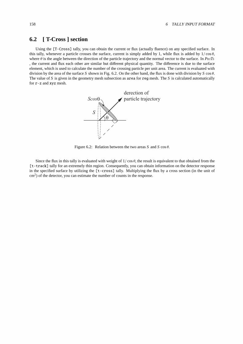
158 6 TALLY INPUT FORMAT
6.2 [ T-Cross ] section
Using the[T-Cross] tally, you can obtain the current or flux (actually fluence) on any specified surface. Inthis tally, whenever a particle crosses the surface, current is simply added by 1, while flux is added by 1/ cosθ,whereθ is the angle between the direction of the particle trajectory and the normal vector to the surface. InPHITS
, the current and flux each other are similar but different physical quantity. The difference is due to the surfaceelement, which is used to calculate the number of the crossing particle per unit area. The current is evaluated withdivision by the area of the surfaceS shown in Fig.6.2. On the other hand, the flux is done with division byS cosθ.The value ofS is given in the geometry mesh subsection asarea for regmesh. TheS is calculated automaticallyfor r-z andxyzmesh.
θ
Scosθ
S
derection of
particle trajectory
Figure 6.2: Relation between the two areasS andS cosθ.
Since the flux in this tally is evaluated with weight of 1/ cosθ, the result is equivalent to that obtained from the[t-track] tally for an extremely thin region. Consequently, you can obtain information on the detector responsein the specified surface by utilizing the[t-cross] tally. Multiplying the flux by a cross section (in the unit ofcm2) of the detector, you can estimate the number of counts in the response.

6.2 [ T-Cross ] section 159
Table 6.4:[t-cross] parameter (1)
name value explanation
mesh = reg, r-z, xyz geometry meshyou need geometry mesh subsection below this option
part = all (default), maximum 6 particles in a [t-cross]particle name
e-type = 1, 2, 3, 4, 5 energy meshYou need energy mesh subsection below this option
a-type = 1, 2, -1, -2 angle mesh (1, 2 :cos, -1, -2 :degree)The option is required You need angle mesh subsection below this optionfor a-curr and oa-curr
t-type = 1, 2, 3, 4, 5 time mesh(omissible) You need time mesh subsection below this option
unit = 1, 2, 3, 4, 5, 6 1: [1/cm2/source]2: [1/cm2/MeV/source]3: [1/cm2/Lethargy/source]4: [1/cm2/sr/source]5: [1/cm2/MeV/sr/source]6: [1/cm2/Lethargy/sr/source]
11, 12, 13, 14, 15, 16 11: [1/cm2/nsec/source]12: [1/cm2/MeV/nsec/source]13: [1/cm2/Lethargy/nsec/source]14: [1/cm2/sr/nsec/source]15: [1/cm2/MeV/sr/nsec/source]16: [1/cm2/Lethargy/sr/nsec/source]
axis = eng, reg, x, y, z, r x axis value of output datacos, the, t angle (cos, the) and time (t) meshxy, yz, xz 2 dimensional
There may be cases where results of tally are not correct, when a surface of mesh inr-z or xyz agrees withthat of the defined cell.
You can obtain current for specified angles using the angle mesh shown in Fig.6.3. In the cases ofunit=4,5, 6, 14, 15, or 16, the output is given as a quantity per solid angle (in steradian) calculated by using themesh size of the angle-bin defined in the angle mesh subsection.
θ
Figure 6.3: Schematic image of the tally using the angle mesh.
“Lethargy ” in unit = 3, 6, 13 or 16 is a natural logarithmic unit of energy, and defined by ln(Eref/E)using a reference energyEref and a particle’s energyE. If you set these units, you can obtain results per Lethargy,which are calculated by Lethargy widths, ln(Ehigh/Elow), at each energy bins given in the energy mesh subsection.Here,Ehigh andElow are maximum and minimum values of the energy bins, respectively.
“sr ” in unit = 4, 5, 6, 14, 15, or 16 denotes steradian, unit of solid angle.

160 6 TALLY INPUT FORMAT
Table 6.5:[t-cross] parameter (2)
name value explanation
file = file name Define file names as same number of axisresfile= (omissible,D=file) Define a file name of the past tally in the restart calculation.
Even if severalaxis parameters were defined, you shouldspecify only oneresfile.
multiplier = number of material multiplier for each material(omissible) You need multiplier subsection below this option
factor = (omissible, D=1.0) normalization factortitle = (omissible) titleangel = (omissible) angel parameters2d-type = 1, 2, 3, 4, 5, 6, 7 options for 2 dimensional plot
(omissible)output = flux flux by surface crossing
current current by surface crossingf-curr forward current by surface crossingb-curr backward current by surface crossingo-curr omni current by surface crossing
omni means the energy integratedof-curr omni forward current by surface crossingob-curr omni backward current by surface crossinga-curr angle mesh current by surface crossingoa-curr angle mesh omni current by surface crossing
x-txt = (omissible) x axis titley-txt = (omissible) y axis titlez-txt = (omissible) z axis titlegshow = 0 (default),1, 2, 3, 4 When mesh=xyz, axis=xy,yz,xz,
region border (1), material name (2), region name (3),and LAT number(4) are plotted by the option.
ginfo = 0 (default), No geometry check in the case of gshow>01 Check geometry and draw its two-dimensional view
with error information2 Check geometry, draw its two-dimensional view,
and outputting a geometry error file (.err)resol = 1 (default) The option multiplies region line resolution
by resol times with gshow option.width = 0.5 (default) The option defines the line thickness
for gshow option.epsout = 0 (default), 1, 2 Whenepsout=1, results are plotted into eps files.
This eps file is named by replacing the extension into “.eps ” .Whenepsout=2, error bars are also displayed in the eps file,except for 2 dimensional type (axis= xy, yz, xz).
ctmin(i) = (omissible, D=-9999) minimum value for i-th counterctmax(i) = (omissible, D= 9999) maximum value for i-th countertrcl = (omissible) coordinate transformation number or definition
for r-z or xyz meshdump = number of data Formesh=reg, the information is dumped on the file.
If dump is negative, data is written by ascii,if positive, by binary.
(next line) data sequence define the data sequence. The history information (nocasand nobch) is necessary to useidmpmode=1.
gslat = 1(default), 0 1: show lattice boundary in gshow, 0: no

6.2 [ T-Cross ] section 161
Output options, output=f-curr, b-curr, of-curr, ob-curr, can be used in xyz or r-z mesh. Note that in xyz meshthese options are available only for z-direction.
In the[t-cross] tally, you can use the dump option only withregmesh, and only withreg axis. If the dumpoption is set, the meshes ofe-type, a-type andt-type have only the meaning of the maximum and minimumvalues. The output option is set to be current,a-curr or oa-curr. When you use this dump parameter,axisandfile are restricted to one axis and one file, andunit is always 1. The dumped data are written on a filenamed “*** dmp”, where “***” indicates the file name specified by “file=***”. The normal output of the tallyis written on “***” . From this file, you can get the information on the total normalization factor. To do so, youhad better set one mesh fore-type, a-type andt-type. (In the former version of PHITS (before 2.66), thenormal output was written on a configuration file (.cfg), and the dumped data were written on “***” .) The historyinformation (nocas and nobch) is necessary to useidmpmode=1 for the continuous calculation using dump file.In addition, both of the two files, the dump file with “dmp” and the normal output file specified byfile=, arerequired to useidmpmode=1. The optiondumpall is not compatible with this dump tally option when sharedmemory parallelization is active.
If you setmesh = reg for geometry mesh in this section, you must define crossing surface by outgoing (r-in)and incoming (r-out) region number as an example below. Note that ”in” and ”out” is reversed in this definition.
mesh = reg
reg = number of crossing surfacesr-in r-out area
2 8 10.0
3 8 5.0
( 4 5 ) ( 4 5 ) 2.0
(13<5) (14<5) 7.0
(13<6) (14<6) 7.0
(13<7) (14<7) 7.0
... ... ....
... ... ....
The default order for this definition is “r-in r-out area”. If you want to change the order, define as“r-in r-out area”. You can use the skip operatornon. You can use the format( 2 - 5 8 9 ), and youcan use the lattice and universe style as( 6 < 10[1 0 0] < u=3 ). But you need to close a value by( )
if it is not a single numeric value. If you setoutput = flux, obtained flux is one way from r-in to r-out. If youwant to set both way flux, set as the third line of above definition.
If you setmesh = r-z, two kinds of crossing surface are defined. One is the number of “nz+1” crossingsurfaces for z defined byr i − r i+1. The other is the number of “nr+1” crossing surfaces for r defined byzi − zi+1. Ifr-surface coincides with the surface of outer void, the flux on this surface is not tallied.
If you setmesh=xyz, the number of “nz+1” crossing surfaces for z are defined byxi − xi+1 andy j − y j+1. Inthis case, x and y crossing surfaces are not defined. When you setmesh = rz, xyz, crossing particles are detectedin both ways at defined surface. The forward definitions are, positive direction in z surface, and from center tooutside in r surface.
From ver. 2.86,multiplier option can be used in[t-cross] tally.
Usingmultiplier option in this tally, you can multiply results of the tally by factors depending on energiesof particles. If you define a data set in[multiplier] section, any factors can be used. The basic format is givenas (C k), whereC is a normalization factor andk is the ID number of the set. It is noted thatk should be negative.Format of themultiplier subsection is given as follows.

162 6 TALLY INPUT FORMAT
multiplier = number of materialpart = neutron
emax = 1000
mat mset1 mset2
1 ( 1 -201 ) ( 2 -202 )
2 ( 1.2 -201 ) ( 3 -202 )
.... .... .... ....
.... .... .... ....
The line ofmultiplier = specifies the number of material where the multiplication is considered. You can useall instead of the number. For this case, one should also useall for mat column below. The second line ofpart= defines the particles considered. The maximum number of the particle is 6 andall can be also used, which isdefault. The multiplication affects only these considered particles. The third line ofemax = defines the maximumenergy of the multiplication. Ifemax is omitted, it is automatically defined as the maximum energy given in the[multiplier] section, ordmax(i), i = 1, 2, or 14 when you use nuclear data library. The number ofmatcolumn is the material number which is considered to be multiplied. The columns ofmset1, mset2 define themultiplier set. The maximum 6 multiplier can be set. For each set, the result is printed out. You can define severalmultiplier subsections in one[t-track] section, but you should set the number of the multiplier sets to beequal in each subsection.
Some parameter sets built-inPHITS can be used. If you setk = −1, a value of 1/weight is used as the multi-plication factor. Fork = −2, a value of 1/velocity is used. Fork = −120, material density is used. Therefore, youcan obtain mass in the region settingicntl=5. With k = −101,−102,−112, or−114, the conversion factor of pro-ton, neutron, electron, or photon, respectively, is used. These conversion factors were estimated with a conditionof Antero-Posterior geometry (AP) irradiation.7) The unit of the dose conversion factors is (µSv/h)/(n/sec/cm2).It should be noted that the interpolation method of conversion factor has been changed inPHITS ver. 2.00 fromlinear-linear to log-log.
You can also use the following format.
multiplier = number of materialpart = proton
emax = 150
mat mset1 mset2
1 ( 0.1236 1 1 -4 ) ( 0.0 )
2 ( 0.0060 2 1 -4 ) ( 0.0 )
3 ( 0.0032 3 1 -4 ) ( 0.0 )
.... .... .... ....
.... .... .... ....
multiplier = number of materialpart = neutron
emax = 150
mat mset1 mset2
1 ( 0.1236 1 1 -4 : -6 -8 ) ( 1.0 -1 33 0.543 )
2 ( 0.0060 2 1 -4 : -6 -8 ) ( 1.0 -1 34 0.321 )
3 ( 0.0032 3 1 -4 : -6 -8 ) ( 1.0 -1 35 0.678 )
.... .... .... ....
.... .... .... ....
In above example, themset1 is for heat and themset2 is zero for proton, attenuator set for neutron.

6.3 [ T-Point ] section 163
6.3 [ T-Point ] section
It is impractical to calculate particle fluence at a certain point or line, using[t-track] tally. Hence, the pointestimator tally[t-point] was introduced to estimate such quantities in a short computational time. However, thefollowing conditions must be satisfied in the PHITS simulation using[t-point]:
(1) Particle energy should not exceed the maximum energy of the data library used, i.e.dmax
(2) Only fluence of neutron and photon can be calculated by[t-point]
(3) Neither event generator mode nor EGS5 should not be used (e-mode=0, negs=0)
(4) Material should be uniform within a certain distance around the point detector due to singularity.
Please see read-me file or sample input file in\phits\utility\tpoint in more detail.
Table 6.6:[t-point] parameter(1)
name value explanation
point = number of data Option for point detectors.
You need subsection below this parameter.
ring = number of data Option for ring detectors.
You need subsection below this parameter.
part = all (default), maximum 6 particles in a [t-point]
particle name
e-type = 1, 2, 3, 4, 5 energy mesh
You need energy mesh subsection below this option
t-type = 1, 2, 3, 4, 5 time mesh
(omissible) You need time mesh subsection below this option
unit = 1, 2, 3 1: [1/cm2/source]
2: [1/cm2/MeV/source]
3: [1/cm2/Lethargy/source]
11, 12, 13 11:[1/cm2/nsec/source]
12:[1/cm2/nsec/MeV/source]
13:[1/cm2/Lethargy/nsec/source]
axis = eng, t x axis of output data
file = file name Define file names as same number of axis
resfile = (omissible, D=file) Define a file name of the past tally in the
restart calculation. Even if several axis
parameters were defined, you should specify only
one resfile.
multiplier = number of material multiplier for each material
(omissible) You need multiplier subsection below this option
factor = (omissible, D=1.0) normalization factor
title = (omissible) title
angel = (omissible) angel parameters
epsout = 0 (default), 1 If epsout is set to 1, results are plotted
into eps files. This eps file name is
named by replacing the extension into ‘‘.eps’’.
ctmin(i) = (omissible, D=-9999) minimum value for i-th counter
ctmax(i) = (omissible, D= 9999) maximum value for i-th counter
“Lethargy ” in unit = 3 or 13 is a natural logarithmic unit of energy, and defined by ln(Eref/E) using areference energyEref and a particle’s energyE. If you set these units, you can obtain results per Lethargy, whichare calculated by Lethargy widths, ln(Ehigh/Elow), at each energy bins given in the energy mesh subsection. Here,Ehigh andElow are maximum and minimum values of the energy bins, respectively.

164 6 TALLY INPUT FORMAT
In [t-point], you have to define the number of points or rings, instead ofmesh in other tallies. For example,you have to writepoint = 3 when you would like to define 3 point detectors. The maximum number of points orrings per[t-point] is 20. If you would like to set more detectors, you have to define another[t-point] tally.The point and ring detectors cannot be combined in one[t-point] tally. The information on each point and ringmust be defined in the successive lines after the definition ofpoint or ring parameter. The definition of the pointdetector is described as follows:
[ T-point ]
point = 1 # number of point detectors
non x y z r0
1 10.0 0.0 50.0 1.0
wherex, y, z indicate the coordinate of the point detector,r is the radius of the fictitious sphere. (About thefictitious sphere, see the read-me file in\phits\utility\tpoint .) The unit of these parameters are in cm.
The definition of the ring detector is defined as follows:
[ T-point ]
ring = 1 # number of ring detectors
non axis ar rr r0
1 z 50.0 10.0 1.0
whereaxis indicates the direction of ring axis specified byx, y or z, ar is the distance from the origin to thecenter of the ring,rr is the ring radius, andr0 is the radius of the fictitious sphere. You can change the order ofthese parameters by change the order of its denotation, e.g.x y z r0 to z y x r0. Except for this information,the parameters to be defined in[t-point] are the same as those in[t-track], including the multiplier option.Thus, radiation dose at a certain point can be estimated using[t-point]. However, you cannot specify material,two-dimensional plot option, and transform in[t-point].
Usingmultiplier option in this tally, you can multiply results of the[t-point] tally by factors dependingon energies of particles. If you define a data set in[multiplier] section, any factors can be used. The basicformat is given as (C k), whereC is a normalization factor andk is the ID number of the set. It is noted thatkshould be negative. Format of themultiplier subsection is given as follows.
multiplier = number of materialpart = neutron
emax = 1000
mat mset1 mset2
1 ( 1 -201 ) ( 2 -202 )
2 ( 1.2 -201 ) ( 3 -202 )
.... .... .... ....
.... .... .... ....
The line ofmultiplier = specifies the number of material where the multiplication is considered. You can useall instead of the number. For this case, one should also useall for mat column below. The second line ofpart= defines the particles considered. The maximum number of the particle is 6 andall can be also used, which isdefault. The multiplication affects only these considered particles. The third line ofemax = defines the maximumenergy of the multiplication. Ifemax is omitted, it is automatically defined as the maximum energy given in the[multiplier] section, ordmax(i), i = 1, 2, or 14 when you use nuclear data library. The number ofmatcolumn is the material number which is considered to be multiplied. The columns ofmset1, mset2 define themultiplier set. The maximum 6 multiplier can be set. For each set, the result is printed out. You can define severalmultiplier subsections in one[t-point] section, but you should set the number of the multiplier sets to be

6.3 [ T-Point ] section 165
equal in each subsection.Some parameter sets built-inPHITS can be used. If you setk = −1, a value of 1/weight is used as the multi-
plication factor. Fork = −2, a value of 1/velocity is used. Fork = −120, material density is used. Therefore, youcan obtain mass in the region settingicntl=5. With k = −101,−102,−112, or−114, the conversion factor of pro-ton, neutron, electron, or photon, respectively, is used. These conversion factors were estimated with a conditionof Antero-Posterior geometry (AP) irradiation.7) The unit of the dose conversion factors is (µSv/h)/(n/sec/cm2).It should be noted that the interpolation method of conversion factor has been changed inPHITS ver. 2.00 fromlinear-linear to log-log.
You can also use the following format.
multiplier = number of materialpart = proton
emax = 150
mat mset1 mset2
1 ( 0.1236 1 1 -4 ) ( 0.0 )
2 ( 0.0060 2 1 -4 ) ( 0.0 )
3 ( 0.0032 3 1 -4 ) ( 0.0 )
.... .... .... ....
.... .... .... ....
multiplier = number of materialpart = neutron
emax = 150
mat mset1 mset2
1 ( 0.1236 1 1 -4 : -6 -8 ) ( 1.0 -1 33 0.543 )
2 ( 0.0060 2 1 -4 : -6 -8 ) ( 1.0 -1 34 0.321 )
3 ( 0.0032 3 1 -4 : -6 -8 ) ( 1.0 -1 35 0.678 )
.... .... .... ....
.... .... .... ....
In above example, themset1 is for heat and themset2 is zero for proton, attenuator set for neutron.

166 6 TALLY INPUT FORMAT
6.4 [ T-Heat ] section
[ T - H e a t ] gives deposit energy for optional region. Deposit energy by low energy neutron and photon canbe also tallied in this tally. The heat from neutrons is usually obtained from Kerma factors with nuclear data. Fore-mode≥1, the heat from neutrons is zero, but the heat is calculated from energy loss of all charged particles andnuclei. The heat from photons is usually obtained also from Kerma factors with nuclear data. Forelectron=1
with electron transport, we do not use the Kerma factors of photon, but obtain the heat from the energy loss ofelectrons.
Table 6.7:[t-heat] parameter (1)
name value explanation
mesh = reg, r-z, xyz geometry meshyou need geometry mesh subsection below this option
axis = reg, x, y, z, r, x axis value of output dataxy, yz, xz, rz 2 dimensional
file = file name Define file names as same number of axisresfile= (omissible,D=file) Define a file name of the past tally in the restart calculation.
Even if severalaxis parameters were defined, you shouldspecify only oneresfile.
material = (omissible) You can specify materials for scoring.all, all : default (same as no definition)number of materials When you set number of materials,
define these material numbers in the next line.You can set number of materials by negative.In the case, specified materials are not includedfor scoring.
(next line) 2 5 8 material numbersoutput = heat total: Total deposit energy.
simple total: Total deposit energy.ncut, gcut, pcut: Deposit energies of neutrons, photons, and protonsbelow cut off energy when you setincut>0, igcut>0, ipcut>0,respectively.leakage: Kinetic energy of particles going out to the outer region.And, total: Total deposit energy.recoil: Kinetic energy of residual nuclei when you set cut offenergyemin(15-19).ionization: Deposit energy by energy-loss of charged particles.low neutron: Deposit energy calculated by neutron Kerma factors.photon: Deposit energy by Kerma factors.(If electron=1, contributions of electrons below cut off energy.)others: Excitation energy of residual nuclei. When you setigamma=1, this value comes to be 0 owing to photon emission.
Neutrons, photons, and protons below cut off energy, are not tallied in thencut, gcut, andpcut component,but in the stopped particle ifincut=0, igcut=0, andipcut=0 in the parameter section. Whenincut>0, igcut>0,andipcut>0, they are tallied in thencut, gcut, pcut part.

6.4 [ T-Heat ] section 167
Table 6.8:[t-heat] parameter (2)
name value explanation
output = all In addition to above,(continued) Contributions ofd, t,3He,α, and residual nuclei to recoil.
Contributions ofp, π+, π−, and the others to ionization.(Contributions of particles specified bypart are output.However, they are not plotted in eps file.)stopped particle: Kinetic energy of stopped proton, neutron,π+, π−, and the other particles in materials.(Contributions of particles specified bypart are output.However, they are not plotted in eps file.)others: Remaining excitation energy and fission component.Whenaxis is 2 dimensional,all is the same assimple.Only total, recoil, ionization, low neutron, electron, and othersare output.
part = particle name When you setoutput=all, deposit energies for ionization(omissible) and stopped particle specified here are output. It should be
noted that the results are not plotted in eps file.(omissible) ionization and stopped particle are used as output
unit = 0, 1, 2 0: [Gy/source]1: [MeV/cm3/source]2: [MeV/source]
factor = (omissible, D=1.0) normalization factortitle = (omissible) titleangel = (omissible) angel parameters2d-type = 1, 2, 3, 4, 5, 6, 7 options for 2 dimensional plot
(omissible)x-txt = (omissible) x axis titley-txt = (omissible) y axis titlez-txt = (omissible) z axis titlegshow = 0 (default),1, 2, 3, 4 When mesh=xyz, axis=xy,yz,xz,
region border (1), material name (2), region name (3),and LAT number(4) are plotted by the option.
rshow = 0 (default),1, 2, 3 When mesh=reg, axis=xy,yz,xz,region border (1), material name (2), and region name (3)are plotted by the option.You need xyz mesh section below this option.
ginfo = 0 (default), No geometry check in the case of gshow or rshow>01 Check geometry and draw its two-dimensional view
with error information2 Check geometry, draw its two-dimensional view,
and outputting a geometry error file (.err)resol = 1 (default) The option multiplies region line resolution
by resol times with gshow or rshow option.width = 0.5 (default) The option defines the line thickness
for gshow or rshow option.

168 6 TALLY INPUT FORMAT
Generally speaking, heat is an energy of ionization of charged particles. However, in the transport simulation,cutoff energy of the particle is set and the transport is stopped below the energy. Then there exist some componentsof heat, i.e. recoil, stopped particle, and others, in the output of the heat tally. These components may change asthe parameters of the transport are changed.
Table 6.9:[t-heat] parameter (3)
name value explanation
volume (omissible) The option defines volume for each regionfor reg mesh. You need volume definitionsbelow this option.Default values are given in inputecho in the case of no definition.
reg vol volume definition. See5.1.2iechrl = 72 (default) Number of maximum column for volume input echovolmat = (omissible, D=9) The option corrects a volume value for each mesh
when material is defined by xyz mesh.(0 means no correction)Value of volmat means the number of scansfor one side of xyz mesh
epsout = 0 (default), 1 If epsout is set to 1, results are plottedinto eps files. This eps file is namedby replacing the extension into “.eps”.
bmpout = 0(default), 1 Generate Bitmap figure of 2-dimensional tally output.This file is named by replacing the extension into “.bmp ” .Whenmesh=xyz, axis=(xy, yz, or xz), this is available.
vtkout = 0(default), 1 Output the tally results in xyz-mesh in the input format of ParaView.This file is named by replacing the extension into “.vtk ” .Whenmesh=xyz, axis=(xy, yz, or xz), this is available.
vtkfmt = 0(default), 1 Format of output file for ParaView.0: ascii, 1: binary.
electron = 0 (default),1 electron contribution options0: using photon KERMA factors(electron and positron should NOT be transported,otherwise their deposition energies are double counted)1: calculating by ionization loss(electron and positron transports are required)
ctmin(i) = (omissible, D=-9999) minimum value for i-th counterctmax(i) = (omissible, D= 9999) maximum value for i-th countertrcl = (omissible) coordinate transformation number or definition
for r-z or xyz meshgslat = 1(default), 0 1: show lattice boundary in gshow, 0: no
When you setunit = 0, you can obtain results in the unit of [Gy/source]. When you setmesh = reg, youshould define volumes of each cells in [volume] section or by settingvolume parameter of the [t-heat] section.Because absorbed dose is intensive variable,PHITS does not output “sum over”in output files forunit = 0. Itshould be noted that when a region includes more than two materials, dose in the region does not equal to averagevalue of the region. For example, when two material with massesM1 & M2, and absorb energiesE1 & E2,respectively,PHITS gives E1
M1+ E2
M2in this tally, though its average dose isE1+E2
M1+M2.

6.5 [ T-Deposit ] section 169
6.5 [ T-Deposit ] section
This tally is very similar to [t-heat] and scores dose and deposit energy distributions. The difference from[t-heat] is that this tally only counts an energy loss of charged particles and nuclei. Thus, you must use the eventgenerator mode (e-mode≥1) if you would like to transport low-energy neutrons. In this tally, you can multiply anyfactor as a function of LET(dE/dx) in a certain material to the dose or deposit energy. This function is realizedby user defined subroutine usrdfn1.f and usrdn2.f. As examples, the default program of usrdfn1.f returns the doseequivalent calculated from deposit energy multiplied with theQ(L) relationship defined in the ICRP60, while thatof usrdfn2.f simply does the energy loss without multiplying any factor. You can change and add any factor in thisroutine. In addition, using the time mesh with [timer] section, you can simulate a TOF (time of flight) detector andplot 2-dimensional graph of the correlation between the deposit energy and the TOF. Whenoutput = deposit
is set, you can simulate the detector response. Note that you cannot use this tally when a particle weight changesin the calculation by using[weight window] etc. After version 2.70, the detector resolution can be consideredin the calculation of event-by-event deposition-energy distributions usingoutput = deposit.
Table 6.10:[t-deposit] parameters(1)
name value explanation
mesh = reg, r-z, xyz geometry meshyou need geometry mesh subsection below this option
part = all (default), maximum 6 particles in a[t-deposit]particle name Whenoutput=deposit anddeposit=0, all is necessary
and you can set only maximum 5 particles.material = (omissible) You can specify materials for scoring.
all, all : default (same as no definition)number of materials When you set number of materials,
define these material numbers in the next line.You can set number of materials by negative.In the case, specified materials are not includedfor scoring.
(next line) 2 5 8 material numbersletmat = (omissible) material id for LET(dE/dx).
If omitted, real material is assumed.If you select the material that is not used in your geometry,you have to define its material density in [material] section.If you would like to calculate LET in water, you have todefine water with 1 g/cm3 in [material] sectiont.When you set letmat< 0, PHITS automatically calculatesdE/dx for water with 1 g/cm3 for electrons and positrons.Please see “particletherapy” in the recommendation settingin more detail.
dedxfnc= (omissible, D=0) 0: without, 1: use usrdfn1.f, 2: use usrdfn2.fAs examples, the default program of usrdfn1.f returns the doseequivalent calculated from deposit energy multiplied with theQ(L) relationship defined in the ICRP60, while that of usrdfn2.fsimply does the energy loss without multiplying any factor.
e-type = 1, 2, 3, 4, 5 energy meshYou need energy mesh subsection below this option.
t-type = 1, 2, 3, 4, 5 time mesh(omissible) You need time mesh subsection below this option.

170 6 TALLY INPUT FORMAT
Table 6.11:[t-deposit] parameter (2)
name value explanation
output= dose score the energy loss of charged particles and nucleideposit score deposit energy distribution
You neede-type subsection.unit = 0, 1, 2, 3, 4 0: Dose [Gy/source]; only foroutput=dose
1: Dose [MeV/cm3/source]2: Dose [MeV/source]3: Number [1/source]; only foroutput=deposit4: Number [1/nsec/source]; only foroutput=deposit
deposit= 0(default), 1 Option for deposit energy plot when output=deposit.0: distribution of total deposit energy with contributionof each particle. (Please use this setting normally)1: distribution of deposit energy caused by each particle.(default setting until ver. 2.81)
axis = eng, reg, x, y, z, x axis value of output datar, t
xy, yz, xz, rz 2 dimensionalt-eng, eng-t
file = file name Define file names as same number of axisresfile= (omissible,D=file) Define a file name of the past tally in the restart calculation.
Even if severalaxis parameters were defined, you shouldspecify only oneresfile.
factor = (omissible, D=1.0) normalization factortitle = (omissible) titleangel = (omissible) angel parameters2d-type = 1, 2, 3, 4, 5, 6, 7 options for 2 dimensional plot
(omissible)x-txt = (omissible) x axis titley-txt = (omissible) y axis titlez-txt = (omissible) z axis titlegshow = 0 (default),1, 2, 3, 4 When mesh=xyz, axis=xy,yz,xz,
region border (1), material name (2), region name (3),and LAT number(4) are plotted by the option.
rshow = 0 (default),1, 2, 3 When mesh=reg, axis=xy,yz,xz,region border (1), material name (2), and region name (3)and LAT number(4) are plotted by the option.You need xyz mesh section below this option.
In this tally, one can only score the energy loss of charged particles. So you cannot get the sum of the energyloss for a specific particle which goes into the tally region by usingpart = in this tally section. In order to tallythe energy loss for each projectile particle going into the tally region, you should define the counter withpart =
in [counter] section andctmin, ctmax in this tally section.When you setunit = 0 with output = dose, you can obtain results in the unit of [Gy/source]. When you
setmesh = reg, you should define volumes of each cells in [volume] section or by settingvolume parameter ofthe [t-heat] section. Because absorbed dose is intensive variable,PHITS does not output “sum over”in output filesfor unit = 0. It should be noted that when a region includes more than two materials, dose in the region does notequal to average value of the region. For example, when two material with massesM1 & M2, and absorb energiesE1 & E2, respectively,PHITS gives E1
M1+ E2
M2in this tally, though its average dose isE1+E2
M1+M2.

6.5 [ T-Deposit ] section 171
When you setoutput = deposit anddeposit = 0, you can obtain the contribution of each kind of particleset inpart to the result ofall. In this case, if you don’t setall in part, part = all is automatically set.
When you setoutput = deposit anddeposit = 1, you can obtain the distribution of energies deposited byeach kind of particle set inpart. Therefore, a sum of results obtained by settingpart = individual particledoes not equal to the distribution of energies deposited byall.
In the case ofoutput = deposit anddeposit = 0, statistical uncertainties of results except for values ofpart = all are standard deviations calculated by the history variance mode, independent ofistdev.
Although the fano factor is generally defined as a dimensionless quantity,dfano parameter is defined as aquantity with a dimension of energy.

172 6 TALLY INPUT FORMAT
Table 6.12:[t-deposit] parameter (3)
name value explanation
ginfo = 0 (default), No geometry check in the case of gshow or rshow>01 Check geometry and draw its two-dimensional view
with error information2 Check geometry, draw its two-dimensional view,
and outputting a geometry error file (.err)resol = 1 (default) The option multiplies region line resolution
by resol times with gshow or rshow option.width = 0.5 (default) The option defines the line thickness
for gshow or rshow option.volume (omissible) The option defines volume for each region for reg mesh.
You need volume definitions below this option. Defaultvalues are given in input echo in the case of no definition.
reg vol volume definition. See5.1.2iechrl = 72 (default) Number of maximum column for volume input echovolmat = (omissible, D=9) The option corrects a volume value for each mesh
when material is defined by xyz mesh.(0 means no correction)Value of volmat means the number of scansfor one side of xyz mesh
epsout = 0 (default), 1, 2 Whenepsout=1, results are plotted into eps files.This eps file is named by replacing the extension into “.eps ” .Whenepsout=2, error bars are also displayed in the eps file,except for 2 dimensional type (axis= xy, yz, xz, rz).
bmpout = 0(default), 1 Generate Bitmap figure of 2-dimensional tally output.This file is named by replacing the extension into “.bmp ” .Whenmesh=xyz, axis=(xy, yz, or xz), this is available.
vtkout = 0(default), 1 Output the tally results in xyz-mesh in the input format of ParaView.This file is named by replacing the extension into “.vtk ” .Whenmesh=xyz, axis=(xy, yz, or xz), this is available.
vtkfmt = 0(default), 1 Format of output file for ParaView.0: ascii, 1: binary.
ctmin(i) = (omissible, D=-9999) minimum value for i-th counterctmax(i) = (omissible, D= 9999) maximum value for i-th countertrcl = (omissible) coordinate transformation number or definition
for r-z or xyz meshgslat = 1(default), 0 1: show lattice boundary in gshow, 0: nodresol (omissible, D=0.0) Parameter for representing the detector resolution.
Valid only for output = deposit. When you setdresol=σr
anddfano=F, deposition energyE of each event is fluctuatedby following the Gaussian with standard deviation
√σ2
r + FE.dfano (omissible, D=0.0) Parameter for representing the detector resolution.
Valid only for output = deposit. When you setdresol=σr
anddfano=F, deposition energyE of each event is fluctuatedby following the Gaussian with standard deviation
√σ2
r + FE.

6.6 [ T-Deposit2 ] section 173
6.6 [ T-Deposit2 ] section
This tally scores deposit energy distribution in two regions and plot the correlation between two deposit ener-gies. By this, one can simulate, for an example, dE, E counters and plot the correlations in 2-dimensional graph.Using this tally, you can simulate the detector response. Note that you cannot use this tally when a particle weightchanges in the calculation by using[weight window] etc. In this tally, as in the [t-deposit] tally, you can multiplyany factor as a function of LET(dE/dx) in a certain material to the dose or deposit energy. This function is realizedby user defined subroutine usrdfn1.f and usrdn2.f. As examples, the default program of usrdfn1.f returns the doseequivalent calculated from deposit energy multiplied with theQ(L) relationship defined in the ICRP60, while thatof usrdfn2.f simply does the energy loss without multiplying any factor. You can change and add any factor in thisroutine. In addition, using the time mesh with [timer] section, you can simulate a TOF (time of flight) detector andplot 2-dimensional graph of the correlation between the deposit energy and the TOF.
Table 6.13:[t-deposit2] parameters(1)
name value explanation
mesh = reg geometry mesh, onlyregreg = r1 r2 Two region numbers should be written.part = all (default), maximum 6 particles in a [t-deposit2]
particle nameletmat1 = (omissible) material id for LET(dE/dx) of region r1
If omitted, real material is assumed.letmat2 = (omissible) material id for LET(dE/dx) of region r2
If omitted, real material is assumed.If you select the material that is not used in your geometry,you have to define its material density in [material] section.If you would like to calculate LET in water, you have todefine water with 1 g/cm3 in [material] sectiont.When you set letmat< 0, PHITS automatically calculatesdE/dx for water with 1 g/cm3 for electrons and positrons.Please see “particletherapy” in the recommendation settingin more detail.
dedxfnc1= (omissible, D=0) for region r1, 0: without,1: use usrdfn1.f, 2: use usrdfn2.f
dedxfnc2= (omissible, D=0) for region r2, 0: without,1: use usrdfn1.f, 2: use usrdfn2.fAs examples, the default program of usrdfn1.f returns the doseequivalent calculated from deposit energy multiplied with theQ(L) relationship defined in the ICRP60, while that of usrdfn2.fsimply does the energy loss without multiplying any factor.
e1-type = 1, 2, 3, 4, 5 energy mesh for region r1You need energy mesh subsection below this option
e2-type = 1, 2, 3, 4, 5 energy mesh for region r2You need energy mesh subsection below this option
t-type = 1, 2, 3, 4, 5 time mesh(omissible) You need time mesh subsection below this option
unit = 1, 2 1: Number [1/source]2: Number [1/nsec/source]
axis = eng1, eng2, t, x axis value of output datae12, e21, t-e1, t-e2 2 dimensionale1-t, e2-t
file = file name Define file names as same number of axisresfile= (omissible,D=file) Define a file name of the past tally in the restart calculation.
Even if severalaxis parameters were defined, you shouldspecify only oneresfile.

174 6 TALLY INPUT FORMAT
Table 6.14:[t-deposit2] parameter (2)
name value explanation
factor = (omissible, D=1.0) normalization factortitle = (omissible) titleangel = (omissible) angel parameters2d-type = 1, 2, 3, 4, 5, 6, 7 options for 2 dimensional plot
(omissible)x-txt = (omissible) x axis titley-txt = (omissible) y axis titlez-txt = (omissible) z axis titlevolume (omissible) The option defines volume for each region
for reg mesh. You need volume definitionsbelow this option.Default values are given in inputecho in the case of no definition.
reg vol volume definition. See5.1.2iechrl = 72 (default) Number of maximum column for volume input echoepsout = 0 (default), 1 If epsout is set to 1, results are plotted
into eps files. This eps file is namedby replacing the extension into “.eps”.
ctmin(i) = (omissible, D=-9999) minimum value for i-th counterctmax(i) = (omissible, D= 9999) maximum value for i-th counter
This tally only scores the energy loss of charged particles. So you cannot get the sum of the energy loss fora specific particle which goes into the tally region by usingpart = in this tally section. In order to tally theenergy loss for each projectile particle going into the tally region, you should define the counter withpart = in[counter] section andctmin, ctmax in this tally section.

6.7 [ T-Yield ] section 175
6.7 [ T-Yield ] section
[ T - Y i e l d ] gives information on produced nuclei. Products by neutrons in the energy belowdmax(2) arenot scored, but scored withe-mode≥1.
Table 6.15:[t-yield] parameter (1)
name value explanation
mesh = reg, r-z, xyz geometry meshyou need geometry mesh subsection below this option
special = D=0 (omissible) Whenspecial > 0, nuclear reactions are repeatedmore than once in order to increase statistics.
part = all (default), maximum 6 particles in a [t-yield]particle name projectile particle of the reaction
material = (omissible) You can specify materials for scoring.all, all : default (same as no definition)number of materials When you set number of materials,
define these material numbers in the next line.You can set number of materials by negative.In the case, specified materials are not includedfor scoring.
(next line) 2 5 8 material numbersmother = (omissible) You can specify mother nuclei.
all, all : default (same with no definition)number of mother nuclei When you set number of mother nuclei,
define their mothers in the next line.You can set number of mothers by negative.In this case, specified mothers are not includedfor scoring.
(next line) 208Pb Pb Nucleus if you specify with mass.Without mass, all isotopes of PbIf you want to specify multiple mother groups,use multiple [t-yield] tallies
nucleus = (omissible) You can specify output nuclei.all, all : default (same with no definition)number of nuclei When you set number of nuclei,
define their nuclei in the next line.(next line) 208Pb Pb Nucleus If you specify with mass.
Without mass, all isotopes of Pbelastic = 1(default),0,-1 Option for contribution of a recoil nucleus in elastic collisions
1: with this contribution0: exclude recoil target nucleus produced by elastic collisions-1: exclude the same nucleus as the target nucleus
unit = 1, 2 1: [1/source]2: [1/cm3/source]

176 6 TALLY INPUT FORMAT
Table 6.16:[t-yield] parameter(2)
name value explanation
ndata = 0(default),1 If you set 1, nuclear production cross section dataare used for nuclear irradiation in cases of proton inducedreactions onα, 14N, 16O targets as shown below.
axis = reg, x, y, z, r, x axis for outputxy, yz, xz, rz 2 dimensionmass Mass distribution. If the case nucleus is
specified, isotope distribution.charge Charge distribution. Nucleus cannot be specified.chart Nucleus chart (x:N, y:Z)。
Nucleus cannot be specifieddchain for dchain-sp output. All isotopes are output
only mesh= reg
For this tally, only oneaxis parameter is defined in a[t-yield] section.
file = file name Define a file name to output.resfile= (omissible,D=file) Define a file name of the past tally in the restart calculation.
Even if severalaxis parameters were defined, you shouldspecify only oneresfile.
output = (omissible) change the timing of the score.product (default) Nuclei produced by nuclear reaction are tallied.cutoff Nuclei stopped by energy cutoff are tallied.
If nuclei are not transported, this is the same asproductinfo = 0, 1 With stable nuclei and magic number for chart.factor = (omissible, D=1.0) normalization factortitle = (omissible) titleangel = (omissible) angel parameters2d-type = 1, 2, 3, 4, 5, 6, 7 options for 2 dimensional plot
(omissible)x-txt = (omissible) x axis titley-txt = (omissible) y axis titlez-txt = (omissible) z axis title
The following nuclear reactions are included in the available nuclear data for ndata=1
4He(n, x)3H 14N(n, x)3H 14N(n, x)7Be 14N(n, x)11Be 14N(n, x)10C 14N(n, x)11C14N(n, x)14C 14N(n, x)13N 16O(n, x)3H 16O(n, x)7Be 16O(n, x)11Be 16O(n, x)10C16O(n, x)11C 16O(n, x)14C 16O(n, x)15C 16O(n, x)13N 16O(n, x)16N 16O(n, x)14O16O(n, x)15O 4He(p, x)3H 14N(p, x)7Be 14N(p, x)11Be 14N(p, x)10C 14N(p, x)11C14N(p, x)13N 14N(p, x)14O 16O(p, x)3H 16O(p, x)7Be 16O(p, x)11Be 16O(p, x)10C16O(p, x)11C 16O(p, x)14C 16O(p, x)13N 16O(p, x)14O 16O(p, x)15O
If you specifyoutput=cutoff, the parameters ofpart, mother are neglected.Whenigamma=3 in [parameters] section, you can obtain information on the isomer production based on
EBITEM model by settingaxis=chart, dchain in this tally.

6.7 [ T-Yield ] section 177
Table 6.17:[t-yield] parameter (3)
name value explanation
gshow = 0 (default),1, 2, 3, 4 When mesh=xyz, axis=xy,yz,xz,region border (1), material name (2), region name (3),and LAT number(4) are plotted by the option.
rshow = 0 (default),1, 2, 3 When mesh=reg, axis=xy,yz,xz,region border (1), material name (2), and region name (3)are plotted by the option.You need xyz mesh section below this option.
ginfo = 0 (default), No geometry check in the case of gshow or rshow>01 Check geometry and draw its two-dimensional view
with error information2 Check geometry, draw its two-dimensional view,
and outputting a geometry error file (.err)resol = 1 (default) The option multiplies region line resolution
by resol times with gshow or rshow option.width = 0.5 (default) The option defines the line thickness
for gshow or rshow option.volume (omissible) The option defines volume for each region
for reg mesh. You need volume definitionsbelow this option.Default values are given in inputecho in the case of no definition.
reg vol volume definition. See5.1.2iechrl = 72 (default) Number of maximum column for volume input echovolmat = (omissible, D=9) The option corrects a volume value for each mesh
when material is defined by xyz mesh.(0 means no correction)Value of volmat means the number of scansfor one side of xyz mesh
epsout = 0 (default), 1 If epsout is set to 1, results are plottedinto eps files. This eps file is namedby replacing the extension into “.eps”.
bmpout = 0(default), 1 Generate Bitmap figure of 2-dimensional tally output.This file is named by replacing the extension into “.bmp ” .Whenmesh=xyz, axis=(xy, yz, or xz), this is available.
vtkout = 0(default), 1 Output the tally results in xyz-mesh in the input format of ParaView.This file is named by replacing the extension into “.vtk ” .Whenmesh=xyz, axis=(xy, yz, or xz), this is available.
vtkfmt = 0(default), 1 Format of output file for ParaView.0: ascii, 1: binary.
ctmin(i) = (omissible, D=-9999) minimum value for i-th counterctmax(i) = (omissible, D= 9999) maximum value for i-th countertrcl = (omissible) coordinate transformation number or definition
for r-z or xyz meshgslat = 1(default), 0 1: show lattice boundary in gshow, 0: no

178 6 TALLY INPUT FORMAT
6.8 [ T-Product ] section
[ T - P r o d u c t ] tallies particles and nuclei produced by nuclear reaction, decay, and fission, and also talliessource particles. The differences from [t-yield] are that you can get the energy distribution and time distributionof produced particles and nuclei. This tally is not available for low energy neutron, photon, and electron. Fore-mode≥1, however, particles and nuclei produced by reactions due to neutron with the library can be obtained.
Table 6.18:[t-product] parameter (1)
name value explanation
mesh = reg, r-z, xyz geometry meshyou need geometry mesh subsection below this option
part = all (default), maximum 6 particles in a [t-product]particle name
material = (omissible) You can specify materials for scoring.all, all : default (same as no definition)number of materials When you set number of materials,
define these material numbers in the next line.You can set number of materials by negative.In the case, specified materials are not includedfor scoring.
(next line) 2 5 8 material numbersmother = (omissible) You can specify mother nuclei.
all, all : default (same with no definition)number of mother nuclei When you set number of mother nuclei,
define their mothers in the next line.You can set number of mothers by negative.In this case, specified mothers are not includedfor scoring.
(next line) 208Pb Pb Nucleus if you specify with mass.Without mass, all isotopes of PbIf you want to specify multiple mother groups,use multiple [t-product] tallies.
e-type = 1, 2, 3, 4, 5 energy meshYou need energy mesh subsection below this option.
t-type = 1, 2, 3, 4, 5 time mesh(omissible) You need time mesh subsection below this option.
a-type = 1, 2, -1, -2 angle mesh (1, 2 :cos, -1, -2 :degree)You need angle mesh subsection below this option.

6.8 [ T-Product ] section 179
Table 6.19:[t-product] parameter (2)
name value explanation
unit = 1, 2, 3, 4, 5, 6 1: [1/source]2: [1/cm3/source]3: [1/MeV/source]4: [1/cm3/MeV/source]5: [1/Lethargy/source]6: [1/cm3/Lethargy/source]
11, 12, 13, 14, 15, 16 11:[1/nsec/source]12:[1/cm3/nsec/source]13:[1/MeV/nsec/source]14:[1/cm3/MeV/nsec/source]15:[1/Lethargy/nsec/source]16:[1/cm3/Lethargy/nsec/source]
21, 22, 23, 24, 25, 26 21: [1/sr/source]22: [1/cm3/sr/source]23: [1/MeV/sr/source]24: [1/cm3/MeV/sr/source]25: [1/Lethargy/sr/source]26: [1/cm3/Lethargy/sr/source]
31, 32, 33, 34, 35, 36 31:[1/nsec/sr/source]32:[1/cm3/nsec/sr/source]33:[1/MeV/nsec/sr/source]34:[1/cm3/MeV/nsec/sr/source]35:[1/Lethargy/nsec/sr/source]36:[1/cm3/Lethargy/nsec/sr/source]
“Lethargy ” in unit = 5, 6, 15, 16, 25, 26, 35 or 36 is a natural logarithmic unit of energy, anddefined by ln(Eref/E) using a reference energyEref and a particle’s energyE. If you set these units, you can obtainresults per Lethargy, which are calculated by Lethargy widths, ln(Ehigh/Elow), at each energy bins given in theenergy mesh subsection. Here,Ehigh andElow are maximum and minimum values of the energy bins, respectively.
“sr ” in unit = 21 - 26 or 31 - 36 denotes steradian, unit of solid angle.

180 6 TALLY INPUT FORMAT
Table 6.20:[t-product] parameter (3)
name value explanation
axis = eng, reg, x, y, z, r, x axis value of output dataxy, yz, xz, rz 2 dimensionalt time axis
file = file name Define file names as same number of axisresfile= (omissible,D=file) Define a file name of the past tally in the restart calculation.
Even if severalaxis parameters were defined, you shouldspecify only oneresfile.
output = source source particlenuclear (default) particles from nuclear reaction including elasticnonela particles from nonelastic collisionelastic particles from elastic collisiondecay particles from decayfission particles from fission
factor = (omissible, D=1.0) normalization factortitle = (omissible) titleangel = (omissible) angel parameters2d-type = 1, 2, 3, 4, 5, 6, 7 options for 2 dimensional plot
(omissible)x-txt = (omissible) x axis titley-txt = (omissible) y axis titlez-txt = (omissible) z axis titlegshow = 0 (default),1, 2, 3, 4 When mesh=xyz, axis=xy,yz,xz,
region border (1), material name (2), region name (3),and LAT number(4) are plotted by the option.
rshow = 0 (default),1, 2, 3 When mesh=reg, axis=xy,yz,xz,region border (1), material name (2), and region name (3)are plotted by the option.You need xyz mesh section below this option.
ginfo = 0 (default), No geometry check in the case of gshow or rshow>01 Check geometry and draw its two-dimensional view
with error information2 Check geometry, draw its two-dimensional view,
and outputting a geometry error file (.err)resol = 1 (default) The option multiplies region line resolution
by resol times with gshow or rshow option.width = 0.5 (default) The option defines the line thickness
for gshow or rshow option.volume (omissible) The option defines volume for each region
for reg mesh. You need volume definitionsbelow this option.Default values are given in inputecho in the case of no definition.
reg vol volume definition. See5.1.2iechrl = 72 (default) Number of maximum column for volume input echo

6.8 [ T-Product ] section 181
Table 6.21:[t-product] parameter (4)
name value explanation
volmat = (omissible, D=9) The option corrects a volume value for each meshwhen material is defined by xyz mesh.(0 means no correction)Value of volmat means the number of scansfor one side of xyz mesh.
epsout = 0 (default), 1, 2 Whenepsout=1, results are plotted into eps files.This eps file is named by replacing the extension into “.eps ” .Whenepsout=2, error bars are also displayed in the eps file,except for 2 dimensional type (axis= xy, yz, xz, rz).
bmpout = 0(default), 1 Generate Bitmap figure of 2-dimensional tally output.This file is named by replacing the extension into “.bmp ” .Whenmesh=xyz, axis=(xy, yz, or xz), this is available.
vtkout = 0(default), 1 Output the tally results in xyz-mesh in the input format of ParaView.This file is named by replacing the extension into “.vtk ” .Whenmesh=xyz, axis=(xy, yz, or xz), this is available.
vtkfmt = 0(default), 1 Format of output file for ParaView.0: ascii, 1: binary.
ctmin(i) = (omissible, D=-9999) minimum value for i-th counterctmax(i) = (omissible, D= 9999) maximum value for i-th countertrcl = (omissible) coordinate transformation number or definition
for r-z or xyz meshdump = number of data Formesh=reg, the information is dumped on the file.
If dump is negative, data are written by ascii,if positive, by binary.
(next line) data sequence define the data sequence. The history information (nocasand nobch) is necessary to useidmpmode=1.
gslat = 1(default), 0 1: show lattice boundary in gshow, 0: no
In the [t-product] tally, you can use the dump option. If the dump option is set, the meshes ofe-type
andt-type have only the meaning of the maximum and minimum values. When you use this dump parameter,axis andfile are restricted to one axis and one file, andunit is always 1. The dumped data are written on afile named “*** dmp”, where “***” indicates the file name specified by “file=***”. The normal output of thetally is written on “***” . From this file, you can get the information on the total normalization factor. To do so,you had better set one mesh fore-type, a-type andt-type. (In the former version of PHITS (before 2.66),the normal output was written on a configuration file (.cfg), and the dumped data were written on “***” .) Thehistory information (nocas and nobch) is necessary to useidmpmode=1 for the continuous calculation using dumpfile. In addition, both of the two files, the dump file with “dmp” and the normal output file specified byfile=,are required to useidmpmode=1. The optiondumpall is not compatible with this dump tally option when sharedmemory parallelization is active.
This [t-product] can tally the source particles. By using this function, you can modify the dump file. Youcan read a dump file and write the information on a new dump file with some modification by setting the dumpparameter andoutput = source in this tally section, andicntl = 6 in the parameter section.

182 6 TALLY INPUT FORMAT
6.9 [ T-DPA ] section
[ T - D P A ] gives DPA (Displacement Per Atom) value. This is the number of displaced atoms per a targetatom, and represents the radiation damage in materials irradiated by energetic particles. The result by this tallyincludes the contribution of Coulomb scattering cross section for the charged particle transportation. DPA by lowenergy neutron incident reactions can be also obtained by usinge-mode≥1.
Table 6.22:[t-dpa] parameter (1)
name value explanation
mesh = reg, r-z, xyz geometry meshyou need geometry mesh subsection below this option
part = all (default), maximum 6 particles in a [t-dpa]particle name
material = (omissible) You can specify materials for scoring.all, all : default (same as no definition)number of materials When you set number of materials,
define these material numbers in the next line.You can set number of materials by negative.In the case, specified materials are not includedfor scoring.
(next line) 2 5 8 material numbersmother = (omissible) You can specify mother nuclei.
all, all : default (same with no definition)number of mother nuclei When you set number of mother nuclei,
define their mothers in the next line.You can set number of mothers by negative.In this case, specified mothers are not includedfor scoring.
(next line) 208Pb Pb Nucleus if you specify with mass.Without mass, all isotopes of Pb.If you want to specify multiple mother groups,use multiple [t-dpa] tallies.
unit = 1, 2 1: [DPA*1.e-24/source]2: [DPA/source]
axis = eng, reg, x, y, z, r, x axis value of output dataxy, yz, xz, rz 2 dimensional
file = file name Define file names as same number of axisresfile= (omissible,D=file) Define a file name of the past tally in the restart calculation.
Even if severalaxis parameters were defined, you shouldspecify only oneresfile.

6.9 [ T-DPA ] section 183
Table 6.23:[t-dpa] parameter (2)
name value explanation
output = dpa total: total DPA valuecutoff1: DPA value when energies of charged particlesproduced by reactions are below cutoff energy (emin)cutoff2: DPA value when energies of charged particlestransported in materials are below cutoff energy (emin)transpt: DPA value when charged particles are transported
all add d, t,3He,α, and nucleus contributions as PKA,with “simple”
factor = (omissible, D=1.0) normalization factortitle = (omissible) titleangel = (omissible) angel parameters2d-type = 1, 2, 3, 4, 5, 6, 7 options for 2 dimensional plot
(omissible)x-txt = (omissible) x axis titley-txt = (omissible) y axis titlez-txt = (omissible) z axis titlegshow = 0 (default),1, 2, 3, 4 When mesh=xyz, axis=xy,yz,xz,
region border (1), material name (2), region name (3),and LAT number(4) are plotted by the option.
rshow = 0 (default),1, 2, 3 When mesh=reg, axis=xy,yz,xz,region border (1), material name (2), and region name (3)are plotted by the option.You need xyz mesh section below this option.
ginfo = 0 (default), No geometry check in the case of gshow or rshow>01 Check geometry and draw its two-dimensional view
with error information2 Check geometry, draw its two-dimensional view,
and outputting a geometry error file (.err)resol = 1 (default) The option multiplies region line resolution
by resol times with gshow or rshow option.width = 0.5 (default) The option defines the line thickness
for gshow or rshow option.volume (omissible) The option defines volume for each region
for reg mesh. You need volume definitionsbelow this option.Default values are given in inputecho in the case of no definition.
reg vol volume definition. See5.1.2iechrl = 72 (default) Number of maximum column for volume input echovolmat = (omissible, D=9) The option corrects a volume value for each mesh
when material is defined by xyz mesh.(0 means no correction)Value of volmat means the number of scansfor one side of xyz mesh.

184 6 TALLY INPUT FORMAT
Table 6.24:[t-dpa] parameter (3)
name value explanation
epsout = 0 (default), 1 If epsout is set to 1, results are plottedinto eps files. This eps file is namedby replacing the extension into “.eps”.
bmpout = 0(default), 1 Generate Bitmap figure of 2-dimensional tally output.This file is named by replacing the extension into “.bmp ” .Whenmesh=xyz, axis=(xy, yz, or xz), this is available.
vtkout = 0(default), 1 Output the tally results in xyz-mesh in the input format of ParaView.This file is named by replacing the extension into “.vtk ” .Whenmesh=xyz, axis=(xy, yz, or xz), this is available.
vtkfmt = 0(default), 1 Format of output file for ParaView.0: ascii, 1: binary.
ctmin(i) = (omissible, D=-9999) minimum value for i-th counterctmax(i) = (omissible, D= 9999) maximum value for i-th countertrcl = (omissible) coordinate transformation number or definition
for r-z or xyz meshgslat = 1(default), 0 1: show lattice boundary in gshow, 0: no

6.10 [ T-LET ] section 185
6.10 [ T-LET ] section
By the LET tally, you can get the information on track length and dose as a function of LET(dE/dx) of acertain material. This tally counts an energy loss of charged particles and nuclei, and thus, you must use the EventGenerator mode (e-mode≥1) if you would like to transport low-energy neutrons. Note that this tally does notconsider the contribution of the electron and positron below their cutoff energy (emin) to the result.
Table 6.25:[t-let] parameters(1)
name value explanation
mesh = reg, r-z, xyz geometry meshyou need geometry mesh subsection below this option
part = all (default), maximum 6 particles in a [t-let]particle name
material = (omissible) You can specify materials for scoring.all, all : default (same as no definition)number of materials When you set number of materials,
define these material numbers in the next line.You can set number of materials by negative.In the case, specified materials are not includedfor scoring.
(next line) 2 5 8 material numbersletmat = (omissible) material id for LET(dE/dx).
If omitted, real material is assumed.If you select the material that is not used in your geometry,you have to define its material density in [material] section.If you would like to calculate LET in water, you have todefine water with 1 g/cm3 in [material] sectiont.When you set letmat< 0, PHITS automatically calculatesdE/dx for water with 1 g/cm3 for electrons and positrons.Please see “particletherapy” in the recommendation settingin more detail.
l-type = 1, 2, 3, 4, 5 LET meshYou need LET mesh subsection below this optionIt is noted that the LET spectrum may have unnatural peakswhen you set a very fine mesh, e.g., 20 meshes per oneorder of magnitude.

186 6 TALLY INPUT FORMAT
Table 6.26:[t-let] parameter (2)
name value explanation
unit = 1, 2, 3, 4, 5, 6 1: Track [cm/(keV/µm)/source]2: Dose [MeV/(keV/µm)/source]3: Track [cm/ln(keV/µm)/source]4: Dose [MeV/ln(keV/µm)/source]5: Track [cm/source]6: Dose [MeV/source]
7, 8, 9, 10, 11, 12 7: Track [1/cm2/(keV/µm)/source]8: Dose [MeV/cm3/(keV/µm)/source]9: Track [1/cm2/ln(keV/µm)/source]10:Dose [MeV/cm3/ln(keV/µm)/source]11:Track [1/cm2/source]12:Dose [MeV/cm3/source]
axis = let, reg, x, y, z, r, x axis value of output dataxy, yz, xz, rz 2 dimensional
file = file name Define file names as same number of axisresfile= (omissible,D=file) Define a file name of the past tally in the restart calculation.
Even if severalaxis parameters were defined, you shouldspecify only oneresfile.
factor = (omissible, D=1.0) normalization factortitle = (omissible) titleangel = (omissible) angel parameters2d-type = 1, 2, 3, 4, 5, 6, 7 options for 2 dimensional plot
(omissible)x-txt = (omissible) x axis titley-txt = (omissible) y axis titlez-txt = (omissible) z axis titlegshow = 0 (default),1, 2, 3, 4 When mesh=xyz, axis=xy,yz,xz,
region border (1), material name (2), region name (3),and LAT number(4) are plotted by the option.
rshow = 0 (default),1, 2, 3 When mesh=reg, axis=xy,yz,xz,region border (1), material name (2), and region name (3)are plotted by the option.You need xyz mesh section below this option.
ginfo = 0 (default), No geometry check in the case of gshow or rshow>01 Check geometry and draw its two-dimensional view
with error information2 Check geometry, draw its two-dimensional view,
and outputting a geometry error file (.err)resol = 1 (default) The option multiplies region line resolution
by resol times with gshow or rshow option.width = 0.5 (default) The option defines the line thickness
for gshow or rshow option.

6.10 [ T-LET ] section 187
Table 6.27:[t-let] parameter (3)
name value explanation
volume (omissible) The option defines volume for each regionfor reg mesh. You need volume definitionsbelow this option.Default values are given in inputecho in the case of no definition.
reg vol volume definition. See5.1.2iechrl = 72 (default) Number of maximum column for volume input echovolmat = (omissible, D=9) The option corrects a volume value for each mesh
when material is defined by xyz mesh.(0 means no correction)Value of volmat means the number of scansfor one side of xyz mesh.
epsout = 0 (default), 1 If epsout is set to 1, results are plottedinto eps files. This eps file is namedby replacing the extension into “.eps”.
ctmin(i) = (omissible, D=-9999) minimum value for i-th counterctmax(i) = (omissible, D= 9999) maximum value for i-th countertrcl = (omissible) coordinate transformation number or definition
for r-z or xyz meshgslat = 1(default), 0 1: show lattice boundary in gshow, 0: no

188 6 TALLY INPUT FORMAT
6.11 [ T-SED ] section
Calculation of the probability density of deposition energies in microscopic sites, called as lineal energyyor specific energyz, is of great importance in estimation of relative biological effectiveness (RBE) of chargedparticles. However, such microscopic probability densities cannot be directly calculated byPHITS simulationusing [t-deposit] or [t-heat] tallies, sincePHITS is designed to simulate particle motions in macroscopic scale, andemploys a continuous-slowing-down approximation (CSDA) for calculating the energy loss of charged particles.We therefore introduced a special tally named [t-sed] for calculating the microscopic probability densities using amathematical function that can instantaneously calculate quantities around trajectories of charged particles. Thefunction was developed on the basis of track structure simulation, considering productions ofδ-rays and Augerelectrons. Note that the name of“ SED”derives from “Specific Energy Distribution”. Details of the calculationprocedure are given elsewhere.8, 9)
Using this tally, we can get information on probability densities ofy andz in water. We can also calculate theprobability densities in different materials, although the accuracy has not been checked yet. Similar to [t-let], thedose is only counted in an energy loss of charged particles and nuclei, and thus, we must use the event generatormode (e-mode≥1) if we would like to transport low-energy neutrons. The deposition energy in microscopic sitescan be expressed by deposit energyε in MeV, lineal energy y in keV/µm or specific energyz in Gy. The definitionsof these quantities are given in ICRU Report 36.10) Usage of [t-sed] is similar to that of [t-let].
Table 6.28:[t-sed] parameters(1)
name value explanation
mesh = reg, r-z, xyz geometry meshyou need geometry mesh subsection below this option
part = all (default), maximum 6 particles in a [t-sed]particle name
material = (omissible) You can specify materials for scoring.all, all : default (same as no definition)number of materials When you set number of materials,
define these material numbers in the next line.You can set number of materials by negative.In the case, specified materials are not includedfor scoring.
(next line) 2 5 8 material numbersletmat = (omissible) material id for LET(dE/dx).
If omitted, real material is assumed.If you select the material that is not used in your geometry,you have to define its material density in [material] section.If you would like to calculate LET in water, you have todefine water with 1 g/cm3 in [material] sectiont.When you set letmat< 0, PHITS automatically calculatesdE/dx for water with 1 g/cm3 for electrons and positrons.Please see “particletherapy” in the recommendation settingin more detail.
se-unit = 1, 2, 3 Unit of deposition energy in microscopic site1: deposit energyε in MeV2: lineal energyy in keV/µm3: specific energyz in Gy
cdiam = (omissible, D=1.0) Diameter of the microscopic site inµm.You can select the value from 0.001 to 2.0.

6.11 [ T-SED ] section 189
Table 6.29:[t-sed] parameters(2)
name value explanation
se-type = 1, 2, 3, 4, 5 ε, y or zmesh (unit is defined byse-unit).You need energy mesh subsection below this option(specified inne, emin, emax etc.).If you encounter ‘Warning: Z bin is not enough!’, then youhave to changeemin, emax andne parameters. This warningindicates that the microdosimetric function cannot calculatethe y (or z) distribution because of too small range or too poorresolution of its mesh. For example, you have to setse-type =3, emin = 0.01, emax = 10000.0, ne = 60
or more for calculating y distribution for cite diameter= 1 µm.(cdiam = 1.0, se-unit = 2)
unit = 1, 2, 3, 4, 5, 6 1: Track [cm/(keV/µm)/source]2: Dose [MeV/(keV/µm)/source], corresponding toy ∗ f (y)3: Track [cm/ln(keV/µm)/source]4: Dose [MeV/ln(keV/µm)/source], corresponding toy ∗ d(y)5: Track [cm/source]6: Dose [MeV/source]The units are for the case ofse-unit=2. Forse-unit=1 and 3,(keV/µm) is replaced by (MeV) and (Gy), respectively.
axis = sed, reg, x, y, z, r, x axis value of output dataxy, yz, xz, rz 2 dimensional
file = file name Define file names as same number of axisresfile= (omissible,D=file) Define a file name of the past tally in the restart calculation.
Even if severalaxis parameters were defined, you shouldspecify only oneresfile.
factor = (omissible, D=1.0) normalization factortitle = (omissible) titleangel = (omissible) angel parameters2d-type = 1, 2, 3, 4, 5, 6, 7 options for 2 dimensional plot
(omissible)x-txt = (omissible) x axis titley-txt = (omissible) y axis titlez-txt = (omissible) z axis title

190 6 TALLY INPUT FORMAT
Table 6.30:[t-sed] parameters(3)
name value explanation
gshow = 0 (default),1, 2, 3, 4 When mesh=xyz, axis=xy,yz,xz,region border (1), material name (2), region name (3),and LAT number(4) are plotted by the option.
rshow = 0 (default),1, 2, 3 When mesh=reg, axis=xy,yz,xz,region border (1), material name (2), and region name (3)are plotted by the option.You need xyz mesh section below this option.
ginfo = 0 (default), No geometry check in the case of gshow or rshow>01 Check geometry and draw its two-dimensional view
with error information2 Check geometry, draw its two-dimensional view,
and outputting a geometry error file (.err)resol = 1 (default) The option multiplies region line resolution
by resol times with gshow or rshow option.width = 0.5 (default) The option defines the line thickness
for gshow or rshow option.volume (omissible) The option defines volume for each region
for reg mesh. You need volume definitionsbelow this option.Default values are given in inputecho in the case of no definition.
reg vol volume definition. See5.1.2iechrl = 72 (default) Number of maximum column for volume input echovolmat = (omissible, D=9) The option corrects a volume value for each mesh
when material is defined by xyz mesh.(0 means no correction)Value of volmat means the number of scansfor one side of xyz mesh.
epsout = 0 (default), 1 If epsout is set to 1, results are plottedinto eps files. This eps file is namedby replacing the extension into “.eps”.
ctmin(i) = (omissible, D=-9999) minimum value for i-th counterctmax(i) = (omissible, D= 9999) maximum value for i-th countertrcl = (omissible) coordinate transformation number or definition
for r-z or xyz meshgslat = 1(default), 0 1: show lattice boundary in gshow, 0: no

6.12 [ T-Time ] section 191
6.12 [ T-Time ] section
Using this tally, we can get information on the number of particles of energy cut off, escape, and decay in thetime mesh (nsec). We can also obtain energy spectra of these particles. Especially, this is the unique tally canobtain energy spectra of only the particles of energy cut off.
Table 6.31:[t-time] parameter (1)
name value explanation
mesh = reg, r-z, xyz geometry meshyou need geometry mesh subsection below this option
part = all (default), maximum 6 particles in a [t-time]particle name
material = (omissible) You can specify materials for scoring.all, all : default (same as no definition)number of materials When you set number of materials,
define these material numbers in the next line.You can set number of materials by negative.In the case, specified materials are not includedfor scoring.
(next line) 2 5 8 material numberst-type = 1, 2, 3, 4, 5 time mesh
You need time mesh subsection below this optione-type = 1, 2, 3, 4, 5 energy mesh
You need energy mesh subsection below this optionunit = 1, 2, 3, 4 1: [1/source]
2: [1/nsec/source]3: [1/nsec/cm3/source]4: [1/nsec/cm3/MeV/source]
axis = eng, reg, x, y, z, r, x axis value of output dataxy, yz, xz, rz 2 dimensional
file = file name Define file names as same number of axisresfile= (omissible,D=file) Define a file name of the past tally in the restart calculation.
Even if severalaxis parameters were defined, you shouldspecify only oneresfile.
output = all energy cut off, escape, and decay particlescutoff energy cut off particlesescape escape particlesdecay decay particles
factor = (omissible, D=1.0) normalization factortitle = (omissible) titleangel = (omissible) angel parameters2d-type = 1, 2, 3, 4, 5, 6, 7 options for 2 dimensional plot
(omissible)x-txt = (omissible) x axis titley-txt = (omissible) y axis titlez-txt = (omissible) z axis title

192 6 TALLY INPUT FORMAT
Table 6.32:[t-time] parameter (2)
name value explanation
gshow = 0 (default),1, 2, 3, 4 When mesh=xyz, axis=xy,yz,xz,region border (1), material name (2), region name (3),and LAT number(4) are plotted by the option.
rshow = 0 (default),1, 2, 3 When mesh=reg, axis=xy,yz,xz,region border (1), material name (2), and region name (3)are plotted by the option.You need xyz mesh section below this option.
ginfo = 0 (default), No geometry check in the case of gshow or rshow>01 Check geometry and draw its two-dimensional view
with error information2 Check geometry, draw its two-dimensional view,
and outputting a geometry error file (.err)resol = 1 (default) The option multiplies region line resolution
by resol times with gshow or rshow option.width = 0.5 (default) The option defines the line thickness
for gshow or rshow option.volume (omissible) The option defines volume for each region
for reg mesh. You need volume definitionsbelow this option.Default values are given in inputecho in the case of no definition.
reg vol volume definition. See5.1.2iechrl = 72 (default) Number of maximum column for volume input echovolmat = (omissible, D=9) The option corrects a volume value for each mesh
when material is defined by xyz mesh.(0 means no correction)Value of volmat means the number of scansfor one side of xyz mesh
epsout = 0 (default), 1 If epsout is set to 1, results are plottedinto eps files. This eps file is namedby replacing the extension into “.eps”.
bmpout = 0(default), 1 Generate Bitmap figure of 2-dimensional tally output.This file is named by replacing the extension into “.bmp ” .Whenmesh=xyz, axis=(xy, yz, or xz), this is available.
vtkout = 0(default), 1 Output the tally results in xyz-mesh in the input format of ParaView.This file is named by replacing the extension into “.vtk ” .Whenmesh=xyz, axis=(xy, yz, or xz), this is available.
vtkfmt = 0(default), 1 Format of output file for ParaView.0: ascii, 1: binary.
ctmin(i) = (omissible, D=-9999) minimum value for i-th counterctmax(i) = (omissible, D= 9999) maximum value for i-th countertrcl = (omissible) coordinate transformation number or definition
for r-z or xyz meshdump = number of data Formesh=reg, the information is dumped on the file.
If dump is negative, data is written by ascii,if positive, by binary.
(next line) data sequence define the data sequence. The history information (nocasand nobch) is necessary to useidmpmode=1.
gslat = 1(default), 0 1: show lattice boundary in gshow, 0: no

6.12 [ T-Time ] section 193
In [t-time] tally, you can use the dump option only withoutput = cutoff. If the dump option is set, themeshes ofe-type andt-type have only the meaning of the maximum and minimum values, and unit is set tobe 1. When you use this dump parameter,axis andfile are restricted to one axis and one file, andunit isalways 1. The dumped data are written on a file named “***dmp”, where “***” indicates the file name specifiedby “file=***”. The normal output of the tally is written on “***” . From this file, you can get the informationon the total normalization factor. To do so, you had better set one mesh fore-type, a-type andt-type. (Inthe former version of PHITS (before 2.66), the normal output was written on a configuration file (.cfg), and thedumped data were written on “***” .) The history information (nocas and nobch) is necessary to useidmpmode=1
for the continuous calculation using dump file. In addition, both of the two files, the dump file with “dmp” andthe normal output file specified byfile=, are required to useidmpmode=1. The optiondumpall is not compatiblewith this dump tally option when shared memory parallelization is active.
By this dump option, you can create similar files to ncut, gcut and pcut files for the sequential calculations ofthe other transport code.

194 6 TALLY INPUT FORMAT
6.13 [ T-Star ] section
This tally gives the number that nuclear reactions occur. When nuclear data libraries are used, only neutronsare tallied.
Table 6.33:[t-star] parameter (1)
name value explanation
mesh = reg, r-z, xyz geometry meshyou need geometry mesh subsection below this option
part = all (default), maximum 6 particles in a [t-star]particle name projectile particle of the reaction
material = (omissible) You can specify materials for scoring.all, all : default (same as no definition)number of materials When you set number of materials,
define these material numbers in the next line.You can set number of materials by negative.In the case, specified materials are not includedfor scoring.
(next line) 2 5 8 material numbersmother = (omissible) You can specify mother nuclei.
all, all : default (same with no definition)number of mother nuclei When you set number of mother nuclei,
define their mothers in the next line.You can set number of mothers by negative.In this case, specified mothers are not includedfor scoring.
(next line) 208Pb Pb Nucleus if you specify with mass.Without mass, all isotopes of Pb.If you want to specify multiple mother groups,use multiple [t-star] tallies
nucleus = (omissible) You can specify output nuclei.all, all : default (same with no definition)number of nuclei When you set number of nuclei,
define their nuclei in the next line.(next line) 208Pb Pb Nucleus if you specify with mass.
Without mass, all isotopes of Pb.e-type = 1, 2, 3, 4, 5 energy mesh
You need energy mesh subsection below this option.t-type = 1, 2, 3, 4, 5 time mesh
(omissible) You need time mesh subsection below this optionunit = 1, 2 1: [1/cm3/source]
2: [1/cm3/MeV/source]axis = eng, reg, x, y, z, r, x axis value of output data
xy, yz, xz, rz 2 dimensionalfile = file name Define file names as same number of axis.

6.13 [ T-Star ] section 195
Table 6.34:[t-star] parameter (2)
name value explanation
resfile= (omissible,D=file) Define a file name of the past tally in the restart calculation.Even if severalaxis parameters were defined, you shouldspecify only oneresfile.
output = all star density for all reactionsdecay star density for decay reactionelastic star density for elastic reactionnuclear star density for non-elastic+ Hydrogen+ HIfission star density for fissionabsorption star density for absorptionheavyion star density for Heavy Ion reactiontransmut star density for a reaction which induces transmutation
of target nucleusfactor = (omissible, D=1.0) normalization factortitle = (omissible) titleangel = (omissible) angel parameters2d-type = 1, 2, 3, 4, 5, 6, 7 options for 2 dimensional plot
(omissible)x-txt = (omissible) x axis titley-txt = (omissible) y axis titlez-txt = (omissible) z axis titlegshow = 0 (default),1, 2, 3, 4 When mesh=xyz, axis=xy,yz,xz,
region border (1), material name (2), region name (3),and LAT number(4) are plotted by the option.
rshow = 0 (default),1, 2, 3 When mesh=reg, axis=xy,yz,xz,region border (1), material name (2), and region name (3)are plotted by the option.You need xyz mesh section below this option.
ginfo = 0 (default), No geometry check in the case of gshow or rshow>01 Check geometry and draw its two-dimensional view
with error information2 Check geometry, draw its two-dimensional view,
and outputting a geometry error file (.err)resol = 1 (default) The option multiplies region line resolution
by resol times with gshow or rshow option.width = 0.5 (default) The option defines the line thickness
for gshow or rshow option.volume (omissible) The option defines volume for each region for reg mesh.
You need volume definitions below this option.Default values are given in input echoin the case of no definition.
reg vol volume definition. See5.1.2iechrl = 72 (default) Number of maximum column for volume input echovolmat = (omissible, D=9) The option corrects a volume value for each mesh
when material is defined by xyz mesh.(0 means no correction)Value of volmat means the number of scansfor one side of xyz mesh

196 6 TALLY INPUT FORMAT
Table 6.35:[t-star] parameter (3)
name value explanation
epsout = 0 (default), 1 If epsout is set to 1, results are plotted into eps files.This eps file is named by replacing the extensioninto “.eps”.
bmpout = 0(default), 1 Generate Bitmap figure of 2-dimensional tally output.This file is named by replacing the extension into “.bmp ” .Whenmesh=xyz, axis=(xy, yz, or xz), this is available.
vtkout = 0(default), 1 Output the tally results in xyz-mesh in the input format of ParaView.This file is named by replacing the extension into “.vtk ” .Whenmesh=xyz, axis=(xy, yz, or xz), this is available.
vtkfmt = 0(default), 1 Format of output file for ParaView.0: ascii, 1: binary.
ctmin(i) = (omissible, D=-9999) minimum value for i-th counterctmax(i) = (omissible, D= 9999) maximum value for i-th countertrcl = (omissible) coordinate transformation number or definition
for r-z or xyz meshgslat = 1(default), 0 1: show lattice boundary in gshow, 0: no

6.14 [ T - Dchain ] section 197
6.14 [ T - Dchain ] section
This tally is used for generating input files for DCHAIN-SP. Figure6.4 illustrates the flowchart of the connec-tion calculation between PHITS and DCHAIN-SP.
Files produced by [T-dchain]
nuclear production yield
neutron energy spectrum with 175
group energy structure below 20 MeV
basic input file of DCHAIN-SP
information about link to the folder
having DCHAIN-SP data library
DCHAIN-SP
Calculated results
At arbitrary time
Production yield
Radioactivity(Bq)
Decay heat(W)
Gamma-ray spectrum
•Neutron activation cross sections
with 175 group energy structure
•Decay data library including
gamma-ray spectrum
•Data library about ratio of electron
capture and beta+ decay
DCHAIN-SP data library
Calculation of
production yield
Nuclear reaction and
transport calculations
Execution using
shell script
PHITS DCHAIN-SP
Figure 6.4: Concept of the connection calculation between PHITS and DCHAIN-SP.
In the PHITS calculation,[t-dchain] automatically creates[t-track] and[t-yield] as well as the inputfile of DCHAIN-SP. The[t-track] tally calculates the neutron energy spectra below 20 MeV with 1968-energy-group structure. The[t-yield] tally calculates the nuclear production yields by protons, heavy-ions, mesons andneutrons with energies above 20 MeV.
In the DCHAIN-SP calculation, the neutron energy spectra are multiplied with the activation cross section con-tained in the DCHAIN-SP data library. Then, the total activations are estimated by adding these results and thosedirectly calculated by PHITS using the[t-yield] tally. After that, DCHAIN-SP evaluates radioactivity, nuclide,decay heat and gamma energy spectrum at irradiation and cooling time. Please see the “\phits\recommendation\dchain”folder in more detail. You have to refer the document30 below when you use the results obtained by this tally inyour publications.
Note that time variation in particle transport simulation or that given by time distribution defined in the[source] section is independent of time variation in the DCHAIN-SP calculation.
By setting ”e-mode≥1” in the[parameters] section, you can also calculate the yields of radioactive nuclidesproduced by low-energy neutron reaction below 20 MeV, using PHITS instead of the activation cross sections con-tained in the DCHAIN-SP data library. However, the accuracy of the event generator mode in terms of calculatingthe residual-nuclide yields has not been verified in comparison to that of the DCHAIN-SP data library. Thus, werecommend to set ”e-mode=0” (default) in the PHITS calculation using[t-dchain]. Note that the activationsfrom the originally activated target are not included in the DCHAIN-SP calculation.
30 Tetsuya Kai, et al., “DCHAIN-SP 2001: High Energy Particle Induced Radioactivity Calculation Code” , JAEA-Data/Code-2001-016(2001) in Japanese

198 6 TALLY INPUT FORMAT
Table 6.36:[t-dchain] parameter
name value explanation
mesh= reg Geometry mesh (Currently ONLY region meshreg can be specified).You need to write the geometry mesh subsection below this option.(reg = cell number)
file = file name Input file name of DCHAIN-SP.You can use any extention except for.dtrk, .dyld, .dout.
title = (omissible) Title.timeevo= number Number of irradiation and cooling steps in DCHAIN-SP calculation.(next line) time factor Time step of irradiation and/or cooling.
Normalized factor for beam intensity.
Time should be calculated from the end of last step, not from the startof the first irradiation. The allowable units are seconds,s, minutes,m,hours,h, days,d and yearsy. One (or more) blank character must beplaced between the number indicating the time and the units.*See the example of input for[t-dchain] tally in List 6.1.
outtime= number Number of output timing in the DCHAIN-SP calculation.(next line) time Output timing.
If a positive value is given as output timing, it is calculated from thestart of the first irradiation step. If a negative value is given as outputtiming, it is calculated from the end of last irradiation step. The formatfor specifying the timing is the same as that fortimeevo, except forthis positive and negative rule. You cannot specify timing after all stepsdefined intimeevo is finished.If you would like to output the timming when no radioactive nuclideexists, e.g. 0.0 m, you have to set ”iprtb2=0” in the [t-dchain]section.
amp= (omissible,D=1.0) Power of source (source/second)target= 0, 1 OFF:0 need not to write information oftarget.
(omissible,D=0) Information oftarget is automatically determined from[Material],[Cell], and[Volume] sections.
ON:1 need to write information oftarget.*If you want to add nuclides that are not defined in[Material]section in the DCHAIN-SP calculation, and/or you do not set thevolume in[Volume] section, you should writetarget=1 and give therelated information in List 6.2.*See the example of target subsection fortarget=1 in List 6.2.
In addition to these parameters, you can also specify the DCHAIN-SP parameters in[t-dchain] section. Thespecifiable parameters are:
imode, jmode, idivs, iregon, inmtcf, ichain, itdecs, itdecn, isomtr, ifisyd, ifisye, iyild, iggrp, ibetap,acmin, istabl, igsdef, iprtb1, iprtb2, rprtb2, iprtb3, igsorg, ebeam, prodnp
The meanings of these parameters are given in the manual of DCHAIN-SP.

6.14 [ T - Dchain ] section 199
List 6.1• Example of input for[t-dchain] tally.
1: mesh = reg <-region mesh
2: reg = 100 <-cell number
3: file = testDC.spd <-file name of DCHAIN-SP input
4: title = [t-dchain] test calc.
5: amp = 1.0E12 <-source power (source/sec)
6:
7: timeevo = 4 <-number of irradiation and cooling steps
8: 3.0 h 1.0 <-irradiation for 3 hours
9: 2.0 h 0.0 <-cooling for 2 hours
10: 3.5 h 1.0 <-irradiation for 3.5 hours
11: 15.5 h 0.0 <-cooling for 15.5 hours
12:
13: outtime = 3 <-number of output timing
14: 3.0 h <-3 hours later from the 1st irradiation start time
15: -1.0 h <-1 hour later from the end of the last irradiation step
16: -3.0 h <-3 hour later from the end of the last irradiation step
irradiation
3h
cooling
2h
irradiation
3.5h
cooling
15.5h
start
Calculation steps for irradiation and cooling time: timeevo
Output times of calculation results:outtime
3h -1h -3h
Last irradiation time
0
Not allowed to set
Figure 6.5: Relation between steps for irradiation and cooling time and output time.
List 6.2• Example for the setting of target material compositions and volumes fortarget=1.
.......
: target = 1 <-target material composition ON
: non reg vol <-omissible
: 1 1 8000.0 <-serial number, cell number, volume
: tg-list = 2 <-number of the nuclides
: H-1 6.689E-02 <-Element ID, Atomic Number,
: O-16 3.345E-02 and Density of the atom (10ˆ24/cmˆ3)
: 2 2 2000.0 <-serial number, cell number, volume
: tg-list = 1 <-Number of the nuclides
: Fe-56 8.385E-02
The symbol of the chemical element has to be connected with atomic number by the character ‘-’for indicatingan isotope.
Important notices for using[t-dchain]:
• Only one[t-dchain] tally per PHITS input file is allowed.
• The following parameters must be defined in the[Parameters] section:
– jmout=1: display the atomic number density of materials.
– file(21): set the place of the data folder for DCHAIN-SP.
• You have to define the volume of each tally region in the[Volume] section.
Files generated by[t-dchain] are listed below.
• Basic input file of DCHAIN-SP: file name is set in[t-dchain] tally.

200 6 TALLY INPUT FORMAT
• Neutron energy spectrum with 1968 group energy structure below 20 MeV calculated by created[t-track]:“n.flux” . When more than two regions are set, each file name is n.flux01, n.flux02, · · · , f.flux XX.
• Nuclear production yields calculated by created[t-yield]: “nmtc yield” .
• Information about the link to the folder having DCHAIN-SP data library: “dchlink.dat” .
• Files for restart calculation of PHITS:***.dtrk, ***.dyld, *** err.dyld, ***.dout

6.15 [ T-WWG ] section 201
6.15 [ T-WWG ] section
[t-wwg] tally outputs parameters used for[Weight Window] section. This is a Weight Window Generator(WWG) to automatically obtain effective settings of[Weight Window] for the virtual space you made. Whenyou use this function, you have to perform a test calculation using an input file including[t-wwg] tally. Then, youcan perform a long calculation using[Weight Window] section generated from the test calculation with this tally.The parameters are determined by the number of particles going into the cells.31 In the test calculation, PHITSrecords the number of particles going into the cells specified in[t-wwg], and normalizes their values so as to setthe maximum of the weight window to 1. If no particle arrives at a specified cell, the weight window was set tothe same value for the cell with the minimum fluence. This tally outputs one set of the[Weight Window] sectionfor each kind of particles specified by part. If you define energy or time mesh in[t-wwg], the[Weight Window]sections are outputted for each bins.
The format of parameters in[t-wwg] is as follows.
Table 6.37:[t-wwg] parameter (1)
name value explanation
mesh = reg Geometry mesh. Only reg can be set.
part = all (default), Maximum 6 particles in a [t-wwg].
particle name
material = (omissible) You can specify materials for scoring.
all, all : default (same as no definition)
number of materials When you set number of materials,
define these material numbers in the next line.
(next line) 2 5 8 material numbers
e-type = 1, 2, 3, 4, 5 energy mesh
You need energy mesh subsection.
t-type = 1, 2, 3, 4, 5 time mesh
(omissible) You need time mesh subsection.
unit = 1(omissible) 1: [1/cm2/source]
axis = eng, reg, xy, yz, xz, x axis value of output data
t, wwg the same as [t-track] except for wwg.
In order to perform restart calculation, you
have to set two (or more) axis, and then
set the first axis to be reg, eng,or t.
file = file name Define file names as same number of axis
resfile = (omissible, D=file) Define a file name of the past tally in the
restart calculation. Even if several axis
parameters were defined, you should specify
only one resfile.
multiplier = number of material multiplier for each material
(omissible) You need multiplier subsection
factor = (omissible, D=1.0) normalization factor
title = (omissible) title
angel = (omissible) angel parameters
31 Precisely, it is determined by fluence of Monte Carlo particle, i.e. particle always having weight= 1.

202 6 TALLY INPUT FORMAT
Table 6.38:[t-wwg] parameter (2)
name value explanation
rshow = 0 (default), 1, 2, 3 When mesh=reg, axis=xy,yz,xz, region border (1),
material name (2), and region name (3) are plotted
by the option. You need xyz mesh section.
ginfo = 0 (default), No geometry check in the case of gshow or rshow>01 Check geometry and draw its two-dimensional view
with error information
2 Check geometry, draw its two-dimensional view,
and outputting a geometry error file (.err)
resol = 1 (default) The option multiplies region line resolution
by resol times with gshow or rshow option.
width = 0.5 (default) The option defines the line thickness
for gshow or rshow option.
volume (omissible) The option defines volume for each region
for reg mesh. You need volume definitions
below this option.
Default values are given in input
echo in the case of no definition.
epsout = 0 (default), 1 When epsout=1, results are plotted into eps files.
This eps file is named by replacing the extension
into ‘‘.eps ’’ .
ctmin(i) = (omissible, D=-9999) minimum value for i-th counter
ctmax(i) = (omissible, D= 9999) maximum value for i-th counter
trcl = (omissible) coordinate transformation number or definition
for r-z or xyz mesh
gslat = 1(default), 0 1: show lattice boundary in gshow, 0: no
You can set onlyreg as mesh, because the parameters in[Weight Window] are defined in each region.Basically,axis=wwg should be set to obtain the parameters for[Weight Window]. Although you can also seteng, reg, xy, yz, xz, t, the results are not related with[Weight Window]. axis= xy, yz, xz are validonly in rshow=1.
An example of output of this tally is as follows.
[ Weight Window ]
set: c71[0.0] c72[c71+2.13496E-08] c73[1.25478E-04]
set: c74[0.0] c75[c74+9.29569E-09] c76[2.08987E-04]
part = neutron
eng = 2
1.00000E-03 1.00000E+03
reg ww1 ww2
1 (8.94092E-05+c71)/c73 (2.08987E-04+c74)/c76
2 (1.25478E-04+c71)/c73 (1.26817E-04+c74)/c76
3 (8.53835E-05+c71)/c73 (5.78131E-05+c74)/c76
In this sample,[Weight Window] parameters for neutrons with two energy bins are outputted. In principle,you do not have to change these parameters, but if you would like to add a constant value for each Weight Window,please specify the values ofc71 or c74.

6.16 [ T-Userdefined ] section 203
6.16 [ T-Userdefined ] section
This tally is used for estimating and outputting the physical quantities that cannot be calculated by the othertallies. In order to use this tally, you have to change “usrtally.f” and re-compilePHITS by yourself.
When [T-Userdefined] is defined in your input file,PHITS calls subroutine “usrtally” at every momentin the PHITS simulation, namely at the same timing for calling the dumpall option. A subroutine for output allinformation is written in the default “usrtally.f” . You can output only your required information by revising thefile. Please see read-me file or sample input file in\phits\utility\usrtally in detail.
In [T-Userdefined], you can use two parameters, one isfile for specifying a file name, and the otheris udtparai (i = 0 − 9) for specifying a numerical value. These parameters can be used in the subroutine “usr-tally” without recompilingPHITS .
Table 6.39:[t-userdefined] parameter
name value explanation
file = file name Output file names used insubroutine usrtally.The maximum number of files that you can use is 50.(Device numbers of these files are from 151 to 200.)
udtparai = (omissible) Parameters used insubroutine usrtally.(i = 0− 9) You can define from udtpara0 to udtpara9.
List 6.3• Example of input for[T-Userdefined] tally.
1: file = output1.dat <-its device number is iudtf(1)=151
2: file = output2.dat <-its device number is iudtf(2)=152
3: udtpara0 = 10.0 <-udtpara(0)
4: udtpara3 = 20.0 <-udtpara(3)
You can use the following parameters insubroutine usrtally.
(1) NCOL:This is an intrinsic variable in the program and denotes identification of process.
NCOL1 : start of calculation2 : end of calculation3 : end of a batch4 : source5 : detection of geometry error6 : recovery of geometry error7 : termination by geometry error8 : termination by weight cut-off9 : termination by time cut-off
10 : geometry boundary crossing11 : termination by energy cut-off12 : termination by escape or leakage13 : (n,x) reaction14 : (n,n’x) reaction15 : sequential transport only for tally
(2) npe, me:These are the number of used PEs (Processor Elements) and ID number of each processor, respectively, inthe distributed-memory parallel computing.
(3) ipomp, npomp:These are ID number of each core and the total number of used cores, respectively, in the shared memoryparallel computing.

204 6 TALLY INPUT FORMAT
(4) iusrtally:This is a parameter to control whethersubroutine usrtally is used or not. If[t-userdefined] isdefined in an input file, this parameter is set to be 1.
(5) iudtf(50):These are device numbers of output files defined withfile=. For example, if there is the earliest file definedin [t-userdefined], its device number isiudtf(1)=151.
(6) udtpara(0:9):These correspond to parameters defined withudtparai (i = 0 − 9). For example, udtpara(0) equals toudtpara0.
(7) NOCAS, NOBCH, RCASC, RSOUIN:
NOCAS : current history number in this batchNOBCH : current batch numberRCASC : real number of NOCAS+maxcas*(NOBCH-1)RSOUIN : sum of the weight of source particle
(8) NO, IDMN, ITYP, KTYP, JTYP, MTYP, RTYP, OLDWT:
NO : cascade id in this historyIDMN : material idITYP : particle typeKTYP : particle kf-codeJTYP : charge number of the particleMTYP : baryon number of the particleRTYP : rest mass of the particle (MeV)OLDWT : wight of the particle at (x,y,z)
(9) QS:This isdE/dx for electrons at (x,y,z).
(10) IBLZ1, IBLZ2, ILEV1, ILEV2:
IBLZ1 : cell id at (x,y,z)IBLZ2 : cell id after crossingILEV1 : level structure id of the cell at (x,y,z)ILEV2 : level structure id of the cell after crossing
(a) ILAT1:This is a variable of level structure of cell.
(b) ILAT2:This is a variable of level structure of cell.
(11) COSTH, UANG(1), UANG(2), UANG(3), NSURF:
COSTH : cosine of an angle of incidence in a surface crossingUANG(1,2,3) : x,y,z component of a normal vector of its surface, respectivelyNSURF : internal number of the surface
(This is different from the surface number defined in the[surface] section.)
(12) NAME, NCNT(1), NCNT(2), NCNT(3):
NAME : collision number of the particleNCNT(1,2,3) : values of counter 1, 2, and 3

6.16 [ T-Userdefined ] section 205
(13) WT, U, V, W:
WT : wight of the particle at (xc,yc,zc)U, V, W : unit vector of momentum of the particle
(14) E, T, X, Y, Z:
E : energy of the particle at (x,y,z) (MeV)T : time of the particle at (x,y,z) (nsec)X, Y, Z : position coordinate of the preceding event point (cm)
(15) EC, TC, XC, YC, ZC:
EC : energy of the particle at (xc,yc,zc) (MeV)TC : time of the particle at (xc,yc,zc) (nsec)XC, YC, ZC : position coordinate of the particle (cm)
(16) SPX, SPY, SPZ:
SPX, SPY, SPZ : unit vector of spin direction of the particle
(17) NZST:This is charge state of the particle.
(18) NCLSTS:This variable means the number of produced particle and nucleus.
(a) MATHZ, MATHN, JCOLL, KCOLL:
MATHZ : Z number of the mother nucleusMATHN : N number of the mother nucleusJCOLL : reaction type id1KCOLL : reaction type id2
JCOLL and KCOLL indicate the following meaning.
JCOLL0 : nothing happen1 : Hydrogen collisions2 : Particle Decays3 : Elastic collisions4 : High Energy Nuclear collisions5 : Heavy Ion reactions6 : Neutron reactions by data7 : Photon reactions by data8 : Electron reactions by data9 : Proton reactions by data
10 : Neutron event mode11 : delta ray production13 : Photon reactions by EGS514 : Electron reactions by EGS5

206 6 TALLY INPUT FORMAT
KCOLL0 : normal1 : high energy fission2 : high energy absorption3 : low energy n elastic4 : low energy n non-elastic5 : low energy n fission6 : low energy n absorption
(b) ICLUSTS, JCLUSTS, QCLUSTS, JCOUNT:These variables have a array and denote the information on the produced particle and nucleus.
ICLUSTS kind of particle0 : nucleus1 : proton2 : neutron3 : pion4 : photon5 : kaon6 : muon7 : others
JCLUSTS(i)i = 0 : angular momentum= 1 : proton number= 2 : neutron number= 3 : ityp= 4 : status of the particle 0: real,<0 : dead= 5 : charge number= 6 : baryon number= 7 : kf code
QCLUSTS(i)i = 0 : impact parameter= 1 : px (GeV/c)= 2 : py (GeV/c)= 3 : pz (GeV/c)= 4 : etot =
√p2 +m2 (GeV)
= 5 : rest mass (GeV)= 6 : excitation energy (MeV)= 7 : kinetic energy (MeV)= 8 : weight= 9 : time (nsec)= 10 : x coordinate (cm)= 11 : y coordinate (cm)= 12 : z coordinate (cm)

6.17 [ T-Gshow ] section 207
6.17 [ T-Gshow ] section
[ T - G s h o w ] gives graphical geometry output for region boundary by xyz mesh. You can obtain theseresults without transport calculations withicntl =7 option in the [parameters] section.
Table 6.40:[t-gshow] parameter
name value explanation
mesh = xyz geometry mesh, only xyz meshyou need geometry mesh subsection below this option
axis = xy, yz, xz 2 dimensionalfile = file name Define file names as same number of axisoutput = 1 region boundary
2 region boundary+ material color3 region boundary+ material name4 region boundary+ material color+ material name5 region boundary+ region name6 region boundary+ material color+ region name7 region boundary+ LAT number8 region boundary+ material color+ LAT number
resol = 1 (default) The resolution in displaying region lines is multiplied by this value.width = 0.5 (default) The thickness of displayed region lines.title = (omissible) titleangel = (omissible) angel parametersx-txt = (omissible) x axis titley-txt = (omissible) y axis titleepsout = 0 (default), 1 If epsout is set to 1, results are plotted
into eps files. This eps file is namedby replacing the extension into “.eps”.
bmpout = 0(default), 1 Generate Bitmap figure of 2-dimensional tally output.This file is named by replacing the extension into “.bmp ” .Whenmesh=xyz, axis=(xy, yz, or xz), this is available.
vtkout = 0(default), 1 Output the tally results in xyz-mesh in the input format of ParaView.This file is named by replacing the extension into “.vtk ” .Whenmesh=xyz, axis=(xy, yz, or xz), this is available.
vtkfmt = 0(default), 1 Format of output file for ParaView.0: ascii, 1: binary.
trcl = (omissible) coordinate transformation number or definitionfor r-z or xyz mesh
gslat = 1(default), 0 1: show lattice boundary in gshow, 0: noginfo = 2 (default), Region error check
0 No geometry check1 Check geometry and draw its two-dimensional view
with error information2 Check geometry, draw its two-dimensional view,
and outputting a geometry error file (.err)

208 6 TALLY INPUT FORMAT
output=7,8 can be used only when cells in bottom level are the lattice themselves, and they give latticenumber in the format as (4,1,2). For example, Fig.4.19in Sec.4.6.4is generated by the input shown below.
List 6.4• [t-gshow] example
1: [ T - gshow ]
2: mesh = xyz
3: x-type = 2
4: nx = 100
5: xmin = -10.
6: xmax = 10
7: y-type = 1
8: ny = 1
9: -5.0 5.0
10: z-type = 2
11: nz = 100
12: zmin = -10.
13: zmax = 10.
14: axis = xz
15: output = 8
16: file = cell-example6.dat
17: epsout = 1

6.18 [ T-Rshow ] section 209
6.18 [ T-Rshow ] section
[ T - R s h o w ] gives graphical geometry output for region boundary with color plot region in proportionto physical quantity of the region. Usually, the results obtained by otherPHITS calculation using the reg meshare used as the input data for this value of physical quantity. You must runPHITS with icntl =9 option in the[parameters] section, in order to execute this tally.
You can give color variation by the linear scale or the log scale by theANGEL parameter, zlog or zlin. Defaultis zlin.
Table 6.41:[t-rshow] parameter
name value explanation
mesh = xyz geometry mesh, only xyz meshyou need geometry mesh subsection below this option
axis = xy, yz, xz 2 dimensionalfile = file name Define file names as same number of axisoutput = 1 region boundary
2 region boundary+material name3 region boundary+ region name4 region boundary+ LAT number
resol = 1 (default) The resolution in displaying region lines is multiplied by this value.width = 0.5 (default) The thickness of displayed region lines.title = (omissible) titleangel = (omissible) angel parametersx-txt = (omissible) x axis titley-txt = (omissible) y axis titlez-txt = (omissible) z axis titlereg = region definitionvaluereg val value definition with same format as volume definition
see section5.1.2iechrl = 72 (default) Number of maximum column for volume input echoepsout = 0 (default), 1 If epsout is set to 1, results are plotted
into eps files. This eps file is namedby replacing the extension into “.eps”.
bmpout = 0(default), 1 Generate Bitmap figure of 2-dimensional tally output.This file is named by replacing the extension into “.bmp ” .Whenmesh=xyz, axis=(xy, yz, or xz), this is available.
trcl = (omissible) coordinate transformation number or definitionfor r-z or xyz mesh
gslat = 1(default), 0 1: show lattice boundary in gshow, 0: noginfo = 2 (default), Region error check
0 No geometry check1 Check geometry and draw its two-dimensional view
with error information2 Check geometry, draw its two-dimensional view,
and outputting a geometry error file (.err)

210 6 TALLY INPUT FORMAT
For example, you can obtain Fig.6.6by the[t-rshow] tally shown below from the example (6) in Sec.4.6.4.
List 6.5• [t-rshow] example
1: [ T - rshow ]
2: mesh = xyz
3: x-type = 2
4: nx = 100
5: xmin = -10.
6: xmax = 10.
7: y-type = 1
8: ny = 1
9: -5.0 5.0
10: z-type = 2
11: nz = 100
12: zmin = -10.
13: zmax = 10.
14: axis = xz
15: output = 1
16: file = cell-example6-rshow.dat
17: epsout = 1
18: reg = (201<101[-1 1 0]<1) (201<101[0 1 0]<1) (201<101[1 1 0]<1)
19: (201<101[-1 0 0]<1) (201<101[0 0 0]<1) (201<101[1 0 0]<1)
20: (201<101[-1 -1 0]<1) (201<101[0 -1 0]<1) (201<101[1 -1 0]<1)
21: value
22: non reg val # reg definition
23: 1 1000001 1.0000E+00 # ( 201 < 101[ -1 1 0 ] < 1 )
24: 2 1000002 2.0000E+00 # ( 201 < 101[ 0 1 0 ] < 1 )
25: 3 1000003 3.0000E+00 # ( 201 < 101[ 1 1 0 ] < 1 )
26: 4 1000004 4.0000E+00 # ( 201 < 101[ -1 0 0 ] < 1 )
27: 5 1000005 5.0000E+00 # ( 201 < 101[ 0 0 0 ] < 1 )
28: 6 1000006 6.0000E+00 # ( 201 < 101[ 1 0 0 ] < 1 )
29: 7 1000007 7.0000E+00 # ( 201 < 101[ -1 -1 0 ] < 1 )
30: 8 1000008 8.0000E+00 # ( 201 < 101[ 0 -1 0 ] < 1 )
31: 9 1000009 9.0000E+00 # ( 201 < 101[ 1 -1 0 ] < 1 )
−10 −5 0 5 10−10
−5
0
5
10
z [cm]
x [c
m]
100
Val
ues
Figure 6.6:Example of[t-rshow].

6.19 [ T-3Dshow ] section 211
6.19 [ T-3Dshow ] section
[ T - 3 D s h o w ] gives a graphical geometry output by 3 dimensional view. You can execute this tally withicntl =11 option in the [parameters] section without transport calculations.
Table 6.42:[t-3dshow] parameter (1)
name value explanation
output = 0 draft1 only region boundary2 without region boundary3 (default) region boundary+ color
material = (omissible) You can specify materials for display.all, all : default (same as no definition)number of materials When you set number of materials,
define these material numbers in the next line.You can set number of materials by negative.In the case, specified materials are not includedfor display.
(next line) 2 5 8 material numbersx0 = (D=0.0) Coordinates of original point for view pointy0 = (D=0.0) and light source. Center of screen is definedz0 = (D=0.0) by this point and view pointe-the = (D=80) view point angleθ(degree) with z axise-phi = (D=140) azimuthal angle for view pointϕ(degree) with x axise-dst = (D=w-dst*10) distance between view point and the origin (cm)l-the = (D=e-the) light source angleθ(degree) with z axisl-phi = (D=e-phi) azimuthal angle for light sourceϕ(degree) with x axisl-dst = (D=e-dst) distance between light source and the origin (cm)w-wdt = (D=100) width of screen frame (cm)w-hgt = (D=100) height of screen frame(cm)w-dst = (D=200) screen frame distance from the origin (cm)
A straight line drawn between the center of screen frameand the origin crosses screen surface vertically,and passes through the view point.
w-mnw = (D=100) number of mesh for horizontal directionw-mnh = (D=100) number of mesh for vertical directionw-ang = (D=0.0) angle of frame (degree)heaven = (D=y) topside direction; set x, -x, y, -y, z, or -zmirror = (D=0) =-1; mirror transformation in horizontal direction

212 6 TALLY INPUT FORMAT
Origin (x0,y0,z0)
(e-the,e-phi,e-dst)
w-hgt
(w-mnh)
w-dst
w-wdt
(w-mnw)
e-dst
Picture FlameEye Point
Light source
(l-the,l-phi,l-dst)
w-mnw w-mnh #Pixel
100 100 (default)
Polar
Coordinates
Polar
coordinates
XYZ-coordinates
Figure 6.7: 3dshow tally: origin (x0,y0,z0), eye point (e-the,e-phi,e-dst), light source(l-the,l-phi,l-dst), and picture flame (w-wdt,w-hgt,w-dst).

6.19 [ T-3Dshow ] section 213
Table 6.43:[t-3dshow] parameter (2)
name value explanation
line = 0 (default),1 When output= 1, 30: material boundary+ surface boundary1: material boundary+ surface boundary+ region boundary
r-out = (D=50000) radius of outer void including view point,and light source(cm)
shadow = (D=0) shadow level (0:no shadow, 2 is recommended)bright = (D=0.8) brightness limit (1:max, 0:no brightness)dark = (D=0.2) darkness limit (1:no darkness, 0:max)box = (D=0) number of penetration box, maximum 5box 10 numbers box definition (see below)matinbox = (omissible) materials in the box for display
all, all : default (same with no definition)number of materials When you set number of materials,
define these material numbers in the next line.You cannot set number of materials by negative.
(next line) 2 5 8 material numbersreginbox = (omissible) regions in the box for display
all, all : default (same with no definition)region numbers If the matinbox is defined for this region,
this region is not displayed.resol = 1 (default) The resolution in displaying region lines is multiplied by this value.width = 0.5 (default) The thickness of displayed region lines.file = file name Define file names as same number of axistitle = (omissible) titleangel = (omissible) angel parametersx-txt = (omissible) x axis titley-txt = (omissible) y axis titlez-txt = (omissible) z axis titleepsout = 0 (default), 1 If epsout is set to 1, results are plotted
into eps files. This eps file is namedby replacing the extension into “.eps”.
axishow = (D=1) 0, 1, 2 0: No.1: Small axis is shown in the lower-left of a figure.2: Large axis is shown in the center of a figure.
Definition rules forreg=, andreginbox = are the same as that for the region mesh in section5.1.1.For saving calculating time, an outer region defined by the radiusr-out is introduced additionally. You have
to use a largerr-out value when you use large geometry, or you want to put the light source and view point faraway. This new definition of the outer region can be seen in input echo. Therefore, you cannot use an input echoby icntl=11 as an input for next calculation.
Shadow is not created if the view point and light source are set same position.

214 6 TALLY INPUT FORMAT
6.19.1 box definition
Maximum 5 penetration boxes can be defined. Defined boxes become transparent. To define the box, you firstset three points asb0(x0,y0,z0), b1(x1,y1,z1), andb2(x2,y2,z2). We define the 4-th pointb3 from b0 by L cm on thevertical direction of the plane defined by these three points, i.e. (b2 - b0 ) direction. In thisbox definition, you canuse the coordinate transformation astrcl = transform number ortrcl = (........) before the definition ofthe points.
This function may fail when a void region is included in the penetration box. In this case, please fill the voidregion with a material of very low density, e.g. air.
The box definition is shown below. Each relations are also shown in Fig.6.8.
box = 2
box x0 y0 z0
x1 y1 z1
x2 y2 z2 L
box trcl = 2
x0 y0 z0
x1 y1 z1
x2 y2 z2 L
box *trcl = (0 0 0 0 90 90 90 60 150 90 30 60 -1)
0.0 0.0 0.0
-5.0 0.0 0.0
0.0 0.0 5.0 5.0
L
( x0 , y0 , z0 )
( x1 , y1 , z1 )
( x2 , y2 , z2 )
( x3 , y3 , z3 )
Figure 6.8:Example of box definition.

6.19 [ T-3Dshow ] section 215
6.19.2 3dshow example
List 6.6• [t-3dshow] example1: [cell]
2: 1 0 -1 fill=1
3: 2 0 -41 42 -43 44 -45 46 u=1 fill=5
4: 22 0 -41 42 -43 44 -45 46 u=1 trcl=(0 0 20) fill=6
5: 23 like 22 but trcl=(0 0 40) fill = 7
6: 5 0 -21 22 -23 24 -25 26 u=5 lat=1 fill=3
7: 6 0 -21 22 -23 24 -25 26 u=6 lat=1 fill= -1:1 0:0 0:0 2 2(0 0 5) 2
8: 7 0 -21 22 -23 24 -25 26 u=7 fill= -1:1 0:0 0:0 2 3 2 lat=1
9: 3 1 3.97300E-02 3 u=2
10: 4 6 4.18280E-02 -3 u=2
11: 13 5 8.47130E-04 -3 u=3
12: 14 3 1.23620E-01 3 u=3
13: 8 -1 +1
14: [surface]
15: 1 rpp -15 15 -5 5 -5 55
16: 21 px 5
17: 22 px -5
18: 23 py 5
19: 24 py -5
20: 25 pz 15
21: 26 pz -5
22: 41 px 15
23: 42 px -15
24: 43 py 5
25: 44 py -5
26: 45 pz 15
27: 46 pz -5
28: 5 rpp -20 20 -5 5 -5 35
29: 6 rpp -20 20 -5 5 -5 15
30: 7 rpp -20 20 -5 5 35 55
31: 3 c/y 0 10 4
In above geometry, the whole body is rectangular solid, and it has rectangular solid lattices including cylindersinside. You can make graphical plot for the geometry by the 3dshow as,
List 6.7• [t-3dshow] example1: [t-3dshow]
2: output = 3
3: heaven = x
4: resol = 2
5: width = 0.1
6: x0 = 0
7: y0 = 0
8: z0 = 25
9: e-the = 70
10: e-phi = 50
11: e-dst = 1000
12: l-the = 50
13: l-phi = 25
14: l-dst = 2000
15: w-wdt = 60
16: w-hgt = 40
17: w-dst = 150
18: file = dshow.dat

216 6 TALLY INPUT FORMAT
The output result is ,
You can add region boundary by optionline=1 as,
You can see how lattices are set up. Next, let material number 5 be transparent, and add shadows by
material = -1
5
shadow = 2

6.19 [ T-3Dshow ] section 217
Let’s define a box.
box = 1
box 0 10 30
100 10 30
0 10 100 100
The defined box part becomes transparent, and you can see inside of the body.
In the last example, add
reg = ( 3 < 6[0 0 0] )
matinbox = 1
6
Regions defined byreg = (3 < 6[0 0 0] ) become transparent, and material number 6 becomes visible.
You can display any complex structures as you like combining with these options.

218 7 VOLUME AND AREA CALCULATION BY TALLY FUNCTION
7 Volume and Area calculation by tally function
Sometimes, you need to obtain values of region volumes and areas of crossing surface for tally definitions. Youcan obtain these values by using the tally itself by Monte Carlo method.
In order to calculate volume and area by Monte Carlo method, you have to calculate the flux pass through theregion or the crossing surface by making use of the spatially uniform trajectories. You can set such source bysettings-type=9 with r1=r2 anddir=-all in [source] section. You have to set the radiusr1 of the sphereto include the region or surface that you want to calculate its volume or area. In addition, set an area of the sourceπr2
1 to totfact.When you obtain the volume, you should set[t-track] tally with mesh=reg andunit=4. When you obtain
the area, you should set[t-cross] tally with mesh=reg, unit=1 andoutput=flux.Using the above setting, you can perform Monte Carlo integration by executing PHITS withicntl=5. Please
see a lecture note “phits-lec03-en.ppt ” in the folder/phits/lecture/lec03 in more detail.An example using the spherical shell source is shown below.
List 7.1• Source example for volume, and area calculation1: [ S o u r c e ]
2: s-type = 9
3: proj = proton
4: e0 = 500.0
5: x0 = 0.0
6: y0 = 0.0
7: z0 = 30.0
8: r1 = 18
9: r2 = 18
10: dir = -all
11: totfact = 18**2*pi
In this example, a sphere with the center (0, 0, 30) and radius 18 cm, is defined. Decide the center and radius inwhich an interest region or crossing surface is included in the sphere. You can set any projectiles and energies.
List 7.2• Tally example for volume calculation1: [ T - T r a c k ]
2: mesh = reg
3: reg = 1 2 3 4 5
4: e-type = 2
5: emin = 0.
6: emax = 1000.0
7: ne = 1
8: axis = reg
9: unit = 4
10: file = volume.dat
A tally example for volume calculation is shown above. As the example, define an interest region, set 1 to a groupenergy region including the source energy, set theunit=4. In the case the volume input is set 1 automaticallybecause ofunit=4, so you do not need the volume section here.
You can obtain a volume value by this tally, and you can used it as input data for volume definition in youractual calculation. Furthermore, you can calculate the mass (volume×density) in the region if you usemultiplierin [t-track]. Actually, you add the following lines to the above[t-track] section.
multiplier = all
part = all
emax = 1.0e10
mat mset1
all ( 1.0 -120 )
Here, multiplier−120 is a function to multiply the track length by the material density. See6.1[t-track] sectionfor detail.

219
List 7.3• Tally example for area calculation1: [ T - C r o s s ]
2: mesh = reg
3: reg = 3
4: r-in r-out area
5: ( 1 2 ) ( 1 2 ) 1.0000E+00
6: ( 2 3 ) ( 2 3 ) 1.0000E+00
7: ( 3 4 ) ( 3 4 ) 1.0000E+00
8: e-type = 2
9: emin = 0.
10: emax = 1000.0
11: ne = 1
12: axis = reg
13: unit = 1
14: file = area.dat
A tally example for area calculation is shown above. As the example, define an interest surface, set 1 to a groupenergy region including the source energy, set theunit=1. You can obtain a area value by this tally, and you canused it as input data for area definition in your actual calculation.

220 8 PROCESSING DUMP FILE
8 Processing dump file
You can write down the information on transport particles on dump file by [t-cross], [t-time], [t-product] tallies.If you set the dump file as a source, you can calculate the sequential transport. Furthermore, you can get theinformation which cannot be obtained by the tally functions inPHITS by processing the dump file. To process thedump file, however, you need to make program to process the dump file. In the following, we show a program toprocess the dump file as an example of such program.
The following program is a simple program which converts the ascii dump file to binary dump file, and viceversa. The following simple program could help you to make a program to process the dump file. The sourceprogram dump-a.f is attached in the holder “src” and the execute file dumpa.exe in Windows system is include inthe holder “bin”.
List 8.1• source code of dump-a.f
1: ************************************************************************
2: * *
3: * This program exchanges the binary data and the ascii data *
4: * of dump file. *
5: * *
6: * modified by K.Niita on 2005/08/15 *
7: * *
8: * *
9: * *
10: * *
11: ************************************************************************
12: implicit real*8 (a-h,o-z)
13: *-----------------------------------------------------------------------
14: dimension isdmp(0:30)
15: dimension jsdmp(0:30)
16: data isdmp / 31*0 /
17: data jsdmp / 31*0 /
18: character chin*80
19: character chot*80
20: logical exex
21: character dmpc(30)*4
22: data dmpc / ’ kf’,’ x’,’ y’,’ z’,’ u’,’ v’,’ w’,
23: & ’ e’,’ wt’,’ tm’,’ c1’,’ c2’,’ c3’,
24: & ’ sx’,’ sy’,’ sz’,’ n0’,’ nc’,’ nb’,’ no’,
25: & ’ ’,’ ’,’ ’,’ ’,’ ’,’ ’,
26: & ’ ’,’ ’,’ ’,’ ’/
27: dimension dmpd(30)
28: dimension dmpp(30)
29: data dmpp / 2112., 0.0, 0.0, 0.0, 0.0, 0.0, 1.0,
30: & 100., 1.0, 0.0, 0.0, 0.0, 0.0,
31: & 0.0, 0.0, 0.0, 0.0, 1.0, 1.0, 1.0,
32: & 0.0, 0.0, 0.0, 0.0, 0.0, 0.0, 0.0,
33: & 0.0, 0.0, 0.0/
34: *-----------------------------------------------------------------------
35: in = 5
36: io = 6
37: id = 20
38: ia = 21
39: iserr = 0
40: *-----------------------------------------------------------------------
41: * user program frag : 0 => no, 1 => with user program
42: *-----------------------------------------------------------------------
43: iuser = 0
44: *-----------------------------------------------------------------------
45: * read ascii or binary frag
46: *-----------------------------------------------------------------------
47: write(io,*) ’ ** 0 => read binary to ascii’
48: write(io,*) ’ ** 1 => read ascii to binary’
49: read(in,*,end=993) iasb
50: *-----------------------------------------------------------------------
51: * read the name of input dump file
52: *-----------------------------------------------------------------------
53: write(io,*)
54: write(io,*) ’ ** put the file name of input dump file’

221
55: read(in,’(a80)’,end=998) chin
56: inquire( file = chin, exist = exex )
57: if( exex .eqv. .false. ) then
58: write(io,*) ’ ** Error : the file does not exist’
59: goto 999
60: end if
61: if( iasb .eq. 0 ) then
62: open(id, file = chin,
63: & form=’unformatted’,status = ’old’ )
64: else
65: open(id, file = chin,
66: & form=’formatted’,status = ’old’ )
67: end if
68: *-----------------------------------------------------------------------
69: * read the number of data and data sequence
70: *-----------------------------------------------------------------------
71: write(io,*)
72: write(io,*) ’ ** put the number of data in a record’
73: read(in,*,end=997) isdmp(0)
74: write(io,*)
75: write(io,*) ’ ** put the ID numbers of data in a record’
76: read(in,*,end=996) ( isdmp(i), i = 1, isdmp(0) )
77: do k = 1, isdmp(0)
78: if( isdmp(k) .gt. 20 .or.
79: & isdmp(k) .le. 0 ) goto 992
80: jsdmp(isdmp(k)) = k
81: end do
82: write(io,*)
83: write(io,’(’’ # dump data : ’’,30(a4))’)
84: & ( dmpc(isdmp(j)), j = 1, isdmp(0) )
85: *-----------------------------------------------------------------------
86: * read the name of output dump file
87: *-----------------------------------------------------------------------
88: write(io,*)
89: write(io,*) ’ ** put the file name of output’
90: read(in,’(a80)’,end=998) chot
91: inquire( file = chot, exist = exex )
92: if( exex .eqv. .true. ) then
93: write(io,*)
94: write(io,*) ’ ** Warning : the file already exists’
95: write(io,*) ’ ** Do you want to overwrite ?’
96: write(io,*) ’ ** Yes <= 0, No <= 1’
97: read(in,*,end=995) iyes
98: if( iyes .ne. 0 ) goto 999
99: end if
100: if( iasb .eq. 0 .or. iuser .ne. 0 ) then
101: open(ia, file = chot,
102: & form=’formatted’,status = ’unknown’ )
103: else
104: open(ia, file = chot,
105: & form=’unformatted’,status = ’unknown’ )
106: end if
107: *-----------------------------------------------------------------------
108: * read the number of records to read
109: *-----------------------------------------------------------------------
110: write(io,*)
111: write(io,*) ’ ** put the number of records to read’
112: write(io,*) ’ ** all <= 0, or positive integer’
113: read(in,*,end=994) irec
114: *-----------------------------------------------------------------------
115: * start reading the data
116: *-----------------------------------------------------------------------
117: write(io,*)
118: write(io,*) ’ ** start read and write the data’
119: *-----------------------------------------------------------------------
120: jrec = 0
121: 100 jrec = jrec + 1
122: if( irec .gt. 0 .and. jrec .gt. irec ) goto 500
123: 687 continue
124: if( iasb .eq. 0 ) then
125: read(id,end=688,err=690)

222 8 PROCESSING DUMP FILE
126: & ( dmpd(isdmp(k)), k = 1, isdmp(0) )
127: else
128: read(id,’(30(1p1d24.15))’,end=688,err=690)
129: & ( dmpd(isdmp(k)), k = 1, isdmp(0) )
130: end if
131: goto 689
132: 688 if( irec .gt. 0 ) then
133: rewind id
134: goto 687
135: else
136: goto 500
137: end if
138: 690 continue
139: iserr = iserr + 1
140: write(io,’(’’ ** Error in dump file no =’’,i5)’) iserr
141: goto 687
142: 689 continue
143: *-----------------------------------------------------------------------
144: * user program here
145: *-----------------------------------------------------------------------
146: if( iuser .ne. 0 ) then
147: do k = 1, 20
148: if( jsdmp(k) .gt. 0 ) dmpp(k) = dmpd(k)
149: end do
150: kf = nint( dmpp(1) )
151: x = dmpp(2)
152: y = dmpp(3)
153: z = dmpp(4)
154: u = dmpp(5)
155: v = dmpp(6)
156: w = dmpp(7)
157: e = dmpp(8)
158: wt = dmpp(9)
159: t = dmpp(10)
160: n1 = nint( dmpp(11) )
161: n2 = nint( dmpp(12) )
162: n3 = nint( dmpp(13) )
163: sx = dmpp(14)
164: sy = dmpp(15)
165: sz = dmpp(16)
166: n0 = nint( dmpp(17) )
167: nc = nint( dmpp(18) )
168: nb = nint( dmpp(19) )
169: no = nint( dmpp(20) )
170: end if
171: *-----------------------------------------------------------------------
172: * write data on the file
173: *-----------------------------------------------------------------------
174: if( iuser .eq. 0 ) then
175: if( iasb .eq. 0 ) then
176: write(ia,’(30(1p1d24.15))’)
177: & ( dmpd(isdmp(k)), k = 1, isdmp(0) )
178: else
179: write(ia)
180: & ( dmpd(isdmp(k)), k = 1, isdmp(0) )
181: end if
182: end if
183: *-----------------------------------------------------------------------
184: goto 100
185: *-----------------------------------------------------------------------
186: * end of process
187: *-----------------------------------------------------------------------
188: 500 continue
189: write(io,*) ’ ** end of read and write the data’
190: write(io,’(’’ ** number of processed records is ’’,
191: & i8)’) jrec-1
192: write(io,*)
193: close( id )
194: close( ia )
195: goto 999
196: *-----------------------------------------------------------------------

223
197: 992 continue
198: write(io,*) ’ ** Error : ID should be 1 - 20’
199: goto 999
200: 993 continue
201: write(io,*) ’ ** Error : the ascii or binary frag is wrong’
202: goto 999
203: 994 continue
204: write(io,*) ’ ** Error : the number of records is wrong’
205: goto 999
206: 995 continue
207: write(io,*) ’ ** Error : the answer should be 0 or 1’
208: goto 999
209: 996 continue
210: write(io,*) ’ ** Error : the ID numbers is wrong’
211: goto 999
212: 997 continue
213: write(io,*) ’ ** Error : the number of data is wrong’
214: goto 999
215: 998 continue
216: write(io,*) ’ ** Error : file name is wrong’
217: goto 999
218: 999 continue
219: stop
220: end
The input parameters are read from normal input, i.e. from console, in an interactive way. When you executethe program, it asks you as,
** 0 => read binary to ascii
** 1 => read ascii to binary
You put 0 for binary, 1 for ascii. Next it asks you the name of target dump file.
** put the file name of input dump file
You put the name of target dump file.
** put the number of data in a record
The program ask you the number of data in a record. You put positive number for both ascii and binary.
** put the ID numbers of data in a record
You put ID for the data. See kind of dump data and ID, in Tables5.3, 5.4.
** put the file name of output
You put the file name of output. If the file already exists, the program asks you whether the file can be overwrittenor not.
Next, the program asks you how many records are processed.
** put the number of records to read
** all <= 0, or positive integer
If this number is larger than total record number, the program turns back to the top of the data. Finally, the numberof records actually processed is shown.
When you make a program based on this program, you should changeiuser to 1 at 35 line in above list. Thenthe program does not write the converted data on file. In this case, the output is written by ascii.
In 150-169 lines, there are variables “kf, x, y, z, u, v, w, e, wt, t, n1, n2, n3, sx, sy, sz, n0, nc, nb, no”. Herekf means the kf-code of the particles (see Table3.4), x, y, z are coordinate (cm), u, v, w denote the unit vectorof the direction of the particle, e is the energy (MeV, or MeV/nucleon for nucleus), wt is the weight, time is theinitial time (ns), c1, c2, c3 are the values of counters, and sx, sy, sz are the unit vector of the direction of spin,respectively. By using these variables, you can make a program to obtain desired quantities.

224 9 OUTPUT CUTOFF DATA FORMAT
9 Output cutoff data format
The information for neutron, photon, electron, positron, and proton below the cut off energy can be written inthe output file (file(12), file(13), and file(10)), in order to continue these transport calculation by other Monte Carlocodes such as MCNP and EGS4. The data are written in binary. The format is shown below.
rd, rn, ( data(i), i = 1, nint(abs(rd)) )
rd, rn, ( data(i), i = 1, nint(abs(rd)) )
................
................
First, in the case ofincut = 1, and no importance option (rd<0)
rd, rn, x, y, z, ( e(i), u(i), v(i), w(i), i = 1, n )
rd, rn, x, y, z, ( e(i), u(i), v(i), w(i), i = 1, n )
................
................
Next,incut =1 with importance option (rd>0),
rd, rn, x, y, z, ( e(i), u(i), v(i), w(i), wt(i), i = 1, n )
rd, rn, x, y, z, ( e(i), u(i), v(i), w(i), wt(i), i = 1, n )
................
................
incut = 2 and no importance option (rd<0),
rd, rn, x, y, z, ( e(i), u(i), v(i), w(i), t(i), i = 1, n )
rd, rn, x, y, z, ( e(i), u(i), v(i), w(i), t(i), i = 1, n )
................
................
incut = 2 with importance option (rd>0),
rd, rn, x, y, z, ( e(i), u(i), v(i), w(i), wt(i), t(i), i = 1, n )
rd, rn, x, y, z, ( e(i), u(i), v(i), w(i), wt(i), t(i), i = 1, n )
................
................
wheren = nint(rn), x, y, z is a coordinate (cm),e(i) is an energy (MeV),u(i), v(i), w(i) is an unitvector of momentum,wt(i) is an weight, andt(i) is time (ns). In the caseigcut =3, the particle identifierp(i)is written instead oft(i) in the case ofincut =2.p(i) = 3.0 is photon,p(i) = 4.0 is electron, andp(i) = 5.0 is positron.

225
10 Region error check
When you make a complex geometry, it is difficult to set up the geometry without any mistakes such as doubledefined and undefined regions. Thus, a function for automatically detecting double defined or undefined regionswas implemented after version 2.67. This geometry check function works when you specify a tally for generatingthe two-dimensional view of your geometry; namely[t-gshow], [t-rshow], and other tallies with settingaxis= xy, yz, or xz and gshow (icntl=8) or rshow (icntl=10) options.
A parameterginfo assigned to each tally controls this geometry check function;ginfo = 0 for no geometrycheck,ginfo = 1 for checking geometry and drawing its two-dimensional view with error information (see Fig.10.1), andginfo = 2 for checking geometry, drawing its two-dimensional view, and outputting a geometry errorfile that specifies the xyz coordinates of the error location. The default value ofginfo for tallies depicting thetwo-dimensional geometry is 2.
Figure10.1shows an example of the two-dimensional view with geometry errors. Double defined regions arepainted in black, and undefined regions are in purple. When undefined region is detected, its surrounding regionsmay disappear from the figure.
Figure 10.1: Output including geometry errors.
Whenginfo=2 and PHITS detects a geometry error, a geometry error file named “***.err” is outputted (***indicates the original tally output file name without extension). In this file, the (x,y,z) coordinates together with theoverlapping cell numbers are written as follows:
Errors of cell definition in EPS Page No. = 1
Overlapped Cell IDs x, y, z coodinates
(Cells 0 0 indicate undefined region)
100 102 -4.847761E+00 1.234568E-11 -1.211940E+00
0 0 -4.241791E+00 -2.500000E+00 -8.079602E-01
The first line indicates that cell number 100 and 102 are overlapped at the point of x= -4.847761E+00, y =1.234568E-11, z= -1.211940E+00. The second line indicates that undefined region is detected at the point of x=
-4.241791E+00, y= -2.500000E+00, z= -8.079602E-01.You can easily find geometry errors using this geometry check function. It should be noted that this function
can detect geometry error only when the error occurs on the grid points of the xyz mesh of the tally. Thus,geometry errors outside the tally region cannot be detected. Even in the tally region, a small error region may alsobe undetected because the error region might not contain any grid point.

226 11 ADDITIONAL EXPLANATION FOR THE PARALLEL COMPUTING
11 Additional explanation for the parallel computing
There are two types of parallel computing method; one is the distributed-memory parallel computing using MPIprotocol, and the other is the shared-memory parallel computing using OpenMP architecture. You can performthe parallel PHITS calculation using both methods. In addition, the hybrid of them can be also utilized. To executedistributed-memory parallel computing, you have to install MPI protocol in your computer. On the other hand,there is no required software for the shared-memory parallel computing. You have to make each executable fileaccording to the type of the parallel computing. See Sec.2.4 in detail.
In the distributed-memory parallel computing, jobs are distributed to each CPU core in unit of batch. When alljobs assigned to each core are finished, the main core gathers their results. In this mode, all cores individually usethe memory equivalent to that used in single processing. Thus, the total RAM memory in the computer system mustbe larger than that used for single processing multiplied by the core number. Therefore, this parallel computingtype is not suitable for the calculation requiring a large memory such as that using voxel phantom.
In the shared memory parallel computing, jobs are distributed to each CPU core in the unit of history. Then,all cores share a large part of memories used in PHITS, except for those defined as “thread private” variable.Therefore, the memory required in this parallel computing is almost the same as that in single processing. Adisadvantage of this parallel computing in comparison to memory-distributed one is the slower computationaltime due to the competition of accessing the shared memories. This disadvantage becomes very important forcalculations frequently updating memories such as those using the[t-sed] tally.
11.1 Distributed memory parallel computing
11.1.1 How to execute
The PHITS calculation using the distributed memory parallel computing with MPI-protocol can be executedby the following command;
mpirun -np 8 phits_LinIfort_MPI.exe
where phitsLinIfort MPI.exe indicates the PHITS-executable file name. The number of PE (Processing Element)should be set after “-np” . You can send this command using the parallel computing submission protocol such as“qsub” . In this case, the name of the PHITS input file should be written in a text file named “phits.in” whose 1stline is:
file = input_file_name
where “inputfile name” is the name of the PHITS input file. This rule is only effective for the distributed memoryparallel computing. You can also writefile=phits.in at the 1st line, and add the contents of PHITS input fileafter the 2nd line of “phits.in” . Please see Sec.2.4 in more detail.
11.1.2 Adjustment of maxcas and maxbch
In the distributed-memory parallel computing, jobs are distributed to each CPU core in unit of batch. Hence,the number of batch (maxbch) should be a multiple of PE−1 (one of PEs is used for control). If not, PHITSautomatically changesmaxbch to be a multiple of PE−1, and adjusts the number of history per batchmaxcas tomake the total history number equivalent to that you set in the input file. In this case, some comments are outputtedat the end of the input echo.
In the case of the restart mode (istdev<0), adjustment ofmaxcas is not performed, since it should be set tothe same as written in the past tally results.
11.1.3 Treatment of abnormal end
When PHITS stops by abnormal end in a PE, the PE is removed from operation. Finally, a total result byremained PE is given as a final result. In this case, you should pay attention for thencut file. The ncut isincomplete.

11.2 Shared memory parallel computing 227
11.1.4 ncut, gcut, pcut and dumpall file definition in the PHITS
For the parallel calculation, ncut, gcut, and pcut can be defined in an input file as normally as
file(12) = temp/ncut.dat
In 1 PE calculation, specified ncut.dat is written normally, but in multi PE calculation, ncut.dat is written separatelyin each node as
/wk/j9999/temp/ncut.dat
where “j9999” is your user-name which is read in automatically from the environmental variableLOGNAME. Bydefault, your user-name is put in theLOGNAME in the UNIX system.
Before parallel calculation, makej9999 directory under the/wk directory for each node. If you want to makencut file in a directory not named by your user-name, change environmental variableLOGNAME before parallelcalculation. In the case, confirm there exists the directory you specified under the/wk.inpara, igpara, andippara are prepared for writing options. By default, they have zero value. If you give
value 1, output files are given IP numbers as
/wk/j9999/temp/ncut.dat.005
where 005 is the IP numbers.If you give 3 intoinpara, igpara, andippara, the default file path
/wk/j9999/
is not added. 3 puts IP number at the end of file as same as 1.
11.1.5 Read in file definition in the PHITS
Read in files for PHITS are the Decay-Turtle source file. It gives only small effect to network traffic. But thisis, sometimes, 100MB size and is read in every events. It gives a large effect to network traffic. So you shouldcopy the Decay-Turtle data file and put them in each PE as/wk/j9999/turtle/sours.dat, and define asfile= /wk/j9999/turtle/sours.dat in the PHITS input.
11.2 Shared memory parallel computing
11.2.1 Execution
The PHITS calculation using the shared memory parallel computing can be executed by the following com-mand;
phits_LinIfort_OMP.exe < phits.inp
where phitsLinIfort OMP.exe indicates the PHITS-executable file compiled with OpenMP option, and “phits.inp” doesthe PHITS input file. You can use any name for the PHITS input file, namely the restriction of the PHITS input filename to “phits.in” is not valid in this case. To specify the number of cores for the parallel computing, an environ-ment variable “OMPNUM THREADS” should be defined. It should be noted that this variable should be set tothe real number of CPU-cores, not the number of total cores in the case of using the hyper-threading technology,since the parallel computing using this technology does not work in the PHITS calculation. You can change theenvironment variable by the following way;
set OMP_NUM_THREADS=4 (for Windows)
export OMP_NUM_THREADS=4 (for Mac and Linux)
In order to execute memory-shared parallel computing PHITS using “sendto” command, you have to specify thenumber of cores that you want to use in the 3rd line of\phits\bin\phits.bat” . When you use 4 cores, you have towrite as follows:
set PHITS_PARALLEL=4

228 11 ADDITIONAL EXPLANATION FOR THE PARALLEL COMPUTING
It should be noted that in the parallel computing of hybrid type you have to set individually the environmentvariable on all nodes.
From version 2.73, an installed executable file of the OpenMP version is available only on the 64-bit Windowssystem. An error due to a heap memory shortage sometimes occurred on Windows OS, when the executable fileof the OpenMP version for 32-bit is used with many cores. However, you can avoid the error by the executable filefor 64-bit.
11.2.2 Important notices for shared memory parallel computing
If you use only 1 core for the memory-shared parallel computing PHITS, it takes approximately twice as muchtime as that in the single processing. Therefore, it is meaningless to select the memory-shared parallel computingin the case that your computer has only 1 or 2 cores.
The following functions are still in inapplicable to the shared memory parallel computing.
(1) Runtime execution ofANGEL from PHITS by settingepsout=1. (Only for Intel Fortran compiled PHITS onWindows.)
In order to avoid the 1st problem, the PHITS executable file for memory-shared parallel computing contained in thecurrent PHITS package was compiled by replacing “a-angel.f” by “a-angel-winopenmp.f” , which outputs the filenames specified by tallies withepsout=1 into “angel-temporary.inp” . Then, “phits.bat” automatically executesstand-alone version ofANGEL “angel.bat” , employing “angel-temporary.inp” as the input file.
If segmentation errors occur in executing memory-shared parallel computing PHITS on Linux, it may due tothe overuse of the stack memory. In that case, you have to increase the stack size using the command below:
export OMP_STACKSIZE=1G
This command sets the stack size to 1GB.In principle, the results obtained from single processing and shared-memory parallel computing should be the
same. Thus, if you found inconsistencies between the results obtained by the two modes, please let us know. Itmay be a bug in the programming.

229
12 FAQ
12.1 Questions related to parameter setting
Q1.1 How can we precisely simulate motion of low-energy neutrons? How can we use nuclear data library inPHITS ?
A1.1 In general, nuclear reaction models such as Intra-Nuclear Cascade (INC) or Quantum molecular dynamics(QMD) cannot simulate reaction processes attributed to induced neutrons below 20 MeV because of com-plex resonance structures. Therefore, nuclear data libraries are very useful for the simulation. To utilizethe data library,emin(2) anddmax(2) in the [parameters] section have to be set appropriately, e.g.emin(2)=1.0e-10 anddmax(2)=20.0.
Q1.2 How can we simulate motion of photons, electrons and positrons?A1.2 As the default setting ofPHITS , photons, electrons and positrons are immediately cutoff when they are cre-
ated. In order to transport these particles, you have to obtain their atomic data libraries such as “jphlib01” and“jellib01” (These libraries are included in thePHITS package from version 2.52). In addition, you have tosetemin(12-14) anddmax(12-14) in the[Parameters] section. The typical minimum and maximumvalues of these parameters are 1.0e-3 and 1.0e3 foremin(12-14) anddmax(12-14), respectively, althoughdmax(14) can be extended up to 1.0e5. However, if you setemin(12) andemin(13) to 1.0e-3, computa-tional time becomes very long. Thus, the recommendedemin(12) andemin(13) in most cases are 1.0e-1.Please see “recommendation” in more detail. Note thatdmax should be set to greater than (i.e. should notbe equal to) the incident energy.
Q1.3 What is the setting of nuclear reaction models giving the most accurate result?A1.3 In general, the default models give the best results in most cases from version 2.50. It should be noted that
you have to use nuclear data library to simulate neutrons below 20 MeV (see A1.1).
Q1.4 What kind of simulation does event-generator mode suit for?A1.4 Event generator mode suits simulations by which the event-by-event information is necessary to be ob-
tained, e.g. detector response calculations and design of semi-conductor devices. It is also useful for thesimulation that must determine energy and type of charged particles produced by low-energy neutron in-teractions. In concrete, event generator mode generally suits does the simulations using[T-Deposit],[T-LET], [T-SED], [T-Yield] and/or [T-Product] tallies. On the other hand, it is not suit for the sim-ulations only using[T-Track] and/or [T-Cross] tallies, such as shielding calculation. See “4.2.22EventGenerator Mode” section in more detail.
Q1.5 When should I change the mode for the statistical uncertainty (the setting ofistdev)?A1.5 We generally recommend the history variance mode (istdev=abs(2)), where the statistical uncertainty
depends on the total history number (maxcas*maxbch), except for the case of shared-memory parallel com-puting, where only the batch the batch variance mode (istdev=abs(2)) can be selected. However, thecomputational time occasionally becomes extremely long in the history variance mode, especially in thecase of tallies using a lot of memories, e.g. xyz mesh tally with very fine structure. When you performthePHITS calculation with such conditions, please change to the batch variance mode and setmaxbch to bemore than 10.
Q1.6 Is it possible to use nuclear data libraries other than JENDL-4.0?A1.6 Yes. PHITS can use nuclear data libraries that are written in the ACE format, i.e. MCNP format. The
followings are the instruction how to use a new nuclear data library in PHITS.
(1) Open“ xsdir”contained in the package of the new nuclear data library with a text editor, and copyall addresses of nuclear data (e.g. 1001.80c 0.999167 xdata/endf71x/H/1001.710nc 0 1 4 17969 0 02.5301E-08)
(2) Open“ xsdir.jnd”included in the“ data”folder of PHITS with a text editor, and paste the copiedaddresses at the end of the file.
(3) Creating a new folder with appropriate name written in the address file in the“XS”folder of PHITS,and copy data files of the new nuclear data library to the created folder.
(4) Explicitly specify the library ID in the[material] section of your PHITS input file (e.g. 1H.80c or1001.80c for the above example). If you do not specify the library ID, PHITS automatically find thedata library of the nucleus earlier written in“ xsdir.jnd”. Thus, JENDL-4.0 is selected when the datafor the nucleus is available.

230 12 FAQ
Q1.7 How can I obtain neutron fluxes emitted from photonuclear reactions with a good statistical uncertainty?A1.7 You can bias the photonuclear cross section using thepnimul parameter. For example, the probability to
cause photo-nuclear reaction becomes double when you setpnimul=2.0, and the weights of secondaryparticles emitted from the photonuclear reaction are 0.5. If you set very high value forpnimul, e.g. above100.0, the photon fluxes might be changed. Thus, please check whether the photon fluxes does not changevery much when you use this parameter.
Q1.8 I cannot restart PHITS simulation due to error related to the inconsistency of tally. Why?A1.8 It is due to the loss of significant digit in the PHITS input file. In that case, you have to setireschk = 1,
then PHITS skips the consistency check.
12.2 Questions related to error occurred in compiling or executing PHITS
Q2.1 I got an error in compilingPHITS . How can I compilePHITS ?A2.1 The status of most variables used inPHITS was changed from “static” to “dynamic” . Consequently,PHITS
2.50 or later cannot be compiled by old Fortran compilers such as f77 and g77. Therefore, Fortran com-pilers recommended byPHITS office are Intel Fortran Compiler 11.1 (or later) and gfortran 4.7 (or 4.8). See“2.4Compilation using makefile for Linux&Mac” section in detail.
Q2.2 Segmentation fault occurred during the execution of PHITS.A2.2 It might be due to the overflow of the memory used inPHITS . In that case, you have to increase the maximum
size of memory acceptable toPHITS . The maximum size is defined asmdas parameter inparam.inc inthesrc directory. Thus, you have to increase this number, and re-compilePHITS . You may also have toincreaselatmax parameter if you would like to use a huge lattice structure such as voxel phantom. SeeManual “2.9Array sizes” in more detail.
Q2.3 An error occurred when I try to useinfl: in my PHITS input file.A2.3 Wheninfl: command is used in yourPHITS input file (let nameinput.dat), you have to typefile =
input.dat at the first line ofinput.dat file. Or you have to make another input file (let namephits.in)whose first line isfile = input.dat, and usephits.in as the input file of thePHITS . For example
phits_c.exe < phits.in > output.dat
See Manual “2.7Executable file” section in more detail.
Q2.4 An error occurred when I try to executePHITS on Linux or Unix console, but I can execute it on Windowsusing the same input file.
A2.4 Many reasons are considered to cause the error, but the most probable one is the difference of “returncode” used in Linux (or Unix) and Windows. If you prepare your input file in your Windows computer, andtransfer to your Linux (or Unix) system using FTP software, you have to check the status of transfer mode;i.e. you have to select “ASCII mode” in your FTP software.
Q2.5 CanPHITS be executed on Cygwin?A2.5 Yes, you can. You can find the Cygwin option in “makefile” ofPHITS .
12.3 Questions related to Tally
Q3.1 What is the difference between[t-heat] and[t-deposit] tallies?A3.1 The two tallies give basically the same values of deposition energies as each other. However, the[t-heat]
tally can also give the deposition energy estimated by the Kerma approximation for neutrons and photons.When you use this approximation, sete-mode=0 in [parameters] section andelectron=0 in [t-heat]section for neutrons and photons, respectively. The[t-deposit] tally is useful for calculating depositionenergy weighted by user defined function, such asQ(L) relationship for calculating dose equivalent. SeeManual “6.5[t-deposit]” section in more detail.
Q3.2 The track length or fluence of heavy ions calculated by [t-track] or [t-cross] is strange.A3.2 It might be due to the miss-define of the energy mesh in the tally section. The energy of heavy ions should
be defined in MeV in the tally section, although it should be written in MeV/u in the[Parameters] section.
Q3.3 Results obtained by[T-LET] and/or [T-SED] tally are strange.

12.4 Questions related to source generation 231
A3.3 You have to check the density of material selected byletmat. If you select the material that is not usedin your geometry, you have to define its absolute atomic densities (1H 6.893407e-2 16O 3.446704e-2) in[Material] section.
Q3.4 How can we estimate the statistical uncertainty from the tally output?A3.4 Version 2.50 or later, the standard deviations or standard errors are correctly outputted in the tally results.
See “4.2.2Number of history and bank” section in detail.
Q3.5 Can I use “dump” function when I executePHITS in the distributed memory parallel computing?A3.5 From version 2.30, it works. Please askPHITS office about its detailed usage.
Q3.6 Tally results in a box obtained using ”mesh=reg” and ”mesh=xyz” are inconsistent with each other.A3.6 PHITS automatically calculate the volume of tally regions only in the cases of mesh= xyz or r-z. Thus, if
you set ”mesh= reg” and you do not specify [volume] section, the volume of the tally region is assumed tobe 1 cm3.
Q3.7 Why do some events deposit energies greater than the incident energy using [t-deposit] with ”output=deposit”option.
A3.7 When exothermic nuclear reaction occurs, the total energy of secondary particles becomes greater than theincident energy. Such events are also observed when mesh= xyz or r-z and nedisp,0. This is due to thealgorithm for considering the energy straggling of charged particle in PHITS. In that case, you have to setmesh= reg in [t-deposit], and define cells that correspond to each xyz or r-z mesh in [cell] section.
12.4 Questions related to source generation
Q4.1 How can we normalizePHITS outputs when I use the isotropic source (s-type=9 or 10, dir = -all)?A4.1 If there is nothing inside the sphere of the isotropic source, the fluence inside the sphere is normalized to
1/π/r21 (/source), wherer1 is the radius of the sphere. Thus, if you would like to convert the tally output
(/source) to the unit fluence, you have to multiply the result withπr21. It should be noted that the weight
control method is employed in generating the isotropic source, and thus, the event-by-event informationcannot be derived from the simulation using the isotropic source. If you would like to obtain event-by-eventinformation for isotropic irradiation, you have to setdir = iso in the [source] section. You have toupdatePHITS if you want to use this function.
Q4.2 Source particle does not created in the cell where it should be.A4.2 If you set the source generating surface (or point) exactly on the surface of a certain cell,PHITS sometimes
miss-identify the cell where it should be. In this case, please move the source surface a little bit differentfrom the cell surface.
Q4.3 Is it possible to directly specify the source spectrum using energy differential flux?A4.3 Version 2.60 or later, you can define the spectrum using e-type=21,24,31,34. See “4.3.16Definition for
energy distribution” section in detail.

232 13 CONCLUDING REMARKS
13 Concluding remarks
We have developed multi-purpose particle and heavy ion transport Monte Carlo code systemPHITS to simulatethe particle induced nuclear reactions up to 200GeV and the nucleus-nucleus collisions. The event generator mode,which was recently incorporated inPHITS , can calculate, as an example, LET distributions of particles in matteror energy-deposition distributions event by event, and correlations between energy depositions in different regionson aµ-scale. This mode opens a various possibility to calculate the effects of particle radiation on biological andnon-biological materials, e.g. risk for single event upsets in electronic devices.
Newly introduced tally: [t-sed] makes possible to estimate RBE of charged particles by considering the pro-ductions ofδ-rays and Auger electrons based on track structure simulation. This method gives to users in variousresearch fields a hint beyond hierarchy from microscopic to macroscopic structures. Usually it is very difficultto connect simulation codes in the different structure levels, because of huge CPU time. However, this methodovercomes the difficulty by making functions fitting the results of a simulation code and incorporating anothercode.
PHITS has been developed under the collaboration of JAEA, RIST and KEK. The code is to be further improvedin future under collaboration of these institutes together with other universities/institutes all over the world. Thefollowing items are considered to be implemented in near future:
(1) Microscopic treatment of ionization process without using the continuous slowing down approximation
(2) High-energy photo-nuclear reaction model applicable to energies above 20MeV
(3) Transports of high-energy electrons, positrons and photons by incorporating the EGS5 code11)
Request for future improvements as well as report of bugs and defects are very much welcome. More informationonPHITS is available from its web site:http://phits.jaea.go.jp.

REFERENCES 233
Acknowledgement
We would like to thank the developers of NMTC/JAM, Hiroshi Takada, Shin-ichro Meigo, Makoto Teshi-gawara, Fujio Maekawa, Masahide Harada and Yujiro Ikeda for their collaborations.
References
1) H. Iwase, K. Niita, T. Nakamura :“ Development of general-purpose particle and heavy ion transport MonteCarlo code”, J. Nucl. Sci. and Technol. 39, 1142 (2002).
2) K. Niita, T. Sato, H. Iwase, H. Nose, H. Nakashima, L. Sihver :“ PHITS- a particle and heavy ion transportcode system”, Radiation Measurements 41, 1080 (2006).
3) K. Niita, et al. :“ High Energy Particle Transport Code NMTC/JAM”, JAERI-Data/Code 2001-007, JapanAtomic Energy Research Institute (2001).
4) Y. Nara, N. Otuka, A. Ohnishi, K. Niita, S. Chiba :“Relativistic nuclear collisions at 10A GeV energies fromp+Be to Au+Au with the hadronic cascade model”, Physical Review C61, 024901 (1999).
5) K. Niita, S. Chiba, T. Maruyama, H. Takada, T. Fukahori, Y. Nakahara and A.Iwamoto :“ Analysis of the(N,xN’) reactions by quantum molecular dynamics plus statistical decay model”, Physical Review, C 52,2620 (1995).
6) J. J. Butts and Robert Katz, “Theory of RBE for Heavy Ion Bombardment of Dry Enzymes and Viruses”,Radiation Research 30, 855-871 (1967).
7) Y. Sakamoto, O. Sato, S. Tsuda, N. Yoshizawa, S. Iwai, S. Tanaka, and Y. Yamaguchi : ”Dose conversioncoefficients for high-energy photons, electrons, neutrons and protons”, JAERI-1345, (2003).
8) T. Sato, R. Watanabe and K. Niita,“ Development of a calculation method for estimating the specific energydistribution in complex radiation fields”, Radiat. Prot. Dosim. 122, 41-45 (2006).
9) T. Sato, Y. Kase, R. Watanabe, K. Niita and L. Sihver,“Biological dose estimation for charged-particle therapyusing an improved PHITS code coupled with a microdosimetric kinetic model”, Radiat. Res. 171, 107-117(2009).
10) International Commission on Radiation Units and Measurements, Microdosimetry (ICRU report;36). Mary-land: ICRU, 1983.
11) H. Hirayama et al :“ The EGS5 code system”, SLAC-R-730 (2005) and KEK Report 2005-8 (2005).

Index<source>, 54∆ angular distribution,33γ decay,42¡source,76[Weight Window],201[brems bias],18, 129[cell], 7, 18, 19, 91, 94, 96, 98–101, 103–109, 111, 114,
126, 127, 133, 198[counter],3, 18, 136, 150[data max],2, 18, 122[delta ray],9, 18, 119[delta-ray],4[elastic option],18, 121[electro magnetic field],18, 55, 118[end],19, 20[forced collisions],18, 128[frag data],1, 18, 123[importance],18, 39, 126[magnetic field],18, 55, 116, 118[mat name color],18, 38[mat time change],18, 115[material],1, 7, 18, 38, 90, 92, 98, 101, 103–109, 111,
133, 198[matnamecolor],133[multiplier], 9, 18, 132, 157, 161, 162, 164, 165[parameters],2–4, 18, 25, 76, 90, 110, 118, 122, 128,
133, 152, 176[photon weight],18, 130[reg name],18, 135[source],3, 5–7, 18, 32, 53, 116, 118, 197, 218[super mirror],18, 120[surface],18, 19, 49, 93, 96, 98–101, 103–109, 111, 204[t-3dshow],1, 19, 25, 135, 138, 211[t-cross],6, 9, 19, 64, 138, 149, 158, 218[t-dchain],1, 3, 4, 8, 16, 19, 138, 197[t-deposit2],19, 27, 138, 173[t-deposit],3, 4, 6, 7, 19, 27, 138, 169, 188[t-dpa],3, 19, 138, 182[t-gshow],19, 25, 105, 135, 138, 149, 207, 208[t-heat],4, 7, 19, 138, 166, 188[t-let], 19, 138, 185, 188[t-point], 3, 19, 138, 163–165[t-product],6, 9, 19, 25, 64, 138, 178[t-rshow],19, 25, 135, 138, 149, 209, 210[t-sed],19, 138, 188, 226[t-star],3, 19, 138, 194[t-time], 6, 9, 19, 64, 138, 191[t-track], 3, 4, 9, 19, 118, 132, 138, 154, 157, 161, 162,
197, 218[t-userdefined],19, 138, 203[t-wwg], 1, 19, 138, 201[t-yield], 3, 4, 19, 31, 138, 146, 175, 197[temperature],18, 114[timer], 18, 137
[title], 18, 24[transform],18, 93, 94, 99, 106, 112, 113[volume],18, 39, 131, 140, 198[weight window],1, 18, 127ANGEL , 1492d-type,148, 155, 161, 168, 170, 174, 176, 181, 184,
187, 189, 191, 1963dshow,150
a-curr,161a-type,6, 7, 55, 57–59, 64, 67, 78, 79, 142, 154, 159abnormal end,226abort,16absorption,32, 196actlow,77ag1,79ag2,79all, 122, 132, 155, 157, 159, 162, 163, 165, 166, 169,
175, 178, 184, 185, 188, 191, 194, 196, 201amp,198andit,33angel,155, 161, 163, 168, 170, 174, 176, 181, 184, 187,
189, 191, 196, 201, 207–210, 213ANGEL , 16, 27, 147, 148, 150, 209, 228angle,159angle mesh,142angle straggling,34area,161, 218, 219ascat1,34ascat2,34ATIMA, 2, 34axis,4, 27, 31, 145, 146, 148, 149, 155, 157, 159, 161,
163, 166, 170, 174, 176, 178, 181, 182, 184,187, 189, 191, 193, 194, 196, 201, 207–210,218, 219
axishow,213
b-curr,161Baba,31bank,26basic motion,25batch,16, 26, 38, 150, 226batch.out,2, 16, 42becquerel,76Bertini, 29, 31, 33bias,129Bitmap,2blank,18–21, 138bmpout,157, 168, 171, 178, 181, 184, 193, 196, 207,
209bnum,44Boolean operator,98–100BOX, 95, 104, 105, 107–109bremsstrahlung,44, 129
234

INDEX 235
C/X, 94C/Y, 94C/Z, 94cdiam,188cell definition,98–100, 104, 105cell number,98, 138, 139cell parameter,98, 99, 102, 106CGVIEW, 25, 42chard,46charge,145, 176chart,31, 145, 176cluster plot,148cmin(i), 28color,115, 133color plot,148comment mark,19, 20, 93, 98, 112compilation,11, 14–16compile,53COND,91contour,148coordinate transform number,93, 106cos,145, 159, 178cosine,57–59, 61, 112Coulomb diffusion,34counter,66, 150, 151, 163, 202CPU time,39cpu time,39ctmax,150, 157, 161, 163, 168, 171, 174, 178, 181, 184,
187, 190, 193, 196, 202ctmin,150, 157, 161, 163, 168, 171, 174, 178, 181, 184,
187, 190, 193, 196, 202Cugnon,31current,158, 161cut off energy,8, 28, 32, 37, 42, 224cut off time,30cut off weight,30cutoff, 191CX, 94CY, 94, 103, 106–108CZ, 94
data file,42, 227dchain,5, 31, 42, 145, 176decay,181, 191, 196decay-turtle,53, 61, 227DECDC,2, 42, 76dedxfnc,169dedxfnc1,174dedxfnc2,174deg,155delayed neutron,43delt0,41delta-ray,8, 9, 18, 119, 188deltb,41deltc,4, 41deltg,41deltm,4, 41
deltt,41density,7, 38, 90–92, 98deposit,3, 27, 168, 170deposit energy,188detail model,44dfano,171dipole electromagnet,116dir, 55, 57–64, 67, 218direction cosine,61distributed memory parallel computing,203, 226dl0, 87dl1, 87dl2, 87dmax,122dmax(i),8, 28, 175dmpmulti,65dnb,43dom,55, 57–59, 62–64, 87dose,170DPA, 9dpa,182, 184dpf, 87drd,87DRES,31dresol,171dtime,76duct source,87dump,6, 9, 53, 64, 66, 67, 151, 161, 220dumpall,6, 9, 39, 42, 48DWBA, 7, 33dxw, 87dyw, 87
e-dst,211e-mode,5, 6, 34, 52, 163, 166, 175, 178, 182e-phi,211e-the,211e-type,7, 64, 67, 70, 72–75, 141–144, 154, 159, 163,
169, 178, 191, 194, 201, 218, 219e0,57–64, 67, 218e1-t,145, 174e1-type,174e12,145, 174e2-t,145, 174e2-type,174e21,145, 174EBITEM, 7, 31, 176EEDL, 9eg0,74eg1,74, 75eg2,74, 75eg3,74, 75EGS5,2–6, 42, 45, 228eielfmax,29eielfmin,29einclmax,29einclmin,29

236 INDEX
eisobar,29ejamnu,29ejampi,29ejamqmd,29elastic,3, 196elastic scattering,31, 42electron,44, 166, 168Element file,110elf, 118ELIB, 91ELL, 8, 95emax,132, 157, 162, 164, 165emcnf,43emcpf,44emin(i),28, 185emumax,32emumin,32energy cut off, 191energy mesh,141, 154, 159, 163, 178, 191, 194, 201energy straggling,34eng,4, 127, 145, 155, 159, 163, 178, 191, 194, 201eng-t,145, 169eng1,174eng2,174ENSDF,7eps,16, 150, 157, 161, 163, 168, 171, 174, 178, 181,
184, 187, 190, 193, 196, 202, 207, 209epsout,150, 157, 161, 163, 168, 171, 174, 178, 181,
184, 187, 190, 193, 196, 202, 207, 209, 213,228
epstfl,46eqmdnu,29escape,191esmax,2, 28esmin,2, 28ESTEP,91et0,74et1,74et2,74evaporation model,31event generator mode,34exa,63Excel,148execution,11, 12
f-curr, 161factor,55, 65, 146, 147, 155, 161, 163, 168, 170, 174,
176, 181, 184, 187, 189, 191, 196, 201, 219FAQ, 229fcl, 128file, 27, 64, 146, 155, 161, 163, 166, 170, 174, 176,
181, 182, 187, 189, 191, 194, 198, 201, 203,207–210, 213, 218, 219
file(20),6file(22),2, 16file(24),76file(6), 38, 122, 133
file(i), 42FILL, 98, 99, 103–105, 107–109, 111fiss,3fission,181, 196flight mesh,41fluence,154, 158flux, 158, 161, 218Fortran,11, 15, 21, 148, 228
gamma decay for residual nuclei,31gap,116GAS,91gcut,37, 166, 227GEM, 31GG,18, 38, 39, 114, 126–128, 130, 131, 138, 140GG(General Geometry),98ghostview,150ginfo, 157, 161, 168, 171, 178, 181, 184, 187, 190, 193,
196, 202, 207, 209, 225GQ,94gravity,34groups,142gshow,25, 135, 148, 150, 157, 161, 168, 170, 178, 181,
184, 187, 190, 193, 196gslat,157, 161, 168, 171, 178, 181, 184, 187, 190, 193,
196, 202, 207, 209
heat,166heaven,211heavyion,196HEX, 95HLIB, 91HSB,133
iaprim,47iauger,46ibad,44ibod,19ibound,47ibrdst,47icntl, 25, 42, 152, 207, 218icput,39icrdm,2, 33icrhi, 33, 124ICRU Report,188icxsni,33, 124icxspi,2, 33idam(i),42idbg,19idelt, 4, 41ides,44idmpmode,65idpara,39idwba,33iechrl,157, 168, 171, 174, 181, 184, 187, 190, 193, 196,
209iedgfl,46

INDEX 237
iegsout,45iegsrand,45ieispl,47ielas,31ielctf, 33, 118ieleh,32ielms,31igamma,5, 31, 42, 176igchk,41igcut,37, 166igerr,41iggcm,39Ignatyuk,31igpara,37, 227ih2o,34iidfs, 33imagnf,32, 41, 116imout,38impacr,47importance,39, 126imsegs,4, 45imubrm,32imucap,32imuint, 32imuppd,32INC-ELF, 8, 29incelf, 29INCL, 5, 8, 29inclg, 29include,20include files,17incohr,47incut,37, 166, 224infl, 3, 16, 20info, 147, 176infout, 6, 35inmed,31inner void,98inpara,37, 227input echo,25, 38, 39installation,11, 12Intel Fortran,5interpolation,132inucr,42ionization potential,34ipara,39ipcut,37, 166ipegs,4, 45iphot,44iphter,47ipngdr,32, 42ipnint, 4, 32, 45ipola,32ipout,39ippara,37, 227iprdst,47ipreeq,31
iprofr, 47iprtb2,198iraylr, 46ireschk,26, 230irqmd,6, 29irskip, 26iscorr,54isobar,31ispfs,55istdev,8, 26, 171, 226istrg,44isumtally,152itall, 16, 38itetra,40itetvol, 40itstep,118iunr, 43iunrst,46ivout, 39ivoxel, 40, 42, 110izst,55, 116, 118
JAM, 5, 8, 29JAMQMD, 2, 5, 29JENDL,8jmout,38JQMD,6JQMD-2.0,3, 6, 29
K/X, 94K/Y, 94K/Z, 94Kerma,29kf code,145kf-code,22kmout,38, 90KUROTAMA, 5, 8, 33KX, 94KY, 94KZ, 94
l-dst,211l-phi, 211l-the,211l-type,185Landau,34LAT, 40, 98, 99, 103–105, 107–109, 111, 207lattice, 8, 55, 99, 103, 105–109, 114, 116, 119, 126–
128, 130, 131, 136, 137, 139, 140, 161lattice coordinate system,104, 105, 107–109, 139, 140let, 145, 169, 174, 187letmat,169, 185, 188letmat1,174letmat2,174level,31level density,31level structure,140

238 INDEX
library, 25, 28, 90, 91, 194LIKE n BUT, 106LIKE n BUT, 98, 106line, 211Line Connecting,19line connection,143lineal energy,188Linux, 11little, 106lost particle,41lpolar,46Lynch’s formula,34
Mac,11, 12macro body,8, 93, 95, 97magnetic field,32, 38, 116make,14, 16makefile,4MARS-PF,25, 42mass,145, 176mass density,91, 98MAT, 98, 99, 106mat,38, 90, 92, 115, 122, 132, 133, 157, 162, 164, 165matadd,38, 98, 133material,129, 150, 154, 157, 166, 168–170, 175, 178,
181, 182, 184, 185, 187, 188, 190, 191, 193,194, 196, 201, 211
material name,148, 149material number,38, 90, 91, 98, 99, 106, 129, 132, 133,
149, 157, 161, 162, 165, 168, 170, 178, 181,184, 187, 188, 193, 196, 202, 207, 209
maxbch,26, 65, 226maxbnk,26maxcas,26, 65, 226maximum,74, 75, 95maximum value,142, 144MCNP,38, 224mesh,3, 4, 8, 105, 107–109, 138–141, 144, 154, 157,
159, 161, 166, 169, 170, 174–176, 178, 181,182, 184, 185, 187, 188, 190, 191, 193, 194,196, 198, 201, 207–210, 218, 219
mesh definition,141, 142, 149mesh type,142mesh width,142, 144mgf, 116, 118minimum,74, 75, 95minimum value,41, 142, 144mirror, 211Moliere,34mother,175, 178, 182, 194MPI, 9, 14, 226mset,132, 157, 162, 164, 165multi-source,54, 55, 83multiplier, 8, 9, 132, 155, 157, 161–165, 201, 218muon capture,32muon capture reaction,2, 4, 5Muon-induced nuclear reaction,6
muon-induced nuclear reaction,32mxlv, 107
na,6, 78name,115, 133, 135NASA, 33natural,2, 38naz,19ncut,37, 166, 226, 227ndata,176ndedx,2ne,72, 73, 132nedisp,34, 41negs,5, 6, 45, 163neispl,47nesting structure,107neutron capture,43neutron optics,70nevap,31nfile, 152ni, 76NLIB, 91nlost,41nm,7, 74, 75nn,6, 7, 79no ionization,25no reaction,25nocoh,44Node file,110non,116, 135nonu,3, 43norm,77npidk,32NRF,3nspred,5, 34, 41ntetelem,40ntetsurf,40ntmax,65, 67ntt, 80nuclear,181, 196nuclear data,7, 38, 90, 91, 176nuclear resonance fluorescence,4, 32nucleus,122, 175, 176nuclide,22, 76, 90, 92, 178, 182, 194num,129numb,44number of group,144number of history,25, 26
o-curr,161o-type,80oa-curr,161ob-curr,161of-curr,161Open MP,8, 14OpenMP,226

INDEX 239
output,4, 27, 105, 147, 161, 166, 170, 176, 181, 184,191, 196, 207–211, 218
outtime,198
P,94, 105p-type,70, 72–75parallel,39, 227parallel calculation,37parallel computing,9, 14, 26, 226param.inc,6, 17parameters section,16, 17, 166, 207ParaView,2part, 3, 122, 126–128, 132, 136, 137, 144, 145, 154,
157, 159, 162–165, 168, 169, 174, 178, 182,185, 188, 191, 194, 201
particle definition,144particle density,7, 38, 91, 98pcut,37, 166, 227PE,16, 26, 37–39, 226, 227PEGS5,42phi, 55, 57–59, 62–64photo-nuclear,6–8, 32photon,44, 130, 166PHYS,43PLIB, 91pnimul,4, 32point,163polarization,117Pulse magnet,35pwt, 130PX, 94, 100, 101, 103–109px, 111PY, 94, 100, 101, 103–109py, 111PZ,94, 100, 101, 103–109pz,111pz0,61
q-type,78, 79q:, 20QMD, 22, 29qp:,20quadrupole electromagnet,116
r, 145, 155, 159, 166, 170, 175, 178, 182, 187, 189, 191,194
r-in, 161, 219r-out,161, 219r-type,141, 142r-z, 3, 138, 140, 141, 154, 161r0, 57, 62r1, 57, 59, 60, 62, 95, 97, 218r2, 60, 62, 95, 97, 218rad,155random number,25, 26RBE,188RCC,95
rdam(i),42REC,8, 95reg,3, 25, 55, 65, 67, 105, 107–109, 114, 116, 118, 121,
126–128, 130, 131, 133, 135–140, 145, 149,154, 157, 159, 161, 166, 168, 169, 171, 174,175, 178, 181, 182, 184, 187–191, 193, 194,196, 198, 201, 209–211, 218, 219
region boundary,148, 149, 207, 209region error,41region mesh,138region name,135, 148, 149region number,126, 128, 130, 131, 136–140repeated structure,98, 102–106, 109, 126, 139resfile,146, 155, 161, 163, 166, 170, 174, 176, 181, 182,
187, 189, 191, 196, 201residual nuclei,31, 42, 175, 227resol,150, 157, 161, 168, 171, 174, 178, 181, 184, 187,
190, 193, 196, 202, 207, 209, 213resolution,149restart calculation,8, 26, 146, 155, 161, 163, 166, 169,
174, 176, 181, 182, 187, 189, 191, 196, 201,226
RHO,98, 99RHP,95rijk, 16ring, 163RIsource.dat,76rn, 58, 59rnok,44RPP,95rpp,111rseed,26rshow,25, 135, 149, 150, 157, 168, 170, 178, 181, 184,
187, 190, 193, 196, 202rx, 61ry, 61rz, 27, 145, 155, 166, 170, 176, 178, 181, 182, 187, 189,
191, 194
S,94s-type,53, 55, 57–64, 67, 70, 218S(α, β), 91scoring mesh,138, 140, 141SDM, 31se-type,189se-unit,188SED,188sed,189sfile,152shared memory parallel computing,8, 11, 15, 203, 226,
227Shen,33simple,166, 182SMM, 8SO,94source,181source check,25

240 INDEX
SPAR,2special,175specific energy,188SPH,95spin,66, 117, 151SQ,94standard output,42star density,194statistical uncertainties,26, 146straggling,44sum tally,3–5, 152sumfactor,152sumtally,1–3, 25surface,93, 161surface definition,93surface number,93, 97, 98, 104, 105surface sense,99surface symbol,93, 94switching energy,28swtm(i),30SX, 94sx,32, 55, 64, 66, 67, 151SY, 94sy,32, 55, 64, 66, 67, 151symbol,22SZ,94, 99–101sz,32, 55, 64, 66, 67, 151
t, 145, 163, 178, 191, 201t-e1,145, 174t-e2,145, 174t-eng,145, 169t-type,65, 67, 80, 142, 154, 163, 174, 178, 191, 201t0, 80tab,19target,198tc, 80td, 80Tetra.bin,40tetrahedron,40tetrahedron geometry,110TFILE, 111tg-list, 198the,145, 159the Moliere theory,34tim, 127time mesh,142, 163, 178, 191, 201timeevo,198title, 147, 155, 161, 163, 168, 170, 174, 176, 181, 184,
187, 189, 191, 196, 201, 207, 209tmax(i),3, 30TMP, 98, 99tmp,114, 130tn, 80totfact,54, 55, 65, 76, 218transform,150, 214transform number,112
transmut,3, 196TRC,8, 95TRCL, 55, 98, 99, 106, 150, 157, 161, 168, 171, 178,
181, 184, 187, 190, 193, 196, 202, 207, 209,214
trcl, 65, 118trcle,118trclm, 118trxcrd.dat,5, 42TSFAC,111tw, 80TX, 94TY, 94typ, 116TZ, 94
U, 55, 98, 99, 102–105, 107–109, 111, 114, 116, 119,126–128, 130, 131, 136, 137, 139, 161
udtpara,203unit, 146, 155, 159, 163, 166, 168, 170, 174, 175, 179,
181, 182, 187, 189, 191, 194, 201, 218, 219universe,55, 99, 102–105, 107–109, 114, 116, 119, 126–
128, 130, 131, 136, 137, 139, 161UNIX, 16user defined cross sections,123usrelst,35usrmgt,35usrsors.f,11, 53usrtally.f,203
Vavilov, 34VOL, 98, 99vol, 131, 139, 140, 157, 168, 171, 174, 178, 181, 184,
187, 190, 193, 196volmat, 150, 157, 168, 171, 178, 181, 184, 187, 190,
193, 196volume, 39, 131, 139, 140, 157, 168, 171, 174, 178,
181, 184, 187, 190, 193, 196, 202, 209, 218volume and area calculation,25, 60, 218volume correction,150voxel,40, 109vtkfmt, 157, 168, 171, 178, 181, 184, 193, 196, 207vtkout,157, 168, 171, 178, 181, 184, 193, 196, 207
w-ang,211w-dst,211w-hgt,211w-mnh,211w-mnw,211w-wdt, 211wc1(i), 30, 128wc2(i), 30WED, 8, 95weight cutoff, 128weight window,30, 127wem,61wgt, 64

INDEX 241
width,150, 157, 161, 168, 171, 178, 181, 184, 187, 190,193, 196, 202, 207, 209, 213
Windows,5, 11, 14–16, 20, 228Wobbler magnet,35, 116wt0, 61wwg, 201wwi, 127
x, 145, 146, 155, 159, 166, 170, 176, 178, 182, 187,189, 191, 194
x-ray,44x-txt, 149, 157, 161, 168, 170, 174, 176, 181, 184, 187,
189, 191, 196, 201, 207, 209, 213x-type,141, 142, 149, 208, 210x0, 57–64, 67, 140, 211, 218x1, 57, 58, 61–64, 67x2, 63x3, 63xnum,44xp, 61xq, 61xsdir,42, 90XY, 94xy, 27, 145, 148, 149, 155, 157, 159, 161, 166, 170, 176,
178, 181, 182, 184, 187, 189, 191, 193, 194,196, 201, 207–210
xyz, 8, 25, 138, 141, 148, 149, 154, 161, 207xz, 157, 161, 166, 176, 181, 182, 184, 187, 189, 191,
194, 201
y, 145, 146, 155, 159, 166, 170, 176, 178, 182, 187, 189,191, 194
y-txt, 149, 157, 161, 168, 170, 174, 176, 181, 184, 187,189, 191, 196, 201, 207, 209, 213
y-type,141, 142, 149, 208, 210y0, 57–64, 67, 140, 211, 218y1, 57, 58, 61–64, 67y2, 63y3, 63yp, 61yq, 61yz, 145, 148, 149, 155, 157, 159, 161, 166, 170, 176,
178, 181, 182, 184, 187, 189, 191, 193, 194,196, 201, 207, 209
z,145, 155, 159, 166, 170, 175, 176, 178, 182, 187, 189,191, 194
z-txt, 149, 157, 161, 168, 170, 174, 176, 181, 184, 187,189, 191, 196, 201, 209, 213
z-type,141, 142, 149, 208, 210z0,57–64, 67, 211, 218z1,57–59, 61–64, 67z2,63z3,63zlin, 209zlog,209ZP,94zx, 145, 149

PHITS Ver. 2.88 User’s Manual
Ver.2.30 2011/08/18Ver.2.30a 2011/12/02Ver.2.30b 2012/08/23
Ver.2.52 2012/12/27Ver.2.60 2013/08/22Ver.2.62 2013/09/26Ver.2.63 2013/10/23
Ver.2.63a 2013/11/02Ver.2.64 2013/11/19
Ver.2.64a 2014/01/09Ver.2.65 2014/01/30Ver.2.66 2014/02/21Ver.2.66 2014/05/22Ver.2.70 2014/08/30Ver.2.71 2014/09/26Ver.2.72 2014/10/21Ver.2.73 2014/11/05Ver.2.74 2015/01/30Ver.2.75 2015/02/09Ver.2.76 2015/03/23Ver.2.77 2015/05/19Ver.2.80 2015/09/02
Ver.2.80a 2015/09/16Ver.2.81 2015/10/15Ver.2.82 2015/12/16Ver.2.83 2016/03/03Ver.2.84 2016/03/16Ver.2.85 2016/05/16Ver.2.86 2016/08/23Ver.2.87 2016/09/15Ver.2.88 2016/09/29
PHITS development members:Koji Niita1, Tatsuhiko Sato2, Yosuke Iwamoto2, Shintaro Hashimoto2,†, Tatsuhiko Ogawa2,Takuya Furuta2, Shinichiro Abe2, Takeshi Kai2, Norihiro Matsuda2, Hiroshi Iwase3,Hiroshi Nakashima2, Tokio Fukahori2, Keisuke Okumura2, Tetsuya Kai2, Satoshi Chiba4,and Lembit Sihver5
1Research Organization for Information Science & Technology (RIST)2Japan Atomic Energy Agency (JAEA)3High Energy Accelerator Research Organization (KEK)4Tokyo Institute of Technology (TITech)5Vienna University of Technology, Austria†Editor of this user’s manual from ver. 2.30