Geophys. J . R. astr. SOC. (1986) 87, 967-1003

Compressional and shear wave anisotropy in the oceanic lithosphere - the Ngendei seismic refraction experiment

P. M. Shearer and J. A. Orcutt InsriluteofCeophysicsandPlanetary Physics (A-U25), Scripps Institution of Oceanography. La Jolla. Culifornia YZOY3, U S A

Accepted 1986 June 10. Received 1986 June 9; in original form 1986 February 4

Summary. Synthetic seismogram modelling of seismic refraction data from the 1983 Ngendei expedition to the south Pacific indicate seismic anisotropy both within the top kilometre of oceanic crust and in the uppermost mantle. We calculate average P- and S-wave velocity versus depth functions for two orthogonal azimuths: N3OoE, approximately aligned with the fast mantle direction, and N120°E, close to the fast crustal direction. Probable lateral heterogeneities at the Ngendei site prevent perfect matching of data and synthetic waveforms. Crustal anisotropy is indicated by a 28 pattern of both P- and S-wave travel times as a function of azimuth, and is consistent with an approximate 0.2 km s-' difference in P-wave velocities and 0.1 km s-* difference in S-wave velocities. Upper mantle anisotropy is characterized by Pn velocity differences of 7.95-8.4 km s-l and a nearly uniform S, velocity of 4.65 km s-'. We use these velocity profiles and traveltime data to calculate bounds on the properties of the elastic constants of the crust and upper mantle. The crustal anisotropy can be explained by a model involving aligned cracks parallel to the original spreading ridge, resulting in a fast direction perpendicular to the fossil spreading direction. The upper mantle anisotropy is consistent with aligned olivine crystal models, in which the fast direction is parallel to the fossil spreading direction. For both of these models, we use bounds from the Ngendei data to place constraints on the physical properties of the lithosphere.

Key words: anisotropy, oceanic lithosphere, synthetic seismograms

Introduction

Traditionally, seismologists have assumed that the Earth is isotropic and laterally homo- geneous, not simply because this is a good first-order approximation or t o make calculations easier, but also because of limitations in the available data. However, as the quantity and quality of seismic data have improved, seismologists have been increasingly able to address the difficult problems of anisotropy and lateral heterogeneity. Early anisotropy studies made

96%

the assumption of transverse anisotropy (hexagonal with vertical symmetry axis). in which velocity varies only with ray parameter and not with direction. More recent work has empliasixd tlie iniportance of aziniutlial anisotropy. in which velocity varies with azimuth.

Aziniutlial anisotropy of t h e oceanic upper tiiantle was recognized in tlie 1960s by kiess, Raitt, Shor and others (see, f o r exatiiple. Raitt Ct a/ . 1969). More recent studies have found evidence for azimuthal anisotropy within the upper oceanic crust (Stephen 1981. 1985; White Pr Whitmarsh 1984). Upper iiiantle anisotropy appears t o result froin aligned olivine crystals. wliile crustal anisotropy is pi-obably caused by aligned cracks. Both are related to t h e tectonics o f the oceanic lithosplicre a t the spreading centre where tlie crust and upper niantle material was originally formed.

The 1983 Ngendei Seismic Refraction Experiment provided a unique opportunity to study both oceanic crustal and upper mantle anisotropy at a single location. In an earlier paper (Shearer R: Orcutt 1985). we examined P-wave travel times from the Ngendei data set and found a/.iiiiuthal patterns related to anisotropy within the crust and upper niantle. We iiow continue this work by examining tlie S-wave arrivals at the Ngendei site, and by using synthetic seismogram modelling t o fit amplitude as well as traveltime information. We will show that crustal S-wave travel times show an azimuthal pattern similar to that observed for P-waves. in contrast. limited s, data do n o t show an aziinuthal dependence o f upper mantle shear wave velocities.

We will derive expressions and approximate error hounds for the anisotropic elastic constants for both the Ngendei crust and uppermost mantle and then compare these results with aligned crack models appropriate for the crustal anisotropy and aligned olivine models fur the upper mantle. Finally, we look for possible S-wave splitting in the Ngendei data, but fail to find it in the noisy horizontal component data available at the Ngendei site.

P. M . Siicirrcr Ntid J . A . Orcirtt

The Ngendei seismic refraction experiment

The 1983 Ngendei expedition to the south-west Pacific was located at DSDP hole S95B (23.82"S, 165.53"W) approximately 1000 kni east of the Tonga Trench and 1.500 kni west

I I i o

- 30

- 40 PACIFIC

0 PLATE

50 140 160 180 160 140

Figure 1. The Ngendei site (DSDP Hole 5 9 5 8 ) I \ located in the w u t h P ~ c i f i c abou t 1000 km east of thc Tonga Trench

Compressional and shear wave miso trop,v 969

of Tahiti (see Fig. 1 j. This is a very old part of the Pacific basin with an estimated age of 140 Myr (Menard. private communication). The sediment cover a t the site is 70 km thick (Kin1 ct a/. I986), relatively thin considering the age of the crust. The original spreading direction at the site cannot be determined from the available magnetic and bathymetric information although upper mantle anisotropy observations favour a spreading direction of north-east (Shearer & Orcutt 1985). A more detailed description of the site is available in the Initial Reports of DSDP, Leg 9 1 .

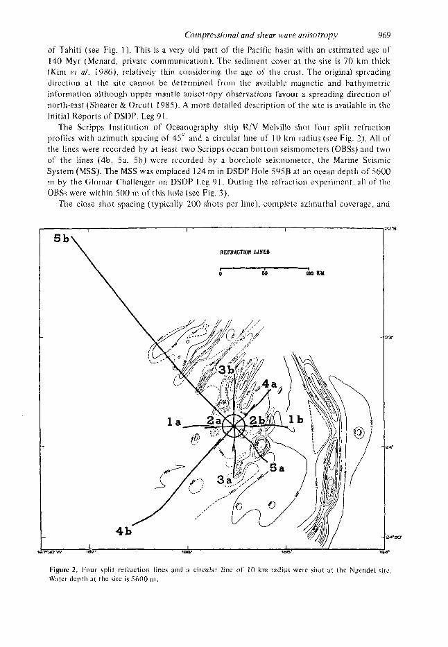
The Scripps Institution of Oceanography ship R/V Melville shot foui- split refraction profiles with azimuth spacing of 45" and a circular line of 10 kni radius (see Fig. 2) . All of the lines were recorded by at least two Scripps ocean bottom seismometers (OBSs) and two of the lines (4b, 5a. 5b) were recorded by a borehole seisniometer, the Marine Seismic System (MSS). The MSS was emplaced I24 m in DSDP Hole S9SB at an ocean depth of 5600 m by the Clomar Challenger on DSDP Leg 91 . During the refraction experiment. all of the OBSs were within 500 m o f this hole (see Fig. 3).

The close shot spacing (typically 200 shots per line), complete azimuthal coverage, and

r I I

Figure 2. ]:our split refraction lines and B circular line of 10 k m radius were shot a t the Npcndei site. Water dcpth a t t he site is 5600 i n .

Y70 I? M. Shearer arid J. A . Orcxtt

OBS Locations

-23.8 1 E

t

I I I 0 0.5 km

Karen

@Sury

+ Borehole

-23.825 I -165.535 - 165.5

Figure 3. 95 p e r cc t l r confitlcncc l imits f o r t l i c 013s locations. :\I1 OI3Ss wcre within S O 0 111 of the bore- hole.

multiple receivers conibine to iiiake this perhaps the largest seismic refraction data set yet collected at a single site. The four channel OBSs recorded about 8000 individual seismo- grams; the MSS recorded an additional 600 seismograms. Procedures used to process these data (calculate shot ranges, make topographic corrections. etc.) are described for both the OBS and MSS data sets in the Initial Reports of DSDP. Leg 91 (Shearer et al. 1986a; Whitniarch ct a / . 1086). These papers also show record sections for each seismic line and receiver.

A previous paper (Shearer & Orcutt 1985) examined P-wave travel titnes from these data and found evidence for anistropy both within the upper mantle and in the upper crust. The fast direction in the upper mantle is about N3OoE, approximately orthogonal to the fast crustal direction. This paper is a continuation o f this work and extends the analysis to include synthetic seismograni modelling of both the P- and S-wave velocity structure a t the Ngentlei site.

Upper crustal P-wave velocity structure

The P-wave velocity structure of the uppei- crust has i ts greatest influence on seismic arrivals a t ranges out to about 20 km. The Ngendei OBS data. while noisier than the MSS data (Adair, Orcutt & Jordan 198G), are more complete than those of the MSS and thus better suited for upper crustal P-wave analysis. We thus used only the OBS data at nearby ranges (0--10 kin), rescrving the MSS data for inore distant ranges (20---I 00 km) where the

Corupressiotiul atid shcar wave atiisotropy 97 I

advantage of lower noise levels becomes more important than the disadvantage of. t h e sparse azimuthal coverage of the MSS. A previous analysis oiP-wave travel times for the 013s data a t nearby ranges led t o a preliminary P-wave velociiy structure wliicli included a~imut l i s l differences in velocity related t o upper crustal anistropy ;it the Ngendei site (Shearer 22 Orcutt 1985). This analysis did not use any of the amplitude or waveform content of the

4. i 1 I

L 3.81 :, , , , I 5 10 15 20 3.70

501 401

301

4 5 110 1'5 22 Ranye ( k r n )

,- I , , , , I 5 10 15 21) 3. i0

~ ~ n e 4a 4. 1 1 - 1

!

i / I

3.7: 5 1 1 0 I5 20

4LJ 50i

Range (krn)

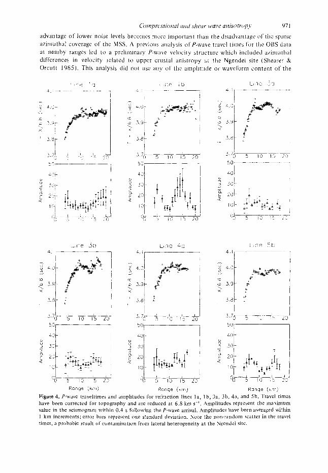
Figure 4. P-wave traveltimes and amplitudes for refraction lines l a , I b , 32, 3b, 43, and 5b. Travel times have been corrected for topography and are reduced at 6.8 km s- ' . Amplitudes represent the masimum value in the seismogram within 0.4 s following the P-wave arrival. Amplitudes have been averaged within 1 km increments; error bars represent one standard deviation. Note the non-randon) scatter in the travel times, a probable result of contamination from lateral heterogeneity a t the Ngcndei site.

972

data , information employed in this paper in synthetic seismogram modelling to better, constrain the velocity structure.

As a first step in this modelling procedure, we reduced each seismogram t o just two numbers, the P-wave traveltime and amplitude. The P-wave travel times were picked by hand using an interactive picking program. Amplitudes were determined by finding the maximum value in a 0.4 s window following the P-wave pick. The 0.4 s window was chosen t o be long enough to include the first bubble pulse (usually the largest amplitude in the P-wave) but short enougli t o exclude the P,,P arrivals of the Moho triplication.

P-wave amplitudes tend t o scatter widely within individual refraction lines, probably due to lateral heterogeneities causing focusing and defocusing of seismic energy. Source irregularities were ininimized for the shots at these nearby ranges by suspending the shots from balloons so that they exploded at a constant depth of 10 m. In order to remove the gross scatter in the amplitude data we averaged amplitudes within 1 kin sections for each refraction line. For a typical line, each 1 kni section contained about six P-wave arrivals (three shots per km and two OBS receivers). Fig. 4 shows P-wave travel times and amplitudes (including one standard deviation error bars) for refraction lines la , l b , 3a, 3b, 4a, and 5b. Travel times have been reduced at 6.8 km s-' and amplitudes have been scaled for range and shot weight by the empirical formula

P. M. Shearer and J. A . Orcutt

2 0 . 6 5

A ={;} {:} A, , , ,

where

Y = range

w = shot weight.

Although topographic corrections can remove the gross effects o f bathymetric differences on P-wave travel times, such corrected travel times tend to exhibit more scatter in regions containing significant seafloor topography (Shearer et al. 1986a). Not surprisingly, we noticed similar increased scatter in the observed P-wave amplitudes for shots near the sea- mounts and ridges at the Ngendei site. Fig. S shows P-wave arrival times and amplitudes compared t o the ocean depth along refraction lines 4b and 5a. Both the travel times and amplitudes show significant anomalies related to the irregularities in the sea floor. P-wave travel times are reduced for shots above topographic highs (although note the slight range offset), reflecting the decreased travel time in the relatively slow ocean. Amplitude behaviour is less predictable but certainly exhibits more scatter in these lines than in the lines shown in Fig. 4 , which were along relatively smooth parts of the sea floor.

Because of these large topographic effects, our analysis excluded data from those lines which contained significant sea floor relief. The lines shown in Fig. 4 all contain less than 1 SO in of relief a t the ranges shown, although it was necessary t o truncate line 3b at 18 km, line 4a a t 17 km, and line Sb a t 18 k m in order to meet this criterion. To account for the slight remaining variations in water depth, topographic corrections based on the ray path through the water were applied (Shearer et al. 1986a, for a full discussion). We did not use lines 2a and 2b in our amplitude analysis because those lines used larger shots which cannot be easily compared t o the shots used in the other lines, and also because 2a and 2b duplicate data already available from lines l a and I b (see Fig. 2).

Although there are significant variations between the range versus amplitude behaviour of the different refraction lines shown in Fig. 4, some gross trends are apparent. Amplitudes tend to increase rapidly from very small d u e s at 3 kin t o an amplitude peak at about 5 or

Compressional and shear wave anisotropy 973

i ~ n e 5a

3'80 3.gi 5 10 15 20

$ 4. I

> ; 4.0,

' 3.9

LL "% 5 10 15 20

4.5

v

5 2 5.5

n 0

6'o0 5 10 15 20 6'o0 5 10 15 20 Range (km) t?onge (km)

Figure 5. P-wave travel times and amplitudes for refraction lines 4b and 5a, compared to bathymetry. Topographic perturbations have a strong effect on both travel times and amplitudes.

6 km, then decrease to a local minimum at about 10 km. Some of the lines contain another amplitude peak a t about 15 km but this is highly variable between lines. The P-wave travel times for these lines show an azimuthal variation which indicates that upper crustal P-wave velocities are faster in the direction N12O0E and slower in the direction N30"E (Shearer & Orcutt 1985). Because of this systematic difference in P-wave travel times, which we believe is caused by anisotropy in the upper crust, we divided the data into what we will call the NNE lines (lines 3a, 3b , and 4a) and the ESE lines (lines la , l b , and 5b). Fortunately, this division based on traveltime differences also appears to make sense in terms of the P-wave amplitudes. The amplitude peak at about 15 km is more prominent in the ESE lines than in the NNE lines.

Although such a division of the data set into two orthogonal azimuths is necessarily approximate (individual lines are 15 t o 30" off from the group azimuth) i t has the advantage of allowing us t o compute separate average velocity versus depth profiles for the fast crustal direction (ESE) and the slow crustal direction (NNE). Since the crustal anisotropy appears t o exhibit a 28 variation of velocity with azimuth (Shearer & Orcutt 1985) this will be

974

sufficient t o define the azimuthal P-wave velocity anisotropy. The averaging of adjacent azimuths will simply have the effect of slightly underestimating the total magnitude of the anisotropy a t a given depth.

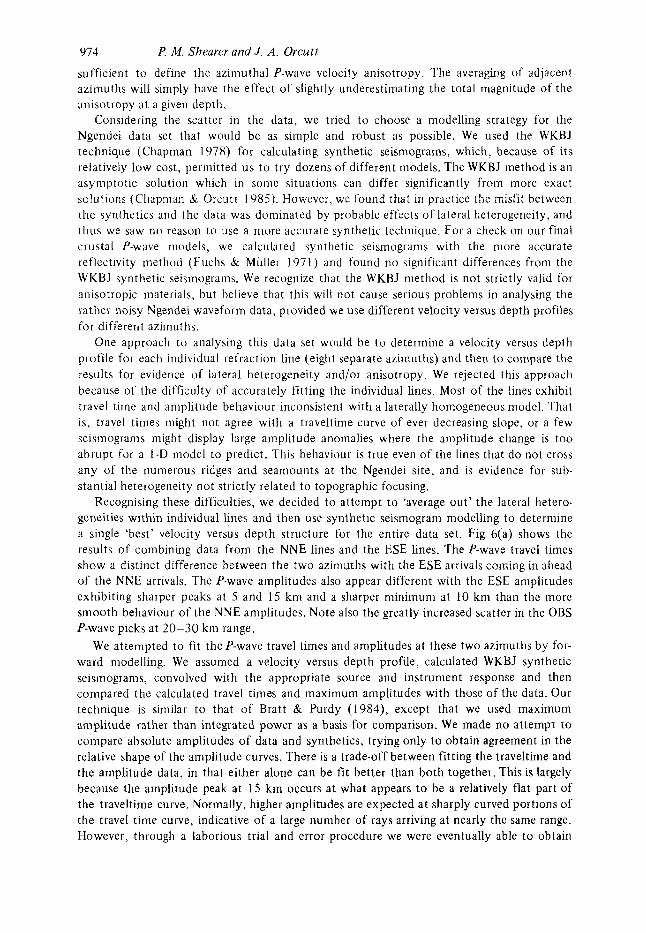
Considering the scatter in the data, we tried to choose a modelling strategy for the Ngendei data set that would be as simple and robust as possible. We used the WKBJ technique (Chapman 1978) for calculating synthetic seismograms, which, because of its relatively low cost, permitted us t o try dozens of different models. The WKBJ method is an asymptotic solution which in some situations can differ significantly from more exact solutions (Chapman di Orcutt 19853. However, we found that in practice the misfit between the synthetics and the data was dominated by probable effects of lateral heterogeneity, and thus we saw no reason to use a more accurate synthetic technique. For a check on our final crustal P-wave models, we calculated synthetic seismograms with the more accurate retlectivity method (Euchs & Muller 1971) and found no significant differences from the WKBJ synthetic seismograms. We recognize that the WKBJ method is not strictly valid for anisotropic materials, but believe that this will not cause serious problems in analysing the rather noisy Ngendei waveform data, provided we use different velocity versus depth profiles for different azimuths.

One approach to analysing this data set would be to determine a velocity versus depth profile for each individual refraction line (eight separate azimuths) and then t o compare the results for evidence of lateral heterogeneity and/or anisotropy. We rejected this approach because of the difficulty of accurately fitting the individual lines. Most of the lines exhibit travel time and amplitude behaviour inconsistent with a laterally homogeneous model. That is, travel times might not agree with a traveltime curve of ever decreasing slope, or a few seismograms might display large amplitude anomalies where the amplitude change is too abrupt for a I -D model to predict. This behaviour is true even of the lines that do not cross any of the numerous ridges and seamounts a t the Ngendei site, and is evidence for sub- stantial heterogeneity not strictly related t o topographic focusing.

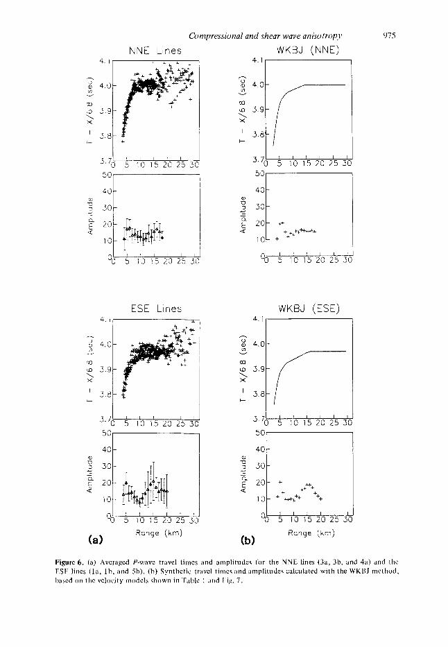
Recognising these difficulties, we decided to attempt t o ‘average out’ the lateral hetero- geneities within individual lines and then use synthetic seismogram modelling t o determine a single ‘best’ velocity versus depth structure for the entire data set. Fig 6(a) shows the results of combining data from the NNE lines and the ESE lines. The P-wave travel times show a distinct difference between the two azimuths with the ESE arrivals coming in ahead of the NNE arrivals. The P-wave amplitudes also appear different with the ESE amplitudes exhibiting sharper peaks at 5 and 15 km and a sharper minimum at 10 km than the more smooth behaviour of the NNE amplitudes. Note also the greatly increased scatter in the OBS P-wave picks a t 20-30 km range.

We attempted t o fit the P-wave travel times and amplitudes at these two azimuths by for- ward modelling. We assumed a velocity versus depth profile, calculated WKBJ synthetic seismograms, convolved with the appropriate source and instrument response and then compared the calculated travel times and maximum amplitudes with those of the data. Our technique is similar t o that of Bratt & h r d y (1984), except that we used maximum amplitude rather than integrated power as a basis for comparison. We made no attempt t o compare absolute amplitudes of data and synthetics, trying only t o obtain agreement in the relative shape of the amplitude curves. There is a trade-off between fitting the traveltime and the amplitude data, in that either alone can be fit better than both together. This is largely because the amplitude peak at 15 km occurs a t what appears t o be a relatively flat part of the traveltime curve. Normally, higher amplitudes are expected a t sharply curved portions of the travel time curve, indicative of a large number of rays arriving at nearly the same range. However, through a laborious trial and error procedure we were eventually able to obtain

P. M. Shearer and J. A. Orcutt

Compressional and shear wave anisotropy 975

NNE Lines 4. I

,--. h: 4.0 Y

m 9 3.9 >

'.'O 5 10 15 20 25 30

3 3 30 I

5 1'0 1'5 ;I) 215 3

ESE Lines 4. I ( +

- 3.70 5 10 15 20 25 31

40

4 5 110 115 210 215 312 Range (krn)

(a)

WKBJ (NNE) 4r----7

5017----- 40

d - '0 5 10 15 20 25 3

WKBJ (ESE)

4.0

cn

u 3'70 5 10 15 20 25 3

40

(b)

h ' 0 5 10 15 20 25 3C

Range (krn)

Figure 6. (a) Averaged P-wave travel times and amplitudes for the NNE lines (3a, 3b, and 4a) and the ESE lines ( l a , l b , and 5b). (b) Synthetic travel times and amplitudes calculated with the WKHJ method, based on the velocity models shown in Table 1 and l ,ig. 7.

P. M. Shearer and J . A . Orcurt

Ngendei Velocity Model 976

0

- 2 E r: W

C . -

5 6 a Q a

1

S-waves

P - waves

8

3 4 5 6 7 8 Velocity (km/sec)

Figure 7. Anisotropic velocity versus depth model which satisfies the Ngendei data. The solid line is the “ I < velocity model; the dashed line is the 1 S I ; model.

Table 1. Ngendei P-wave and S-wave velocity versus depth model for NNE and ESE azimuths. Equivalent Poisson’s ratio u is alw shown.

Depth NNE arimuth ESE azimuth Comments

Ocean C m t P S U P 5 U

km km km/s km/s km/s km/s

0.0 - 5.65 1.52 - 5.58 -0.07 1.52 - 5.58 -0.07 1.6 0.12 .50 1.6 0.12 .50 sediment surface 5.65 0.0 1.6 0.12 .50 1.6 0.12 .so 5.65 0.0 4.22 2.33 2 8 4.38 2.42 .2a crustal surface 5.704 0.054 4.32 2.38 .2a 4.49 2.47 .2a MSS depth 6.50 0.85 5.85 3.15 .30 6.11 3.24 .30 6.66 1.015 6.16 3.30 .30 6.29 3.34 .30 6.90 1.25 6.41 3.44 .30 6.55 3.48 .30 7.05 1.40 6.57 3.52 .30 6.57 3.52 .30 7.36 1.71 6.64 3.75 .27 6.64 3.75 .27 7.67 2.02 6.80 3.75 2 8 6.80 3.75 .28

ocean surface OBS depth

- 1.52 - 1.52 -

-

- -

12.00 6.35 6.80 3.75 .28 6.80 3.75 .28 Moho 12.35 6.70 8.40 4.65 .28 7.95 4.65 .24 20.00 14.35 8.45 4.75 .27 8.15 4.85 .23

Compressional and shear wave anisotropy 977

velocity versus dcptli profiles which fit both the traveltime and amplitude data reasonably well.

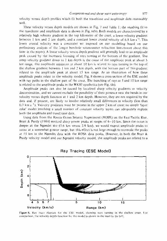
These velocity versus depth models are shown in Fig. 7 and Table I : the resulting fit to the traveltime and amplitude data is shown in Fig. 6(b). Both models are characterized by a relatively high velocity gradient in the top kilometre of the crust, a lower velocity gradient between 1 km and 2 kni depth, and a constant lower crustal velocity of 6.8 km s-I. This lower crustal velocity was a constraint we imposed on our modelling based on our preliminary analysis o f the longer borehole seismonieter 1-efraction lines (more about this later in the paper). A linear velocity versus depth gradient will generally lead t o an amplitude peak caused by the increased focusing of rays turning at the bottoni of the gradient. The steep velocity gradient down to I km depth is the cause of the amplitude peak at about 5 km range. The amplitude tninimum at aboul 10 kni is related to rays turning in the top of the shallow gradient between I kin and 2 km depth, with the bottoni part of this gradient related to the amplitude peak at about 15 kin range. As a n illustration of how these amplitude peaks relate to the velocity model, Fig. 8 shows a cross-section of the ESE model with ray paths in the shallow part of the crust. The bunching of rays at 5 and 15 kin range is related to the amplitude peaks in the WKHJ synthetics (see Fig. 6b).

Amplitude peaks can also be caused by localized sharp velocity gradients or velocity discontinuities, and we cannot exclude tlie possibility of their presence near the bends in o u r velocity versus depth function at 1 and 2 km depth. However, they are not required by the data and, if present, are likely to involve relatively srnall differences in velocity (less than 0.3 kni s-’) . Velocity gradients must be present in the upper 2 kni of crust; no simple ‘layer cake’ rriodel involving a small number of constant velocity layers can adequateiy explain both the amplitude and travel time data.

Using data from the Rivera Ocean Seismic Experiment (ROSE) on the East Pacific Rise, Bratt & Purdy ( 1 984) noticed sharp power peaks at ranges of 6-1 0 km. Since the ocean is deeper a t the Ngendei site (5.6 km versus 2.9 km), we would expect amplitude peaks to occur at a somewhat greater range, but this effect is not large enough to reconcile tlie peaks a t 15 km in tlie Ngendei data with the ROSE data peaks. However, in both the Bratt & Purdy velocity model and our Ngendei velocity model. the amplitude peaks are related t o a

h

E Y v

Ray Tracing (ESE Model) 0

2

4

6

8

4 5 6 7 5 10 15 Velocity (km/s) Range (km)

Figure 8. Ray trace diagram f o r the I.:SI.. modcl, showing rays turning in thc shallow crust . I o r comparison. tlic velocity dep th function f o r the model is shown in ttic inset to the Ictt.

Y78

velocity gradient near the bottom of layer 2, and thus we believe that they are caused by similar structures. The difference in the position of the peaks results from overall differences in the velocity models, in particular from the much slower upper crustal velocities a t the younger ROSE site. Bratt & Purdy related the range variations in their observed peak positions to differences in layer 2 thickness: our observed amplitude peaks exhibit a similar range variation (see Fig. 4) and support this conclusion. The Ngendei and ROSE data sets are also similar in that some lines d o not show strong amplitude peaks.

P-wave anisotropy in the top 1 ---1.5 km of the crust a t the Ngendei site is indicated by the approximate 0.2 km s - ' offset between the NNE and ESE velocity profiles. The traveltime data alone indicate that ESE velocities must be faster than NNE velocities in the upper crust (Shearer & Orcutt 1985). However, the amplitude information which we are now considering give us much better constraints on the depth and magnitude of this velocity difference. In particular. wc believe tha t P-wave anisotropy is confined to the top 1-1 5 km of the crust, and that i t is probably present at the surface of the crust. The overall similarity of the N N E and ESE amplitude versus range curves indicates that there can be no large differences in the shape of the velocity profiles. The slower near surface velocities for our NNE model are consistent with the broad nature of the data amplitude peak at 5 km range. Differences in the transition a t 1-1.5 km depth from the higher t o the lower velocity gradient lessen the severity of both the amplitude minimum at 10 km and the amplitude peak at 15 kni for the NNE model.

The resolution of our model is difficult to assess quantitatively, particularly because we have attempted t o produce a model which in some sense averages the differences between individual refraction lines related to lateral heterogeneities. I t is interesting t o note that the amplitude peak near 15 kin range js generally sharper for the individual lines (Fig. 4) than on the azimuthally averaged lines (Fig. 6a). This is because the range a t which the amplitude peak occurs varies between the lines so that the averaged peak becomes shortened and broadened. This suggests that the transition to the constant velocity layer a t 2 km depth may be sharper (causing a higher, narrower amplitude peak) than in our model but that the

P. M , Shcurer arid J. A . Orcutt

Ngendei Line 5b

6 8 10 1 2 1 4 IF 18 Ran3e ( k m )

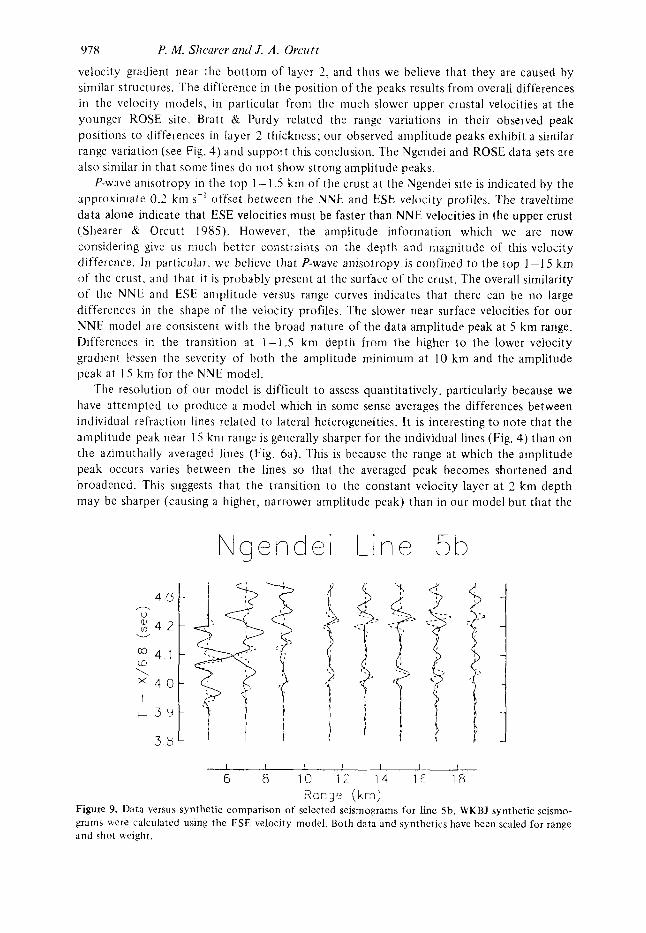
Figure 9. Data versus synthetic comparison of selected seismograms for line 5b. WKBJ synthetic seismo- grams were calculated using the LSE velocity model. Both data and synthetics have been scaled for range and s h o t weight.

Conipressiorial and shear wave anisotropy 979

depth t o this transition may vary between lines (changing the range at which the peak occurs). If this is the case. our model is still approximately correct for a laterally averaged earth since averaging different velocity profiles would have a similar effect.

As a final check, we compared synthetic seismograms to data for line 5b, using the ESIi velocity model. Fig. 9 shows a comparison o f selected seismograms, scaled for range and shot weight, Although this model is an average for all lines of similar azimuth, the fit to line 5b is still reasonably good. In particular, note the reproduction of the large amplitudes at ranges of 6 and 16 kni. The two distinct pulses in the data and synthetics are the initial source and first bubble pulses, often not separated with less broadband instruments than the Scripps OBS.

P-wave velocity structure near the Moho

At ranges greater than 20 km, noise severely limited the quality of the OBS data. Much o f this noise was associated with operations of the drilling ship, the Glomar Challengei-. during the refraction shooting. However. even under quiet conditions OBS noise levels were about 10 to 15 d b higher than MSS (borehole) noise levels (Adair et al. 1986). Since signal levels as recorded by the OBSs and the MSS were approximately the same (Shearer er al. 1986b) this resulted in a considerable signal-to-noise improvement for the MSS recordings. This proved particularly important for examining the relatively weak P,, arrivals at the Ngendei site. P, arrivals on the OBS seismograms could only be picked out to ranges of about SO km. Although these picks proved adequate to constrain the direction and magnitude of upper mantle anisotropy at the Ngendei site (Shearer & Orcutt 1985) the poor quality of the P,, arrivals precluded the possibility of any amplitude or waveform analysis.

Thus, we decided t o use only MSS data from the two orthogonal lines 4b and Sb (see Fig. 2) for modelling with synthetic seismograms. Fortunately, these lines are approxiinately aligned with the fast and slow axes of the upper mantle anisotropy, so the lack of complete azimuthal coverage is not a severe problem. OBS P-wave traveltime data from all azimuths indicate that lower crustal velocities do not vary with azimuth and that the upper mantle anisotropy can be described with a simple 20 function of azimuth (,Shearer & Orcutt 1985). We assumed the upper crustal P-wave model discussed in the previous section for all subsequent modelling,

Fig. 10 shows MSS record sections for lines 4 b and 5b and our best fitting WKBJ P-wave models, based on the velocity models shown in Fig. 7. Both data and synthetics have been reduced at 8 km s-' and scaled for range and shot weight. Topographic time corrections have been made to account for differences in sea floor bathymetry along the lines in a similar way t o the OBS corrections discussed earlier; however times and ranges have not been corrected t o the sea floor. The data have been multiplied in the frequency domain with a sinc4 function in order to make a direct comparison with the WKBJ synthetics, which have undergone a similar smoothing operation (Chapman & Orcutt 1985). Alternatively, the WKBJ synthetics could have been calculated a t a much higher sampling rate than the data, but this seemed unnecessary considering the generally low frequency nature of the MSS data which are little affected by the smoothing operation. We checked our final models by calculating synthetic seismograms with the reflectivity method (Fuchs & Muller 197 I ), and found n o significant differences from the WKBJ results.

The most striking difference between the lines is in the P, arrivals, which for line 4 b are both weaker and faster than those of line 5b. Our synthetic seismogram modelling suggests that the upper mantle P-wave velocity in the direction of line 4b is 8.4 km s-' with a relatively weak velocity gradient of 0.007 (km s-' ) km-' compared to a velocity of 7.95

8 -

7 - U al In v

p- I

t- 5 -

4 -

P. M. Shearer wid J. A . Orcutt

Line 4b (MSS)

I I I 1 1

20 4 0 60 80 100 Range (km)

Line 5b (MSS)

I 1 I 1 I

20 40 60 80 100 Range (krn)

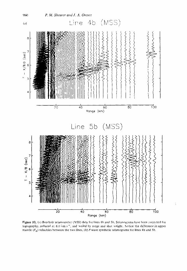
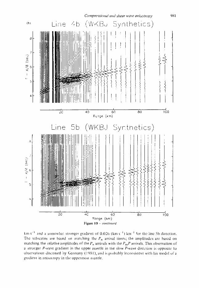
Figure 10. (a) Boreliole seisrnonieter (MSS) data for lines 4b and 5b. Seismograms have been corrected for topography, reduced at 8.0 km s-', and scaled by range and shot weight. Notice the difference in upper mantle ( P , ) velocities between the two lines. (b) P-wave synthetic seismograms for lines 4b and 5b.

Compressional and shear wave anisotropy 981

Line 4b (WKBJ Synthet ics)

c

1 I I I I

20 40 60 80 100 Range (krn)

Line 5b (WKBJ Synthet ics)

I I I I

20 50 60 80 100 Range (krn)

Figure 10 ~ confir?ued

kin s - ' and a soniewhat stronger gradient o f O.O?(> ( k m s C ' ) kni..' for the line Sb direction. 'The velocities are based on matching the P, arrival t imes; the amplitudes are based on matching the relative amplitudes o f the P, arrivals with the P,P arrivals. This observation o f a stronger P-wave gradient in the upper marttie in the slow P-wave directioii is opposite to observalioris discussed by Garinany ( 1 981), and is pi-obably inconsistent with his model of a g radkn l in anisotropy in the uppermost Iiiantle.

982 P. M. Shearer and J. A . Orcuti

The large velocity increase at the Moho in the model for line 4b is required by the significant P,,P reflections at large ranges, the low amplitude of the P, arrivals compared to P,P, and the observed phase velocity of the mantle arrivals. The smaller jump in velocity for the model corresponding to line 5b serves t o increase the size of P, and concentrates the larger P,P amplitudes closer t o the near caustic. Note in Fig. 1 q b ) that the ratio of P, t o P,P amplitudes is substantially smaller for the line 5b synthetics than for the 4 b synthetics. The weak crustal P-waves at ranges of 20-30 kni are indicative of a very low velocity gradient in the lower crust. For both lines we found that a constant lower crustal velocity of 6.8 kin s-' provided the best fit to the position and amplitude of the crustal P phase.

Significant differences remain between the synthetic record sections and the data. For example. the line 4 b data contain an amplitude peak on the retrograde P,P branch at 40GSO km range. The amplitude peak in the synthetics is a t a closer range of 20-40 km and is associated with the caustic a t the end of the retrogt-ade branch. After much adjusting of our models we came t o realize that no 1-D model can explain the line 4b data, since for such models large amplitudes cannot occur in the middle of retrograde branches, only near the endpoints. An additional problem is that P,P amplitudes at long ranges are much greater in the line 4b data than in the line Sb data, a difference which cannot easily be accounted for in the synthetics. Thus, we believe that any fit to the data which does not include lateral heterogeneity will only be approximate. In particular, it seems likely that undulations in the Moho surface are distorting the amplitude behaviour of the P,P branch.

The P-wave velocity model we are now proposing for the Ngendei site differs from that which we proposed earlier based only upon P-wave travel times (Shearer & Orcutt 1985). The earlier model included a substantial velocity gradient throughout layer 3. The amplitude data which we have discussed preclude such a high gradient, and our new model with a constant-velocity layer 3 still fits the crustal P-wave travel times quite well. The crustal P-wave anisotropy i n the earlier model is large in magnitude (0.4 km s-' difference between azimuths) and is confined to a layer between 0.75 and 1.4 km depth. We now believe that the anisotropy is smaller in magnitude (= 0.2 km s-') and is present throughout the top 1.4 km of crust. P-wave travel times alone cannot distinguish between these two models; there is a trade-off between the magnitude of the anisotropy and the thickness of the anisotropic layer. However, the P-wave amplitude data are inconsistent with the sharp velocity discontinuities of the earlier model, and thus favour the smoother velocity profiles of the new model.

Upper crustal S-wave velocity structure

The quality of the shear waves observed in the Ngendei refraction lines is highly variable. Many of the lines have well defined shear wave arrivals, while in other lines shear waves are not observed. However, enough data are present to form constraints on the shear wave structure a t the Ngendei site. As in the case of the P-wave analysis, we decided to use the OBS data t o examine upper crustal 5'-wave structure, reserving the MSS data at longer ranges for the lower crustal and upper mantle structure.

Using interactive picking software, we picked shear wave arrivals at ranges out to 20 km. T w o shear wave arrivals could usually be identified. Arriving first was the wave which con- verted to a P-wave at the crust-sediment interface. This arrival was most prominent on the OBS vertical component. Arriving about 0.55 s later was the direct S-wave through the sediments, which appeared most prominently on the OBS horizontal channels. Since we know that the sediments are 70 ni thick with a P-wave velocity of about 1.6 km s-', this allowed us to calculate a sediment shear wave velocity o f about 120 m s-'. This value is in

Compressional and shear wave anisotropy 983

agreement with that obtained by modelling eigenfrequencies associated with sediment reverberations in Ngendei earthquake data (Sereno & Orcutt 1985).

Since many of the shear wave arrivals were very weak and contaminated by noise from the earlier arriving P-waves. i t was difficult to accurately pick the travel times. In particular, picking traces individually without reference t o those at similar ranges along the same line proved impossible. However, by displaying an entire reduced record section on the computer screen a t once, and switching between the horizontal and vertical channels, it often became possible to identify phases which otherwise would be missed. In this way, 41 5 shear wave arrivals were identified. including at least some for all lines except lines 4b and 5a.

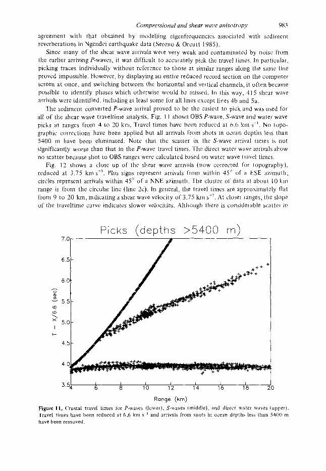
The sediment converted P-wave arrival proved t o be the easiest to pick and was used for all of the shear wave traveltime analysis. Fig. 1 1 shows OBS P-wave, S-wave and water wave picks at ranges froin 4 to 20 kin. Travel times have been reduced at 6.6 kin s-I. No topo- graphic corrections have been applied but all arrivals from shots in ocean depths less than 5400 ni have been eliminated. Note that the scatter in the S-wave arrival times is not significantly worse than that in the P-wave travel times. The direct water wave arrivals show no scatter because shot to OBS ranges were calculated based on water wave travel times.

Fig. 12 shows a close up of the shear wave arrivals (now corrected for topography), reduced at 3.75 kin s-I. Plus signs represent arrivals from within 45" of a ESE azirnutli; circles represent arrivals within 45" of a NNE azimuth. The cluster of data a t about 10 kin range is from the circular line (line 2c). In general, the travel times are approximately flat from 9 t o 20 k m , indicating a shear wave velocity of 3.75 km s-'. At closer ranges, the slope of the traveltime curve indicates slower velocities. Although there is considerable scatter in

T t . - I I I I I 1 I 6 8 10 12 14 16 18

Range (krn)

I

Figure 11. Crustal travel times for P-waves (lower). S-waves (middle), and direct water waves (upper). Travel times have been reduced at 6.6 km s- ' and arrivals from shots in ocean depths less than 5400 ni have been removed.

984 P. M. Shearer arid J. A . Orcutt

Picks (depths >5400 m>

+

0

Range (km)

0

Figure 12. Close-up of S-wave arrivals, reduccd a t 3.75 k m s I'lus signs arc arrivals from within 45" o f a CS1: azimuth; circles represent arrivals within 45" of a NNI : azimuth. S-ivave travel times have been corrected for topographic variations.

the data, the ESE arrivals come in slightly before the NNE arrivals a t ranges from 6 to 1 I km. Beyond 11 kni, the arrivals appear randomly scattered with respect t o azimuth.

This pattern is similar to that which can be seen with greater clarity in the P-wave travel- time data (Shearer & Orcutt 1985). The azimuthal S-wave travel time difference seems clearest at ranges between 0 and 1 I kin. Since the slope of the traveltinie curve is approxi- mately flat at these ranges, the data can be reduced for a constant velocity in order t o make a traveltime versus azimuth plot. Fig. 13 shows such a plot for S-wave traveltime picks between 9 and 11 k m , reduced at 3.75 km s-'. Topographic time and range,corrections have adjusted the arrivals t o the sea floor. The vertical alignments in the plot represent individual refraciion lines, which were shot a t approximately constant azimuth. Points between these aligiimetits represent data from the circular line. The data show considerable scatter, presumably representing lateral heterogeneities. However, some systematic azimuthal trends are apparent. Arrivals a t azimuths of 0-45" (NNE) and 180&325" (SSW) are generally late, while arrivals a t azimuths of 90-135" (ESE) and 270--3 I5" (WNW) are generally early.

The crustal shear wave phase relevant to these picks is vertically polarized since only SV waves would convert to P-waves in the sediment. Following Backus (I 965) and Crampin (1 977) we may express the velocity of a quasi-SV wave (approximately vertically polarized) travelling within a horizontal plane in a generally weakly anisotropic medium as

V* = a , + a2 cos 20 + u 3 sin LO

0 80

0 15 n 0

E 070 W

s, I' r) 0 65 \ X

I + 060

0 55

0 50

Cornpressiotial and shear wave anisotropy 985

Ngendei S-waves (9 - 1 1 km)

0

0

0 0

0 0

0

0

0 0

0 0 0

0 O 0 0

0 I I I I I

0 90 180 270 360 Shot az lmuth (deg)

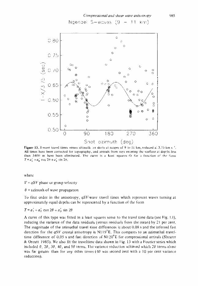
Figure 13. S-wave travel times versus azimuth tor shots a t ranpes of 9 to 1 1 km. reduced a t 3.75 km s '. All times have been corrected f o r topography, and arrivals from rays entering the seatloor a t depths less than 5400 m have been eliminated. The curve is il least squares fit for a function o f the form T = a ; +a; c o s 2 0 + a ; s in2r) .

where

Y = 4SV phase or group velocity

0 = azimuth of wave propagation

To first order in the anisotropy, qSV-wave travel times which represent waves turning at approximately equal depths can be represented by a function of the form

T = u i +a ; cos 28 + a ; sin 28

A curve of this type was fitted in a least squares sense to the travel time data (see Fig. 13), reducing the variance of the data residuals (versus residuals from the mean) by 2 1 per cent. The magnitude of the azimuthal travel time differences is about 0.08 s and the inferred fast direction for the 4SV crustal anisotropy is N1 19'E. This compares to an azimuthal travel- time difference of 0.05 s and fast direction of N120'E for compressional arrivals (Shearer & Orcutt 1985). We also fit the traveltime data shown in Fig. 13 with a Fourier series which included 0, 2 0 , 30, 40, and 50 terms. The variance reduction achieved which 28 terms alone was far greater than for any other terms (40 was second best with a 10 per cent variance reduction ).

986 P. M. Shearer and J. A . Orcutt We obtained these results by applying topographic time and range corrections for both

P- and S-waves. These corrections are based on finding the intersection of the ray path with the appropriate point on the sea floor. The P-wave topographic corrections are described in detail in Shearer er a/. (1986a). We determined the S-wave corrections in a similar manner, except that we used a constant phase velocity of 3.75 km sC1 in calculating the water path and did not apply a dt/dh correction. Although all data discussed in this paper have been corrected for topography, we wish t o emphasize that our results are not very sensitive t o these corrections. Even if‘ we had applied no corrections at all, we would have obtained similar results regarding the orientation and magnitude of anisotropy.

The similarity of the azimuthal pattern of the Ngendei S-wave travel times to the P-wave pattern is not additional evidence for anisotropy at the Ngendei site since the leading alternative (non-anisotropic) explanation for the observed azimuthal variations in travel times is lateral heterogeneity. A hypothetical slow ‘blob’ of crust would slow both P- and S-waves and lead to similar traveltime patterns. Thus, it is not surprising that we observe an azimuthal dependence of S-wave travel times. However, we believe that anisotropy is a more likely explanation for the gross azimuthal trends in the data, since we would not a priori expect lateral heterogeneity to be organized in a 28 sense. Furthermore, if we accept that these traveltime patterns are caused by anisotropy, then the shear wave data place additional constraints on the anisotropic elastic constants in the upper crust. We will discuss these constraints in more detail later in this paper.

The noisy and irregular nature of the S-wave arrivals precluded any amplitude or wave- form analysis of the data. In addition,S-wave amplitudes are at least partially dependent on P S conversion efficiency, which depends on properties a t the sediment/basement interface and not on the velocity structure a t depth. Thus, we formulated velocity versus depth models based only on the S-wave travel times. Fig. 7 illustrates a simple S-wave velocity profile of the upper crust which is consistent with the travel time data, although more complicated models are certainly not excluded. The P- and S-wave velocity models are generally consistent but with the difference that the S-wave profile reaches the constant layer 3 velocities a t about 1.7 km depth versus 2 km for the P-wave velocity profile. This difference appears required by the traveltime data and produces a slight dip in the Poisson’s ratio of the model at a depth of 1.7 km in the crust. Spudich and Orcutt made a similar observation in synthetic modelling of refraction data in the eastern Pacific (Spudich bi Orcutt I 9XOa) .

S-wave velocity structure near the Moho

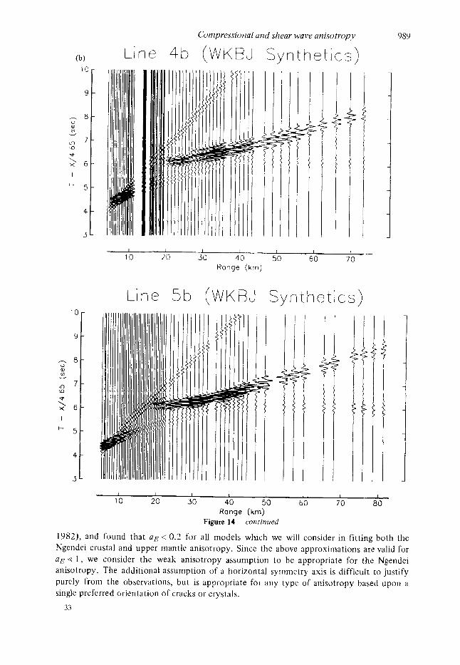
As in our P-wave analysis, we used MSS data from the two orthogonal lines 4b and 5b (see Fig. 2) a t ranges of 20 to 100 km in order to constrain the shear wave structure of the lower crust and upper mantle. Fig. 14 shows MSS vertical component record sections for lines 4 b and 5b and our best fitting WKBJ S-wave models, based on the velocity model shown in Fig. 7 and Table 1. Both data and synthetics have been reduced at 4.65 km sC1 and scaled for range and shot weight. Topographic time corrections appropriate for S-wave phase velocities have been made t o account for differences in sea floor bathymetry along the lines; however, times and ranges have not been corrected to the sea floor. The data have been multiplied in the frequency domain with a sinc4 function in order t o make a direct comparison with the WKBJ synthetics.

A very weak S, arrival is apparent in these record sections with an apparent phase velocity of about 4.65 kin s-l in both lines. S , observations are rare in seismic refraction experiments; our success here was due in part to the low noise levels of the MSS borehole

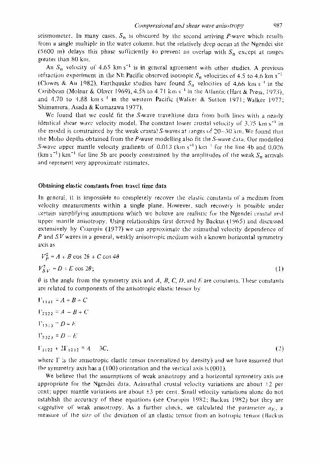
Compressional atzd shear wave anisotropv 987

seismometer. In many cases, S, is obscured by the second arriving P-wave which results from a single multiple in the water column, but the relatively deep ocean at the Ngendei site (5600 m) delays this phase sufficiently t o prevent an overlap with S , except a t ranges greater than 80 kin.

An S, velocity of 4.65 km s-' is in general agreement with other studies. A previous refraction experiment in the NE Pacific observed isotropic S, velocities o f 4.5 t o 4.6 km sC1 (Clowes & Au 1982). Earthquake studies have found S,, velocities of 4.66 kni s-' in the Caribbean (Molnar & Oliver 1969), 4.58 t o 4.71 krn s-' i n the Atlantic (Hart & Press, 1973), and 4.70 to 4.88 ktn s-' in the western Pacific (Walker & Sutton 1971; Walker 1977; Shimamura, Asada & Kumazawa 1977).

We found that we could fit the S-wave traveltime data from both lines with a nearly identical shear wave velocity model. The constant lower crustal velocity of 3.75 km s - I in the model is constrained by the weak crustal S-waves at ranges of 20-30 km. We found that the Moho depths obtained from the P-wave modelling also fit the S-wave data. Our modelled S-wave upper mantle velocity gradients of 0.013 (km s -I ) km-' for the line 4b and 9.026 (km s-') kni-' for line 5b are poorly constrained by the amplitudes of the weak S , arrivals and represent very approximate estimates.

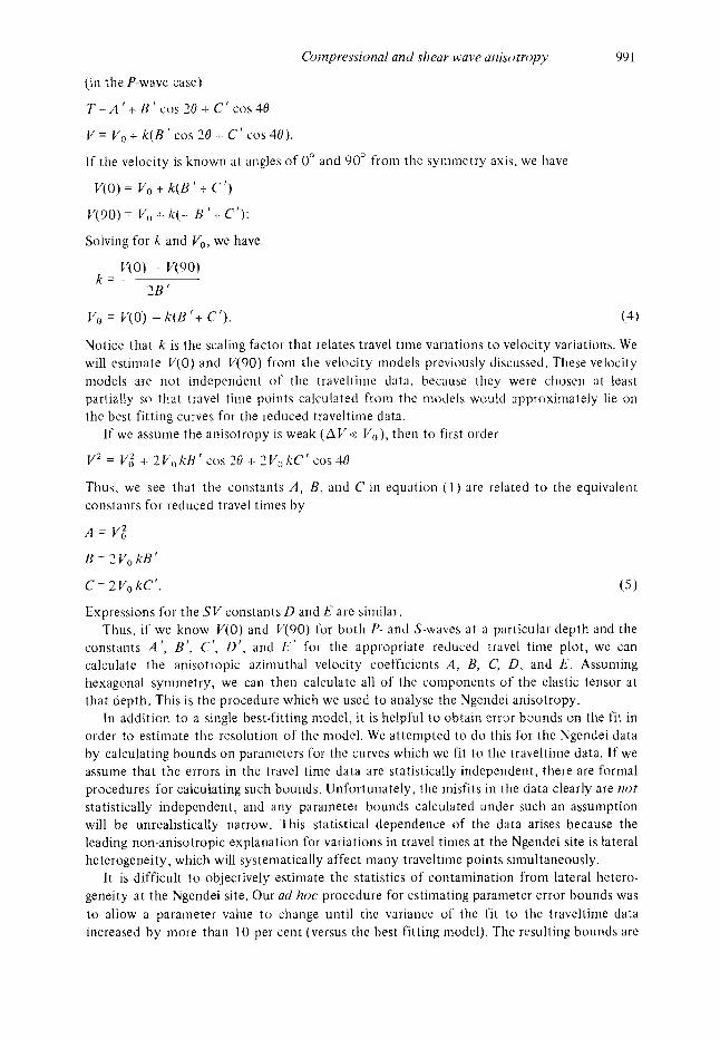
Obtaining elastic constants from travel time data

In general, it is impossible t o completely recover the elastic constants of a medium from velocity measurements within a single plane. However, such recovery is possible under certain simplifying assumptions which we believe are realistic for the Ngendei crustal and upper mantle anisotropy. Using relationships first derived by Backus (1965) and discussed extensively by Crampin ( 1 977) we can approximate the azimuthal velocity dependence of P and SVwaves in a general, weakly anisotropic medium with a known horizontal symmetry axis as

Vg = A i- B cos 28 t C c o s 48

V i v = D t E cos 28;

0 is the angle from the symmetry axis and A , B, C, D , and E a r e constants. These constants are related t o components of the anisotropic elastic tensor by

r l l l l = A + B + C

where is the anisotropic elastic tensor (normalized by density) and we have assumed that the symmetry axis has a ( 100) orientation and the vertical axis is (001 ).

We believe that the assumptions of weak anisotropy and a horimntal symmetry axis are appropriate for the Ngendei data. Azimuthal crustal velocity variations are about +2 per cent; upper mantle variations are about +3 per cent. Small velocity variations alone do not establish the accuracy of these equations (see Crampin 1982; Backus 1982) but they are suggestive of weak anisotropy. As a furthcr check, we calculated the parameter oE, a measure of the size of thc deviation of an elastic tensor from a n isotropic tensor (Backus

1 0 r

9 -

h 8 - W v1 v

v) 7 - ui d > 6 -

t- 5 - I

4l 3

P. M. Shearer and J. A . Orcutt

Line 4b (MSS)

9 -

h 8 - P) In v

In 7 - ‘D

> 6 - i- 5 -

*

I

4 -

3 -

1 I I I I I I

10 20 30 40 50 60 70 Range (km)

Line 5b (MSS)

I I 1 I a 1

10 20 30 40 50 60 70 80 Range (km)

Figure 14. (a ) Ihrchole seismometer (MSS) data for lines 4 b and Sb. Seismograms have been corrected for topography. reduced a1 4.65 kin c - ’ , and scaled for range and shot weight. (b) (opposite) S-wave synthetic seismograms for lines 4b and 5b.

10-

9 -

,--. 8 - e, m v

dl 7 - 0 .f

6 -

k- 5 - I

4 -

3-

Compressiorial and shear wave anisotropy

Line 4b (WKBJ Synthe t ics )

I I I I I I I

10 20 30 40 50 60 70

Line 5 b

1 Range (krn)

(W K BJ Synthet ics)

98Y

I I I 1 I I I I

10 20 30 40 50 60 70 80 Range (km)

Figure 14 - conrinued

1982), and found that U E < 0.2 for all models which we will consider in fitting both the Ngendei crustal and upper mantle anisotropy. Since the above approximations are valid for aE @ 1 , we consider the weak anisotropy assumption t o be appropriate for the Ngendei anisotropy. The additional assumption of a horizontal symmetry axis is difficult to justify purely from the observations, but is appropriate for any type of anisotropy based upon a single preferred orientation o f cracks or crystals,

33

990

Under these assumptions we can recover some but not ail of the components of r from aziniuthal velocity nieasurements oi‘ P and SV. If we further restrict the form of the aniso- tropy to hexagonal with syiniiietry axis ( I OO), then knowledge of A , B, C, L), and I:’ is sufficient t o obtain all components of r. As we will discuss later, such hexagonal niodels are appropriate for upper crustal anisotropy resulting from vertical aligned cracks and upper riiantle anisotropy resulting from preferred crystal alignment with a horizontal symmetry axis. For such a hexagonal material, we have the symmetry relationships (Musgrave 1970)

P. M. Sheilrrr arid J. A. Orcut[

T h e i-eni;iining I7 independent componei:ts of I’ are zero. From our Ngendei velocity model we can obtain approximate vaiues for A , B, C, D , and

I for the crustal and upper mantle anisotropy which the model predicts. Assuming hexagonal symmetry we can use the above relationships t o derive approximate values for the anisotropic elastic constants. Ilowever, there is a remaining ambiguity (discussed by Crosson & Christensen 1969) in that we must specify if the symnietry axis ( 1 00) represents the slow o r the fast velocity direction. Essentially this is equivalent to deciding if the vertical velocity in our hexagonal model corresponds to the fast or the slow horizontal velocity. We will decide between these two possibilities by examining the physical models which we believe are tilost appropriate to explain our observed anisotrctpy. The aligned crack models which seem appropriate tor the upper crustal anisotropy contain a slow hexagonal symmetry axis. In contrast, the aligned olivine models considered likely for the upper mantle contain a fast hexagonal symmetry axis.

Previous sections of this paper have concentrated on obtaining P- and S-wave velocity vei-sus depth sections for two orthogonal azimuths. ‘l‘hese profiles could be ~isetl to estimate the constants A , R, C, L ) , and I:‘ in the above equations. However. iii order to make estimates of C (the 48 P-wave term) and to constrain possible errors, it is helpful to examine reduced traveltime data versus azimuth. As a first order approximation, assume that velocity perturbations at a particular depth are linear functions of traveltime perturbations. We thus have

V = V , + A V = V, + k A T .

Now assume that traveltime perturbations AT are related to azimuthal anisotropy such that

Compressional and shear wave anisotropqi 99 1

(in the P-wave case)

T = A ' + B ' cob 70 + C ' cos40

v= V , + X ( B ' coS 28 + c' cos 40) .

If the velocity is known at angles of 0" and 90" fiotn the symmetry axis, we have

V(O)= V , + k ( B ' + C ' )

V(90) = v,, + X( B '+ C').

Solving for h and Vo, we have

V(0) V(O0)

V , = V(0) - k(B I + C'). (4)

Notice that k is the scaling factor that relates travel time variations t o velocity variations. We will estimate V ( 0 ) and V(90) from the velocity models previously discussed. These velocity models are not independent of the traveltime data, because they were chosen at least partially so that travel time points calculated from the models would approximately lie on the best fitting curves for the reduced traveltime data.

If we assume the anisotropy is weak ( A V e V o ) , then to first order

V z = V i + 2 V o k B ' cos 20 + 2 V g k C ' c'os 40

Thus, we see that the constants A , B, and C i n equation ( 1 ) are related to the equivalent constants for reduced travel times by

A = V,'

B = 2 V , kH'

C=?,V,kC'. (5 1 Expressions for the SV constants D and E are similar.

Thus, if we know V ( 0 ) and V(90) for both P- and S-waves at a particular depth and the constants A ' , B ' , C', D ' , and k' for the appropriate reduced travel time plot, we can calculate the anisotropic azimuthal velocity coefficients A , B, C, D , and L'. Assuming hexagonal symmetry, we can then calculate all of the components of the elastic tensor a t that depth. This is the procedure which we used t o analyse the Ngendei anisotropy.

In addition t o a single best-fitting model, it is helpful t o obtain error bounds on the fit in order to estimate the resolution of the model. We attempted to d o this for the Ngendei data by calculating bounds on parameters for the curves which we fit to the traveltime data. If we assume that the errors in the travel time data are statistically independent, there are formal procedures for calculating such bounds. Unfortunately, the misfits in the data clearly are not statistically independent, and any parameter bounds calculated under such an assumption will be unrealistically narrow. This statistical dependence of the data arises because the leading non-anisotropic explanation for variations in travel times at the Ngendei site is lateral heterogeneity, which will systematically affect many traveltime points simultaneously.

It is difficult t o objectively estimate the statistics of contamination from lateral hetero- geneity a t the Ngendei site. Our ad hoc procedure for estimating parameter error bounds was to allow a parameter value t o change until the variance of the fit t o the traveltime data increased by more than 10 per cent (versus the best fitting model). The resulting bounds are

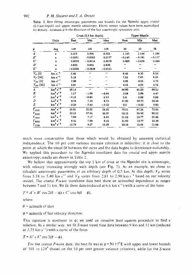
992 P. M. Slzearer and J. A . Orcutt Table 2. Best fitting anisotropic parameters and bounds for the Ngendei upper crustal (0.5 kni depth) and upper mantle anisotropy. Elastic tensor values have been normalized by density. Azimuth 0 is the direction of the fast anisotropic symmetry axis.

Crust (0.5 km depth) Upper Mantle

Units Best Min Max Best Min MaX

d deg 118 101 129 30 25 35

A' 9 0.315 0.308 0.323 1.165 1.144 1.186 B' 3 -0.0251 -0.0363 -0.0137 -0.149 -0.181 -0.117 C' S 0.0032 -0.0114 0.0178 0.000 -0.036 0.036 D' 0.622 0.604 0.636 - -

9

S

- - - - E' -0.0395 -0.0638 -0.0151

8.40 8.30 8.50 7.95 7.85 8.05 4.65 4.55 4.75

- - V p ( 0 ) kms-' 5.40 v, (90) km 11-1 5.18 - -

- - vs, (0) km sC1 2.90 VS, (90) km s-l 2.81 4.65 4.55 4.75 - -

66.83 65.26 68.53 - - A km's-' 28.13 B km' 8-' -1.17 -1.69 -0.64 3.68 2.89 4.47 c km's-' -0.15 -0.83 0.53 0.0 -0.89 0.89 D km' sCa 8.15 7.59 8.73 21.62 20.70 22.56 E km' (I-' -0.26 -0.42 -0.10 0.0 - 0.93 0.93

rllll km' 9-' 26.81 25.62 28.02 70.51 67.26 73.89

rzzzz km's-' 29.15 27.94 30.35 63.15 59.90 66.53

rlsls km' s-' 7.89 7.17 8.63 21.62 19.77 23.49 r1szs km' s-' 8.41 7.69 9.15 21.62 19.77 23.49 rll21 km's-' 12.79 9.27 16.26 23.59 15.61 31.66

much more conservative than those which would be obtained by assuming statistical independence. The 10 per cent variance increase criterion is subjective; it is close to the point at which the visual fit between the curve and the data begins to deteriorate noticeably. We applied this procedure to the Ngendei traveltime data for crustal and upper mantle anisotropy; results are shown in Table 2.

We believe that approximately the top 1 k m of crust a t the Ngendei site is anisotropic, with velocity increasing strongly with depth (see Fig. 7). As an example, we chose to calculate anisotropic parameters a t a n arbitrary depth of 0.5 kin. At this depth, V p varies f rom 5.18 to 5.40 kin s-' and Vs varies from 2.81 to 2.90 kin s-I based on our velocity model. The crustal P-wave traveltime data best show an azimuthal dependence at ranges between 7 and 11 kin. We fit these data (reduced at 6.6 km s-') with a curve of the form

T = A 'I- B' cos ~ ( 0 - 6) + cr cos 4(0 ~ 6), where

0 = azimuth of shot

4 = azimuth of fast velocity direction.

This equation is nonlinear in 4; we used an iterative least squares procedure to find a solution. In a similar way, we fit S-wave travel time data between 9 km and I 1 km (reduced at 3.75 kin s-') with a curve of the form

T = D'+ E' cos 2(0 - cp).

For the crustal P-wave data, the best fit was at 4 = N1 17"E with upper and lower bounds of 101 t o 129" (based on the 10 per cent greater variance criterion), while for the S-wave

Compressional and shear wave anisotrop,v 993

data the best fit was a t $J = 1 19" with bounds of 97" to 134". The close agreement between the azimuths of the fast P-wave direction and the fast S-wave direction ( 1 17" versus 119") suggests a symmetry axis in an anisotropic material. For consistency we used @ = 11 8" for subsequent analysis of both the P- and S-wave data. We took the intersection of the P- and S-wave bounds on @ to be the true bounds on @ ( l O l 0 to 129").

Using @ = 1 18", we calculated the best fitting values for A ', B : C', D' , and El. We then forced each parameter to higher and lower values (solving for tlie best fit for the remaining parameters) until the variance of the solution was 10 per cent more than the original variance. Table 2 contains the best fitting values with upper and lower bounds. Note that the limits on the parameters represent extremal bounds for one parameter at a t ime; in general, a curve using two or mvre of these bounds together would exceed the 10 per cent criterion for allowed increase in misfit variance.

Next, we used our values for V p and Vs at 0 and 90" (from the fast direction) and the relationships i n Equation (4) and (5) to calculate the velocity anisotropy coefficients A , B, C, D , and E . We switched the signs of B and E so that the horizontal symmetry axis would correspond to the slow direction, a relationship appropriate for the crack models which we will consider later. Bounds on U, C, ,and I:' were calculated from the equivalent bounds on B\ c', and E'. We assumed that A , related to the absolute h v a v e velocity, was precisely known. Clearly this is unrealistic at an exact depth of 0.5 kni, but since velocities are increasing rapidly with depth, i t is apparent that an appropriate value could be found close to the 0.5 km depth. The bounds shown on D in Table 2. were estimated subjectively, and represent the uncertainty in the absolute S-wave velocity relative t o the P-wave velocity (equivalent to uncertainty in tlie azitnuthally averaged Poisson's ratio), an uncertainty we assumed t o be kO.1 kin s-I.

Finally, using the relationships in (2) and (3), we calculated the best fitting values for the elastic constants for a hexagonally symmetric anisotropic material with a (slow) horizontal symmetry axis. We also calculated bounds on the elastic constants by using the appropriate extremal values of A , B, C, D, and E, but , because we used extremal values of more than one parameter at a time, these bounds are looser than the bounds on A , B, C, D , and E. In fact, they are so loose that they are of little practical use for comparison with physical models. These bounds could be tightened by directly searching for limits on the linear combinations of A , B, C, D , and E which are contained in (2) and (3). However, it is easier to simply calculate model values for A , B, C, D , and f? and compare these parameters to the data, rather than cornparing the elastic constants.

We used a similar procedure for analysing the Ngendei upper mantle anisotropy, but were limited by less complete data. Since S, was observed at only two azimuths, we were unable t o tit a curve t o the S-wave upper mantle data. Because of the limited azimuthal coverage of the OBS P-wave traveltime data for the upper mantle (see fig. 19, Shearer & Orcutt 1985), we excluded 40 terms from the traveltime fit. In order to estimate C', the 40 traveltime coefficient, we examined other studies of P-wave upper mantle anisotropy in the Pacific which used much larger data sets (Raitt et al. 1969; Morris, Raitt & Shor 1969). These studies found that the 48 terms were small compared t o the 28 terms, with magnitudes generally less than 20 per cent of the 20 term magnitude. Thus, assuming that the Ngendei upper mantle anisotropy is similar to that observed elsewhere, we assigned a 'best' value of C' of zero, with lower and upper bounds defined by 20 per cent of the maximum value of

The best P-wave fit for 4, the fast direction, was N30"E, with lower and upper bounds of 25 and 35". Values and bounds for A ', B', and C'are shown in Table 2. I t is interesting to note that the calculated fast direction of the upper mantle anisotropy (N30'E) is very close

B I .

994

to 90' away from the fast direction in the upper crust (N118"E). From our two orthogonal velocity models we obtained values for Vp(0) and Vp(90.) of 8.4 and 7.95 km s-', respectively. and a single velocity o f 4.65 kin s-' for Vs(0) and ys(90). We then calculated best values for the velocity parameters A , B, C, D , and f (including bounds on 11 arid C?. I n order t o obtain tlie remaining bounds. we needed a measure ot' tlie uncertainty in our estimates of the upper mantle P- and ,3-wave velocities. Based on the synthetic seismogram modelling, we estimated this uncertainty in upper mantle velocities to be kO.1 km sC1, and we used this value t o infer bounds on A , L). and E. Notice that for the upper mantle we assumed that the horizontal symmetry axis corresponded to the fast direction. and thus it was not necessary to switch the signs o f H and /:'as we did for the crustal anisotropy. We would expect anisotropy of this type if the upper mantle anisotropy is caused by aligned olivine crystals.

P. M. Sheurer and J . A. Orciitt

Anisotropy from aligned cracks

Several candidate physical models might explain the anisotropy wliicli we observed a t tlie Ngendei site. In a previous paper (Shearer & Orcutt 1985), we discussed possible causes of the observed Ngendei crustal P-wave anisotropy and concluded that aligned cracks within the uppei- crust was the niost likely cause. We have liow refined O U T estimates of the depth arid extent o f the uppel- crustal anisotropy. and believe that aligned cracks within approximately tlie top 1 - 1.5 kin of crust are responsible for tlie observed P- and S-wave anisotropy. The presence of such aligned cracks is not unexpected since systems of oriented cracks have been directly observed on tlie surface of the oceanic crust (see for example Ballard & van Aiidel 1977; Luyendyk & Macdonald 1977; Ballard, van Andel di Molcomb 1981), and cracks have been hypothesized to explain other crustal marine anisotropy observations (Stephen 1981. 1985; White & Whitinarsli 1984). Furthermore since i t is widely believed that tlie sharp velocity gradients a t t h e top of the crust are a direct result of decreasing porosity in the crust (Spudich & Orcutt 1980b; Bratt & Purdy 1984), it s e e m likely that cracks could cause a directional velocity dependence as well.

Many theoretical studies of tlie effects of aligned cracks on elastic parameters have been done (Anderson, Minster & Cole 1974; Carbin & Knopoff 1973, 1975a, 197%; Crampin, McGonigle & Bamford 1980). For the purposes of this paper, the most useful treatment is presented by Hudson (1981, 1982), as explained and illustrated by Crampin (1984). The Hudson equations provide approximate expressions for the components of the anisotropic elastic tensor in the long wavelength limit for a weak distribution of parallel penny-shaped cracks, in terms of the Lame parameters of the host solid and the material within the cracks, the crack density and the crack aspect ratio. The crack density

Nu =--

U

where A' is the number of cracks of radius a in volume u , and the aspect ratio

c

U

u ' = -

where c is the crack thickness. The theory is valid for low crack densitics ( E d I ) and small aspect r a t i o s ( d c I ) .

The examples which Crampin discusses in his paper suggest a difference between dry and wet crack models in which dry crack models are defined by 70 P-wave velocity variations and wet crack models are defined by 40 variations. This presents a problem since the

Compressional and shear wave anisotrop,v 995

observed Ngendei P-wave crustal anisotropy is 26 dominant, but cracks near the top of old oceanic crust are almost certainly saturated. However, wet crack models need not be 40 dominant; their characteristics are a strong function of the aspect ratio d. At aspect ratios appropriate for very thin cracks (d < 0.001), such as those used in the Crampin paper, P-wave velocity variations are almost entirely 40, but a t larger aspect ratios appropriate for thicker cracks (d = 0.1 to 0.01), velocity variations are largely 20. At an aspect ratio of 0.005, 26 and 48 terms are approximately equal. This aspect ratio dependence explains the difference in the theoretical wet crack studies of Anderson er al. (1974), who found 28

P-wave 2 8 term ~ ~~

0

- = C a,

x n

m o o V

P-wave 48 term

- 0 001 0 01 0 1

Crack Aspect Ratio

I 0 0 1 0 01 0 1

Crack ASDeCt Ratio

0

w.

YI C m

1 V

V

I - n

m o o 1

1

I 0 1

Ngendei Bounds 7-

- 0 . 5

-0 03

I - 00 1 0 01 0 1

Crack Aspect Ratio

L - 0 0 0 1 0 0 1 0 1

Crack Aspect Ratio

Figure 15. Values of the velocity paramctcrs 8, the 20 /'-wave coefficient, C. the 40 /'-wave coefficient, and E , (tic 20 S-wave ioefi'icient, xrc contonred f o r different values o f the crack density F and crack aspect ra t io d in a theoretical model of parallel, penny-shaped cracks by Hudson (1982). The shaded regions indicate the appropridte bounds on R, C and F from the observed Npendei crustal anisotropy. The final shaded repion is thc intersection of these bounds.

996

P-wave velocity variations for fluid-filled cracks with aspect ratios of 0.01 to 0.80, with those of Garbin & Knopoff (1973) who found 48 velocity variations for infinitely thin cracks.

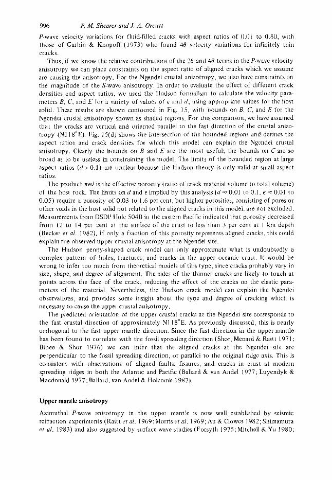
Thus, if we know the relative contributions of the 28 and 40 terms in the P-wave velocity anisotropy we can place constraints o n the aspect ratio of aligned cracks which we assume are causing the anisotropy. For the Ngendei crustal anisotropy, we also have constraints on the magnitude of the S-wave anisotropy. In order t o evaluate the effect of different crack densities and aspect ratios, we used the Hudson formalism to calculate the velocity para- meters B, C , and E for a variety of values of E and d , using appropriate values for the host solid. These results are shown contoured in Fig. 15 , with bounds on B, C, and E for the Ngendei crustal anisotropy shown as shaded regions. For t h s comparison, we have assumed that the cracks are vertical and oriented parallel to the fast direction of the crustal aniso- t ropy ( N I 18'E). Fig. 15(d) shows the intersection of the bounded regions 2nd defines the aspect ratios and crack densities for which this model can explain the Ngendei crustal anisotropy. Clearly the bounds on B and E are the most useful; the bounds on C are so broad as to be useless in constraining the model. The limits of the bounded region a t large aspect ratios ( d > 0.1) are unclear because the Hudson theory is only valid at small aspect ratios.

is the effective porosity (ratio of crack material volume to total volume) of the host rock. The limits on d and E implied by this analysis (d = 0.01 to 0.1, E = 0.01 t o 0.05) require a porosity of 0.03 t o 1.6 per cent, but higher porosities, consisting of pores or other voids in the host solid not related t o the aligned cracks in this model, are not excluded. Measurements from DSDP Hole 504B in the eastern Pacific indicated that porosity deci-eased from 12 to 1 4 per cent at the surface of the crust to less than 3 per cent at I km depth (Becker et 01. 1982). If only a fraction of this porosity represents aligned cracks, this could explain the observed upper crustal anisotropy at the Ngendei site.

The Hudson penny-shaped crack model can only approximate what is undoubtedly a complex pattern of holes, fractures, and cracks in the upper oceanic crust. It would be wrong to infer too much from theoretical models of this type, since cracks probably vary in size, shape, and degree of alignment. The sides of the thinner cracks are likely to touch a t points across the face of the crack? reducing the effect of the cracks on the elastic para- meters of the material. Nevertheless, the Hudson crack model can explain the Ngendei observations, and provides some insight about the type and degree of cracking which is necessary t o cause the upper crustal anisotropy .

The predicted orientation of the upper crustal cracks a t the Ngendei site corresponds t o the fast crustal direction of approximately N118"E. As previously discussed, this is nearly orthogonal t o the fast upper mantle direction. Since the fast direction in the upper mantle has been found t o correlate with the fossil spreading direction (Shor, Menard & Raitt 1971 ; Bibee & Shor 1976) we can infer that the aligned cracks a t the Ngendei site are perpendicular to the fossil spreading direction, o r parallel to the original ridge axis. This is consistent with observations of aligned faults, fissures, and cracks in crust a t modern spreading ridges in both the Atlantic and Pacific (Ballard & van Andel 1977; Luyendyk & Macdonald 1977 ; Ballard. van Andel & Holconib 1982).

P. M. Shearer and J. A. Orcutt

The product

Upper mantle anisotropy

Azimuthal P-wave anisotropy in the upper mantle is now well established by seismic refraction experiments (Raitt er al. 1969; Morris et al. 1969; Au & Clowes 1982; ShiInaniura r t al. 1983) and also suggested by surface wave studies (Forsyth 1975; Mitchell & Yu 1980;

Compressional and shear wuve anisotropy 997

Kawasaki & Kon'no 1984). The velocity anisotropy can b e described b y a cos 20 function of azimuth with the fast direction generally perpendicular to the local magnitude anomaly pattern and thus parallel to the original spreading direction. Anisotropy sitnilar in magnitude and orientation has been observed in ophiolite upper mantle material (Peselnick & Nicolas 1978; Christensen & Salisbury 1979; Christensen 8~ Smewing 1981; Christensen 1984) and is largely a result of preferred orientation of olivine crystals. Thus, the original observation and interpretation of upper mantle anisotropy by Hess ( 1 964) seems confirmed.

For these reasons, the observation of azimuthal upper mantle P-wave anisotropy at the Ngendei site is not surprising. I t seems likely that all oceanic upper mantle anisotropy is of similar origin, and thus the Ngendei anisotropy probably results from a preferred alignment of olivine crystals along a fossil spreading direction o f N30"E. Individual olivine crystals are orthorhombic and highly anisotropic with an a-axis P-wave velocity of 9.89 km s-', b-axis velocity of 7.73 kin s-', and c-axis velocity of 8.43 k m s- ' (Kumazawa & Anderson 1969). The ophiolite studies have shown that the a-axis tends to align parallel to the original spreading direction with the b- and c-axes confined to a vertical plane perpendicular to this direction. Within this plane, observations suggest that the h- and c-axes have little or no preferred orientation. The resulting anisotropy is approximately hexagonally symmetric with a horizontal symmetry axis corresponding to the fast P-wave direction. This is the justification for the assumptions which we made in solving for the elastic constants for the upper mantle.

Although the Ngendei S, arrivals were very weak. we believe that they do constrain the upper mantle SV velocity to be 4.65 * 0.1 km s-' a t two azimuths, approximately

A n i s o t r o p y of Oman H a r z b u r g i t e N

P-waves

8 . 2 t o 8 . 9 k m l s e c E

E SV-waves

4 . 7 to 4 . 8 km/sec

N

SH-waves

5 .0 k m l s e c

Figure 16. 1:qualarea projections of averaged velocities from samples of the Oman ophiolite (from Christensen & Smewing, 1981). Velocities are in km s-'. The cross in the V p diagram indicates the position of the normal to the sheeted dikes within the complex, the inferred direction of fossil spreading.

998

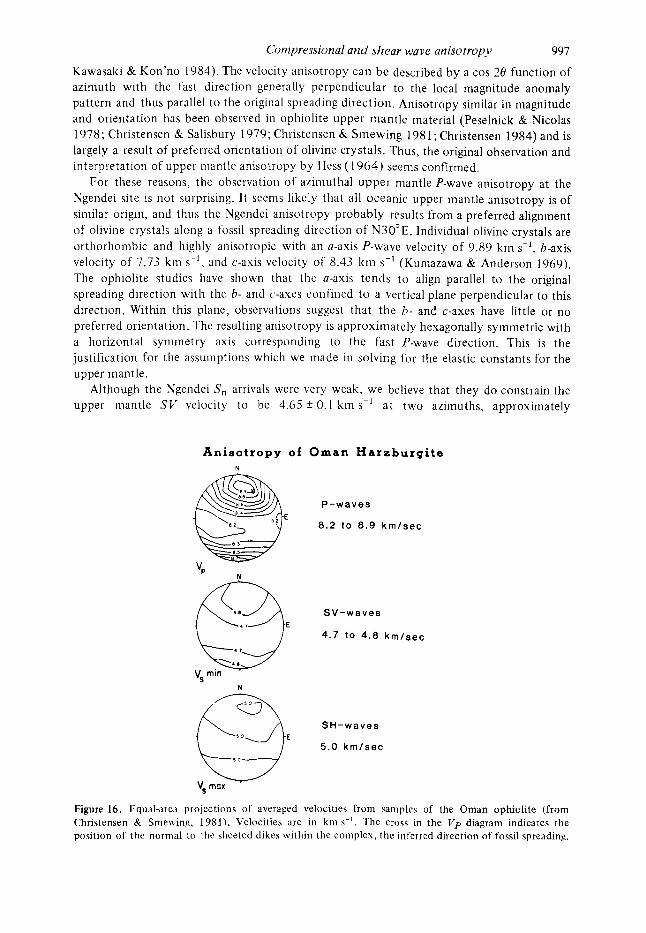
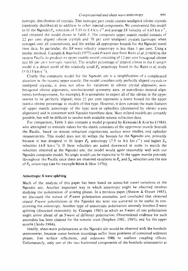
corresponding to the slow and fast P-wave directions. If we assulne that one SV velocity is high by 0.1 kin s-’ and the other low by 0.1 kin S - ’ ~ this still limits the upper mantle SV- wave anisotropy at the Ngendei site to be less than 52 per cent compared with observed P-wave anisotropy of *3 per cent. These results are similar t o refraction results of Clowes & Au (19821, who found upper mantle S-wave anisotropy of + 1 per cent and P-wave aniso- t ropy of * S per cent. The smaller SV-wave velocity differences compared to the P-wave differences are consistent with ophiolite studies. For example, Peselnick & Nicolas (1978) calculated velocity differences for a harzburgite sample (a t 5 kbar and 250°C) from the Antalya ophiolite in Turkey and found P-wave velocity differences of +5 per cent and corresponding SV velocity differences of k2.5 per cent. Fig. 16, reproduced from Christensen ti Smewing (1981), shows average velocities for samples from the Oman ophiolite. The slower shear wave velocity corresponds t o S V in an oceanic refraction experi- ment , and the faster shear wave velocity to SH. The approximately hexagonal nature of the anisotropy is clear, as well as the smaller directional variations of SV-waves compared to P-w av e s .

These properties can also be seen directly in the anisotropy of olivine crystals. We calculated the elastic constants for an aggregate of olivine crystals with fixed a-axis orientation and random h- and c-axes orientations within a vertical plane, by averaging the elastic tensor for olivine over the possible orientations. This is equivalent to the Voight averaging scheme for determining aggregate elastic properties from single crystal data (see Crosson & Lin (1 97 1) for a discussion). We used values for elastic constants of olivine from Kurnazawa & Anderson (1 969), uncorrected for pressure and temperature. Table 3 contains values for the resulting hexagonally symmetric elastic tensor, and, for comparison, the Ngendei upper mantle results. The hexagonal olivine niodel has azimuthal P-wave velocity anisotropy of *I0 per cent and SV-wave anisotropy of 23.5 per cent. We also show the approximate velocity coefficients A , B, C, D, and E , but these are not very accurate for off- axis velocities because of the large anisotropy of the hexagonal olivine model (aE = 0.62).

A more realistic upper mantle model will contain other crystals in addition to the aligned olivine crystals. Using the Voight averaging scheme, we created a composite upper mantle model which consists of the weighted average of aligned olivine crystals and a purely

P. M . Shearer a n d J. A. Orcutt

Table 3. Anisotropic parameters for the Ngendei upper mantle data compared with an olivine based model and a model proposed b y Kawasaki & Kon’no (1984). Units are as in Table 2.

Ngendei Model Crystal Aggregate Model Kawasaki

Best Min Max Olivine Host Both & Kon’no

70.51 67.26 73.89 97.77 62.82 70.51 73.94 63.15 59.90 66.53 64.48 62.82 63.18 62.12 21.62 19.77 23.49 23.72 21.50 21.99 22.73 21.62 19.77 23.49 20.39 21.50 21.26 20.91 23.59 15.61 31.66 20.83 19.82 20.04 21.82

66.83 65.26 68.53 77.91 62.82 66.14 67.84 3.68 2.89 4.47 16.65 0.0 3.66 5.91 0.00 -0.89 0.89 3.21 0.0 0.71 0.19

21.62 20.70 22.56 22.05 21.50 21.62 21.82 0.0 -0.93 0.93 1.67 0.0 0.37 0.91

8.40 8.30 8.50 9.89 7.93 8.40 8.60 7.95 7.85 8.05 8.03 7.93 7.95 7.88

vs, (0) 4.65 4.55 4.75 4.87 4.64 4.69 4.77

v.q, (90) 4.65 4.55 4.75 4.52 4.64 4.61 4.57

GI mpressioizal arid shear wave aiziso t r0p.v 999

isotropic distribution of crystals. This isotropic part could contain unaligned olivine crystals (randomly distributed) in addition to other mineral components. We constrained this model to fit the Ngendei P, velocities of 7.95 t o 8.4 kin s-' and average SVvelocity of 4.65 kin s-' , and obtained the model shown i n Table 3. The coniposite upper mantle model consists of 22 per cent aligned olivine crystals and 78 per cent unaligned crystals (isotropic when averaged over all orientations), and fits within all appropriate bounds for the Ngendei travel time data. In particular, the SV-wave velocity anisotropy is less than I per cent. Using a similar method. Crampin & Baniford (1977) used P-wave data froin Raitt er a / . ( 1 969) in the eastern Pacific to produce an upper mantle model consisting of I1 per cent hexagonal olivine and 88 per cent isotropic matet-id. The snialler percentage of aligned olivine in the Cranipin model is a direct result of the relatively small P, anisotropy found in the Raitt ef al. study (+ 0.1 5 kin s- ' ) .

Clearly this composite model for the Ngendei site is a simplification of a complicated situation i n the oceanic upper mantle. The model considers only perfectly aligned crystals o r unaligned crystals; it does not allow for variations in olivine crystal alignment, non- hexagonal olivine alignments, non-horizontal symmetry axes, or non-olivine mineral align- ments (orthopyroxene, for example). I t is unrealistic to expect all of the olivine in the upper mantle t o be perfectly aligned; thus 22 per cent represents a lower bound for the upper mantle olivine percentage in models of this type. However, it does contain the main features of upper mantle anisotropy of the type seen in ophiolites (dominated by olivine a-axis alignment) and is consistent with Ngendei traveltime data. More refined models are certainly possible, but will be difficult t o resolve with available seismic refraction data.

For comparison, Table 3 also contains a model proposed by Kawasaki & Kon'no (1984), who attempted t o estimate values for the elastic constants of the uppermost mantle beneath the Pacific, based on seismic refraction experiments, surface wave studies, and ophiolite measurements. This niodel does not fit within the bounds for the Ngendei site, primarily because it was designed to fit larger P, anisotropy (7.9 to 8.6 km s-') and higher S, velocities (4.8 km s-'). If these velocities are scaled downward in order t o match the velocities observed at the Ngendei site, the model would agree reasonably well with our Ngendei composite model. No single model can be expected to fit the upper mantle precisely throughout the Pacific since there are observed variations in P, and S , velocities and the size of P, anisotropy (see for example Bibee & Shor 1976).

Anisotropic S-wave splitting

Much of the analysis of this paper has been based on azimuthal travel variations at the Ngendei site. Another important way in which anisotropy might be observed involves studying the polarization of arriving phases. In a previous paper (Shearer & Orcutt 1985). we discussed the nature of P-wave polarization anomalies, and concluded that observed crustal P-wave polarizations at the Ngendei site were too scattered to be useful in con- straining the anisotropy. Another type of anisotropic polarization anomaly involves 5'-wave splitting (discussed extensively by Crampin 1985) in which an S-wave of one polarization might arrive ahead of an S-wave of different polarization. Observational evidence for such anomalies has been claimed for the oceanic crust (Stephen 1981, 1985), and for the upper mantle (Ando 1984).

Ideally, shear-wave polarizations at the Ngendei site would be observed with the borehole seismometer, because ocean bottom recordings suffer from problems of converted sediment phases, free surface reflections, and unknown OBS t o seafloor coupling effects. Unfortunately, only one of the two horizontal components of the borehole seismometer a t

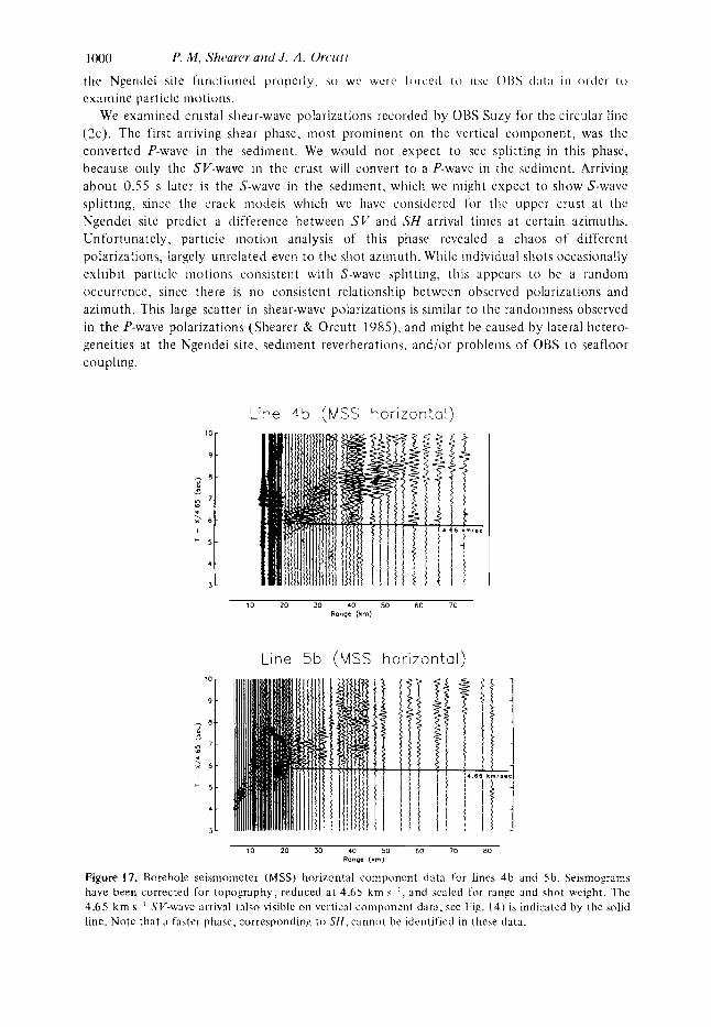
1000

the Ngendei site f u n c t i o n 4 properly. so we wcic l'orc,ecl to IISC OI%S d a t a 111 oitiet to examine particle inotioiis.

We examined crustal shear-wave polarizations recorded by OBS S u ~ y for tlie circular line (2c). The first arriving shear phase, most prominent on tlie vertical component, was the converted P-wave in the sediment. We would not expect to see splitting in this phase, because only the SV-wave in tlie crust will convert to a P-wave in the sediment. Arriving about 0.55 s later is the S-wave i n the sediment. which we might expect t o show S-wave splitting, since the crack inodels which we liave considered for the upper crust at the Ngendei site predict a difference between S V and SH arrival times at certain azitnuths. Unfortunately, particle motion analysis of this phase revealed a chaos of different polarizations. largely unrelated even to the shot azimuth. While individual shots occasionally exhibit particle motions consistent witli S-wave aplitting, this appears t o be a random occurrence, since there is n o consistent relationship between observed polarizations and azimuth. This large scatter in shear-wave polarizations is similar to the randomness observed in the P-wave polarizations (Shearer & Orcutt 1985). and might be caused by lateral hetero- geneities at the Ngendei site, sediment reverberations, and/or problems of OBS to seafloor coupling.

P. hi. Shcarw arid J . A . 0rC.riti

I0

9 -

- 8 -

.n 7 -

., t

3 6 -

* 5 -

I

.- ,

Line 4 b (MSS h o r i z o n t a l )

-

, .. ... ,.......... ..

10 20 30 40 50 60 70 Range (km)

Line 5 b (MSS h o r i z o n t a l )

10 20 30 40 50 60 70 80 Ronga (hm)

Figure 17. Borehole seismometer (MSS) horizontal component data for lines 4b and 5b. Seismograms have been corrected f o r topography, reduced a t 4.65 km K ' , and scaled for range and shot weight. The 4.65 krn R-' SV-wave arrival (a lso visible on vertical component data. see I3g. 1 4 ) is indicatcd by the solid line. Note that a faster phasc, corresponding to SI I , cannot be identitied in these data.

Compressional and shear wave anisotrop?, 1001

Similarly, upper mantle models predict that SH waves should arrive ahead of SV-waves at certain azimuths. OBS data at tnantle ranges are too noisy to even identify the S, phase, so the borehole seismometer (MSS) data provided our only hope of seeing upper mantle shear- wave splitting. As previously discussed, we identified a weak upper mantle SV phase on the vertical component of the MSS, and calculated its velocity at approximately 4.65 kni s-l for both line 4 b and line Sb. We examined the single horizontal component of the MSS (unknown orientation) but were unable to identify a phase which might correspond to SH (see Fig. 17). We do not consider this evidence against upper mantle anisotrupy. because a weak SH phase could easily be lost in the noise. In addition, significant SH-wave energy is not always efficiently generated in marine refraction experiments, because it requires scattering of seismic energy out of tlie sagital plane by lateral heterogeneities and/or off-axis aiiisotropy.

Conclusions

The 1983 Ngendei expedition to the south Pacific detected anisotropy both within the upper crust and the uppermost mantle. Shear-wave travel times indicate azimuthal 5'-wave anisotropy in the crust, which, together with tlie P-wave anisotropy previously observed, is sufficient to calculate anisotropic elastic constants (under a n assumption of hexagonal symmetry). The upper crustal anisotropy is probably caused by aligned cracks parallel t o tlie original ridge axis at the Ngendei site. Constraints on anisotropic parameters in the upper crust are consjstetit with a penny-shaped crack model involving crack aspect ratios of 0.0 I t o 0.1.

Despite Ngendei P, anistropy of 7.95 to 8.4 kni s-', S , velocities are close t o constant at 4.65 kni s-'. The observed upper mantle anisotropy agrees with previous seismic experiments and ophiolite studies, and suggests that tlie fossil spreading direction at tlie Ngendei site was N30"E. Calculated expressions for tlie anisotropic elastic constants are consistent with a simple model of thc upper mantle consisting of '2'2 per cent aligned olivine crystals. The character of the velocity profiles derived from synthetic seismogram inodelling is in general agreement with other refraction studies.

Acknowledgments

This research was supported by DAKPA contract AFOSR-84-0043. We thank the scientists and crew on the R/V Melville and D/V Glotnar Challenger for making the Ngendei experiment a success. Steven Bratt provided a helpful review of this paper.

References

Adair, K. G., Orcutt, J . A . & Jordan, 'T. ti . , 1986. Preliminary analysis of ocean bottom and sub-bottom microseismic ambient noise during the Ngendei Experiment, Initial Rep. Deep Sea Drill Proj. , Leg 9 1, in press.

Anderson, I). L . , Minster, 13. 8: Cole. I) . , 1974. l h e effect of oriented cracks on seismic velocities, J . ~eophys. Res., 79, 401 1-4015.

Ando, M . , 1984. ScS polarization anisotropy around the Pacific Ocean, J. phys. EQrIh, 32, 179-1 95. Au, C. Y. D. & Clowes, R . M., 1982. Crustal structure from an ocean bottom seismometer survey in the

Hackus, G. I , . , 1965. Possible forms of seismic anisotropy of the uppermost mantle under oceans, J.

Backus, (;. I < . , 1982 Keply: limits of validity of first-order perturbation theory for quasi-P-velocity in

Nootka fault zone off western Canada, Geophys. J. R . astr. Soc., 68, 27-47.

,q~>pkys. Res., 70, 3429 --343 9.

weakly anisotropic media, J. gcophj>.s. Kes., 87, 4641 --4644.

1002

Hallard, R . I). & van 4nde1, T. I I . , 1977. Morphology and tectonics of the inner rift valley a t lat 36"50'N o n the Mid-Atlantic Ridge, Bull. geol. Soc. A m . , 88. 507--530.

I3allard. K. I)., van Andel. '1'. I I . & tlolcomb, R. T., 1982. The (;alapagos Rift a t 86"W: variations in volcanism, structure. and hydrothermal activity along a 30-kilometer segment ot the rift valley. J. Kcoplij's. Kcs.. 87. 1 149 . 1 16 1 .

Beckcr, K.. von Herzcn. K. I)., I'ranci\, I. J . (;., Anderson, R . N., tlonnorez, J . . Adamson, A . ('., Alt, J . C., l.mmerniann, R., Kempton, 1'. I)., Kinoshita, H., Laverne, C.. hlottl. hl. J . & N w r n a r k , R. L., 1982. Irr sitir electrical resistivity and bulk porosity of the oceanic crust Costa Rica Rift, :'Vature.

Hibee, L. I). & Shor. C;. G.. 1976. Coinpressional wave anisotrop) in t he crust and upper mantlc.

Hratt, S. R. & I'urdy. G. hl.. 1984. Structure and variability of oceanic crubt o n the flanks o f the Last

Chapman. C. H., 1978. .A new method for computing synthetic seismograms. (;eophjx. J. R. astr. Soc..

( 'hapman, (.. 11 . & Orcutt, I . j\.. 1985. The computation o f l>ody-\t:ive synthetic seismogr:irris in laterally

('liristcnsen. N. I . & Salisbury, 11. II., 1975. Structure and constitution o f the lower oceanic crust, Kci..

Christensen. N. I . & Smewing, J . D., 1981. Geology and seismic structure of the northern section of the

Christensen, N . I . , 1984. 'fhe magnitude, symmetry and origin o f upper mantle anisotropy based o n

('lowe.;, I<. hl. & Au, I). . 1982. [ti-sitrr evidence for :I low dcgrcr o f S-wave anisotropy in t h e oceanic

( 'rampin, S., 1977. A review of the effects uf anisotropic layering on the propapt ion of seismic waves,

('rampin. S. , 1982. ( 'oniments on 'possible forms of anisotropy of the uppermost mantle under oceans' by

( 'rampin, S., 19x4. I ffcctivc anisotropic elastic constants tor \F;IVC propagation through cracked solids,

P. M . Shearer and J. A. Orc*utt

300,594-598.

(;cop/i.i,s. Krs . I . c t r . . 3. 6 3 9 - 642.

Pacific Rise betifeen 11" and 13"N,J.gcop/iys. H e x , 8 9 , 6 1 1 1 -6125.

5 4 . 4 8 1 - ~ 5 1 8.

honiopcncous media, Hci!. (;cop/!j,s. Spac~, P/I>~.Y.. 23. 105 163.

Geophys. Space P/iys., 13, 57 -86.

Oman Ophiolite. J. gcopli.v.s. Res., 86, 2545--2555.

taliric analyses of ultranialic tcctonites, (;eophj2s. J. R . astr. Soc.. 76. X9

upper mantle, (;eophj*s. Res. lxt t . , 9 , 13--16.

( ;eopl i~s . J. R. astr. Soc., 49, 9-27.

(korge 1 , . Ihckus. .I. ~ e o p h j ~ s . R c s . , 8 7 , 4636- 4640.

(;eop/rys. J. R. astr. Soc.. 76. 135-145.

1 1 1 .

1985. I,,valuation of anisotropy by shear-wave splitting, (;eop%,~sics. 50. 142-152. Crampin, S. & Baniford. 11.. 1977. Inversion ofP-\tave velocity anisotropy, (;cop/iys. J. R. astr. Soc.. 4 9 ,

Crampin, S. , McConigle, R . & Bnniford. D., 1980. Estimating crark parameters from observations of

C'riisson, K. S. & Chnstcnscn. N. I., 1969. Transverse isotropy o r thc upper mantle in the vicinity of

Crosson. R. S. & Lin, J . W.. 1971. Voight and Keuss prediction of anisotropic elasticity of Dunite, J.

l ,orsyth, L). W . , 1975. 'Ihe early structural evolution and anisotropy o f the oceanic upper mantle,

I~'uchs, K . & hlilller. G., 1971. Computation of synthetic seismograms with the reflectivity method and

Garbin, H . D. & Knopoff, L. . 1973. The compressional modulus of a material permeated by a random

(;arbin. I I . I). & Knopoff, L., 19752. T h o shear modulus of'a material pcrmeatcd b y ii rnndoni distribution

Garbin. I I . D. & Knopoff. L., I975b. I h s t i c moduli o f 1 mediuni with liquid filled cracks, Q. uppi.

Carmany. J., 1981. Anisotropic gradients in the upper mantle, Geophys. Rcs. Let t . , 8. 955L957. Hart. K . S. & Press, I , . , 1973. S, velocities and the composition of the Lithosphere in the regionalized

lless, 11. t l . . 1964. Seismic anisotropy o f the uppermost mantle under oceans, Nurture, 203. 6 2 9 - - 6 3 l . Hudson, J . A,. 1981. Wave speeds and attenuation of elastic \vaves in material containing cracks, ( ;eop/r j~s .

Hudson. J. A, , 1982. Overall properties o f a crack solid. Math. Proc. Currth. Phil . Soc.. 88. 371 -384. Kawasaki. 1. & Kon'no. I . .. 1984. Azimuthal anisotropy of surface waves and the possible type o f thr

123--132.

P-wave velocity anisotropy, Ccoplivsics. 45, 345 --360.

Pacific fracture zones. Bull. seismol. Soc. An7., 5 9 , 59-72.

geophys. Rcs., 76. 570-578.

Geopltys. J. R. astr. Soc., 4 3 , 103--162.

comparison with observations. Geophys. J. K. astr. Soc.. 23. 41 7V433.

distribution of circular cracks, Q. oppl. Matlr.. 30. 453 -464.

of circular cracks, Q. oppf. rriotli., 33, 296 - 300.

Marl!., 33, 301 --303.

At1antic.J. geopliys. Hcs., 78, 407L411.

J. K.as t r . Soc., 6 4 , 133-150.

Corriprcssiotial and shear wave aiiisotrop.v 1003

seismic anisotropy due to preferred orientation of olivine in the uppermost mantle beneath the Pacific Ocean, J. P11j.s. Earfh. 32. 22Y -244.

Kim, I . I . , Smith, I). K., Mcnard, 1 1 . it.. Orcuti, J . ,\. & Jordan, 1. 1 1 . . 1986. Seismic reflection site survey: ('orrelation with physical properties, Leg 91. Deep Sea I)rilling Project, lnitial Rep., I k e p Sea Drill k o j . , 1 . q Y I ~ in prcu.

Kumazawa, M . 8: Anderson, I). L . , 1969. Elastic moduli. pressure derivatives, and temperature derivatives of singlei-rystal olivine and vinglecrystal fosterite,J. geoeophys. Res., 74, 5961 -5972.

Luyendyk, B. P. & Macdonald. K . C , . 1977. Physiography and structure of the inner floor of the I'AMOUS rift valley: observations with a deep-toived instrument packape. Hull. geol. Soc. . , I i f i . , 88. 648 663.

hlitchell, 13, J . & 'I'u, (;.-K., I 980. Surface \ \ ; IVC disper\ioti. rcgionaliied vclocily models. and anisotrop) of the Pacific crust and upper mantle, G e o p l i ~ ~ r . J. K . asrr. Soc., 63. 497-5 14.

Slolnar, P. Br Oliver, J . , 1969. Lateral variations o f attenuation in the upper mantle and discontinuities in the lithosphere. J. geopliyx. Rc~s.. 74. 1648 ~ 2682.

Vlorris, (;. H.. Raitt, R. h'. Br Shor. (;. (;., 1969. Velocity anisotropy and delay-time maps of the mantle near Ilawaii,J. , i !eopIij~.s. Kcxs., 74. 4300 ~ ~ 4 3 1 6 .

hlusgrave, hl . J . I ) . , 1970. C Pesclnick, L. 8 Nicolas, ,4., 1978. Seismic anisotropy in an uphiolite peridotite: application to oceanic

upper mantle, J. geopliys. Rcs., 8 3 , 1227 - 1235. Raitt, R. W., Shor, G. G., francis, 1. J . G. 8 klorris, G. B., 1969. Animtropy of the Pacific upper mantle,

J. Xeopliys. Kes. , 74, 3095 -3 109. Sereno, '1'. J. & Orcutt, 1. ,\., 1985. I he synthesis of realistic oceanic \\avc traii1s.J. ~ m p l r j ~ s . R r x , 90,

1 2 7 5 5 12176. Shearer, P. & Orcutt, J., 1985. Anisvtrupy in the oceanic lithosphere - theory and observations fioiii the

Ngendei seismic rct'raction experiment in the south\vest Pacific, Geoplrys. 1. R. m f r . Soc., 80, 493 -526.

Shearer, P. Jl., Orcutt, J . A , , Jordan, T. ll., \Vldtmarsh, R. B., Kim, I. I . . Adair, R. (;. & Burnett, hl. S. , 1986a. The Ngcndei scisinic refraction expcrirnent at I)SI)I' llole 59513 ocean h t t o m scismo- iiicter data and cvidcncc ]'or crustal and upper mantle anisotropy, lnitial Rcp., I )CV/J Sca Drill. Proj. , Leg 91 , in press.

Shearer, P. M., Adair. R. G., Orcutt, J . A. & Jordan, I. l i . , 1986b. Simultaneous borehole and ocean bottom seismometer recordings of earthquakes and explosions - results from the 1983 Ngendei 1,xperiment at DSDP Hole 59513, hzitial Rep. Deep Sea Ilrill. fro]., Leg Y Z , in press.

Shimamura, ti., Asada, T. & Kumazawa, M . , 1977. High shear wave velocity layer in the upper mantle of the western Pacific, .Vatwe, 269, 6 8 0 -682.

Shiniamura, [I., Asada, T., Suychiro, K., Yamada, 'I. & Inatani, l i . , 1983. Lonpshot experiments to study velocity anisotropy in the oceanic lithosphere of the northwestern Pacific, PItys. Eartli plarief. h r . , 31,348-362.

Shor, G. G., Mennrd, H. W. & Raitt, K. W., 1971. Structure of the Pacific basin, The Sea, 4, (I]) , pp. 3-27, John Wiley & Sons.

Spudich, P. & Orcutt, J . , 1 980a. Petrology and porosity of an oceanic crustal site: results from wave form modelling of seismic refraction data, J. gcwpliys. H e x , 85, 1409-1433.

Spudich, P. Br Orcutt, J., 1980b. A new look at the seismic velocity structure of the oceanic crust, Rer?. GeopIiys. Space Pliys., 18,627-645.

Stephen, K. A,, 1981. Seismic anisotropy observed in upper oceanic crust, Geoph.ys. Res. Lett., 8, 865 ~ - 8 6 8 .

Stephen, K. A., 19x5. Seismic anisotropy in the upper oceanic crust, J. geeophys. Kes., 90, I 1 383-1 1396.

Walker, D. A . 8 Sutton, G. ti., 1971. Oceanic mantle phases recorded on hydrophones in the north- western Pacific a t distances between 9" and 40", Bull. seismol. SOC. Am., 61, 65-78.

Walker, D. A , , 1977. Iligh-frequency Pn and Sn phases recorded in the western Pacific, J. geophys. Res., 82,3350--3360.

White, R. S. & Whitmarsh, K. B., 1984. An investigation of seismic anisotropy due t o cracks in the upper oceanic crust at 45" N , Mid-Atlantic Ridge, (;eOphyS. J . R . ostr. Soc.. 79 ,439-467.

Whitmarsh, R. B., Orcutt, 1. A,, Jordan, T. li., Adair, R. G. & Shearer, P. M., 1986. Velocity bounds on the seismic structure of late Jurassic crust and upper mantle in the southwest Pacific basin from downhole observations at Deep Sea Drilling Project Hole 595B, Initial Rep. Deep Sea Drill. froj., LeR 91, in press.

t ~ l ..lc,otrsrics, tloldcn-l)ay.